Dynamic Performance Optimization of Sensorless PMSM System with Low Switching Frequency Based on Improved Deadbeat Control PLL

Abstract

The dynamic performance of sensorless PMSM control systems at low switching frequency is suboptimal due to issues such as position estimation error with proportional-intregral (PI)-based phase-locked loops (PLLs) and the inaccuracy of the system model. To solve this problem, this article first proposes an improved PLL based on a deadbeat controller with a damping factor (DDCPLL). It rapidly converges the estimated rotor position to the actual position during speed transients while ensuring the smoothness of the estimated speed. This approach reduces the number of undetermined coefficients from two in traditional methods to one, simplifying the structure and facilitating implementation. Additionally, to address the current cross-coupling issues in traditional current control strategies at low switching frequencies, a novel controller was directly designed based on the discrete-domain model of the PMSM. Then, by integrating the proposed DDCPLL, a discrete-domain model of the entire positionless control system was established. The parameters of the speed controller are optimized to further enhance the system’s dynamic response performance. Furthermore, the robustness of the system under speed estimation errors and motor parameter variations is analyzed. The results demonstrate that the proposed control system maintains good robustness despite the presence of speed estimation errors and parameter mismatches. The effectiveness and feasibility of the proposed PLL and control strategy are demonstrated by detailed results.

1. Introduction

PMSMs offer advantages such as high torque density, rapid dynamic performance, and exceptional reliability, making them widely adopted in industrial production, aerospace, and home appliance sectors. The most prevalent PMSM control strategy currently is dual-loop vector control, whose implementation hinges on accurately acquiring rotor position information. Traditional position detection methods involve installing position sensors on the motor shaft. However, the presence of position sensors not only increases the size and manufacturing cost of the motor drive system but also reduces its reliability. Therefore, the position sensorless control strategies hold significant theoretical and practical value and have become one of the primary research directions in the field of electric power transmission [1].

Sensorless control methods for PMSMs fall into two categories. One is the high-frequency injection method, suitable for the zero-to-low speed range, which primarily includes high-frequency rotational sinusoidal voltage injection (HF-RSVI), high-frequency pulse sinusoidal voltage injection (HF-PSVI), and high-frequency square wave voltage injection (HF-SWVI). Another type is the observer method suitable for medium-to-high speed ranges, primarily including flux linkage estimation, sliding mode observers, and extended Kalman filter algorithms. The common feature of the above methods is acquiring signals containing actual position information, then processing these signals to obtain estimated rotor position. The inverse tangent function can be used to calculate the rotor position angle, followed by differentiation to compute rotational speed. However, differentiation introduces noise and may even cause computational divergence. Therefore, a PLL is typically employed to replace the inverse tangent function [2]. There are various kinds of PLL so far, such as the synchronous reference frame type [3], the speed tracking type [4], and the heterodyne method [5]. However, conventional PLLs adopt a PI controller as the loop filter, constituting a second-order system. When the speed is a ramp signal, they cannot achieve accurate tracking of the actual position, resulting in limited dynamic performance of the overall system [6]. The finite-control-set phase-locked loop (FPSPLL) was proposed, which eliminates the need for tuning controller parameters and addresses the issue of rotor position estimation error during speed variations. Numerous studies have focused on reducing the number of iterations and improving convergence accuracy. Although the latest research has significantly lowered the computational cost, the position error theoretically does not reach zero [7,8,9]. Moreover, at low switching frequencies, the available sampling points are limited, which restricts the achievable accuracy and may lead to local convergence issues Based on adaptive algorithms, the adaptive phase-locked loop (APLL) optimizes dynamic performance by adjusting its bandwidth in real time. The core idea is to use a narrow bandwidth at low speeds to suppress noise and adaptively increase the bandwidth during acceleration to reduce position estimation errors. Due to its parametric flexibility, it has become a popular research topic. However, it is worth noting that APLL is still essentially a PI-type PLL; its transfer function structure remains unchanged, with only the parameters being adjusted in real time. This implies that under ramp speed variations, the error can only be reduced by increasing the bandwidth, but cannot be fundamentally eliminated [10]. An estimation compensation strategy for PLL was proposed in [11], which reduces the position tracking error during acceleration and deceleration by detecting the q-axis current differential. However, the introduction of the differential term degrades the anti-interference capability of the PLL. A feedforward PLL was presented in [12] to mitigate the rotor position estimation error under acceleration/deceleration conditions. Nevertheless, this method relies on the permanent magnet flux linkage parameter of the PMSM. A dual-PLL (DPLL) structure was introduced in [13,14]. It can theoretically achieve zero position error under a linearly increasing speed. However, as a fourth-order cascaded system, it exhibits complex dynamics and reduced stability margins compared to second-order systems. The dual-loop structure trades negative gain margin for performance, introducing stability risks. Thus, even with theoretical zero error, its practical dynamic performance may not surpass that of lower-order systems.

Additionally, in the high-power systems, operation at low switching frequencies is typically employed to effectively reduce switching losses and prolong the service life of power devices. However, the position sensorless control at low switching frequencies faces several challenges. First, as the switching frequency decreases, the current sampling period and the control period of the current loop increase, leading to large current loop delay and exacerbated dq-axis coupling. This consequently reduces the system stability margin [15]. Furthermore, the tuning of controller parameters and the design of observers are commonly conducted in the continuous-time domain, followed by discretization [16]. However, the discretization errors introduced during this process can adversely affect both the controller and the observer performance.

To address current decoupling issues, a two-degree-of-freedom discrete-time decoupled current control scheme with high parameter robustness was proposed in [17], retaining the parameter insensitivity of internal model control while enhancing control bandwidth and disturbance rejection. A complex vector PI current controller with deadbeat response was developed in [18], ensuring strong disturbance rejection and stability via a three-directional design considering dynamics, disturbance attenuation, and robustness. Furthermore, improved deadbeat predictive current control methods have been introduced—for example, a parameter adaptive incremental model-based DPCC eliminates parameter mismatch effects [19]. However, despite their respective advantages, inherent delays at low switching frequency and discretization errors continue to undermine the robustness of the control system. Several studies have focused on time delays in sampling and pulse-width modulation processes, analyzing bandwidth limitations and corresponding compensation methods [20,21,22,23]. In [22], a continuous-domain compensation approach applicable to carrier ratios below ten was proposed. Other researchers have concentrated on designing current controllers directly in the discrete domain. For instance, [24] analyzed and compared the effects of different discretization methods and developed corresponding compensation strategies accordingly.

In summary, it is highly worthwhile to investigate how to design a PLL that not only achieves zero rotor position estimation error during speed transients but also features a simple structure with easily tunable parameters. Furthermore, at low switching frequencies, the increased current loop delay and severe dq-axis current coupling remain challenging. Although some research has been conducted in this area, an effective method to eliminate the impact of discretization errors on the system is still lacking. Finally, current research remains largely confined to the current loop level; establishing an accurate discrete-domain model of the entire system requires further in-depth investigation.

To address the aforementioned issues and further improve the dynamic performance, this paper proposes a position sensorless control strategy suitable for low switching frequency operation. The contributions and innovations are summarized as follows:

(1)

A novel Damped Deadbeat-Controlled (DDC) PLL is proposed. It resolves the rotor position estimation error of PI-based PLLs during speed transients, while maintaining a simple system structure with easily designable parameters.

(2)

By integrating the proposed DDCPLL with the current controller designed in the discrete domain, a complete and accurate discrete-domain model of the position sensorless vector control system is built and its parameter design is performed.

2. Principles of HF-SWVI-Based PMSM Sensorless Control System and Analysis of Issues of PI-Based PLLs

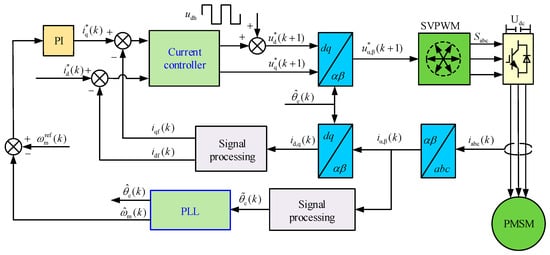
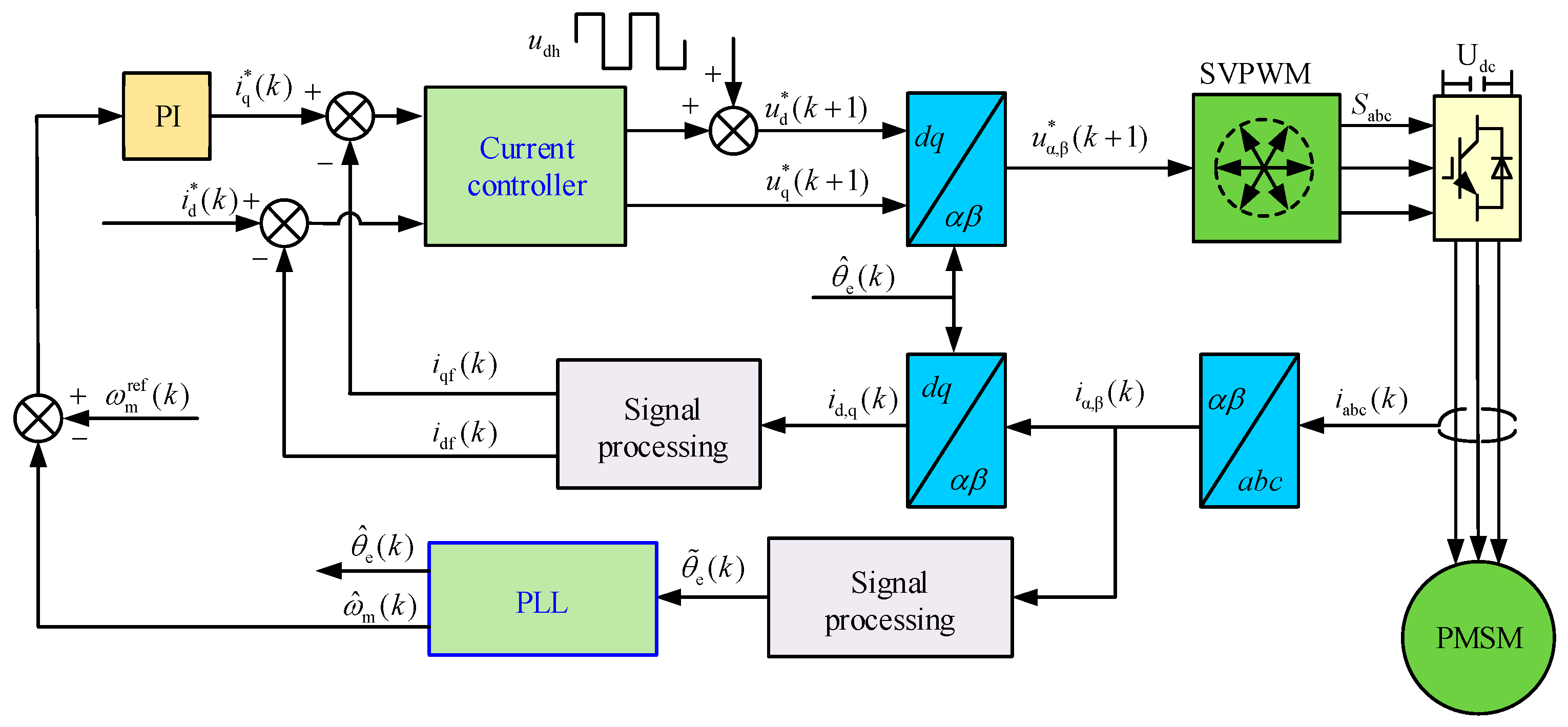
High-power motors with large inertia typically operate in the zero/low-speed region, making them suitable for high-frequency injection methods. The algorithm selected in this paper is HF-SWVI, and the system block diagram is shown in Figure 1. The system primarily consists of three components: the speed control loop, the current control loop, and the observer. The speed and current control loops generate the current reference and voltage reference, respectively, based on their corresponding set points and feedback values. The observer first processes the sampled current data and then estimates the rotor position and speed via a PLL. Therefore, the accuracy of the PLL estimation is crucial for the dynamic performance of the system. The operating principle of the PI-based PLL is analyzed below.

Figure 1. Block Diagram of the PMSM Position Sensorless Control System Based on HF-SWVI.

Since the frequency of the injected signal is much higher than the fundamental frequency during motor operation, voltage coupling terms, back-EMF, and phase resistance related to the fundamental frequency can be neglected. Thus, the mathematical model of the PMSM under high-frequency excitation is given as

$$\left[\begin{array}{l}{u}_{\mathrm{dh}}\\ u_{\mathrm{qh}}\end{array}\right]=\left[\begin{array}{cc}{L}_{\mathrm{d}}& 0\\ 0& L_{\mathrm{q}}\end{array}\right]\left[\begin{array}{l}p{i}_{\mathrm{dh}}\\ p{i}_{\mathrm{qh}}\end{array}\right].$$

(1)

where u_dh and u_qh are the high-frequency voltage components in the dq-axis frame; L_d and L_q are the d-axis and q-axis inductances, respectively; i_dh and i_qh are the high-frequency current components in the dq-axis frame; and p is the differential operator.

The d-axis injection method is adopted, and the injected square-wave voltage is expressed as

$$u_{\mathrm{dh}}=\left\{\begin{array}{l}{V}_{\mathrm{inj}},t\in [n{T}_{\mathrm{inj}},(n+{\displaystyle \frac{1}{2}})T_{\mathrm{inj}}]\\ -V_{\mathrm{inj}},t\in [(n+{\displaystyle \frac{1}{2}})T_{\mathrm{inj}},(n+1)T_{\mathrm{inj}}]\end{array}\right..$$

(2)

where V_inj is the amplitude of the square-wave voltage, T_inj is the injection period, and n is the number of injected periods. Substituting (2) into (1) and applying the inverse Park transform yields the high-frequency current response in the αβ-axis frame as

$$\left[\begin{array}{l}p{i}_{\mathsf{\alpha }\mathrm{h}}\\ p{i}_{\mathsf{\beta }\mathrm{h}}\end{array}\right]={\displaystyle \frac{V_{\mathrm{inj}}}{L_{\mathrm{d}}{L}_{\mathrm{q}}}}\left[\begin{array}{l}{L}_{\mathrm{d}}\sin {\theta }_{\mathrm{e}}\sin {\tilde{\theta }}_{\mathrm{e}}+L_{\mathrm{q}}\cos {\theta }_{\mathrm{e}}\cos {\tilde{\theta }}_{\mathrm{e}}\\ -L_{\mathrm{d}}\cos {\theta }_{\mathrm{e}}\sin {\tilde{\theta }}_{\mathrm{e}}+L_{\mathrm{q}}\sin {\theta }_{\mathrm{e}}\cos {\tilde{\theta }}_{\mathrm{e}}\end{array}\right].$$

(3)

where ${\tilde{\theta }}_{\mathrm{e}}={\theta }_{\mathrm{e}}-{\widehat{\theta }}_{\mathrm{e}}$ is the rotor position error, ${\theta }_{\mathrm{e}}$ is the actual rotor position and ${\widehat{\theta }}_{\mathrm{e}}$ is the estimated rotor position.

To derive a linearized PLL model for controller analysis and design, it is assumed that in steady state the estimated speed closely tracks the actual speed, making ${\tilde{\theta }}_{\mathrm{e}}$ negligible. Thus, the high-frequency current signal containing the actual rotor position can be derived as

$$\left[\begin{array}{l}p{i}_{\mathsf{\alpha }\mathrm{h}}\\ p{i}_{\mathsf{\beta }\mathrm{h}}\end{array}\right]={\displaystyle \frac{V_{\mathrm{inj}}}{L_{\mathrm{d}}}}\left[\begin{array}{l}\cos {\theta }_{\mathrm{e}}\\ \sin {\theta }_{\mathrm{e}}\end{array}\right].$$

(4)

The fundamental principle of the PI-based PLL is analyzed below. It consists of a phase detector (PD), a loop filter (LF), and a voltage-controlled oscillator (VCO). It takes the high-frequency current signal as its input and adjusts the angular frequency of the output signal through the LF. For the PD of the PLL, the relationship is expressed as

$$\epsilon ={\displaystyle \frac{L_{\mathrm{d}}}{V_{\mathrm{inj}}}}p{i}_{\mathsf{\beta }\mathrm{h}}\cdot \cos {\widehat{\theta }}_{\mathrm{e}}-{\displaystyle \frac{L_{\mathrm{d}}}{V_{\mathrm{inj}}}}p{i}_{\mathsf{\alpha }\mathrm{h}}\cdot \sin {\widehat{\theta }}_{\mathrm{e}}=\sin ({\theta }_{\mathrm{e}}-{\widehat{\theta }}_{\mathrm{e}}).$$

(5)

When the error is small,

$$\epsilon \approx {\theta }_{\mathrm{e}}-{\widehat{\theta }}_{\mathrm{e}}={\tilde{\theta }}_{\mathrm{e}}.$$

(6)

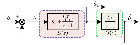
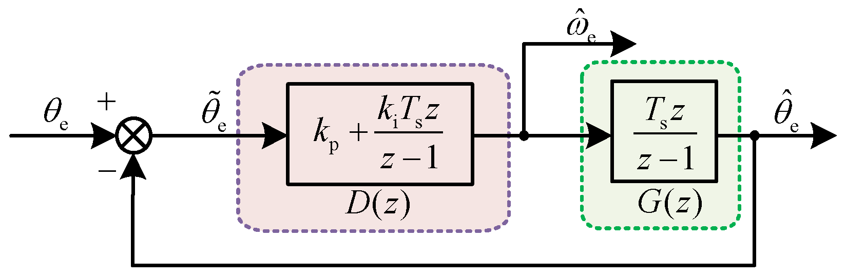
From (5) and (6), the schematic diagram of the PI-based PLL under square-wave injection can be derived, as shown in Figure 2. In Figure 2, k_p and k_i represent the proportional and integral gains; ${\widehat{\omega }}_{\mathrm{e}}$ is the estimated electrical angular velocity; and T_s is the sampling period of the discrete system.

Figure 2. Simplified Block Diagram of the Conventional PI-based PLL.

Based on Figure 2, the error transfer function of the PI-based PLL in the discrete domain can be derived as follows

$${\Phi }_{\mathrm{e}}(z)={\displaystyle \frac{{\tilde{\theta }}_{\mathrm{e}}(z)}{{\theta }_{\mathrm{e}}(z)}}={\displaystyle \frac{-1+2z^{-1}-z^{-2}}{(K_{\mathrm{P}}+K_{\mathrm{I}}+1)-(K_{\mathrm{p}}+2)z^{-1}+z^{-2}}}.$$

(7)

where K_p = k_pT_s and K_i = k_iT_s². During motor startup or upon sudden load connection, the rotor experiences significant angular acceleration, resulting in a linear-like increase or decrease in speed. Under this condition, the rotor position in the discrete domain is thus expressed as

$${\theta }_{\mathrm{e}}(z)={\displaystyle \frac{{\theta }_0}{z-1}}+{\displaystyle \frac{{\omega }_0{T}_{\mathrm{s}}z}{{(z-1)}^2}}+{\displaystyle \frac{a{T}_{\mathrm{s}}^{2}z(z+1)}{2{(z-1)}^3}}.$$

(8)

where θ₀ is the initial rotor position, ω₀ is the initial electrical angular velocity, and a is the electrical angular acceleration. Based on (7) and (8), the steady-state error of the rotor position estimation for the PI-based PLL during motor speed transients can be derived as

$${\tilde{\theta }}_{\mathrm{e}}(z)=\underset{z\to 1}{\lim }(z-1){\theta }_{\mathrm{e}}(z){\Phi }_{\mathrm{e}}(z)={\displaystyle \frac{a}{k_{\mathrm{i}}}}.$$

(9)

Equation (9) indicates that the conventional PI-based PLL exhibits a steady-state error during speed transients. Moreover, due to the inherent control characteristics of digital systems, the resulting voltage command exhibits a one-switching-period delay when implemented in PWM. At low switching frequencies, this delay occupies a significant portion of the motor’s electrical period. As the rotor continues to rotate during this delay, the reliability of the position estimation is further degraded. Additionally, this error is related to both the acceleration a and the integral gain ki. While increasing ki can reduce the position estimation error, it simultaneously introduces significant fluctuations in the estimated speed. Therefore, the PI-based PLL demonstrates clear limitations in speed estimation under low switching frequencies.

3. Principles and Parameter Design of DDCPLL

To address the limitations of the conventional PI-based PLL, a novel DDCPLL is designed directly in the discrete domain in this section. The design process involves two primary steps. First, a deadbeat controller is designed to eliminate the steady-state error. Then, based on this controller, a damping factor is introduced to ensure the stable operation of the position sensorless system. The detailed design procedure is as follows.

To facilitate implementation, the proposed PLL is designed with the same quadrature structure as the PI-based PLL, and its simplified block diagram retains the form shown in Figure 2. Consequently, the pulse transfer function of the deadbeat controller D_d(z) is given by

$$D_{\mathrm{d}}(z)={\displaystyle \frac{{\Phi }_{\mathrm{d}}(z)}{G(z)(1-{\Phi }_{\mathrm{d}}(z))}}={\displaystyle \frac{{\Phi }_{\mathrm{d}}(z)}{G(z){\Phi }_{\mathrm{ed}}(z)}}.$$

(10)

where Φ_d(z) represents the equivalent closed-loop pulse transfer function. When the rotor angular velocity undergoes a ramp change, the system error is given by

$${\tilde{\theta }}_{\mathrm{e}}(z)=\underset{z\to 1}{\lim }(z-1){\Phi }_{\mathrm{ed}}(z){\displaystyle \frac{a{T}_{\mathrm{s}}^{2}z(z+1)}{2{(1-z^{-1})}^3}}.$$

(11)

Equation (11) indicates that for the acceleration term ${\widehat{\theta }}_{\mathrm{e}}$ to fully converge to ${\theta }_{\mathrm{e}}$ following a speed transient, the error transfer function of the PLL must incorporate a third-order zero corresponding to the type of input signal. Therefore, the error pulse transfer function ${\Phi }_{\mathrm{ed}}(z)$ is designed as

$${\Phi }_{\mathrm{ed}}(z)=1-{\Phi }_{\mathrm{d}}(z)={(1-z^{-1})}^{3}F(z).$$

(12)

where F(z) is a polynomial that does not contain the factor (1 − z⁻¹) and is used to compensate for the poles of G(z) located outside the unit circle in the z-plane. Since the plant is an integral element, T_sz/(z − 1), the pulse transfer function of the deadbeat controller can be derived from (10) as follows:

$$D_{\mathrm{d}}(z)={\displaystyle \frac{1-{(1-z^{-1})}^3}{\frac{T_{\mathrm{s}}z}{z-1}\cdot {(1-z^{-1})}^3}}={\displaystyle \frac{3z^2-3z+1}{T_{\mathrm{s}}(z^3-2z^2+z)}}.$$

(13)

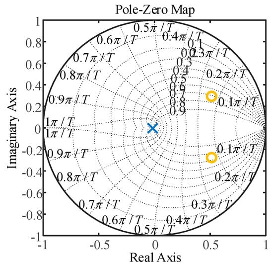
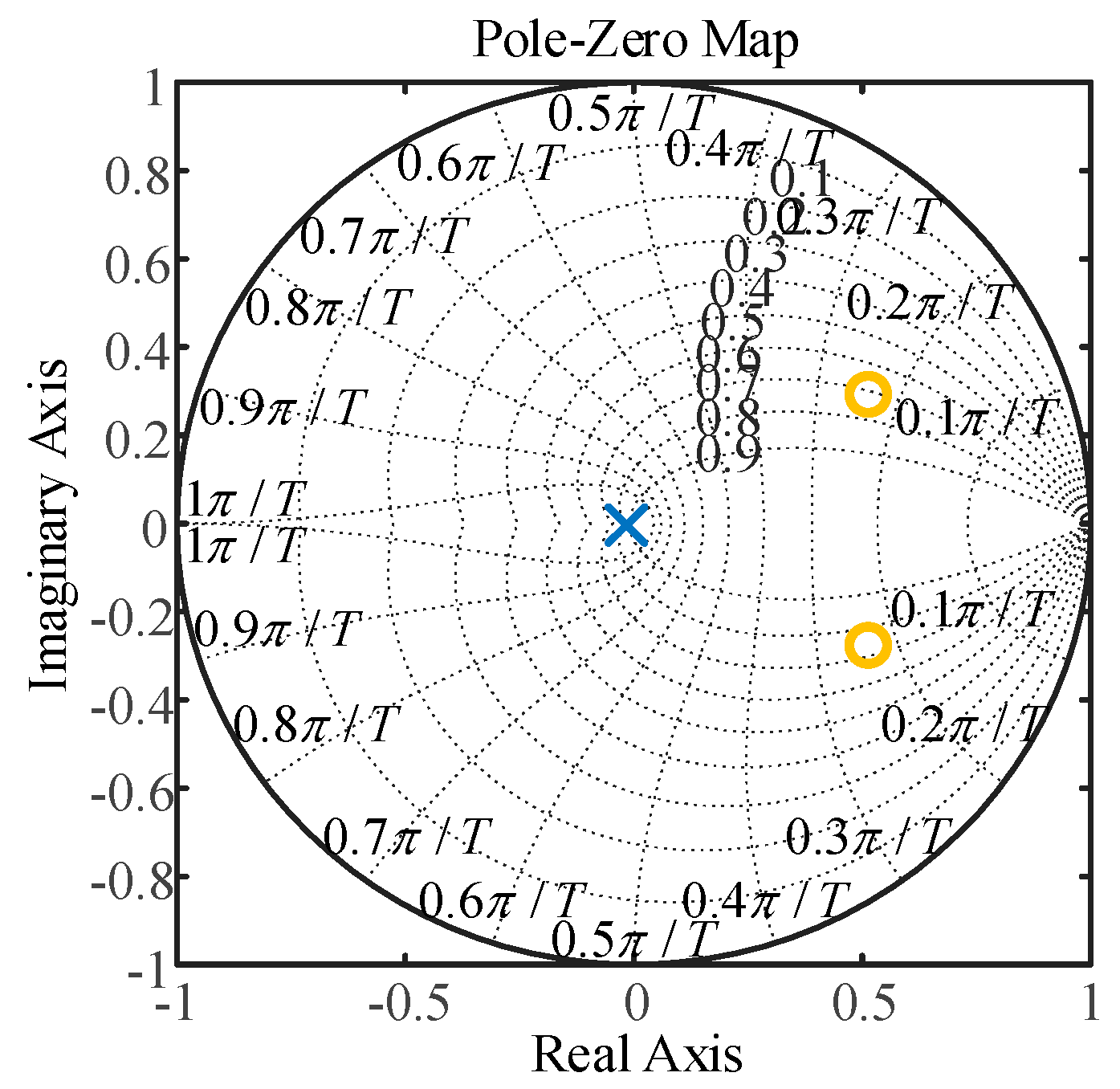
With the controller described by (13), the zeros and poles of the PLL’s equivalent closed-loop pulse transfer function are plotted in Figure 3. As shown, all system poles lie inside the unit circle, indicating that the system is stable.

Figure 3. Pole-Zero Plot of the Deadbeat PLL.

On the basis of system stability, the steady-state error can be further calculated as

$${\tilde{\theta }}_{\mathrm{e}}(z)=\underset{z\to 1}{\lim }(z-1){\displaystyle \frac{\frac{a{T}_s^{2}z(z+1)}{2}}{{(1-z^{-1})}^3}}{(1-z^{-1})}^3=0.$$

(14)

A comparison between (9) and (14) reveals that employing a deadbeat controller enables accurate estimation of the actual rotor position during speed transients.

However, as can be observed from Figure 3, all poles of the closed-loop pulse transfer function are placed at the origin of the z-plane. While this configuration ensures the highest theoretically achievable response speed, the resulting rapid dynamic response implies large control efforts. It is noteworthy from Figure 1 that the controller’s output is the estimated speed. In the implementation of sensorless algorithms, this estimated speed serves as the feedback signal for the speed control loop and is therefore critical for the stable operation of the sensorless system. Consequently, after achieving accurate rotor position estimation, it becomes imperative to further ensure the smoothness of the control effort.

To address this issue, this section introduces a damping factor by adding an additional pole into the closed-loop system. To maintain system stability and avoid ringing after the introduction of this new pole, it is placed on the positive real axis within the z-plane. This modification changes the theoretical system response from a finite settling time to an exponentially decaying one. The new error pulse transfer function ${\Phi }_{\mathrm{ea}}(z)$ of the system after introducing this pole is given as

$${\Phi }_{\mathrm{ea}}(z)={\displaystyle \frac{{\Phi }_{\mathrm{ed}}}{1-\lambda z^{-1}}}={\displaystyle \frac{{(z-1)}^3}{z^2(z-\lambda )}}.$$

(15)

where λ is the damping factor with λ > 0. From (10), (12), and (15), the equivalent closed-loop pulse transfer function ${\Phi }_{\mathrm{a}}(z)$ and the controller pulse transfer function $D_{\mathrm{a}}(z)$ of the proposed DDCPLL incorporating λ can be derived as

$${\Phi }_{\mathrm{a}}(z)={\displaystyle \frac{{\Phi }_{\mathrm{d}}(z)-\lambda z^{-1}}{1-\lambda z^{-1}}}={\displaystyle \frac{(3-\lambda )z^2-3z+1}{z^2(z-\lambda )}}.$$

(16)

$$D_{\mathrm{a}}(z)={\displaystyle \frac{(3-\lambda )z^2-3z+1}{T_s(z^3-2z^2+z)}}.$$

(17)

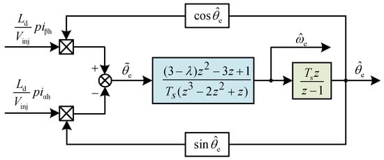
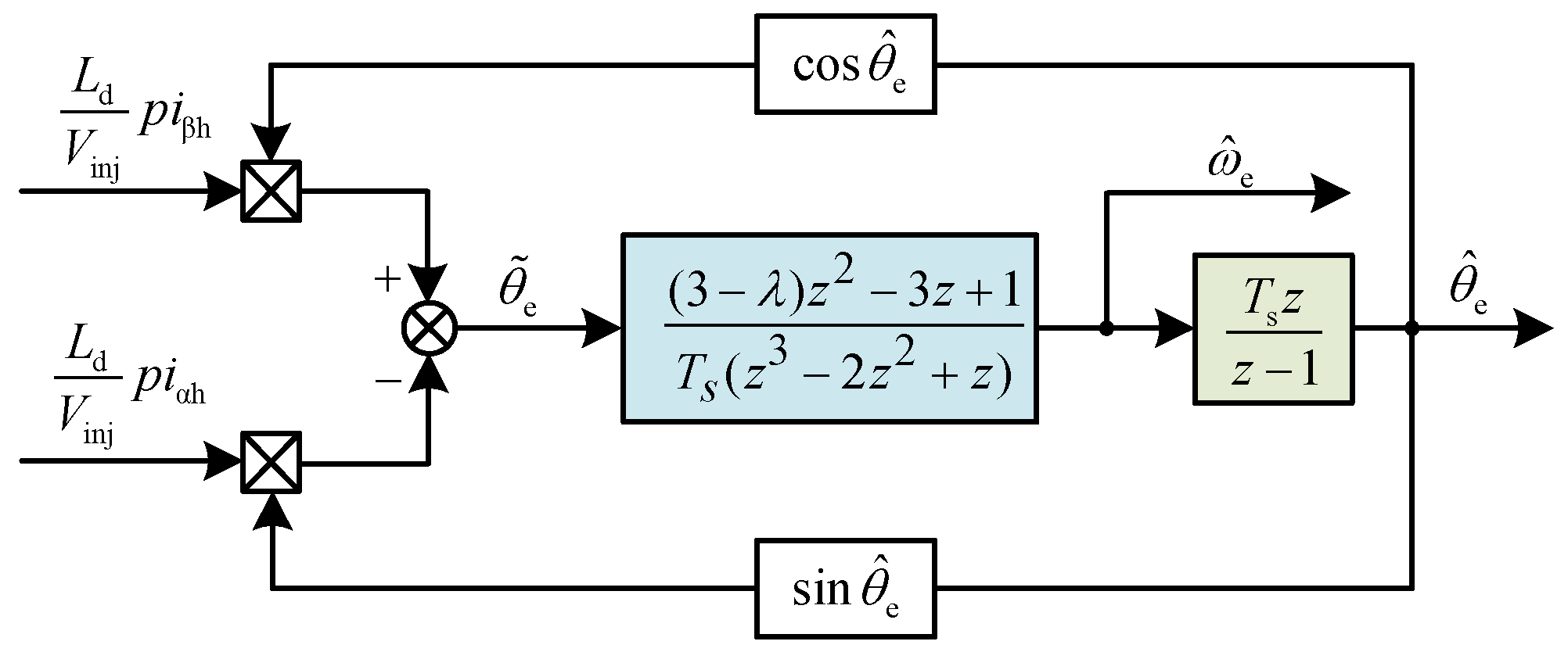
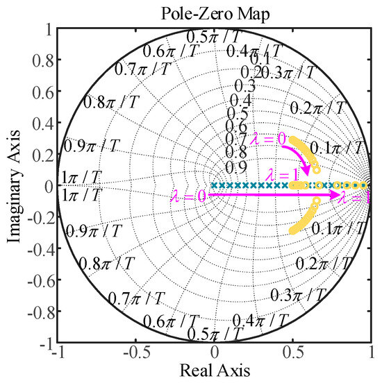
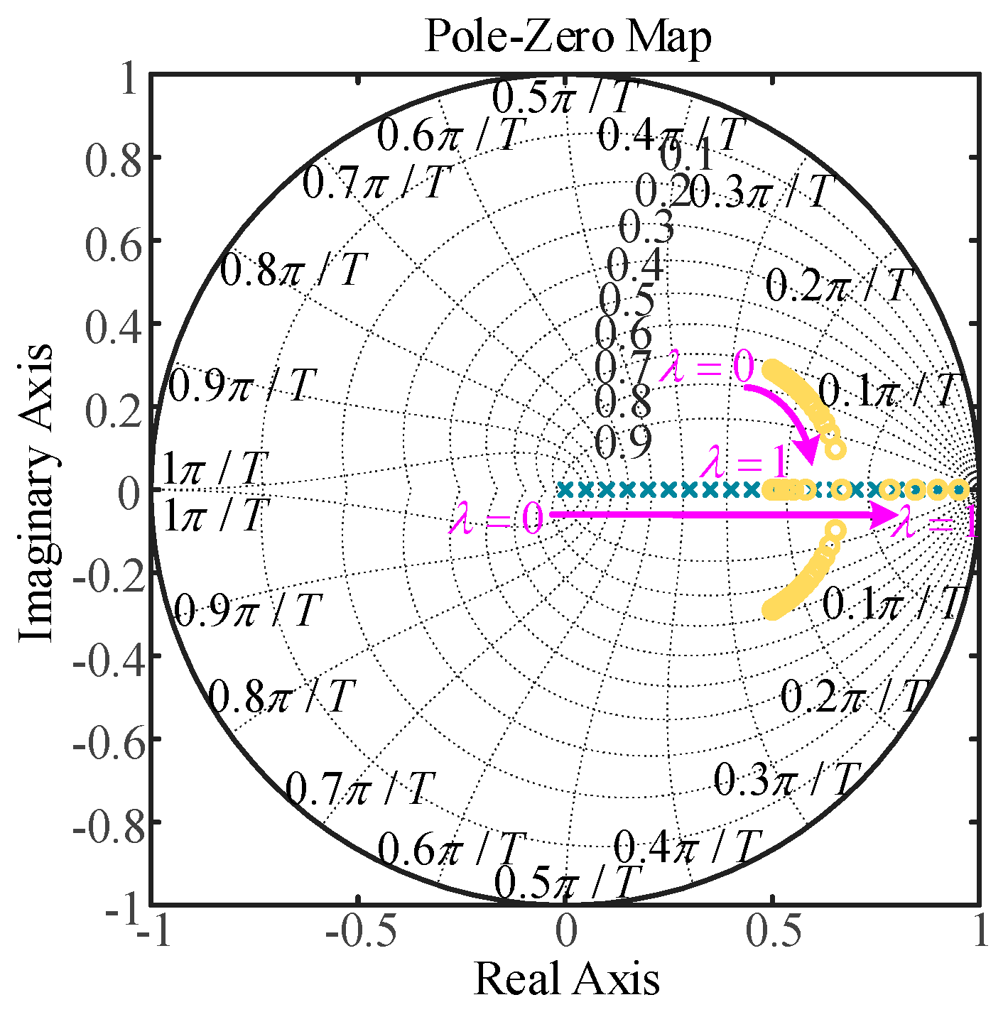
Based on the foregoing analysis, the schematic diagram of the DDCPLL can be summarized as shown in Figure 4. Starting with an initial value of λ = 0 and incrementing it gradually with a step size of 0.05, the movement of the zeros and poles of the DDCPLL’s equivalent closed-loop pulse transfer function with respect to λ is illustrated in Figure 5.

Figure 4. Block Diagram of the DDCPLL.

Figure 5. Pole-Zero Plot of the DDCPLL (λ:0→1).

Figure 5 reveals that the system poles always lie on the positive real axis within the z-plane. As λ increases, these poles move closer to the unit circle boundary. This indicates a continuous reduction in the system’s stability margin, resulting in a slower dynamic response and a significantly increased settling time. The system reaches a critically stable state when λ = 1. Further increase in λ beyond this point leads to instability; therefore, λ must be constrained to values less than 1. Initially, the system zeros are complex conjugates located symmetrically about the real axis in the right-half plane, endowing the system with non-minimum phase characteristics. This leads to overshoot and oscillatory behavior in its step response. As λ increases, the zeros migrate toward the real axis, their imaginary parts diminish, and the oscillatory effect caused by the complex zeros gradually weakens. Once the zeros completely settle onto the real axis, the oscillatory component in the response vanishes, and the waveform becomes monotonic. In summary, the evolution of the zeros and poles demonstrates that introducing the damping factor λ can effectively suppress control effort overshoot, thereby achieving a smoother estimated speed. This smoothing effect becomes more pronounced with larger λ values. However, it is crucial to note that λ must remain less than 1 to prevent system instability.

Following the qualitative analysis of the effect of λ, the effect of λ on the rotor position estimation error is quantitatively investigated below. To conveniently obtain the sequence of the rotor position estimation error, (11) can be rearranged into the following form

$$\begin{array}{l}{\tilde{\theta }}_{\mathrm{e}}(z)={\Phi }_e(z){\displaystyle \frac{a{T}_{\mathrm{s}}^{2}z(z+1)}{2{(1-z^{-1})}^3}}\\ =-{\displaystyle \frac{a{T}_s^2}{2\lambda }}{z}^{-1}+{\displaystyle \frac{a{T}_s^2(\lambda +1)}{2\lambda }}{\displaystyle \sum _{k=0}^{\infty }{\lambda }^k{z}^{-(k+1)}}.\end{array}$$

(18)

Consequently, the rotor position error sequence can be derived from (18) as

$${\tilde{\theta }}_e[k]=\left\{\begin{array}{l}0,k=0\\ 0.5a{T}_s^2,k=1\\ 0.5a{T}_s^2({\lambda }^{k-1}+{\lambda }^{k-2}),k\ge 2\end{array}\right..$$

(19)

Equation (19) reveals that, starting from the second sampling instant, the rotor position estimation error sequence decays exponentially to zero. Furthermore, a larger damping factor corresponds to a slower decay rate. When λ = 1, the DDCPLL is in a critically stable state, the error sequence converges to a non-zero constant. If λ > 1, the error diverges exponentially, leading to system instability. These results are fully consistent with the conclusions drawn from the qualitative analysis. Additionally, it can be inferred that the selection of λ is constrained by the electrical angular acceleration, the switching period, and the acceptable level of angular error.

Based on the above analysis, to comprehensively consider the dynamic performance and noise immunity indicators, we adopt a multi-objective optimization method. Combining the two indicators, the cost function $J(\lambda )$ is defined as

$$J(\lambda )=\alpha f_1(\lambda )+\beta f_2(\lambda )={\displaystyle \frac{\alpha }{1-\lambda }}+{\displaystyle \frac{\beta }{\lambda }},\lambda \in (0,1).$$

(20)

In (20) α, β > 0 are weight coefficients, reflecting the importance attached to dynamic performance and noise immunity performance. To find the λ that minimizes the cost function, differentiate (20) and set the derivative to zero to obtain

$$\lambda ={\displaystyle \frac{\sqrt{\beta /\alpha }}{1+\sqrt{\beta /\alpha }}}.$$

(21)

If there are higher requirements for a certain performance in practical applications, adjustments can be made according to (21), combined with experimental fine-tuning.

4. Precise Discrete-Domain Modeling and Closed-Loop Controller Parameter Design of the Position Sensorless System Incorporating DDCPLL

At low switching frequency, the control systems exhibit a large control delay. This leads to a considerable discrepancy between the actual control performance and the expected performance when using controller parameters designed based on a continuous-time domain system model. To address this issue, this section establishes a relatively precise discrete-domain model of each component of the system. Based upon this model, the control parameters for both the current loop and the speed loop are optimized to significantly increase the dynamic performance.

4.1. Discrete-Domain Modeling of PMSM

Researchers have derived a discrete-domain model for PMSM based on the motor’s complex vector equations [24]. The detailed derivation process is as follows.

Under ideal conditions, the voltage equations of a PMSM in the dq-axis frame can be expressed as

$$\begin{gathered} \left[\begin{array}{l}{u}_{\mathrm{d}}\\ u_{\mathrm{q}}\end{array}\right]=\left[\begin{array}{cc}{R}_{\mathrm{s}}+p{L}_{\mathrm{d}}& -{\omega }_{\mathrm{e}}{L}_{\mathrm{q}}\\ {\omega }_{\mathrm{e}}{L}_{\mathrm{q}}& R_{\mathrm{s}}+p{L}_{\mathrm{d}}\end{array}\right]\left[\begin{array}{l}{i}_{\mathrm{d}}\\ i_{\mathrm{d}}\end{array}\right] \\ +\left[\begin{array}{l}0\\ (L_{\mathrm{d}}-L_{\mathrm{q}})({\omega }_{\mathrm{e}}{i}_{\mathrm{d}}-p{i}_{\mathrm{q}})+{\omega }_{\mathrm{e}}{\psi }_{\mathrm{f}}\end{array}\right]. \end{gathered}$$

(22)

where u_d and u_q represent the stator voltages in the dq-axis frame, i_d and i_q denote the stator currents in the dq-axis frame, R_s is the phase resistance, ω_e is the electrical angular velocity, and ψ_f is the permanent magnet flux linkage. The extended electromotive force (EEMF) of the PMSM is defined as E, whose expression is given by

$$E=(L_{\mathrm{d}}-L_{\mathrm{q}})({\omega }_{\mathrm{e}}{i}_{\mathrm{d}}-p{i}_{\mathrm{q}})+{\omega }_{\mathrm{e}}{\psi }_{\mathrm{f}}.$$

(23)

The motor model based on the EEMF, derived from (22) and (23), is expressed in complex vector form as

$$\begin{array}{l}{\mathit{u}}_{\mathrm{dq}}=(R_{\mathrm{s}}+p{L}_{\mathrm{d}}+j{\omega }_{\mathrm{e}}{L}_{\mathrm{q}}){\mathit{i}}_{\mathrm{qd}}+{\mathit{e}}_{\mathrm{dq}}\\ {\mathit{e}}_{\mathrm{dq}}=jE=j[(L_{\mathrm{d}}-L_{\mathrm{q}})({\omega }_{\mathrm{e}}{i}_{\mathrm{d}}-p{i}_{\mathrm{q}})+{\omega }_{\mathrm{e}}{\psi }_{\mathrm{f}}].\end{array}$$

(24)

Rewriting the PMSM complex vector model given in (24) into the form of a differential equation yields

$${\mathit{i}}_{\mathrm{dq}}+{\displaystyle \frac{L_{\mathrm{d}}}{R_{\mathrm{s}}+j{\omega }_{\mathrm{e}}{L}_{\mathrm{q}}}}p{\mathit{i}}_{\mathrm{dq}}={\displaystyle \frac{1}{R_{\mathrm{s}}+j{\omega }_{\mathrm{e}}{L}_{\mathrm{q}}}}({\mathit{u}}_{\mathrm{dq}}-{\mathit{e}}_{\mathrm{dq}}).$$

(25)

Solving (25) with the initial current set as i_dq(t₀), the complex vector current i_dq(t) at time t can be obtained as

$$\begin{array}{l}{\mathit{i}}_{\mathrm{dq}}(t)=e^{-{\displaystyle \frac{R_{\mathrm{s}}+j{\omega }_{\mathrm{e}}{L}_{\mathrm{q}}}{L_{\mathrm{d}}}}(t-t_0)}{\mathit{i}}_{\mathrm{dq}}(t_0)\\ +{\displaystyle \frac{1}{L_{\mathrm{d}}}}{\displaystyle {\int }_{t_0}^t{e}^{-\frac{R_{\mathrm{s}}+j{\omega }_{\mathrm{e}}{L}_{\mathrm{q}}}{L_{\mathrm{d}}}(t-\tau )}}[{\mathit{u}}_{\mathrm{dq}}(t)-{\mathit{e}}_{\mathrm{dq}}(t)]d\tau .\end{array}$$

(26)

To simplify the integration in (26), the following reasonable assumptions can be made: the motor speed remains constant between two sampling instants, and the extended back-EMF remains constant during this interval. Secondly, the voltage vector output by the inverter is considered constant within one control period. In practical applications, the back-EMF can be treated as a disturbance [25]. Furthermore, considering the one-sample computational delay inherent in the digital implementation of PWM updating, the discrete-domain mathematical model of the PMSM can be derived as

$${\displaystyle \frac{{\mathit{i}}_{\mathrm{dq}}(z)}{{\mathit{u}}_{\mathrm{dq}}(z)}}={\displaystyle \frac{e^{-j{\omega }_{\mathrm{e}}{T}_{\mathrm{s}}}-e^{-\frac{R_{\mathrm{s}}+j{\omega }_{\mathrm{e}}{L}_{\mathrm{q}}}{L_{\mathrm{d}}}{T}_{\mathrm{s}}}}{z{e}^{j{\omega }_{\mathrm{e}}{T}_{\mathrm{s}}}[R_{\mathrm{s}}-j{\omega }_{\mathrm{e}}(L_{\mathrm{q}}-L_{\mathrm{d}})](z-e^{-\frac{R_{\mathrm{s}}+j{\omega }_{\mathrm{e}}{L}_{\mathrm{q}}}{L_{\mathrm{d}}}{T}_{\mathrm{s}}})}}.$$

(27)

From (27), it can be seen that the motor model contains a speed-dependent factor R_s − jω_e(L_q − L_d). It is worth noting that large-inertia motors generally operate at low speeds and have very small inductances. Therefore, the imaginary part related to speed in this factor can be neglected. Furthermore, it can be observed from the transfer function that the inductance values in the numerator and denominator of the exponential term differ. To further simplify the analysis and achieve pole-zero cancellation, this paper adopts an average inductance approximation, resulting in

$$G_{\mathrm{pdq}}(z)={\displaystyle \frac{{\mathit{i}}_{\mathrm{dq}}(z)}{{\mathit{u}}_{\mathrm{dq}}(z)}}={\displaystyle \frac{e^{-j{\omega }_{\mathrm{e}}{T}_{\mathrm{s}}}-e^{-\frac{R_{\mathrm{s}}+j{\omega }_{\mathrm{e}}L}{L}{T}_{\mathrm{s}}}}{z{e}^{j{\omega }_{\mathrm{e}}{T}_{\mathrm{s}}}{R}_{\mathrm{s}}(z-e^{-\frac{R_{\mathrm{s}}+j{\omega }_{\mathrm{e}}L}{L}{T}_{\mathrm{s}}})}}$$

(28)

where L is average inductance, L = (L_d + L_q)/2.

4.2. Current Controller Design

Based on the derived motor model, a current controller is designed directly in the discrete domain in this section. For analytical convenience, (28) is rewritten as

$$G_{\mathrm{pdq}}(z)={\displaystyle \frac{{\mathit{i}}_{\mathrm{dq}}(z)}{{\mathit{u}}_{\mathrm{dq}}(z)}}={\displaystyle \frac{z^{-2}}{e^{j2{\omega }_{\mathrm{e}}{T}_{\mathrm{s}}}A(z)}}.$$

(29)

In (20), A(z) is

$$A(z)={\displaystyle \frac{R_{\mathrm{s}}}{1-e^{-\frac{R_{\mathrm{s}}}{L}{T}_{\mathrm{s}}}}}[1-z^{-1}{e}^{-({\displaystyle \frac{R_{\mathrm{s}}}{L}}+j{\omega }_{\mathrm{e}})T_{\mathrm{s}}}].$$

(30)

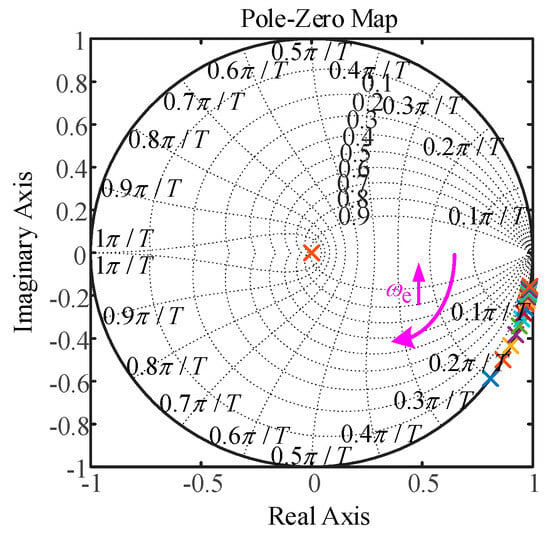
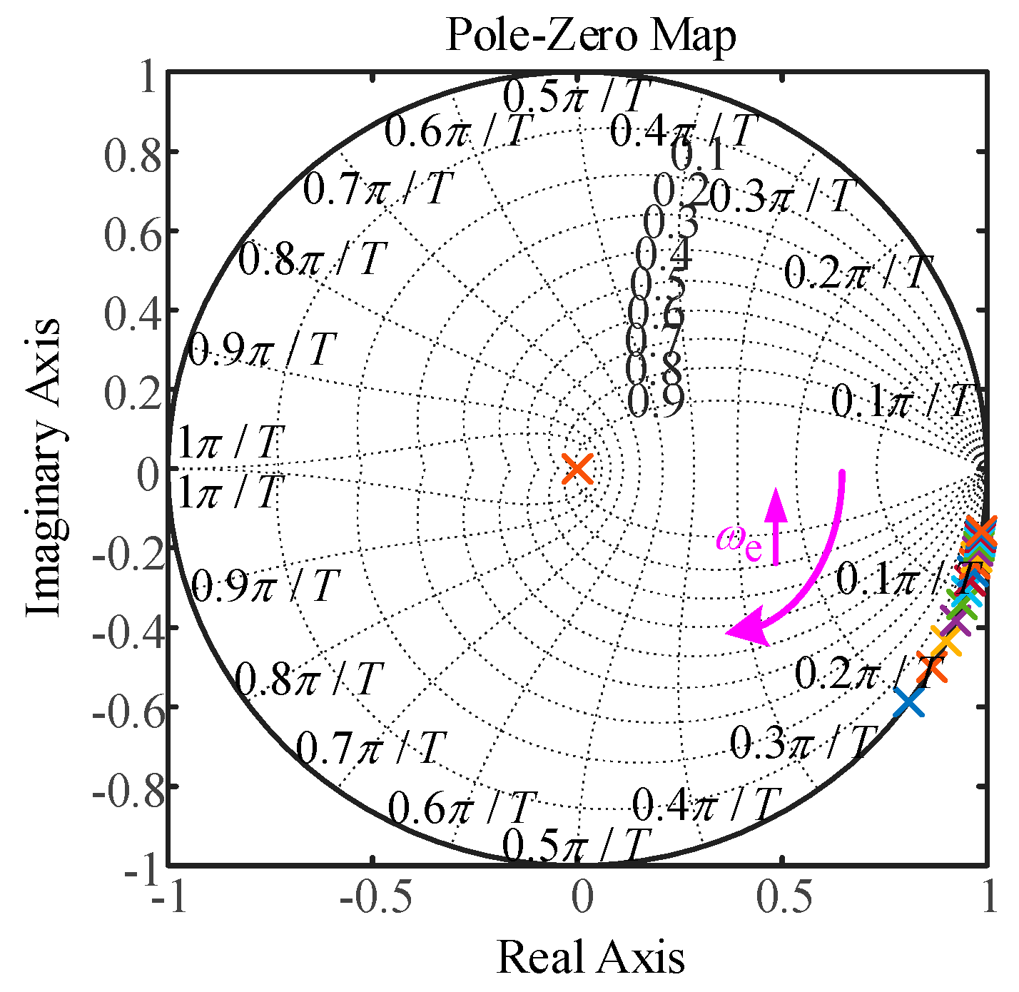
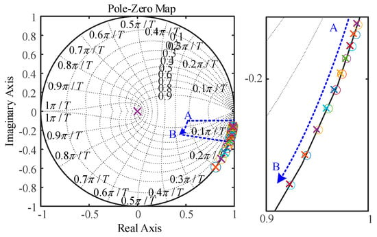
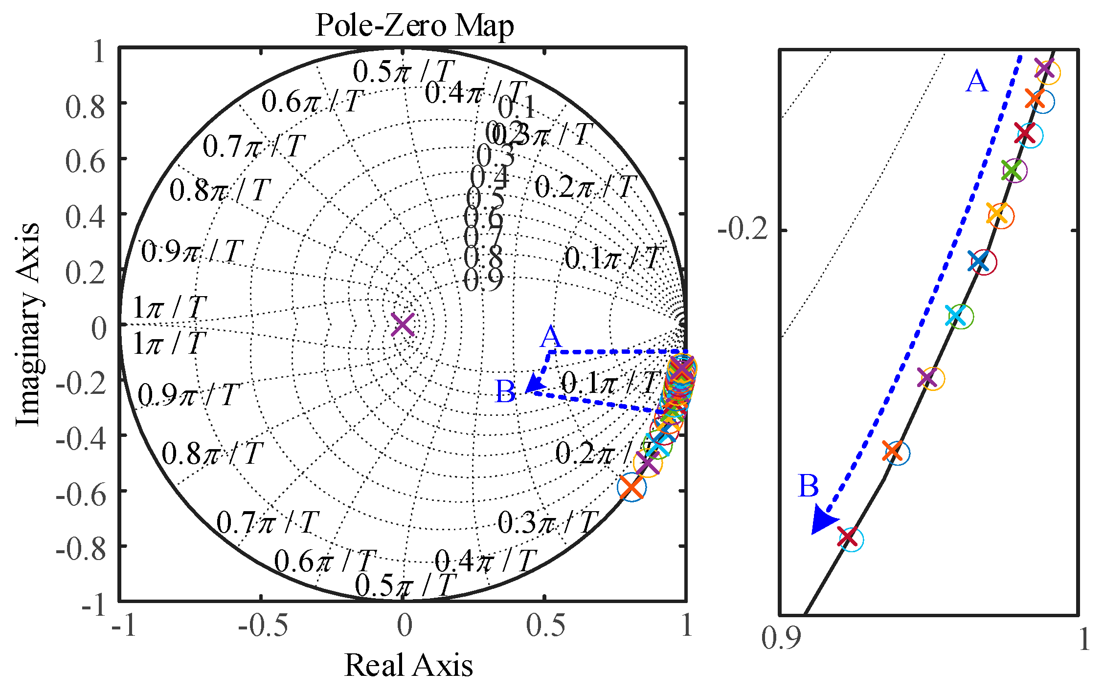
Figure 6 illustrates the migration of the poles of G_pdq(z) as the speed increases, under a fixed switching frequency. It can be observed from Figure 6 that the poles of G_pdq(z) move towards the left-half plane with increasing speed, indicating that the system’s oscillation frequency is progressively elevated. Conventional methods fail to strictly remove the poles of G_pdq(z) due to discretization errors, which is the fundamental reason why they are unsuitable for low switching frequency applications.

Figure 6. Pole Plot of PMSM.

Based on the above analysis and (29), the current controller can be designed according to the zero-pole principle as follows.

$$G_{\mathrm{c}}(z)={\displaystyle \frac{\gamma z}{z-1}}{z}^{-2}{G}_{\mathrm{pdq}}{(z)}^{-1}={\displaystyle \frac{\gamma z}{z-1}}{e}^{j2{\omega }_{\mathrm{e}}{T}_{\mathrm{s}}}A(z).$$

(31)

where γ is the design parameter. Combining (29) and (31), the closed-loop transfer function of the current loop with the designed current controller can be derived as

$$G(z)={\displaystyle \frac{{\mathit{i}}_{\mathrm{dq}}(z)}{{\mathit{i}}_{\mathrm{dq}}^{\ast }(z)}}={\displaystyle \frac{C_{\mathrm{c}}(z)G_{\mathrm{pdq}}(z)}{1+C_{\mathrm{c}}(z)G_{\mathrm{pdq}}(z)}}={\displaystyle \frac{\gamma }{z^2-z+\gamma }}.$$

(32)

From Equations (29)–(32), it can be observed that when the resistance and inductance parameters adopted in the current controller exactly match those of the actual motor, the zeros of the current controller can completely cancel the motor poles that shift with speed, thereby decoupling the control performance from speed variations. However, it should be noted that the current controller is designed based on the simplified motor model given in (28); therefore, the resistance and inductance values used in the controller inevitably differ from the actual parameters. Figure 7 illustrates the variation in the poles and zeros of both the current controller and the motor with respect to speed when the resistance ${\widehat{R}}_{\mathrm{s}}$ and inductance $\widehat{L}$ in the controller deviate from the actual values.

Figure 7. Movement of motor poles and current controller zeros with speed (${\widehat{R}}_{\mathrm{s}}=0.7R_{\mathrm{s}}, \widehat{L}=1.3L$).

It can be observed from Figure 7 that even when discrepancies exist in resistance and inductance, the motor and the current controller can still achieve satisfactory pole-zero cancellation, which demonstrates the feasibility of the controller design process and also indicates that the designed current controller possesses good robustness.

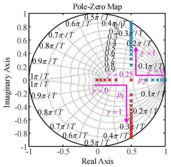
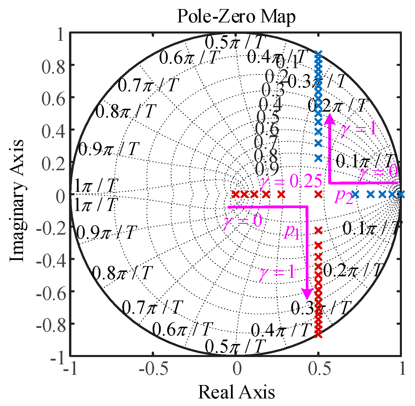
Equation (32) indicates that the characteristic equation of G(z) contains only one undetermined coefficient γ. Therefore, the dynamic response of the current loop is solely determined by γ. As shown in Figure 8, which illustrates the pole migration, setting γ = 0.25 ensures a fast response without overshoot. Consequently, γ is set to 0.25.

Figure 8. Pole-Zero Plot of the Current Loop (γ:0 → 1).

4.3. Speed Loop Modeling

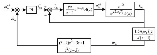
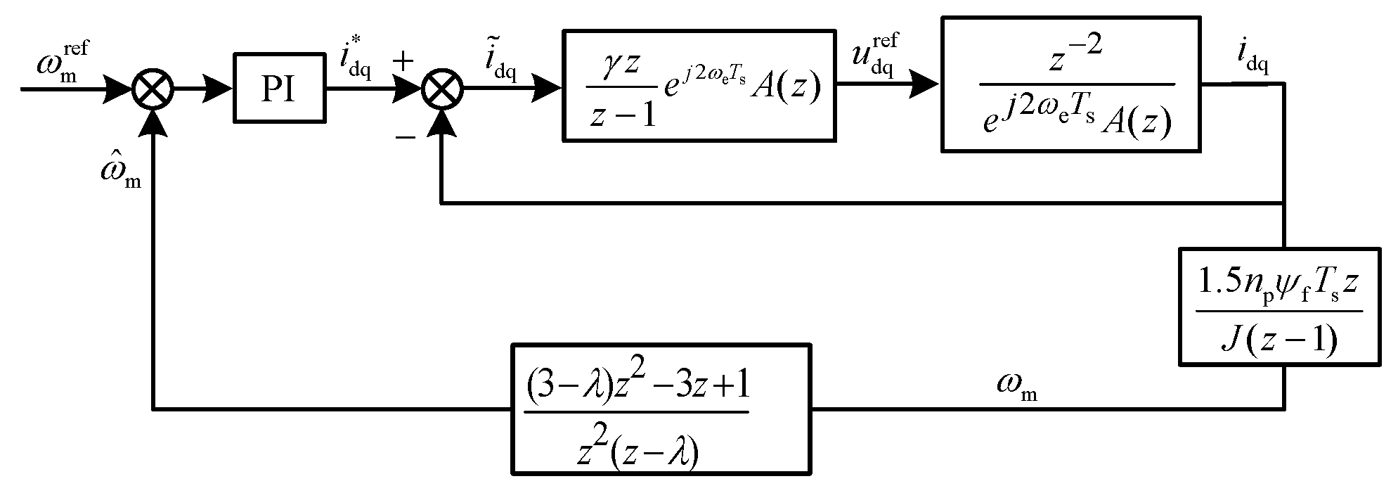
After designing the speed feedback loop and the current control loop, the overall control schematic is obtained as shown in Figure 9. The speed loop employs a PI controller, and its parameter tuning process is described as follows. The parameters of the motor control system used in the parameter tuning process of this section are listed in Table 1.

Figure 9. Speed Loop Control Schematic.

Table 1. Motor Parameters.

Parameter	Value
Phase resistance/Rs	0.257 mΩ
d-axis inductance/Ld	0.104 mH
q-axis inductance/Lq	0.156 mH
Rated frequency/fN	96 Hz
Rated speed/nN	640 rmp
Rated current/IN	7270 A_rms
Moment of inertia/J	750 (kg.m2)
Rated torque/TN	129.5 k (N.m)
Current controller parameter/γ	0.25
PLL parameter/λ	0.5
Switching frequency/fs	2000 Hz

By organizing the key components in Figure 9 and substituting the parameters from Table 1, the closed loop pulse transfer function $G_{\mathrm{p}}$ of the controlled plant is obtained as

$$G_{\mathrm{p}}={\displaystyle \frac{1.5n_{\mathrm{p}}{\psi }_{\mathrm{f}s}{T}_{\mathrm{s}}\gamma z}{J(z^2-z+\gamma )(z-1)}}={\displaystyle \frac{0.00000228z}{{(z-0.5)}^2(z-1)}}.$$

(33)

From (33), it can be seen that the controlled plant is a third-order system with a relatively complex expression. By retaining its dominant poles and matching the velocity error constant, the expression can be simplified to

$$G_{\mathrm{p}}\approx {\displaystyle \frac{0.00000912}{z-1}}.$$

(34)

Following the same approach, the simplified transfer function of the speed feedback loop can be derived as

$$G_{\mathrm{g}}\approx {\displaystyle \frac{0.5}{z-0.5}}.$$

(35)

This paper employs the pole placement method to determine the parameters. The desired dominant poles are chosen corresponding to a continuous-time second order system with a damping ratio of 0.7 and a natural frequency of 65.7 rad/s. The resulting second order factor mapped to the z plane is given as

$$z_{1,2}=0.9773\pm j0.02296.$$

(36)

The PI controller is discretized using the backward Euler method for its integral part. Substituting (36) into the closed-loop characteristic equation of the system and rearranging yields

$$\left\{\begin{array}{l}{K}_{\mathrm{P}}=4587\\ K_{\mathrm{i}}=21138\\ K_{\mathrm{i}}{T}_{\mathrm{s}}=10.569\end{array}\right..$$

(37)

Due to non-ideal factors causing errors between the measured and estimated speeds, it is necessary to analyze system robustness. Let Δω denote the external disturbance superimposed on the DDCPLL estimated speed. The transfer function from the reference speed to the actual speed, denoted as $T(z)$, and the transfer function from the disturbance to the actual speed, denoted as $S_{\mathrm{d}}(z)$, are given by

$$T(z)={\displaystyle \frac{\omega (z)}{{\omega }_{\mathrm{m}}^{\mathrm{ref}}(z)}}={\displaystyle \frac{G_{\mathrm{m}}(z)G_{\mathrm{c}}(z)C(z)}{1+G_{\mathrm{m}}(z)G_{\mathrm{c}}(z)C(z)H(z)}}$$

(38)

$$S_{\mathrm{d}}(z)={\displaystyle \frac{\omega (z)}{\Delta \omega (z)}}=-{\displaystyle \frac{G_{\mathrm{m}}(z)G_{\mathrm{c}}(z)C(z)}{1+G_{\mathrm{m}}(z)G_{\mathrm{c}}(z)C(z)H(z)}}.$$

(39)

It can be seen from (38) that the characteristic equation of the system does not contain Δω. Therefore, the steady-state error does not affect the distribution of the closed-loop poles, and the system stability remains unchanged. However, the steady-state accuracy is affected. Assuming the reference is a step signal of magnitude ωref,ss and the disturbance Δω is a constant value Δωss, using the final value theorem, we can obtain steady-state error e_ss as

$$e_{\mathrm{ss}}=\underset{z\to 1}{\lim }(z-1)({\omega }_{\mathrm{m}}^{\mathrm{ref}}(z)-\omega (z))=(1-T(1)){\omega }_{\mathrm{ref},\mathrm{ss}}+T(1)\Delta {\omega }_{\mathrm{ss}}=\Delta {\omega }_{\mathrm{ss}}.$$

(40)

Considering a specific transient disturbance: let the disturbance be a unit impulse signal, i.e., Δω(k) = δ(k). The resulting output deviation is the impulse response h_d(k). The disturbance transfer function S_d(z) can be expanded into a partial fraction form. Since all poles of the system are real, let the poles be p₁,p₂,…, p_n, and denote the magnitude of the dominant pole pd as r. The impulse response can then be expressed as

$$h_{\mathrm{d}}(k)={\displaystyle \sum _{i=1}^n{A}_{\mathrm{i}}{p}_{\mathrm{i}}^{\mathrm{k}}}.$$

(41)

When k is relatively large, the dominant pole plays a major role, yielding

$$\left|h_{\mathrm{d}}(k)\right|\approx \left|A_{\mathrm{d}}\right|r^k.$$

(42)

In summary, neither steady-state nor transient speed estimation errors affect the closed-loop stability of the system. The magnitudes of all closed-loop poles are less than 1, ensuring asymptotic stability. A constant disturbance Δωss leads to a speed static error of Δωss, but this error is negligible in practical systems. The damping factor λ controls the decay rate of the system’s response to transient disturbances by adjusting the magnitude r of the closed-loop dominant pole. A smaller λ results in faster decay and stronger suppression capability. However, in addition to speed estimation errors, practical systems may also face issues such as current sampling delay and high-frequency noise, which can be addressed through fixed delay compensation and adaptive filtering. Given the abundance of existing research on these topics and the focus of this paper on dynamic performance improvement, these issues are not discussed further.

5. System Performance Verification

Considering the megawatt-level power rating of the system, Hardware in the Loop (HIL) testing is adopted in this paper to reduce verification complexity and validate the performance of the proposed DDCPLL and control strategy. The specific tool used was Typhoon HIL, a platform capable of emulating the behavior of high-power permanent magnet synchronous motors and their drive systems with high fidelity, while accurately reflecting the execution effect of the controller code. This provides a testing environment close to actual operating conditions for algorithm validation. The motor control system parameters used are listed in Table 1.

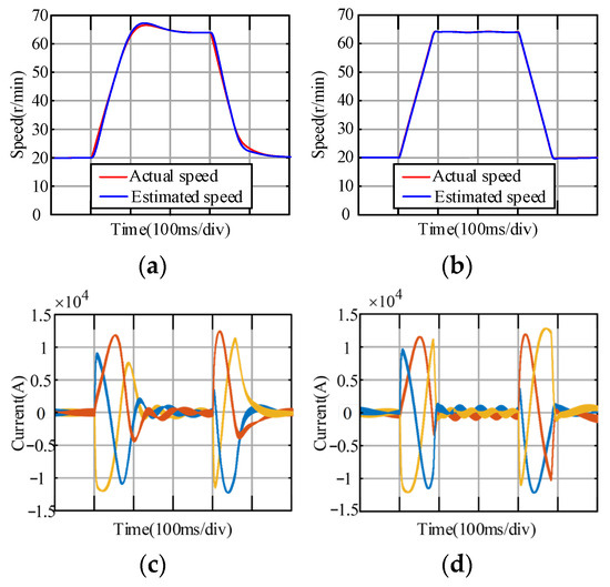
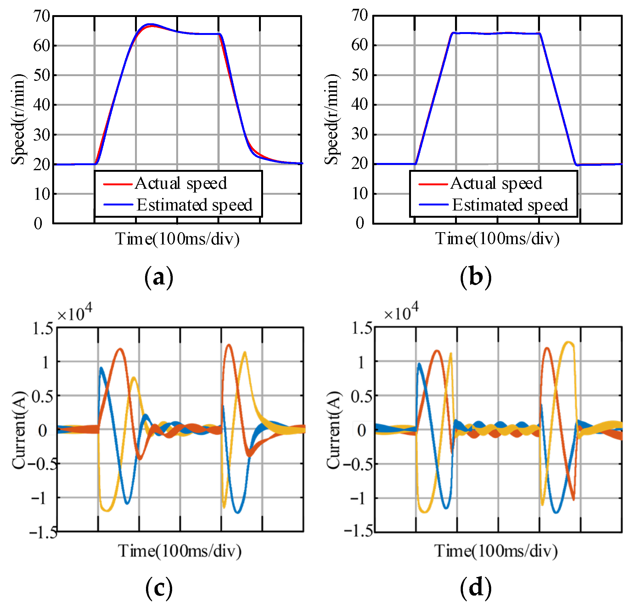
Figure 10 shows a performance comparison between the conventional control strategy with the PI-based PLL and the proposed strategy under the rotor speed references step conditions. Figure 10a,b present results during a dynamic process in which the speed command first rises from 3% to 10% of the rated speed and then drops back to 3%. After the speed command step change, the electromagnetic torque reaches its maximum due to current loop saturation, and the motor speed increases nearly linearly. It can be observed that with the conventional strategy, the motor takes about 200 ms to reach steady state under both acceleration and deceleration, and noticeable overshoot exists. In contrast, with the proposed strategy, the motor settles within 100 ms, the settling time is reduced by approximately 50%, and almost no overshoot occurs. Furthermore, the estimated speed under the conventional strategy exhibits obvious delay, whereas the proposed strategy provides faster and more accurate speed estimation.

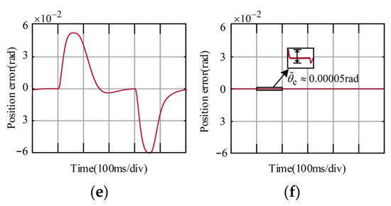
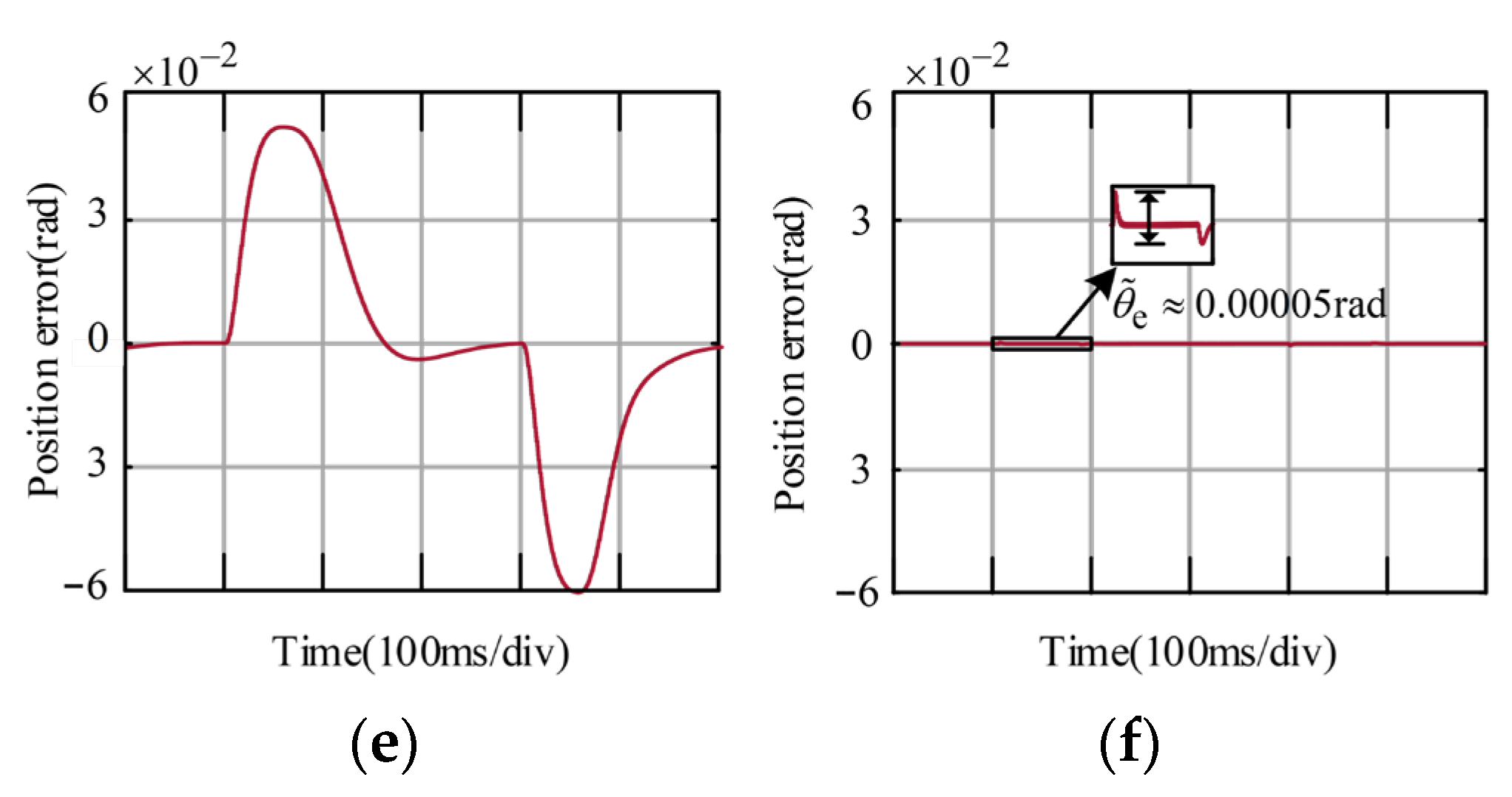
Figure 10. Comparison between the conventional and proposed control strategies under rotating speed references step conditions. (a) Conventional control strategy. (b) Proposed control strategy. (c) Conventional control strategy. (d) Proposed control strategy. (e) Conventional control strategy. (f) Proposed control strategy.

Figure 10c,d present the corresponding current responses. It can be observed that in both strategies, the stator current reaches its peak limit during acceleration and deceleration. However, a noticeably faster current response is achieved under the proposed control strategy.

Figure 10e,f show the results of the position estimation error. It can be observed that the rotor position estimated by the conventional PI-based PLL exhibits a significant error (approximately 0.12 rad) during both speed increase and decrease. Only when the speed is constant does the estimation approach the actual position. In contrast, with the proposed control strategy employing the DDCPLL, the rotor position estimation error remains nearly zero throughout the entire process. Only a slight transient fluctuation (approximately 0.00005 rad) occurs at the instant of speed change, which is far smaller than that of the PI-based PLL.

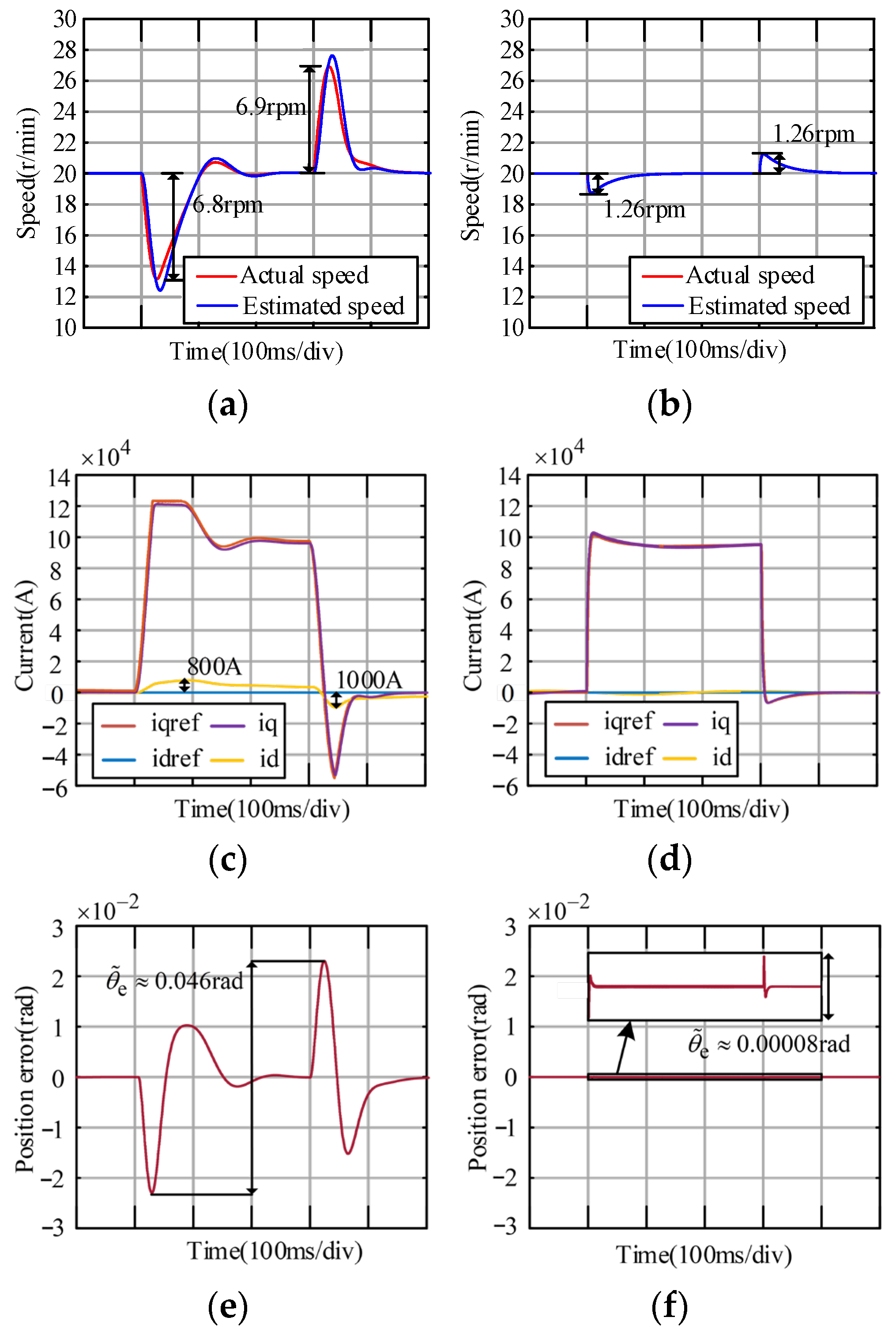
Figure 11 presents a comparison between the conventional and the proposed control strategies under load variation conditions. The scenario involves applying the rated load during steady-state operation and subsequently removing it after stabilization. As shown in Figure 11a, with the conventional strategy, the speed dip and overshoot following load application and removal are 6.8 rpm and 6.9 rpm, respectively, with a settling time of 200 ms. Moreover, a noticeable delay exists in the estimated speed. In contrast, the proposed control strategy results in a significantly reduced speed dip/overshoot of only 1.26 rpm and a settling time of 100 ms, indicating a response approximately 50% faster than the conventional one.

Figure 11. Comparison between the conventional and proposed control strategies under load transients. (a) Conventional control strategy. (b) Proposed control strategy. (c) Conventional control strategy. (d) Proposed control strategy. (e) Conventional control strategy. (f) Proposed control strategy.

Figure 11c,d show the corresponding current responses. It can be observed that at low switching frequencies, the performance of the designed current controller is markedly superior to that of the conventional one. In terms of dynamic response, the designed controller exhibits smaller overshoot and shorter settling time. Regarding decoupling capability, the conventional current controller performs poorly. Figure 11c reveals that after load application, the d-axis current rises due to coupling with the q-axis current, reaching a peak of about 800 A. Upon load removal, the d-axis current drops following the q-axis current, with a peak of 1000 A. Conversely, in the proposed strategy, the d-axis current remains nearly unaffected, validating the effectiveness of the designed current controller.

Figure 11e,f show the simulated position estimation errors during load transients. The results indicate that the position error fluctuation for the PI-based PLL during the load change is 0.046 rad, whereas for the proposed strategy, the error fluctuation for the DDCPLL is only about 0.00008 rad. This demonstrates that the newly designed PLL can accurately and rapidly estimate the actual rotor position even under load variations.

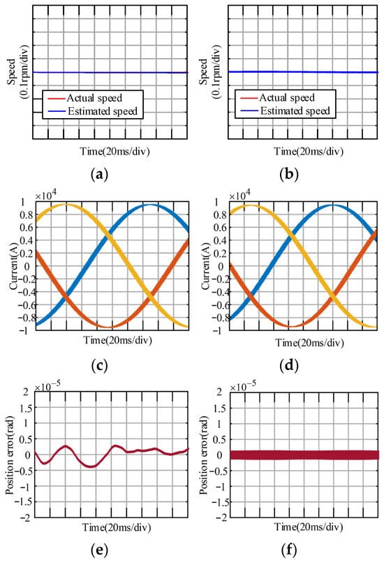
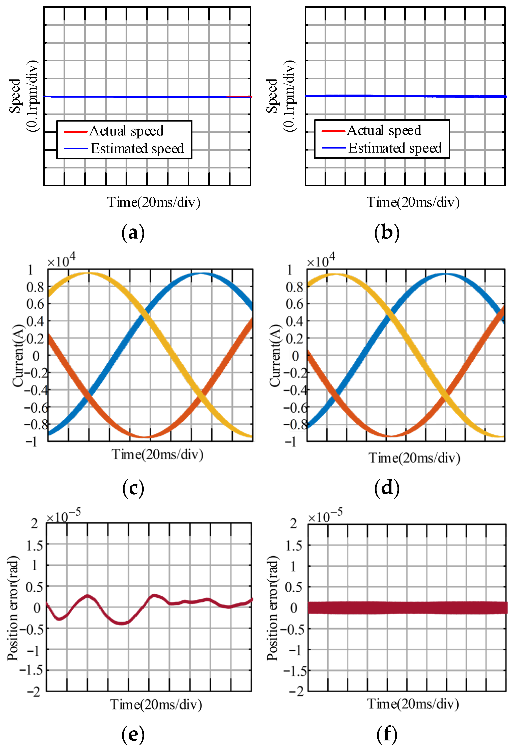
Figure 12 shows the steady-state performance comparison of sensorless control between the conventional strategy and the proposed strategy. At the rated torque, it can be observed that the speed and current performance of both strategies are comparable, with the fluctuation of the position tracking error within the range of ±0.000005 rad. Therefore, it is demonstrated that the proposed control strategy enhances the system’s dynamic response without compromising its steady-state performance.

Figure 12. Steady-Performance Comparison Between Conventional and Proposed Control Strategy. (a) Conventional control strategy. (b) Proposed control strategy. (c) Conventional control strategy. (d) Proposed control strategy. (e) Conventional control strategy. (f) Proposed control strategy.

Based on the above performance verification and analysis, a comparison between the proposed control scheme and sensorless control schemes based on other types of PLLs is summarized in Table 2.

Table 2. Performance comparison of sensorless control methods based on different PLLs.

PLL Type	Reference	Estimation Error (Under Speed Ramp)	Response Speed	Complexity
Conventional PLL	[6,14]	Large	Medium	Simple
FPSPLL	[7,8,9]	Depends on iteration number	Medium to Fast	High
DPLL	[14]	Theoretically zero	Medium	High
APLL	[10]	Relative small	Medium	Medium
DDCPLL	Proposed	Theoretically zero	Medium	Simple

6. Conclusions

To address the two major issues in sensorless control of PMSMs at low switching frequency, namely, the position tracking error of PI-based PLL and the poor performance of the current control loop, this paper proposes a DDCPLL. It resolves the position tracking error of PI-based PLL during speed transients and incorporates a damping factor to balance response speed with smoothness in the estimated speed. Furthermore, a current controller is designed directly in the discrete domain and integrated with the proposed DDCPLL, constructing a complete and accurate discrete-domain model of the position sensorless vector control system, followed by parameter tuning. The proposed DDCPLL achieves fast and accurate estimation of the actual rotor position during speed transients, with significantly higher precision than PI-based PLL. The proposed strategy maintains excellent steady-state performance while achieving markedly superior dynamic response compared to conventional ones. Additionally, the DDCPLL features a simple structure with a single tuning parameter λ, eliminating complex iterations and additional hardware, thus offering low implementation cost. This work provides an effective solution for enhancing the dynamic performance of high-power PMSM sensorless control systems, facilitates the adoption and popularization of sensorless control technology in high-power applications, and contributes to further improving the reliability of high-power PMSM systems.

References

- Jung, S.-Y.; Mi, C.C.; Nam, K. Torque Control of IPMSM in the Field-Weakening Region with Improved DC-Link Voltage Utilization. IEEE Trans. Ind. Electron. 2015, 62, 3380–3387. [Google Scholar] [CrossRef] [Scilit]
- Cai, J.; Gu, Y.; Cheok, A.D.; Yan, Y. A Survey of Phase-Locked Loop Technologies in Sensorless Position Estimation of Permanent Magnet Synchronous Motor Drives. IEEE Trans. Instrum. Meas. 2024, 73, 1–16. [Google Scholar] [CrossRef] [Scilit]
- Wang, Y.; Xu, Y.; Zou, J. Sliding-Mode Sensorless Control of PMSM With Inverter Nonlinearity Compensation. IEEE Trans. Power Electron. 2019, 34, 10206–10220. [Google Scholar] [CrossRef] [Scilit]
- Ortega, R.; Praly, L.; Astolfi, A.; Lee, J.; Nam, K. Estimation of Rotor Position and Speed of Permanent Magnet Synchronous Motors with Guaranteed Stability. IEEE Trans. Control Syst. Technol. 2011, 19, 601–614. [Google Scholar] [CrossRef] [Scilit]
- Bolognani, S.; Calligaro, S.; Petrella, R. Design Issues and Estimation Errors Analysis of Back-EMF-Based Position and Speed Observer for SPM Synchronous Motors. IEEE J. Emerg. Sel. Top. Power Electron. 2014, 2, 159–170. [Google Scholar] [CrossRef] [Scilit]
- Wang, H.; Yang, Y.; Ge, X.; Zuo, Y.; Yue, Y.; Li, S. PLL- and FLL-Based Speed Estimation Schemes for Speed-Sensorless Control of Induction Motor Drives: Review and New Attempts. IEEE Trans. Power Electron. 2022, 37, 3334–3356. [Google Scholar] [CrossRef] [Scilit]
- Abdelrahem, M.; Hackl, C.M.; Kennel, R.; Rodriguez, J. Computationally Efficient Finite-Position-Set-Phase-Locked Loop for Sensorless Control of PMSGs in Wind Turbine Applications. IEEE Trans. Power Electron. 2021, 36, 3007–3016. [Google Scholar] [CrossRef] [Scilit]
- Sun, X.; Cai, F.; Yang, Z.; Tian, X. Finite Position Control of Interior Permanent Magnet Synchronous Motors at Low Speed. IEEE Trans. Power Electron. 2022, 37, 7729–7738. [Google Scholar] [CrossRef] [Scilit]
- Chen, S.; Ding, W.; Hu, R.; Wu, X.; Shi, S. Sensorless Control of PMSM Drives Using Reduced Order Quasi Resonant-Based ESO and Newton–Raphson Method-Based PLL. IEEE Trans. Power Electron. 2023, 38, 229–244. [Google Scholar] [CrossRef] [Scilit]
- Novak, Z.; Novak, M. Adaptive PLL-Based Sensorless Control for Improved Dynamics of High-Speed PMSM. IEEE Trans. Power Electron. 2022, 37, 10154–10165. [Google Scholar] [CrossRef] [Scilit]
- Jiang, F.; Sun, S.; Liu, A.; Xu, Y.; Li, Z.; Liu, X.; Yang, K. Robustness Improvement of Model-Based Sensorless SPMSM Drivers Based on an Adaptive Extended State Observer and an Enhanced Quadrature PLL. IEEE Trans. Power Electron. 2021, 36, 4802–4814. [Google Scholar] [CrossRef] [Scilit]
- Li, Z.; Guo, Y.; Xia, J.; Duan, Y.; Zhang, X. Modified Synchronized SVPWM Strategies to Reduce CMV for Three-Phase VSIs at Low Switching Frequency. IEEE Trans. Ind. Appl. 2020, 56, 5245–5256. [Google Scholar] [CrossRef] [Scilit]
- Chen, Z.; Dawara, A.A.; Zhang, X.; Zhang, H.; Liu, C.; Luo, G. Adaptive Sliding Mode Observer-Based Sensorless Control for SPMSM Employing a Dual-PLL. IEEE Trans. Transp. Electrif. 2022, 8, 1267–1277. [Google Scholar] [CrossRef] [Scilit]
- Wang, H.; Ge, X.; Yue, Y.; Liu, Y.-C. Dual Phase-Locked Loop-Based Speed Estimation Scheme for Sensorless Vector Control of Linear Induction Motor Drives. IEEE Trans. Ind. Electron. 2020, 67, 5900–5912. [Google Scholar] [CrossRef] [Scilit]
- Wang, M.; Buticchi, G.; Li, J.; Gu, C.; Gerada, D.; Degano, M.; Xu, L.; Li, Y.; Zhang, H.; Geradab, C. Decoupled Discrete Current Control for AC Drives at Low Sampling-to-Fundamental Frequency Ratios. IEEE J. Emerg. Sel. Top. Power Electron. 2023, 11, 1358–1369. [Google Scholar] [CrossRef] [Scilit]
- Mon-Nzongo, D.L.; Lin, S.; Ipoum-Ngome, P.G.; Lai, C.; Jin, T.; Rodriguez, J. A Fast-Digital Current Regulator Based on Matched Pole–Zero Discretization for PMSM. IEEE Trans. Transp. Electrif. 2025, 11, 9371–9387. [Google Scholar] [CrossRef] [Scilit]
- Wang, Q.; Yang, S.; Xie, Z.; Zhang, X.; Chang, L. Two-Degree-of-Freedom Discrete-Time Decoupled Current Control of IPMSM With High Parameter Robustness. IEEE J. Emerg. Sel. Top. Power Electron. 2024, 12, 4716–4727. [Google Scholar] [CrossRef] [Scilit]
- Wen, J.; Yuan, X.; Niu, S.; Chan, W.L. A Robust Complex Vector PI Current Controller with Deadbeat Response for PMSM Drives. IEEE Trans. Ind. Electron. 2025, 72, 4671–4681. [Google Scholar] [CrossRef] [Scilit]
- Wu, X.; Kang, J.; Yang, M.; Wu, T.; Huang, S. Robust Deadbeat Predictive Current Control for SPMSM Using Parameter Adaptive Incremental Model. IEEE Trans. Transp. Electrif. 2025, 11, 4609–4618. [Google Scholar] [CrossRef] [Scilit]
- Lu, M.; Wang, X.; Loh, P.C.; Blaabjerg, F.; Dragicevic, T. Graphical Evaluation of Time-Delay Compensation Techniques for Digitally Controlled Converters. IEEE Trans. Power Electron. 2018, 33, 2601–2614. [Google Scholar] [CrossRef] [Scilit]
- Holtz, J.; Quan, J.; Pontt, J.; Rodriguez, J.; Newman, P.; Miranda, H. Design of fast and robust current regulators for high-power drives based on complex state variables. IEEE Trans. Ind. Appl. 2004, 40, 1388–1397. [Google Scholar] [CrossRef] [Scilit]
- Bae, B.-H.; Sul, S.-K. A compensation method for time delay of full-digital synchronous frame current regulator of PWM AC drives. IEEE Trans. Ind. Appl. 2003, 39, 802–810. [Google Scholar] [CrossRef] [Scilit]
- Yim, J.-S.; Sul, S.-K.; Bae, B.-H.; Patel, N.R.; Hiti, S. Modified Current Control Strategies for High-Performance Permanent-Magnet AC Drives with Low Sampling to Operating Frequency Ratio. IEEE Trans. Ind. Appl. 2009, 45, 763–771. [Google Scholar] [CrossRef] [Scilit]
- Zhao, L.; Song, W.; Ruan, Z. Discrete Domain Design Strategy of Complex-Vector Current Controller for Induction Motor at Low Switching Frequency. IEEE Trans. Transp. Electrif. 2023, 9, 404–415. [Google Scholar] [CrossRef] [Scilit]
- Li, Y.; Lin, C.; Xing, J.; Xu, Y. An Improved Discrete-Time Complex Vector Current Regulator for Position Sensorless UhsPMSM Based on Enhanced Active Damping Function. IEEE Trans. Power Electron. 2025, 40, 13822–13834. [Google Scholar] [CrossRef] [Scilit]
Disclaimer/Publisher’s Note: The statements, opinions and data contained in all publications are solely those of the individual author(s) and contributor(s) and not of MDPI and/or the editor(s). MDPI and/or the editor(s) disclaim responsibility for any injury to people or property resulting from any ideas, methods, instructions or products referred to in the content. |
© 2026 by the authors. Licensee MDPI, Basel, Switzerland. This article is an open access article distributed under the terms and conditions of the Creative Commons Attribution (CC BY) license.