The State of Health Prediction of Li-Ion Batteries Based on ISMA-HKELM

Abstract

Accurately predicting the State of Health (SOH) of lithium-ion batteries (LIBs) is essential to ensure their long-term stable and safe operation. This paper proposes a novel model, the ISMA-HKELM, which is an Improved Slime Mould Algorithm (ISMA)-optimized Hybrid Kernel Extreme Learning Machine (HKELM), designed for high-precision SOH estimation. We first selected the equal voltage rise time and equal voltage drop time as indirect health indicators, and their validity was rigorously confirmed through Pearson and Spearman correlation tests. Subsequently, the ISMA was utilized to effectively tune the key parameters of the HKELM model. Experimental results demonstrate that the ISMA-HKELM model exhibits superior prediction performance across multiple public datasets, achieving an average $R^2$ value of more than 0.99. Furthermore, the model shows significantly lower Mean Absolute Error (MAE), Mean Bias Error (MBE), and Root Mean Square Error (RMSE) compared to other control models. These results fully prove the advancement and validity of the ISMA-HKELM model for LIB SOH estimation.

1. Introduction

Lithium-ion batteries (LIBs) have become the dominant electrochemical energy storage technology due to their high energy density, long cycle life, and favorable power capability, enabling broad deployment in consumer electronics, electric vehicles (EVs), and grid-supporting energy systems [1,2]. For EV applications in particular, battery degradation directly impacts practical driving range, charging efficiency, warranty risk, and safety margins, thereby placing stringent requirements on the Battery Management System (BMS) to monitor and prognose battery health throughout the service life [3,4,5]. Among health-related metrics, the State of Health (SOH) is widely adopted as a capacity-based indicator that reflects the usable energy content relative to the nominal (or beginning-of-life) condition. Accurate SOH estimation is therefore essential for condition-aware control, preventive maintenance, and life-cycle management [6].

Existing SOH estimation approaches can be broadly categorized into direct measurement, model-based, and data-driven paradigms. Direct methods rely on laboratory-grade tests to determine capacity, internal resistance, or electrochemical impedance spectroscopy (EIS) signatures [7,8,9], which are accurate but often costly and time-consuming for routine online use [10]. Model-based methods construct electrochemical or equivalent-circuit representations and infer latent states via observers or filtering strategies. These approaches are attractive for interpretability, yet they typically require careful parameterization [11] and can face robustness challenges under changing operating conditions, cell-to-cell variability, and non-stationary aging mechanisms [12,13,14]. Data-driven approaches analyze empirical data to extract health indicatorsand estimate SOH by modeling the nonlinear correlations between these indicators and aging variables [15]. This paradigm is favored as it circumvents the need for intricate electrochemical process analysis, providing a straightforward avenue for SOH prediction. Recent advancements in this domain encompass architectures leveraging nonlinear autoregressive networks [16], algorithms such as the Extreme Learning Machine (ELM) [17,18,19], and optimization strategies like NSGA-II [20] and the Sparrow Search Algorithm (SSA) [21]. Additionally, models integrating incremental capacity analysis with neural networks have been explored [22,23]. More recently, cutting-edge techniques involving time-series convolutional networks [24,25], physics-informed lightweight Transformers (PLT-GRU) [26,27], frequency-domain enhanced frameworks [28], and transfer learning coupled with graph neural networks (GNNs) [29] have been introduced. In contrast, data-driven methods learn a mapping from measurable signals (or engineered health indicators) to SOH [30,31], aiming to capture complex nonlinear aging effects without explicitly modeling the underlying electrochemistry [6,15].

In the last few years, data-driven SOH estimation has progressed along two complementary directions: feature-driven learning with physically meaningful health indicators, and representation learning that reduces manual feature engineering. In feature-driven learning, researchers have designed health indicators from voltage/current trajectories, differential/incremental analysis, impedance, and thermal responses, and then applied machine learning regressors or lightweight neural networks for SOH mapping [9,17]. Such strategies preserve interpretability and often suit low-compute BMS deployment, but their reliability can depend strongly on signal quality and the availability of consistent full-cycle data [32]. In representation learning, deep architectures such as recurrent networks, convolutional time-series models, and hybrid CNN–RNN designs [16,24,25] are trained to extract latent aging features directly from raw or minimally processed sequences [33]. Recently, attention-based models and Transformer variants have been increasingly explored for capturing long-range temporal dependencies and complex sequence patterns, including multi-step prediction via optimized Transformer structures and hybrid convolutional/attention blocks [26,27]. Multi-feature attention collaboration and end–cloud Transformer frameworks, as well as Transformer models with data augmentation, have further advanced SOH estimation performance [34,35,36]. In parallel, cross-domain learning has been emphasized to mitigate distribution shifts across chemistries, manufacturers, and operating conditions, for example via transfer learning and graph-based modeling [29,37]. More broadly, large-scale learning paradigms have emerged, including domain adaptation frameworks that reduce the need for extensive target-labeled degradation experiments [38].

Despite these advances, several obstacles remain for reliable SOH estimation in real-world BMS settings. First, practical battery operation often lacks complete and standardized charge/discharge cycles, which can compromise methods that assume full-cycle features or fixed voltage windows. Studies have therefore investigated partial-charge (or partial-cycle) learning, but performance can still be sensitive to missing segments and condition changes [38]. Second, strong variability in ambient temperature, load profiles, and sensor noise creates non-stationary data distributions that degrade generalization if models are trained and validated under overly idealized experimental splits. Third, while high-capacity deep networks can be accurate, they may be difficult to deploy due to training cost, tuning burden, and inference constraints. To address these issues, recent works have explored lightweight Transformer designs and hybrid schemes; at the same time, emerging foundation-model ideas (e.g., generative pre-trained Transformers) suggest new directions for early-stage degradation prediction, albeit with substantial data and computation requirements [39].

Kernel-based learning offers a compelling middle ground between purely shallow regressors and large deep networks. In particular, the Extreme Learning Machine (ELM) family is known for efficient learning dynamics and favorable generalization in many regression settings [40]. When combined with kernelization, ELM can model nonlinear relationships more flexibly while retaining a relatively simple computational structure. However, kernel methods are highly sensitive to kernel choice and hyperparameter settings, and a single kernel may not simultaneously capture both local nonlinearities and global trends across the full aging trajectory. Hybrid kernel strategies, which integrate complementary kernels such as the radial basis function (RBF) and polynomial kernels, can enhance expressivity and robustness, but they amplify the hyperparameter optimization challenge due to higher-dimensional search spaces and potential parameter coupling [41,42].

In this context, this work develops an ISMA-optimized Hybrid Kernel Extreme Learning Machine (ISMA-HKELM) framework for accurate and efficient SOH estimation across diverse public datasets. The proposed method is designed around two practical considerations for BMS deployment: (i) extracting indirect yet interpretable health indicators from standard cycling signals, and (ii) employing a computationally light predictor whose performance can be systematically improved via robust hyperparameter tuning. Specifically, we select equal voltage rise time and equal voltage drop time as indirect health indicators, and statistically validate their strong association with SOH via Pearson and Spearman correlation analyses. Then, a hybrid kernel ELM is employed to capture nonlinear aging behavior with improved flexibility compared to single-kernel formulations. To address hyperparameter sensitivity and avoid suboptimal manual tuning, we introduce an Improved Slime Mould Algorithm (ISMA) to optimize the HKELM hyperparameters in a gradient-free manner, targeting stable performance under realistic validation protocols.

The main contributions of this study are summarized as follows:

• Interpretable indicator construction and validation: Indirect health indicators derived from equal-voltage time intervals are extracted from charging/discharging data and validated using both Pearson and Spearman correlation analyses, providing a transparent link between measurable signals and SOH.
• Efficient nonlinear modeling via hybrid kernel learning: A hybrid kernel ELM architecture is adopted to better balance local nonlinear approximation (RBF) and global trend representation (polynomial), improving the capability to model long-term degradation trajectories with low inference cost.
• Robust hyperparameter optimization with ISMA: An improved slime mould optimization strategy is used to automatically tune key HKELM hyperparameters, alleviating kernel sensitivity and enhancing generalization without relying on exhaustive manual search.
• Cross-dataset verification under more rigorous validation: The proposed framework is evaluated on representative public datasets (NASA and CALCE) to demonstrate accuracy and generalization potential, with validation designed to better reflect degradation prediction settings than naive random splits.

The remainder of the paper is organized as follows: Section 2 introduces the datasets and health indicator extraction procedure. Section 3 describes the ISMA-HKELM methodology. Section 4 reports experimental results and analysis. Finally, Section 5 concludes the paper.

2. Data Analysis

2.1. Introduction to LIBs Dataset

This study utilizes two prominent lithium-ion battery (LIB) datasets, namely NASA PCoE and CALCE, to forecast the State of Health (SOH).

NASA LIBs Dataset: The battery aging dataset released by the NASA Prognostics Center of Excellence (PCoE) [43], encompassing cells B0005, B006, B007, and B0018, is a cornerstone for degradation modeling and predictive analysis. This repository offers detailed time-series data for charge–discharge events, logging essential parameters including voltage, current, and temporal information.

CALCE LIBs Dataset: Data sourced from the University of Maryland’s Center for Advanced Life Cycle Engineering (CALCE) [44] is widely utilized as a reference for assessing battery degradation and longevity. Specifically, this work investigates cells CS2_36 and CS2_37, which underwent cycling experiments within a temperature window of 20 °C to 25 °C.

2.2. Indirect Health Factors

The SOH of LIBs is a key factor in measuring their aging and health level, which can be defined by Equation (1).

$$\mathrm{SOH}={\displaystyle \frac{Q_{\mathrm{new}}}{Q_{\max }}}$$

(1)

$Q_{\max }$ signifies the nominal capacity of LIBs. In contrast, $Q_{\mathrm{new}}$ represents the per-cycle discharge capacity, determined by calculating the time integral of the current during the discharge phase up to the voltage cutoff point.

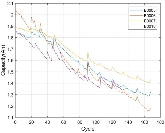
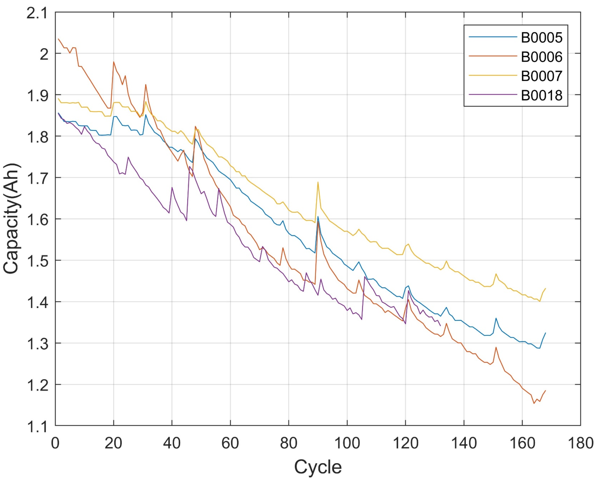
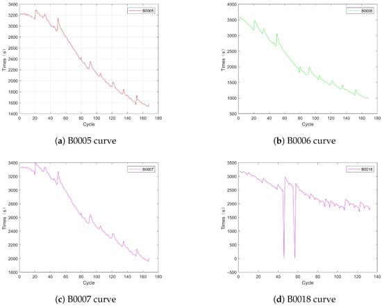
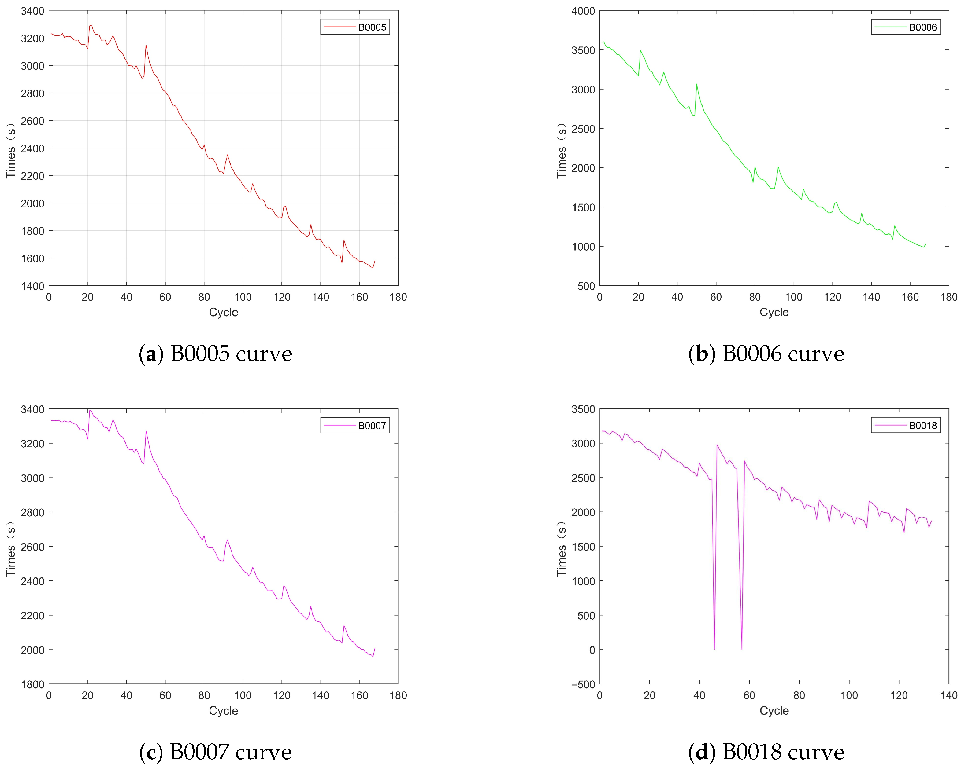
The capacity decay curves of four LIBs are presented in Figure 1. While capacity fade and internal resistance growth are widely accepted as the primary Direct Health Indicators (DHIs) for batteries, their measurement necessitates the use of expensive instrumentation and is inherently time-consuming, posing significant challenges for online data collection. Furthermore, discharge data often exhibits inherent instability, where environmental interference can lead to inaccurate measurements. Crucially, in practical applications, LIBs are rarely subjected to a full discharge cycle. Therefore, extracting various indirect health indicators (IHIs) by analyzing the charging or discharging processes of LIBs is advantageous. This approach reflects the battery health status from multiple perspectives, allowing for a more comprehensive capture of the aging-related information of LIBs.

Figure 1. The capacity decay curves.

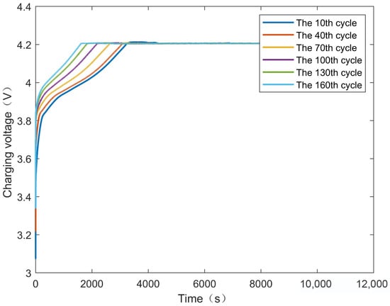
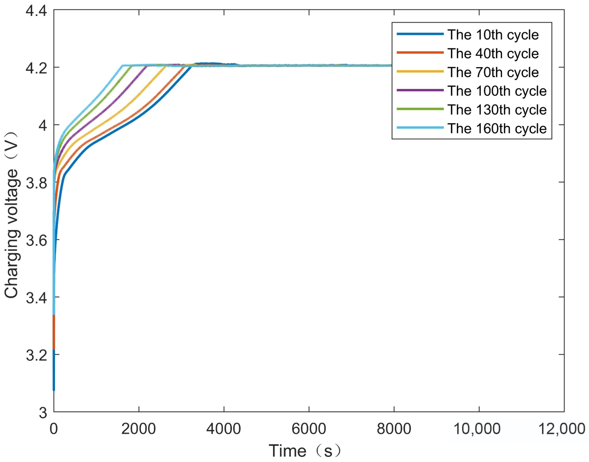
In the constant current (CC) phase, lithium-ion batteries (LIBs) receive a steady current until the terminal voltage hits the 4.2 V upper limit. Figure 2 displays the voltage evolution for cell B0005, highlighting specific profiles at cycles 10, 40, 70, 100, 130, and 160. This same logging procedure was applied across all battery models to capture voltage dynamics for every full charge cycle.

Figure 2. B0005 voltage dynamic change curve.

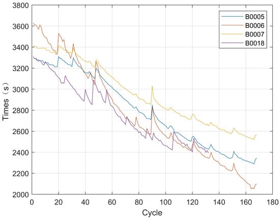
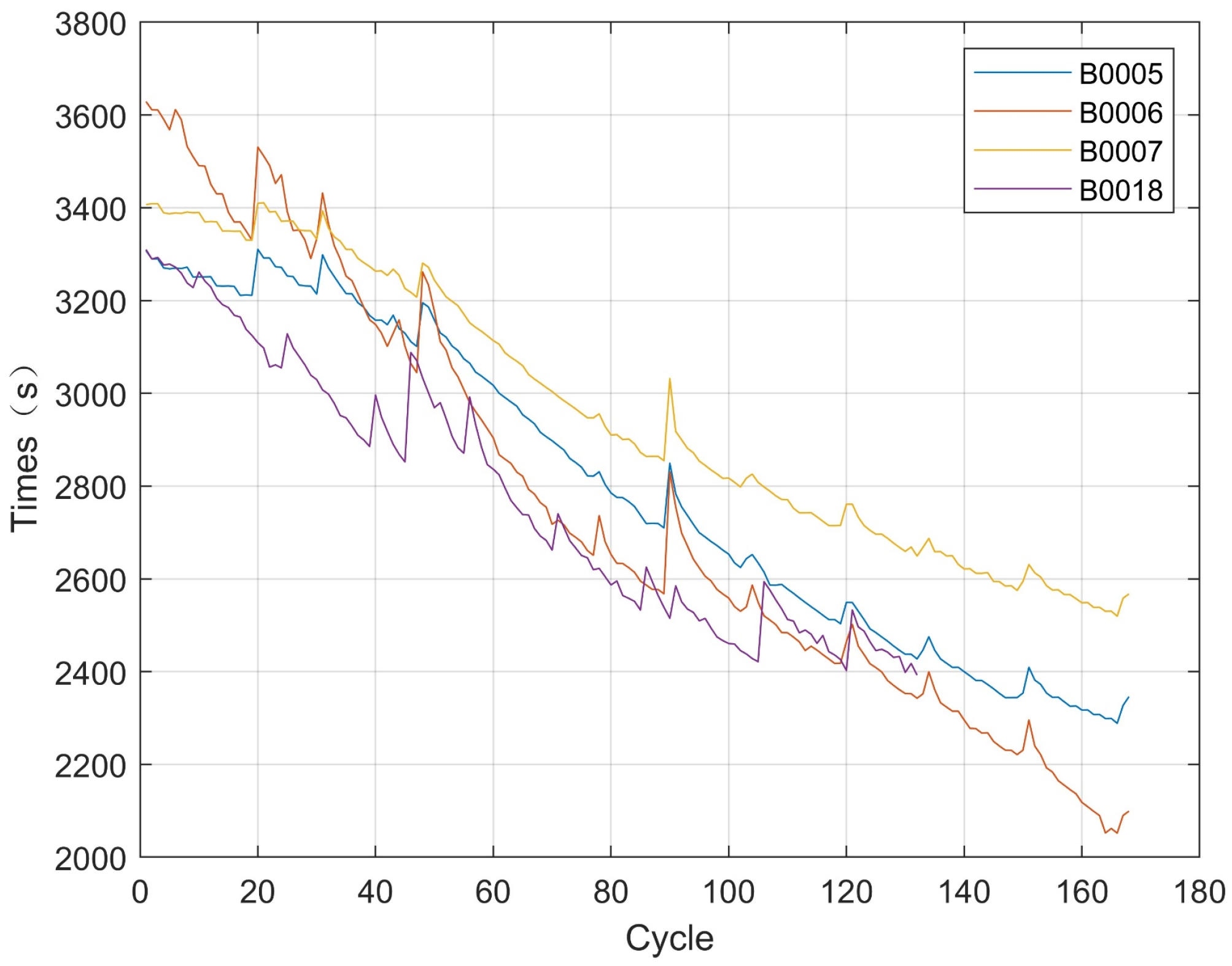
During charging, the duration it takes for the terminal voltage to increase from 3.0 V to 4.2 V is defined as the equal voltage rise time. Because this duration lengthens as the battery degrades, it serves as a reliable indicator of health status. Figure 3 plots the changes in this rise time for batteries B0005 through B0018 against the cycle count. For each charging sequence, we calculate the time elapsed between 3.0 V and 4.2 V, designating this metric as Health Factor 1 (HF1).

Figure 3. Battery equal voltage rise time curve.

Likewise, we define the equal voltage drop time as the duration it takes for the potential to decrease from 4.2 V to 2.8 V while discharging. Figure 4 depicts the trend of this drop time for the B0005–B0018 series over their operational life. By processing data from each discharge event, we extract the time interval for the 4.2 V to 2.8 V transition, labeling it as Health Factor 2 (HF2).

Figure 4. Battery equal voltage drop time curve.

From an electrochemical perspective, the equal-voltage rise time (HF1) during CC charging reflects the dynamic polarization response of the cell. As aging progresses, internal resistance increases and charge-transfer kinetics slow down due to SEI thickening and loss of active lithium, leading to a longer time required to traverse the same voltage window. Similarly, the equal-voltage drop time (HF2) during discharge is related to usable capacity and overpotential behavior under load. Capacity loss and increased ohmic/polarization drops accelerate voltage decay, making the discharge voltage window traverse faster. Therefore, HF1 and HF2 are physically linked to degradation mechanisms such as resistance growth, SEI formation, and lithium inventory loss, providing interpretable proxies for SOH.

The identical data processing strategy was employed for the CALCE datasets CS2_36 and CS2_37. We extract HF1 as the charging interval spanning the voltage rise from 3.0 V to 4.2 V. Similarly, HF2 is identified as the discharge period corresponding to a voltage drop from 4.2 V down to 2.8 V. The selected range for HF1 (3.0 V–4.2 V) is pivotal because it covers the primary plateau of the constant-current charge, a region where significant electrochemical variations linked to aging take place. Regarding HF2, the lower boundary was intentionally set to 2.8 V to better detect degradation signs in the low-voltage zone. Although a broad voltage window improves feature distinction in full-cycle tests, it is recognized that adaptive or narrower windows might be more suitable for partial-state-of-charge (PSOC) scenarios.

We utilized Pearson and Spearman correlation analyses as our main statistical methods. The Pearson coefficient is chiefly used to quantify the linear dependence between continuous variables. On the other hand, the Spearman rank coefficient evaluates the strength of monotonic relationships, making it highly effective for continuous, discrete, or ordinal data types. The formulas governing these analyses are detailed in Equations (2) and (3).

$$\mathrm{Pearson}={\displaystyle \frac{{\sum }_{i=1}^n(x_i-\overline{x})(y_i-\overline{y})}{\sqrt{{\sum }_{i=1}^n{(x_i-\overline{x})}^2{\sum }_{i=1}^n{(y_i-\overline{y})}^2}}}$$

(2)

where $\overline{x}$ and $\overline{y}$ are the average values of x and y.

$$\mathrm{Spearman}=1-{\displaystyle \frac{6\sum d_i^2}{n(n^2-1)}}$$

(3)

where $d_i$ is the difference between the ranks of the i-th observation for x and y.

Based on the aforementioned data, we extracted the indirect health factors of two lithium-ion batteries and calculated their correlation coefficients with the SOH. The results are presented in Table 1. All the calculated correlation coefficients exceed 0.9, indicating a significant correlation between the extracted indirect health factors and SOH. This provides a robust foundation for predicting their future trends.

Table 1. HF and SOH correlation coefficients.

No.	Spearman Coefficient		Pearson Coefficient
	HF1	HF2	HF1	HF2
B0005	0.9889	0.9941	0.9956	0.9977
B0006	0.9937	0.9998	0.9920	0.9999
B0007	0.9921	0.9991	0.9957	0.9997
B0018	0.9676	0.9996	0.9838	0.9998
CS2_36	0.9965	0.9997	0.9971	0.9997
CS2_37	0.9943	0.9997	0.9963	0.9998

Regarding robustness under operating variations, the selected voltage windows (3.0–4.2 V for charge and 4.2–2.8 V for discharge) lie in the main CC plateau where the voltage response is relatively stable and repeatable, which reduces sensitivity to short-term noise. Nevertheless, temperature and C-rate shifts can still influence polarization and thus the absolute timing values. In practice, consistent operating protocols or normalization strategies are recommended to maintain comparability. For partial-state-of-charge scenarios, narrower adaptive windows can be considered, and this represents a limitation and a potential extension of the present study.

3. Methods

3.1. The Improved Slime Mould Algorithm

The Slime Mould Algorithm (SMA) [45] is a novel stochastic optimization algorithm whose inspiration is drawn from the oscillatory patterns observed in slime moulds within their natural habitat.

We propose an improved Slime Mould Algorithm (ISMA) in this paper. Mathematically, unlike the original SMA which employs a linear decay parameter a (decreasing linearly from 1 to 0), ISMA introduces a nonlinear decreasing strategy (Equation (5)) to better balance exploration and exploitation phases. The use of the inverse hyperbolic tangent function allows the parameter a to decrease slowly in the early stages (facilitating global exploration) and rapidly in the later stages (enhancing local exploitation). Furthermore, the adaptive opposition-based learning strategy allows the algorithm to escape local optima by generating candidate solutions in the opposite direction of the current search space. These strategies collectively refine the SMA model, providing a theoretical guarantee for avoiding premature convergence and accelerating the search for the global optimum.

Elite Reverse Initialization Population

The elite opposition-based population initialization is a specialized technique used in optimization algorithms to broaden population diversity and boost search performance. This elite opposition-based learning approach works by creating new candidate solutions via an opposition mechanism based on the current best individual. Its main goal is to exploit the traits of elite agents and map them inversely to other agents, thereby establishing a more diverse starting population.

The starting population $X_0=\mathrm{initialization}(N,\dim ,\mathrm{ub},\mathrm{lb})$ is formed using standard protocols, where N represents the total count of agents, dim indicates the dimensionality of the search space, and ub and lb specify the upper and lower constraints for each dimension. Following the assignment of initial positions for the search agents, the opposition-based population is computed as per Equation (4).

$$X_1(i,j)=\left(u_{\mathrm{b}}{+|}_{\mathrm{b}}\right)-X_0(i,j)$$

(4)

The initial population $X_0$ and the reverse population $X_1$ are combined to form an overall population X containing all individuals, thereby increasing the diversity and quality of the population.

Nonlinear Decreasing Strategy

The algorithm adopts a nonlinear decreasing strategy combined with dynamic parameters, updating the fitness judgment to update the population position. Using Equations (5) and (6), dynamic updates of variables a and b are calculated by controlling their gradual reduction, prompting the algorithm’s search range to converge progressively with iterations. In this context, iter signifies the current iteration step, while Max_iter corresponds to the predefined maximum number of iterations for the algorithm.

$$\mathrm{a}={\tanh }^{-1}\left(1-{\displaystyle \frac{\mathrm{iter}}{\text{Max\_iter}}}-ϵ\right),ϵ\to 0^{+}$$

(5)

In Equation (5), ${\tanh }^{-1}$ denotes the inverse hyperbolic tangent function (arctanh). Mathematically, $\mathrm{arctanh}\left(x\right)$ is undefined when $x=1$. To prevent the singular point at the initial iteration ($\mathrm{iter}=0$) and ensure numerical stability, a small positive constant $ϵ$ is introduced. In our implementation, $ϵ$ is set to a machine-precision value (e.g., ${10}^{-16}$), which is sufficient to ensure that the argument of ${\tanh }^{-1}$ is strictly less than 1, thereby guaranteeing the boundedness of parameter a.

$$b=1·{\left(1-{\displaystyle \frac{\mathrm{iter}}{\text{Max\_iter}}}\right)}^{{\displaystyle \frac{\mathrm{iter}}{\text{Max\_iter}}}}$$

(6)

Adaptive Opposition-Based Learning

The adaptive opposition-based learning (AOBL) method [46] is a popular approach in algorithmic optimization. During its application, all solutions within the population are first ranked according to their respective fitness values. The fitness value serves as an indicator of a solution’s quality or performance, where a higher value signifies a better solution. Following this sorting process, the population is bifurcated into two distinct parts: the first $N/2$ solutions, which possess high fitness values, are designated as superior solutions, and their corresponding weights are derived using Equation (7). Conversely, the latter $N/2$ solutions, characterized by relatively low fitness values, are considered inferior solutions, with their weights subsequently obtained using Equation (8).

$$\mathrm{weight}\left(\mathrm{SlimeOrder}\left(i\right),j\right)=1+\mathrm{rand}·{log}_{10}\left({\displaystyle \frac{\mathrm{bestFitness}-\mathrm{SlimeOrder}\left(i\right)}{s}}+1\right)$$

(7)

$$\mathrm{weight}\left(\mathrm{SlimeOrder}\left(i\right),j\right)=1-\mathrm{rand}·{log}_{10}\left({\displaystyle \frac{\mathrm{bestFitness}-\mathrm{SlimeOrder}\left(i\right)}{s}}+1\right)$$

(8)

In this study, we define $weight\left(SlimeOrder\left(i\right),j\right)$ as the fitness weighted value of the i-th slime mould population ranked in ascending order on the j-th dimension, where $rand$ denotes a random value generated in the range of 0 to 1. $bestFitness$ and $worstFitness$ represent the best- and worst-performing fitness values of the population, respectively. The maximum difference in the fitness values of the population, S, is calculated by Equation (9), where $ϵ$ is a minimal positive value that prevents S from being zero.

$$S=\mathrm{bestFitness}-\mathrm{worstFitness}+ϵ$$

(9)

Two random numbers are generated, and when $r_1$ is less than a preset threshold $\delta$, the position of population $X(i,j)$ is obtained by randomly re-initializing the search using Equation (10).

$$X(i,j)=(\mathrm{ub}-\mathrm{lb})\times \mathrm{rand}+\mathrm{lb}$$

(10)

When the preset threshold $\delta$ is satisfied, the fitness update probability and random perturbation vector are automatically generated to determine the population location. The hyperbolic tangent function of the fitness difference is computed by Equation (11).

$$p=tanh\left(\left|\mathrm{oldfitness}\left(i\right)-\mathrm{Destination}\mathrm{fitness}\right|\right)$$

(11)

where $oldfitness\left(i\right)$ denotes the fitness value of each i-th individual in the previous iteration, and Destination_fitness denotes the target fitness value.

$v_a\sim U(-a,a)$, i.e., in the range $[-a,a]$, $v_a$ is a randomly drawn perturbation value from the uniform distribution $U(-a,a)$.

$v_b\sim U(-b,b)$, i.e., in the range $[-b,b]$, $v_b$ is a randomly drawn perturbation value from the uniform distribution $U(-b,b)$.

If $r_2<p$, use Equation (12) to update the position of individuals in the j-th dimension of the population.

If $r_2>p$, use Equation (13) to update the population’s individual positions by perturbing $v_b\left(j\right)$.

$$X(i,j)=\mathrm{bestPositions}\left(j\right)+v_a\left(j\right)·\left(\mathrm{weight}(i,j)·\mathrm{bestPositions}\left(j\right)-X(A,j)\right)$$

(12)

$$X(i,j)=v_{\mathrm{b}}\left(j\right)·X(i,j)$$

(13)

3.2. The HKELM Model

The modified Hybrid Kernel Extreme Learning Machine (HKELM) [47] model represents an innovation derived from the traditional Extreme Learning Machine (ELM) [40]. This model strategically incorporates the advantages of multiple kernel functions to enhance its learning efficiency and broaden its applicability.

HKELM employs a strategy that blends a Radial Basis Function (RBF) kernel [48] with a Polynomial (Poly) kernel [49], thereby significantly improving the fitting performance of the overall model. This hybrid kernel approach optimizes the resolution of the data’s inherent nonlinear properties by projecting the input data into a high-dimensional feature space under the action of the combined kernel. Within this feature space, the data is fitted using linear regression methods to determine the output weight values required for prediction. Utilizing these obtained weight values, the model is then capable of making robust predictions for new, unseen datasets.

Specifically, we have utilized the RBF kernel function, which is defined as shown in Equation (14). Similarly, the polynomial kernel function is also employed, with its definition provided in Equation (15).

$$K_{\mathrm{RBF}}(x,y)=exp\left(-{\displaystyle \frac{{\parallel x-y\parallel }^2}{2{\sigma }^2}}\right)$$

(14)

$$K_{\mathrm{Poly}}(x,y)={(x·y+r)}^d$$

(15)

Here, $\sigma$ represents the variance of the RBF kernel, while r and d denote the bias and degree of the polynomial kernel, respectively.

The hybrid kernel extreme learning machine process is as follows:

Load the dataset, and set $X_{train}$ as the training data, which has one input for each row; $X_{test}$ is the test data, which has one input for each row. Introduce the RBF and polynomial kernel function, set $\sigma$ (the variance parameter of the RBF kernel), the bias parameter r of the polynomial kernel, and the order d of the polynomial kernel. The kernel matrix ${\Omega }_t\in {\mathbb{R}}^{N_{train}\times N_{test}}$ is constructed to map the input features into a high-dimensional space, capturing the nonlinear relationships. It is calculated as a weighted sum of RBF and Polynomial kernels (Equation (16)):

To reduce the risk of overfitting, the regularization term is introduced to calculate the output weights using Equation (17), where $T_{\mathrm{train}}^T$ is the transpose of the target matrix of the training data, c is the regularization parameter, and I is the unit matrix, which has the same size as the kernel matrix ${\Omega }_t$.

Map the test data to the same feature space as the training data, and then use the output weights learned during the training phase to compute the predictions with Equation (18).

$${\Omega }_{\mathrm{t}}=\alpha ·K_{\mathrm{RBF}}(X_{\mathrm{train}},X_{\mathrm{test}})+(1-\alpha )·K_{\mathrm{Poly}}(X_{\mathrm{train}},X_{\mathrm{test}})$$

(16)

$$W_{\mathrm{output}}={\left({\Omega }_{\mathrm{t}}+{\displaystyle \frac{1}{c}}\mathrm{I}\right)}^{-1}{\mathrm{T}}_{\mathrm{train}}^{\mathrm{T}}$$

(17)

$$\text{Test\_out}={\left({\Omega }_{\mathrm{test}}^T·W_{\mathrm{output}}\right)}^T$$

(18)

3.3. The ISMA-HKELM Model

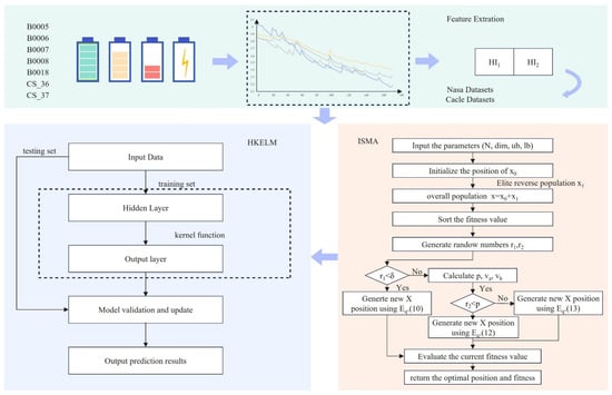
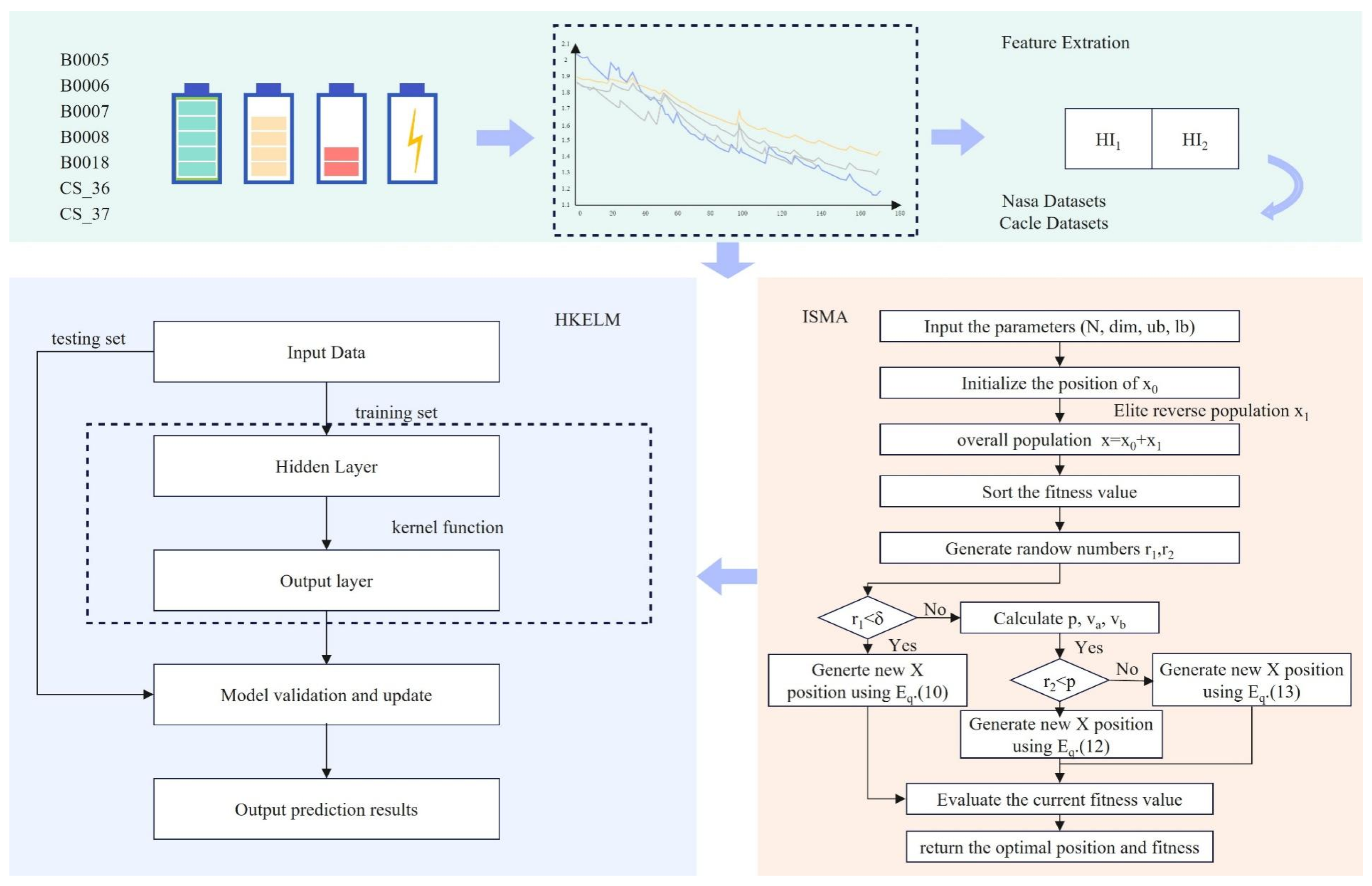
The ISMA-HKELM framework was developed by utilizing the previously defined HF1 and HF2 (see Section 2) as input features to estimate the SOH of lithium-ion batteries. To boost forecasting precision, ISMA is utilized to optimally tune the regularization coefficient and kernel settings specific to the HKELM structure. Figure 5 depicts the schematic of the proposed model, which proceeds through the following key stages:

Figure 5. The architecture of the ISMA-HKELM model.

Data Preprocessing: Following a comprehensive examination of the NASA and CALCE repositories, we extract and process the health factors (HF1, HF2) alongside the actual SOH values, calculated as the quotient of current discharge capacity to nominal capacity. Subsequently, the dataset undergoes a random split: $60\%$ of the cycle data is designated for model training, while the remaining $40\%$ is set aside strictly for performance assessment.

ISMA Parameter Setup: The ISMA optimizer is configured with a population count of $N=50$ and a termination criterion of $\text{Max\_iter}=1000$. Every agent within the population represents a potential vector of HKELM hyperparameters, comprising:

• The regularization parameter c;
• The weighting factor $\alpha$ that blends RBF and polynomial kernels;
• The width parameter $\sigma$ for the RBF kernel;
• The polynomial kernel’s bias r and power d.

HKELM Training and Fitness Evaluation: For every agent within the ISMA population, its specific hyperparameters serve to build the hybrid kernel matrix ${\Omega }_t$ based on the training data, following Equation (16). Subsequently, the Moore–Penrose pseudoinverse is applied to calculate $\mathbf{W}$_output, as detailed in Equation (17). Finally, the SOH predictions for the training instances are derived through Equation (18).

Crucially, the fitness score for every candidate is determined exclusively by calculating the mean squared error (MSE) comparing the forecasted and ground-truth SOH values across the training data:

$$\mathrm{Fitness}={\displaystyle \frac{1}{N_{\mathrm{train}}}}\sum _{i=1}^{N_{\mathrm{train}}}{\left(y_i-{\widehat{y}}_i\right)}^2,$$

(19)

where $y_i$ and ${\widehat{y}}_i$ denote the true and predicted SOH values, respectively. The test set is never accessed during the optimization process, ensuring an unbiased assessment of generalization performance.

Parameter Optimization and Final Prediction: The ISMA iteratively updates the population by mimicking the oscillatory foraging behavior of slime moulds, guided by the fitness values, with the goal of minimizing prediction error on the training data while maintaining model stability through regularization. Once the optimal hyperparameter set is identified, the HKELM model is retrained on the full training set and then applied to the held-out test set to produce the final SOH predictions.

This design ensures that the ISMA-HKELM framework adheres to standard machine learning protocols: hyperparameter tuning is performed without any information leakage from the test data, and model performance is evaluated under realistic deployment conditions.

4. Experimental Results

4.1. Evaluation Indicators

To comprehensively evaluate the proposed model’s efficacy, we employ the mean absolute error (MAE), mean bias error (MBE), root mean square error (RMSE), and the coefficient of determination ($R^2$) as validation metrics, with the computed results detailed subsequently.

$$MAE=max|f\left(x_i\right)-y_i|$$

(20)

$$RMSE=\sqrt{{\displaystyle \frac{1}{n}}\sum _{i=1}^n{\left(f\left(x_i\right)-y_i\right)}^2}$$

(21)

$$MBE={\displaystyle \frac{1}{n}}\sum _{i=1}^n\left(y_i-{\overline{y}}_i\right)$$

(22)

$$R^2=1-{\displaystyle \frac{{\sum }_{i=1}^n{\left(f\left(x_i\right)-y_i\right)}^2}{{\sum }_{i=1}^n{\left(f\left(x_i\right)-{\overline{y}}_i\right)}^2}}$$

(23)

In the above equations, n denotes the number of samples, $f\left(x_i\right)$ represents the SOH estimated by the model, $y_i$ is the actual SOH value, and ${\overline{y}}_i$ refers to the average of the actual SOH values.

The smaller the MAE and RMSE values, the higher the prediction accuracy of the model. The closer the $R^2$ value is to 1, the better the model fits the data. MBE is used to measure the average deviation of prediction errors; the closer the MBE value is to 0, the stronger the prediction ability of the model.

4.2. ISMA Performance Test

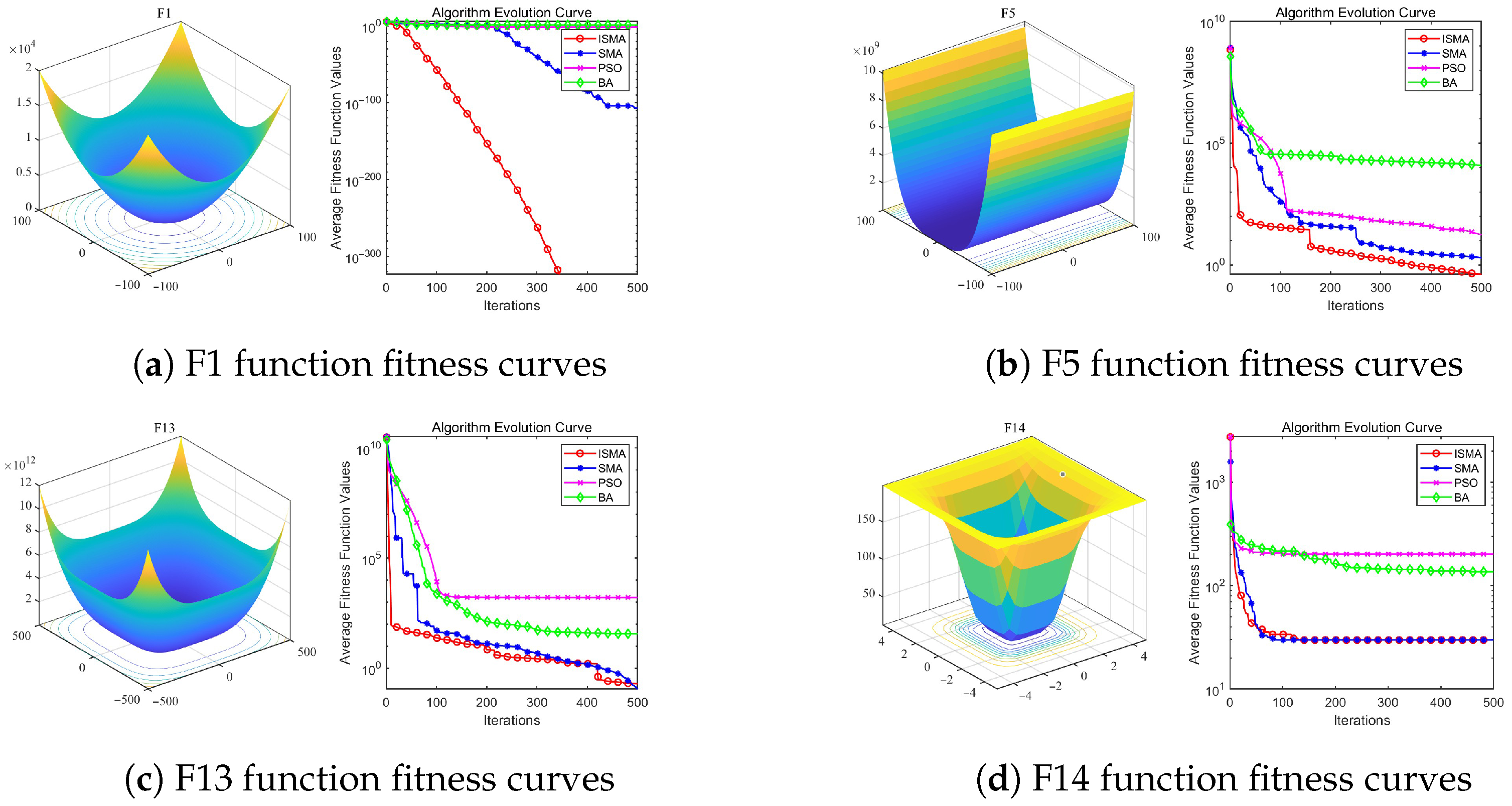
In this section, we select a variety of standard benchmark problems to validate the enhancements of ISMA. The unimodal functions (F1–F7) are utilized to test the solver’s proficiency in locating the global optimum. Meanwhile, the multimodal functions (F8–F13) and fixed-dimension multimodal problems (F14, F16, F18) are employed to gauge the algorithm’s global exploration capability (avoiding local optima), as well as its convergence rate and stability.

To evaluate the impact of these improvements, ISMA is benchmarked against SMA, Particle Swarm Optimization (PSO) [50], and the Bat Algorithm (BA) [51]. Table 2 summarizes the performance of ISMA, SMA, PSO, and BA on these test functions: reporting the mean and standard deviation in sequence. For every algorithm, the first row indicates the average objective value, with the top-performing results marked in bold.

Table 2. Benchmark function results for ISMA, SMA, PSO and BA method tests.

F	Metrics	ISMA	SMA	PSO	BA
F1	Mean	$\mathbf{0}$	$-6.6814\times {10}^{-75}$	0.0020	0.5923
	Variance	$\mathbf{0}$	$2.1129\times {10}^{-74}$	0.0056	0.1548
F2	Mean	$\mathbf{0}$	$-1.5461\times {10}^{-65}$	$7.0126\times {10}^{-23}$	0.1108
	Variance	$\mathbf{0}$	$2.678\times {10}^{-65}$	$1.0013\times {10}^{-22}$	0.0331
F3	Mean	$\mathbf{0}$	$-1.4309\times {10}^{-72}$	$1.2858\times {10}^{-42}$	0.0057
	Variance	$\mathbf{0}$	$2.4767\times {10}^{-72}$	$5.5972\times {10}^{-42}$	0.0037
F4	Mean	$\mathbf{0}$	$-6.5745\times {10}^{-109}$	$4.801\times {10}^{-25}$	0.0146
	Variance	$\mathbf{0}$	$9.2512\times {10}^{-109}$	$6.6134\times {10}^{-25}$	0.0057
F5	Mean	$\mathbf{0}.\mathbf{0393}$	0.6827	0.42271	1146.1842
	Variance	$\mathbf{0}.\mathbf{1452}$	0.1734	1.4782	2423.9788
F6	Mean	$\mathbf{6}.\mathbf{615}\times {\mathbf{10}}^{-\mathbf{5}}$	$-0.5112$	2.6053	7.5395
	Variance	$\mathbf{3}.\mathbf{7618}\times {\mathbf{10}}^{-\mathbf{5}}$	$8.0783\times {10}^{-4}$	1.029	0.9838
F7	Mean	$\mathbf{8}.\mathbf{429}\times {\mathbf{10}}^{-\mathbf{5}}$	$-0.0215$	0.0027	0.0049
	Variance	$\mathbf{8}.\mathbf{6775}\times {\mathbf{10}}^{-\mathbf{5}}$	0.0303	0.00268	0.0038
F8	Mean	$-7.8906$	5.2391	$-7.8906$	$-\mathbf{5}.\mathbf{7761}\times {\mathbf{10}}^{\mathbf{90}}$
	Variance	$1.787\times {10}^{-8}$	0.0002	$\mathbf{5}.\mathbf{1075}\times {\mathbf{10}}^{-\mathbf{15}}$	$2.0815\times {10}^{91}$
F9	Mean	$\mathbf{0}$	$-7.9264\times {10}^{-11}$	0.1989	0.0558
	Variance	$\mathbf{0}$	$1.3236\times {10}^{-10}$	0.4048	0.0611
F10	Mean	$4.4409\times {10}^{-16}$	$\mathbf{8}.\mathbf{3729}\times {\mathbf{10}}^{-\mathbf{18}}$	13.3409	13.3319
	Variance	$\mathbf{0}$	$2.3631\times {10}^{-16}$	2.3734	6.7477
F11	Mean	$\mathbf{0}$	$4.5915\times {10}^{-10}$	0.2024	0.3679
	Variance	$\mathbf{0}$	$3.9697\times {10}^{-9}$	0.0696	0.0690
F12	Mean	$\mathbf{0}.\mathbf{0003}$	$-0.9952$	19.6289	24.3927
	Variance	$\mathbf{0}.\mathbf{0010}$	0.0479	5.7261	7.3397
F13	Mean	$\mathbf{0}.\mathbf{0034}$	0.0291	15.6037	0.1348
	Variance	$\mathbf{0}.\mathbf{0086}$	0.0291	15.6037	0.1348
F14	Mean	$\mathbf{0}.\mathbf{9950}$	$-31.978$	6.3133	5.051
	Variance	$\mathbf{3}.\mathbf{6106}\times {\mathbf{10}}^{-\mathbf{13}}$	0.0002	5.7248	3.1293
F16	Mean	$-1.0316$	$-\mathbf{0}.\mathbf{3114}$	$-1.0316$	$-1.0306$
	Variance	$\mathbf{1}.\mathbf{9575}\times {\mathbf{10}}^{-\mathbf{10}}$	0.5675	$\mathbf{6}.\mathbf{5195}\times {\mathbf{10}}^{-\mathbf{16}}$	0.0010
F18	Mean	3	$-\mathbf{0}.\mathbf{5}$	3	3.0703
	Variance	$\mathbf{1}.\mathbf{3519}\times {\mathbf{10}}^{-\mathbf{8}}$	0.7071	$\mathbf{1}.\mathbf{2148}\times {\mathbf{10}}^{-\mathbf{15}}$	0.0752

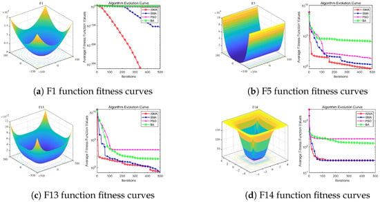
Furthermore, to provide a clearer comparison of performance across different methods, we plot their convergence trajectories based on the experimental data. This allows for a precise assessment of their convergence behavior on the test suite. Figure 6 illustrates the optimization progress of ISMA, SMA, PSO, and BA on selected benchmarks. It is visually evident from the plots that ISMA surpasses the competing algorithms regarding both convergence speed and solution precision.

Figure 6. Fitness curves of ISMA, SMA, PSO, and BA methods for test function optimization process.

4.3. Performance of ISMA-HKELM on Datasets

NASA datasets and CALCE datasets are selected for the experiments. The predicted results are compared with those of Long Short-Term Memory (LSTM) [52], Support Vector Machine (SVM) [53], and SMA-HKELM. The key parameters of the prediction model in the experiment are presented in Table 3.

Table 3. Parameterization of the prediction method.

Prediction Method	Parameter Setting
ISMA-HKELM	$\mathrm{pop}=50$; $\text{Max\_iter}=1000$, $g(·)=\mathrm{Sigmoidal}$
SMA-HKELM	$\mathrm{pop}=10$; $\text{Max\_iter}=1000$, $g(·)=\mathrm{Sigmoidal}$
LSTM	$\mathrm{Epochs}=1000$ $\mathrm{Ir}=0.005$
SVM	epsilon−SVM, polynomial

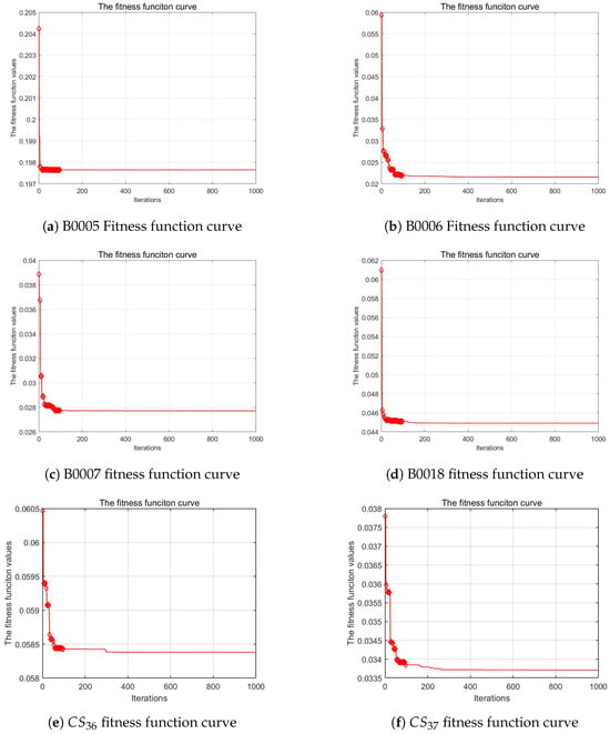
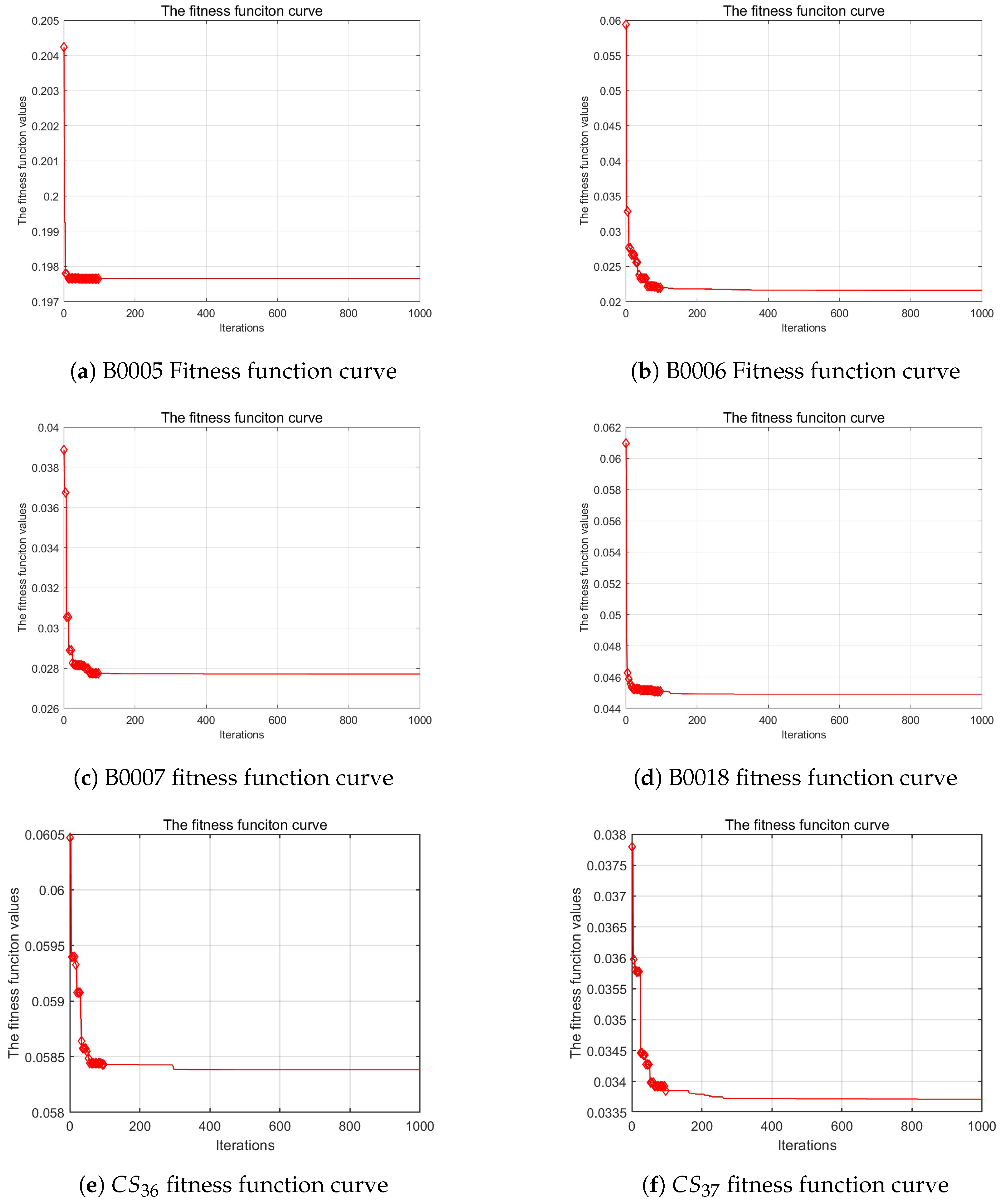
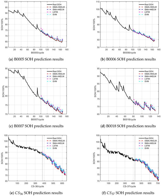
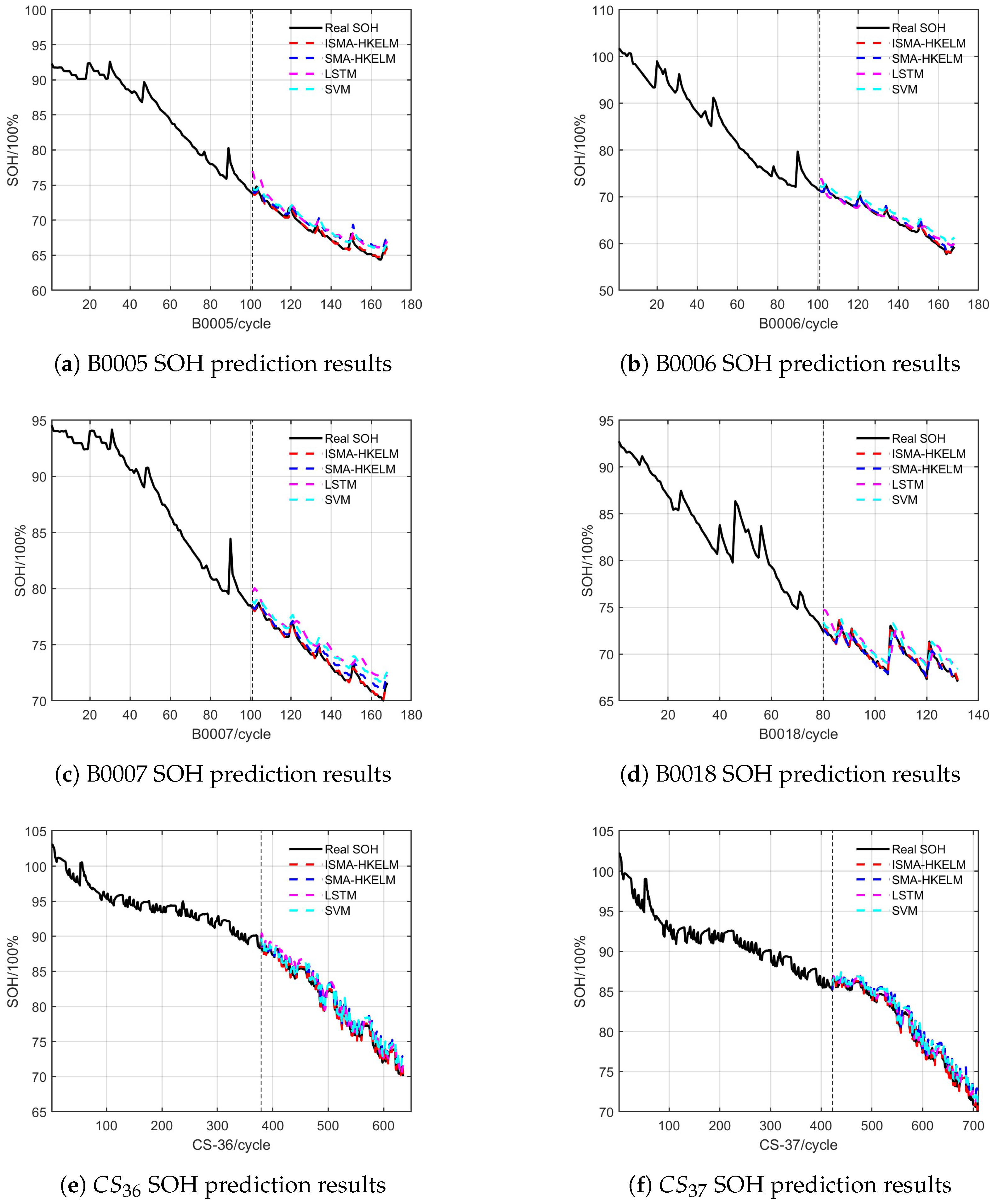
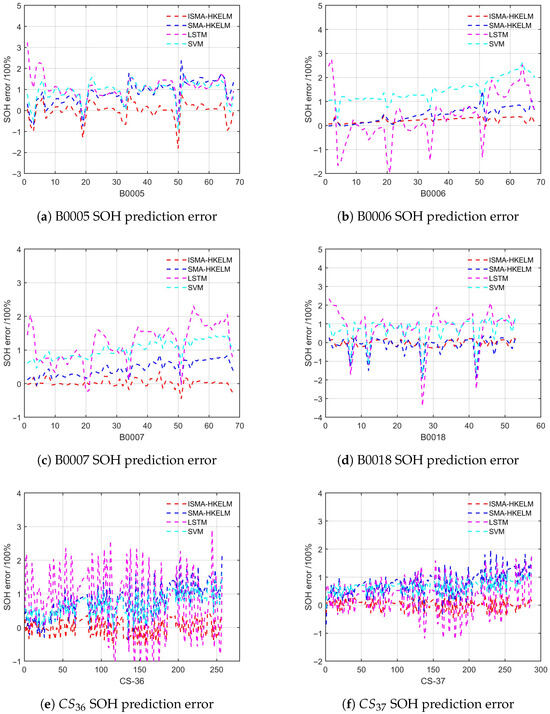
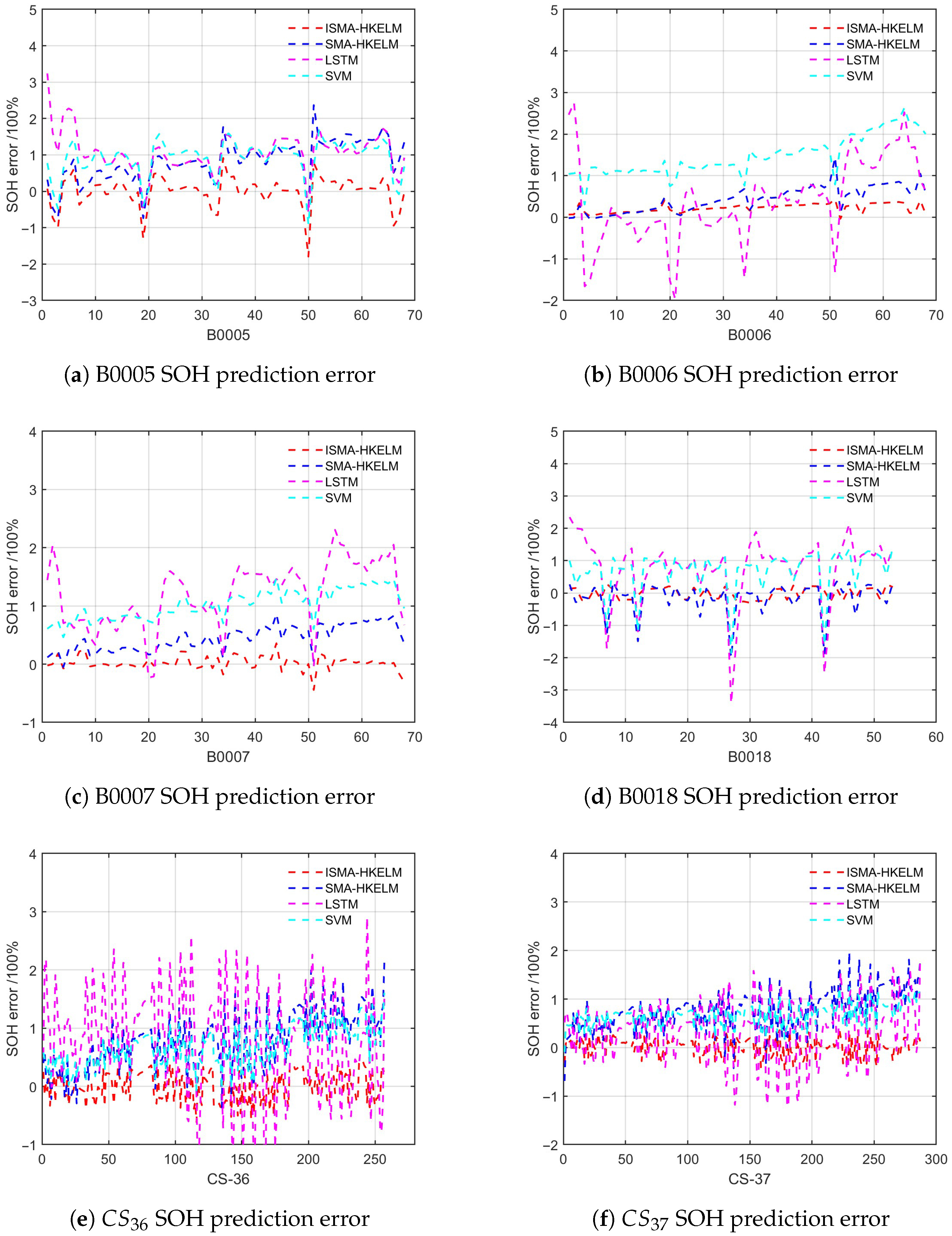
The training phase utilized 60% of the total cycle dataset. Figure 7 displays the progression of fitness values for every battery instance. Figure 8 provides a visual comparison of the prediction results generated by ISMA-HKELM against LSTM, SVM, and SMA-HKELM, whereas Figure 9 highlights the absolute error margins between the estimated outputs and the actual data. A detailed summary of the evaluation metrics for all four algorithms is provided in Table 4. As observed in Figure 7, the ISMA-HKELM fitness curve stabilizes rapidly as iterations progress, demonstrating the algorithm’s swift convergence capability. A comprehensive analysis of SOH prediction performance across all LIB models reveals that ISMA-HKELM consistently secures the best results in terms of MAE, MBE, RMSE, and $R^2$.

Figure 7. Fitness function of battery data for each model.

Figure 8. SOH prediction results for each type of LIB.

Figure 9. SOH prediction error for each type of LIB.

Table 4. Data on evaluation indicators of the results of the forecasting methodology.

No.	Model	MAE	MBE	RMSE	${\mathit{R}}^2$
B0005	ISMA-HKELM	0.3012	0.0056	0.4481	0.9742
	SMA-HKLEM	0.9241	0.8445	1.0265	0.8644
	LSTM	1.276	0.6682	1.4648	0.5914
	SVM	0.9787	0.9116	1.1413	0.9614
B0006	ISMA-HKELM	0.2309	0.2276	0.2535	0.9959
	SMA-HKLEM	1.9649	1.1094	2.2315	0.3222
	LSTM	1.2713	0.9553	1.5479	0.8292
	SVM	1.2612	1.2634	1.6003	0.9114
B0007	ISMA-HKELM	0.1013	−0.0092	0.1222	0.9974
	SMA-HKLEM	0.7247	0.1965	0.9347	0.6440
	LSTM	0.9109	0.8442	1.0304	0.8072
	SVM	1.1231	1.2014	1.1002	0.9018
B0018	ISMA-HKELM	0.1820	−0.0156	0.1877	0.9874
	SMA-HKLEM	0.5985	−0.1792	0.8238	0.6778
	LSTM	1.1265	0.5859	1.346	0.3473
	SVM	0.9884	0.8124	0.9813	0.7466
CS2_36	ISMA-HKELM	0.2085	0.0067	0.2425	0.9979
	SMA-HKLEM	0.7796	0.7635	0.8954	0.9719
	LSTM	1.8937	0.6001	2.3118	0.7724
	SVM	0.7819	0.7724	0.8610	0.9812
CS2_37	ISMA-HKELM	0.1544	0.0304	0.1841	0.9986
	SMA-HKLEM	0.7949	0.78651	0.87636	0.9674
	LSTM	1.3633	1.2768	1.6502	0.8662
	SVM	0.8095	0.7705	0.8124	0.9882

Using the B0005 battery model as a case study, the enhanced ISMA-HKELM framework exhibits substantial gains over the standard SMA-HKELM approach across all key indicators. Specifically, MAE decreased by 66.34%, MBE by 99.02%, and RMSE by 55.49%, while the $R^2$ score increased by 11.31%. These statistics clearly underscore the efficacy of ISMA in hyperparameter optimization and verify the superior prediction accuracy achieved by the ISMA-HKELM model.

Predictive analysis on LIB B0005 demonstrates that the improved ISMA-HKELM model significantly outperforms the SMA-HKELM model across all performance metrics. Specifically, the model achieved reductions of $66.34\%$ in MAE, $99.02\%$ in MBE, and $55.49\%$ in RMSE, along with an $11.31\%$ improvement in $R^2$. These results compellingly evidence the superior capability of ISMA in parameter optimization and fully validate the substantial enhancement in prediction accuracy offered by the proposed model.

The average values of MAE, MBE, RMSE, and $R^2$ predicted by six LIB models using the four models were calculated. It was found that the average MAE of ISMA-HKELM decreased by 68.45% compared to that of SMA-HKELM; the average MAE of ISMA-HKELM decreased by 76.07% compared to LSTM; the average MAE of ISMA-HKELM decreased by 80% compared to the average MAE of SVM.

In terms of average MBE comparison, the average MBE of ISMA-HKELM is 91.39% lower than the average MBE of SMA-HKELM, 91.2% lower than the average MBE of LSTM, and 94.73% lower than the average MBE of SVM.

In terms of average RMSE, the average RMSE of ISMA-HKELM decreased by 66.87% compared to the average RMSE of SMA-HKELM, the average RMSE of ISMA-HKELM decreased by 75.43% compared to the average RMSE of LSTM, and the average RMSE of ISMA-HKELM decreased by 76.56% compared to the average RMSE of SVM.

In terms of average $R^2$, the average $R^2$ of ISMA-HKELM is improved by 5.19% over the average $R^2$ of SMA-HKELM, 13.47% over the average $R^2$ of LSTM, and 16% over the average $R^2$ of SVM. This result fully demonstrates the excellent performance of ISMA-HKELM on a variety of datasets and further confirms the algorithm’s generalization ability and robustness.

4.4. Discussion

Computational Complexity and Real-time Feasibility: The proposed ISMA-HKELM model, once trained, exhibits extremely low computational complexity during the inference phase. Unlike deep learning models (e.g., LSTM) that require recursive matrix operations, HKELM is a feedforward network where prediction involves only simple matrix multiplications. The average inference time per sample is less than 1ms on a standard CPU, making it highly suitable for real-time deployment in Battery Management Systems (BMSs) with limited computational resources. Although the offline training process involves ISMA optimization, this is a one-time cost that does not affect online performance.

Robustness Analysis: The robustness of the model is validated through its consistent performance across two distinct datasets (NASA and CALCE) with different battery chemistries and operating conditions. The use of the Hybrid Kernel (RBF + Poly) allows the model to capture both local variations and global trends, effectively mitigating the impact of measurement noise and partial data. The low standard deviations observed in the repeated validation experiments (Table 4) further confirm that the model is insensitive to initial conditions and stochastic fluctuations, ensuring reliable operation in practical scenarios.

Future Work: While this study focuses on two key health indicators (HF1, HF2), future research could explore the integration of additional features (e.g., temperature, incremental capacity analysis peaks) to further enhance prediction accuracy under extreme conditions. However, a trade-off between feature complexity and computational cost must be carefully maintained for BMS applications.

5. Conclusions

This study presents the ISMA-HKELM framework, designed to provide precise SOH estimation for LIBs across their full operational lifespan.

The process starts by confirming the relationship between indirect health indicators and SOH via a comprehensive correlation analysis using NASA and CALCE datasets. Following this, ISMA is utilized to conduct a fine-grained optimization of the Hybrid Kernel Extreme Learning Machine (HKELM). Key hyperparameters targeted for tuning include the regularization term, kernel weights, and the variance of the RBF kernel, as well as the polynomial kernel’s bias and degree. By leveraging the optimal parameter set derived from this extensive search, the ISMA-HKELM predictor is established to guarantee high-accuracy SOH forecasting.

To fully assess the ISMA-HKELM model’s capabilities, we gathered data from six distinct LIB types. The forecasting performance of ISMA-HKELM was then benchmarked against LSTM, SVM, and the standard SMA-HKELM. The evaluation, relying on MAE, MBE, RMSE, and the coefficient of determination (${\mathit{R}}^{\mathbf{2}}$), clearly shows that ISMA-HKELM surpasses the other three methods across all metrics, thereby validating its superior accuracy and generalization potential.

References

- Scrosati, B.; Hassoun, J.; Sun, Y.K. Lithium-ion batteries. A look into the future. Energy Environ. Sci. 2011, 4, 3287–3295. [Google Scholar] [CrossRef] [Scilit]
- Zubi, G.; Dufo-López, R.; Carvalho, M.; Pasaoglu, G. The lithium-ion battery: State of the art and future perspectives. Renew. Sustain. Energy Rev. 2018, 89, 292–308. [Google Scholar] [CrossRef] [Scilit]
- Hosen, M.S.; Jaguemont, J.; Van Mierlo, J.; Berecibar, M. Battery lifetime prediction and performance assessment of different modeling approaches. iScience 2021, 24, 102060. [Google Scholar] [CrossRef] [Scilit]
- Zhang, F.; Hu, X.; Langari, R.; Cao, D. Energy management strategies of connected HEVs and PHEVs: Recent progress and outlook. Prog. Energy Combust. Sci. 2019, 73, 235–256. [Google Scholar] [CrossRef] [Scilit]
- Chen, Y.; Kang, Y.; Zhao, Y.; Wang, L.; Liu, J.; Li, Y.; Liang, Z.; He, X.; Li, X.; Tavajohi, N.; et al. A review of lithium-ion battery safety concerns: The issues, strategies, and testing standards. J. Energy Chem. 2021, 59, 83–99. [Google Scholar] [CrossRef] [Scilit]
- Chen, M.; Ma, G.; Liu, W.; Zeng, N.; Luo, X. An overview of data-driven battery health estimation technology for battery management system. Neurocomputing 2023, 532, 152–169. [Google Scholar] [CrossRef] [Scilit]
- Mingant, R.; Bernard, J.; Moynot, V.S.; Delaille, A.; Mailley, S.; Hognon, J.L.; Huet, F. EIS measurements for determining the SOC and SOH of Li-ion batteries. Electrochem. Soc. Trans. 2011, 33, 41–53. [Google Scholar] [CrossRef] [Scilit]
- Lee, J.; Won, J. Enhanced coulomb counting method for SoC and SoH estimation based on coulombic efficiency. IEEE Access 2023, 11, 15449–15459. [Google Scholar] [CrossRef] [Scilit]
- Bian, X.; Wei, Z.; Li, W.; Pou, J.; Sauer, D.U.; Liu, L. State-of-health estimation of lithium-ion batteries by fusing an open circuit voltage model and incremental capacity analysis. IEEE Trans. Power Electron. 2021, 37, 2226–2236. [Google Scholar] [CrossRef] [Scilit]
- Wang, R.; Li, J.; Wang, X.; Wang, S.; Pecht, M. Deep learning model for state of health estimation of lithium batteries based on relaxation voltage. J. Energy Storage 2024, 79, 110189. [Google Scholar] [CrossRef] [Scilit]
- Wei, Z.; Hu, J.; He, H.; Yu, Y.; Marco, J. Embedded Distributed Temperature Sensing Enabled Multistate Joint Observation of Smart Lithium-Ion Battery. IEEE Trans. Ind. Electron. 2023, 70, 555–565. [Google Scholar] [CrossRef] [Scilit]
- Obeid, H.; Petrone, R.; Chaoui, H.; Gualous, H. Higher order sliding-mode observers for state-of-charge and state-of-health estimation of lithium-ion batteries. IEEE Trans. Veh. Technol. 2022, 72, 4482–4492. [Google Scholar] [CrossRef] [Scilit]
- Huang, Z.; Best, M.; Knowles, J.; Fly, A. Adaptive piecewise equivalent circuit model with SOC/SOH estimation based on extended Kalman filter. IEEE Trans. Energy Convers. 2022, 38, 959–970. [Google Scholar] [CrossRef] [Scilit]
- Guo, W.; Wang, Q.; Li, G.; Xie, S. Dual-time scale collaborative estimation of SOC and SOH for lithium-ion batteries based on FOMIRUKF-EKF. Comput. Electr. Eng. 2025, 123, 110048. [Google Scholar] [CrossRef] [Scilit]
- Liu, W.; Xu, Y. Data-driven online health estimation of Li-ion batteries using a novel energy-based health indicator. IEEE Trans. Energy Convers. 2020, 35, 1715–1718. [Google Scholar] [CrossRef] [Scilit]
- Chaoui, H.; Ibe-Ekeocha, C.C. State of charge and state of health estimation for lithium batteries using recurrent neural networks. IEEE Trans. Veh. Technol. 2017, 66, 8773–8783. [Google Scholar] [CrossRef] [Scilit]
- Pan, H.; Lü, Z.; Wang, H.; Wei, H.; Chen, L. Novel battery state-of-health online estimation method using multiple health indicators and an extreme learning machine. Energy 2018, 160, 466–477. [Google Scholar] [CrossRef] [Scilit]
- Ge, D.; Jin, G.; Wang, J.; Zhang, Z. A novel data-driven IBA-ELM model for SOH/SOC estimation of lithium-ion batteries. Energy 2024, 305, 132395. [Google Scholar] [CrossRef] [Scilit]
- Zhang, C.y.; Wang, S.l.; Yu, C.m.; Xie, Y.x.; Fernandez, C. Improved particle swarm optimization-extreme learning machine modeling strategies for the accurate lithium-ion battery state of health estimation and high-adaptability remaining useful life prediction. J. Electrochem. Soc. 2022, 169, 080520. [Google Scholar] [CrossRef] [Scilit]
- Cai, L.; Meng, J.; Stroe, D.I.; Peng, J.; Luo, G.; Teodorescu, R. Multiobjective optimization of data-driven model for lithium-ion battery SOH estimation with short-term feature. IEEE Trans. Power Electron. 2020, 35, 11855–11864. [Google Scholar] [CrossRef] [Scilit]
- Guo, Y.; Yang, D.; Zhang, Y.; Wang, L.; Wang, K. Online estimation of SOH for lithium-ion battery based on SSA-Elman neural network. Prot. Control Mod. Power Syst. 2022, 7, 1–17. [Google Scholar] [CrossRef] [Scilit]
- Wen, J.; Chen, X.; Li, X.; Li, Y. SOH prediction of lithium battery based on IC curve feature and BP neural network. Energy 2022, 261, 125234. [Google Scholar] [CrossRef] [Scilit]
- Islam, S.; Namkoong, G. High-Fidelity SOH Prediction in Lithium-Ion Batteries Using Hybrid ML Networks. J. Electrochem. Soc. 2025, 172, 080506. [Google Scholar] [CrossRef] [Scilit]
- Liu, S.; Chen, Z.; Yuan, L.; Xu, Z.; Jin, L.; Zhang, C. State of health estimation of lithium-ion batteries based on multi-feature extraction and temporal convolutional network. J. Energy Storage 2024, 75, 109658. [Google Scholar] [CrossRef] [Scilit]
- Xu, P.; Li, H.; Cao, F.; Peng, X.; Wang, X.; Ran, W.; Wan, S. State of Health Estimation Method for Lithium-Ion Batteries Based on BiLSTM-Transformer and Fusion Features. J. Electrochem. Soc. 2025, 172, 100501. [Google Scholar] [CrossRef] [Scilit]
- Yin, Y.; Gao, Z.; Huang, Y.; Liu, Q. PLT-GRU: Physics-informed lightweight Transformer-GRU algorithm for few-shot battery state-of-health estimation. Meas. Sci. Technol. 2025, 36, 096216. [Google Scholar] [CrossRef] [Scilit]
- Zhang, Y.; Ge, X.; Li, X.; Zhao, F.; Zhang, K.; Zhong, W. SOH Prediction of High-Capacity Lithium-Ion Batteries under High-Rate Charging via a TCN-BiGRU Model with Multi-Head Attention. J. Electrochem. Soc. 2025, 172, 100516. [Google Scholar] [CrossRef] [Scilit]
- Xue, T.; Li, X.; Xi, L.; Zhang, J. Lithium battery SOH prediction based on frequency-enhanced cross variable for short-term dependency recognition framework. Meas. Sci. Technol. 2025, 36, 066001. [Google Scholar] [CrossRef] [Scilit]
- Dang, S.; Sun, B.; Zhang, W.; Tao, Y.; Li, J. A transfer learning and graph neural network-based method for SOH prediction of lithium-ion batteries in energy storage systems. Meas. Sci. Technol. 2025, 36, 106128. [Google Scholar] [CrossRef] [Scilit]
- Hoarfrost, A.; Aptekmann, A.; Farfañuk, G.; Bromberg, Y. Deep learning of a bacterial and archaeal universal language of life enables transfer learning and illuminates microbial dark matter. Nat. Commun. 2022, 13, 2606. [Google Scholar] [CrossRef] [Scilit] [PubMed]
- Huang, H.; Bian, C.; Wu, M.; An, D.; Yang, S. A novel integrated SOC–SoH estimation framework for whole-life-cycle lithium-ion batteries. Energy 2024, 288, 129801. [Google Scholar] [CrossRef] [Scilit]
- Zhao, J.; Liu, M.; Zhang, B.; Wang, X.; Liu, D.; Wang, J.; Bai, P.; Liu, C.; Sun, Y.; Zhu, Y. Review of Lithium-Ion Battery Fault Features, Diagnosis Methods, and Diagnosis Procedures. IEEE Internet Things J. 2024, 11, 18936–18950. [Google Scholar] [CrossRef] [Scilit]
- Fei, Z.; Zhang, Z.; Tsui, K.L. Deep learning powered online battery health estimation considering multitimescale aging dynamics and partial charging information. IEEE Trans. Transp. Electrif. 2024, 10, 1256–1268. [Google Scholar] [CrossRef] [Scilit]
- Zou, B.; Xiong, M.; Wang, H.; Ding, W.; Jiang, P.; Hua, W.; Zhang, Y.; Zhang, L.; Wang, W.; Tan, R. A deep learning approach for state-of-health estimation of lithium-ion batteries based on a multi-feature and attention mechanism collaboration. Batteries 2023, 9, 329. [Google Scholar] [CrossRef] [Scilit]
- Wang, W.; Yang, K.; Zhang, L.; Zhou, S.; Ren, B.; Lu, Y.; Tan, R.; Zhu, T.; Ma, B.; Yang, S.; et al. An end-cloud collaboration approach for online state-of-health estimation of lithium-ion batteries based on multi-feature and transformer. J. Power Sources 2024, 608, 234669. [Google Scholar] [CrossRef] [Scilit]
- Liu, X.; Yang, K.; Zou, B.; Zhang, X.; Bao, G.; Ma, B.; Zhang, L.; Tan, R. Accurate estimation of state of health for lithium-ion batteries based on Pyraformer and TimeGAN data augmentation. J. Power Sources 2025, 640, 236722. [Google Scholar] [CrossRef] [Scilit]
- Ma, G.; Xu, S.; Yang, T.; Du, Z.; Zhu, L.; Ding, H.; Yuan, Y. A transfer learning-based method for personalized state of health estimation of lithium-ion batteries. IEEE Trans. Neural Netw. Learn. Syst. 2024, 35, 1890–1902. [Google Scholar] [CrossRef] [Scilit]
- Lu, J.; Xiong, R.; Tian, J.; Wang, C.; Sun, F. Deep learning to estimate lithium-ion battery state of health without additional degradation experiments. Nat. Commun. 2023, 14, 2760. [Google Scholar] [CrossRef] [Scilit]
- Hu, J.; Fu, P.; Wei, Z.; Huang, Y.; Early, J.; Fly, A.; Zhang, Y. Early prediction of lithium-ion battery degradation with a generative pre-trained transformer. Nat. Commun. 2025, 17, 126. [Google Scholar] [CrossRef] [Scilit]
- Huang, G.B.; Zhu, Q.Y.; Siew, C.K. Extreme learning machine: A new learning scheme of feedforward neural networks. In Proceedings of the 2004 IEEE International Joint Conference on Neural Networks (IEEE Cat. No. 04CH37541); IEEE: Piscataway, NJ, USA, 2004; Volume 2, pp. 985–990. [Google Scholar]
- Alsuwian, T.; Ansari, S.; Zainuri, M.A.A.M.; Ayob, A.; Hussain, A.; Lipu, M.H.; Alhawari, A.R.; Almawgani, A.; Almasabi, S.; Hindi, A.T. A review of expert hybrid and co-estimation techniques for SOH and RUL estimation in battery management system with electric vehicle application. Expert Syst. Appl. 2024, 246, 123123. [Google Scholar] [CrossRef] [Scilit]
- Yang, S.; Qin, H.; Liu, Z.; He, B.; Li, G. An efficient state-of-health estimation method for lithium-ion batteries based on feature-importance ranking strategy and hybrid kernel extreme learning machine algorithm. J. Energy Storage 2024, 103, 114260. [Google Scholar] [CrossRef] [Scilit]
- Saha, B.; Goebel, K. Battery Data Set, NASA Ames Prognostics Data Repository; NASA Ames Research Center: Moffett Field, CA, USA, 2007.
- He, W.; Williard, N.; Osterman, M.; Pecht, M. Prognostics of lithium-ion batteries based on Dempster–Shafer theory and the Bayesian Monte Carlo method. J. Power Sources 2011, 196, 10314–10321. [Google Scholar] [CrossRef] [Scilit]
- Li, S.; Chen, H.; Wang, M.; Heidari, A.A.; Mirjalili, S. Slime mould algorithm: A new method for stochastic optimization. Future Gener. Comput. Syst. 2020, 111, 300–323. [Google Scholar] [CrossRef] [Scilit]
- Naik, M.K.; Panda, R.; Abraham, A. Adaptive opposition slime mould algorithm. Soft Comput. 2021, 25, 14297–14313. [Google Scholar] [CrossRef] [Scilit]
- Gao, S.; Li, Z.; Zhang, Y.; Zhang, S.; Zhou, J. Remaining useful life prediction method of rolling bearings based on improved 3σ and DBO-HKELM. Meas. Sci. Technol. 2024, 35, 106101. [Google Scholar] [CrossRef] [Scilit]
- Müller, K.R.; Mika, S.; Tsuda, K.; Schölkopf, K. An introduction to kernel-based learning algorithms. In Handbook of Neural Network Signal Processing; CRC Press: Boca Raton, FL, USA, 2018; pp. 1–4. [Google Scholar]
- Huang, G.B.; Zhu, Q.Y.; Siew, C.K. Extreme learning machine: Theory and applications. Neurocomputing 2006, 70, 489–501. [Google Scholar] [CrossRef] [Scilit]
- Kennedy, J.; Eberhart, R. Particle swarm optimization. In Proceedings of the ICNN’95-International Conference on Neural Networks; IEEE: Piscataway, NJ, USA, 1995; Volume 4, pp. 1942–1948. [Google Scholar]
- Cruz, C.; González, J.R.; Pelta, D.A.; Krasnogor, N.; Terrazas, G. Nature Inspired Cooperative Strategies for Optimization (NICSO 2010); Springer: Berlin/Heidelberg, Germany, 2010; Volume 284. [Google Scholar]
- Hochreiter, S.; Schmidhuber, J. Long short-term memory. Neural Comput. 1997, 9, 1735–1780. [Google Scholar] [CrossRef] [Scilit]
- Hearst, M.A.; Dumais, S.T.; Osuna, E.; Platt, J.; Scholkopf, B. Support vector machines. IEEE Intell. Syst. Their Appl. 1998, 13, 18–28. [Google Scholar] [CrossRef] [Scilit]
Disclaimer/Publisher’s Note: The statements, opinions and data contained in all publications are solely those of the individual author(s) and contributor(s) and not of MDPI and/or the editor(s). MDPI and/or the editor(s) disclaim responsibility for any injury to people or property resulting from any ideas, methods, instructions or products referred to in the content. |
© 2026 by the authors. Licensee MDPI, Basel, Switzerland. This article is an open access article distributed under the terms and conditions of the Creative Commons Attribution (CC BY) license.