A Method for Identifying Power Quality Disturbances Based on Adaptive KS Transform and Multimodal Feature Fusion

Abstract

With the scale of new energy access expanding, the proportion of nonlinear loads in the power grid has increased, leading to frequent impact disturbance events. The types of power quality disturbances (PQDs) are becoming increasingly complex, placing greater demands on the accurate identification of disturbance signals. Therefore, this paper proposes a PQD recognition method based on adaptive KS transform and a Multimodal Feature Fusion Network (MFNet). Firstly, using an improved red-billed blue magpie optimization algorithm, the traditional KS transform window function parameters are adaptively optimized to achieve accurate time–frequency localization of PQD. Secondly, considering the differential characteristics of PQDs in different modes, combined with the proposed adaptive KS transform, a parallel MFNet with three branches in the time domain, frequency domain, and time–frequency domain is constructed; to further enhance feature extraction capability and reduce information loss, residual structures are introduced in the network. Multiple comparative experimental results show that the proposed method achieves an average classification accuracy of 99.52% at 20 dB of noise and demonstrates good noise resistance.

1. Introduction

The safe and stable operation of a power system is an important indicator for measuring the level of power grid operation and power supply quality [1]. With widespread access to renewable energy and the rapid development of power electronic devices, nonlinear and impulsive loads in the power grid have increased significantly, leading to a range of power quality problems [2]. Moreover, the accurate detection of PQDs is essential for maintaining the operational stability and resilience of modern energy systems, such as multi-microgrids integrated with electric vehicles, especially when facing extreme weather conditions [3]. These complex problems mainly manifest as a composite of various disturbances, which significantly increase the difficulty of identification under multi-scale feature variations [4]. The existence of PQDs not only seriously affects end-user experience but also endangers the safe and economic operation of the power grid [5]. Therefore, in order to improve power quality and promote the development of smart grids, there is an urgent need for an effective PQD identification method.

PQD recognition can usually be divided into two steps, namely feature extraction and classification [6]. In the process of feature extraction, signal transformation-based feature extraction methods are often used to characterize PQD characteristics from different modal perspectives [7], and recognition performance is improved by optimizing feature representation and key parameter settings [8]. In terms of time-domain (TD) modes, methods such as wavelet packet decomposition, Hilbert–Huang Transform (HHT) [9], and Empirical Mode Decomposition (EMD) [10] can reflect the instantaneous variation characteristics of disturbances and capture information such as waveform mutations and amplitude changes [11]. Among them, EMD has a good local time-domain analytical ability by adaptively decomposing the signal into several intrinsic mode functions [12]. In terms of frequency-domain (FD) modes, Fourier transform and its improved methods have long been used for frequency component analysis of steady-state signals, but their ability to express non-stationary disturbances is limited [13]. Short-Time Fourier Transform (STFT) introduces a window function on this basis to extract local spectra and has been widely used in the identification of periodic disturbances and harmonic waves [14]. In terms of time–frequency (TF) modes, Discrete Wavelet Transform (DWT) [15], Stockwell Transform (ST) and its improved methods (Modified ST, MST) [16] can characterize the distribution of signal energy in time and frequency and are used to describe the evolution process of non-stationary disturbances [17]. Among them, ST and its improved algorithms are widely used due to their good flexibility and time–frequency positioning ability. However, when ST uses Gaussian windows to extract PQD time–frequency information, it is difficult to balance time–frequency resolution, and energy concentration is limited [18]. To address the above shortcomings, ref. [19] proposes a Kaiser window-based ST (KS Transform, KST) to replace Gaussian windows. Despite its superior energy concentration, the performance of KST is heavily dependent on the empirical setting of window parameters. This lack of adaptivity often results in information loss or “blurred” features when dealing with non-stationary composite disturbances, creating a research gap in high-precision feature characterization for volatile grid environments.

In the classification process, existing methods can be mainly divided into two categories [20]: one is traditional machine learning methods, which are usually based on manually constructed features and input into classifiers to complete discrimination [21,22]. This method is relatively simple to implement, but it relies heavily on feature design and parameter selection, and its performance is easily affected by changes in operating conditions or increased noise [23]. Another type is deep learning methods, especially Convolutional Neural Networks (CNNs), which can achieve end-to-end feature learning and have received widespread attention in PQD recognition [24]. Ref. [25] designed a one-dimensional CNN combined with the EMD time-domain modal features of disturbance signals for PQD classification, achieving good classification results. Reference [26] proposed a dual-branch network combining one-dimensional and two-dimensional CNNs for joint modeling of two modal features of PQDs, which showed excellent performance in PQD detection. However, a critical limitation of existing methods is their inability to fully capture the complex process information of non-stationary signals. Inspired by recent advancements in deep fractional multidimensional spectrum fusion [27] and multi-domain feature collaborative representation [28], constructing a framework that integrates differentiated information across multiple modalities has become a pivotal direction for overcoming the “feature sparsity” problem in complex PQD recognition.

To address the aforementioned issues, this paper proposes a power quality disturbance identification method based on adaptive KS transform (AKST) and a Multimodal Feature Fusion Network (MFNet). The logical connection of our work is built upon solving the rigidity of fixed-parameter transforms and the information deficiency of low-dimensional features. The main contributions of this article are as follows:

To solve the problem of poor adaptability in traditional time–frequency analysis, an ARBMO-based parameter-adaptive strategy is introduced to optimize the KS transform window. This improves energy focusing and localization accuracy, ensuring stable feature extraction even under complex and noisy working conditions.

To overcome the information loss inherent in single-modal recognition, a multimodal feature fusion framework (MFNet) is constructed. By aligning and fusing three-branch features (EMD, STFT, and AKST) in a parallel architecture, the network achieves a unified, comprehensive representation of PQD signals.

The proposed method is tested against 30 types of disturbances to check its engineering practicality and robustness. Results show strong performance even under extreme noise and hardware-in-the-loop testing. The method outperforms existing benchmarks in accuracy and reliability.

2. Time–Frequency Analysis Based on Adaptive KS Transform

2.1. KS Transformation Principle

The time–frequency characteristic information of PQDs is crucial for accurate identification of PQDs. Therefore, high-frequency resolution and energy concentration are needed to reduce information loss. In reference [19], KST for time–frequency analysis is proposed, which is defined as

$$KS(\tau ,f)={{\displaystyle \int }}_{-\infty }^{+\infty }x(t)w_k(\tau -t,f)e^{-j2\pi ft}dt$$

(1)

where $x(t)$ represents the PQD signal, $t$ represents time, $\tau$ represents the time shift factor, $f$ represents signal frequency, $j$ represents the imaginary unit, and $w_k(t,f)$ represents the Kaiser window function, i.e.,

$$w_k(t,f)={\displaystyle \frac{I_0\left[\alpha (\sqrt{1-{(t/T)}^2}\right]}{I_0[\alpha ]}},|t|\le T$$

(2)

where $I_0(·)$ is the first type of zero-order Bessel function, and its power series expansion is defined as

$$I_0(·)=1+{\displaystyle \sum }_{m=1}^{\infty }\left[{\displaystyle \frac{{(·/2)}^m}{m!}}\right]$$

(3)

In Equation (2), $\alpha$ is a frequency-dependent control function used to adjust the shape of the Kaiser window and $T$ is the time-scale parameter. The control function $\alpha$ is the most critical parameter of the Kaiser window, as it determines the trade-off between the main-lobe width and the side-lobe level. According to the Kaiser window theory, the relationship between $\alpha$ and the side-lobe attenuation $\gamma$ (in dB) is governed by the following piecewise logic:

$$\alpha =\left\{\begin{array}{c}0.1102(\gamma -8.7),\gamma \ge 50\\ 0.5482{(\gamma -21)}^{0.4}+0.07886(\beta -21),21<\gamma <50\\ \begin{array}{l}0,\gamma \le 21\hfill \end{array}\end{array}\right.$$

(4)

By adjusting $\alpha$, the window can adaptively transition between different characteristics. For instance, when $\alpha =0$, the Kaiser window degrades into a rectangular window; when $\alpha =4.86$, it approximates a Hamming window; and when $\alpha =7.04$, it approximates a Blackman window. To provide good time–frequency resolution, the design in reference [19] is as follows:

$$\alpha (f)=\lambda f$$

(5)

where $\lambda$ is used to control the change in window shape.

2.2. AKST Method Based on Dynamic Parameter Optimization

KST has better a time–frequency performance than ST based on Gaussian windows [5]. However, the fixed $\lambda$ limits its adaptation to PQDs, thereby reducing resolution. To this end, this article further proposes AKST, which optimizes the control function $\alpha (f)$ by introducing an adjustment factor $a,p,b$, thereby adjusting the rate of change in window shape and improving its adaptability to PQDs. The new control function is defined as

$$\beta (f)=a{f}^p+b$$

(6)

where $p\in (0,1)$; specifically, when $p=1$ and $b=0$, $\beta (f)$ is equal to the original control function $\alpha (f)$.

According to the control function $\beta (f)$, the adaptive KS transformation can be defined as

$$\begin{array}{l}AKS(\tau ,f)=\hfill \\ {{\displaystyle \int }}_{-\infty }^{\infty }x(t){\displaystyle \frac{I_0\left[\beta (f)\sqrt{1-{((t-\tau )/T)}^2}\right]}{I_0[\beta (f)]}}{e}^{-j2\pi ft}dt\hfill \end{array}$$

(7)

In the experiment, the sampling frequency and sampling points are set to $f_s$ and $N$, respectively, and the sampling time interval can be calculated as $T_s=1/f_s$. The PQD signal $x(t)$ is converted into a discrete signal $X(n)$ after sampling and processing. In this paper, the range of $m$ values is set from 0 to $N-1$ to adjust the time shift. Among them, $\tau =m{T}_s$ and $f=n/N{T}_s$. When $n>0$$(n=0,\dots ,N-1)$, the discrete AKST of $X(n)$ can be described as

$$AKS(m,n)={\displaystyle \sum }_{r=0}^{N-1}X(n+r)W_K(n)e^{j{\displaystyle \frac{2\pi mr}{N}}}$$

(8)

where $X(n+r)$ and $W_K(n)$ are the discrete Fourier transform results of $X(n)$ and Kaiser window $w^{\prime }(f)$, respectively. The value of r ranges from 0 to $n-1$ and is used to control the translation length of $X(n)$.

Among them, $AKS(m,n)$ is a two-dimensional complex matrix. Therefore, Equation (6) can be further expressed as

$$AKS(m,n)=|AKS(m,n)|e^{j\varphi (m,n)}$$

(9)

where $|AKS(m,n)|$ and $\varphi (m,n)$ respectively represent the amplitude and phase angle of $AKS(m,n)$.

In order to dynamically adjust the parameters of the control function driven by (6), this paper adopts the discrete AKST energy concentration measurement as the optimization index, and its expression is

$$E_{AKS}\left(a,p,b\right)={\displaystyle \frac{1}{{{\displaystyle \sum }}_{m=1}^M{{\displaystyle \sum }}_{n=1}^N\left|\frac{AKS(m,n)}{\sqrt{\sum \sum |AKS(m,n){|}^2}}\right|}}$$

(10)

where the size of matrix $AKS(m,n)$ is $M\times N$.

Energy concentration quantifies the time–frequency aggregation of energy. To reduce energy leakage and enhance feature saliency, we maximize energy concentration and adaptively optimize the $a,p,b$ parameter as follows:

$$\underset{a,p,b}{\arg \max =}\left\{E_{AKS}\left(a,p,b\right)\right\}$$

(11)

To solve the above optimization problem, this paper introduces the Red-billed Blue Magpie Optimizer (RBMO) algorithm [29]. This algorithm simulates the collaborative predation behavior of red-billed blue magpies in natural environments, utilizing information sharing and collaboration among individuals to achieve a balance between global and local search. It has advantages such as fast convergence speed and strong robustness.

However, the standard RBMO has a fixed Concentration Factor (CF) and balance factor $\epsilon$, which tend to converge to local optima earlier in multi-parameter optimization, making it difficult to achieve optimal results. In response to the above shortcomings, this paper proposes the Adaptive Red-billed Blue Magpie Optimizer (ARBMO) algorithm, which is based on the RBMO and uses the energy-aggregation function of discrete AKST as the fitness function. By introducing adaptive adjustment coefficients, the efficiency of parameter optimization is improved. Referring to the optimization function in Equation (11), the fitness function of AKST is set as follows:

$$fit=1/E_{AKS}\left(a,p,b\right)$$

(12)

According to Equation (12), the problem of maximum energy concentration is transformed into solving the problem of minimum fitness by taking the reciprocal. The parameter search performance of AKST is improved through the following two aspects:

In the initial stage of the group search, in order to enhance the exploration ability of the group, the sum of squared distances between each individual and the food location is considered. The Concentration Factor is adjusted slowly through an exponential function to ensure that individuals with lower fitness still retain a higher degree of focus, avoiding achieving premature convergence and falling into local optima in parameter optimization.

In the later stage of group predation, a linear decreasing strategy is adopted to adjust the balance factor ε. The initial value of ε is 0.5, which gradually decreases to 0 as the number of iterations increases, to achieve a smooth transition from global exploration to local development and improve optimization accuracy.

Based on the above optimization strategy, the adaptive adjustment formula for Concentration Factor $CF$ is

$$CF=(1+D)·\exp \left(-{\displaystyle \frac{{\displaystyle \sum _{u=1}^N{\displaystyle \sum _{v=1}^D{\left(X_{uv}-X_{food,v}\right)}^2}}}{N·D}}\right)$$

(13)

where $N$ represents the size of the group; $D$ represents the dimension; $X_{uv}$ represents the position of the $u$-th individual in the $v$-th dimension; and $X_{food,v}$ represents the position of food in the $v$-th dimension.

Consistent with the aggregation factor strategy, the balance factor $\epsilon$ is adaptively adjusted to

$$\epsilon =0.5\ast (1-t/T_1)$$

(14)

where $t$ represents the current iteration count and $T_1$ represents the maximum number of iterations.

The $P$ and $T_1$ shown in Table 1 represent the population size and iteration times respectively, $L_b$ and $U_b$ represent the lower and upper limits of the problem, and $\epsilon$ represents the equilibrium factor.

Table 1. ARBMO parameter settings.

Parameter	Numerical Value	Parameter	Numerical Value
$P$	50	$T_1$	500
$L_b$	0	$U_b$	0
$\epsilon$	0.5

According to Table 1 and Equations (11) and (12), the implementation steps of parameter optimization based on the ARBMO are as follows:

(1)

Initialization parameters: Set the range of values a,p,b and the adjustment factors L_b and U_b initialize the population size P, iteration time T₁, and balance factor ε.

(2)

Fitness calculation: Calculate the fitness values of each solution within the population based on the fitness function in Equation (10).

(3)

Iterative optimization: Enter the loop process and update the solution space by expanding and shrinking the search mechanism. Synchronize and adaptively adjust the Concentration Factor CF and balance factor ε to balance global detection and local development.

(4)

Candidate solution update: Calculate the fitness of the updated candidate solution. If it meets the AKST parameter optimal solution criterion or reaches the maximum number of iterations, stop the search.

(5)

Output result: Extract and output the optimal adjustment factor combination for subsequent signal processing.

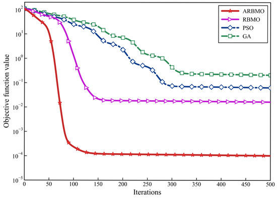
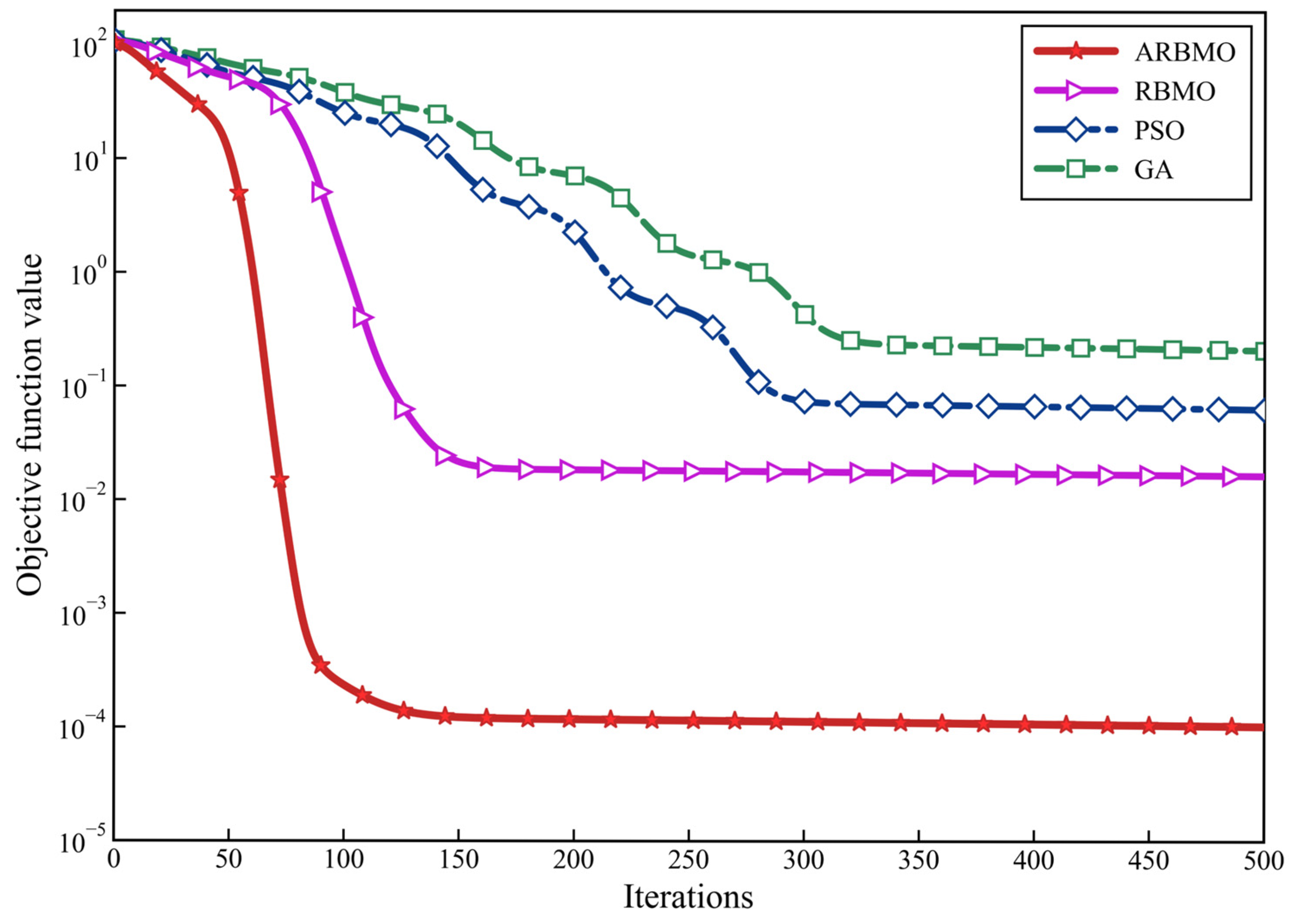
To verify the optimization performance of the proposed ARBMO, a comparative experiment was conducted. The convergence characteristics of the ARBMO were compared with the standard RBMO, Particle Swarm Optimization (PSO), and a Genetic Algorithm (GA) under the same fitness function (Equation (12)). The results are shown in Figure 1.

Figure 1. Convergence curves of different optimization algorithms for AKST parameter search.

As illustrated in Figure 1, the ARBMO achieves a lower fitness value (higher energy concentration) with a faster convergence rate compared to the RBMO, PSO, and the GA. The adaptive Concentration Factor and balance factor allow the algorithm to escape local optima effectively, which is a common limitation for PSO and GAs in high-dimensional parameter spaces. This demonstrates that the ARBMO provides a more robust and efficient solution for optimizing AKST window parameters.

To further verify the effectiveness of the ARBMO in practical signal processing, this paper conducted experimental analysis using typical PQD signals. In the experiment, the fundamental frequency $f_0$ of the PQD signal was 50 Hz, and the sampling frequency $f_s$ was set to 3200 Hz. To analyze multiple PQDs more reliably, reference [21] was used to sample the PQD signal over 10 periods, with a sampling point N of 640 and a sampling time of 0.2 s. In addition, other sampling periods were also applicable.

2.3. Time–Frequency Analysis of PQD Based on AKST

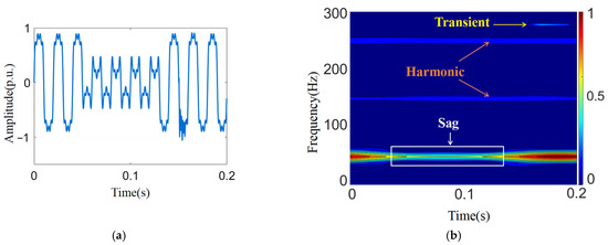
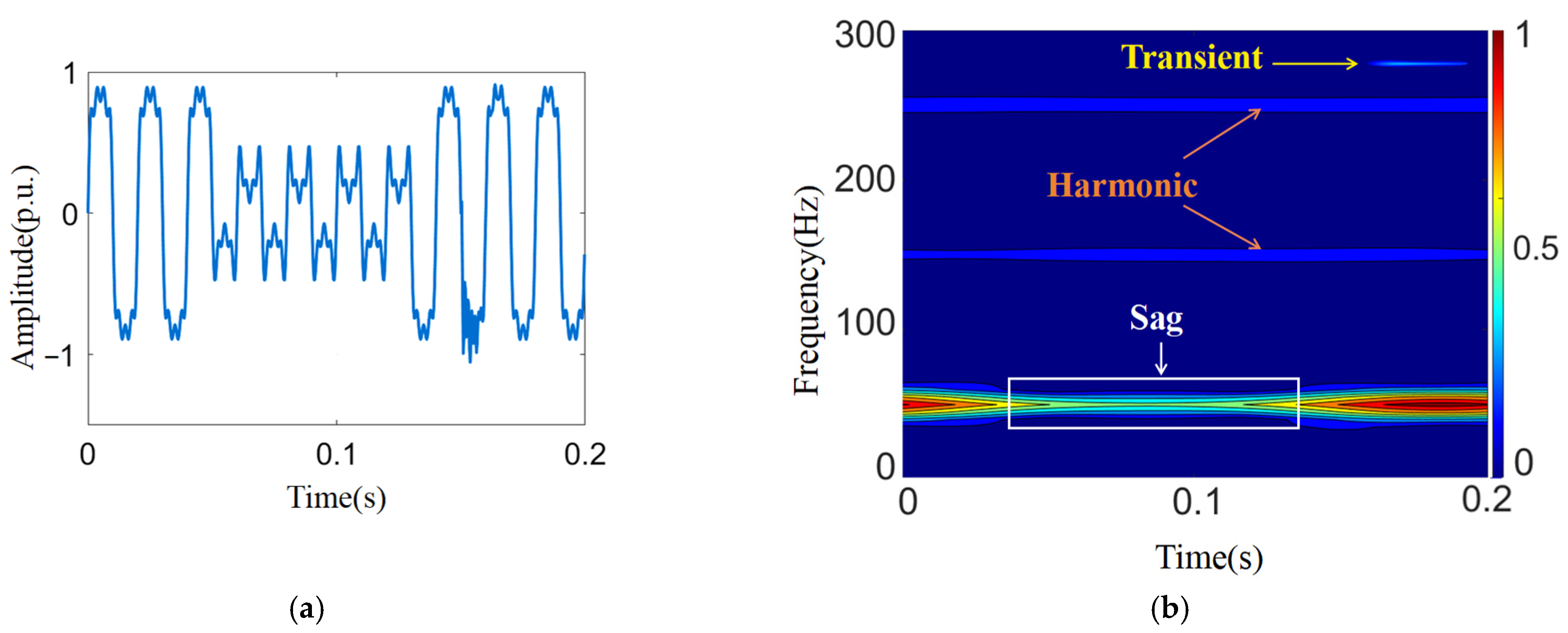
To verify the time–frequency performance of the proposed AKST using the parameters optimized by the ARBMO, PQDs with time-domain and frequency-domain interference were superimposed. This composite disturbance consists of voltage dips, harmonics, and oscillatory transients, randomly generated within 0.2 s. The disturbance signal and time–frequency analysis results are shown in Figure 2a and Figure 2b, respectively.

Figure 2. AKST time–frequency analysis results of PQD with voltage dips, harmonics, and oscillation transients. (a) Input signal; (b) time–frequency amplitude matrix based on AKST.

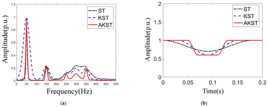
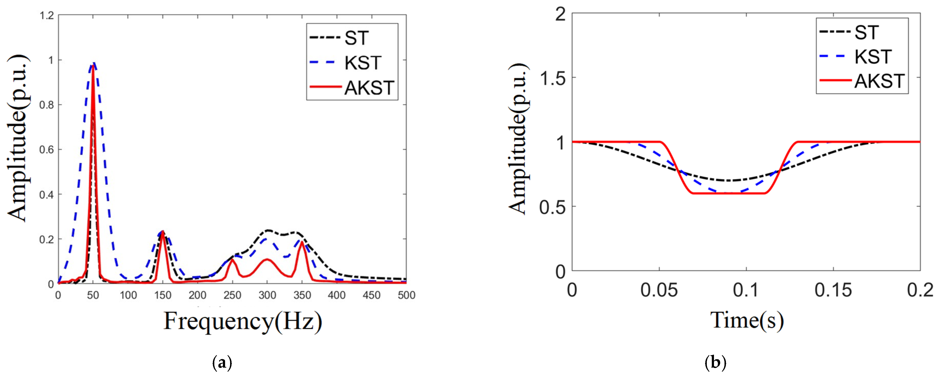
In addition, in order to reduce the computational complexity of AKST, only the key frequency point and its two nearby frequency points were considered [6]. The key frequencies included fundamental frequency and harmonic frequency. From Figure 2, it can be seen that AKST can accurately detect multiple pieces of interference information. To verify the time–frequency resolution of AKST in this article, the latest ST [20] and KST [21] were selected for comparison from both time-domain and frequency-domain perspectives, as shown in Figure 3.

Figure 3. Comparison results of time–frequency performance. (a) Amplitude curve of fundamental frequency; (b) envelope curve of frequency–amplitude.

From Figure 3, it can be seen that these three algorithms can detect voltage dips, harmonics, and oscillatory transients, demonstrating their effectiveness for PQD analysis. Compared with ST and KST, AKST in Figure 3a has a shorter time interval and higher time resolution for detecting voltage dips. In addition, from the frequency envelope curve in Figure 3b, it can be seen that AKST has a higher energy concentration and frequency resolution at the fundamental frequency. The value of AKST is 90.36, and the corresponding values of ST and KST are 80.31 and 88.45, respectively. The energy of KST is more concentrated than that of ST, which proves that Kaiser windows have a higher energy concentration than Gaussian windows. AKST is superior to KST, indicating that the control function can improve the energy concentration performance of KST. The optimal values for AKST, ST, and KST are 1.1, 0.6, and 0.2, respectively.

3. Multimodal Feature Fusion Strategy

To improve the recognition stability of PQDs under composite disturbances and noise backgrounds, this paper further introduces time-domain and frequency-domain modal representation forms. These are based on the AKST time–frequency modal representation and are used to characterize the differential features of PQDs. The article constructs three modal inputs: EMD, STFT, and AKST. A three-branch structure is used for feature extraction. The fusion layer then aligns and aggregates features across modalities to form a unified representation for subsequent classification and discrimination.

3.1. Multimodal Feature Construction and Convolutional Feature Encoding

Let the sampled PQD discrete signal be A. To characterize PQD characteristics from different modal perspectives, this paper constructs three types of modal inputs:

(1)

Time-domain mode (EMD): Perform empirical mode decomposition on X(n) to obtain several IMF components and construct the time-domain input x_EMD based on this.

(2)

Frequency-domain mode (STFT): Perform short-time Fourier transform to obtain local spectral representation and construct frequency-domain input x_STFT.

(3)

Time–Frequency Mode (AKST): Obtain the time–frequency amplitude matrix |AKS(m,n)| from the improved AKST and construct the time–frequency domain input x_AKST.

To obtain high-level representations for fusion modeling, this paper performs convolutional feature encoding across three modal inputs. Assuming the $l$-th convolutional layer and the $j$-th output channel, the convolution mapping forms for the three modal inputs are defined as follows:

$$\left\{\begin{array}{cc}{Z}_{l,j}^{EMD}& =f\left({\displaystyle {\displaystyle \sum }_{i\in M_j}}{Z}_{l-1,i}^{EMD}\ast k_{l,ij}^{EMD}+b_{l,j}^{EMD}\right)\\ Z_{l,j}^{STFT}& =f\left({\displaystyle {\displaystyle \sum }_{i\in M_j}}{Z}_{l-1,i}^{STFT}\ast k_{l,ij}^{STFT}+b_{l,j}^{STFT}\right)\\ Z_{l,j}^{AKST}& =f\left({\displaystyle {\displaystyle \sum }_{i\in M_j}}{Z}_{l-1,i}^{AKST}\ast k_{l,ij}^{AKST}+b_{l,j}^{AKST}\right)\end{array}\right.$$

(15)

where $Z_{l-1,i}^{(·)}$ is the $i$-th input channel feature of the previous layer; $\ast$ is the convolution operation; $k_{l,ij}^{(·)}$ and $b_{l,i}^{(·)}$ are the convolution kernel and bias, respectively; $M_j$ is the set of input channels connected to the output channel $j$; and $f(·)$ is the ReLU activation function.

Equation (15) is used to uniformly describe the convolutional encoding process of EMD, STFT, and AKST modal features. For the convenience of subsequent fusion modeling, the high-level features obtained by encoding the three types of modalities are respectively referred to as

$$\left\{\begin{array}{l}{Z}_{EMD}={\mathrm{\Phi }}_{EMD}\left(X_{EMD}\right)\hfill \\ Z_{STFT}={\mathrm{\Phi }}_{STFT}\left(X_{STFT}\right)\hfill \\ Z_{AKST}={\mathrm{\Phi }}_{AKST}\left(X_{AKST}\right)\hfill \end{array}\right.$$

(16)

where ${\mathrm{\Phi }}_{EMD}(·)$, ${\mathrm{\Phi }}_{EMD}(·)$, and ${\mathrm{\Phi }}_{AKST}(·)$ are the feature maps of three branches. Among them, each branch of $X(n)$ adopts Resblock as the convolutional feature extraction unit in reference [8] to achieve the branch feature mapping process described in Equations (15) and (16).

3.2. Fusion Layer Model and Weighted Fusion Strategy

The fusion layer aggregates features encoded from three modalities into a unified representation. Due to differences in the number of channels or vector dimensions across different modal features, it is necessary to ensure that the features participating in the fusion are consistent in the fusion dimension before fusion. Therefore, this article introduces alignment maps ${\mathcal{A}}_{EMD}(·)$, ${\mathcal{A}}_{STFT}(·)$, and ${\mathcal{A}}_{AKST}(·)$ to obtain the aligned branch features:

$$\left\{\begin{array}{c}{\tilde{Z}}_{EMD}={\mathcal{A}}_{EMD}\left(Z_{EMD}\right)\\ {\tilde{Z}}_{STFT}={\mathcal{A}}_{STFT}\left(Z_{STFT}\right)\\ {\tilde{Z}}_{AKST}={\mathcal{A}}_{AKST}\left(Z_{AKST}\right)\end{array}\right.$$

(17)

Alignment mapping can be achieved through linear projection, ensuring that the three types of features satisfy the same size constraints in the fusion dimension. In terms of operator definition in the fusion layer, the same layer modal features are added and aggregated, and the fusion features are obtained through nonlinear activation, defined as

$$F_r=f\left(Z_{l,j}^{EMD}+Z_{l,j}^{STFT}+Z_{l,j}^{AKST}\right)$$

(18)

where $F_r$ is the output feature of the $r$-th fusion layer and $Z_{l,j}^{EMD}$, $Z_{l,j}^{STFT}$, and $Z_{l,j}^{AKST}$ are the modal feature mapping results of the corresponding layers.

Equation (18) characterizes the process of feature aggregation within the same layer. On this basis, this article adopts a weighted fusion strategy to aggregate the three modal features and obtain the final fused feature representation:

$$\begin{array}{c}F={\alpha }_1{\tilde{Z}}_{EMD}+{\alpha }_2{\tilde{Z}}_{STFT}+{\alpha }_3{\tilde{Z}}_{AKST}\\ {\alpha }_i\ge 0,{\displaystyle \sum }_{i=1}^3{\alpha }_i=1\end{array}$$

(19)

where ${\alpha }_1$, ${\alpha }_2$ and ${\alpha }_3$ are three mode fusion weights.

To avoid weight dependence on empirical settings, this paper sets the fusion weights as learnable parameters and uses a Softmax form to ensure their non-negativity and normalization constraints:

$${\alpha }_i={\displaystyle \frac{\exp \left({\beta }_i\right)}{{{\displaystyle \sum }}_{j=1}^3\exp \left({\beta }_j\right)}},i=1,2,3$$

(20)

where ${\beta }_i$ is an unconstrained parameter that is jointly optimized with network parameters during the training process.

The ${\alpha }_1$, ${\alpha }_2$, and ${\alpha }_3$ obtained after training convergence remain unchanged during the inference phase. The final fusion feature $F_c$ is used as the input for the classifier to distinguish the type of PQD.

4. Multimodal Feature Fusion Classification Framework MFNet

After completing multimodal feature extraction and fusion, the fully connected $F_c$-layer outputs are fed into the SVM classifier for disturbance type discrimination. For the R training samples, the mathematical model is

$$\min \varphi (e)={\displaystyle \frac{1}{2}}\parallel e{\parallel }^2+c{\displaystyle \sum }_{\theta =1}^R{\zeta }_{\theta }$$

(21)

$$s.t.y_{\theta }\left(e{x}_{\theta }+\lambda \right)⩾1-{\zeta }_{\theta },\theta =1,2,\dots ,N$$

(22)

where $e$ is the normal vector of the hyperplane, $c$ is the penalty factor, ${\zeta }_{\theta }$ is the relaxation variable, $x_{\theta }$ is the training sample, and $y_{\theta }$ is the sample category. $\lambda$ is the deviation. Using the duality theorem and the Lagrange function, we obtain

$$\max L(\mu )={\displaystyle \sum }_{\theta =1}^R{\mu }_{\theta }-{\displaystyle \frac{1}{2}}{\displaystyle \sum }_{\theta ,o=1}^N{y}_{\theta }{y}_o{\mu }_{\theta }{\mu }_{o}M\left(x_{\theta },x_o\right)$$

(23)

$$s.t.\left\{\begin{array}{l}{\displaystyle \sum _{\theta =1}^N{\mu }_{\theta }}{y}_{\theta }=0\hfill \\ 0⩽{\mu }_{\theta }⩽C\hfill \end{array}\right.$$

(24)

where $\mu$ is the Lagrange multiplier; $\theta ,o$ is the sample, $\theta ,o=1,2,\dots$; and $M$ is the kernel function.

$M$ uses a Gaussian kernel function, expressed as

$$M\left(x_i,x_j\right)=\exp \left({\displaystyle \frac{-\parallel x_i-x_j{\parallel }^2}{{\delta }^2}}\right)$$

(25)

where $\delta$ is the kernel function parameter.

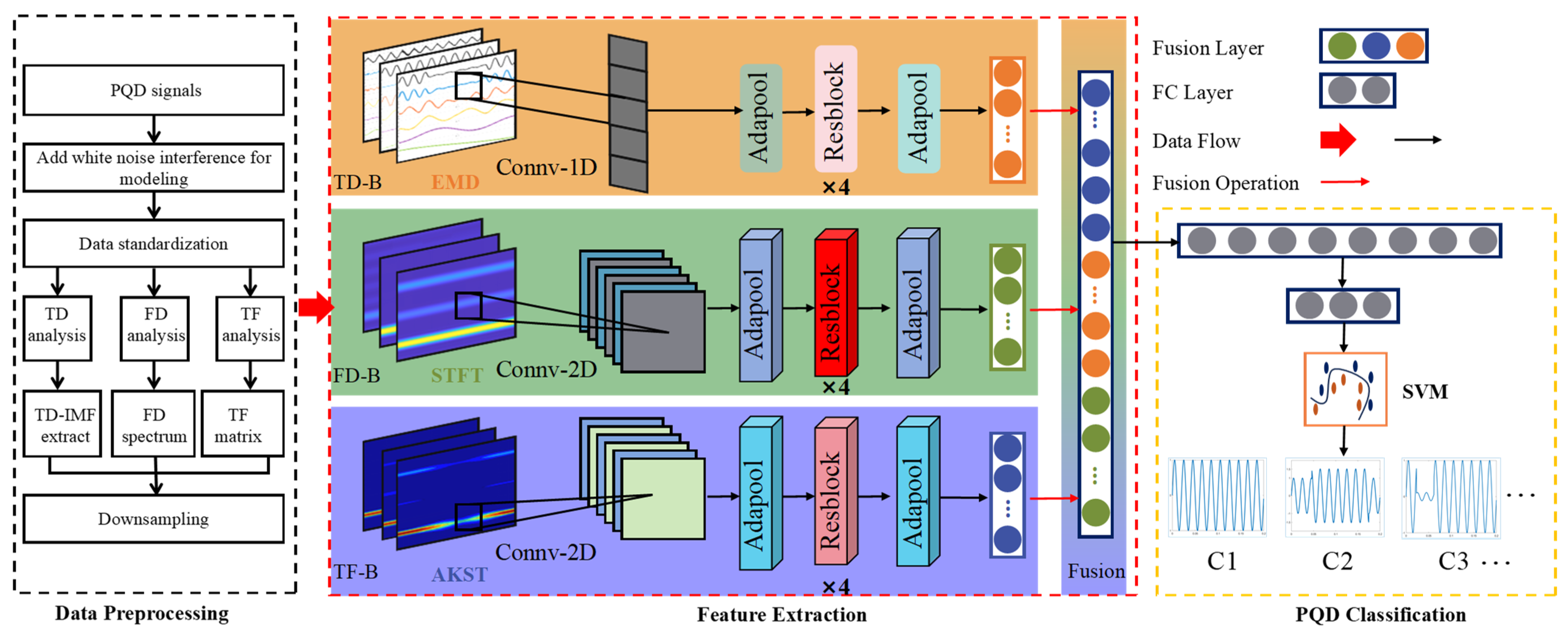
On the basis of PQD feature construction and the multimodal feature fusion strategy, this paper proposes the automatic classification method MFNet for PQDs. The specific structural diagram is shown in Figure 4.

Figure 4. PQD classification method based on MFNet.

Figure 4 shows that we can summarize the MFNet implementation process as follows:

(1)

Multimodal feature construction: Represent PQD signals in multiple modalities. Use EMD to construct time-domain modal features. Apply STFT for frequency-domain modal features. Use AKST to construct high-resolution time–frequency modal features.

(2)

Feature learning and fusion modeling: Input the three modal features into the corresponding branches of the MFNet for feature learning and extraction. At the fusion layer, align and aggregate modal features to form a unified high-level feature representation.

(3)

Classification output and training method: Input the fused high-level features into the classifier to output perturbation categories. During the training phase, a data-driven approach jointly learns network parameters and fuses weights, enabling end-to-end optimization.

The PQD recognition process is fully automated and does not require expert experience for feature intervention or screening. Multiple sets of experiments were designed to comprehensively evaluate and analyze the proposed MFNet classification method.

5. Experiment and Analysis

5.1. PQD Dataset

According to the IEEE-1159 standard [30] and reference [8], 30 types of PQDs were tested, including 9 single-PQD signals and 21 PQD signals, to verify the robustness of the MFNet. Table 2 lists all 30 PQD types.

Table 2. Thirty types of PQD signals.

Class	PQ Disturbance	Class	PQ Disturbance	Class	PQ Disturbance
C1	Normal	C11	Sag + Harmonics	C21	Transient + Harmonics + Sag
C2	Sag	C12	Swell + Harmonics	C22	Transient + Harmonics + Swell
C3	Swell	C13	Interrupt + Harmonics	C23	Transient + Harmonics + Interrupt
C4	Interrupt	C14	Transient + Harmonics	C24	Transient + Harmonics + Flicker
C5	Harmonics	C15	Flicker + Harmonics	C25	Flicker + Harmonics + Interrupt
C6	Transient	C16	Sag + Transient	C26	Flicker + Harmonics + Sag
C7	Flicker	C17	Swell + Transient	C27	Flicker + Harmonics + Swell
C8	Notch	C18	Spike + Transient	C28	Spike + Harmonics + Sag
C9	Spike	C19	Notch + Transient	C29	Spike + Harmonics + Interrupt
C10	Spike + Harmonics	C20	Flicker + Sag	C30	Spike + Harmonics + Swell

The PQD signals were randomly generated using MATLAB R2023b with a fundamental frequency of 50 Hz and a sampling frequency of 3.2 kHz. Each signal segment contained 640 sampling points (0.2 s duration). To evaluate the model’s robustness under extreme conditions, Gaussian white noise was added to the signals at signal-to-noise ratios (SNRs) of 20 dB, 30 dB, and 40 dB. For each of the 30 categories, 3000 samples were generated, resulting in a total dataset of 90,000 samples. The dataset was divided into training, validation, and testing sets according to a ratio of 6:2:2 (1800 samples for training, 600 for validation, and 600 for testing per class).

5.2. Performance Metrics and Parameter Settings

To provide a comprehensive evaluation of the classification performance, Precision, Recall, and F1-score were employed as the primary metrics. These indicators are defined as follows:

$$Precision={\displaystyle \frac{TP}{TP+FP}}$$

(26)

$$Recall={\displaystyle \frac{TP}{TP+FN}}$$

(27)

$$F1-score=2\times {\displaystyle \frac{ Precision\times Recall}{ Precision+Recall}}$$

(28)

where TP, FP, and FN represent True Positives, False Positives, and False Negatives, respectively.

The detailed structural parameters of the MFNet branches are summarized in Table 3. To ensure that features from different modalities (1D and 2D) can be fused, an Adaptive Pooling layer was employed at the end of each branch to align the feature dimensions.

Table 3. Detailed structural parameters of the three-branch MFNet.

Branch	Layer	Type	Kernel Size	Stride	Output Dimension
Input	–	–	–	–	2D: 224 × 224 × 3/1D: 640 × 1
EMD (1D)	Layer 1	Conv1D + ReLU	7	2	320 × 64
	Layer 2	Conv1D + ReLU	5	2	160 × 128
	Layer 3	Conv1D + ReLU	3	2	80 × 256
	Layer 4	Conv1D + ReLU	3	2	40 × 512
	GAP	Adaptive Pooling	–	–	512 × 1
STFT (2D)	Layer 1	Conv2D + ReLU	7 × 7	2	112 × 112 × 64
	Layer 2	Conv2D + ReLU	5 × 5	2	56 × 56 × 128
	Layer 3	Conv2D + ReLU	3 × 3	2	28 × 28 × 256
	Layer 4	Conv2D + ReLU	3 × 3	2	14 × 14 × 512
	GAP	Adaptive Pooling	–	–	512 × 1
AKST (2D)	Layer 1	Conv2D + ReLU	7 × 7	2	112 × 112 × 64
	Layer 2	Conv2D + ReLU	5 × 5	2	56 × 56 × 128
	Layer 3	Conv2D + ReLU	3 × 3	2	28 × 28 × 256
	Layer 4	Conv2D + ReLU	3 × 3	2	14 × 14 × 512
	GAP	Adaptive Pooling	–	–	512 × 1
Fusion	Weighted	Softmax Weight	–	–	512 × 1 (Fused Vector)

As shown in Table 3, the Adaptive Pooling layer ensures that each branch outputs a 512-dimensional vector regardless of the input modality. The final Fully Connected (FC) layer has a parameter matrix of 512 × 30, corresponding to the 30 PQD categories.

Training Settings: The model was trained using the Stochastic Gradient Descent (SGD) optimizer with a momentum of 0.9. The initial learning rate was 0.001, the batch size was 32, and the training process lasted for 100 epochs.

Environment: The MFNet was implemented in PyTorch 1.10.0. The hardware environment consisted of an Intel^® Xeon^® Silver 4214R CPU @ 2.40 GHz and an NVIDIA GeForce RTX 4090 GPU.

5.3. AKST’s Experimental Results

To evaluate the performance of the proposed MFNet in identifying PQD events, the trained model was assessed on the test set under various noise environments. The overall classification results, including Precision, Recall, and F1-score, are summarized in Table 4.

Table 4. Classification results of the MFNet model under different SNR levels.

Noise Level	Precision (%)	Recall (%)	F1-Score (%)
Clean	99.81	99.82	99.81
20 dB	99.50	99.52	99.51
30 dB	99.59	99.61	99.61
40 dB	99.63	99.66	99.65

As shown in Table 4, in the ideal noise-free environment, the F1-score of the MFNet reaches 99.81%. Even under the challenging condition of a 20 dB SNR, the Precision, Recall, and F1-score remain significantly high, all exceeding 99.50%. Compared to the noise-free case, the performance drop at 20 dB is minimal (less than 0.4%), which demonstrates that the MFNet exhibits exceptional classification performance across various SNR conditions and possesses superior robustness against strong background noise.

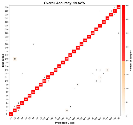
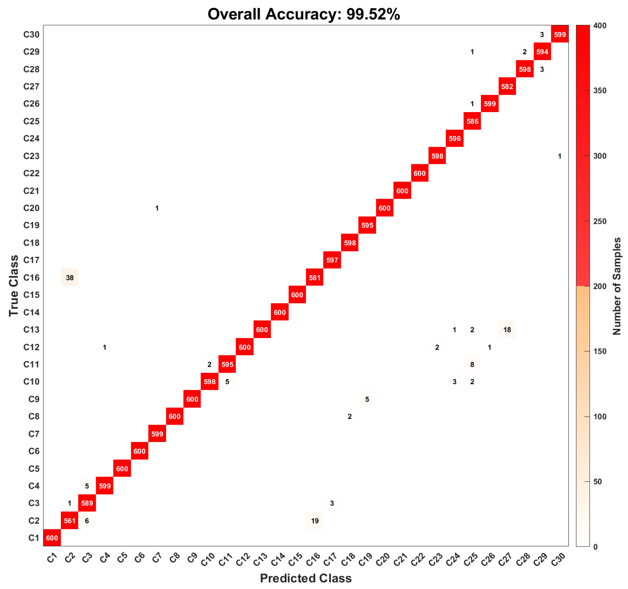
To further provide a detailed assessment of the model’s performance across all 30 PQD categories, the confusion matrix at the 20 dB noise level is illustrated in Figure 5. The confusion matrix provides a visual representation of the actual versus predicted classifications, highlighting the model’s ability to distinguish between similar and composite disturbances.

Figure 5. Confusion matrix of the MFNet for 30 types of PQDs at a 20 dB SNR.

As illustrated in Figure 5, the MFNet achieves near-perfect recognition for most single disturbances (C1–C9). For complex composite disturbances (C10–C30), such as C21 (Swell + Harmonics + Transient) and C29 (Sag + Harmonics + Spike), the model still maintains extremely high accuracy with negligible misclassification. This precision is attributed to the multimodal feature fusion strategy, which effectively integrates temporal mutations from EMD, spectral structures from STFT, and high-resolution time–frequency features from AKST. The results confirm that the MFNet can reliably capture the subtle differences between overlapping disturbance features even in high-noise environments.

5.4. Comparative Analysis of Different Time–Frequency Methods

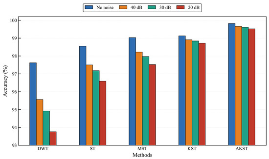
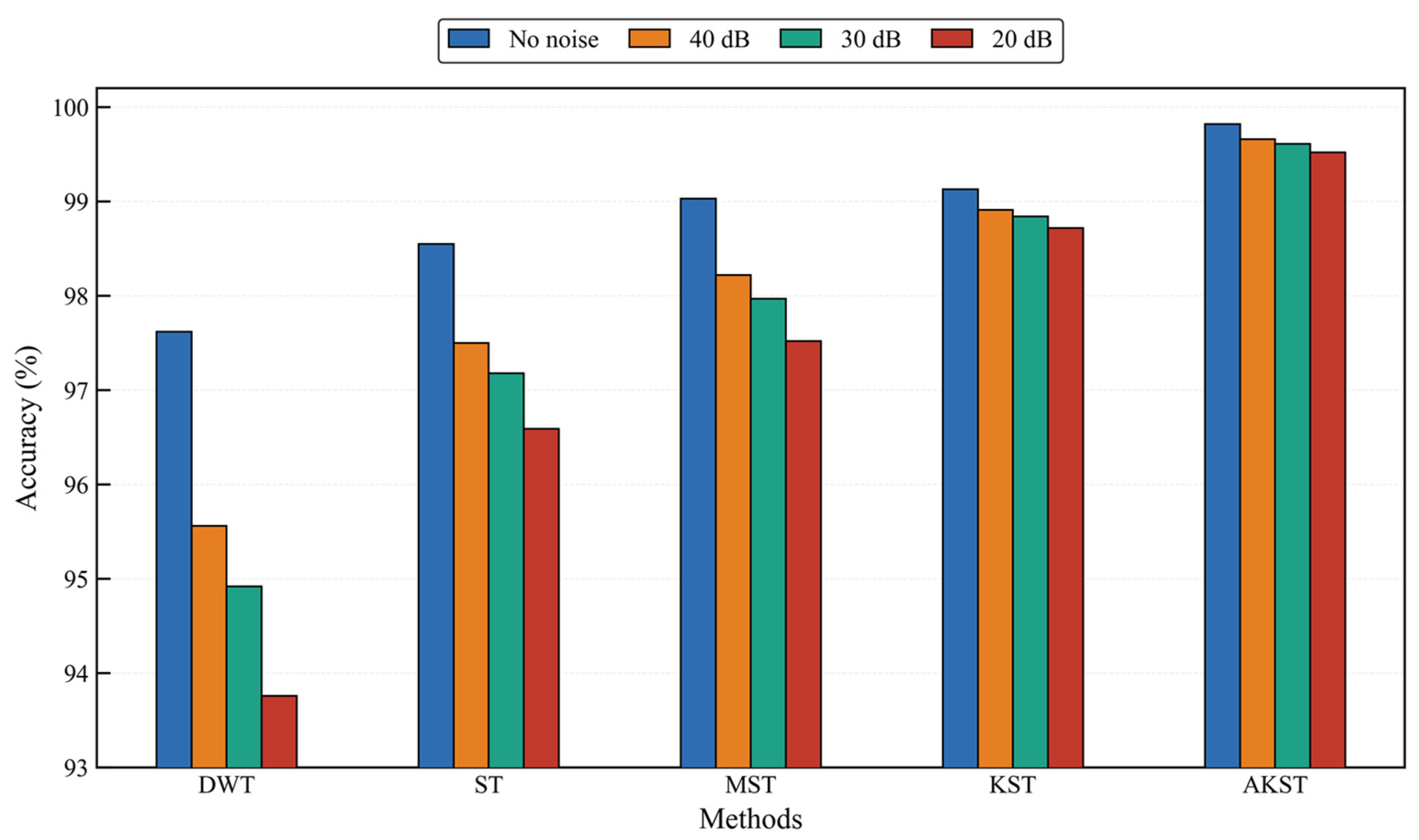
The feature information of time–frequency analysis directly affects the classification accuracy of PQDs. To verify the effectiveness of the proposed AKST, this paper compared DWT [15], ST [5], MST [16], and KST [19]. To ensure that only the time–frequency method is the variable, each method (DWT, ST, MST, KST, and AKST) was integrated separately into the same branch, while keeping the input and network structures of the time-domain and frequency-domain branches unchanged. To provide a more intuitive visualization of the performance differences across various SNR levels, the experimental results are presented as a bar chart in Figure 6.

Figure 6. Accuracy comparison of different time–frequency methods under various noise levels.

As illustrated in Figure 6, it is evident that the classification accuracy of all methods decreases as the noise level increases. However, the degree of sensitivity to noise varies significantly among the methods. In terms of accuracy, the performance degradation of DWT is more pronounced when noise is added compared to other methods; for example, its accuracy drops from 97.62% in a clean environment to 93.76% at 20 dB, indicating that DWT-based features are highly susceptible to noise interference.

In contrast, the methods based on the S-transform (ST, MST, KST, and AKST) exhibit better stability. Notably, KST and AKST are superior to other time–frequency methods, with AKST achieving the highest accuracy of 99.52% even at a 20 dB SNR. The performance of KST is not as good as that of AKST, which directly validates that the proposed ARBMO-driven adaptive control function significantly improves the transform’s adaptability to different PQD types. This result further demonstrates that AKST possesses superior feature extraction capability and exceptional robustness, providing the most stable discriminative information for the multimodal fusion network.

5.5. Ablation Experiment and Complexity Analysis

To quantify the contribution of each modal branch and evaluate the computational efficiency of the proposed framework, extensive ablation experiments were conducted. These tests were performed under a 20 dB SNR environment using the training configurations specified in Section 5.2. To ensure a fair comparison, the underlying neural network backbone (i.e., the number of layers and channels) was kept constant across all multi-branch configurations. The performance, parameter size, and total inference time (including signal pre-processing and network forward pass) are summarized in Table 5.

Table 5. Performance and complexity comparison of different model configurations (at 20 dB SNR).

Model Configuration	Parameters (M)	Inference Time (ms)	F1-Score (%)
TD only (EMD)	1.25	0.35	89.44
FD only (STFT)	4.82	0.62	86.11
TF only (AKST)	4.82	0.65	94.00
EMD + STFT	6.07	0.88	89.33
STFT + AKST	9.64	1.15	95.89
EMD + AKST	6.07	0.92	96.78
HHT + STFT + AKST	10.89	1.35	94.78
EMD + SS + AKST	10.89	1.32	95.00
HHT + SS + AKST	10.89	1.38	93.11
MFNet (Full)	10.89	1.32	97.56

Based on the results in Table 5, the following observations can be made regarding the model complexity and fusion gain:

Effectiveness of Multimodal Fusion: Single-branch configurations exhibit limited recognition capabilities, with the TD-only and FD-only models achieving F1-scores of only 89.44% and 86.11%, respectively. By integrating all three modalities, the MFNet achieves a peak F1-score of 97.56%. This significant improvement validates that the fusion of time, frequency, and time–frequency domains effectively mitigates the “feature sparsity” inherent in single modalities, capturing complementary information essential for identifying complex PQDs.

Contribution of the AKST Branch: Among the single-branch models, the TF-only (AKST) configuration demonstrates the highest accuracy (94.00%) with a parameter size of 95.78 M. The relatively higher inference time (118.65 ms) for this branch is attributed to the computational complexity of the ARBMO-driven adaptive window optimization; however, this branch provides the most discriminative representation for non-stationary disturbances.

Compatibility of Feature Extraction Methods: To verify the selection of EMD and STFT, they were replaced with alternative methods such as Hilbert–Huang Transform (HHT) and Spectral Subtraction (SS). Although these configurations share the same parameter size (226.80 M) due to the consistent network backbone, their F1-scores are lower than that of the proposed MFNet. Furthermore, configurations involving HHT exhibit higher total latency (up to 198.75 ms), indicating that the combination of EMD and STFT provides a superior balance between robustness and computational efficiency.

Real-time Feasibility Analysis: The full MFNet architecture contains 226.80 million parameters, reflecting its high-capacity feature extraction capability. On the NVIDIA GeForce RTX 4090 platform, the total inference time per sample is 188.42 ms. Given that the sampling window for PQD signals is 200 ms, the MFNet operates within the real-time processing constraint. This demonstrates that the proposed method achieves an optimal trade-off between high-precision classification and operational latency, making it suitable for practical power quality monitoring in modern grids.

5.6. Comparison of Different Detection Methods

To comprehensively evaluate the performance of the MFNet framework, this section compares the proposed model with several mainstream methods, specifically focusing on the architectures suggested in the recent literature, such as Wavelet-CNN, S-transform-SVM, and hybrid CNN-LSTM models. The comparison results are categorized into manual and automatic feature extraction methods, all assessed under a 20 dB noise environment as summarized in Table 6.

Table 6. Performance comparison with other methods.

Framework	Number of PQDS	Feature Extraction Method	SNR (dB)	Accuracy (%)
ACMP + GOA-SVM [22]	27	Manual	20	97.13
WT-SFA + LSTM [11]	16	Manual	20	97.37
IPSO-CNN [13]	16	Manual	20	98.17
S-transform + SVM [31]	16	Manual	20	97.45
RP + KD-MNV3 [20]	27	Automatic	20	96.76
CTranCBA [25]	23	Automatic	20	98.75
Wavelet + CNN [32]	20	Automatic	20	97.80
Hybrid CNN-LSTM [33]	14	Automatic	20	98.12
MFNet	30	Automatic	20	99.52

As illustrated in Table 6, the proposed MFNet exhibits clear advantages over existing benchmarks.

Firstly, in terms of recognition performance, the results indicate that the PQD recognition method based on automatic feature extraction generally outperforms manual extraction methods in terms of average accuracy. This suggests that automatic extraction effectively reduces information loss and improves recognition ceilings. Notably, the MFNet achieves the highest accuracy of 99.52% at a 20 dB SNR, outperforming hybrid architectures such as CNN-LSTM [33] and CTranCBA [25].

Comprehensive Disturbance Coverage: While most comparative methods focus on a limited set of 14 to 27 PQD types, the MFNet successfully identifies 30 types, including highly complex composite disturbances. This broader coverage highlights the framework’s superior generalization and its capacity to meet the requirements of complex modern power grids.

Robustness to Strong Noise: Even under the challenging 20 dB noise condition, the MFNet maintains exceptional stability. This stability results from the multimodal fusion strategy, which compensates for the “feature sparsity” of a single modality by integrating complementary information from the time, frequency, and time–frequency domains. Meanwhile, the ARBMO-optimized AKST branch further ensures that the input features are more discriminative than standard transforms used in [31,32].

5.7. Experimental Verification Analysis

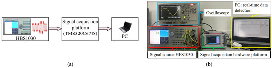
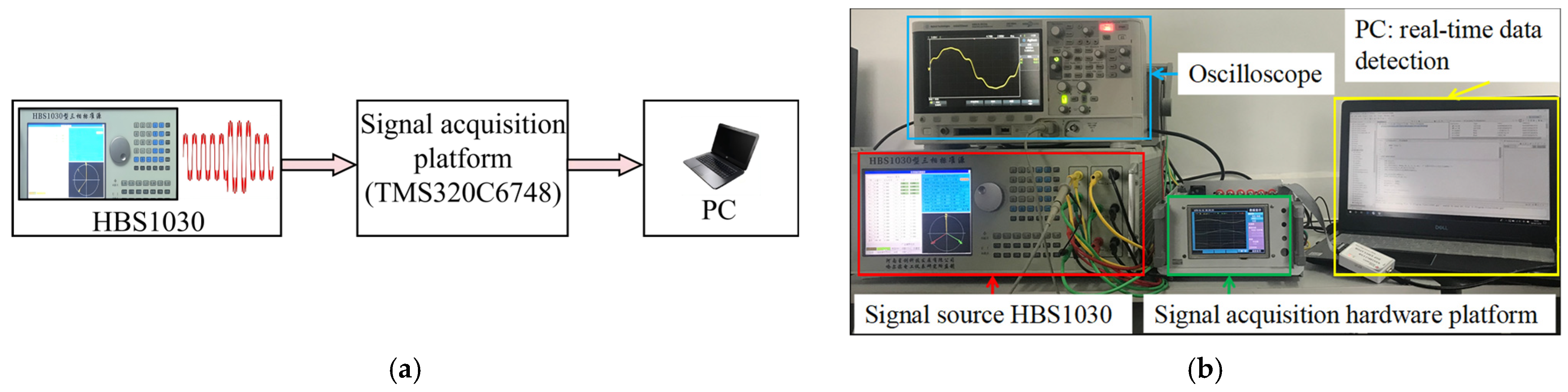
To bridge the gap between theoretical simulation and practical engineering, a hardware platform for PQD detection was designed, based on [5,8], to verify the real-time performance and reliability of the MFNet model in a physical environment. While simulation enables comprehensive testing of all 30 PQD types under controlled noise, the hardware experiment focuses on validating the model’s feasibility using real-world acquisition circuits and processors. The hardware platform is shown in Figure 7, including the experimental signal standard source HBS1030, signal acquisition platform, and signal analysis PC.

Figure 7. PQD sampling hardware platform. (a) PQD signal sampling principle diagram; (b) hardware platform.

Due to the limitations of the HBS1030 output function, five types of PQDs were tested: C1, C2, C3, C5, and C9. After preheating, HBS1030 randomly generated different PQDs. The data acquisition platform used a 16-bit ADS8556 analog-to-digital converter (Texas Instruments, Dallas, TX, USA) and a 32-bit floating-point TMS320C6748 processor (Texas Instruments, Dallas, TX, USA), with a clock frequency of 375 MHz and a sampling frequency of 5 kHz. The required sampling frequency was obtained through downsampling, the signal was collected using a voltage transformer. After completing signal sampling, the data was transmitted in real time to the computer via the DSP’s serial interface. For each PQD type, 70 samples were tested to evaluate the classification performance of the proposed MFNet under experimental conditions. The average test time per sample, encompassing data acquisition, AKST/EMD pre-processing, and model inference, was recorded to validate real-time feasibility. The experimental results are summarized in Table 7.

Table 7. Performance under experimental signals.

Class	Accuracy (%)	Average Accuracy (%)	Average Test Time (ms)
C1	100	98.86	184
C2	97.14		189
C3	98.57		190
C5	100		188
C9	98.57		189

As shown in Table 7, the proposed method achieves an average accuracy of 98.86% on experimental signals, which is highly consistent with the simulation results. The average total test time is approximately 188 ms per sample. Considering that the analysis window length for 10 cycles at a 50 Hz fundamental frequency is 200 ms, the total processing time (including complex adaptive transformations and multimodal fusion inference) remains within the real-time operational limit. The results indicate that the proposed study can meet the requirements of real-time classification and verify its practicality.

6. Conclusions

To address the limitations of traditional methods in identifying complex power quality disturbances, this paper proposes a recognition framework based on AKST and an MFNet. The main conclusions are as follows:

(1)

The proposed AKST, optimized by the ARBMO algorithm, adaptively adjusts window parameters to enhance energy concentration and time–frequency resolution, providing robust features for complex PQDs.

(2)

The three-branch MFNet effectively integrates time, frequency, and time–frequency information, achieving an average accuracy of 99.52% at a 20 dB SNR and mitigating the information loss inherent in single-modal methods.

(3)

Hardware experiments confirm the framework’s real-time feasibility, with a total processing time of 188.42 ms, which remains within the 200 ms operational limit for practical power systems.

However, the study has certain limitations: the model’s performance may be sensitive to extreme noise (below 10 dB), and its relatively large parameter size (226.80 M) poses challenges for deployment on resource-constrained embedded devices.

Future research will focus on model compression and lightweight architectures to facilitate edge-side deployment and enhance the model’s robustness under extreme grid conditions and communication delays.

References

- Saeed, F.; Aldera, S.; Alkhatib, M.; Al-Shamma’a, A.A.; Hussein Farh, H.M. A data-driven convolutional neural network approach for power quality disturbance signal classification (DeepPQDS-FKTNet). Mathematics 2023, 11, 4726. [Google Scholar] [CrossRef] [Scilit]
- Cai, J.; Zhang, K.; Jiang, H. Power quality disturbance classification based on parallel fusion of CNN and GRU. Energies 2023, 16, 4029. [Google Scholar] [CrossRef] [Scilit]
- Fan, P.; Bu, S.; Li, S.; Fang, S.; Zhang, C.; Ke, S. Resilience enhancement strategy for multi-microgrids with electric vehicle under extreme weather conditions. CSEE J. Power Energy Syst. 2025, early access. [Google Scholar]
- Wu, Y.; Wu, K.; Qian, C.; Wu, J.; Tang, R. Research on Power Quality Disturbance Identification by Multi-Scale Feature Fusion. Big Data Cogn. Comput. 2026, 10, 18. [Google Scholar] [CrossRef] [Scilit]
- Ma, J.; Tang, Q.; He, M.; Peretto, L.; Teng, Z. Complex PQD classification using time–frequency analysis and multiscale parallel attention residual network. IEEE Trans. Ind. Electron. 2024, 71, 9658–9667. [Google Scholar] [CrossRef] [Scilit]
- Teng, Z.S.; Liang, C.B.; Tang, Q.; Zhang, L.; Cheng, D. K–S transform and its application in time–frequency analysis of power-grid supraharmonics. J. Hunan Univ. Nat. Sci. 2024, 51, 128–136. (In Chinese) [Google Scholar] [CrossRef]
- Yin, B.Q.; Chen, Q.B.; Li, B.; Zuo, L. A novel method for identification and classification of power quality disturbances based on improved Kaiser window fast S-transform and LightGBM. Proc. CSEE 2021, 41, 8372–8384. (In Chinese) [Google Scholar] [CrossRef]
- Ma, J.; Liu, J.; Qiu, W.; Tang, Q.; Wang, Q.; Li, C.; Peretto, L.; Teng, Z. An intelligent classification framework for complex PQDs using optimized KS-transform and multiple fusion CNN. IEEE Trans. Ind. Inform. 2024, 20, 1776–1785. [Google Scholar] [CrossRef] [Scilit]
- Chen, T.; Zhao, Y.; Li, T.; Luo, P.; Hou, Y.; Li, Z. Automatic identification of power quality signal of distribution network based on HHT and RVM. In Proceedings of the 2021 China International Conference on Electricity Distribution (CICED), Shanghai, China, 7–9 April 2021. [Google Scholar] [CrossRef] [Scilit]
- Li, H.; Yi, B.; Li, Q.; Ming, J.; Zhao, Z. Evaluation of DC power quality based on empirical mode decomposition and one-dimensional convolutional neural network. IEEE Access 2020, 8, 34339–34349. [Google Scholar] [CrossRef] [Scilit]
- Cheng, Z.Y.; Jiang, S.; Hu, J.; Wang, D.S. Power quality disturbance classification based on improved PSO for optimizing the number of convolution kernels. Adv. Technol. Electr. Eng. Energy 2023, 42, 40–49. (In Chinese) [Google Scholar] [CrossRef]
- Zang, X.; Zhang, T.J.; Shao, X.Y.; Yang, S.; Chen, Z.H.; Wu, J.L. Internal mechanical fault diagnosis of transformer based on time-varying filtering EMD and SSA-LSSVM. Electr. Mach. Control Appl. 2023, 50, 49–56. (In Chinese) [Google Scholar]
- Jin, X.; Zhou, K.X.; Yu, H.Z.; Wang, S.H.; Wu, M.H. Power quality disturbance classification method based on convolutional neural network and Transformer. Sci. Technol. Eng. 2024, 24, 6726–6733. (In Chinese) [Google Scholar] [CrossRef]
- Liu, J.; Tang, Q.; Ma, J.; Liang, L.; Qiu, W. IsDenseNet: A framework for complex power quality disturbances detection. In Proceedings of the 2021 7th International Conference on Computer and Communications (ICCC), Chengdu, China, 10–13 December 2021. [Google Scholar] [CrossRef] [Scilit]
- Markovska, M.; Taskovski, D.; Kokolanski, Z.; Dimchev, V.; Velkovski, B. Real-time implementation of optimized power quality events classifier. IEEE Trans. Ind. Appl. 2020, 56, 3431–3442. [Google Scholar] [CrossRef] [Scilit]
- Liang, C.; Teng, Z.; Liu, J.; Yao, W.; Wang, L.; He, Q.; Hu, S. Improved S-transform for time-frequency analysis for power quality disturbances. IEEE Trans. Power Deliv. 2022, 37, 2942–2952. [Google Scholar] [CrossRef] [Scilit]
- Li, N.; Wang, R.Y.; Zhu, L.H. Power quality detection and identification based on empirical wavelet transform and improved S-transform. Dianqi Chuandong 2024, 54, 26–33, 72. (In Chinese) [Google Scholar] [CrossRef]
- Samal, L.; Palo, H.K.; Sahu, B.N.; Samal, D. The classification of power quality disturbances using statistical S-transform and probabilistic neural network. In Proceedings of the 2021 1st Odisha International Conference on Electrical Power Engineering, Communication and Computing Technology (ODICON), Bhubaneswar, India, 8–9 January 2021. [Google Scholar] [CrossRef] [Scilit]
- Liang, C.; Teng, Z.; Li, J.; Yao, W.; Hu, S.; Yang, Y.; He, Q. A Kaiser window-based S-transform for time-frequency analysis of power quality signals. IEEE Trans. Ind. Inform. 2022, 18, 965–975. [Google Scholar] [CrossRef] [Scilit]
- Chiam, D.H.; Lim, K.H.; Law, K.H. LSTM power quality disturbance classification with wavelets and attention mechanism. Electr. Eng. 2023, 105, 259–266. [Google Scholar] [CrossRef] [Scilit]
- Qiu, W.; Tang, Q.; Liu, J.; Teng, Z.; Yao, W. Power quality disturbance recognition using modified S transform and parallel stack sparse auto-encoder. Electr. Power Syst. Res. 2019, 174, 105876. [Google Scholar] [CrossRef] [Scilit]
- Motlagh, S.Z.; Foroud, A.A. Power quality disturbances recognition using adaptive chirp mode pursuit and grasshopper optimized support vector machines. Measurement 2021, 168, 108461. [Google Scholar] [CrossRef] [Scilit]
- Zhu, Y.; Tao, Y.W.; Li, Z.Q. Power quality disturbance identification based on S-transform and feature selection. Diangong Jishu 2023, 21, 97–100. (In Chinese) [Google Scholar] [CrossRef]
- Fu, S.; Li, K.; Huang, H.; Ma, C.; Fan, Q.; Zhu, Y. Red-billed blue magpie optimizer: A novel metaheuristic algorithm for 2D/3D UAV path planning and engineering design problems. Artif. Intell. Rev. 2024, 57, 134. [Google Scholar] [CrossRef] [Scilit]
- He, C.; Li, K.; Dong, Y.; Song, Z.; Xiao, X.; Li, B.; Li, X. Power quality composite disturbance identification based on knowledge distillation and RP-MobileNetV3. Power Syst. Prot. Control 2023, 51, 75–84. [Google Scholar] [CrossRef]
- Li, Z.Y.; Chen, Q.; Qian, B.Q.; Niu, Y.H.; Zhang, Z.W. Health diagnosis of grid-connected inverter switching devices based on Gramian angular field and parallel CNN. Electr. Power Autom. Equip. 2024, 44, 153–159. (In Chinese) [Google Scholar] [CrossRef]
- He, M.; Li, J.; Mingotti, A.; Tang, Q.; Peretto, L.; Teng, Z. Deep Fractional Multidimensional Spectrum Convolutional Neural Fusion Network for Identifying Complex Power Quality Disturbance. IEEE Trans. Instrum. Meas. 2024, 73, 9005412. [Google Scholar] [CrossRef] [Scilit]
- Cai, L.; Zhang, K.; Sun, G. Power quality disturbance identification method based on multi-domain feature fusion. In Proceedings of the IEEE 14th Conference on Industrial Electronics and Applications (ICIEA), Xi’an, China, 19–21 June 2019; p. 8833682. [Google Scholar] [CrossRef] [Scilit]
- El-Fergany, A.A.; Agwa, A.M. Red-billed blue magpie optimizer for electrical characterization of fuel cells with prioritizing estimated parameters. Technologies 2024, 12, 156. [Google Scholar] [CrossRef] [Scilit]
- IEEE Std 1159-1995; IEEE Recommended Practice for Monitoring Electric Power Quality. IEEE Power and Energy Society: New York, NY, USA, 1995; pp. 1–80.
- Ribeiro, V.M.; Santos, N.D.S.M.D.; Kapisch, E.B.; Silva, L.R.M.; Duque, C.A. Real-Time Implementation of Stockwell Transform in FPGA Platform Using Soft-Core Processor Applied to Novelty Detection in Power Quality Signals. J. Control Autom. Electr. Syst. 2024, 35, 509–521. [Google Scholar] [CrossRef] [Scilit]
- Zeng, Q.; Wang, X.; Yang, R.; Jike, N.; Peng, Y.; Wang, J.; Tian, Y.; Zhou, C.; Ruan, S.; Yan, D. Power quality disturbance classification using wavelet transform and convolutional neural network. Measurement 2021, 175, 109141. [Google Scholar] [CrossRef] [Scilit]
- Ke, N.; Shen, N.; Guo, C. A Hybrid CNN-BiLSTM Model for Power Quality Disturbances Classification. In Proceedings of the 2024 4th International Conference on New Energy and Power Engineering (ICNEPE), Xi’an, China, 13–15 December 2024; pp. 1038–1045. [Google Scholar] [CrossRef] [Scilit]
Disclaimer/Publisher’s Note: The statements, opinions and data contained in all publications are solely those of the individual author(s) and contributor(s) and not of MDPI and/or the editor(s). MDPI and/or the editor(s) disclaim responsibility for any injury to people or property resulting from any ideas, methods, instructions or products referred to in the content. |
© 2026 by the authors. Licensee MDPI, Basel, Switzerland. This article is an open access article distributed under the terms and conditions of the Creative Commons Attribution (CC BY) license.