


Abstract
Quantifying the complex spatial–temporal correlations and generating representative high-dimensional coupled scenario sets are essential for the robust planning and risk assessment of large-scale hybrid energy systems (HESs). Although numerous models have been developed for this purpose, as the number of plants scales up to hundreds, existing approaches suffer from the curse of dimensionality, often resulting in high computational burden, posterior collapse, and distributional oversmoothing. To address this gap, this paper proposes a Spatial-Clustering Conditional Variational Auto-Encoder (SC-CVAE) framework, which employs spatial clustering to decompose the high-dimensional global problem into tractable subproblems and integrates adaptive deep networks to accurately capture high-dimensional spatiotemporal complementarity. Case studies on the Yalong River energy base, featuring massive wind and solar integration, demonstrate that SC-CVAE reduces global spatial correlation error by 56% compared to the Independent Baseline, while achieving a 2.4-fold computational speedup over the monolithic Global Baseline. Crucially, by mitigating posterior collapse to alleviate oversmoothing effects inherent in high-dimensional VAEs, the proposed framework improves the capture rate of high-impact extreme events by 3.4-fold and reduces the Energy Score error by 65%. This high-fidelity reconstruction of tail characteristics provides a more reliable basis for identifying supply-deficit risks in basin-wide HESs. The proposed framework enables scalable and high-fidelity generative modeling, establishing a robust methodology for stochastic optimization and long-term security assessments in the global transition toward decarbonized power systems.
1. Introduction
In the context of the global energy transition, the deployment of large-scale Hybrid Energy Systems (HESs) incorporating wind and solar has become a primary pathway toward decarbonized power grids [1,2,3,4]. Within this framework, the high-fidelity characterization of wind and solar resource is the fundamental prerequisite for reliable capacity planning and system operation. Since renewable outputs exhibit significant stochasticity, scenario generation technologies have emerged to provide the stochastic diversity required for robust optimization [5,6]. These technologies enable system planners to test grid resilience against various uncertainty realizations, avoiding suboptimal configurations that lead to energy curtailment or supply deficits [7,8].
Scenario generation initially relied on historical sampling methods [9], such as block bootstrapping [10] and typical days clustering [11,12]. While these approaches generate scenarios by re-sampling and reorganizing historical data without requiring explicit probability assumptions, their diversity is strictly constrained by the historical records. This lack of extrapolative capability renders them insufficient for robustness design, testing the system against extreme, low-probability scenarios is essential [13].
To overcome this, researchers shifted toward parametric modeling, beginning with marginal distribution fitting—such as Weibull distributions and Beta distributions. To represent spatial–temporal interactions, multivariate methods such as Copula functions [14,15,16,17,18,19] were utilized for joint distribution modeling, while MCMC [20] was employed to sample from complex stochastic processes. While mathematically rigorous, these methods encounter the “curse of dimensionality” as dimensions expand; parameter estimation becomes numerically unstable and computationally prohibitive [16,21].
Recently, deep generative models, including Generative Adversarial Networks (GANs) [6,22,23,24] and Variational Autoencoders (VAEs) [9,25], as well as hybrid architectures, such as VAE-DCGAN [26], VAEGAN [27,28] or PG-GAN [29], have offered new paths for scenario generation. By utilizing neural networks to learn implicit distributions, these architectures aim to bypass the limitations of explicit probabilistic assumptions. However, while these models are theoretically capable of high-dimensional modeling, their practical performance is often highly sensitive to the scale of the input space. As dimensions increase, maintaining a stable balance between data reconstruction and feature learning remains a significant open challenge.
This challenge is particularly acute in HESs, where robust system planning relies heavily on generating scenarios with adequate stochastic diversity. In this physical context, such diversity is not merely random numerical variance; rather, it is defined by the model’s capacity to accurately reconstruct both the precise probabilities of extreme tail distributions and the authentic spatial correlation structures between distributed stations. However, when forced to capture the implicit joint probability distributions of hundreds of dimensions simultaneously to achieve this required diversity, these generative models are often plagued by distinct failure modes. While GANs are notoriously susceptible to mode collapse [30]—a state where the generator produces limited varieties of samples—VAEs frequently encounter posterior collapse in high-dimensional settings.
From a numerical optimization perspective, the root of posterior collapse in high-dimensional tasks lies in the numerical imbalance within the objective function. The reconstruction loss is an aggregate error computed over the entire spatial–temporal grid (number of stations × time steps), causing its magnitude to physically dominate loss function. This gradient imbalance incentivizes the model to collapse the latent space to minimize the Kullback–Leibler (KL) divergence prematurely. Consequently, this results in over-smoothed scenarios where the decoder, deprived of informative latent variables, converges to a statistical mean that fails to represent the physical variability and extreme fluctuations inherent in intermittent energy generation.
If a generative model loses this stochastic diversity, becoming over-smoothed and spatially decoupled, it fails to capture the complex spatial correlations driven by large-scale meteorological phenomena, such as cold fronts or high-pressure ridges [31]. Across a river basin, for instance, renewable energy stations often exhibit synchronous behaviors—manifesting as a simultaneous, basin-wide plunge in wind power output during a widespread winter cold front. From a practical engineering perspective, a generated scenario set is deemed physically inadequate for robust planning if it exhibits a magnitude-level degradation in capturing extreme tail events compared to historical baselines, or if it fails to preserve the physical synchronicity between adjacent sites. Relying on these smoothed and independent scenarios fosters blind optimism in system planning. Neglecting these spatial linkages inevitably leads to a significant underestimation of aggregate system volatility, masking potential operational risks, which directly exposes the grid to severe capacity underestimation and supply shortages [32].
To address the challenges between high-dimensional modeling difficulty and spatial correlation necessity, this paper proposes a systematic scenario generation framework. The main contributions are as follows:
- A Spatial-Clustering Conditional Variational Autoencoder (SC-CVAE) framework is developed to mitigate the curse of dimensionality while preserving spatial dependencies. This approach employs a physical clustering-guided mechanism—utilizing meteorological similarities—to ensure the deep learning architecture aligns with the underlying physical correlations of the multisite system. By decomposing high-dimensional global variables into localized intra-cluster subsets, the framework structurally addresses the gradient imbalance issue, effectively mitigating posterior collapse and preserving the stochastic diversity of generated scenarios.
- An adaptive network architecture is developed to adjust hidden layer dimensions according to the cluster scale, ensuring modeling consistency across varying input dimensions. To represent the distinct physical properties of wind and solar power, a differentiated composite loss function is implemented. Specifically, Mean Squared Error (MSE) is used for stochastic wind profiles, while Binary Cross-Entropy (BCE) is applied to solar power to capture its bimodal distribution and diurnal patterns.
- A dual-benchmark validation framework is established to evaluate the performance of the proposed method. Comparisons with an “Independent Baseline” verify the model’s ability to reconstruct complex spatial correlations and synchronous weather responses. Furthermore, comparisons with a “Global Baseline” demonstrate the framework’s advantages in reducing computational complexity and capturing tail characteristics of extreme events.
The remainder of this paper is organized as follows. Section 2 details the proposed SC-CVAE framework and the construction of benchmark models. Section 3 describes the case study data and evaluation metrics. Section 4 presents experimental results, validating the framework’s superiority in spatial reconstruction and computational efficiency. Finally, Section 5 concludes the paper.
2. Problem Description and Data Organization
2.1. Case Study and Data Sources
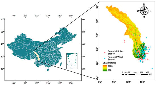
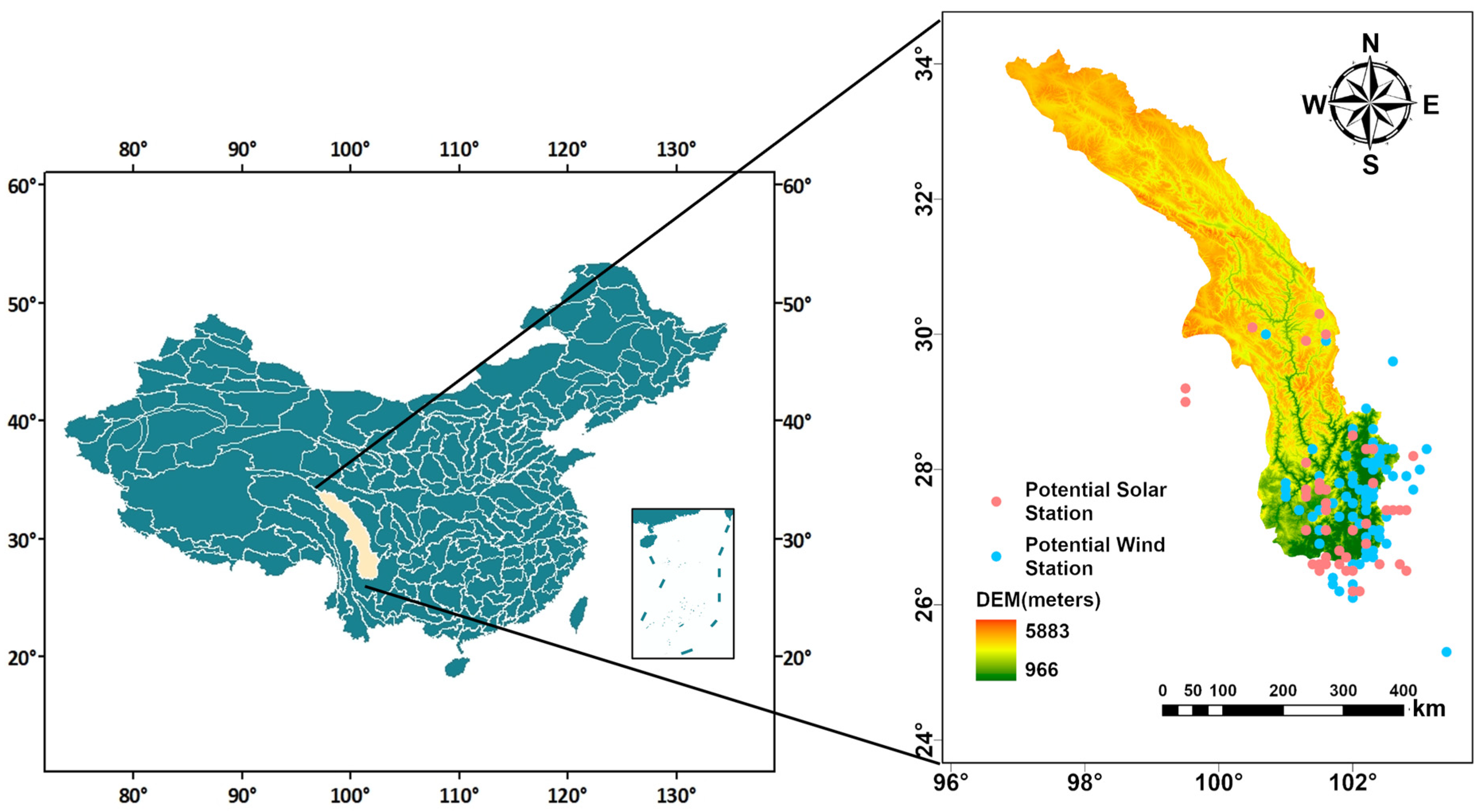
This study explores the large-scale wind and solar energy development in the Yalong River Basin, situated in southwestern China, as a case study, as shown in Figure 1. To maximize the utilization of clean energy, the basin’s managing company is accelerating the construction of wind and solar plants to increase the generation of clean energy. Based on geological surveys, the company has identified 99 potential wind power sites and 55 potential solar power sites. The maximum exploitable potential of wind and solar are 14,000 MW and 15,630 MW respectively. For meteorological inputs, we utilize the ERA5 reanalysis dataset [33] spanning from 1940 to 2022, with a temporal resolution of 1 h. These meteorological inputs are processed using the feedinlib library [34] to generate site-specific capacity factor time series.
Figure 1.
Geographically proximate candidate sites of wind and solar stations.
2.2. Data Organization
The training process begins with organizing historical power data into a structured format that the SC-CVAE can process. To preserve the spatiotemporal correlations within each cluster, we define a single daily sample as the basic processing unit. For a cluster containing stations, the long-term historical power sequence is sliced into independent daily samples. Each sample is reshaped into a 2D matrix of shape , where rows represent the 24-h time points and columns represent the spatially correlated stations. This structure ensures the simultaneous capture of intra-day temporal transitions and inter-station spatial dependencies.
To mathematically represent seasonal information within a unified training framework, each 24 h power sample is associated with a 12-dimensional one-hot encoding vector . In this vector, the index corresponding to the specific month is set to 1, while all other elements remain 0. The power matrix is flattened and concatenated with this vector to form a joint input vector of shape . This conditional vector serves as a conditioning signal in the CVAE architecture. During the training process, the one-hot encoding acts as a guiding signal, allowing the CVAE to learn specific meteorological distributions and seasonal trends of the entire year simultaneously without the need for manual data partitioning.
3. Methodology
3.1. Framework Overview
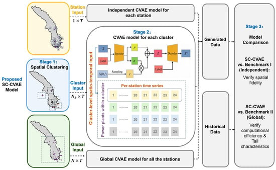
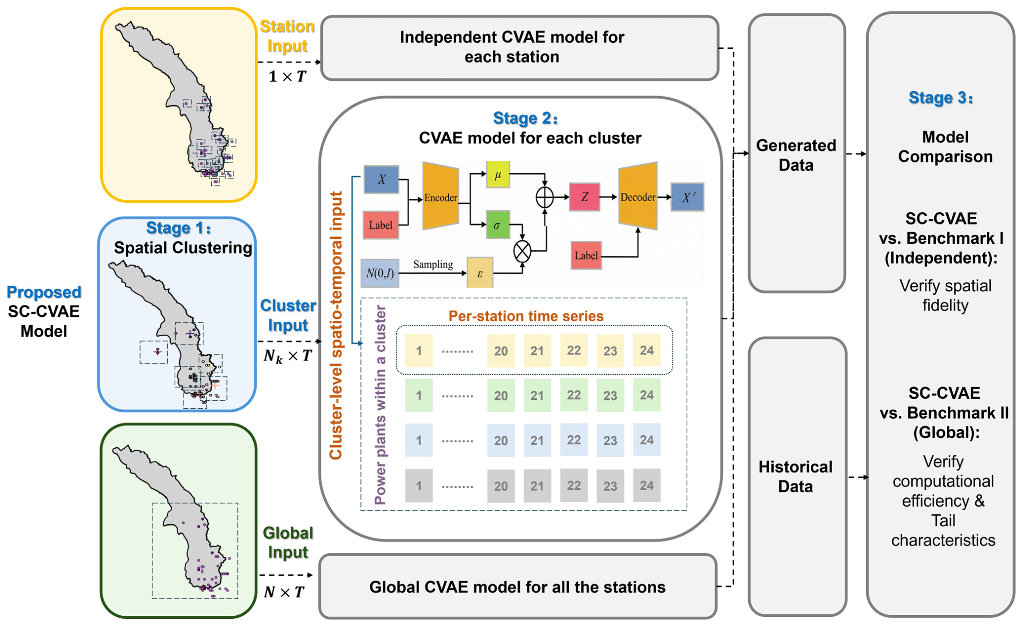
Direct joint modeling of extensive renewable energy stations poses a fundamental challenge in fitting high-dimensional joint probability distributions. To address this, this paper proposes a Spatial-Clustering Conditional Variational Auto-Encoder (SC-CVAE) framework. The core idea is a “divide-and-conquer” strategy that integrates physical spatial constraints with deep learning generative modeling, effectively re-balance the gradient signals between reconstruction and regularization. The framework operates in three stages, as shown in Figure 2:
Figure 2.
Overall architecture of the proposed SC-CVAE framework for high-dimensional joint distribution modeling. In the spatial maps, the dots represent individual power stations, the plus signs (+) indicate cluster centers, and the dashed boxes delineate the spatial boundaries for the cluster-level CVAE models. denotes the total number of candidate stations in the basin; T represents the temporal dimension of a single sample (e.g., 24 h); denotes the number of stations dynamically assigned to the specific cluster.
We first use the Fuzzy C-Means algorithm to spatially cluster all candidate stations into sub-clusters based on geospatial coordinates, decomposing the high-dimensional joint distribution into manageable local problems (Section 3.2). For each cluster, independent CVAE models are built to learn and reproduce the implicit joint probability distribution of all stations within that cluster, encompassing the adaptive architectural design and variational objectives (Section 3.3), as well as the data structuring, training, and scenario synthesis procedures (Section 3.4). To comprehensively validate the proposed SC-CVAE framework, we establish two distinct benchmark models. Benchmark I (Independent Baseline) is designed to quantify the loss of spatial fidelity when inter-station correlations are ignored. Benchmark II (Global Baseline) is constructed to demonstrate the superiority of the proposed clustering strategy in overcoming the curse of dimensionality and oversmoothing inherent in high-dimensional modeling. (Section 3.5). Finally, the quantitative evaluation indicators, specifically the Energy Score (ES) and Frobenius Norm Error, are introduced to rigorously assess the probabilistic fidelity and spatial coherence of the generated multi-energy scenarios (Section 3.6).
3.2. Spatial Clustering with Fuzzy C-Means (FCM)
We implement FCM clustering as a dynamic dimensionality reduction strategy. This approach preserves localized meteorological variability while ensuring computational tractability.
The FCM clustering algorithm [35], which dynamically groups individual stations into virtual cluster centers based on geospatial coordinates (latitude/longitude). While micro-topographical features such as elevation and surface roughness significantly impact local renewable outputs, they were deliberately excluded from this spatial decomposition phase. Including such features would generate highly fragmented partitions (e.g., artificially grouping geographically distant mountain peaks), thereby destroying the continuous macro-meteorological spatial boundaries necessary for basin-wide modeling. Instead, the localized impacts of these micro-topographical features are inherently captured and implicitly reconstructed by the subsequent CVAE model within each contiguous geographic cluster. Unlike hard clustering methods (e.g., K-means), FCM assigns probabilistic membership degrees, which better capture overlapping meteorological regimes across adjacent clusters.
The membership degree , representing the probability of the -th station belonging to the -th cluster, is iteratively updated as:
where denotes the feature vector of station , comprising its latitude/longitude. is the centroid of the -th cluster. is the number of clusters, is the number of total stations, and is the fuzziness index (set to 2 in this study). The index is used to denote alternative clusters when comparing distances.
The centroid for the -th cluster is updated using the following formula:
Here, denotes the membership degree raised to the power of the fuzziness index , which determines the weight of each station in computing the cluster center. This calculation adjusts the cluster center based on the weighted (by degree of membership) average of the data points.
The algorithm minimizes the objective function for the -th iteration, quantifying the weighted sum of squared distances between stations and cluster centroids:
This iterative process continues until the objective function converges. The stopping criterion is met when the change in between two consecutive iterations falls below a predefined threshold (set to 0.00001 in this study to guarantee numerical stability without excessive computational overhead):
To determine the optimal number of clusters, the Xie–Beni index [36,37] is employed, which explicitly penalizes small inter-cluster distances:
When computing the minimum distance, and refer to the centroids of two different clusters. The index assesses the clustering quality by balancing the compactness within clusters and the separation between clusters. A lower index value signifies more distinct clustering.
3.3. The SC-CVAE Architecture
Following the spatial decomposition, the second stage involves constructing deep generative models for each station cluster to learn their local joint probability distributions. This study adopts the Conditional Variational Auto-Encoder (CVAE) as the foundational architecture [38,39,40]. Compared to Generative Adversarial Networks (GANs), the CVAE offers explicit probabilistic modeling and superior training stability. Crucially, it extends the traditional Variational Auto-Encoder (VAE) [41] by integrating conditional variables—such as month labels—to guide the generation process, making it highly effective for capturing the seasonal characteristics inherent in renewable energy data. To ensure that the generative performance remains consistent across clusters of different scales, the model employs a structural design that adapts to the specific dimensionality of the input data.
3.3.1. Adaptive Network Architecture
Since the number of stations in each cluster varies significantly after clustering, using a fixed network structure would lead to a dilemma: underfitting for large clusters (insufficient capacity to capture complex correlations) and overfitting for small clusters. To address this, we designed a bounded adaptive architecture where the dimensions of hidden layers and the latent space are functions of . The original input dimension is defined as , which represents the total length of the flattened 1D feature vector derived from reshaping the 2D daily spatiotemporal matrix (detailed implementation is provided in Section 2.2). The specific task of this architecture is to use a 12-dimensional one-hot encoding vector (representing a specific month) as a condition to generate various stochastic daily generation patterns, rather than a single representative pattern.
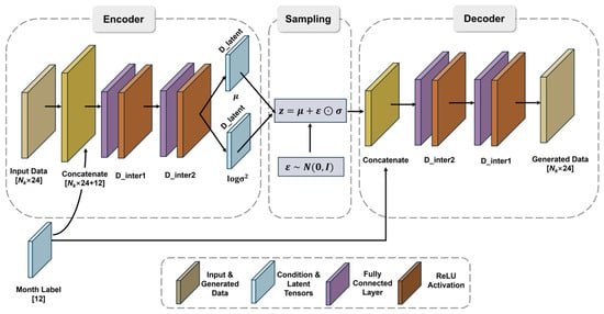
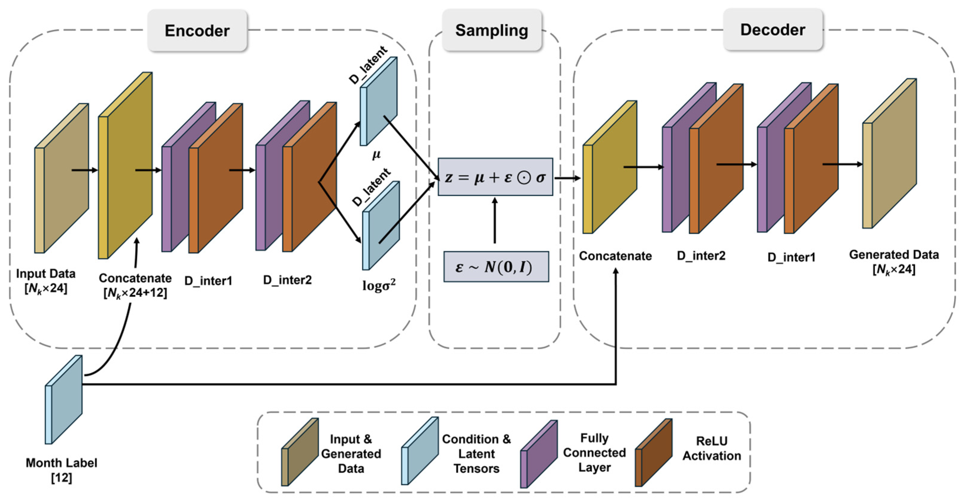
The adaptive network architecture is shown in Figure 3.
Figure 3.
Schematic diagram of the adaptive Spatial-Clustering Conditional Variational Auto-Encoder (SC-CVAE) network architecture. In the dimension notations, 24 represents the hourly time steps in a single daily temporal grid, and 12 corresponds to the 12-dimensional one-hot encoding vector used as the specific month condition. Note that [12] and [] indicate the dimensions of the tensors.
Wind power exhibits complex and dynamic spatial correlations driven by stochastic meteorological fluctuations. Therefore, a deeper and wider network configuration is adopted:
Solar power is primarily dominated by the deterministic diurnal cycle, resulting in relatively regular spatial patterns. Thus, the model configuration is adjusted to be more compact:
It should be noted that this bounded adaptive dimensioning strategy, along with the specific scaling constants and boundary limits in Equations (6)–(10), is not a universal theoretical approach, but rather a domain-specific engineering heuristic. These fixed bounds (e.g., 768, 1024, 1536, 2048) were determined through systematic hyperparameter observation and are intentionally set as multiples of 128 or 256 to optimize GPU memory alignment and computational efficiency. The model’s statistical fidelity exhibits low sensitivity to minor deviations from these exact integers (e.g., substituting 1024 with 1000 yields statistically negligible performance differences). However, the framework is highly sensitive to the absence of the bounds themselves. Removing the upper bounds inevitably triggers GPU Out-of-Memory (OOM) errors for large clusters, while removing the lower bounds causes severe overfitting for small clusters. Consequently, the adaptivity of the network dimensions is conditional—remaining dynamically scaled according to within an optimal operating range, but capped by these empirical bounds to guarantee training stability and generalizability.
3.3.2. Variational Objective and Composite Loss
To define the training objective for this complex multi-site model, a multi-objective composite loss function is constructed, incorporating reconstruction accuracy, latent space regularity, and temporal smoothness:
where is the reconstruction loss term, while and serve as hyperparameters that weigh the importance of the KL divergence regularization and the temporal smoothness constraint, respectively.
The model utilizes an Encoder–Decoder architecture. The encoder maps the input power data (the flattened spatiotemporal vector of dimension , and the condition vector (representing the 12-dimensional month labels) into a latent variable residing within a Gaussian latent space. To ensure the latent space is continuous and complete, the term is employed to force the approximate posterior to approximate a standard Gaussian prior :
where is the dimension of the latent space, while and denote the mean and variance of the latent dimension produced by the encoder, respectively.
To make the sampling process differentiable for backpropagation, the reparameterization trick is applied. Instead of sampling directly, we sample a noise variable from a standard Gaussian distribution and transform it:
This allows the gradients to flow through the deterministic parameters and , enabling end-to-end optimization of the network.
As for reconstruction Loss , we select different loss functions based on their distinct distributional characteristics and numerical stability requirements in deep learning. Wind power typically exhibits strong stochasticity and high volatility. When expressed as a capacity factor, the data points are distributed relatively continuously across the [0, 1] interval. MSE is based on the assumption of Gaussian noise and is sensitive to the magnitude of errors. It effectively penalizes large deviations, making it suitable for capturing the erratic and volatile fluctuations of wind profiles.
where denotes the total number of historical samples, is the sample index, represents the historical value, and is the model’s generated value. Note that represents the flattened spatiotemporal vector (dimension ), so the squared Euclidean norm implicitly sums the error over all time steps and stations.
Solar power, similarly expressed as the capacity factor, is characterized by a distinct bimodal distribution: a large number of zeros (nighttime) and a bell-shaped curve (daytime). In neural networks using Sigmoid activations to output [0, 1], MSE often suffers from vanishing gradients when values are close to the boundaries (0 or 1). BCE, derived from the Bernoulli likelihood, provides stronger gradients in these boundary regions [42]. This helps the model to sharply define the “sunrise” and “sunset” transitions and accurately reconstruct the specific shape of the solar curve, which is more deterministic than wind.
where is the total dimension of the flattened input features. Specifically, and denote the lth element of the flattened historical vector and the generated vector , respectively. The summation over ensures that the binary cross-entropy is calculated for every time step and every station.
For the final part, temporal smoothness constraint (). This optional term acts as a smoothness regularizer for wind power [43], penalizing unrealistic step-like changes between adjacent hours ( and ).
where represents the total number of time steps in the input sequence, and denotes the reconstructed power vector across all stations at time step .
3.4. Training and Generation
While Section 3.3 defines the theoretical architecture of the SC-CVAE, this section provides the concrete details regarding training parameters, and the final generation pipeline.
3.4.1. Model Training and Parameter Optimization
The SC-CVAE is trained by optimizing the encoder and decoder networks to minimize the composite loss function defined in Section 3.3.2. During this phase, the reparameterization trick is applied within the latent layer to maintain differentiability: the model samples noise from a standard Gaussian distribution and computes the latent variable.
We employ an Adam optimizer with a learning rate specifically tuned for different energy types (e.g., 10−4 for wind and 5 × 10⁻⁵ for solar). To prevent overfitting and ensure convergence, the training process incorporates an early stopping mechanism and a learning rate reduction strategy based on validation loss performance.
3.4.2. Scenario Sampling and Spatial Reconstruction
Following the completion of the training phase, the encoder is discarded, and the scenario generation task is handled entirely by the decoder model. The process begins with the sampling of a latent vector from a standard Gaussian distribution , which serves as a probabilistic representation of the stochastic fluctuations inherent in wind and solar resources. This noise vector is then combined with a specific 12-dimensional one-hot month label, which acts as a conditioning signal to guide the decoder toward the corresponding seasonal distribution. To finalize the output, the reconstructed vector is reshaped into its original temporal–spatial format. By repeating this sampling procedure for each independent cluster, the scenarios for each station of the entire energy base are obtained.
3.5. Benchmark Models Construction
To rigorously evaluate the performance of the proposed SC-CVAE framework, two benchmark models are established, each serving a specific purpose, as summarized in Table 1.
Table 1.
Summary of the proposed SC-CVAE and benchmark models for performance evaluation.
3.5.1. Benchmark I: Independent Baseline Model
The Independent Baseline Model is established to quantify the necessity of modeling spatial correlations by inherently ignoring inter-station dependencies. By treating each station as an independent entity, this benchmark focuses solely on capturing the unique temporal dynamics and stochastic volatility of individual sites, deliberately severing the spatial links that exist in the real-world physical system.
The modeling process is conducted on a station-by-station basis. For any given station, the basic processing unit is its historical power generation sequence. Similar to the proposed SC-CVAE, we incorporate a conditional vector (12-dimensional one-hot encoding of the month) to enable the model to perceive seasonal variations.
In terms of network architecture, we employ a standard CVAE framework tailored for univariate time-series generation. Since the input dimension for a single station is significantly lower than that of the joint model, we utilize a lightweight fully connected network. The Encoder consists of a three-layer fully connected network. It concatenates the flattened power vector and the condition vector as input, extracting temporal features through hierarchical dense layers with ReLU activations, finally mapping them to the Gaussian parameters of the latent space. The Decoder mirrors the encoder’s topology. It takes the sampled latent variable combined with the condition , and up-samples it back to the original data dimension through symmetrical dense layers. To prevent overfitting on single-station datasets, Dropout is applied between hidden layers. To ensure a fair comparison with the proposed method, the final output layer uses the Sigmoid activation function to constrain values within [0, 1], and the model is trained using the same composite loss function structure (Reconstruction Loss + KL Divergence).
This benchmark represents the limit of model performance when spatial information is completely absent. Comparing the SC-CVAE with this baseline allows us to explicitly isolate and quantify the gain in generative fidelity attributed to the spatial clustering and joint modeling strategy.
3.5.2. Benchmark II: Global Baseline Model
To assess the scalability and generative stability of the proposed method, we define a Global Baseline Model representing the traditional monolithic deep generative approach.
Unlike the divide-and-conquer strategy of SC-CVAE, this model treats the entire multi-energy system as a single high-dimensional entity. It directly inputs the joint time-series data of all stations into one unified CVAE network.
This model adopts the SC-CVAE framework (as detailed in Section 3.3), which the network depth and width are dynamically scaled according to the global input dimension. This baseline is specifically used to highlight computational bottlenecks and the “posterior collapse” phenomenon—a failure mode where the model ignores the stochastic latent variables and instead outputs overly smooth, average-level scenarios to minimize total reconstruction error. This phenomenon occurs when existing deep generative models attempt to process massive-scale renewable energy systems without structural decomposition.
3.6. Scenario Evaluation Indicators
To quantitatively evaluate the quality of the generated multi-energy scenarios, ensuring they possess both high probabilistic fidelity and accurate spatial coherence, this study employs two complementary metrics: the Energy Score (ES), and the Frobenius Norm Error ().
- (1)
- Energy Score (ES)
The Energy Score is a proper scoring rule for multivariate distributions and is widely regarded as a standard metric for evaluating probabilistic forecasts [44]. It assesses both the accuracy (distance to data) and the diversity (variability) of the scenarios generated. For a historical data vector and a set of generated scenario samples , the analytical estimator of ES is defined as:
where denotes the total number of generated scenarios, and are independent generated scenario samples drawn from the generative model; represents the ground-truth historical data; and denotes the Euclidean norm.
The first term measures the distance between the generated scenarios and reality, capturing accuracy, while the second term measures the expected pairwise distance among the generated scenarios and , reflecting diversity. A lower ES indicates a better distributional fit.
- (2)
- Frobenius Norm Error (EF)
To directly quantify the global deviation of the generated spatial correlation matrix from the historical one, we use the Frobenius Norm, a fundamental component in matrix distance measures [45]. This metric serves as a numerical validation for the correlation heatmaps:
where and denote the spatial correlation matrices derived from the generated scenarios and the historical scenarios, respectively. The terms and represent the specific Pearson correlation coefficient between station and station within the generated and historical datasets. A lower indicates a more precise reproduction of the global spatial correlation matrix.
4. Results and Discussion
4.1. Spatial Clustering Results
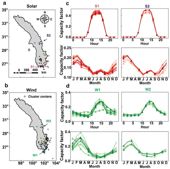
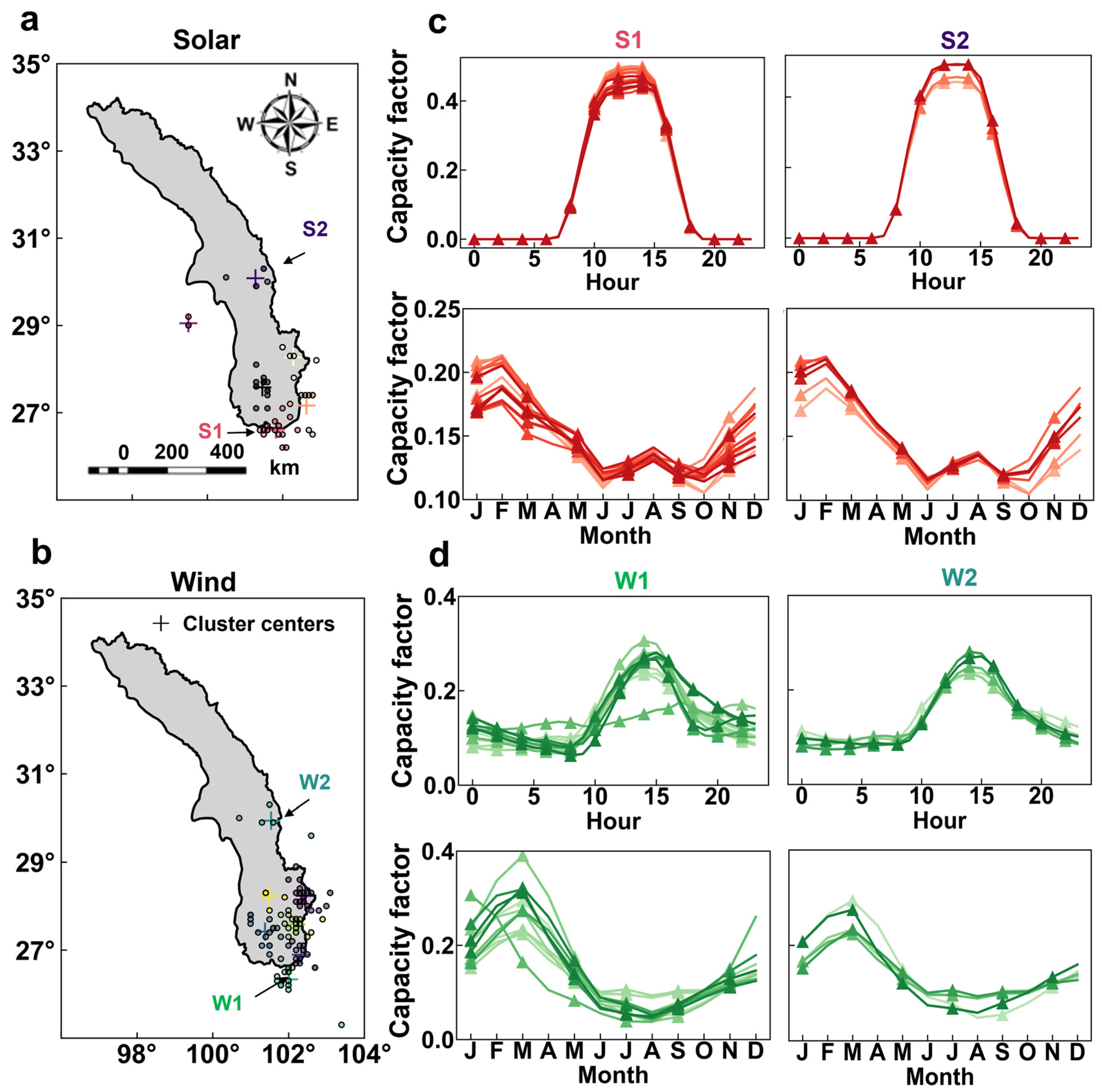
The proposed spatial clustering strategy proved effective in decomposing the high-dimensional multi-energy system into physically distinct and computationally manageable sub-regions, thereby establishing a robust foundation for the SC-CVAE framework. Guided by the Xie–Beni validity index, which balances intra-cluster compactness and inter-cluster separation, we identified the optimal partition for the Yalong River basin. As shown in Figure 4a,b, the XB index reached its minimum at 7 clusters for wind power and 6 for solar power, respectively (an ablation analysis validating this optimal configuration is detailed in Appendix D). The detailed list of stations assigned to each cluster and their geographical coordinates are provided in Appendix A.
Figure 4.
Spatial clustering results for wind (W) and solar (S) stations. (a,b) Optimal configurations with 7 wind and 6 solar clusters (dots: stations; plus signs: cluster centers). (c,d) Diurnal and seasonal profiles of representative clusters. Two typical clusters for each energy type (S1, S2 and W1, W2) are selected for visualization to illustrate intra-cluster patterns while avoiding severe visual clutter. Each line in (c) and (d) represents the exact capacity factor profile of all individual station within the respective cluster.
The resulting clusters exhibit strong geographic coherence and meaningful meteorological interpretability. As illustrated in the diurnal and seasonal profiles (Figure 4c,d), the algorithm successfully groups stations with synchronized temporal patterns and similar output characteristics while maintaining distinct aggregate profiles between different clusters. Crucially, by decomposing the system based on these underlying meteorological regimes, the modeling dimensionality is significantly reduced from hundreds of stations to parallel, low-dimensional sub-problems. This effectively mitigates the curse of dimensionality, ensuring the stability and convergence of the subsequent CVAE training.
It is crucial to emphasize that the success of this divide-and-conquer strategy stems specifically from its geospatial conditioning, rather than mere mathematical dimensionality reduction. In pure machine learning, arbitrary or random grouping could technically reduce the input dimension. However, renewable energy generation is governed by continuous meteorological systems. Arbitrary grouping would force the CVAE to learn spurious, non-physical correlations across distant stations, essentially fitting statistical noise. By employing FCM-based geospatial clustering, the deep learning architecture is explicitly aligned with the underlying physical boundaries of macro-meteorological regimes. This physically informed decomposition guarantees that each sub-CVAE models genuine weather synergies, which is the foundational prerequisite for accurately reconstructing the global spatial correlation matrix.
4.2. Evaluation of Statistical Consistency for Generated Time Series
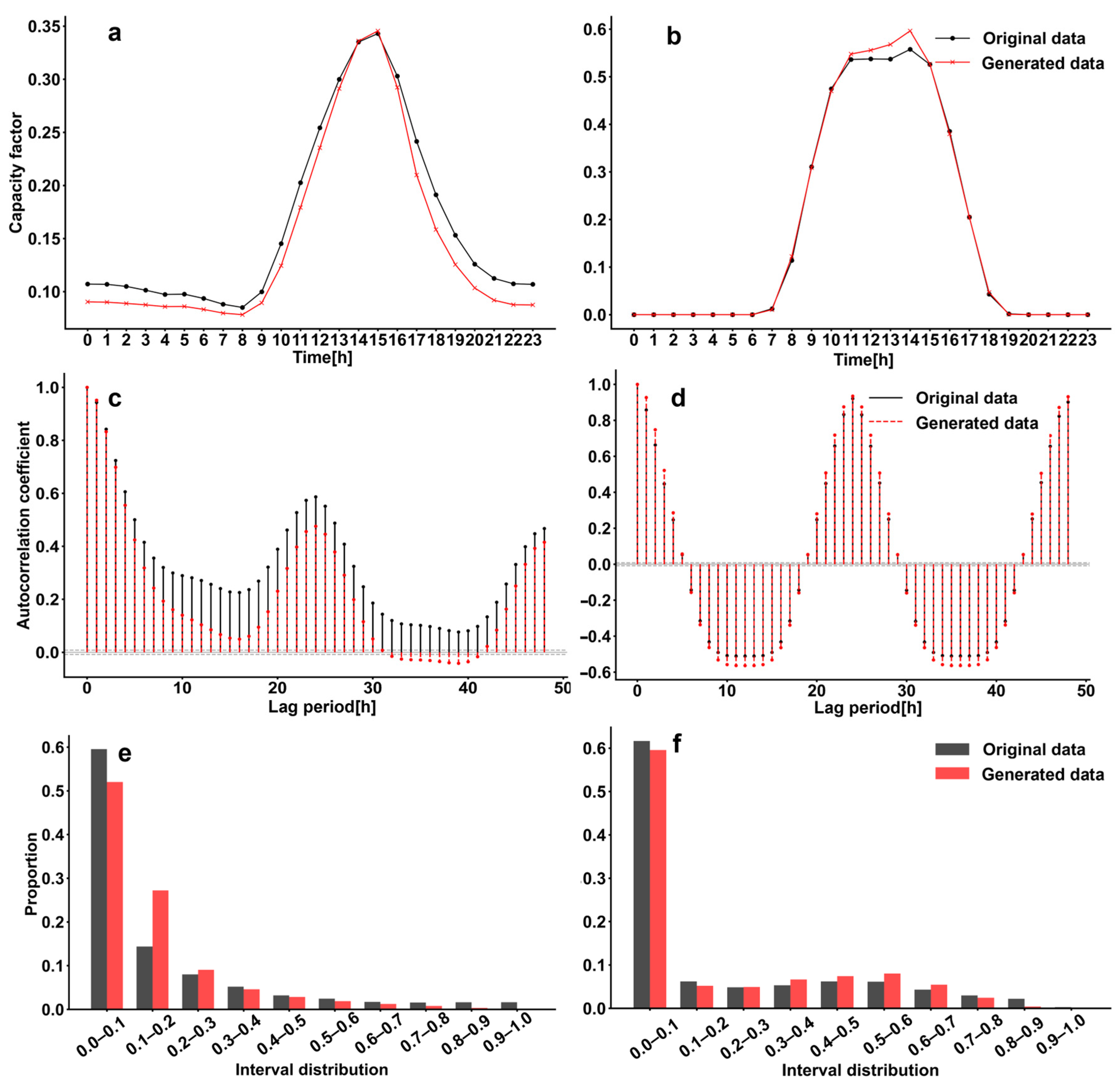
The comparative analysis against historical data confirms that the proposed SC-CVAE model reproduces the fundamental statistical characteristics and temporal dynamics of the wind and solar resources. To quantitatively assess the authenticity of the generated data, this study conducts a comparative analysis between the generated scenarios and the original data. Specifically, a representative wind station and a solar station are selected from the study cluster to demonstrate individual site-level fidelity across three dimensions: capacity factor amplitude statistics (mean and distribution) and temporal correlation (Figure 5). While the model exhibits strong alignment in most metrics, minor deviations are observed in the short-term persistence of wind power and extreme high-output events, reflecting the inherent difficulty in modeling highly stochastic energy sources.
Figure 5.
Validation of multi-dimensional statistical consistency for generated wind and solar power capacity factor scenarios at the individual site level. The comparisons illustrate the performance in annual average diurnal trends (a,b), temporal autocorrelation functions (ACF) derived from continuous time-series segments (c,d), and annual probability density distributions. (e,f) Subplots (a,c,e) correspond to a representative wind station, while (b,d,f) correspond to a representative solar station.
First, regarding diurnal patterns, Figure 5a,b illustrate the annual average hourly capacity factor. The generated data (red lines) achieve a high degree of alignment with the original data (black lines). These results demonstrate that the model has effectively learned the distinct average daily variation laws of different energy sources.
Second, regarding internal time dependencies, the Autocorrelation Function (ACF) is calculated based on a continuous chronological sequence (48 h). As shown in Figure 5d, the model exhibits high precision for solar power due to the strong physical determinism of solar irradiance. In contrast, the performance for wind power (Figure 5c), which possesses stronger stochasticity, shows a slight deviation where generated ACF values are systematically lower than the original. This suggests that while the general 24 h periodicity is retained, the short-term persistence in generated wind scenarios is marginally weaker than in real data due to its rapid fluctuations and intermittency.
Finally, the probability density distributions (Figure 5e,f) provide critical insight into the model’s generative behavior at the individual site level. The model maintains excellent morphological consistency, with the Root Mean Square Error (RMSE) controlled at approximately 0.05 for wind and 0.02 for solar. Despite this high overall accuracy, distinct deviations are observed in specific intervals. For wind power, the generated data exhibits a slight overestimation in the low-output range (0.1–0.2), contrasting with a underestimation in the high-output range (0.8–1.0). Similarly, solar power shows a minor probability deficit in the high-output region.
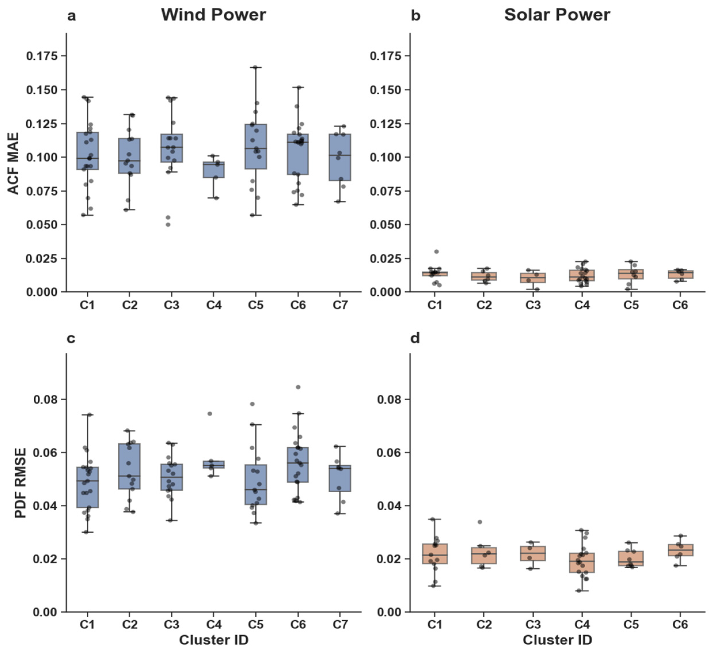
To further demonstrate the robustness of the SC-CVAE across all sites and avoid selective bias, we provide the aggregate statistical error distributions for all individual stations across all clusters in Appendix C. Specifically, we evaluate the model’s distributional accuracy via the Root Mean Square Error of the Probability Density Function (PDF RMSE), and its temporal consistency via the Mean Absolute Error of the Autocorrelation Function (ACF MAE). The consistent performance across the entire basin confirms the model’s capability in capturing high-dimensional statistical fidelity.
This systemic smoothing effect is primarily attributed to the inherent characteristics of the VAE objective function. In multi-station modeling, the reconstruction error (MSE/BCE) often significantly outweighs the KL divergence term, causing the reconstruction loss to dominate the optimization process. This imbalance frequently triggers “posterior collapse”, leading the model to output conservative, average-level scenarios to minimize the total error. Consequently, a small fraction of extreme events—whether low or high intervals—are smoothed out. While this mechanism ensures robustness, it results in a conservative evaluation of extremes, an effect that is particularly pronounced in wind power due to its higher volatility compared to solar.
4.3. Reconstruction of High-Dimensional Spatial Correlations
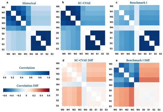
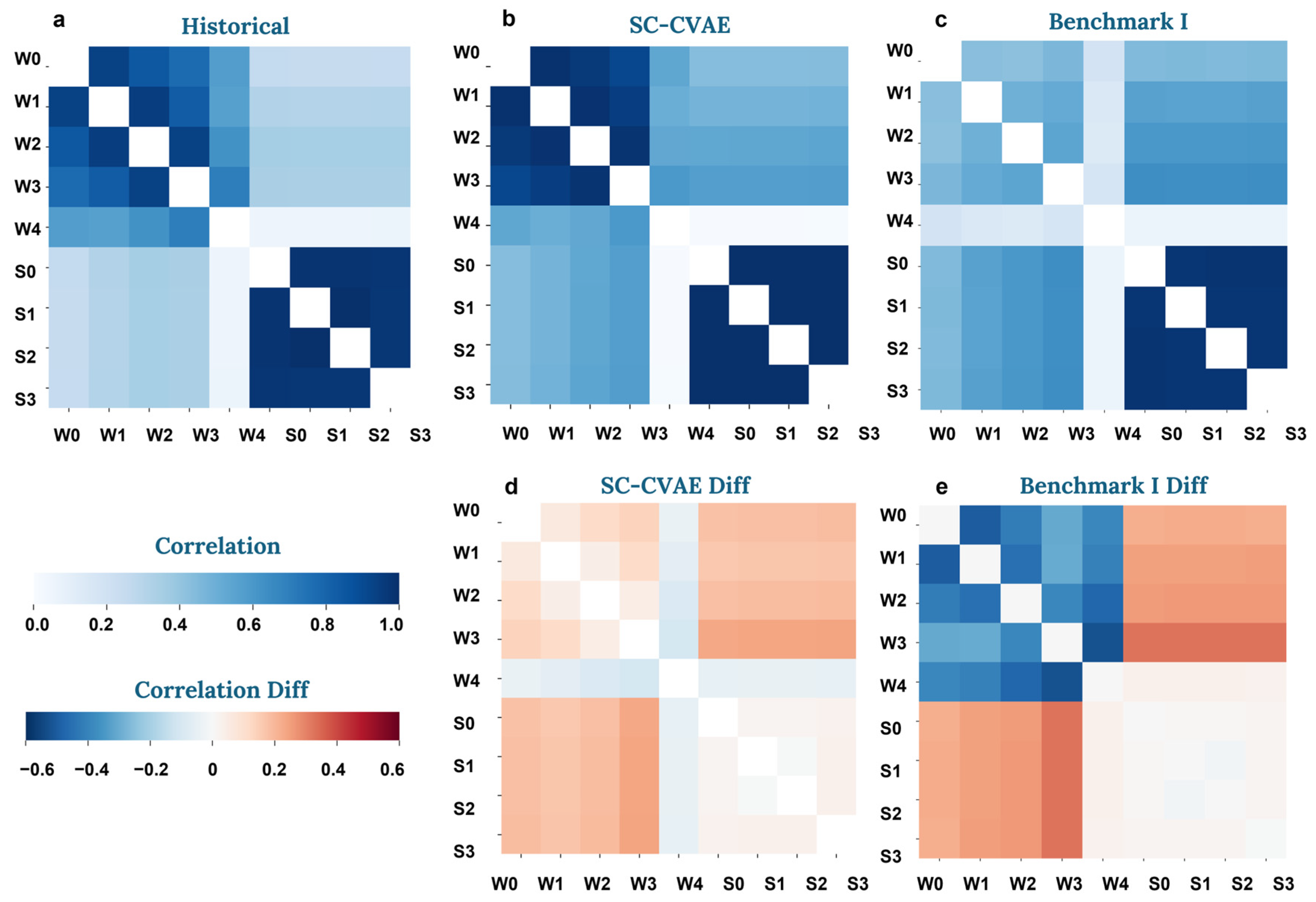
To quantitatively evaluate the reconstruction of high-dimensional spatial correlations, we select the power stations within Wind Cluster 4 and PV Cluster 3 as a representative case study. The evaluation utilizes the Pearson correlation coefficient matrix to measure the dependencies among these stations. The calculation begins by flattening the 3D scenario data—consisting of months, scenarios, and hourly time points—into a 2D matrix of shape containing stations and time. The Pearson coefficient between any two stations is then computed to form the spatial correlation matrices.
The proposed SC-CVAE framework demonstrates superior performance in reconstructing high-dimensional spatial correlations compared to Benchmark I (Independent Baseline). As illustrated in Figure 6, the heatmap generated by the SC-CVAE (Figure 6b) exhibits high fidelity to the historical data (Figure 6a), accurately maintaining the heterogeneous dependency patterns of the basin. This accuracy is further validated by the SC-CVAE Diff map (Figure 6d), which remains predominantly near-zero, confirming that the gap between the generated scenarios and historical scenarios are minimized across both wind and solar clusters. The minor intensifications in correlation observed in the SC-CVAE results are attributed to the model’s generative nature, which effectively captures dominant meteorological trends while filtering out the non-systematic local noise that typically dilutes correlations in raw data. In contrast, Benchmark model I (Independent Baseline, Figure 6c) illustrates a significant loss of cross-station correlations due to its independent modeling assumption. Since it ignores spatial synergies, the correlation structures are almost entirely absent. This is explicitly visualized in the Benchmark I Diff map (Figure 6e), which displays widespread and substantial deviations from the historical truth.
Figure 6.
Visualization of spatial correlation matrices (Pearson coefficient) for wind and solar power stations (a) Historical data, showing complex meteorological dependencies; (b) Scenarios generated by the proposed SC-CVAE, visually preserving the historical correlation structures; (c) Scenarios generated by Benchmark model I (Independent Baseline), illustrating the loss of cross-station correlations due to independent modeling assumptions; (d) SC-CVAE Diff, the difference between SC-CVAE and historical data; (e) Benchmark I Diff, the difference between Benchmark I and historical data.
As summarized in Table 2, the quantitative metrics of Frobenius Norm Error across different scopes evaluate the deviations between the generated and the historical correlation matrices and confirm the SC-CVAE’s dominant performance, as evidenced by the lowest Frobenius Norm Error across all scopes.
Table 2.
Quantitative comparison of spatial correlation metrics (Frobenius Norm Error).
The specific quantitative and physical improvements are analyzed as follows: For wind stations, the SC-CVAE drastically reduces the Frobenius Norm Error for wind power by 74% (from 1.518 to 0.394) compared to the Benchmark. High historical correlations in wind are driven by synchronized fluctuations from real-time weather systems. While the Benchmark model effectively filters out these shared systems by retaining only the seasonal baseline, the SC-CVAE’s joint modeling strategy preserves these critical inter-station dependencies.
For solar stations, the SC-CVAE achieves an extremely low error (0.075), comparable to the Benchmark (0.078). This is because solar power is primarily dominated by strong seasonal and astronomical drivers with high regional synchronicity, which renders the impact of stochastic weather fluctuations—the primary drivers in other energy sources—relatively secondary to these deterministic cycles. The SC-CVAE accurately captures these deterministic drivers, ensuring that the inherent high correlation of solar generation is preserved.
Although wind and solar clusters are modeled independently within the SC-CVAE framework, the results show a significant reduction in global correlation error by 56% (from 2.710 to 1.181) compared to the Benchmark. The superior performance in this metric is primarily attributed to the high-fidelity reconstruction of type-wise spatial structures. By accurately capturing the internal variance and regional synchronicity of each energy type, the SC-CVAE prevents the spurious enhancement of seasonal correlations observed in the Benchmark, thereby maintaining a more realistic global dependency structure.
4.4. Computational Efficiency and Preservation of Extreme Volatility
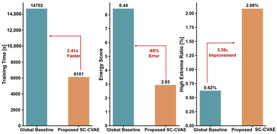
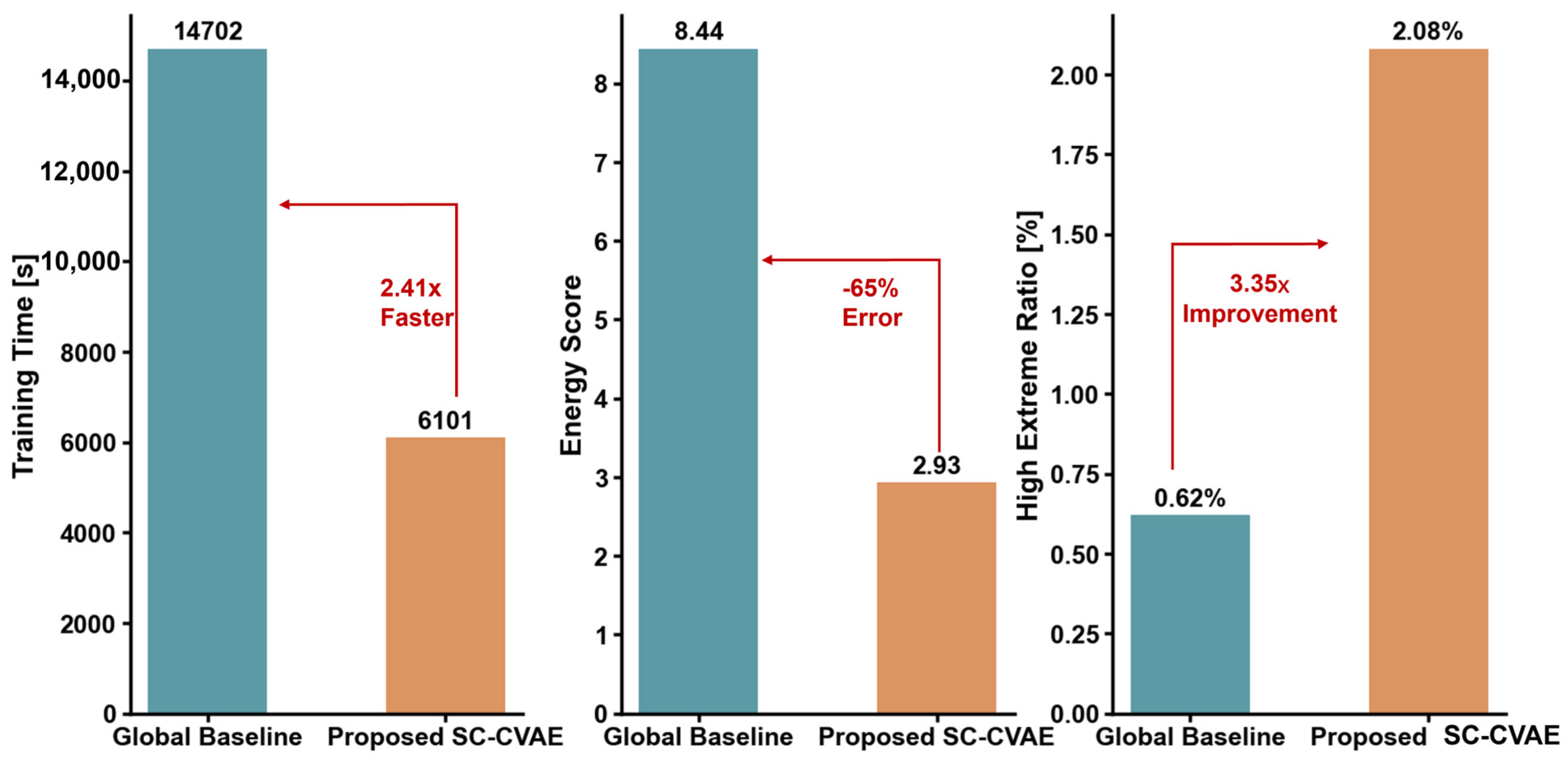
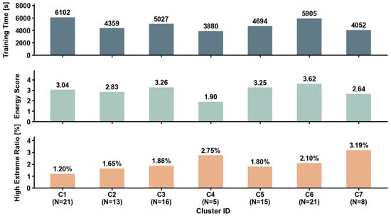
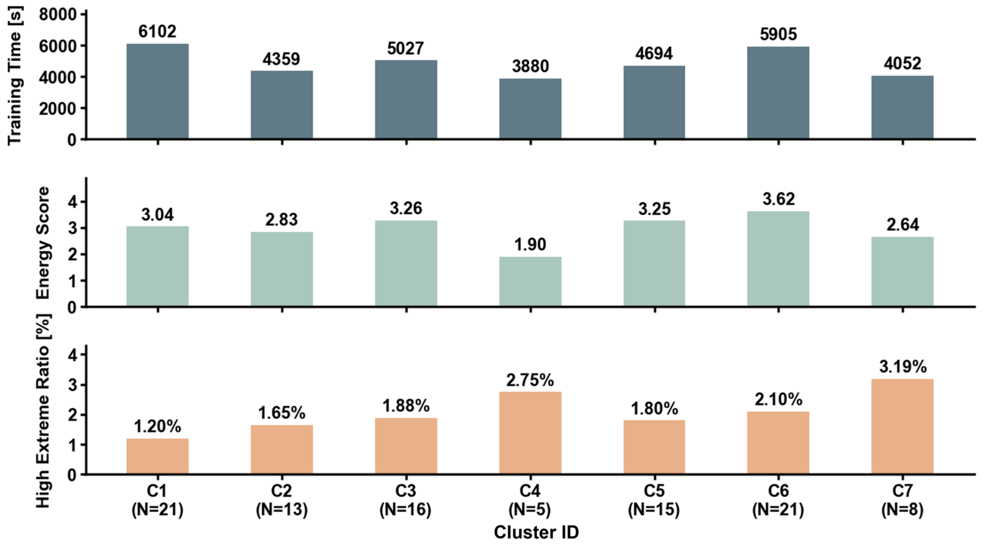
The proposed SC-CVAE framework achieves a superior balance between computational efficiency and generative fidelity, effectively overcoming the curse of dimensionality through its cluster-based decomposition strategy. To evaluate the model’s capability in capturing tail risks, we introduced a “High Extreme” indicator, defined as the ratio of generated samples surpassing the 95th percentile threshold of the historical data. For the SC-CVAE evaluation, the whole training time is defined as the maximum duration among parallel clusters—representing the parallel processing bottleneck (the comprehensive training protocol, including early stopping criteria and hardware configurations, is detailed in Appendix B). Meanwhile, the Energy Score (ES) and High Extreme indicators are calculated as the average values across all spatial clusters to represent system-wide performance. As summarized in Figure 7, the framework significantly outperforms the Global Baseline (modeling all stations jointly) across all key metrics, including training speed, energy score, and the capture of extreme events. The specific performance metrics for individual spatial clusters are detailed in Figure 8.
Figure 7.
Comprehensive Performance Comparison: Global Baseline vs. Proposed SC-CVAE.
Figure 8.
Comprehensive performance evaluation of individual spatial clusters across computational efficiency, probabilistic fidelity, and extreme capture capabilities.
The SC-CVAE achieves a 2.41-fold speedup in training efficiency by leveraging the parallel processing capability of independent spatial clusters. While the Global Baseline required 14,702 s (4.08 h) to converge due to high-dimensional complexity, the effective wall-clock training time for the SC-CVAE is determined only by the bottleneck cluster. According to Figure 8, Cluster 1 represented this bottleneck with a maximum duration of 6101 s (roughly 41% of the baseline cost), demonstrating superior scalability for large-scale energy systems. From an engineering perspective, the transition from hours to minutes is critical. Although capacity planning is a long-term task, robust design and sensitivity analysis often require thousands of iterative simulations across varying climate scenarios and configurations. This acceleration proves that the decomposition strategy effectively counters the curse of dimensionality, ensuring the numerical stability and high-frequency iteration capability necessary for large-scale energy systems.
Generative quality is significantly enhanced, with the SC-CVAE reducing the ES error by 65% compared to the monolithic model. The Global Baseline yielded a poor fit with an ES of 8.44, whereas the SC-CVAE achieved a remarkably lower cluster-averaged ES of 2.93. This improvement validates the re-balancing of gradient signals. For high-dimensional input, the reconstruction loss contains the error sum of thousands of elements, creating a numerical magnitude that dominates the loss function and suppresses the regularization effect of the KL divergence constraint on the latent space. Experimental data from Figure 8 confirm this: smaller clusters, such as Cluster 4 (5 stations), achieved the best fidelity with an ES as low as 1.90. Even Cluster 6, which involves complex terrain and a larger number of stations (21 stations, ES = 3.62), significantly outperformed the Global Baseline. This proves that reducing the dimension of individual sub-problems prevents the reconstruction loss from overwhelming the feature learning of latent variables, thereby significantly improving the fitting precision of the posterior distribution.
Crucially, we examine the model’s ability to reproduce extreme events and volatility. A common failure in generative modeling is Posterior Collapse, which should not be viewed merely as a technical instability, but as a fundamental threat to power system risk assessment and energy security. In this context, the oversmoothing caused by posterior collapse essentially forces the model to simulate a misleading average state. From an engineering perspective, these over-smoothed scenarios mask the synchronous risks inherent in river basins—such as widespread “wind droughts” or simultaneous solar drops—thereby creating a dangerous underestimation of potential power supply deficits.
This phenomenon is evident in the Global Baseline, where the standard deviation of the generated scenarios is severely underestimated (0.15 vs. Real 0.23), and only 0.62% of high-extreme events are captured. In contrast, the SC-CVAE successfully restores the statistical dynamics of the system. It improves the average high-extreme capture ratio to 2.08% (Figure 7, a 3.35-fold improvement). This overall enhancement is fundamentally driven by the localized modeling strategy, as evidenced by the performance of individual clusters in Figure 8. Specifically, smaller clusters such as Cluster 4 (5 stations) achieve the highest fidelity with an ES as low as 1.90. Even Cluster 6, despite its complex terrain and larger scale (21 stations, ES = 3.62), significantly outperforms the Global Baseline. From an analytical perspective, this superior fidelity stems from a more optimal balance between the reconstruction loss and the KL divergence regularization within lower-dimensional subspaces. While the high-dimensional Global Baseline falls into the oversmoothing trap because reconstruction error dominates the gradient, our method prevents this by matching model capacity to physical dimensionality. This is most evident in Cluster 7 (8 stations), where the model automatically configures a more compact network depth, achieving an extreme capture ratio of 3.19%—a level far exceeding the 0.62% of the Global Baseline. These findings indicate that high-fidelity restoration of tail risks is of paramount engineering significance for robust renewable energy planning.
5. Conclusions
Addressing the critical challenges of high-dimensional uncertainty and the curse of dimensionality in large-scale Multi-Energy Complementary Systems, this paper proposes a Spatial-Clustering Conditional Variational Auto-Encoder (SC-CVAE) Framework. By explicitly integrating physical spatial constraints into deep generative modeling, the proposed framework achieves a balance between computational tractability and statistical fidelity. The main conclusions are as follows:
- The proposed paradigm, integrating spatial clustering with deep generation, breaks the computational bottleneck inherent in high-dimensional joint modeling. Empirical evidence demonstrates that by decomposing the state space into manageable physical clusters, the SC-CVAE achieves a 2.41-fold speedup in training efficiency compared to the global baseline
- Unlike independent modeling approaches that sever inter-station dependencies, the SC-CVAE precisely reproduces the complex spatiotemporal synergistic effects. It reduces the global spatial correlation error (measured by the Frobenius Norm) by 56% compared to the independent benchmark, ensuring the generated scenarios reflect the synchronous risks of the basin.
- The framework effectively mitigates the posterior collapse and oversmoothing effects inherent in high-dimensional VAEs. By re-balancing gradient signals through structural decomposition, it reduces the Energy Score (ES) error by 65% and improves the capture ratio of high-impact extreme events by 3.35-fold compared to the global baseline.
The SC-CVAE framework exhibits superior scalability for large-scale energy bases. Since the training complexity of the framework is primarily determined by the “bottleneck cluster” (the largest individual sub-problem) rather than the total number of stations, it demonstrates significant potential for application in provincial or even larger power systems. The current SC-CVAE framework utilizes standard one-hot encoding to represent seasonal conditions (months). While the extensive historical dataset enables the network to implicitly capture seasonal continuity, one-hot encoding inherently treats time steps as equidistant, thereby neglecting the cyclical nature of meteorological seasons. Future research will replace this with trigonometric cyclical embeddings (Sine/Cosine encoding) to explicitly preserve the periodic distance between adjacent periods, further enhancing the temporal coherence of the generated scenarios. While wind and solar clusters are currently modeled as independent entities to ensure computational stability in high-dimensional spaces, this modular structure serves as a critical foundation for multi-energy modeling. Future work will focus on integrating cross-type coupling mechanisms into the SC-CVAE architecture. By establishing inter-energy dependency links between the already refined wind and solar modules, we aim to achieve a comprehensive joint generative paradigm that captures deep synergies across all energy types.
Author Contributions
J.H. conceived the research and performed the research. J.H. and Z.L. analyzed the results and drafted the manuscript. B.X. and H.Z. provided comments and revised the manuscript. All authors have read and agreed to the published version of the manuscript.
Funding
This work was supported by the National Natural Science Foundation of China (No. U2340210, No. 52441901 and No. 52309008).
Data Availability Statement
The original contributions presented in the study are included in the article; further inquiries can be directed to the corresponding author.
Conflicts of Interest
The authors declare no conflicts of interest.
Abbreviations
The following abbreviations are used in this manuscript:
| HESs | Hybrid Energy Systems |
| SC-CVAE | Spatial-Clustering Conditional Variational Auto-Encoder |
| FCM | Fuzzy C-Means |
| XB | Xie–Beni index |
| VRE | Variable Renewable Energy |
Appendix A
Table A1.
Summary of Wind Power Clustering Characteristics.
Table A2.
Summary of Solar Power Clustering Characteristics.
Appendix B
Table A3.
Detailed hyperparameter settings and hardware configurations for model training.
Appendix C
To evaluate the generalizability of the SC-CVAE framework across the entire stations, we calculated the reconstruction errors for all stations within the identified clusters.
Figure A1.
Aggregate statistical error distributions for all wind (7 clusters) and solar (6 clusters) stations. (a) ACF MAE for Wind clusters; (b) ACF MAE for Solar clusters; (c) PDF RMSE for Wind clusters; (d) PDF RMSE for Solar clusters. Each gray dot represents an individual station, while the boxplots illustrate the median, quartiles, and range of errors within each physical cluster.
Appendix D
It is crucial to emphasize that the generative outcomes of the SC-CVAE framework remain robust to minor deviations in the choice of cluster number in the XB index. To explicitly illustrate this robustness, we evaluated a suboptimal configuration for the solar stations by artificially reducing the cluster number to .
As detailed in Table A4, under the optimal K = 6 configuration, the solar framework achieved an average Energy Score (ES) of 2.45 and an extreme event capture ratio of 2.65%. When forced into the suboptimal K = 5 configuration, the average ES experienced only a minor degradation to 2.58, and the extreme event capture ratio decreased slightly to 2.41%. This graceful degradation—rather than a catastrophic performance collapse—confirms that the deep generative architecture is robust. Even with slight deviations in spatial partitioning, the SC-CVAE framework consistently maintains generative fidelity, thereby guaranteeing the stability and generalizability of the overall conclusions.
Table A4.
Robustness of generative performance to the choice of cluster number (Solar power).
References
- Hu, J.; Li, Y.; Wörman, A.; Zhang, B.; Ding, W.; Zhou, H. Reducing Energy Storage Demand by Spatial-Temporal Coordination of Multienergy Systems. Appl. Energy 2023, 329, 120277. [Google Scholar] [CrossRef] [Scilit]
- Ming, B.; Liu, P.; Cheng, L. An Integrated Framework for Optimizing Large Hydro–Photovoltaic Hybrid Energy Systems: Capacity Planning and Operations Management. J. Clean. Prod. 2021, 306, 127253. [Google Scholar] [CrossRef] [Scilit]
- Xu, B.; Liu, Z.; Yan, S.; Schmitt, R.J.P.; He, X. Strategizing Renewable Energy Transitions to Preserve Sediment Transport Integrity. Nat. Sustain. 2025, 8, 1314–1327. [Google Scholar] [CrossRef] [Scilit]
- Powell, W.B.; Meisel, S. Tutorial on Stochastic Optimization in Energy—Part I: Modeling and Policies. IEEE Trans. Power Syst. 2016, 31, 1459–1467. [Google Scholar] [CrossRef] [Scilit]
- Liu, Z.; Mo, L.; Zhang, M.; Kang, J.; Liu, W.; Sun, X.; Xiao, W. High-Dimensional Scenario Generation Method Joint-Driven by Multiple Correlations for Hydro-Wind-Photovoltaic. Appl. Energy 2025, 400, 126551. [Google Scholar] [CrossRef] [Scilit]
- Chen, Y.; Wang, Y.; Kirschen, D.; Zhang, B. Model-Free Renewable Scenario Generation Using Generative Adversarial Networks. IEEE Trans. Power Syst. 2018, 33, 3265–3275. [Google Scholar] [CrossRef] [Scilit]
- Collins, S.; Deane, P.; Ó Gallachóir, B.; Pfenninger, S.; Staffell, I. Impacts of Inter-Annual Wind and Solar Variations on the European Power System. Joule 2018, 2, 2076–2090. [Google Scholar] [CrossRef] [Scilit]
- Lee, J.; Dessler, A.E. The Impact of Neglecting Climate Change and Variability on ERCOT’s Forecasts of Electricity Demand in Texas. Weather Clim. Soc. 2022, 14, 499–505. [Google Scholar] [CrossRef] [Scilit]
- Zheng, K.; Sun, Z.; Song, Y.; Zhang, C.; Zhang, C.; Chang, F.; Yang, D.; Fu, X. Stochastic Scenario Generation Methods for Uncertainty in Wind and Photovoltaic Power Outputs: A Comprehensive Review. Energies 2025, 18, 503. [Google Scholar] [CrossRef] [Scilit]
- Usaola, J. Synthesis of Hourly Wind Power Series Using the Moving Block Bootstrap Method. In Proceedings of the2014 International Conference on Probabilistic Methods Applied to Power Systems, PMAPS 2014—Conference Proceedings; IEEE: New York, NY, USA, 2014. [Google Scholar] [CrossRef] [Scilit]
- Teichgraeber, H.; Brandt, A.R. Clustering Methods to Find Representative Periods for the Optimization of Energy Systems: An Initial Framework and Comparison. Appl. Energy 2019, 239, 1283–1293. [Google Scholar] [CrossRef] [Scilit]
- Hoffmann, M.; Kotzur, L.; Stolten, D.; Robinius, M. A Review on Time Series Aggregation Methods for Energy System Models. Energies 2020, 13, 641. [Google Scholar] [CrossRef] [Scilit]
- Xie, J.; Liu, Z.; Yan, S.; Ziegler, A.D.; Shi, X.; Xu, B.; Srinuansom, K.; Peng, X.; Yoshimura, K.; He, X. Variable Renewable Energy Pathways in the Lower Mekong Basin under Projected River Flow Extremes. Commun. Earth Environ. 2025, 6, 928. [Google Scholar] [CrossRef] [Scilit]
- Huang, Y.; Zhang, Z.; Li, X.; Xie, J.; Lee, K.Y. Layered-Vine Copula-Based Wind Speed Prediction Using Spatial Correlation and Meteorological Influence. IEEE Trans. Instrum. Meas. 2023, 72, 1010312. [Google Scholar] [CrossRef] [Scilit]
- Wang, Y.; Ma, H.; Wang, D.; Wang, G.; Wu, J.; Bian, J.; Liu, J. A New Method for Wind Speed Forecasting Based on Copula Theory. Environ. Res. 2018, 160, 365–371. [Google Scholar] [CrossRef] [Scilit]
- Goh, H.H.; Peng, G.; Zhang, D.; Dai, W.; Kurniawan, T.A.; Goh, K.C.; Cham, C.L. A New Wind Speed Scenario Generation Method Based on Principal Component and R-Vine Copula Theories. Energies 2022, 15, 2698. [Google Scholar] [CrossRef] [Scilit]
- Morales, J.M.; Mínguez, R.; Conejo, A.J. A Methodology to Generate Statistically Dependent Wind Speed Scenarios. Appl. Energy 2010, 87, 843–855. [Google Scholar] [CrossRef] [Scilit]
- Zhang, H.; Lu, Z.; Hu, W.; Wang, Y.; Dong, L.; Zhang, J. Coordinated Optimal Operation of Hydro–Wind–Solar Integrated Systems. Appl. Energy 2019, 242, 883–896. [Google Scholar] [CrossRef] [Scilit]
- Pinson, P.; Madsen, H.; Nielsen, H.A.; Papaefthymiou, G.; Klöckl, B. From Probabilistic Forecasts to Statistical Scenarios of Short-Term Wind Power Production. Wind Energy 2009, 12, 51–62. [Google Scholar] [CrossRef] [Scilit]
- Papaefthymiou, G.; Klöckl, B. MCMC for Wind Power Simulation. IEEE Trans. Energy Convers. 2008, 23, 234–240. [Google Scholar] [CrossRef] [Scilit]
- Tang, C.; Wang, Y.; Xu, J.; Sun, Y.; Zhang, B. Efficient Scenario Generation of Multiple Renewable Power Plants Considering Spatial and Temporal Correlations. Appl. Energy 2018, 221, 348–357. [Google Scholar] [CrossRef] [Scilit]
- Schreiber, J.; Jessulat, M.; Sick, B. Generative Adversarial Networks for Operational Scenario Planning of Renewable Energy Farms: A Study on Wind and Photovoltaic. In Lecture Notes in Computer Science (Including Subseries Lecture Notes in Artificial Intelligence and Lecture Notes in Bioinformatics); Springer Nature: Berlin/Heidelberg, Germany, 2019; Volume 11729, pp. 550–564. [Google Scholar] [CrossRef] [Scilit]
- Zhang, Y.; Ai, Q.; Xiao, F.; Hao, R.; Lu, T. Typical Wind Power Scenario Generation for Multiple Wind Farms Using Conditional Improved Wasserstein Generative Adversarial Network. Int. J. Electr. Power Energy Syst. 2020, 114, 105388. [Google Scholar] [CrossRef] [Scilit]
- Jiang, C.; Mao, Y.; Chai, Y.; Yu, M.; Tao, S. Scenario Generation for Wind Power Using Improved Generative Adversarial Networks. IEEE Access 2018, 6, 62193–62203. [Google Scholar] [CrossRef] [Scilit]
- Mylonas, C.; Abdallah, I.; Chatzi, E. Conditional Variational Autoencoders for Probabilistic Wind Turbine Blade Fatigue Estimation Using Supervisory, Control, and Data Acquisition Data. Wind Energy 2021, 24, 1122–1139. [Google Scholar] [CrossRef] [Scilit]
- Jiang, R.; Zhuo, L.; Wang, W.; Cai, S.; Peng, Y.; Zheng, K. Wind-Photovoltaic Power Generation Scenario Generation Based on VAE-DCGAN. In Proceedings of the 2025 International Conference on Electrical, Control and Artificial Intelligence (ICOECAI); IEEE: New York, NY, USA, 2026; pp. 286–291. [Google Scholar] [CrossRef] [Scilit]
- Li, Z.; Peng, X.; Cui, W.; Xu, Y.; Liu, J.; Yuan, H.; Lai, C.S.; Lai, L.L. A Novel Scenario Generation Method of Renewable Energy Using Improved VAEGAN with Controllable Interpretable Features. Appl. Energy 2024, 363, 122905. [Google Scholar] [CrossRef] [Scilit]
- Feng, Z.K.; Wang, X.; Niu, W.J.; Li, J.B.; Zhang, J.; Bai, T. Two-Stage Scenario Generation of Hydro-Wind-Solar Complementary System Based on Improved Variational Autoencoder and Generative Adversarial Networks Model. Renew. Energy 2026, 262, 125358. [Google Scholar] [CrossRef] [Scilit]
- Yuan, R.; Wang, B.; Mao, Z.; Watada, J. Multi-Objective Wind Power Scenario Forecasting Based on PG-GAN. Energy 2021, 226, 120379. [Google Scholar] [CrossRef] [Scilit]
- Arjovsky, M.; Bottou, L. Towards Principled Methods for Training Generative Adversarial Networks. arXiv 2017, arXiv:1701.04862. [Google Scholar] [CrossRef] [Scilit]
- Wilczak, J.M.; Kirk-Davidoff, D.B.; Bloomfield, H.; Bracken, C.; Sharp, J. Wind and Solar Energy Droughts: Potential Impacts on Energy System Dynamics and Research Needs. J. Renew. Sustain. Energy 2025, 17, 022301. [Google Scholar] [CrossRef] [Scilit]
- Li, M.; Ma, Q.; Shan, R.; Abdulla, A.; Virguez, E.; Gao, S.; Patiño-Echeverri, D. Renewable Energy Quality Trilemma and Coincident Wind and Solar Droughts. Commun. Earth Environ. 2024, 5, 661. [Google Scholar] [CrossRef] [Scilit]
- Hersbach, H.; Bell, B.; Berrisford, P.; Biavati, G.; Horányi, A.; Muñoz Sabater, J.; Nicolas, J.; Peubey, C.; Radu, R.; Rozum, I.; et al. ERA5 Hourly Data on Single Levels from 1940 to Present. Available online: https://cds.climate.copernicus.eu/datasets/reanalysis-era5-single-levels?tab=overview (accessed on 17 July 2025).
- Overview—Feedinlib 0.0.0 Documentation. Available online: https://feedinlib.readthedocs.io/en/latest/readme.html (accessed on 19 December 2023).
- Bezdek, J.C.; Ehrlich, R.; Full, W. FCM: The Fuzzy c-Means Clustering Algorithm. Comput. Geosci. 1984, 10, 191–203. [Google Scholar] [CrossRef] [Scilit]
- Xie, X.L.; Beni, G. A Validity Measure for Fuzzy Clustering. IEEE Trans. Pattern Anal. Mach. Intell. 1991, 13, 841–847. [Google Scholar] [CrossRef] [Scilit]
- Sitepu, K.A.B.; Sitompul, O.S.; Situmorang, Z. Analysis of Fuzzy C-Means and Analytical Hierarchy Process (AHP) Models Using Xie-Beni Index. In Proceedings of the 2019 International Conference of Computer Science and Information Technology, ICoSNIKOM; IEEE: New York, NY, USA, 2019. [Google Scholar] [CrossRef] [Scilit]
- Zheng, Z.; Yang, L.; Zhang, Z. Conditional Variational Autoencoder Informed Probabilistic Wind Power Curve Modeling. IEEE Trans. Sustain. Energy 2023, 14, 2445–2460. [Google Scholar] [CrossRef] [Scilit]
- Sohn, K.; Lee, H.; Yan, X. Learning Structured Output Representation Using Deep Conditional Generative Models. Adv. Neural Inf. Process. Syst. 2015, 28, 3483–3491. [Google Scholar]
- Wang, C.; Wang, Y. Flexible Conditioning on Variational Auto-Encoder for Versatile Renewable Scenario Generation. In Proceedings of the IEEE Power and Energy Society General Meeting; IEEE: New York, NY, USA, 2025. [Google Scholar] [CrossRef] [Scilit]
- Kingma, D.P.; Welling, M. Auto-Encoding Variational Bayes. In Proceedings of the 2nd International Conference on Learning Representations, ICLR 2014—Conference Track Proceedings, Banff, AB, Canada, 14–16 April 2014. [Google Scholar] [CrossRef] [Scilit]
- Loaiza-Ganem, G.; Cunningham, J.P. The Continuous Bernoulli: Fixing a Pervasive Error in Variational Autoencoders. Adv. Neural Inf. Process. Syst. 2019, 32, 3442–3452. [Google Scholar]
- Rudin, L.I.; Osher, S.; Fatemi, E. Nonlinear Total Variation Based Noise Removal Algorithms. Phys. D 1992, 60, 259–268. [Google Scholar] [CrossRef] [Scilit]
- Gneiting, T.; Raftery, A.E. Strictly Proper Scoring Rules, Prediction, and Estimation. J. Am. Stat. Assoc. 2007, 102, 359–378. [Google Scholar] [CrossRef] [Scilit]
- Herdin, M.; Czink, N.; Özcelik, H.; Bonek, E. Correlation Matrix Distance, a Meaningful Measure for Evaluation of Non-Stationary MIMO Channels. In Proceedings of the 2005 IEEE 61st Vehicular Technology Conference, Stockholm, Sweden, 30 May–1 June 2005; Volume 1, pp. 136–140. [Google Scholar] [CrossRef] [Scilit]

Disclaimer/Publisher’s Note: The statements, opinions and data contained in all publications are solely those of the individual author(s) and contributor(s) and not of MDPI and/or the editor(s). MDPI and/or the editor(s) disclaim responsibility for any injury to people or property resulting from any ideas, methods, instructions or products referred to in the content. |
© 2026 by the authors. Licensee MDPI, Basel, Switzerland. This article is an open access article distributed under the terms and conditions of the Creative Commons Attribution (CC BY) license.