Confidence-Aware Topology Identification in Low-Voltage Distribution Networks: A Multi-Source Fusion Method Based on Weakly Supervised Learning

Abstract

The topology identification (TI) of low-voltage distribution networks (LVDNs) is the foundation for their intelligent operation and lean management. However, the existing identification methods may produce inconsistent results under measurement noise, missing data, and heterogeneous load behaviors. Without principled multiple method fusion and meter-level confidence quantification, the reliability of the identification results is questionable in the absence of ground-truth topology. To address these challenges, a confidence-aware TI (Ca-TI) method for the LVDN based on weakly supervised learning (WSL) and Dempster–Shafer (D-S) evidence theory is proposed, aiming to infer each meter’s latent topology connectivity label and quantify the meter-level confidence without ground truth by fusing different identification methods. Specifically, within the framework of data programming (DP) in WSL, different TI methods were modeled as labeling functions (LFs), and a weakly supervised label model (WSLM) was adopted to learn each method’s error pattern and each meter’s posterior responsibility; within the framework of D-S evidence theory, an uncertainty-aware basic probability assignment (BPA) was constructed from each meter’s posterior responsibility, with posterior uncertainty allocated to ignorance, and was further discounted according to the missing data rate; subsequently, a consensus-calibrated conflict-gated (CCCG)-enhanced D-S fusion rule was proposed to aggregate the TI results of multiple methods, producing the final TI decisions with meter-level confidence. Finally, the test was carried out in both simulated and actual low-voltage distribution transformer areas (LVDTAs), and the robustness of the proposed method under various measurement noise and missing data was tested. The results indicate that the proposed method can effectively integrate the performances of various TI methods, is not adversely affected by extreme bias from any single method, and provides the meter-level confidence for targeted on-site verification. Further, an engineering deployment scheme with cloud–edge collaboration is further discussed to support scalable implementation in utility environments.

1. Introduction

The LVDN is a key link for power grid companies to provide high-quality customer service and enable intelligent electricity consumption. TI forms the basis of the intelligent operation and lean management of LVDNs, and it provides important support for LVDTA planning, loss management, outage management, power quality mitigation, and value-added customer services [1,2]. In recent years, LVDN TI has attracted increasing attention from researchers.

LVDN TI mainly addresses the problem of identifying node connectivity, which generally includes three levels: consumer–transformer connectivity identification (C-TCI), consumer–phase connectivity identification (C-PCI), and consumer–branch connectivity identification (C-BCI). Traditional identification methods include manual inspection and momentary outage-based identification. These methods are time-consuming and labor-intensive, have poor operability, and their accuracy is difficult to guarantee. With the development of the Power Internet of Things (PIoT), digital and information technologies have provided new approaches for LVDN TI [3,4], mainly including the signal injection-based method [5,6,7,8], broadband power line carrier-based (BPLC-based) method [9,10,11], and data driven-based method [12,13,14,15,16,17,18,19,20]: (1) The signal injection-based method refers to installing online monitoring terminals/modules with signal transmitting and receiving capabilities on the transformer side and/or the consumer side and automatically sorting out the LVDN topology through master–slave signal identification. The identification signals mainly include pulse currents [5], carrier communication signals [6], characteristic currents [7], and fundamental-frequency zero-crossing distortion signals [8]. (2) The BPLC-based method refers to TI based on the new interoperable BPLC technology for low-voltage power lines [9]. By leveraging the high-precision synchronized timer in the module, the BPLC-based method accurately captures the zero-crossing offset of the voltage sinusoidal waveform to identify the LVDN topology [10,11]. (3) The data driven-based method refers to mining intrinsic features from massive electricity consumption data under advanced metering infrastructure (AMI) using big data analytics and artificial intelligence and then inferring the LVDN topology. Depending on the type of metering data used, the data driven-based method can be further categorized into energy/current/power fitting [12,13,14], voltage time-series correlation analysis [15,16,17], and joint voltage correlation analysis with current/power fitting [18,19,20]. Beyond TI, data-driven learning on high-dimensional time-series data has also been widely adopted in power applications; for example, deep feature selection for LSTM-based PV power forecasting highlights the importance of identifying informative variables to improve robustness and generalization under complex and noisy operating conditions [21].

Although LVDN TI has achieved substantial research progress, most studies concentrate on improving a single class of algorithms and enhancing the identification accuracy. However, different types of identification methods differ in their characteristics and application scenarios and using only one type of method can hardly satisfy practical application requirements. Enabling complementary integration and coordinated interaction among different methods across scenarios is key to practical LVDN TI. From a system perspective, the cloud–edge collaborative architecture of the PIoT provides a framework for massive power data applications [4]. Similar engineering considerations have been discussed in other grid-facing power data applications, such as comparative studies of grid-tied PV maximum power point tracking (MPPT) methods, where reliability-oriented performance trade-offs under practical operating constraints are explicitly analyzed [22]. Nevertheless, application architectures and data interaction mechanisms tailored to LVDN TI still require further investigation.

From a methodological perspective, multi-source fusion for LVDN TI has been explored but is still limited in terms of reliability-aware fusion and confidence quantification. For example, Reference [23] proposed two fusion mechanisms, KMeans labeling and voting decision making, and then developed a consumer–branch connectivity identification method by fusing seven clustering algorithms. However, the fusion mechanism is essentially the frequency counting of identification results, which is easily affected by individual methods and has difficulty handling contradictions and conflicts among multiple identification results.

Under bad-data conditions, such as missing data, measurement noise, and blurred features, single-method outputs can become unstable, and naive fusion may still suffer from uncertainty and conflict if source reliability is unknown. This motivates the need for Ca-TI, jointly producing TI decisions and quantifying their reliability. Several studies have attempted confidence evaluation. Reference [24] used data quality scores and the corresponding TI accuracy as training samples to build a mapping model between the data quality scores and the accuracy range of data driven-based identification and then output the confidence of the TI results based on the data quality score of a sample. Reference [25] constructed a latent tree model for LVDN TI and inferred the most probable topology using a Bayesian network. While probabilistic graphical models such as Bayesian networks provide a principled way to perform posterior inference, their practical use in brownfield LVDNs may be affected by the availability of reliable priors and the fidelity of model assumptions. In particular, topology-related priors such as structure priors and parameter priors may be unavailable or uncertain; meanwhile, the lack of ground-truth topology makes it difficult to systematically validate or calibrate these priors and structural assumptions. Reference [14] proposed a consumer–branch connectivity identification method based on hierarchical stepwise iterative regression and evaluated the confidence of results using the significance level of a t-test and performed correction. However, the existing confidence measures are often provided at an aggregate LVDTA level or are tightly coupled with specific identification methods, which limits their ability to deliver unified, meter-level confidence that can directly guide on-site topology verification. Moreover, ground-truth topology labels are frequently missing and expensive to obtain in practical engineering, making meter-level confidence computation particularly challenging without supervision. In recent years, WSL has emerged, whose core idea is to train models using incomplete, inexact, or inaccurate labeled data to reduce dependence on fully labeled data [26]. And it has been widely applied in AI fields such as image classification and semantic segmentation. WSL can be divided into three categories: incomplete supervision, inexact supervision, and inaccurate supervision. Among them, inaccurate supervision aims to correct models by identifying potentially misclassified samples. Data programming is a typical approach in inaccurate supervision; its core idea is to generate noisy labels through multiple labeling functions, train a label model, and denoise/aggregate high-quality labels without ground truth. By analogy to LVDN TI, noisy labels correspond to single-source identification results, and the denoised high-quality labels correspond to the latent true labels under multi-source consensus. Therefore, data-programming methods in WSL can be used to obtain probabilistic estimates of the latent ground-truth topology and to express the confidence of identification results in a probabilistic manner.

Based on the above analysis, this paper proposes a Ca-TI method for LVDNs based on WSL and multi-source fusion. The main contributions are as follows:

(1)

We develop a WSLM that models different TI methods as LFs under the inaccurate-supervision setting of DP, and we infer each method’s error pattern and each meter’s posterior responsibility over TI hypotheses without ground-truth topology.

(2)

Based on each meter’s posterior responsibility, we develop an uncertainty-aware BPA construction method that jointly incorporates posterior uncertainty and missing data rates to allocate an adaptive uncertainty mass, yielding single-source confidence prior to D-S fusion.

(3)

We propose a CCCG-enhanced D-S fusion rule to combine multi-source evidence under contradictions, yielding the final TI decisions with meter-level confidence. The method employs a conflict-gating mechanism to refine the classical D-S fusion rule, and it utilizes multi-source identification methods to optimize the fusion rule hyperparameters based on consensus consistency, which is robust to inter-method conflicts and data quality degradation.

(4)

Computational analysis is conducted using data samples from simulated and actual LVDTAs, demonstrating that the proposed method can track the best-performing source and avoid performance collapse caused by any single source failure under measurement noise and missing data. And we further discuss a cloud–edge collaborative engineering deployment scheme to support scalable utility implementation.

The rest of this paper is organized as follows: Section 2 offers the problem definition and preliminaries, including problem definitions of the Ca-TI, WSL and DP preliminaries and applicability and D-S evidence theory preliminaries and applicability. Section 3 proposes the Ca-TI method in the LVDN, including the unified modeling for meter-level TI posterior responsibility inference based on the WSLM and the Ca-TI based on CCCG-enhanced D-S evidence fusion. Section 4 conducts various case studies to validate the effectiveness of the proposed method. In Section 5, the engineering deployment scheme with cloud–edge collaboration is further discussed. Finally, Section 6 provides the conclusions and future work.

2. Problem Definition and Preliminaries

2.1. Problem Definition of Ca-TI

TI aims to determine each meter’s topology connectivity label in the LVDN, such as the C-TC, C-PC and C-BC. In practice, the ground-truth topology is often missing or unreliable. Moreover, measurement noise, missing data, and heterogeneous load behaviors may cause different identification methods to output inconsistent TI results. Therefore, the task of Ca-TI is not only to produce a TI decision but also to quantify how reliable this decision is. Let the TI hypotheses set be $\Theta =\left\{h_1,h_2,\cdots ,h_j,\cdots ,h_N\right\}$. For meter $i=\left\{1,2,\cdots ,M\right\}$, its unknown true topology connectivity label is denoted by $Z_i=\left\{1,2,\cdots ,j,\cdots ,N\right\}$, satisfying $Z_i=j\iff h_j \mathrm{is} \mathrm{true}$, and N is the number of TI hypotheses. The formulation of Ca-TI can be described as follows:

$${\widehat{y}}_i=\arg \underset{j}{\max }\left(P_{i,j}\right),\hspace{1em}j=\left\{1,2,\cdots ,N\right\}$$

(1)

$${\widehat{r}}_i=con{f}_i,\hspace{1em}{\widehat{r}}_i\in \left[0, 1\right]$$

(2)

where ${\widehat{y}}_i$ is the TI decision of meter i; $P_{i,j}$ is the probability of TI as hypothesis j for meter i, and it is described by the pignistic probability in the paper; ${\widehat{r}}_i$ is the reliability of the TI decision for meter i, and the meter-level confidence $con{f}_i$ is proposed to quantify it. The meter-level confidence can be used to rank meters for on-site verification operationally: meters with lower confidence should be prioritized for field inspection or further data collection.

2.2. WSL and DP Preliminaries and Applicability

We consider S TI methods as information sources. For source s, the TI result for meter i is written as $y_i^{(s)}\in \{1,2,\cdots ,N\}\cup \{\perp \}$, where $\perp$ denotes abstention (no output). In the Ca-TI, the application of WSL arises in two complementary forms:

(1)

Inaccurate supervision (noisy labels): $y_i^{(s)}\in \{1,2,\cdots ,N\}$ may be incorrect due to measurement noise, missing data, heterogeneous load behaviors or algorithmic bias.

(2)

Incomplete supervision (missing labels): $y_i^{(s)}\in \{\perp \}$ occurs when outputs are unavailable because of communication loss, missing measurements, or fusion infeasibility.

DP, as a representative WSL approach under inaccurate supervision, is well suited for Ca-TI because: (i) ground-truth topology labels are often missing, unreliable or expensive to obtain in LVDNs; (ii) different TI methods provide complementary but imperfect outputs whose agreement/disagreement patterns enable learning source reliability without labels; (iii) incomplete supervision is naturally represented by abstention $\{\perp \}$, so missing outputs are not forced into incorrect labels. Therefore, DP is adopted to learn source reliability from agreement/disagreement patterns without ground truth while explicitly handling incomplete supervision by allowing abstentions.

Under the DP framework, each meter is treated as an instance, and its unknown true topology connectivity ($Z_i$) is modeled as a latent label. Each TI method is treated as an LF that provides a noisy label ($y_i^{(s)}$), which is the output of the TI method s for meter i. When measurements are missing or a method fails to output, the LF abstains, which directly corresponds to incomplete supervision caused by communication loss or missing readings. A generative label model parameterizes the reliability of each method via source-specific error patterns based on confusion matrices and estimates these parameters from unlabeled data through the expectation maximization (EM) algorithm by exploiting agreement/disagreement statistics among TI methods. The label model outputs meter-level posterior responsibilities, which serve as denoised probabilistic labels and form the basis for the subsequent D-S evidence fusion. The mapping between the DP components and Ca-TI problem is summarized in Table 1.

Table 1. Mapping between DP components and Ca-TI.

DP Component	Mapping in Ca-TI
Instance	Meter
Latent label	Meter i’s unknown true topology connectivity label (Zi)
LFs	Different TI methods are treated as LFs.
Out of LFs	Result of TI method s for meter i $y_i^{(s)}$
Noisy labels	Incorrect TI results caused by meter errors, measurement noise, heterogeneous loads, or algorithmic bias under inaccurate supervision, including abstention (no output) because of communication loss, missing measurements, or fusion infeasibility.
Generative label model	WSLM that parameterizes each TI method’s reliability based on confusion matrix.
Source reliability parameters	Source-specific error patterns by confusion matrices capturing how likely a TI method outputs each label given the latent topology connectivity.
Unsupervised training	EM-based estimation of source reliability parameters using agreement/disagreement statistics among TI methods without ground-truth topology.
Output (denoised labels)	Meter-level posterior responsibilities used for subsequent D-S evidence fusion.

2.3. D-S Evidence Theory Preliminaries and Applicability

Due to electromagnetic interference, communication anomalies and other factors, LVDNs widely suffer from data quality problems, such as missing data and measurement noise. Using only one single type of method for identification is uncertain and inaccurate, and the reliability of identification results is difficult to guarantee. Multi-source information fusion aims to integrate results from multiple sources to obtain more objective and accurate estimates [27]. Common fusion methods include voting systems, Bayesian inference, D-S evidence theory and so on. Among them, D-S evidence theory is suitable for fusion scenarios where multi-source information contains uncertainty, and it does not rely on prior data [28], which matches the problem considered in this paper.

In D-S evidence theory, hypotheses are firstly defined via a framework of discernment, then the BPA is introduced to quantify the belief mass for each hypothesis proposition, and fusion rules are finally used to fuse the belief masses provided by multiple evidence sources. The fusion framework based on D-S evidence theory for confidence-aware LVDN TI is shown as follows:

$${\Theta }_{\mathrm{TI}}^i=\left\{h_{\mathrm{TI}}^{\mathrm{y}},h_{\mathrm{TI}}^{\mathrm{n}}\right\}$$

(3)

$${\Theta }_{\mathrm{PI}}^i=\left\{h_{\mathrm{PI}}^{\mathrm{A}},h_{\mathrm{PI}}^{\mathrm{B}},h_{\mathrm{PI}}^{\mathrm{C}}\right\}$$

(4)

$${\Theta }_{\mathrm{BI}}^i=\left\{h_{\mathrm{BI}}^1,h_{\mathrm{BI}}^2,\cdots ,h_{\mathrm{BI}}^l,\cdots ,h_{\mathrm{BI}}^L\right\}$$

(5)

where ${\Theta }_{\mathrm{TI}}^i$, ${\Theta }_{\mathrm{PI}}^i$ and ${\Theta }_{\mathrm{BI}}^i$ denote the identification frameworks of C-TC, C-PC, and C-BC for meter i, respectively; M is the total number of meters in the LVDTA; $h_{\mathrm{TI}}^{\mathrm{y}}$ and $h_{\mathrm{TI}}^{\mathrm{n}}$ represent the hypotheses for identifying the C-TC of meters belonging to the target LVDTA and not belonging to the target LVDTA, respectively; $h_{\mathrm{PI}}^{\mathrm{A}}$, $h_{\mathrm{PI}}^{\mathrm{B}}$ and $h_{\mathrm{PI}}^{\mathrm{C}}$ represent the hypotheses for identifying the C-PC of meters, which are phases A, B, and C, respectively; $h_{\mathrm{BI}}^l$ represents the hypothesis for identifying the C-BC of meters belonging to the LV branch (l); L is the total number of LV branches. It is noted that the method proposed in this paper performs evidence fusion analysis on the TI results for each meter node, and:

$$\begin{array}{l}{\Theta }_{\mathrm{TI}}^1={\Theta }_{\mathrm{TI}}^2=\cdots ={\Theta }_{\mathrm{TI}}^i=\cdots ={\Theta }_{\mathrm{TI}}^M\\ {\Theta }_{\mathrm{PI}}^1={\Theta }_{\mathrm{PI}}^2=\cdots ={\Theta }_{\mathrm{PI}}^i=\cdots ={\Theta }_{\mathrm{PI}}^M\\ {\Theta }_{\mathrm{BI}}^1={\Theta }_{\mathrm{BI}}^2=\cdots ={\Theta }_{\mathrm{BI}}^i=\cdots ={\Theta }_{\mathrm{BI}}^M\end{array}$$

(6)

To facilitate subsequent analysis, Equations (3)–(5) are uniformly represented as:

$$\Theta =\left\{h_1,h_2,\cdots ,h_j,\cdots ,h_N\right\}$$

(7)

where h_j is the jth hypothesis of Θ, and the power set of Θ can be defined as:

$$2^{\Theta }=\left\{\varnothing ,\left\{h_1\right\},\left\{h_2\right\},\cdots ,\left\{h_N\right\},\left\{h_1,h_2\right\},\cdots ,\Theta \right\}$$

(8)

where $\varnothing$ denotes the empty set.

BPA is a function mapping from 2^Θ to [0, 1], satisfying:

$$m: 2^{\Theta }\to \left[0,1\right]$$

(9)

$$m\left(\varnothing \right)=0 \mathrm{and} {\displaystyle \sum _{A\subseteq \Theta }m\left(A\right)=1}$$

(10)

It can be seen that in the power set 2^Θ, each hypothesis proposition should be assigned a BPA within [0, 1], and the sum of the BPAs over all propositions equals 1.

When there are S evidence sources that provide S pieces of BPA for the same hypothesis proposition, namely, m₁, m₂, …, m_S, and they are mutually independent, the classical D-S fusion rule can be used to compute the fused BPA, as shown in Equations (11) and (12):

$$m\left(A\right)=\left\{\begin{array}{cc}0,\hfill & A=\varnothing \hfill \\ {\displaystyle \frac{1}{1-k}}{\displaystyle \sum _{A_1\cap A_2\cap \cdots \cap A_s=A}{m}_1\left(A_1\right)m_2\left(A_2\right)\cdots m_s\left(A_s\right),}\hfill & A\ne \varnothing \hfill \end{array}\right.$$

(11)

$$k={\displaystyle \sum _{A_1\cap A_2\cap \cdots \cap A_s=\varnothing }{m}_1\left(A_1\right)m_2\left(A_2\right)\cdots m_s\left(A_s\right)}$$

(12)

where k reflects the degree of conflict among evidence sources, and it ranges from 0 to 1, with a larger k value indicating a higher degree of conflict. Because data quality problems in LVDNs are significant, evidence sources may exhibit extreme bias on TI hypotheses, which can easily induce evidence conflict. A CCCG-enhanced D-S fusion method will be introduced to mitigate evidence source conflicts in Section 3.2.2 and Section 3.2.3.

Based on the fused BPA from multiple evidence sources, the final TI result of each meter can be decided, and the confidence score of the fused result can be provided; this will be discussed in Section 3.2.4.

3. Ca-TI Method in LVDN

3.1. Unified Modeling for Meter-Level TI Posterior Responsibility Inference Based on WSLM

Accurate BPA computation is key for D-S evidence fusion. Typical methods include frequency calibration [29], similarity-based computation [30], and self-learning approaches [31,32]. Frequency calibration constructs a mass function through sample frequency statistics and calculates the BPA. Similarity calculation determines the similarity between samples and hypotheses to compute the BPA. Both methods are computationally straightforward and offer strong physical interpretations, but they are highly sensitive to the quality of the sampled data. Self-learning incorporates machine learning and deep learning methods to construct training models from samples to BPA, enabling the deep exploration of complex trust patterns toward hypothetical propositions across diverse heterogeneous evidence sources. However, this approach involves high computational complexity and relies heavily on training with large volumes of labeled samples. In practical applications of LVDN TI, the samples of ground-truth topology are often scarce and costly to acquire. The WSLM can infer posterior probability distributions by analyzing consensus error patterns across multiple weakly supervised sources when true labels are scarce or absent, making it well suited for LVDN TI requirements [33,34].

The original dataset (D) is split into T time windows as subsets (${\mathit{D}}^{\mathbf{\prime }}$) using a sliding-window strategy. S TI methods are selected as evidence sources. Evidence source s performs TI based on the data of time window t and outputs the TI result of meter i as:

$$y_{i,t}^{(s)}\in \{1,2,\cdots ,N\}\cup \{\perp \}$$

(13)

where $\perp$ denotes missing output; in other words, the evidence source cannot produce an identification result based on the data samples within the current time window.

Define the latent variables of the true topology connectivity, and construct a confusion matrix to describe the overall error patterns in each evidence source, as shown in the following equations:

$$Z_i\in \{1,2,\cdots ,N\},\hspace{1em}{Z}_i=j\iff h_j \mathrm{is} \mathrm{true}$$

(14)

$${\Pi }_{j,k}^{(s)}=\mathrm{\mathbb{P}}(Y^{(s)}=k|Z=j),\hspace{1em}j,k\in \{1,\cdots ,N\}$$

(15)

where $Z_i$ is the latent variable representing the true topology connectivity of meter i; ${\Pi }_{j,k}^{(s)}$ is the element in row j, column k of the confusion matrix for evidence source s. The confusion matrix represents the probability that evidence source s outputs a topology label (k) when the true topology connectivity is j. In practical applications, the true topology connectivity is unknown. Therefore, the confusion matrix is solved using the EM algorithm, as shown in the following equations:

E-step:

$${\gamma }_{i,j}^{(x)}\triangleq \mathrm{\mathbb{P}}(Z_i=j\mid \{y_{i,t}^{(s)}\})\propto {\pi }_{i,j}{\displaystyle \prod _{s=1}^S{\displaystyle \prod _{t\in {𝒪}_i^{(s)}}{\left({\Pi }_{j,y_{i,t}^{(s)}}^{(s)(x-1)}\right)}^{w_{i,t}^{(s)}}}}, {\gamma }_{i,j}^{(x)}\leftarrow {\gamma }_{i,j}^{(x)}/{\displaystyle \sum _{k=1}^N{\gamma }_{i,k}^{(x)}}$$

(16)

M-step:

$${\Pi }_{j,k}^{(s)(x)}\leftarrow {\displaystyle \sum _i{\gamma }_{i,j}^{(x)}}{\displaystyle \sum _{t\in {𝒪}_i^{(s)}}{w}_{i,t}^{(s)}}1[y_{i,t}^{(s)}=k]/{\displaystyle \sum _i{\gamma }_{i,j}^{(x)}}{\displaystyle \sum _{t\in {𝒪}_i^{(s)}}{w}_{i,t}^{(s)}}$$

(17)

where ${\pi }_{i,j}=\mathrm{\mathbb{P}}(Z_i=j)$ is the prior distribution of $Z_i$; ${𝒪}_i^{(s)}=\{t:y_{i,t}^{(s)}\ne \perp \}$ denotes the set of identification labels for evidence source s under non-outcome-missing time windows for meter i; $w_{i,t}^{(s)}\in [0,1]$ represents the time window weight, used to apply differential weighting to time windows with missing data; $w_{i,t}^{(s)}=(1-d_{i,t})/W_{\mathrm{sw}}$, where $d_{i,t}$ is the number of missing data points for meter i at time window t, and $W_{\mathrm{sw}}$ is the width of the time window; ${\Pi }_{j,k}^{(s)}$ is the element in row j, column k of the confusion matrix for evidence source s at iteration x; ${\gamma }_{i,j}^{(x)}$ is the posterior responsibility at iteration x; $1[•]$ denotes the indicator function—if the condition holds, take 1; otherwise, take 0.

In the absence of reliable topology priors, the confusion matrix is initialized as a diagonal-dominant matrix:

$${\Pi }_{j,k}^{(s)(0)}=\left\{\begin{array}{cc}\eta ,& j=k\\ (1-\eta )/(N-1),& j\ne k\end{array}\right.$$

(18)

where η is the accuracy initialization of the evidence source. Similarly, we initialize the prior distribution as a uniform distribution (${\pi }_{i,j}=1/N$). Given these initial parameters, the initial posterior responsibilities can be obtained by the E-step. And the EM algorithm achieves iterative convergence by setting a threshold for the relative gain in log-likelihood and a maximum iteration limit, as shown in the following equation:

$$|{\mathcal{L}}^{(x)}-{\mathcal{L}}^{(x-1)}|/|{\mathcal{L}}^{(x-1)}|+\epsilon <\tau \mathrm{and} x\ge ite{r}_{\max }$$

(19)

where ${\mathcal{L}}^{(x)}$ is the log-likelihood of the observed data at iteration x; τ is the relative gain threshold; iter_max is the maximum number of iterations; ε is the numerical safeguard term.

According to the confusion matrix of each evidence source and the posterior responsibility based on cross-source consensus, the posterior responsibilities of each evidence source can be computed as follows:

$${\gamma }_{i,j}^{(s)}\propto {\pi }_{i,j}{\displaystyle \prod _{t\in {𝒪}_i^{(s)}}{\left({\Pi }_{j,y_{i,t}^{(s)}}^{(s)}\right)}^{w_{i,t}^{(s)}}},\hspace{1em}{\gamma }_{i,j}^{(s)}\leftarrow {\gamma }_{i,j}^{(s)}/{\displaystyle \sum _{k=1}^N{\gamma }_{i,k}^{(s)}}$$

(20)

where ${\gamma }_{i,j}^{(s)}$ is the posterior responsibility of evidence source s.

The proposed meter-level TI posterior responsibility inference based on WSLM is summarized in Algorithm 1.

Algorithm 1: Meter-level TI Posterior Responsibility Inference Based on WSLM

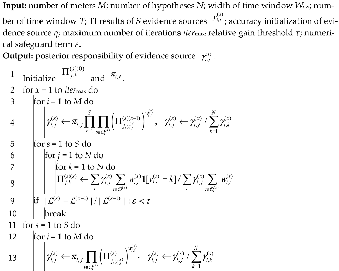3.2. Ca-TI Method Based on CCCG Enhanced D-S Evidence Fusion

During evidence fusion, conflicts among evidence sources are unavoidable. The classical Dempster rule filters the conflict mass through normalization and reallocates the remaining mass proportionally to competing hypotheses. As a result, when high conflict occurs, the fused outcome tends to be aggressive and may yield counter-intuitive results. By contrast, the classical Yager rule directly assigns the conflict mass to the uncertainty focal element, thereby avoiding forced decisions under high conflict. Consequently, the fusion outcome becomes more conservative and robust [35,36]. To balance information gain under low conflict and robustness under high conflict, this section exploits the complementarity between the Dempster and Yager rules and proposes an improved D-S fusion rule based on a conflict-gating mechanism.

3.2.1. Uncertainty-Aware BPA Construction

For D-S fusion, the meter-level posterior responsibilities are mapped to BPAs via uncertainty-aware mass assignment, and the resulting BPAs are further discounted considering the missing data rate.

In the uncertainty-aware mass assignment, the meter-level posterior responsibility is mapped to the BPA, with the posterior uncertainty controlling the reliability factor that trades off hypothesis masses against ignorance mass. The posterior uncertainty of evidence source s can be computed as follows:

$${\mathrm{conc}}_i^{(s)}=1-H({\gamma }_i^{(s)})/\log N,\hspace{1em}H\left({\gamma }_i^{(s)}\right)=-{\displaystyle \sum _{j=1}^N{\gamma }_{i,j}^{(s)}}\log \left({\gamma }_{i,j}^{(s)}\right)$$

(21)

where ${\mathrm{conc}}_i^{(s)}$ and ${\gamma }_i^{(s)}$ represent the posterior uncertainty and the posterior responsibility of the TI result for meter i from evidence source s; H(·) is the Shannon entropy function, and it is used to calculate the uncertainty of the posterior responsibility. The smaller the entropy value, the more concentrated the posterior responsibility becomes, indicating that the evidence source is more certain about the TI results for the meters. Conversely, it indicates that the evidence source finds it difficult to determine the TI results for the meters.

Due to missing data issues in LVDNs, time window data samples may be incomplete, potentially preventing evidence sources from performing TI. This may result in identification outcomes failing to meet subsequent evidence fusion requirements. Therefore, when calculating the BPA, the impact of missing data should be incorporated, as shown in the following equation:

$${\delta }_i^{(s)}=1-T_i^{(s)}/T,\hspace{1em}{T}_i^{(s)}={\displaystyle \sum _{t=1}^T{w}_{i,t}^{(s)}}1[y_{i,t}^{(s)}\ne \perp ]$$

(22)

where ${\delta }_i^{(s)}$ is the missing data rate in time windows of the TI for meter i by evidence source s; $T_i^{(s)}$ is the number of effective time windows for evidence source s to perform TI on meter i. According to the posterior uncertainty of the evidence source and the impact of the data quality, the BPA can be calculated as follows:

$$m_i^{(s)}(\{h_j\})=r_i^{(s)}{\gamma }_{i,j}^{(s)}, m_i^{(s)}({\Theta }_i)=1-r_i^{(s)}$$

(23)

$$r_i^{(s)}=G\left((1-{\delta }_i^{(s)})\cdot {\mathrm{conc}}_i^{(s)},0,1\right)$$

(24)

where $m_i^{(s)}(\{h_j\})$ denotes the BPA assigned by evidence source s to hypothesis $\{h_j\}$ for meter i; $m_i^{(s)}({\Theta }_i)$ denotes the BPA assigned by evidence source s to uncertainty for meter i, which is used to avoid overconfident identification by the evidence source when the posterior responsibility is not concentrated or when missing data are severe.$r_i^{(s)}$ is the reliability factor of evidence source s for the TI result of meter i; G(e, 0, 1) denotes the truncation function, which can restrict e to the interval [0, 1].

3.2.2. Improved D-S Evidence Fusion Rule Based on Conflict Gating

According to the BPA computation in Section 3.2.1, the conflict mass (C_i) among evidence sources for the TI result of meter i can be computed as follows:

$$C_i=1-{\displaystyle \prod _{s=1}^S{m}_i^{(s)}({\Theta }_i)}-{\displaystyle \sum _{j=1}^N\left[{\displaystyle \prod _{s=1}^S\left(m_i^{(s)}(\{h_j\})+m_i^{(s)}({\Theta }_i)\right)}-{\displaystyle \prod _{s=1}^S{m}_i^{(s)}({\Theta }_i)}\right]}$$

(25)

Then, the Dempster rule and the Yager rule are respectively used to obtain preliminary fusion BPAs for the TI result of meter i, as follows:

$$\begin{array}{l}{m}_{D,i}(\{h_j\})=\left[{\displaystyle \prod _{s=1}^S\left(m_i^{(s)}(\{h_j\})+m_i^{(s)}({\Theta }_i)\right)}-{\displaystyle \prod _{s=1}^S{m}_i^{(s)}({\Theta }_i)}\right]/\max (1-C_i,\epsilon )\\ m_{D,i}({\Theta }_i)={\displaystyle \prod _{s=1}^S{m}_i^{(s)}({\Theta }_i)}/\max (1-C_i,\epsilon )\end{array}$$

(26)

$$\begin{array}{l}{m}_{Y,i}(\{h_j\})={\displaystyle \prod _{s=1}^S\left(m_i^{(s)}(\{h_j\})+m_i^{(s)}({\Theta }_i)\right)}-{\displaystyle \prod _{s=1}^S{m}_i^{(s)}({\Theta }_i)}\\ m_{Y,i}({\Theta }_i)={\displaystyle \prod _{s=1}^S{m}_i^{(s)}({\Theta }_i)}+C_i\end{array}$$

(27)

where $m_{D,i}(•)$ and $m_{Y,i}(•)$ represent the preliminary fusion BPAs for the TI result of meter i based on the Dempster rule and Yager rule, respectively.

Further, a dynamic gating function is defined to construct the improved D-S fusion rule as follows:

$$g_i=\sigma \left(a(C_i-C_0)\right)$$

(28)

$$m_i(A)=(1-g_i)m_{D,i}(A)+g_i{m}_{Y,i}(A), A\in \{\{h_1\},\cdots ,\{h_N\},{\Theta }_i\}$$

(29)

where $m_i(A)$ represents the final fusion BPA for the TI of meter i based on the improved D-S fusion rule; g_i denotes the dynamic gating coefficient for fusing the TI result of meter i; $\sigma \left(•\right)$ is a sigmoid function satisfying $\sigma (x)=1/(1+e^{-x})$; a and C₀ represent the gating slope and gating threshold, respectively, both of which are hyperparameters of the dynamic gating function.

3.2.3. Computation of Dynamic Gating Hyperparameters

As shown in Section 3.2.2, the hyperparameters a and C₀ must be specified in advance, which introduces subjectivity. Therefore, this section establishes a hyperparameter calibration model based on consensus consistency among evidence sources. The model uses the Jousselme distance to measure the similarity between two sets of BPAs [36]. Specifically, the average Jousselme distance between the fused BPA and the BPAs of each evidence source is minimized as the objective function, with the lower and upper bounds of the hyperparameters as constraints. The mathematical formulation of the model is given as follows:

$$\begin{array}{l}\min f={\displaystyle \frac{1}{M}}{\displaystyle \sum _{i=1}^M\frac{1}{S}}{\displaystyle \sum _{s=1}^S{d}_J}\left({\mathit{M}}_i\left(a,C_0\right),{\mathit{M}}_i^{(s)}\right)\\ \mathrm{s}.\mathrm{t}.\left\{\begin{array}{l}{a}_{\min }\le a\le a_{\max }\hfill \\ 0\le C_0\le 1\hfill \end{array}\right.\end{array}$$

(30)

where $d_J\left(•,•\right)$ is the Jousselme distance metric function; ${\mathit{M}}_i\left(a,C_0\right)$ is the fusion BPA vector for the TI results of meter i satisfying ${\mathit{M}}_i\left(a,C_0\right)=\left[m_i(\{h_1\}),\cdots ,m_i(\{h_N\}),m_i({\Theta }_i)\right]$, and it is a function of the hyperparameters a and C₀. ${\mathit{M}}_i^{(s)}$ is the BPA vector of evidence source s for the TI result of meter i, satisfying ${\mathit{M}}_i^{(s)}=\left[m_i^{(s)}(\{h_1\}),\cdots ,m_i^{(s)}(\{h_N\}),m_i^{(s)}({\Theta }_i)\right]$. a_max and a_min represent the upper and lower limits of the gating slope (a), respectively.

3.2.4. Fusion Result Decision and Meter-Level Confidence Computation

According to the fusion BPA computed in Section 3.2.3, the pignistic function is used to compute the probability of each hypothesis. The final TI result of each meter is decided according to the maximum pignistic probability, as shown in Equation (31). The meter-level confidence is defined as the product of the informativeness and consistency, as shown in Equation (32). The fused uncertainty mass ($m_i({\Theta }_i)$) quantifies residual uncertainty due to insufficient evidence, while the conflict mass (C_i) quantifies inter-source contradiction. Hence, the confidence decreases when the evidence is either insufficient (high $m_i({\Theta }_i)$) or contradictory (high C_i), and it becomes high only when the evidence is both informative and consistent:

$${\widehat{y}}_i=\arg \underset{j}{\max }\left[m_i(\{h_j\})+m_i({\Theta }_i)/N\right]$$

(31)

$$con{f}_i=1-\left[\lambda m_i({\Theta }_i)+(1-\lambda )C_i\right]$$

(32)

where ${\widehat{y}}_i$ represents the final TI decision for meter i; $con{f}_i$ represents the meter-level confidence of the final TI result for meter i. λ is the weight coefficient.

The proposed Ca-TI method based on CCCG-DS evidence fusion is summarized in Algorithm 2.

Algorithm 2: Ca-TI Method Based on CCCG-DS Evidence Fusion

3.3. Overall Algorithm Procedure

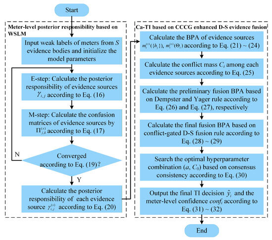
In summary, the overall procedure of the proposed method is shown in Figure 1.

Figure 1. Flow chart of proposed Ca-TI method for LVDNs.

4. Case Study

4.1. Case Descriptions

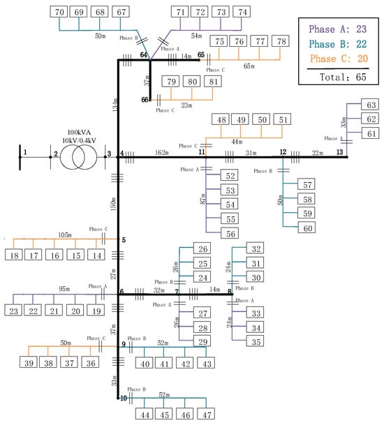
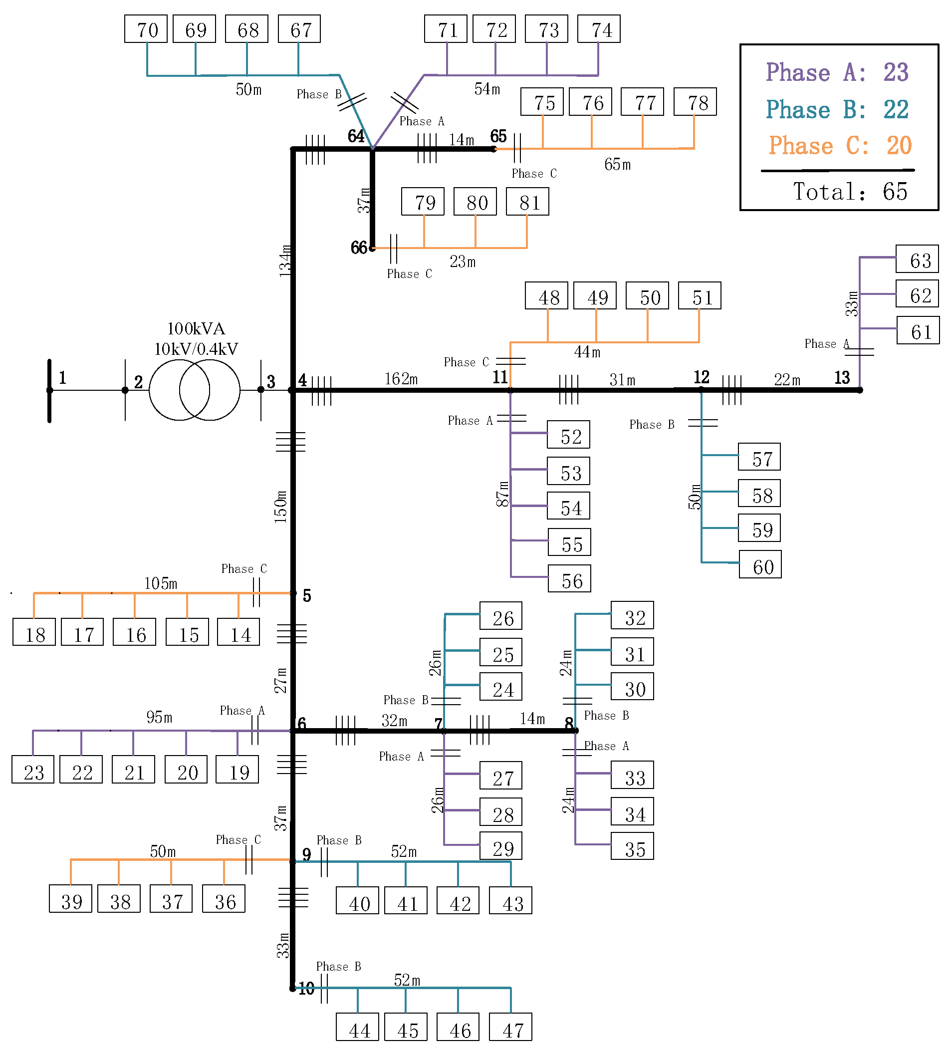
Case 1 (simulated LVDTA): A simulated LVDTA case is established, as shown in Figure 2. The LVDTA contains three low-voltage branches and 65 smart meters. The line models are set as follows: the main trunk line uses BLVV-150 × 4, and the meter service drop uses BLVV-50 × 2; line lengths are marked in the figure. The required voltage, current, and power data are obtained by three-phase four-wire power flow simulation for LVDNs [37]. The data sampling interval is 15 min, generating a total of 6 days of data, i.e., a data length of 576 points. To better match practical conditions, Gaussian noise with a mean of 0 and 3σ of 5% is added to the voltage and current curves obtained from the power flow calculation.

Figure 2. Topology structure of simulation substation in Case 1.

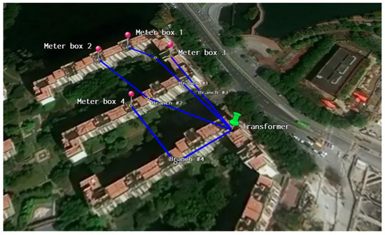
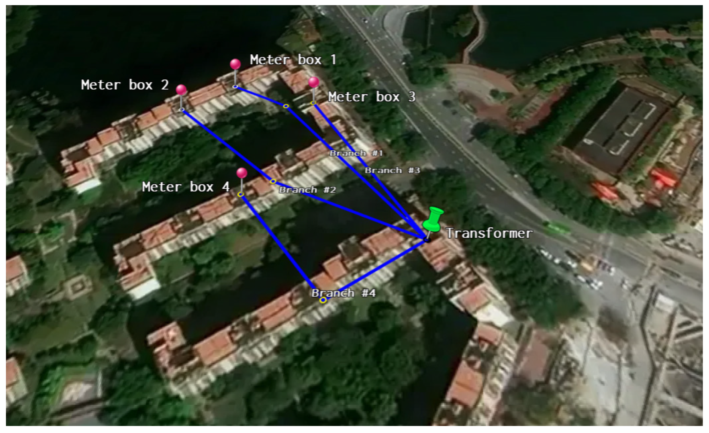
Case 2 (actual LVDTA): An actual LVDTA in Guangdong Province is selected for computational analysis, with its topology structure shown in Figure 3. This area is a typical urban residential service area, containing four low-voltage branches and 127 smart meters. For each meter, voltage, current, and power data are collected for 6 days, with a sampling interval of 15 min, i.e., a data length of 576 points.

Figure 3. Schematic diagram of actual substation in Case 2.

This paper uses C-PCI as an example for illustration. The identification methods proposed in References [13,16,18] are adopted as three evidence sources for fusion analysis and are defined as method 1, method 2, and method 3. The parameters of the algorithm are set in Table 2.

Table 2. Parameter setting of algorithm.

Parameter	Initial Value	Parameter	Initial Value
Number of hypotheses, N	3	Relative gain threshold of EM, τ	1 × 10−7
Width of time window, Wsw	288	Numerical safeguard term, ε	1 × 10−7
Sliding-window interval	1	Upper limit of gating slope, amax	50
Number of time windows, T	289	Lower limit of gating slope, amin	5
Accuracy initialization of evidence source, η	0.7	Weight coefficient, λ	0.5
Maximum number of iterations of EM, itermax	100	Confidence threshold, ϕ	0.8

To comprehensively evaluate both the overall identification performance and the decision reliability induced by confidence scores, three metrics are proposed, the overall accuracy (A_oa), high-confidence region accuracy (A_hc), and low-confidence error recall (R_lc), as shown in the following equations:

$$A_{\mathrm{oa}}={\displaystyle \sum _{i=1}^{M}1[{\widehat{y}}_i=y_i]}/M\times 100\%$$

(33)

$$A_{\mathrm{hc}}={\displaystyle \sum _{i\in \mathbf{\Omega }}1[{\widehat{y}}_i=y_i]}/\left|\mathbf{\Omega }\right|\times 100\%$$

(34)

$$R_{\mathrm{lc}}={\displaystyle \sum _{i\in \mathbf{\Psi }}1[{\widehat{y}}_i\ne y_i]}/\left|\mathbf{\Delta }\right|\times 100\%$$

(35)

where y_i is the ground-truth topology of meter i, and in the case study of this paper, it refers to the true C-PC label; Ω, Ψ are the high-confidence set and low-confidence set, respectively, satisfying $\mathbf{\Omega }=\left\{i|con{f}_i\ge \varphi \right\}$, $\mathbf{\Psi }=\left\{i|con{f}_i<\varphi \right\}$; Δ is the misidentification set, satisfying $\mathbf{\Delta }=\left\{i|{\widehat{y}}_i\ne y_i\right\}$.

4.2. Identification Procedure

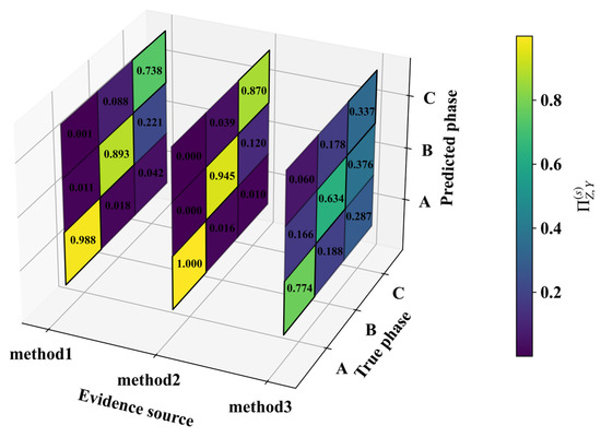
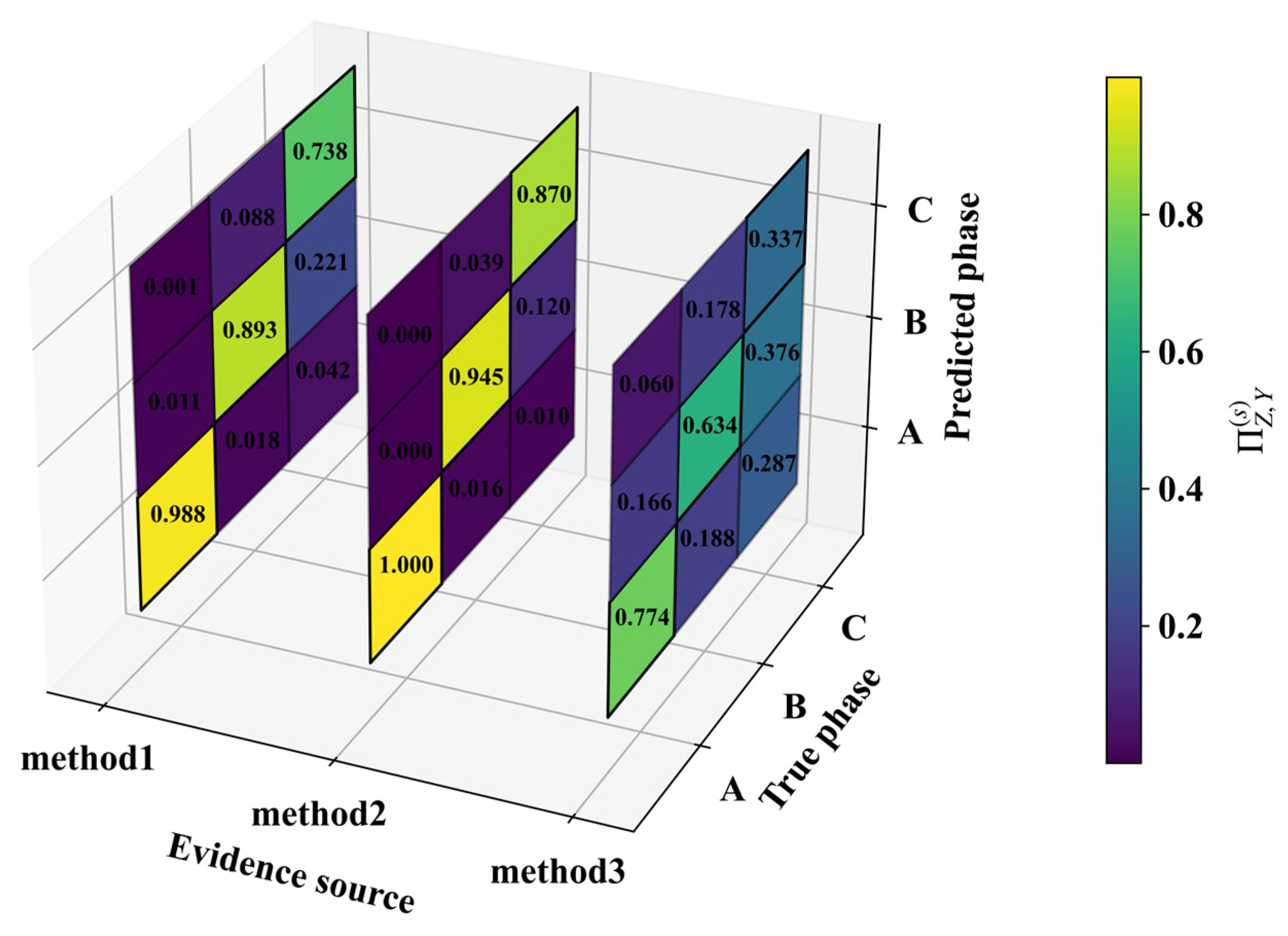
According to the WSLM proposed in this paper, the confusion matrices for method 1~method 3 can be calculated via the EM algorithm, as shown in Figure 4. In the confusion matrix, if the diagonal elements are large and close to 1, and the off-diagonal elements are small and close to 0, it indicates that the evidence source identification result has high stability; otherwise, it indicates randomness in the evidence source identification result. Specifically, the diagonal elements of the confusion matrices for method 1 (identifying Phase A and Phase B) and method 2 (for three-phase identification) are all greater than 0.85, indicating high stability, whereas method 3 corresponds to a confusion matrix where the diagonal elements are less than 0.8 (the diagonal elements of identifying Phase B and Phase C especially are significantly low, at only 0.634 and 0.337, respectively), indicating lower stability. According to the spatiotemporal characteristics of the consumer voltage analyzed in Reference [18], since the simulated LVDTA has small three-phase voltage unbalance, short supply lines, and light load levels, the voltage differences among meters are small. Method 3 is essentially based on voltage correlation for C-PC, which easily leads to significant randomness in identification results. It is evident that the reliability of identification results from a single method alone is difficult to guarantee. Through the proposed WSLM, fusion evaluation among multiple methods can be achieved, and the qualitative observation of the reliability of each method’s identification results can be realized without ground-truth topology labels.

Figure 4. Confusion matrices of three evidence sources.

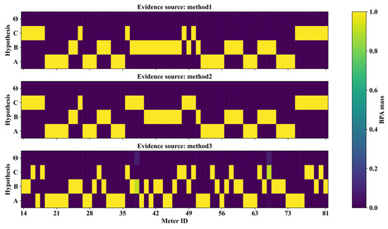
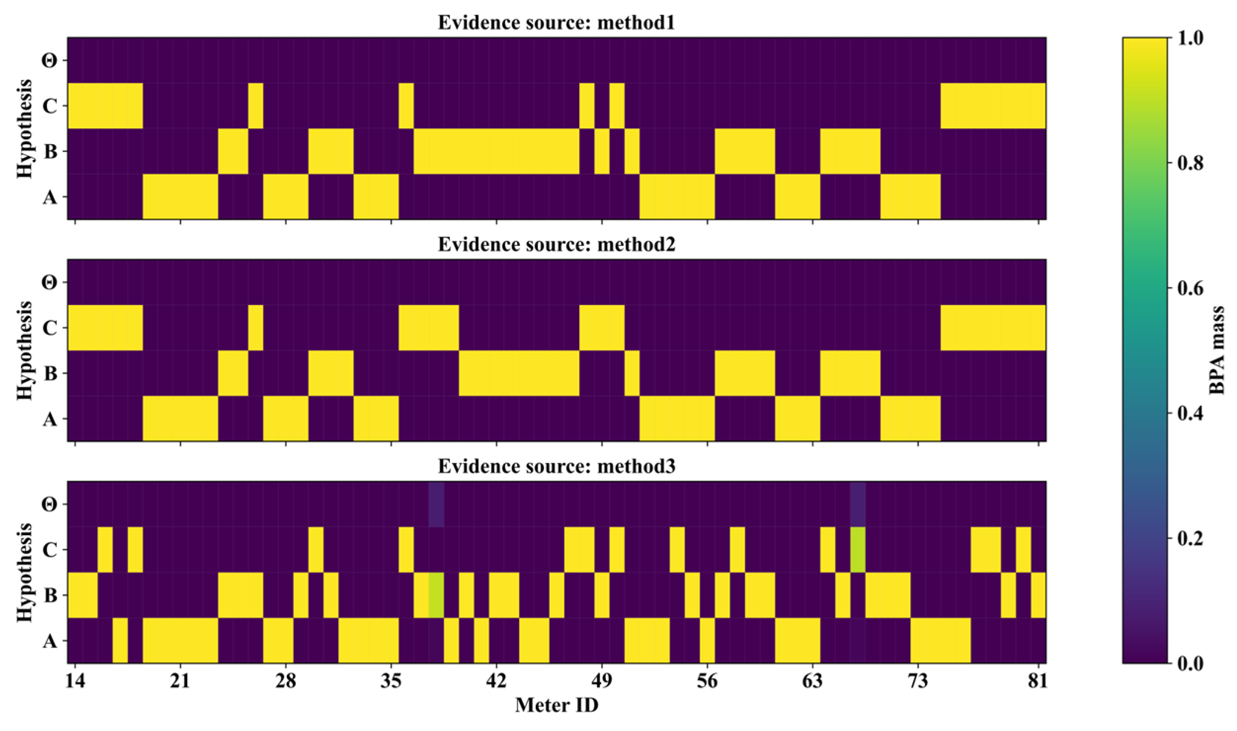
The posterior responsibilities of each evidence source are iteratively inferred using the EM algorithm until convergence. According to Equations (21)–(24), the BPA of each hypothesis for the C-PCI of each meter can be calculated, as shown in Figure 5. It can be seen that: (1) Method 1 and method 2 have high identification certainty. The identification result of each meter is assigned to a specific phase with a high probability value. (2) In contrast, method 3 shows randomness in the identification results, and the phase assignment for some meters is uncertain. Moreover, it can be intuitively observed that although various methods yield highly confident identification results for certain meters, the C-PCI labels differ and conflict with one another. Consequently, it is impossible to determine which result should ultimately be trusted.

Figure 5. BPA of C-PCI hypotheses for each meter based on three evidence sources.

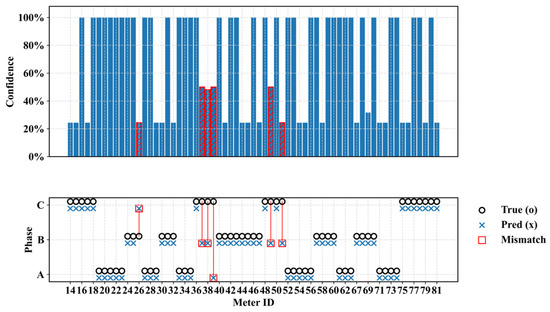
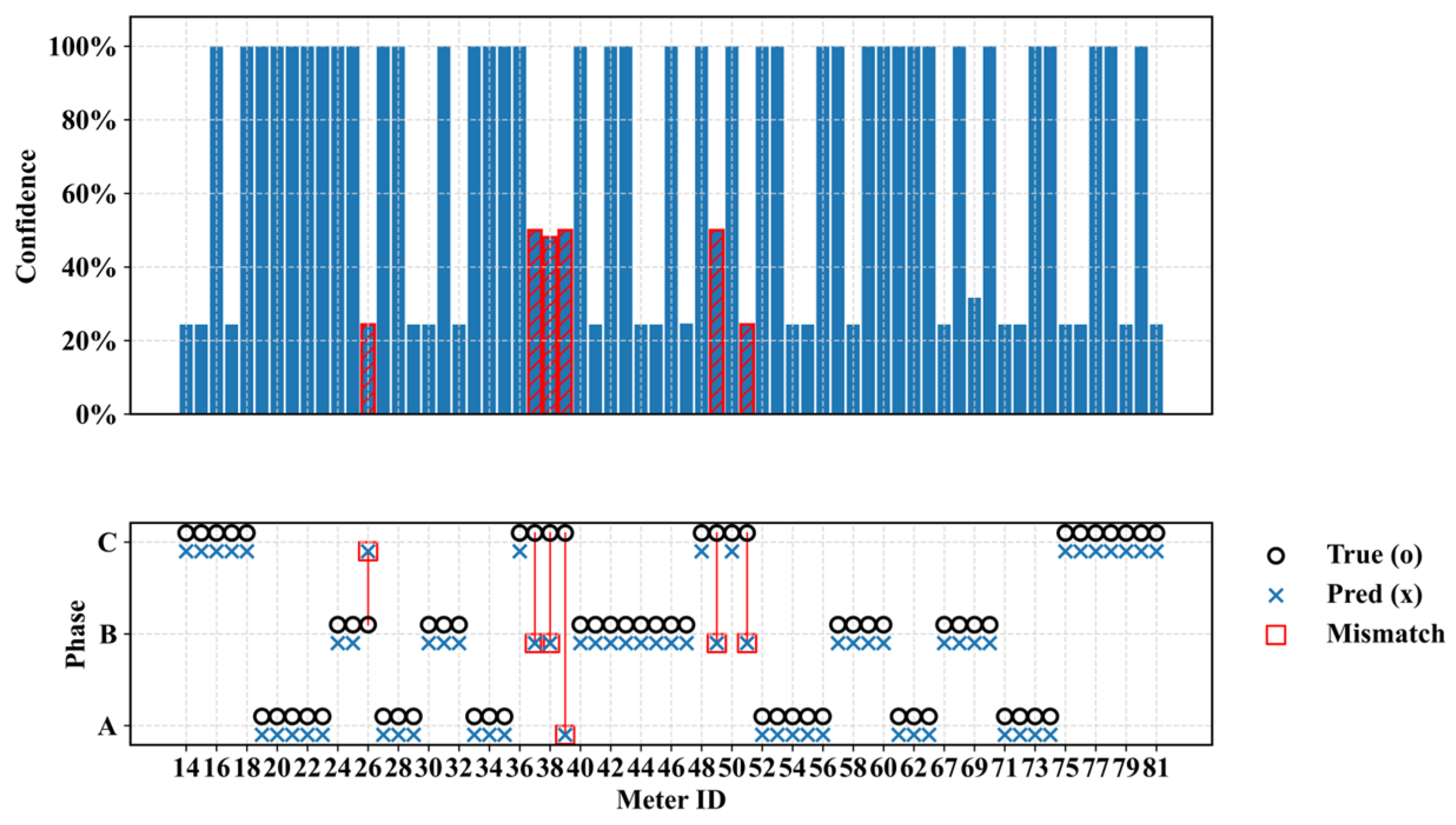
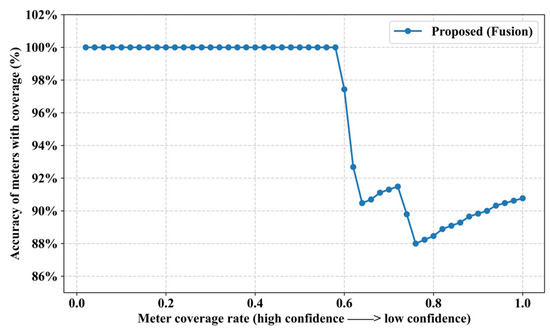
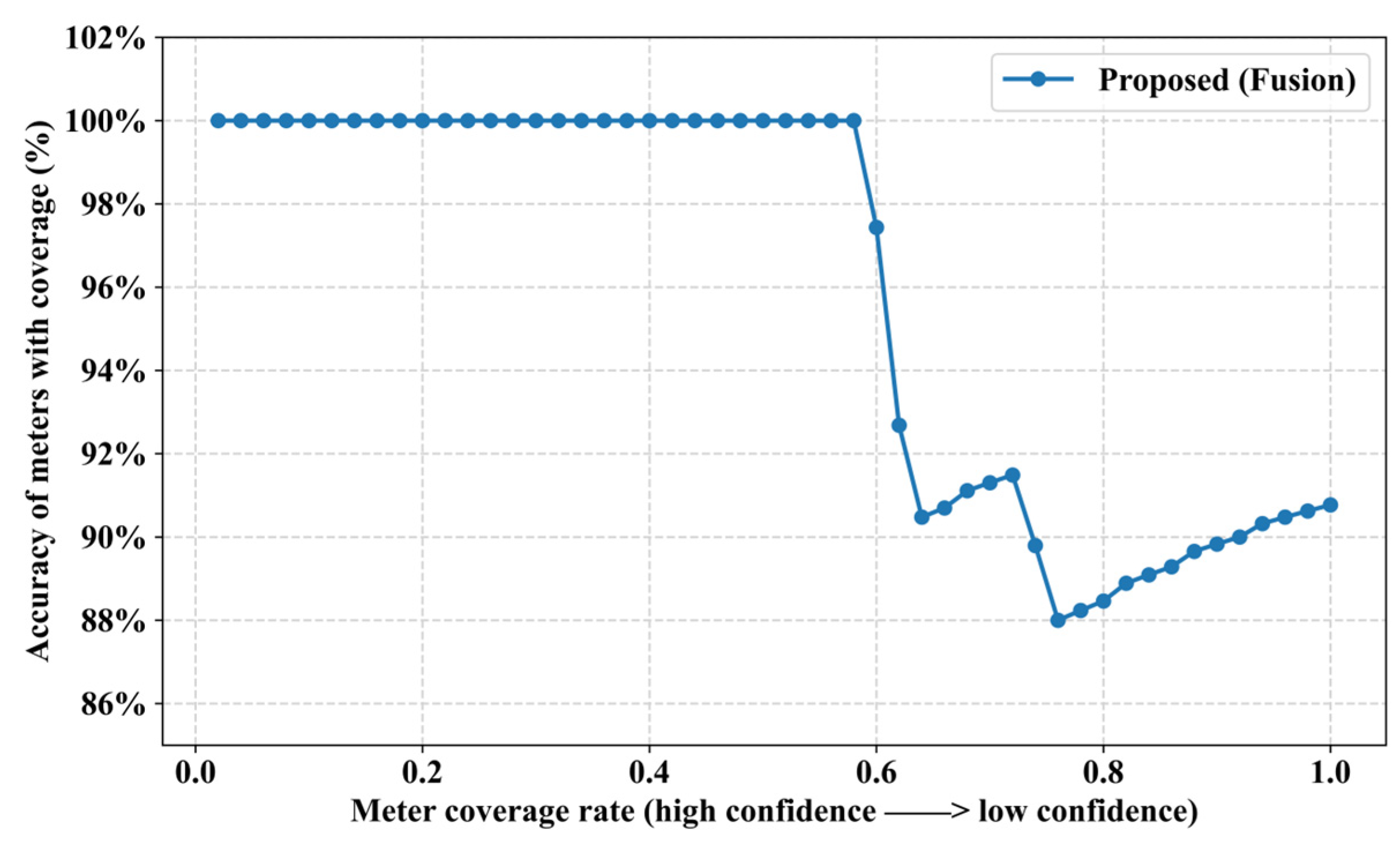
Furthermore, the proposed CCCG-DS evidence fusion method was used to fuse the identification results of the three evidence sources, and the fusion results are shown in Figure 6. Compared with the true phase labels, the relationship curve between the accuracy of meters with coverage and the meter coverage rate can be output, as shown in Figure 7. The x-axis represents the coverage statistics obtained by ranking meters in descending order of confidence scores. And the overall accuracy (A_oa), high-confidence region accuracy (A_hc), and low-confidence error recall (R_lc) are calculated as shown in Table 3. According to Figure 6 and Figure 7 and Table 3, it can be seen that the fusion method achieved results consistent with method 1, with an overall accuracy (A_oa) of 90.77%, and it improved by −6.35% and 51.28% compared with method 2 and method 3, respectively; the fusion method can effectively integrate the performances of various identification methods, and it is not adversely affected by extreme bias from any single method (such as method 3). Moreover, the fusion method can provide meter-level confidence. And when the confidence threshold (ϕ) is set as 0.8, the high-confidence region accuracy (A_hc) and the low-confidence error recall (R_lc) can achieve 100%. This means that the fusion result for the meters in the high-confidence set (Ω) can be trusted, and only the meters in the low-confidence set (Ψ) should be on-site-verified, which can significantly reduce the on-site verification work.

Figure 6. Results of C-PCI and confidence based on proposed fusion method in Case 1.

Figure 7. Curve of meters with coverage to accuracy based on proposed fusion method.

Table 3. Performance comparison of methods 1/2/3 and proposed method in Case 1.

Method	Aoa	Ahc	Rlc
Method 1	90.77%	/	/
Method 2	96.92%	/	/
Method 3	60.00%	/	/
Proposed method	90.77%	100%	100%

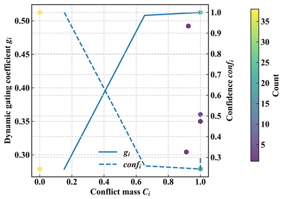
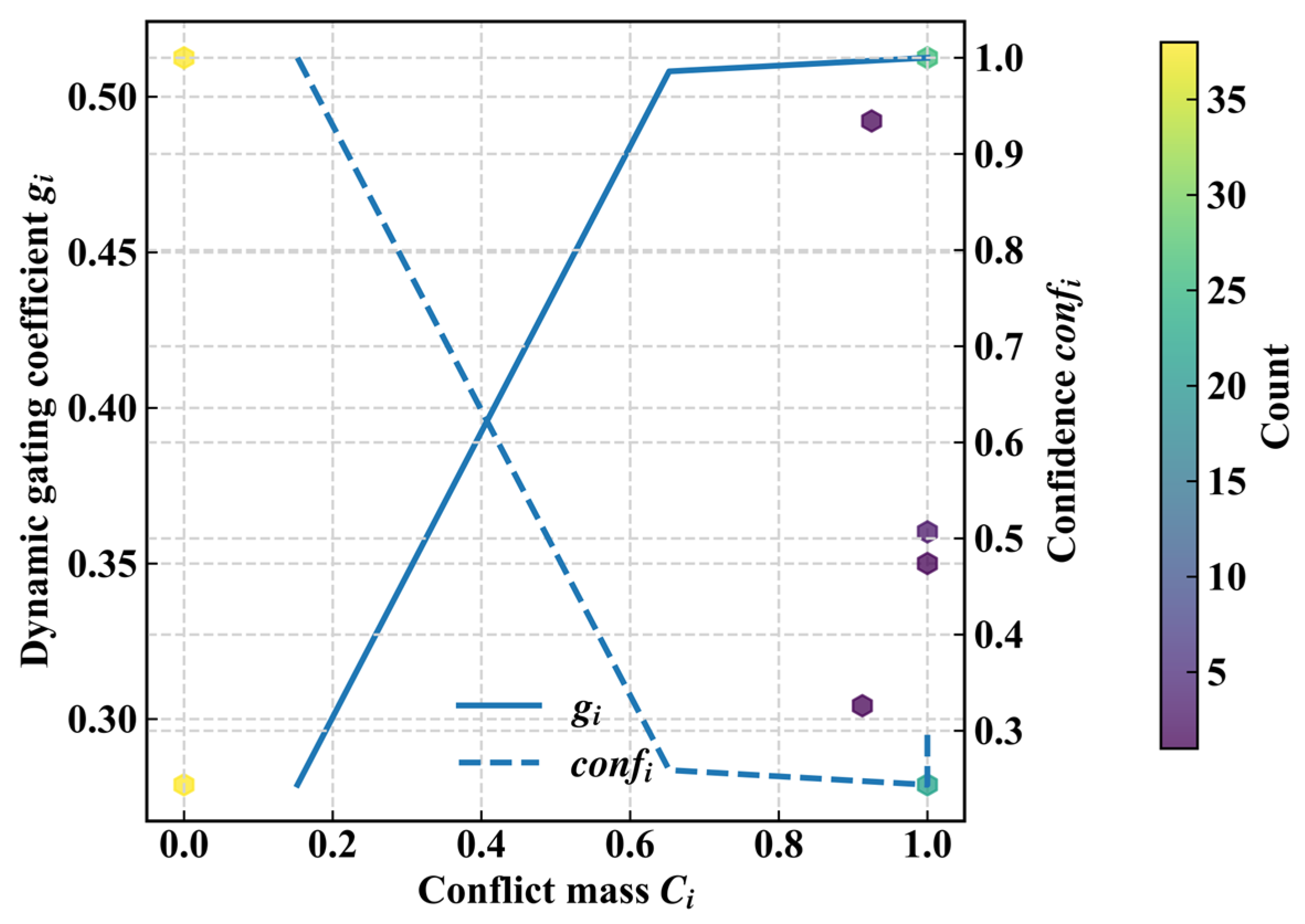
To further explain the high accuracy performance of the fusion method, Figure 8 provides the relationship curves for the dynamic gating coefficient, confidence score and conflict mass. It can be intuitively observed that as the confidence score decreases, the conflict mass increases, and the dynamic gating coefficient gradually increases. For identification results with high conflict, the proposed conflict-gating mechanism can bias them towards the Yager rule, thereby avoiding forced judgment and decision bias under high conflict, making the fusion result more robust. For meters with high conflict, the proposed method can effectively assign them to the low-confidence region. This can effectively reduce the deviation caused by the overconfidence of a certain single method, and it can effectively distinguish between high-confidence and low-confidence meter regions, helping to guide targeted and efficient on-site operation and maintenance.

Figure 8. Curve of conflict mass to dynamic gating coefficient and confidence.

4.3. Effectiveness Verification of Proposed Algorithm

4.3.1. Verification of Proposed WLSM

To verify the effectiveness of the WSLM in learning source error patterns without ground-truth labels, and to quantify its contribution to downstream fusion performance, two comparison scenarios are set as follows (to isolate the effect of the CCCG-DS fusion method, the fusion rule is fixed to Dempster-only, and only the presence/absence of the WSLM is compared):

Scenario 1: WSLM + Dempster-only fusion: The WSLM is trained via EM using multi-source outputs to estimate source confusion matrices. And BPAs are constructed, followed by Dempster’s combination rule to obtain the fused prediction.

Scenario 2: No-WSLM + Dempster-only fusion: The WSLM is disabled, and no confusion matrix is learned. For each source, $m_i^{(s)}(\{h_j\})$ is obtained by frequency counting across windows [18], and $m_i^{(s)}({\Theta }_i)$ is set as zero, followed by the same Dempster-only fusion.

Since the proposed CCCG-DS fusion method was not adopted, the meter-level confidence could not be calculated. So, only the overall accuracy (A_oa) was used for the performance comparison of two scenarios. To mitigate the random effects of Gaussian noise, we repeated the experiment 100 times and calculated the expectation (exp) and standard deviation (std) of the evaluation metrics. The results are shown in Table 4. Compared with Scenario 2, enabling the WSLM increased the exp of A_oa from 91.29% to 98.71% and decreased the std of A_oa from 5.12% to 1.71%. This demonstrates that the WSLM can effectively learn each source’s error pattern from multi-source consensus without ground-truth labels, thereby improving the evidence construction and mitigating the adverse impact of unreliable sources in fusion. Consequently, the WSLM constitutes a critical component of the proposed framework rather than a classical frequency-counting strategy.

Table 4. Performance comparison of Scenario 1 and Scenario 2.

Scenario	Aoa
	exp	std
Scenario 1	98.71%	1.71%
Scenario 2	91.29%	5.12%

4.3.2. Verification of Proposed CCCG-DS Fusion

To verify the effectiveness of the CCCG-enhanced D-S evidence fusion method proposed in Section 3.2, five comparison scenarios are set, as described in Table 5. It should be noted that the voting-based fusion method [25] and the WSLM without fusion cannot provide meter-level confidence. To better compare the performances of the methods in various scenarios, the maximum value of frequency statistics was used to approximate the confidence for the voting-based fusion method, and the maximum posterior responsibility was used to approximate the confidence for the WSLM without fusion. Similarly, we repeated the experiments 100 times and calculated the exp and std of the evaluation metrics. The evaluate metrics for each scenario are shown in Table 6.

Table 5. Comparison scenario setting.

Scenario	Description
Scenario 3	Voting-based fusion [25]
Scenario 4	WSLM only (without fusion)
Scenario 5	WSLM + Dempster-only fusion
Scenario 6	WSLM + Yager-only fusion
Scenario 7	Proposed method (WSLM + CCCG-DS fusion)

Table 6. Performance comparison of Scenario 3–Scenario 7.

Scenario	Aoa		Ahc		Rlc
	exp	std	exp	std	exp	std
Scenario 3	94.77%	3.46%	95.41%	3.31%	12.31%	19.25%
Scenario 4	98.71%	1.71%	98.71%	1.71%	0%	0%
Scenario 5	98.71%	1.71%	99.73%	0.74%	84.52%	33.00%
Scenario 6	98.49%	1.72%	99.72%	0.75%	87.63%	28.21%
Scenario 7	98.58%	1.70%	99.73%	0.74%	86.02%	31.65%

According to Table 5, the results show that:

(1)

The WSLM only in Scenario 4 achieved a comparable overall accuracy to that of the fusion-informed methods in Scenario 5~Scenario 7. However, R_lc of the WSLM-only scenario is 0, which indicates that erroneous meters were not flagged as low-confidence for inspection, and A_hc degenerated to A_oa (98.71% ± 1.71%). In contrast, the fusion-informed methods preserved high A_oa while substantially improving error triage. For example, WSLM + CCCG-DS fusion achieved high A_oa (98.58% ± 1.70%) and high A_hc (99.73% ± 0.74%) and significantly higher error recall in the low-confidence region (86.02% ± 31.65%). Therefore, the advantage and necessity of informed fusion are not tied to a monotonic improvement in A_oa but rather to providing an interpretable conflict-aware confidence that enables targeted verification for low-confidence meters, thereby reducing unnecessary field checks.

(2)

Comparing CCCG-DS fusion against Dempster-only fusion and Yager-only fusion can further validate the effectiveness of the CCCG mechanism. Their A_oa and A_hc are all high and close. Yet, CCCG exhibits a more balanced risk behavior: its R_lc lies between the other two rules, indicating that sample-wise gating adaptively trades off between Dempster’s more aggressive normalization and Yager’s more conservative conflict absorption, yielding a more even trade-off between high-confidence meters without verification and low-confidence meters with error recall.

(3)

The voting-based fusion method achieved relatively high A_oa and high A_hc. However, its R_lc performed significantly poorer than the proposed method, indicating that the voting mechanism based on superficial agreement does not reliably flag misidentified meters. The proposed method in this paper can mine the identification consensus among multiple sources and assign high and low probabilities to decisions for identification consensus and difference, respectively, which better supports a practical deployment for “trust and verification”.

4.4. Robustness Testing

To further verify the robustness of the proposed method, various scenarios involving measurement noise and missing data were set, and the methods set in Table 4 were tested. Specifically, for the analysis of the measurement noise impact, Gaussian noise with a mean of 0 and 3σ of 0%, 5%, 10%, 15% and 20% was added to the voltage and current curves without missing data; for the analysis of the missing data impact, missing data rates of 0%, 5%, 10%, 15% and 20% were simulated with 5% measurement noise. The evaluation metrics for each method are shown in Table 7 and Table 8.

Table 7. Performances of methods under different measurement noise levels.

Scenario	Measurement Noise	Aoa		Ahc		Rlc
		exp	std	exp	std	exp	std
Scenario 3	0%	100%	0	100%	0	/	/
Scenario 4		100%	0	100%	0	/	/
Scenario 5		100%	0	100%	0	/	/
Scenario 6		100%	0	100%	0	/	/
Scenario 7		100%	0	100%	0	/	/
Scenario 3	5%	94.77%	3.46%	95.41%	3.31%	12.31%	19.25%
Scenario 4		98.71%	1.71%	98.71%	1.71%	0%	0%
Scenario 5		98.71%	1.71%	99.73%	0.74%	84.52%	33.00%
Scenario 6		98.49%	1.72%	99.72%	0.75%	87.63%	28.21%
Scenario 7		98.58%	1.70%	99.73%	0.74%	86.02%	31.65%
Scenario 3	10%	81.29%	5.19%	82.36%	5.05%	8.93%	8.33%
Scenario 4		94.92%	3.39%	94.92%	3.39%	0%	0%
Scenario 5		92.34%	3.37%	97.61%	3.05%	86.56%	19.15%
Scenario 6		87.85%	4.85%	97.58%	3.09%	90.67%	14.12%
Scenario 7		89.94%	4.02%	97.60%	3.08%	89.30%	17.09%
Scenario 3	15%	73.82%	6.03%	74.78%	6.10%	7.73%	7.08%
Scenario 4		90.89%	4.36%	90.89%	4.36%	0%	0%
Scenario 5		86.31%	3.93%	94.55%	4.40%	86.97%	11.49%
Scenario 6		77.97%	4.99%	94.83%	4.65%	92.17%	7.36%
Scenario 7		82.37%	4.15%	94.62%	4.35%	90.02%	8.79%
Scenario 3	20%	70.77%	5.00%	71.85%	4.89%	7.37%	5.79%
Scenario 4		86.58%	8.73%	86.58%	8.73%	0%	0%
Scenario 5		82.71%	9.15%	91.81%	10.13%	85.25%	12.33%
Scenario 6		73.66%	7.79%	91.76%	10.34%	90.29%	8.78%
Scenario 7		77.94%	8.79%	91.84%	10.15%	88.28%	10.49%

Table 8. Performances of methods under different missing data rates.

Scenario	Missing Data	Aoa		Ahc		Rlc
		exp	std	exp	std	exp	std
Scenario 3	0%	94.77%	3.46%	95.41%	3.31%	12.31%	19.25%
Scenario 4		98.71%	1.71%	98.71%	1.71%	0%	0%
Scenario 5		98.71%	1.71%	99.73%	0.74%	84.52%	33.00%
Scenario 6		98.49%	1.72%	99.72%	0.75%	87.63%	28.21%
Scenario 7		98.58%	1.70%	99.73%	0.74%	86.02%	31.65%
Scenario 3	5%	86.24%	3.97%	87.58%	4.02%	9.86%	11.37%
Scenario 4		96.85%	2.68%	96.85%	2.68%	0%	0%
Scenario 5		94.52%	2.84%	97.93%	2.79%	84.76%	23.05%
Scenario 6		91.21%	2.69%	97.88%	2.65%	86.55%	19.63%
Scenario 7		92.78%	2.75%	97.90%	2.72%	85.22%	21.54%
Scenario 3	10%	80.86%	4.83%	82.02%	4.78%	8.52%	10.01%
Scenario 4		94.69%	3.42%	94.69%	3.42%	0%	0%
Scenario 5		90.78%	3.71%	95.66%	3.79%	86.42%	19.90%
Scenario 6		87.40%	3.65%	95.89%	3.68%	88.76%	17.28%
Scenario 7		88.89%	3.70%	95.85%	3.66%	87.59%	18.79%
Scenario 3	15%	75.24%	5.69%	76.83%	5.80%	7.22%	7.54%
Scenario 4		92.36%	4.67%	92.36%	4.67%	0%	0%
Scenario 5		86.63%	4.92%	93.26%	4.88%	87.30%	17.75%
Scenario 6		83.22%	4.80%	92.92%	4.83%	89.84%	15.17%
Scenario 7		84.51%	4.86%	93.03%	4.79%	88.38%	16.56%
Scenario 3	20%	71.35%	5.88%	72.75%	5.69%	7.01%	6.85%
Scenario 4		89.83%	5.52%	89.83%	5.52%	0%	0%
Scenario 5		82.45%	7.92%	90.94%	8.11%	88.46%	15.37%
Scenario 6		78.81%	7.10%	90.44%	8.36%	90.79%	12.99%
Scenario 7		81.06%	7.55%	90.75%	8.20%	89.54%	14.24%

According to Table 7, as the noise level increases from 5% to 20%, all methods exhibit a monotonic drop in each evaluation metric, accompanied by noticeably larger standard deviations. However, the proposed method (WSLM + CCCG-DS fusion) remains advantageous because its R_lc stays consistently high and relatively stable across all noise levels. This indicates that even under stronger noise, the proposed method can still concentrate most misidentified meters into the low-confidence region, enabling targeted on-site verification. In contrast, the voting-based method suffers a sharper accuracy decline (A_oa and A_hc) while keeping a persistently low and further decreasing R_lc, implying that superficial agreement alone is insufficient for robust identification.

Moreover, comparing the other fusion methods in Scenario 5 and Scenario 6, it can be observed that WSLM + Dempster-only fusion performs better on A_oa and A_hc, whereas WSLM + Yager-only fusion performs better on R_lc. This further indicates that Dempster’s rule is more decisive, while Yager’s rule is more conservative, and that the proposed method can achieve an effective balance, ensuring robustness against the measurement noise.

According to Table 8, the overall impact pattern of missing data is similar to that of measurement noise. The proposed method remains advantageous under heavier missingness: by learning source-specific error patterns in a weakly supervised manner and applying conflict-gated fusion, it explicitly characterizes the insufficient evidence and conflicting evidence, enabling the low-confidence region more stably. This yields a more robust and verifiable decision behavior under adverse data conditions, highlighting its robustness for practical deployment.

4.5. Sensitivity Analysis of Preset Thresholds

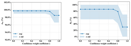
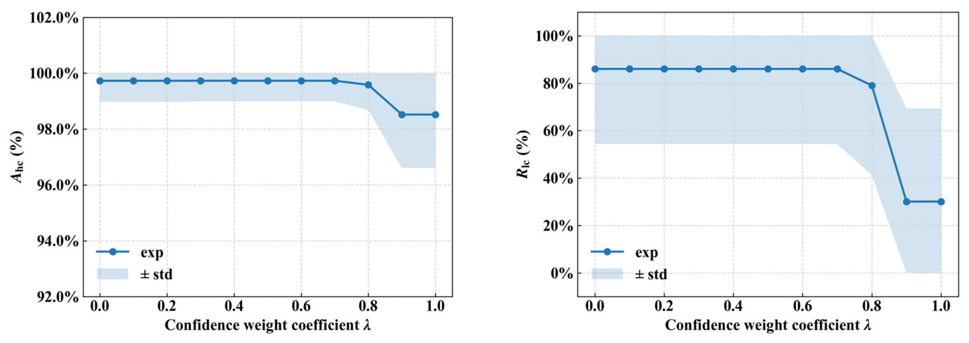
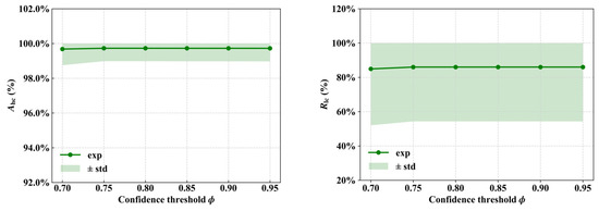
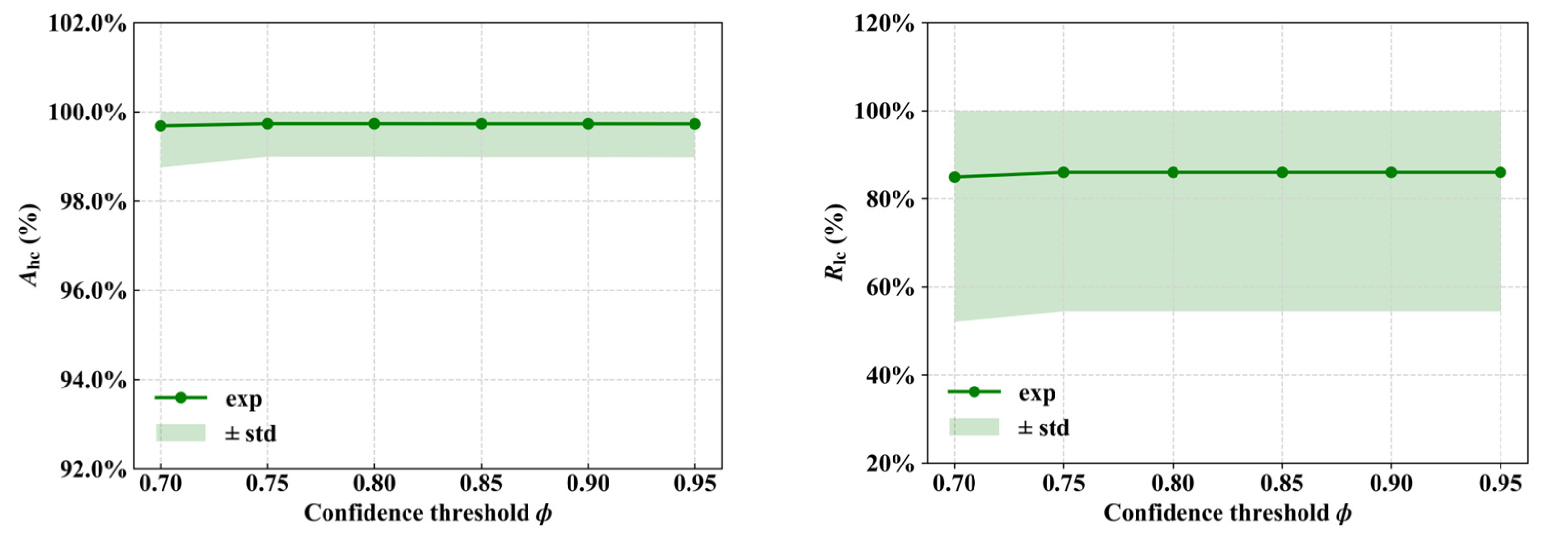
The proposed method involves several preset thresholds, and a sensitivity analysis of these parameters is required. The main preset thresholds are listed in Table 2. Except for the weight coefficient (λ) of the meter-level confidence calculation and the confidence threshold (ϕ) of the evaluation metrics, the other thresholds are not decision-critical. They mainly ensure numerical stability and do not change the predicted labels, such as τ, ε, η, and iter_max. And the hyperparameters a and C₀ of CCCG-DS fusion are adaptively learned rather than manually tuned. Thus, the sensitivity analysis of λ and ϕ was carried out. Gaussian noise with a mean of 0 and 3σ of 5% was added to the voltage and current curves without missing data. The experiment was repeated 100 times, and the exp and std of A_hc and R_lc were calculated. The results are shown in Figure 9 and Figure 10.

Figure 9. Exp and std of A_hc and R_lc under different weight coefficients (λ).

Figure 10. Exp and std of A_hc and R_lc under different confidence thresholds (ϕ).

According to Figure 9, the result shows that A_hc and R_lc both remain stable when λ is in the low-to-medium range (e.g., 0 ≤ λ ≤ 0.7) but degrades sharply when λ becomes large. This degradation is expected because overly weighting the uncertainty term effectively downplays the conflict component in the confidence computation, making source disagreement less likely to be reflected as low-confidence risk. Therefore, we recommend choosing λ in a moderate-to-low range to obtain robust confidence partitioning and reliable error control.

According to Figure 10, the result shows that the variation in λ has a minor impact on A_hc and R_lc, with both remaining largely stable, indicating that the proposed method is insensitive to λ and provides consistent high-confidence decisions and error recall.

4.6. Validation Based on Actual LVDTA

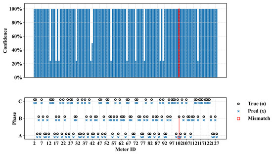
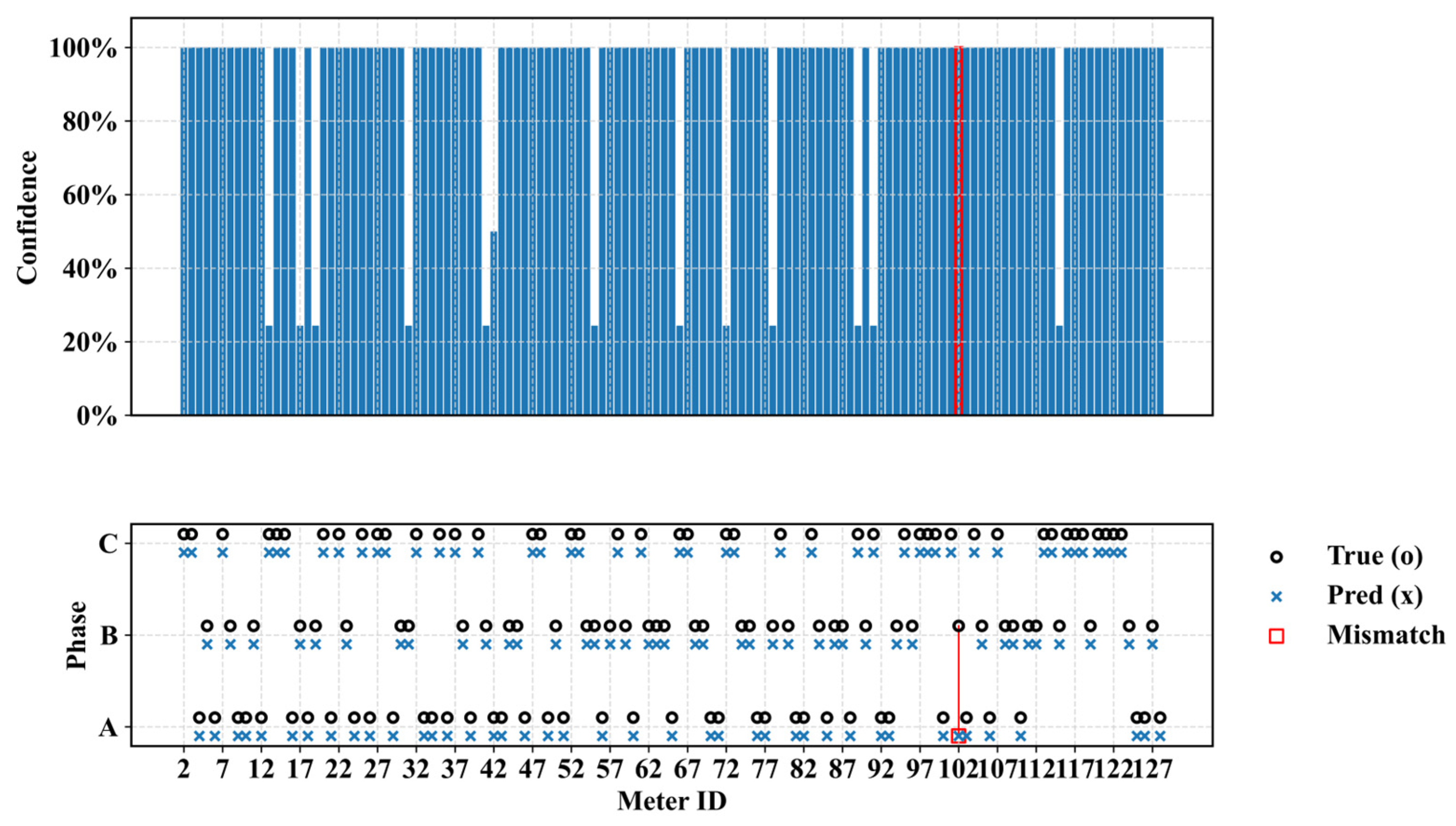
To further verify the applicability of the proposed method in practical scenarios, a performance comparison analysis between single methods and the fusion method was carried out based on the actual LVDTA in Case 2. The identification results of the fusion method proposed are shown in Figure 11, and the performance comparison of the three single methods and the proposed fusion method is shown in Table 9.

Figure 11. Results of C-PCI and confidence based on proposed fusion method in Case 2.

Table 9. Performance comparison of methods 1/2/3 and proposed method in Case 2.

Method	Aoa	Ahc	Rlc
Method 1	99.21%	/	/
Method 2	91.34%	/	/
Method 3	54.33%	/	/
Proposed method	99.21%	99.21%	0%

According to Table 8, the result shows that the A_oa of a single method varies in different cases. For example, method 2 performed the best in Case 1, whereas method 2 performed the best in Case 2. So, relying on a single method cannot guarantee stable accuracy. The proposed fusion method is not adversely affected by extreme bias from any single method and is able to maintain high identification accuracy. However, R_lc equals 0% mainly because the total number of misidentified meters is extremely small (only one error in this case) and the misidentified meter is assigned to the high-confidence set. This typically happens when sources exhibit consistent, correlated errors, leading to low uncertainty mass and low conflict, thus resulting in high confidence despite the incorrect prediction. Therefore, this reflects the challenge of detecting errors in correlated multi-source scenarios, which creates the need for future work.

5. Further Discussion on Engineering Deployment with Cloud–Edge Collaboration

5.1. Analysis of Mainstream LVDN TI Methods

The mainstream methods for LVDN TI can be broadly categorized into three types: the signal injection-based method, BPLC-based method and data driven-based method. The case study in Section 4 is analyzed based on the data driven-based method but is also applicable to the signal injection-based method and BPLC-based method. However, different types of identification methods differ in their characteristics and application scenarios and using only one type of method can hardly satisfy practical application requirements. The characteristics of these methods are summarized in Table 10. In the “Identification Ability” column, ”√” indicates that the method only supports the identification of the meters registered in the metering archives. It cannot identify the meters that are actually supplied by the local LVDTA but not included in the metering archives. ”√√” indicates that the method supports the identification of the meters registered in the metering archives. After data analysis in the cloud platform, the meters that are actually supplied by the local LVDTA but not listed in the archive can be identified.

Table 10. Summary of characteristics of mainstream LVDN TI methods.

Method	Application Requirement	Identification Ability	Deployment Location
Signal injection-based method	High configuration LVDTAs with characteristic signal modules and BPLC communication module equipment	√ C-TCI √ C-PCI √ C-BCI	× Cloud √ Edge
BPLC-based method	Standard configuration LVDTAs with BPLC communication module equipment	√ C-TCI √ C-PCI × C-BCI	× Cloud √ Edge
Data driven-based method	Other LVDTAs without characteristic signal modules and BPLC communication module equipment	√√ C-TCI √√ C-PCI √√ C-BCI	√ Cloud √ Edge

Note: “√” indicates that the method only supports to identify the meters registered in the metering archives. It cannot identify the meters that are actually supplied by the local LVDTA but not included in the metering archives. “√√” indicates that the method supports to identify the meters registered in the metering archives. “×” indicates that the method is unable to identify.

According to Table 10: (1) In terms of application requirements, the signal injection-based method is the most demanding, requiring that devices such as transformer terminal units, branch terminal units and smart meters in the LVDTA be equipped with characteristic signal modules. The BPLC-based method is less demanding. With the continuous maturation of BPLC technologies, the local communication schemes in LVDTAs are being progressively upgraded to BPLC; therefore, standard configuration LVDTAs can generally support the BPLC-based method. The data driven-based method has the lowest requirements. Under the AMI, the measurement data in the LVDTA can be collected, and the data driven-based method can be carried out without characteristic signal modules and BPLC communication modules. (2) In terms of the identification ability and deployment location, because the signals monitored by the signal injection-based method and BPLC-based method are high-frequency and cannot be frequently reported to the cloud platform, these two types of methods can only be deployed on the edge side. Moreover, they can only identify meters included in the metering archives on the edge side. When there exist meters that are actually supplied by the target LVDTA but not included in the metering archives, these two methods do not support it. By contrast, the data driven-based method can be deployed either on the cloud side or on the edge side. In addition, measurement data from the LVDTA can be reported to the cloud platform to carry out the cross-LVDTA identification, achieving identification of the complete topology for the LVDTA.

5.2. Engineering Deployment Architecture

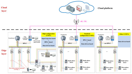
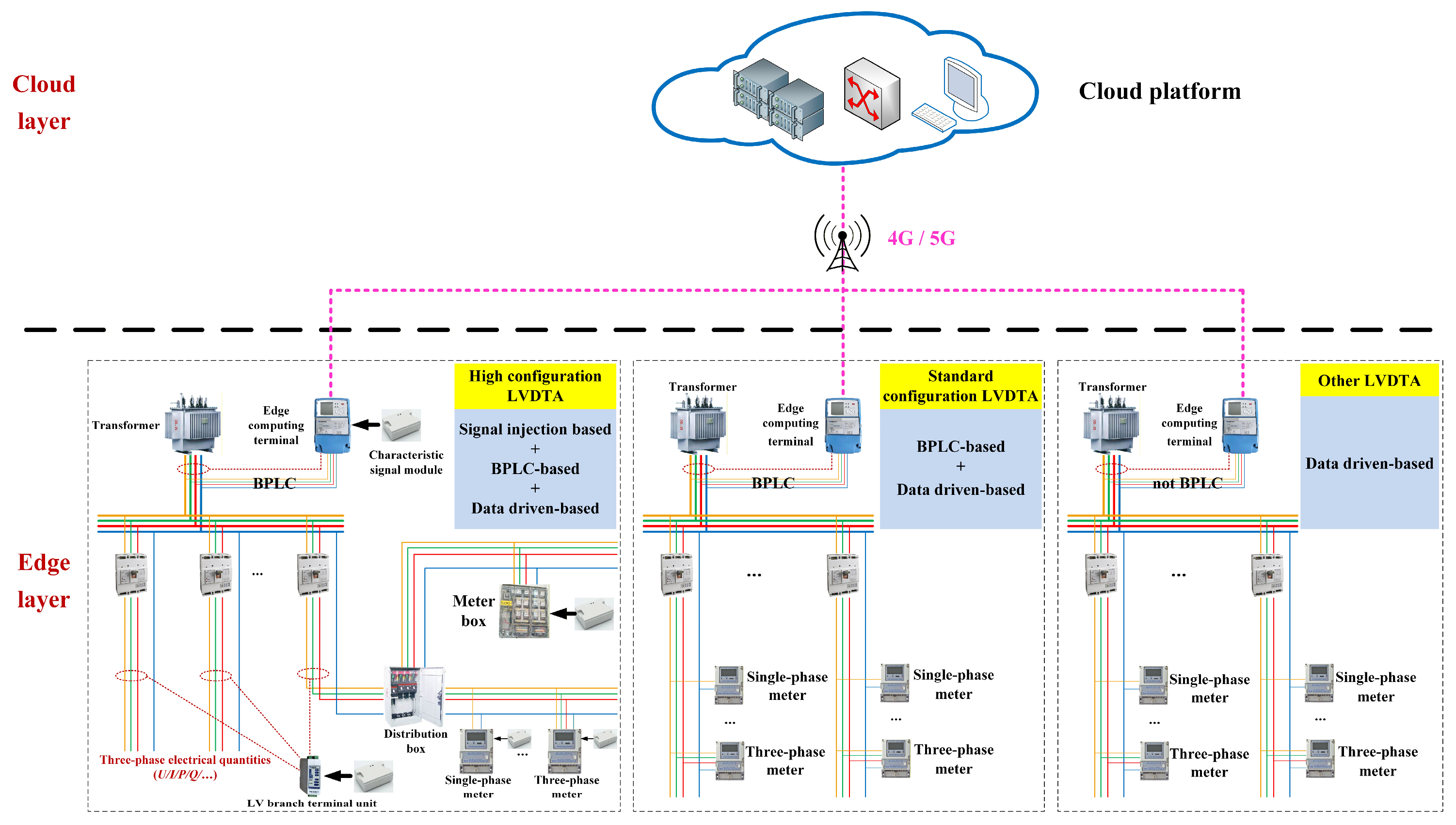
Based on the cloud–edge collaboration framework of the PIoT, a system architecture for LVDN TI applications is designed, as shown in Figure 12.

Figure 12. System architecture of topology identification for LVDN.

Edge layer: This mainly refers to edge computing terminals and the various LVDN TI algorithms deployed on these terminals. Through communication technologies such as BPLC, the edge computing terminal can aggregate measurement data and signal information from smart meters and perform TI. As analyzed in Section 5.1, different types of TI methods have different application requirements; therefore, for high-configuration LVDTAs, standard configuration LVDTAs and other LVDTAs, the types of algorithms deployed on the edge computing terminal should be different.

Cloud layer: This supports the rapid access of a large number of edge computing terminals and enables integration of large-scale data from LVDTAs. In the form of microservice-based applications, the functional modules for LVDN TI can be rapidly deployed and put to use.

5.3. Function Realization and Data Interaction

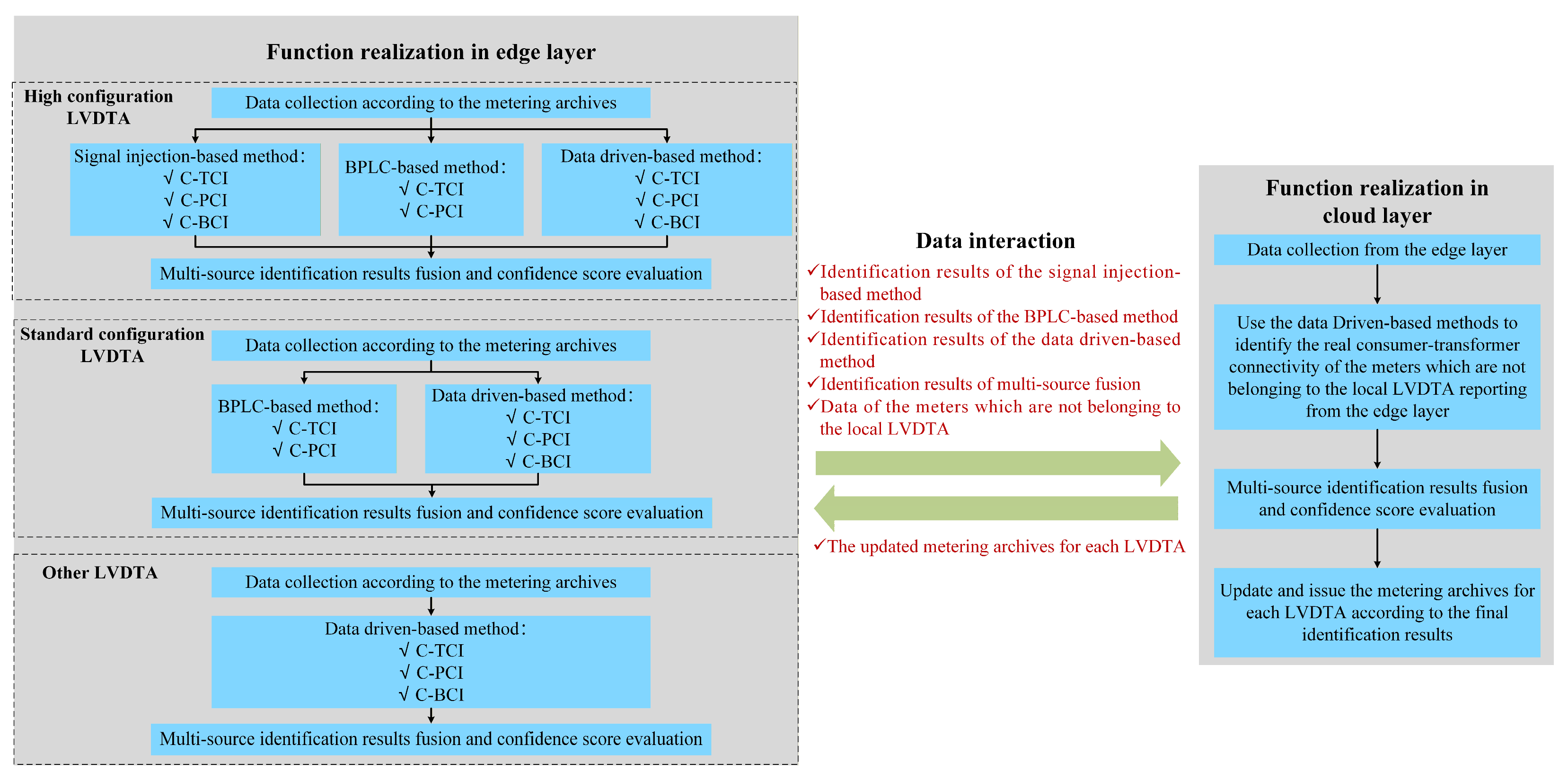
Based on the aforementioned system architecture, this section further proposes the function realization and data interaction model for LVDN TI applications, as shown in Figure 13. “√” indicates that the type of TI carried out in Figure 13.

Figure 13. Diagram of function realization and data interaction of LVDN TI applications.

In terms of function realization, edge computing terminals are configured with different TI methods according to the application requirement of each method. TI on the edge side is only for meters that are in the metering archives of the target LVDTA, and the multi-source fusion identification results are reported to the cloud side. All the measurement data is collected on the cloud side, and the global re-attribution analysis can be conducted, thereby achieving the complete identification of the C-TC for each LVDTA. Further, the complete identification of the C-PC and C-BC can be realized. On this basis, the metering archives can be updated and issued back to each LVDTA, and the topology can be re-identified based on the updated metering archives. Through cloud–edge iterative optimization, the accurate and reliable identification of the LVDN topology can be achieved.

In terms of data interaction, the edge computing terminal primarily reports TI results and measurement data. The measurement data mainly includes the time-series data referring to 15 min interval monitoring data (energy, voltage, current, active power, power factor, etc.) from various monitoring nodes in the area (including LV buses, LV branches, and smart meters). As the volume of this data is immense, uploading the full set would impose significant pressure on the uplink communication and cloud platform storage. Therefore, the system considers reporting only the time-series data of meters identified by the edge as “non-native” (not belonging to the target LVDTA) and meters with key consumption characteristics in the target LVDTA. This provides data for the cloud to perform re-allocation calculations for non-native meters. The cloud then issues the updated metering archive, enabling the edge to re-identify it.

5.4. Computational Complexity Analysis

The computational complexity mainly lies in posterior responsibility inference based on the EM algorithm, which can be analyzed as follows:

$${\vartheta }_{\mathrm{E}\text{-}\mathrm{step}}=\vartheta (M\times N\times S\times \overline{T})$$

(36)

$${\vartheta }_{\mathrm{M}\text{-}\mathrm{step}}=\vartheta (S\times N^2\times M\times \overline{T})$$

(37)

$${\vartheta }_{\mathrm{EM}}=\vartheta (S\times N^2\times M\times \overline{T})$$

(38)

where $\overline{T}={\displaystyle \sum _{i,s}|}{𝒪}_i^{(s)}|/MS$ is the average number of non-outcome-missing time windows per meter per evidence source.

In practical deployments, edge computing terminals commonly adopt ARM-based SoCs (e.g., Cortex-A9-class processors) with a typical configuration of a 1.0 GHz CPU, 2 cores, and 1.0 GB RAM, which is sufficient for non-real-time analytics tasks in PIoT environments. In a typical LVDTA with M = 200, S = 3, T = 673, and N = 3, the computation of each EM iteration is approximately 3.7 × 10⁶ operations, and each EM iteration completes in approximately 300 ms with Python 3.13 coding. Calculated based on the maximum number of iterations, the total computation time is approximately 300 s. As topology identification is a quasi-static asset management task rather than a real-time protection/control function, EM can be executed at the edge for daily computation. Moreover, with the continuous advancement of embedded processor and accelerator technologies, the edge computing capability is expected to further improve, making EM-based training and confidence-aware TI increasingly practical for deployment on the edge side.

6. Conclusions

Aiming at the problems that the current LVDN TI research lacks the consideration of multiple method fusion and the confidence evaluation of identification results, and that the reliability and practicality of identification results are difficult to guarantee, this paper proposes a Ca-TI method for LVDNs based on the WSLM and CCCCG-DS evidence fusion, obtaining the following conclusions:

(1)

The proposed framework delivers reliable TI results under practical bad-data conditions. Compared with naive agreement-based fusion, the proposed method mitigates performance collapse caused by a single unreliable method and remains robust under increasing measurement noise and missing data.

(2)

Beyond accuracy, the proposed method can provide the meter-level confidence to support deployment: high-confidence meters can be trusted with minimal verification, while low-confidence meters can be prioritized for verification, enabling a practical “trust-and-verify” workflow that reduces unnecessary on-site checks.

(3)

We further analyzed the preset threshold sensitivity for the proposed method. The confidence thresholds exhibit stable behavior over a broad range, indicating that the proposed confidence scoring supports consistent high-confidence decision quality and error recall. The confidence weight coefficient remains stable in moderate-to-low ranges, whereas overly emphasizing the uncertainty term can weaken conflict-driven risk signaling; this provides clear guidance for practical parameter selection.

Future work will focus on the physical interpretability of TI confidence computation and relaxing the implicit independence assumption in D-S fusion because different TI methods may share common physical features (e.g., voltage/power variations), leading to correlated evidence and potentially overconfident decisions. We will investigate dependence-aware evidence fusion by explicitly modeling inter-source correlation or applying correlation-aware discounting to improve confidence calibration. In addition, to support scalable and online maintenance under evolving operating conditions, we will explore reinforcement-learning-driven sparse update strategies that selectively trigger re-identification or field verification only for persistently low-confidence/high-conflict meters [38]. Finally, we will study how confidence-aware TI can better support downstream grid operations under high EV integration, following recent system-level assessments of EV impacts on distribution networks [39].

References

- Kalinga, T.; Banfield, B.; Knott, J.C.; Robinson, D.A. K-Means Clustering and Linear Regression for User Phase Identification, Verification, and Topology Determination Under Varied Smart Meter Penetration. Energies 2026, 19, 183. [Google Scholar] [CrossRef] [Scilit]
- Lei, Y.; Yang, F.; Feng, Y.; Hu, W.; Cheng, Y. A Two-Stage Topology Identification Strategy for Low-Voltage Distribution Grids Based on Contrastive Learning. Energies 2025, 18, 5886. [Google Scholar] [CrossRef] [Scilit]
- Zhang, Y.; Liu, S.; Jiang, J.; Yi, Y.; Li, Q. Research Review on Low-Voltage Intelligent Distribution Network Technology. Guangdong Electr. Power 2019, 32, 1–12. [Google Scholar]
- Wang, P.; Zhang, D.; Gan, L.; Zhang, Y. Key Technologies and Applications of Collaboration between Digital Power Grid and Internet of Things. Digit. Twins Appl. 2024, 1, 26–37. [Google Scholar] [CrossRef] [Scilit]
- Ge, H.; Xu, B.; Chen, W.; Zhang, X.; Bi, Y. Topology identification of low voltage distribution network based on current injection method. Arch. Electr. Eng. 2021, 70, 297–306. [Google Scholar]
- Fernandez, J.H.; Omri, A.; Di Pietro, R. Power grid surveillance: Topology change detection system using power line communications. Int. J. Electr. Power Energy Syst. 2023, 145, 108634. [Google Scholar] [CrossRef] [Scilit]
- Lai, X.; Cao, M.; Liu, S.; Sun, C. Low-Voltage Distribution Network Topology Identification Method Based on Characteristic Current. In Proceedings of the 2021 6th Asia Conference on Power and Electrical Engineering (ACPEE), Chongqing, China, 8–11 April 2021; pp. 1233–1238. [Google Scholar] [CrossRef] [Scilit]
- Zhou, C.; Dai, S.; Pan, Z.; Wu, H.; Chen, C. An Algorithm for Dynamic Identification of Low-Voltage Topology. J. Phys. Conf. Ser. 2023, 2428, 012036. [Google Scholar] [CrossRef] [Scilit]
- IEEE Std 1901–2020 (Revision of IEEE Std 1901–2010); IEEE Standard for Broadband over Power Line Networks: Medium Access Control and Physical Layer Specifications. IEEE: New York, NY, USA, 2021. [CrossRef] [Scilit]
- Lavenu, C.; Aldebert, T.; Caqueux, M.; Bretand, D.; Chapoulie, A. Phase Detection in PLC-Based Advanced Metering Infrastructures. In Proceedings of the 25th International Conference on Electricity Distribution (CIRED 2019), Madrid, Spain, 3–6 June 2019; p. 136. [Google Scholar]
- Xu, C.; Lei, Y.; Zou, Y. A Method of Low-Voltage Topology Identification. In Proceedings of the 2020 IEEE Conference on Telecommunications, Optics and Computer Science (TOCS), Shenyang, China, 11–13 December 2020; pp. 318–323. [Google Scholar] [CrossRef] [Scilit]
- Xu, M.; Li, R.; Li, F. Phase Identification with Incomplete Data. IEEE Trans. Smart Grid 2018, 9, 2777–2785. [Google Scholar] [CrossRef] [Scilit]
- Yi, Y.; Liu, S.; Zhang, Y.; Xue, Y.; Deng, W.; Li, Q. Phase Identification of Low-Voltage Distribution Network Based on Stepwise Regression Method. J. Mod. Power Syst. Clean Energy 2023, 11, 1224–1234. [Google Scholar] [CrossRef] [Scilit]
- Zhang, Y.; Yi, Y.; Deng, W.; Liu, S.; Zhou, L.; Lin, K.; Cai, Y. Consumer-Branch Connectivity Identification of Low-Voltage Distribution Networks Based on Data-Driven Approach. Prot. Control Mod. Power Syst. 2024, 9, 60–82. [Google Scholar] [CrossRef] [Scilit]
- Bariya, M.; Deka, D.; von Meier, A. Guaranteed Phase & Topology Identification in Three-Phase Distribution Grids. IEEE Trans. Smart Grid 2021, 12, 3605–3612. [Google Scholar] [CrossRef] [Scilit]
- Zhou, L.; Li, Q.; Zhang, Y.; Chen, J.; Yi, Y.; Liu, S. Consumer Phase Identification Under Incomplete Data Condition with Dimensional Calibration. Int. J. Electr. Power Energy Syst. 2021, 129, 106851. [Google Scholar] [CrossRef] [Scilit]
- Wang, Z.; Yu, T.; Huang, Y.; Wang, K.; Pan, Z. A New Topology Identification Method for Low-Voltage Distribution Network Based on U-Shaplets Feature Subsequence. Electr. Meas. Instrum. 2025, 62, 68–79. [Google Scholar]
- Zhou, L.; Zhang, Y.; Liu, S.; Li, K.; Li, C.; Yi, Y.; Tang, J. Consumer Phase Identification in Low-Voltage Distribution Network Considering Vacant Users. Int. J. Electr. Power Energy Syst. 2020, 121, 106079. [Google Scholar] [CrossRef] [Scilit]
- Tang, J.; Cai, Y.; Zhou, L.; Yi, Y.; Chen, G.; Liang, S.; Zhang, Y. Data-Driven Based Identification Method of Feeder-Consumer Connectivity in Low-Voltage Distribution Network. Autom. Electr. Power Syst. 2020, 44, 127–134. [Google Scholar]
- Li, H.; Liang, W.; Liang, Y.; Li, Z.; Wang, G. Topology Identification Method for Residential Areas in Low-Voltage Distribution Networks Based on Unsupervised Learning and Graph Theory. Electr. Power Syst. Res. 2023, 215, 108969. [Google Scholar] [CrossRef] [Scilit]
- Mauladdawilah, H.; Balfaqih, M.; Balfagih, Z.; Pegalajar, M.d.C.; Gago, E.J. Deep Feature Selection of Meteorological Variables for LSTM-Based PV Power Forecasting in High-Dimensional Time-Series Data. Algorithms 2025, 18, 496. [Google Scholar] [CrossRef] [Scilit]
- Elsafi, A.; Almohammedi, A.A.; Balfaqih, M.; Balfagih, Z.; Sabri, S. Comparative Analysis of Maximum Power Point Tracking Methods for Power Optimization in Grid Tied Photovoltaic Solar Systems. Discov. Appl. Sci. 2025, 7, 976. [Google Scholar] [CrossRef] [Scilit]
- Guo, X.; Xu, C.; Ming, Z.; Meng, B.; Yang, S.; Xu, L.; Zhu, Y. User-Feeder Topology Identification in Low-Voltage Residential Power Networks: A Clustering Fusion Approach. Energies 2025, 18, 4908. [Google Scholar] [CrossRef] [Scilit]
- Li, K.; Zhou, L.; Zhang, Y.; Liu, X.; Li, G.; Huang, G. Credibility Evaluation of Topology Identification Results in Low-Voltage Distribution Network Based on Quality of Measured Data. Autom. Electr. Power Syst. 2021, 45, 99–107. [Google Scholar]
- Zhang, H.; Zhao, J.; Wang, X.; Xuan, Y. Low-Voltage Distribution Grid Topology Identification With Latent Tree Model. IEEE Trans. Smart Grid 2022, 13, 2158–2169. [Google Scholar] [CrossRef] [Scilit]
- Zhou, Z.-H. A brief introduction to weakly supervised learning. Natl. Sci. Rev. 2018, 5, 44–53. [Google Scholar] [CrossRef] [Scilit]
- Khaleghi, B.; Khamis, A.; Karray, F.O.; Razavi, S.N. Multisensor data fusion: A review of the state-of-the-art. Inf. Fusion 2013, 14, 28–44. [Google Scholar] [CrossRef] [Scilit]
- Zadeh, L.A. Review of Shafer’s A Mathematical Theory of Evidence. AI Mag. 1984, 5, 81–83. [Google Scholar]
- Denœux, T.; Li, S. Frequency-Calibrated Belief Functions: Review and New Insights. Int. J. Approx. Reason. 2018, 92, 232–254. [Google Scholar] [CrossRef] [Scilit]
- Tang, Y.; Zhou, Y.; Ren, X.; Sun, Y.; Huang, Y.; Zhou, D. A New Basic Probability Assignment Generation and Combination Method for Conflict Data Fusion in the Evidence Theory. Sci. Rep. 2023, 13, 8443. [Google Scholar] [CrossRef] [Scilit]
- Fu, W.; Yu, S.; Wang, X. A Novel Method to Determine Basic Probability Assignment Based on Adaboost and Its Application in Classification. Entropy 2021, 23, 812. [Google Scholar] [CrossRef] [Scilit] [PubMed]
- Fei, L.; Li, T.; Ding, W. A State-of-the-Art Survey on Neural Computation-Enhanced Dempster-Shafer Theory for Safety Accidents: Applications, Challenges, and Future Directions. Neurocomputing 2025, 643, 130419. [Google Scholar] [CrossRef] [Scilit]
- Zhang, J.; Hsieh, C.-Y.; Yu, Y.; Zhang, C.; Ratner, A. A Survey on Programmatic Weak Supervision. arXiv 2022, arXiv:2202.05433. [Google Scholar] [CrossRef] [Scilit]
- Zhang, J.; Yu, Y.; Li, Y.; Wang, Y.; Yang, Y.; Yang, M.; Ratner, A. WRENCH: A Comprehensive Benchmark for Weak Supervision. In Proceedings of the Neural Information Processing Systems (NeurIPS) Datasets and Benchmarks, Online, 6–14 December 2021. [Google Scholar] [CrossRef] [Scilit]
- Huang, L.; Ruan, S.; Decazes, P.; Denœux, T. Deep Evidential Fusion with Uncertainty Quantification and Reliability Learning for Multimodal Medical Image Segmentation. Inf. Fusion 2025, 113, 102648. [Google Scholar] [CrossRef] [Scilit]
- Zhao, K.; Li, L.; Chen, Z.; Sun, R.; Yuan, G.; Li, J. A Survey: Optimization and Applications of Evidence Fusion Algorithm Based on Dempster-Shafer Theory. Appl. Soft Comput. 2022, 124, 109075. [Google Scholar] [CrossRef] [Scilit]
- Gao, Y.; Wang, C.; Xin, J.; Liu, A.; Chen, Y. Calculation of Three-Phase Power Flow in Medium and Low-Voltage Distribution Network with Multiple Distributed Generators Taking Into Account Ground Impedance (1): Model. Proc. CSEE 2016, 36, 2619–2627. [Google Scholar]
- Kaloev, M.; Krastev, G. Comprehensive Review of Benefits from the Use of Sparse Updates Techniques in Reinforcement Learning: Experimental Simulations in Complex Action Space Environments. In Proceedings of the 2023 4th International Conference on Communications, Information, Electronic and Energy Systems (CIEES 2023), Plovdiv, Bulgaria, 23–25 November 2023. [Google Scholar] [CrossRef] [Scilit]
- Amann, G.; Escobedo Bermúdez, V.R.; Boskov-Kovacs, E.; Gallego Amores, S.; Giannelos, S.; Iliceto, A.; Ilo, A.; Chavarro, J.R.; Samovich, N.; Schmitt, L.; et al. E-Mobility Deployment and Impact on Grids: Impact of EV and Charging Infrastructure on European T&D Grids: Innovation Needs; Report No. MJ-09-22-246-EN-N; Publications Office of the European Union: Luxembourg, 2022. [CrossRef]
Disclaimer/Publisher’s Note: The statements, opinions and data contained in all publications are solely those of the individual author(s) and contributor(s) and not of MDPI and/or the editor(s). MDPI and/or the editor(s) disclaim responsibility for any injury to people or property resulting from any ideas, methods, instructions or products referred to in the content. |
© 2026 by the authors. Licensee MDPI, Basel, Switzerland. This article is an open access article distributed under the terms and conditions of the Creative Commons Attribution (CC BY) license.