


Abstract
Residential photovoltaic (PV)–battery systems are increasingly deployed to reduce electricity costs under time-of-use and demand-charge tariffs, yet their economic value depends critically on how storage is operated over time. Effective control must simultaneously address short-term energy costs, peak-demand exposure, and long-term battery degradation, all under substantial uncertainty in load and PV generation. While optimization-based approaches can achieve strong performance with accurate forecasts, they are sensitive to forecast errors, whereas learning-based methods often neglect degradation effects or deplete the battery prematurely, leading to suboptimal peak-shaving behavior. This paper proposes a forecast-free, degradation-aware reinforcement learning (RL) framework for residential PV–battery energy management that jointly addresses demand-charge mitigation and battery aging. The proposed controller internalizes both calendar aging and rainflow-based cycling degradation within its objective and incorporates demand-aware reward shaping with time-varying penalties on on-peak grid imports. In addition, a complementary state-of-charge reserve mechanism discourages premature battery depletion and improves responsiveness to late on-peak demand surges, despite the absence of explicit load or PV forecasts. Physical feasibility is guaranteed through an execution-time safety layer that enforces all device and operational constraints by construction. The proposed framework is evaluated on high-resolution residential datasets and compared against optimization-based baselines, including a day-ahead scheduler with perfect foresight and a receding-horizon MPC controller using short-horizon forecasts. Overall, the results show that the proposed RL controller substantially reduces demand charges and total electricity costs relative to forecast-based MPC while maintaining degradation-aware operation, demonstrating the potential of forecast-free reinforcement learning as a practical control strategy for residential PV–battery systems under demand-charge tariffs.
1. Introduction
The rapid deployment of residential photovoltaic (PV) systems, driven by decarbonization targets and declining module costs, is fundamentally reshaping electricity consumption at the distribution level. As PV penetration increases, behind-the-meter battery energy storage systems (BESSs) are increasingly adopted to mitigate variability, increase self-consumption, and reduce electricity costs under time-of-use (TOU) and demand-charge tariffs [1,2]. In many regions, demand charges—based on short-interval maximum grid import during predefined peak windows—constitute a substantial fraction of residential electricity costs, making effective peak shaving a primary operational objective. However, the economic value of residential storage critically depends on how the battery is operated over time under uncertainty in household load and PV generation, rather than merely on its installed capacity [3,4].
Battery operation involves an inherent multi-objective trade-off. Aggressive charge–discharge strategies can reduce short-term electricity costs and suppress peak imports, but they accelerate battery degradation through both calendar aging and cycling mechanisms. Experimental and review studies show that lithium-ion batteries experience capacity fade and impedance growth as a function of state of charge (SoC), depth of discharge, temperature, and cycling intensity [5,6,7]. Consequently, dispatch strategies that neglect degradation effects often overestimate economic benefits and may result in premature asset wear. These observations motivate degradation-aware energy management strategies that explicitly balance operating cost against long-term battery health, particularly in residential settings where storage is cycled daily over extended lifetimes.
Optimization-based energy management systems remain the dominant paradigm for PV–battery scheduling. Mixed-integer linear programming (MILP) is commonly used for day-ahead planning, while model predictive control (MPC) enables receding-horizon operation with feedback [8,9]. These approaches naturally encode tariff structures, including demand charges through epigraph formulations, and provide transparent, auditable solutions. When accurate forecasts of load and PV generation are available, optimization-based controllers can achieve near-optimal schedules. However, their performance degrades under forecast errors, which are unavoidable in residential environments due to weather variability and stochastic user behavior. Robust and stochastic extensions partially address this limitation but introduce conservatism, modeling complexity, and increased computational burden [10,11]. Moreover, incorporating realistic battery aging—particularly rainflow-based cycle degradation—further complicates optimization formulations and limits scalability [12,13].
Reinforcement learning (RL) has emerged as a promising alternative, offering a model-free paradigm that learns control policies directly from interaction with the environment. By avoiding explicit forecasting models, RL is inherently attractive for residential energy management under uncertainty [14,15]. Recent studies demonstrate that deep RL can achieve competitive economic performance under complex tariffs. However, several limitations remain in existing residential RL-based EMS studies. In particular, many RL-based controllers optimize short-term electricity cost without explicitly accounting for battery degradation, which can lead to overly aggressive cycling and premature capacity loss [15,16]. Moreover, practical deployment considerations—including constraint satisfaction, robustness across heterogeneous households, and reproducible performance under realistic operating variability—are not uniformly addressed across residential PV–battery RL studies.
Despite these advances, an important gap remains in the literature. Most RL-based energy management strategies do not explicitly address demand-charge operation, where peak imports occurring late within the on-peak window can dominate the electricity bill. In parallel, battery degradation is often omitted or represented through surrogate penalties without quantitative validation against physics-based aging metrics used for evaluation and monetization. Several optimization-based studies incorporate more detailed degradation formulations; however, these approaches typically rely on explicit load and PV forecasts and introduce substantial modeling and computational complexity. Consequently, learning a forecast-free control policy that jointly anticipates peak-demand timing under demand charges while managing battery degradation consistently with physics-based evaluation represents an important and largely unexplored direction for residential PV–battery EMS research.
This paper addresses these challenges by proposing a forecast-free, degradation-aware reinforcement learning framework for residential PV–battery energy management under demand-charge tariffs. The proposed controller internalizes degradation-aware surrogate cost terms aligned with both calendar aging and cycle aging mechanisms during training, while full rainflow-based degradation assessment is used for ex-post performance evaluation. This design balances computational tractability during learning with physically grounded degradation modeling during benchmarking. To address demand charges, we introduce demand-aware shaping mechanisms with time-varying penalties during on-peak periods, encouraging strategic retention of stored energy and robust mitigation of late peak imports. In addition, a dynamically enforced state-of-charge reserve during on-peak operation discourages premature battery depletion and improves robustness to late demand surges. Physical feasibility is ensured through an execution-time safety layer that enforces inverter power limits and SoC bounds, enabling safe deployment independently of the learning process.
Although policy training requires offline interaction over representative seasonal data, the learned controller is executed during deployment as a lightweight feedforward mapping. As a result, real-time operation requires only a forward pass of the neural network, leading to very low inference latency compared with optimization-based controllers that must repeatedly solve constrained optimization problems at each control step. The proposed framework is evaluated on high-resolution public residential datasets using seasonal out-of-sample testing and stress scenarios. Performance is compared against two optimization-based baselines: a day-ahead scheduler with perfect foresight and a receding-horizon MPC controller using short-horizon forecasts. This evaluation setup enables a systematic comparison between forecast-free learning and optimization-based control under identical tariffs, device constraints, and degradation models.
The contributions of this work are threefold. First, we develop a forecast-free reinforcement learning framework for residential PV–battery energy management under demand-charge tariffs. The proposed formulation incorporates battery degradation awareness during policy learning through surrogate cost terms that remain compatible with reinforcement learning training dynamics. This design enables degradation-aware control while avoiding reliance on explicit load or PV forecasts. Second, we introduce demand-aware reward shaping and adaptive state-of-charge reserve mechanisms that enable the controller to anticipate peak-demand timing within on-peak tariff windows. These mechanisms encourage strategic retention of stored energy during early on-peak periods and improve robustness to late peak-demand realizations. This design directly addresses a key operational challenge of demand-charge tariffs that is not explicitly treated in existing RL-based residential EMS studies. Third, we establish a transparent benchmarking framework for residential PV–battery control under demand-charge tariffs by evaluating forecast-free reinforcement learning against both a day-ahead optimizer with perfect foresight and a receding-horizon MPC controller under identical tariff definitions, device constraints, and degradation models. This evaluation isolates the impact of forecast dependence and provides a consistent basis for comparing learning-based and optimization-based control strategies across heterogeneous residential operating conditions.
The remainder of this paper is organized as follows. Section 2 reviews related work on PV–battery energy management systems. Section 3 formulates the problem, including the system model, tariff structure, and degradation representation. Section 4 presents the proposed reinforcement learning control framework. Section 5 describes the experimental setup, and Section 6 reports the experimental results. Finally, Section 7 concludes the paper.
2. Related Work
Research on PV–battery energy management spans three closely related directions: (i) optimization-based scheduling and receding-horizon control, (ii) learning-based control emphasizing operational safety, and (iii) battery aging models and their integration into control objectives. Forecasting assumptions and practical deployment considerations cut across these lines where they materially affect performance and feasibility.
2.1. Optimization-Based Energy Management
Optimization-based energy management systems (EMSs) remain the dominant baseline for PV–battery scheduling. In day-ahead operation, mixed-integer linear programming (MILP) formulations co-optimize grid exchange and battery set-points subject to state-of-charge (SoC) dynamics, power limits, tariff rules, and optional constraints such as export bans or demand charges. These approaches yield transparent schedules that are easy to audit and have been demonstrated in field-relevant settings [8].
Receding-horizon model predictive control (MPC) improves robustness by repeatedly solving a finite-horizon optimization problem using updated measurements and forecasts, thereby providing feedback while preserving explicit constraint handling [9]. Demand charges are typically handled via epigraph variables that penalize the maximum on-peak import within a billing window, and most formulations remain convex or near-convex when binary decisions are minimized.
Despite their strengths, optimization-based EMS depend critically on forecast quality. Forecast errors in load, PV generation, or electricity prices can misalign charge–discharge decisions and reduce economic performance, particularly under tariffs with strong temporal structure such as time-of-use periods and demand charges. Robust and stochastic variants mitigate this sensitivity by optimizing against uncertainty sets or scenarios, trading conservatism for expected performance [10,11]. However, these approaches increase modeling and computational complexity and still rely on explicit forecast representations.
Incorporating battery degradation further complicates optimization-based EMS. Throughput-based or piecewise-linear aging proxies preserve tractability and already alter optimal schedules compared with cost-only formulations [12]. More detailed treatments embed rainflow-based cycle counting within MILP or MPC frameworks to reflect depth-dependent cycling damage [13]. While effective, such formulations remain forecast-dependent and can be sensitive to modeling assumptions, motivating complementary approaches that learn directly from interaction.
2.2. Reinforcement Learning for Energy Management
Reinforcement learning (RL) provides a model-free alternative that learns control policies directly from interaction with the environment, avoiding explicit forecasts of load or PV generation. Surveys highlight its ability to handle nonlinear dynamics, nonconvex tariffs, and nonstationary conditions in energy systems [14,17]. Early applications to microgrids and residential EMS demonstrate that deep RL policies can match or exceed heuristic or rule-based baselines under stochastic conditions [15].
Policy design choices are critical for performance and deployability. Continuous-action policies exploit inverter limits more effectively than discrete control, while informative state representations—including time features and recent measurements—help reduce myopic decisions. Reward design plays a central role: cost-only objectives can encourage aggressive cycling, whereas incorporating degradation-related terms moderates battery usage.
A major challenge is operational safety. Unconstrained RL may explore infeasible actions during training and violate SoC or power limits at deployment. Safe RL approaches typically cast control as a constrained Markov decision process (CMDP) and enforce constraints using primal–dual methods or trust-region algorithms such as Constrained Policy Optimization (CPO) [18,19]. In power systems, CMDP-based deep RL has demonstrated improved adherence to operational limits while maintaining competitive economics [20]. However, these methods introduce additional training complexity, sensitivity to constraint tuning, and nontrivial convergence issues [17,21].
An alternative line of work enforces feasibility through execution-time safety layers or action projection, ensuring that only admissible actions are applied to the physical system. This approach avoids explicit constraint optimization while guaranteeing physical feasibility, but has been less explored in conjunction with degradation-aware objectives and demand-charge-driven peak management.
2.3. Battery Aging Models and Their Integration
Lithium-ion battery aging arises from both calendar mechanisms during storage and cycling mechanisms driven by charge–discharge usage. Aging rates depend on state of charge, depth of discharge, temperature, and current rate, as documented in extensive experimental studies [5,6,7]. For energy management, semi-empirical models are commonly adopted to balance fidelity and tractability. Calendar aging is typically modeled as a function of SoC and temperature, while cycling aging is represented through depth-dependent damage functions.
Rainflow counting, standardized in ASTM E1049–85, provides a principled way to map irregular SoC trajectories to equivalent charge–discharge cycles [22,23]. These cycles can be converted to equivalent full cycles or monetized life loss, enabling direct comparison of operational strategies. For lithium iron phosphate (LFP) cells, temperature-dependent models offer practical coefficients suitable for system-level studies [24].
In optimization-based EMS, aging has been integrated either through throughput proxies or rainflow-derived costs, significantly affecting dispatch decisions [12,13]. In learning-based control, aging is typically internalized via reward shaping or life-consumption penalties, although many studies still omit explicit aging models, limiting the credibility of long-term economic comparisons.
2.4. Positioning of This Work
In contrast to prior studies, this work combines a degradation-aware objective with forecast-free reinforcement learning and explicit physical feasibility enforced at execution time. The controller internalizes both calendar and cycle aging while learning to manage peak imports under demand-charge tariffs without relying on load or PV forecasts. Performance is benchmarked against optimization-based baselines under identical tariffs, constraints, and aging models, enabling a transparent assessment of trade-offs between forecast-driven and learning-based control.
3. Problem Formulation
We consider the operation of a residential photovoltaic (PV) system coupled with a battery energy storage system (BESS) over a finite time horizon discretized into T intervals of duration . At each time step , household load and PV generation are realized, and the controller selects a battery power command , where denotes battery discharge and denotes battery charging.
3.1. Battery Dynamics and Power Balance
The battery state of charge (SoC), denoted , evolves according to
where , E is the nominal battery energy capacity, and and are the charging and discharging efficiencies.
The instantaneous grid power import is given by
with any excess generation exported to the grid.
Battery operation is subject to physical constraints
where and define the allowable SoC window and is the maximum charge/discharge power.
3.2. Energy Cost and Demand Charge
Electricity imported from the grid is billed under a time-varying tariff , yielding the cumulative energy cost
In addition, a demand charge is applied based on the maximum grid import during designated on-peak periods :
where is the demand charge rate.
3.3. Battery Aging and Degradation Modeling
Battery degradation is explicitly modeled to quantify lifetime wear induced by both time-dependent (calendar) aging and usage-dependent (cycling) aging. The aging model is used for performance evaluation and cost monetization and is implemented consistently across all control methods.
3.3.1. End-of-Life Definition
Battery end of life (EoL) is defined at an energy-based state-of-health threshold by default. All degradation metrics are expressed as fractional life consumption relative to this limit.
3.3.2. Calendar Aging
Calendar aging captures capacity loss due to storage at a given state of charge and temperature. We adopt a separable, multiplicative rate model calibrated for LFP cells:
where R is the universal gas constant, is the ambient (or cabinet) temperature in °C, and is a convex SoC-dependent multiplier normalized at a reference SoC . Following Vetter et al. [5], Birkl et al. [6], Schimpe et al. [24], we parameterize
All calendar-aging coefficients are fixed from LFP literature values (Section 5).
3.3.3. Cycling Aging
Cycling-induced degradation is evaluated from the SoC trajectory using rainflow cycle counting (ASTM E1049–85), which yields cycle depths and mean SoC levels [22]. Life consumption is computed via Miner’s rule with a Wöhler-type life curve:
where captures the mild dependence on mean SoC. Cycling parameters are selected from LFP cycle-life studies consistent with Peterson et al. [23], Schimpe et al. [24]. For reporting purposes, the equivalent full cycles (EFC) metric is
3.3.4. Total Degradation and Monetization
Total life consumption over the horizon is
Degradation is monetized as
where is derived from the installed battery cost and the chosen EoL threshold.
3.3.5. Rainflow-Based Degradation Evaluation
Rainflow counting is applied offline to the realized SoC trajectory for evaluation and comparison across controllers. During RL training, a calibrated throughput-based proxy consistent with (11) is used for computational efficiency. All reported degradation results are computed using the exact rainflow-based formulation.
3.4. Unified Control Objective
Combining energy cost, demand charge, and battery degradation, the residential PV–battery energy management problem is formulated as
is considered under different information assumptions.
4. Methods
The unified optimization problem in (15) is evaluated under different information patterns, corresponding to distinct control paradigms. All controllers share the same system model, constraints, tariff structure, and degradation formulation, and differ only in the information available at decision time. Three approaches are considered: a day-ahead optimization benchmark (DA), a receding-horizon Model Predictive Control (MPC) strategy, and a reinforcement learning (RL)–based controller. This section presents the control strategies evaluated in this work and focuses exclusively on how each control method exploits available information and how it is implemented in practice. The DA and MPC strategies serve as optimization-based baselines, highlighting the impact of information availability and receding-horizon operation. The RL approach is designed to learn an implicit control policy capable of handling uncertainty and nonlinear trade-offs without explicit reliance on forecasts.
4.1. Day-Ahead Optimization (DA) Method
The day-ahead (DA) strategy represents an idealized optimization benchmark in which full knowledge of all exogenous signals over the entire scheduling horizon is assumed. Residential load, photovoltaic generation, electricity prices, and ambient temperature profiles are treated as perfectly known for the full day. Specifically, the controller has access to the realized sequences
and solves (15) once to produce an open-loop schedule for the entire horizon. Demand charges are handled exactly, as the maximum on-peak grid import over the full horizon is known at optimization time.
This setting provides an idealized lower bound on achievable operating cost and is used strictly as a performance reference. Day-ahead scheduling with explicit tariff components is widely used as a baseline in residential energy management studies [25]. While unattainable in practice, this benchmark is useful for quantifying the performance gap induced by uncertainty and limited information in online control schemes.
4.2. Receding-Horizon Model Predictive Control (MPC)
The MPC controller operates in a receding-horizon manner. At each time step t, it solves a finite-horizon instance of (15) over a prediction horizon H using forecasts of the exogenous signals,
where and denote the load and PV generation forecasts issued at time t.
At each time step t, MPC applies the control action before repeating the optimization at . We write the generic MPC step as
where denotes the measured state (including SoC and tariff indicators), and is the same cost functional as in (15) but evaluated using the forecasts over the horizon H. This receding-horizon structure is a standard and effective approach for residential PV–battery energy management under uncertainty [26].
Demand charges are incorporated through an augmented state variable representing the maximum on-peak grid import observed so far. During on-peak periods, this state evolves according to
allowing MPC to account for incremental demand-charge penalties without requiring full knowledge of future peak realizations.
In our implementation, short-term forecasts of residential load and photovoltaic generation are obtained using a simple persistence approach, i.e., near-future values are assumed equal to the most recently observed measurements. Persistence forecasting is commonly adopted as a transparent and strong baseline for short-term horizons in residential energy forecasting studies [27]. Under this setting, MPC can partially compensate for forecast errors through online re-optimization in a receding-horizon fashion. However, its performance remains sensitive to both the prediction horizon length and forecast accuracy, particularly for demand-charge mitigation when unexpected late on-peak load spikes occur. Consequently, MPC serves as a strong and interpretable baseline that explicitly enforces physical and operational constraints while operating in closed loop. At the same time, its inherent limitations under uncertainty motivate the learning-based control strategy introduced next.
4.3. Reinforcement Learning Control
The reinforcement learning (RL) controller operates in a fully closed-loop manner without relying on explicit forecasts of residential load or photovoltaic (PV) generation. Instead, the control policy is learned directly from interaction with the environment using instantaneous measurements of the system state, including battery state-of-charge (SoC), net load conditions, time-of-day features, and tariff indicators. This design enables the controller to respond adaptively to uncertainty while avoiding the brittleness associated with forecast errors.
4.3.1. RL Paradigm and Algorithmic Rationale
We adopt a continuous-control actor–critic framework, which is well suited to residential PV–battery energy management problems characterized by continuous action spaces, nonlinear system dynamics, and nonconvex cost structures induced by time-varying tariffs and demand charges. Actor–critic methods have demonstrated strong empirical performance and scalability in energy system applications, particularly when long-term economic objectives must be balanced against short-term operational considerations [28,29]. In addition, off-policy actor–critic formulations enable efficient reuse of historical experience, which is essential for learning over long horizons and for capturing delayed economic effects associated with demand charges. This property is particularly important in residential settings, where demand-charge impacts may only manifest at the end of a billing period.
Let denote the parameterized policy mapping the observed state to a charging or discharging action . The policy parameters are optimized to minimize the expected cumulative cost over an episode,
where corresponds to the same operational objective defined in Section 3, including energy costs, demand charges, and battery degradation.
4.3.2. Safety-Aware Action Execution
To guarantee physical feasibility, all actions proposed by the policy are passed through an execution-time safety layer that enforces battery power and SoC constraints. Denoting the raw policy output by , the applied control is
where denotes projection onto the admissible action set defined by device limits and SoC bounds. This ensures constraint satisfaction by construction, independently of the learning process. Such safety-layer architectures are increasingly adopted in energy and power system control to combine learning-based policies with strict operational guarantees [20]. Importantly, the projected control input defined above is directly used in the state-transition dynamics governing the battery state of charge (SoC). In particular, the SoC update equation is evaluated using the projected action rather than the raw policy output, and the resulting SoC is maintained within the admissible bounds at every time step. Consequently, battery power limits and SoC constraints are enforced throughout the closed-loop operation, and infeasible actions never propagate into the system dynamics. Constraint satisfaction therefore holds over the entire episode trajectory by construction, without relying on penalty terms or post hoc corrections.
4.3.3. Demand-Aware Reward Shaping
Demand charges introduce a non-additive cost component that depends on the maximum grid import during on-peak periods. To expose this structure to the learning agent, an auxiliary peak-tracking state is maintained, evolving as
where denotes the grid import power.
The corresponding demand-charge increment is reflected through a shaping term proportional to the marginal increase in peak demand. To emphasize late on-peak violations, the penalty is scaled by a time-varying weight,
where controls the amplification near the end of the on-peak window and determines the steepness of the ramp. This structure biases the policy toward mitigating late on-peak demand spikes, which are particularly costly under demand-charge tariffs.
4.3.4. Time-Varying SoC Reserve Shaping
While demand-aware shaping penalizes peak grid imports, it does not by itself prevent premature battery depletion early in the on-peak period. To address this failure mode, a complementary reserve-shaping term is introduced that biases the policy toward preserving stored energy for late on-peak uncertainty.
This mechanism is implemented as a soft, time-varying state-of-charge (SoC) floor penalty. A desired reserve trajectory is defined over the on-peak interval as
where and denote the reserve levels at the beginning and end of the on-peak window, respectively, and controls how aggressively the reserve requirement tightens over time.
The associated shaping cost is then given by
where is the actual battery SoC. This penalty is soft and state-dependent, allowing the policy to violate the reserve when economically justified, while discouraging systematic early depletion.
4.3.5. Calendar-Aging–Aware SoC Dwell Shaping
While the degradation term in the base cost captures both calendar and cycling aging contributions, directly optimizing such long-horizon effects through sparse terminal penalties can be challenging for policy-gradient methods. In particular, calendar aging depends not only on instantaneous SoC levels but also on the duration for which the battery dwells at elevated SoC, a temporal dependency that is weakly observable through short-term rewards. To explicitly expose this mechanism during learning, we introduce an SoC dwell–aware shaping term that biases the policy away from prolonged operation at high SoC.
This effect is modeled through a soft dwell penalty that activates when the battery SoC exceeds a predefined threshold . The corresponding shaping cost is defined as
where denotes the instantaneous battery SoC and controls the strength of the penalty. By penalizing sustained residence at high SoC rather than individual charging actions, this term directly targets the dominant drivers of calendar aging identified in physics-based battery models.
To further regularize long-term SoC behavior, an additional anchoring term is introduced that softly attracts the SoC toward a nominal operating point , chosen near mid-range SoC where calendar aging rates are minimized. This anchor penalty is expressed as
with determining the degree of attraction. Unlike hard constraints, this quadratic term preserves policy flexibility, allowing deviations from the anchor when required by economic or demand-charge considerations.
Together, the dwell and anchor penalties act as a temporal regularizer that shapes the SoC trajectory toward calendar-aging–benign regions of the state space, without explicitly constraining feasible operation. Importantly, these terms are applied during training only and serve to guide the policy toward degradation-aware behavior that generalizes across operating conditions. This design complements the physics-based degradation cost model by providing dense, interpretable learning signals aligned with the underlying aging mechanisms.
4.3.6. Unified Reward Signal
The total per-step reward combines the instantaneous energy cost, the incremental demand-charge contribution, battery degradation proxies, and the shaping terms described above. Importantly, both demand-aware and reserve shaping terms are aligned with the original economic objective and do not introduce additional constraints or rule-based logic.
5. Experimental Setup
This section describes the datasets, preprocessing pipeline, tariff model, device parameters, degradation modeling, forecast signals, controller configurations, train–test protocol, and evaluation metrics used in all experiments. Particular emphasis is placed on battery degradation, which is treated as a co-equal performance dimension alongside operating cost and peak-import reduction.
5.1. Datasets and Preprocessing
We use circuit-aggregated residential electricity traces from the Pecan Street Dataport program [30]. From the Austin cohort we select twelve homes with strong rooftop PV and near-year coverage: dataid_661, 1642, 2335, 2361, 3456, 3538, 4767, 7536, 7719, 7800, 8156, 9278. Signals are at min and are timezone-aligned to America/Chicago. For each home we construct: (i) whole-home demand (kW), (ii) PV generation (kW, nonnegative), and (iii) ambient temperature (°C). To ensure comparability across sites, we apply a light PV calibration so that the clear-sky index’s midday (10:00–15:00) median is close to one and clip sporadic negative PV readings.
5.1.1. Temperature Source
Ambient temperature is obtained from the Meteostat archive [31] for Austin, TX (30.27°, −97.74°, 150 m). We fetch hourly observations, convert to America/Chicago, and upsample to 15 min by linear interpolation; small gaps (≤1 h) are interpolated and larger gaps are dropped. This aligns with the min resolution used for control and aging.
5.1.2. Missing-Data Policy
All signals are aligned to min in America/Chicago. We linearly interpolate gaps up to two consecutive steps (≤30 min) for load, PV, and temperature; longer gaps are not filled. A day is retained if at least stamped intervals are present for both load and PV; otherwise it is discarded. Temperature is not used as a retention criterion but is interpolated as above when available. Table 1 summarizes the final Austin cohort.
Table 1.
Cohort summary and PV–load characteristics (Austin homes).
5.2. Tariff Model and Parameters
We evaluate two residential tariff configurations. The primary case is a time-of-use (TOU) import price with a weekday on-peak window from 16:00–21:00 (off-peak otherwise), reflecting widely adopted residential schedules (e.g., PG&E E–TOU–C) [32]. PV exports receive Austin Energy’s Value of Solar (VoS) credit at a flat rate [33]. A second configuration adds a monthly on-peak demand charge, consistent with designs used by SRP and APS [34,35,36]. Table 2 lists the parameters we use.
Table 2.
Tariff parameters used in experiments.
The demand-charge parameter in Table 2 corresponds to a tariff in which demand charges are normally billed over a monthly cycle based on the maximum on-peak demand observed during the billing period. In the present study, controllers are evaluated on single-day windows. Accordingly, for experimental comparability, the demand charge is computed as the demand-charge rate multiplied by the maximum on-peak grid import within each evaluated day. This day-level proxy preserves the utility billing rule while enabling consistent day-by-day controller comparisons without aggregating over a full billing period.
- Implementation notes. (i) The on-peak indicator
 is true on weekdays between 16:00–21:00 local time. (ii) The demand charge is modeled via an epigraph variable y with constraints for and cost , ensuring consistency with the maximum on-peak demand definition. (iii) All prices are in USD; positive denotes import from the grid; exports are credited at .
5.3. Device Parameters
Table 3 lists the default battery and inverter parameters.
Table 3.
Device parameters (defaults).
5.4. Aging–Model Parameters (LFP/Graphite Cells)
We instantiate the calendar and cycling wear models from Section 3.3 for lithium iron phosphate (LFP)/graphite cells using literature–consistent parameters. Calendar loss follows an Arrhenius form with a quadratic state-of-charge (SoC) modifier; cycling loss uses a Wöhler–type curve for depth-of-discharge with mild mean–SoC and temperature factors. Parameters are summarized in Table 4 and Table 5. Values are representative for stationary LFP cells and are consistent with empirical ranges reported in [6,23,24,37,38].
Table 4.
Calendar–aging parameters for LFP/graphite cells.
Table 5.
Cycling–aging parameters for LFP/graphite cells.
5.5. Aging Model and Monetization
We adopt the calendar and cycling formulations from Section 3.3 (Equations (6)–(12)) and fix all numerical coefficients to the LFP set reported in Section 5.4 (Table 4 and Table 5). Ambient temperature (Dataport, 15 min) is the temperature signal used in both models.
Over any horizon, the fraction-of-life consumption is given by
expressed relative to the capacity end-of-life threshold .
Battery wear is monetized as
where . For diagnostics, we also report equivalent full cycles (EFC) derived from the rainflow counts.
All controllers are evaluated under identical aging models and monetization parameters, ensuring that any observed differences in degradation arise solely from control decisions rather than modeling assumptions.
5.6. Forecast Signals
To ensure that differences in control performance are not driven by sophisticated prediction models, we adopt simple and transparent forecasting schemes that are widely used as baselines in residential energy management. Let denote the forecast horizon.
5.6.1. Load Forecast
Residential demand over the horizon is predicted using a persistence-based model that blends the most recent observation and the corresponding time-of-day value from the previous week,
with , which provides a simple yet effective short-term baseline.
5.6.2. Photovoltaic Forecast
PV generation is forecast using a clear-sky persistence model. A normalized clear-sky profile is computed for the Austin site using pvlib (Ineichen model) Python library (version 0.13.1) [39] and scaled to each home to obtain a site-specific envelope . The PV forecast is then given by
which extrapolates the current clear-sky index forward in time. This approach captures diurnal structure while remaining robust and computationally light.
5.6.3. Temperature Forecast
Ambient temperature over the horizon is predicted using persistence,
which is sufficient for short-term aging and efficiency calculations at the 15 min resolution considered.
5.7. Controllers and Hyperparameters
We evaluate three controller classes under the unified economic objective defined in Section 3. All controllers share the same system model, tariff structure, device limits, and degradation formulation, and differ only in how future information is handled and how decisions are generated. In particular, DA_perfect uses perfect foresight solely as a non-implementable oracle lower bound, MPC relies on the simple baseline forecasts defined in Section 5.6 (not advanced predictors), and RL_SAC executes without any explicit PV/load forecasting.
5.7.1. Day-Ahead Optimization (DA)
The day-ahead benchmark solves a single optimization problem over a full 24 h horizon using perfect foresight of all exogenous signals, including residential load, PV generation, prices, and temperature. Specifically, the realized trajectories are assumed known at decision time. The unified problem is solved once per day, producing an open-loop schedule that exactly internalizes energy costs, demand charges, and battery aging. A terminal SoC band is enforced. This oracle controller is not implementable in practice and serves solely as a lower bound on achievable cost.
5.7.2. Model Predictive Control (MPC_H56)
The MPC controller operates in closed loop using a receding-horizon strategy. At each time step, a finite-horizon instance of the unified optimization problem is solved over a prediction horizon of time steps (14 h) using the short-term forecasts described in Section 5.6. Only the first control action is applied before the horizon is shifted forward and the optimization is repeated.
The horizon length is chosen to reflect a realistic short-term MPC setting. A 14 h horizon is sufficient to capture the structure of on-peak demand periods and the intraday evolution of photovoltaic generation, which are the dominant drivers of demand charges in this application. Accordingly, represents a principled compromise that preserves forecast realism while enabling anticipative control.
A terminal state-of-charge (SoC) band identical to the day-ahead (DA) controller is enforced at the end of each prediction horizon. Demand charges are handled by tracking the running maximum of on-peak grid import within the billing period, which is updated online.
5.7.3. Reinforcement Learning (RL_SAC)
The RL_SAC controller is trained to directly minimize the same economic objective through interaction with the environment, without relying on explicit forecasts or solving an optimization problem online. The policy observes the current system state, including battery SoC, instantaneous load and PV generation, calendar indicators, and on-peak flags, and outputs a continuous real-power setpoint subject to device limits. Operational requirements, including demand charge mitigation and late-peak reserve preservation, are enforced through explicit reward shaping rather than hard constraints. In particular, time-varying penalties are applied to grid imports during on-peak periods and to low SoC levels near the end of the peak window, encouraging anticipatory reserve management. The RL agent is trained exclusively on the training months and evaluated out-of-sample on the test period. Table 6 lists default hyperparameters.
Table 6.
RL hyperparameters (defaults; identical across homes).
5.8. Train–Test Protocol
All experiments follow a fixed and identical train–test protocol to ensure a fair comparison across controllers. The available data for each home are split seasonally into a training period spanning March–August and a test period spanning September–February. This split exposes controllers to diverse operating conditions while preventing information leakage across seasons.
The reinforcement learning (RL) controller is trained exclusively on data from the training period. Model parameters are fixed after training and the learned policy is evaluated out-of-sample on the test period. No test data are used during training or hyperparameter selection. Day-ahead (DA) and MPC controllers do not require training and are evaluated directly on the test period using the same system parameters and tariff settings.
5.9. Performance Metrics and Error/Uncertainty Analysis
We report complementary metrics capturing economic performance, peak-import exposure, and battery-health outcomes. Economic performance is quantified by total electricity cost and its decomposition into energy and demand-charge components. Peak management is assessed using the maximum on-peak grid import and related peak statistics. Battery health is evaluated using (i) monetized degradation cost , (ii) its calendar and cycling components and under the adopted aging model, and (iii) physical stress proxies including energy throughput and equivalent full cycles (EFCs).
Because time-series observations within a home are temporally correlated, uncertainty is not computed over time steps or days. Instead, for each controller and each metric, we first compute a per-home aggregate over the evaluation horizon (e.g., mean daily cost, mean daily on-peak maximum import, cumulative degradation). We then summarize the distribution of these per-home aggregates across the cohort of N test homes and report confidence intervals (CIs) accordingly. Thus, all CIs shown in tables and figures reflect variability across homes under the fixed evaluation protocol described above.
In this control-oriented setting, performance error is therefore not defined relative to a prediction target, but rather through dispersion and deviation in achieved operational outcomes. Specifically, control error is captured by cross-home variability in per-home performance metrics (quantified via confidence intervals and distributional summaries), as well as by deviations relative to reference baselines such as the day-ahead perfect-information controller and the MPC benchmark.
In addition to reporting cohort-level confidence intervals, several results are presented using distributional visualizations (e.g., boxplots and per-home comparisons). These figures provide a complementary descriptive statistical view, revealing variability, skewness, and outliers across the residential cohort. This distributional perspective is particularly important in residential energy systems, where controller performance can vary substantially across households due to differences in load profiles, PV capacity, and usage patterns.
5.10. Implementation Details
All experiments were executed in a cloud-hosted Jupyter environment (Linux backend, Python 3.10). Day-ahead and MPC optimizations are formulated in cvxpy Python optimization modeling library (version 1.7.3) [40,41] and solved using the open-source HiGHS linear optimization solver [42]. The reinforcement learning controller is implemented in PyTorch (version 2.5.1) [43], with GPU acceleration used when available.
The reinforcement learning controller is trained episodically over daily horizons, with each episode corresponding to one full day of operation and initialized at a fixed state-of-charge. All reward-shaping coefficients, time-varying penalty ramps, and battery-reserve parameters are fixed a priori and shared across all homes and experimental scenarios. No per-day or per-home tuning is performed, ensuring that observed performance differences reflect control capability rather than hyperparameter adaptation.
Clear-sky PV envelopes are computed using pvlib [39]. Cycle aging diagnostics are obtained via ASTM E1049–85 rainflow counting [22]. All controllers are evaluated under identical numerical tolerances, time discretization, and tariff logic to ensure reproducibility and fair comparison.
6. Experimental Results
This section presents the empirical evaluation of the proposed PV–battery control framework on the Austin residential cohort (Table 1), using a 15 min resolution ( min) and the seasonal out-of-sample splits defined in Section 5. All controllers operate under identical tariff structures and demand-charge models (Table 2), device limits, and degradation monetization parameters specified in Section 5.2, Section 5.3 and Section 5.4.
We compare four strategies: a PV-only baseline without storage, a day-ahead optimization benchmark with perfect information (DA), a receding-horizon model predictive controller (MPC_H56), and a safe deep reinforcement learning (RL_SAC) controller that operates without explicit forecasts while enforcing state-of-charge, power, and terminal constraints by construction. Outcomes are computed per household and per day, and subsequently aggregated across homes, with uncertainty reported as mean ± 95% confidence intervals (CI).
We first establish a headline economic comparison across homes by decomposing the electricity bill into energy and demand-charge components, revealing the primary sources of cost differences among controllers. We then investigate peak-demand behavior in depth, using paired per-home analyses and distributional metrics to demonstrate systematic reductions in on-peak demand achieved by the proposed RL controller relative to MPC. Battery degradation is subsequently examined through an explicit separation of calendar and cycling contributions, supported by time-series evidence that links degradation outcomes to learned state-of-charge management. Selected operational case studies further illustrate how the RL policy allocates energy across the day to mitigate both early and late demand peaks. Finally, the proposed approach is positioned with respect to representative state-of-the-art residential energy-management methods through a structured comparative analysis that highlights key methodological and performance distinctions.
6.1. Experiment 1: Economic Performance Across Controllers
Experiment 1 provides a headline economic comparison across homes on the evaluation window. For each home and day, we report the total electricity bill , where is the energy charge and is the demand charge. Battery degradation cost is computed and logged but analyzed separately in the degradation-focused experiment.
6.1.1. Aggregate Cost Comparison
Table 7 reports the mean daily cost components across homes together with confidence intervals (CIs). Each mean is computed by first averaging over evaluation days for each home and then averaging across homes, so that each home contributes equally to the aggregate statistics. Confidence intervals therefore quantify cross-home uncertainty in economic performance rather than day-to-day variability within a single household.
Table 7.
Mean daily cost components across homes ( CI).
The PV-only baseline exhibits the highest total cost, with a mean of $40.54/day, dominated by demand charges ($36.24/day). This confirms that photovoltaic generation alone is insufficient to control peak demand under the considered tariff structure.
As expected, DA_perfect achieves the lowest total cost, with a mean total bill of $8.61/day and a demand charge of only $5.34/day. This represents a lower bound on achievable cost, enabled by perfect foresight of future load and PV generation.
Among implementable controllers, MPC_H56 reduces demand charges substantially relative to PV-only, achieving a mean demand cost of $20.46/day and a total cost of $24.09/day. The proposed RL_SAC controller further improves upon MPC, reducing the mean demand charge to $11.74/day and the total cost to $15.25/day. This corresponds to an average reduction of approximately $8.8/day in total cost and $8.7/day in demand charges relative to MPC_H56.
Energy costs remain of comparable magnitude across all battery-based controllers (approximately $3.3–$3.6/day), indicating that the observed differences in total cost are primarily driven by demand-charge mitigation rather than energy arbitrage.
6.1.2. Mean Cost Components and Uncertainty Analysis
Figure 1 visualizes the same results by decomposing the mean total cost into energy and demand components, together with confidence intervals across homes, providing an explicit uncertainty quantification of controller performance at the population level.
Figure 1.
Mean daily energy and demand cost components across homes, with CI.
While the table reports numerical values, the figure highlights two key aspects. First, demand charges dominate the total bill for all controllers, especially for the PV-only and MPC cases. Second, the width of the confidence intervals reveals the degree of cross-home variability. DA_perfect exhibits the narrowest intervals, reflecting stable performance across homes. MPC_H56 shows the largest variability, indicating sensitivity to household-specific load and PV profiles. RL_SAC not only lowers the mean demand cost relative to MPC, but also reduces variability, suggesting more consistent performance across heterogeneous homes.
6.1.3. Distribution of Total Costs Across Homes and Days
Mean values may obscure heterogeneity across homes and evaluation days. We therefore complement aggregate statistics with distributional analysis, which provides a descriptive statistical view of variability, skewness, and tail behavior.
Figure 2 therefore shows the distribution of total daily costs pooled over all evaluated homes and days. The PV-only baseline exhibits the widest distribution, with a median total cost of approximately $40/day and a pronounced upper tail extending beyond $100/day, indicating frequent high-cost realizations. DA_perfect concentrates costs tightly near the lower bound, with a median of roughly $3/day and limited variability.
Figure 2.
Distribution of total daily electricity costs across all evaluated homes and days.
Comparing implementable controllers, MPC_H56 exhibits a median total cost of approximately $16/day and a broad upper tail reaching close to $90/day. RL_SAC achieves a substantially lower median of about $7–8/day, representing a reduction of roughly $8–9/day relative to MPC, while also exhibiting a narrower interquartile range. Importantly, the upper tail under RL_SAC is visibly reduced, indicating fewer extreme high-cost days. These results confirm that the average improvement of RL over MPC is accompanied by improved robustness, not merely by isolated best-case days.
6.1.4. Per-Home Demand Cost Comparison
Figure 3 reports the mean daily demand cost for each home, averaged over evaluation days. For every home, battery-based controllers substantially reduce demand charges relative to the PV-only baseline. While DA_perfect consistently achieves the lowest demand cost, RL_SAC improves upon MPC_H56 for all homes. The magnitude of improvement varies across households, with particularly large gains observed for Homes 7719, 8156, and 4767, where RL reduces demand charges by approximately $5–10/day relative to MPC. This per-home comparison serves as a robustness check, confirming that the observed aggregate improvements reported in Table 7 are not driven by a small number of favorable realizations but persist consistently across the residential cohort.
Figure 3.
Mean daily demand cost per home for all controllers.
6.1.5. Sensitivity to Reward-Shaping Parameters
To evaluate the robustness of the proposed time-varying demand and reserve shaping mechanisms, we conducted a targeted training-time sensitivity analysis on the dominant shaping parameters of the RL_SAC controller. Specifically, for Home 661, we independently perturbed (i) the base demand-shaping weight in (21), (ii) the reserve-shaping weight in (23), and (iii) the terminal reserve level in (22), which determines the minimum desired SoC at the end of the on-peak interval.
Each parameter was varied by around its nominal value, while all other parameters were kept fixed. For each perturbed configuration, the controller was retrained and evaluated on the same held-out evaluation window used in Experiment 1.
Table 8 reports the resulting mean daily total cost, demand cost, peak demand, and the percentage variation of each metric relative to the nominal configuration. Across all perturbations, the controller maintains stable economic performance and peak-demand mitigation. Variations in total cost, demand cost, and peak demand remain within approximately of the nominal configuration, and no qualitative change in closed-loop behavior is observed.
Table 8.
Sensitivity of RL_SAC performance to shaping-parameter perturbations (Home 661).
These results indicate that the proposed shaping formulation does not rely on narrowly tuned parameter values. While shaping coefficients influence the relative trade-off between early energy preservation and late peak suppression, the learned policy retains consistent demand-control behavior across the tested range, confirming that performance gains arise from robust learning dynamics rather than hand-engineered tuning.
6.1.6. Summary of Experiment 1
Experiment 1 establishes a clear economic ranking across controllers. DA_perfect provides a lower bound on achievable cost under perfect foresight. Among implementable strategies, RL_SAC consistently outperforms MPC_H56, reducing the average total electricity bill by approximately $9/day across homes, primarily through improved demand-charge mitigation. Sensitivity analysis further confirms that these gains remain stable under moderate perturbations of the shaping parameters, indicating that the observed performance improvements do not depend on narrowly tuned coefficients.
From a computational perspective, the RL controller incurs a one-time offline training cost but requires only a forward pass of the neural network during deployment, resulting in negligible inference latency. In contrast, MPC must solve a constrained optimization problem at every control step, which increases the online computational burden, particularly for longer horizons or when more advanced forecasting models are incorporated. This highlights a key practical advantage of the RL framework, which shifts most computational effort offline while enabling efficient real-time operation.
These findings motivate a deeper analysis of peak-demand timing and control behavior, which is the focus of Experiment 2.
6.2. Experiment 2: Peak Demand Reduction and Robustness
Experiment 2 isolates the demand-charge driver by focusing on the on-peak maximum grid import, which directly determines the demand charge under the tariff.
6.2.1. Across-Home Demand Metrics with Uncertainty Analysis
Table 9 summarizes the mean on-peak demand metrics across homes together with CI, capturing cross-home variability in peak-demand exposure. The PV-only baseline exhibits the highest on-peak demand, with a mean of kW and a corresponding demand charge of $36.24 ± $6.76/day, reflecting frequent and severe peak-import events.
Table 9.
Mean demand metrics across homes ( CI).
The oracle DA_perfect controller achieves the lowest demand levels, with a mean on-peak demand of kW and a demand charge of $5.34 ± $2.65/day. Among implementable controllers, MPC_H56 reduces demand relative to PV-only but still incurs substantial peaks, with a mean on-peak demand of kW and a demand charge of $20.46 ± $4.66/day.
In contrast, RL_SAC achieves a markedly lower mean on-peak demand of kW, corresponding to a mean demand charge of $13.09 ± $3.40/day. Relative to MPC_H56, this represents an average reduction of approximately kW in on-peak demand and a demand-charge reduction of about $7.4/day across homes, closing a substantial fraction of the gap to the oracle solution.
6.2.2. Distribution Across All Realizations
Figure 4 reports the distribution of pooled across all evaluated pairs, highlighting variability and tail behavior beyond mean performance. The PV-only baseline exhibits the highest median on-peak demand (approximately kW) and the longest upper tail, with extreme peak values exceeding 9 kW, indicating frequent high-peak days. The DA_perfect controller concentrates the distribution tightly near zero, with a median close to 0 kW and limited variability. Among implementable controllers, MPC_H56 exhibits a median on-peak demand of approximately kW and a long upper tail extending beyond 8 kW. The RL_SAC controller shifts the distribution downward, achieving a lower median of roughly kW and a visibly shorter upper tail, with extreme values generally below 6 kW. This indicates that RL_SAC not only reduces typical peak demand but also limits the severity of rare peak events relative to MPC_H56.
Figure 4.
Distribution of on-peak maximum grid import across all evaluated pairs.
6.2.3. Paired Per-Home Comparisons
Figure 5 presents a paired comparison of the mean on-peak demand for each home under MPC_H56 and RL_SAC, with each horizontal segment connecting the two controllers for the same household. RL_SAC achieves a lower mean on-peak demand than MPC_H56 for all homes. The magnitude of improvement, however, varies substantially across households. The strongest reduction is observed for home 3538, where the mean on-peak demand decreases from approximately kW under MPC_H56 to nearly 0 kW under RL_SAC, corresponding to an improvement of about kW (almost reduction). Similarly large relative reductions are observed for homes 3456 and 661, where RL_SAC reduces mean on-peak demand by roughly – kW, corresponding to percentage reductions on the order of 60–. At the other end of the spectrum, the weakest improvement is observed for home 9278, where the mean on-peak demand decreases only marginally from approximately kW under MPC_H56 to about kW under RL_SAC, corresponding to a reduction of roughly kW (about ). Several homes, including 2335 and 7800, exhibit intermediate improvements in the range of – kW, indicating meaningful but less dramatic peak reductions. Overall, while the peak-demand benefit of RL_SAC is clearly home-dependent, the paired results show consistent non-negative improvements across homes, with RL_SAC providing particularly large relative gains for households that experience moderate but frequent on-peak demand under MPC_H56.
Figure 5.
Paired per-home comparison of mean on-peak maximum import between MPC_H56 and RL_SAC.
6.2.4. Summary of Experiment 2
Experiment 2 demonstrates that RL_SAC provides a systematic reduction in on-peak demand relative to MPC_H56. This improvement is evident in mean across-home metrics, in distributional behavior across all evaluated days, and in paired per-home comparisons. Importantly, RL_SAC reduces both typical on-peak demand and the magnitude of extreme peak events, which directly translates into lower demand charges under realistic information constraints.
6.3. Experiment 3: Time-Series Diagnostics on Representative Stress Days
While Experiments 1 and 2 quantify aggregate economic performance and peak-demand reductions, they do not reveal how different controllers achieve these outcomes. Experiment 3 therefore examines detailed operational traces on representative high-stress days to qualitatively assess controller behavior. We focus on two worst-case days for Home 661, selected to illustrate early-peak and late-peak stress patterns, respectively. For each day, we report state-of-charge (SoC), battery power, and grid import trajectories.
6.3.1. Case A: 23 February 2018—Early-Peak Stress Day
Figure 6 shows a day characterized by a pronounced early on-peak demand surge. Our designed RL_SAC policy responds by deliberately preserving battery energy during the preceding off-peak period and deploying discharge early in the on-peak window. This behavior results in a clear reduction of grid import at the peak onset, effectively shaving the early peak while avoiding excessive discharge later in the day.
Figure 6.
Home 661, 23 February 2018 (early-peak stress day): SoC (top), (middle), and grid import (bottom). Shaded region is the on-peak window used for the demand charge.
This strategy directly reflects the structure of the RL cost function, which assigns higher penalties to on-peak demand violations and explicitly rewards maintaining sufficient energy reserves for anticipated stress periods. As a consequence, RL_SAC achieves a total daily cost of $37.377, representing a substantial reduction relative to MPC_H56 ($57.679), while remaining reasonably close to the oracle benchmark ($27.518).
In contrast, MPC_H56 enters the on-peak window with a comparatively lower state-of-charge. Although it reacts by discharging once the peak materializes, the lack of sufficient reserve at peak onset limits its ability to suppress the initial demand spike, leading to higher demand charges. The oracle DA solution, which has full non-causal knowledge of the future, maintains near-optimal SoC timing and serves as a lower-bound reference.
6.3.2. Case B: 30 April 2018—Late-Peak Stress Day
Figure 7 illustrates a more subtle stress scenario, where the dominant peak occurs late in the on-peak window. Here, RL_SAC again demonstrates anticipative behavior by maintaining a higher SoC at the entry of the on-peak period and refraining from unnecessary early discharge. This preserved reserve enables RL to respond decisively when the late peak develops, substantially reducing grid import during the most penalizing interval. As a result, RL_SAC achieves a total cost of $24.637, closely tracking the oracle performance ($19.865) and yielding a 51.2% reduction relative to MPC_H56 ($50.467). Notably, RL avoids charging actions within the on-peak window and exhibits smoother battery power trajectories, consistent with the intended design of the reward function.
Figure 7.
Home 661, 30 April 2018 (late-peak stress day): SoC (top), (middle), and grid import (bottom). Shaded region is the on-peak window used for the demand charge.
By comparison, MPC_H56 does not enter the on-peak period with sufficient stored energy. Its subsequent behavior includes partial corrective charging and discharging during the on-peak window itself. While this response mitigates the peak, to some extent, it is structurally disadvantaged under demand-based tariffs and results in elevated demand charges. This contrast highlights that the primary limitation of MPC in this scenario lies not in its reaction to the late peak, but in its inability to ensure adequate reserve at peak entry.
6.3.3. Summary of Experiment 3
Across both early- and late-peak stress scenarios, the time-series analysis confirms that the superior economic performance of RL_SAC arises from anticipative reserve management rather than aggressive real-time corrections. The observed behavior is consistent with the designed RL objective, which emphasizes on-peak demand reduction and reserve preservation under asymmetric penalties. While the oracle DA policy remains a theoretical lower bound enabled by non-causal information, the proposed RL controller demonstrates robust and interpretable behavior that consistently outperforms MPC under realistic operating conditions.
6.4. Experiment 4: Battery Degradation Cost and Aging-Mode Decomposition (RL vs. MPC)
Experiment 4 investigates how the designed reinforcement learning (RL) controller balances economic performance with battery health preservation, focusing explicitly on degradation outcomes relative to MPC_H56. While Experiments 1–2 addressed bill-level performance and peak-demand behavior, the present experiment isolates battery aging effects already computed within the experimental framework and analyzes both the total monetized degradation cost and its decomposition into calendar and cycling components.
6.4.1. From Aging Indices to Monetized Degradation Cost
For each daily experiment, the battery aging model returns three dimensionless loss indices, , , and , satisfying
These indices quantify incremental capacity loss accumulated over a day due to calendar aging and cycling effects, respectively. To express degradation in monetary terms, we apply the same conversion used throughout this paper:
with USD per unit loss (). This mapping preserves exact additivity in cost units, such that , and allows degradation to be directly compared against other cost components reported in previous experiments.
6.4.2. Per-Home Degradation Decomposition
Figure 8 reports the per-home degradation cost decomposition for MPC_H56 and RL_SAC, together with an aggregate “AVG” bar. Across all homes, the degradation cost is overwhelmingly dominated by the calendar-aging component, while the cycling contribution remains comparatively minor. This observation holds for both controllers, indicating that daily battery health is primarily governed by state-of-charge (SoC) dwell and average operating conditions rather than by energy throughput alone under the considered residential regime.
Figure 8.
Per-home degradation cost decomposition into calendar and cycling components (in $/day), comparing MPC_H56 and the designed RL_SAC controller.
Importantly, this result is consistent with established experimental and modeling studies on lithium-ion battery aging, which report that calendar aging dominates capacity loss under moderate cycling amplitudes, limited depth-of-discharge, and typical residential temperature conditions [6,37]. In such regimes, cycling-induced degradation accumulates slowly relative to time-dependent aging mechanisms driven by SoC level and thermal exposure, supporting the relevance of calendar-aware degradation modeling for residential energy-management applications.
Against this backdrop, the advantage of the RL controller becomes clear. For every home in the cohort, RL_SAC yields a systematically lower total degradation cost than MPC_H56, with the reduction driven almost entirely by a decrease in the calendar-aging component. On average, the degradation cost decreases from approximately /day under MPC to about /day under RL, corresponding to a reduction on the order of 25%. The consistency of this reduction across homes indicates that the improvement is structural rather than home-specific, reflecting sustained differences in SoC occupancy rather than episodic reductions in cycling activity.
6.4.3. Distributional Degradation Behavior Across All Evaluated Days
To assess whether the observed reduction persists beyond per-home averages, Figure 9 shows the distribution of across all evaluated pairs. The MPC_H56 distribution exhibits a higher median degradation cost, around /day, together with a pronounced upper tail extending beyond /day, reflecting frequent high-degradation operating days. In contrast, the RL_SAC distribution is clearly shifted downward, with a median near /day and a noticeably tighter interquartile range. This distributional shift confirms that the degradation benefit of RL is not an averaging artifact but a robust effect observed across the daily operating envelope. The reduced spread and shorter upper tail further indicate lower exposure to high-degradation operating days, rather than isolated improvements in mean performance.
Figure 9.
Distribution of the total monetized degradation cost across all evaluated pairs.
6.4.4. Operational Interpretation and Link to the RL Objective Design
The degradation outcomes observed in Experiment 4 are consistent with the operational behavior illustrated by the time-series traces discussed in Experiment 3 (Figure 6 and Figure 7). On representative high-impact days, the RL controller achieves effective peak shaving while maintaining the battery SoC within a relatively narrow band around mid-range values when system conditions permit. This operating regime directly limits calendar-aging rates under the adopted aging model. By contrast, MPC_H56 often exhibits extended dwell near SoC boundaries or delayed recovery toward mid-range SoC, which increases exposure to calendar aging even when cycling activity remains moderate.
These behaviors reflect the structure of the RL objective, which was explicitly designed to discourage prolonged deviation from a mid-SoC reference while still prioritizing demand-response performance. Although the formal objective design is discussed in the method section, the present experiment provides concrete empirical evidence that these design choices translate into tangible battery health benefits at the daily timescale.
6.4.5. Validation of the Throughput-Based Degradation Proxy
During training, the RL controller employs a throughput-based degradation proxy rather than full rainflow cycle counting. While rainflow cycle counting provides a detailed representation of battery aging, it is inherently non-Markovian and depends on the complete state-of-charge trajectory history, making it unsuitable for step-wise reward design in reinforcement learning. In contrast, the throughput-based proxy yields a differentiable and temporally local signal that is compatible with policy optimization and helps avoid nonstationary reward signals during training.
To verify that this modeling choice does not introduce a structural mismatch between the training objective and the evaluation metric, we quantify the empirical relationship between the throughput-based proxy degradation cost and the rainflow-based degradation cost across all evaluated pairs.
Figure 10 presents a pooled scatter plot of versus for the RL_SAC controller over the full evaluation set, along with a least-squares fit. The two measures exhibit a strong positive association, with a Pearson product-moment correlation coefficient , a Spearman rank correlation coefficient , and for the linear fit, indicating strong linear and monotonic agreement between the proxy and rainflow-based metrics [44].
Figure 10.
RL_SAC: rainflow-based degradation cost versus throughput-based proxy across all evaluated pairs.
Table 10 reports the pooled statistics over all 2084 evaluated realizations, together with the median per-home correlation across the 12-household cohort. The strong pooled linear association (, ) and the high per-home median Pearson correlation of 0.956 indicate that the proxy-to-true alignment remains consistently robust at the individual household level. The regression slope close to unity further confirms that the proxy captures not only the ranking but also the magnitude of degradation variations. These findings demonstrate that the throughput-based proxy provides a structurally consistent surrogate for the rainflow-based degradation metric, ensuring that the learned policy’s degradation behavior under evaluation faithfully reflects the training signal.
Table 10.
Statistical relationship between the training-time proxy degradation and rainflow-based degradation for RL_SAC over the evaluation set.
6.4.6. Summary of Experiment 4
Overall, Experiment 4 demonstrates that the proposed RL controller not only improves economic performance, as shown in earlier experiments, but also delivers a substantial and systematic reduction in battery degradation cost relative to MPC_H56. The improvement is driven primarily by reduced calendar aging, is consistent across homes and days, and is directly supported by the observed SoC operating patterns. These results highlight the ability of the designed RL framework to internalize long-term asset health considerations while addressing short-term operational objectives.
6.5. State-of-the-Art Comparisons
The previous experiments established three consistent empirical findings: (i) systematic bill reductions relative to forecast-based MPC, (ii) robust peak-demand mitigation across heterogeneous residential profiles, and (iii) a degradation profile in which calendar aging dominates cycling-related effects under the considered operating regime. This section positions the proposed controller relative to representative baselines from the residential PV–battery energy-management literature, with the objective of clarifying how differences in control paradigm, information assumptions, and degradation treatment translate into distinct operational and economic behaviors.
6.5.1. Positioning Relative to Existing PV–Battery EMS Approaches
Table 11 summarizes representative MPC-based, RL-based, and recent hybrid approaches together with the proposed method. MPC-based controllers remain a widely adopted benchmark, relying on rolling-horizon optimization with explicit operational constraints and short-horizon PV/load forecasts [8,9,26]. While these approaches can achieve strong cost reductions, their performance is inherently tied to forecast quality and repeated online optimization. In contrast, RL-based methods learn closed-loop policies that directly map observed system states to control actions, typically optimizing long-term objectives through discounted rewards [15,20,29]. More recent building-oriented studies increasingly adopt hybrid architectures that combine learning, scheduling, and forecasting components to address tariff structures and coordination constraints at larger scales [45,46,47].
Table 11.
Comparison of representative PV–battery energy-management baselines.
Beyond these architectural differences, Table 11 highlights two dimensions that remain unevenly addressed across the literature. First, demand charges are often treated implicitly, approximated through peak-related penalties, or evaluated under dataset-specific tariff formulations. Second, battery degradation is frequently omitted or represented through proxy costs based on energy throughput, depth-of-discharge, or switching activity, without explicitly separating calendar-driven and cycling-driven mechanisms. As a result, degradation is rarely monetized in a manner that is directly comparable to electricity bill components.
6.5.2. Key Insights from the Comparison
Several observations emerge from Table 11. MPC-based approaches achieve strong performance under accurate forecasts but incur computational overhead and sensitivity to forecast errors, particularly when demand charges depend on infrequent peak events. RL-based approaches alleviate forecast dependence and enable scalable policy deployment, yet many studies rely on surrogate degradation penalties or do not explicitly account for demand-charge mechanisms. Hybrid frameworks represent an important step toward richer system modeling, but they often reintroduce forecasting layers and proxy degradation formulations, increasing architectural complexity while preserving similar limitations in economic interpretability.
In contrast, the proposed approach adopts a fully closed-loop control policy that does not rely on explicit forecasts, evaluates energy and demand charges under a consistent tariff definition, and incorporates battery degradation through a physics-based decomposition that distinguishes calendar and cycling contributions. By expressing degradation in monetary terms alongside energy and demand charges, the controller objective remains aligned with the economic quantities reported in the evaluation. This alignment enables direct interpretation of trade-offs and supports cross-home comparisons using absolute cost metrics rather than relative percentage improvements.
Importantly, the empirical finding that calendar aging dominates monetized degradation under the studied residential operating regime provides a system-level insight that complements prior work. While many controllers emphasize cycling minimization as a primary degradation concern, the results reported here suggest that, for typical residential usage patterns, degradation-aware control should prioritize long-term calendar effects alongside peak-demand mitigation. This observation does not contradict existing approaches, but rather clarifies the operating conditions under which different degradation mechanisms become economically relevant, and motivates the design choices embedded in the proposed controller. Moreover, the dominance of calendar aging observed in our degradation decomposition (Figure 8) is consistent with established battery aging literature and provides a physical explanation for why proxy, cycling-focused degradation penalties used in many EMS studies may have limited economic relevance under typical residential operating regimes.
Overall, the comparison in Table 11 situates the proposed method as a complementary advancement within the existing landscape: retaining the deployment advantages of policy-based control, while introducing an economically consistent treatment of demand charges and battery degradation that supports robust, interpretable evaluation across heterogeneous residential settings.
7. Conclusions
This paper investigated reinforcement learning–based control for residential PV–battery energy management under demand-charge tariffs, with explicit attention to peak-demand mitigation and battery degradation mechanisms. In contrast to forecast-driven optimization frameworks, the proposed controller operates in a fully closed-loop manner, learning directly from interaction with the environment while respecting physical constraints through a safety-aware execution layer. This design enables adaptive, economically grounded control under uncertainty, without reliance on explicit load or PV forecasts.
A key contribution of this work lies in the structured formulation of the RL objective, which integrates energy costs, demand-charge exposure, and degradation-aware penalties within a unified reward signal. In particular, the proposed shaping mechanisms explicitly expose the temporal structure of demand charges and the long-horizon nature of calendar aging to the learning agent. By coupling demand-aware peak tracking with time-varying SoC reserve shaping and degradation-sensitive dwell penalties, the controller is guided toward policies that jointly reduce on-peak demand, preserve battery health, and maintain operational feasibility.
Extensive numerical experiments across a cohort of residential homes demonstrate that the proposed RL controller consistently outperforms a representative MPC baseline in terms of total electricity cost. Averaged across homes and evaluation days, the RL policy reduces the daily electricity bill by approximately $9/day relative to MPC, corresponding to a roughly 40% reduction in demand charges. These gains are achieved while maintaining comparable energy costs, confirming that the improvement is driven primarily by systematic peak-demand mitigation rather than increased energy arbitrage.
Importantly, these economic benefits are not obtained at the expense of accelerated battery aging. Degradation analysis reveals that calendar aging dominates total degradation across all controllers, in agreement with highly cited experimental and modeling studies. Relative to MPC, the proposed RL controller reduces monetized degradation cost by approximately 25% on average, driven by a marked reduction in high-SoC dwell time. Time-series diagnostics further illustrate how the learned policy maintains SoC trajectories centered around mid-range values while dynamically allocating discharge capacity to mitigate both early and late on-peak demand events.
Beyond aggregate averages, per-home analyses confirm that the observed improvements are consistent across the population and are not driven by a small subset of favorable cases. The RL controller reduces peak demand for nearly all homes in the evaluation set and exhibits a narrower distribution of both demand charges and degradation costs compared to MPC, indicating improved robustness to household-level variability.
Finally, the proposed approach was positioned within the broader literature through a structured comparison against representative state-of-the-art residential PV–battery energy-management strategies. This comparison highlights key methodological distinctions, including the absence of forecast dependence, the use of closed-loop policy learning, and the explicit monetization of degradation effects within the control objective. In contrast to prior works that rely on proxy degradation terms or post hoc analysis, the proposed framework directly internalizes aging mechanisms during training, resulting in policies that are both economically effective and degradation-aware.
Several directions for future work naturally follow from this study. While the present analysis focused on economic performance, peak mitigation, and degradation outcomes under representative operating conditions, a deeper investigation of robustness remains an important extension. In particular, future work will examine controller performance under extreme weather events, atypical load patterns, and tariff uncertainty, as well as the impact of distributional shifts between training and deployment environments. The proposed framework will also be evaluated across additional geographic regions and tariff structures to assess its generalizability under diverse solar irradiance conditions and heterogeneous residential consumption profiles.
Overall, this work demonstrates that degradation-aware reinforcement learning can serve as a practical, scalable, and economically effective control paradigm for residential PV–battery systems operating under demand-charge tariffs. By aligning learning objectives with real-world tariff structures and battery aging phenomena, the proposed framework advances the state of the art in intelligent residential energy management and provides a strong foundation for future deployment-oriented studies.
Funding
This research received no external funding.
Data Availability Statement
The raw data supporting the conclusions of this article will be made available by the author on request.
Conflicts of Interest
The author declares no conflicts of interest.
References
- International Energy Agency. Renewables 2024. 2024. Available online: https://www.iea.org/reports/renewables-2024 (accessed on 22 September 2025).
- International Energy Agency. Electricity—Renewables 2024. 2024. Available online: https://www.iea.org/reports/renewables-2024/electricity (accessed on 22 September 2025).
- Schmidt, O.; Melchior, S.; Hawkes, A.; Staffell, I. Projecting the Future Levelized Cost of Electricity Storage Technologies. Joule 2019, 3, 81–100. [Google Scholar] [CrossRef] [Scilit]
- Jülch, V. Comparison of Electricity Storage Options Using Levelized Cost of Storage (LCOS) Method. Appl. Energy 2016, 183, 1594–1606. [Google Scholar] [CrossRef] [Scilit]
- Vetter, J.; Novák, P.; Wagner, M.R.; Veit, C.; Möller, K.C.; Besenhard, J.O.; Winter, M.; Wohlfahrt-Mehrens, M.; Vogler, C.; Hammouche, A. Ageing mechanisms in lithium-ion batteries. J. Power Sources 2005, 147, 269–281. [Google Scholar] [CrossRef] [Scilit]
- Birkl, C.R.; Roberts, M.R.; McTurk, E.; Bruce, P.G.; Howey, D.A. Degradation diagnostics for lithium ion cells. J. Power Sources 2017, 341, 373–386. [Google Scholar] [CrossRef] [Scilit]
- Keil, P.; Schuster, S.F.; Wilhelm, J.; Travi, J.; Hauser, A.; Karl, R.C.; Jossen, A. Calendar Aging of Lithium-Ion Batteries: I. Impact of the Graphite Anode on Capacity Fade. J. Electrochem. Soc. 2016, 163, A1872–A1880. [Google Scholar] [CrossRef] [Scilit]
- Parisio, A.; Rikos, E.; Tzamalis, G.; Glielmo, L. Use of model predictive control for experimental microgrid optimization. Appl. Energy 2014, 115, 37–46. [Google Scholar] [CrossRef] [Scilit]
- Garcia-Torres, F.; Zafra-Cabeza, A.; Silva, C.; Grieu, S.; Darure, T.; Estanqueiro, A. Model Predictive Control for Microgrid Functionalities: Review and Future Challenges. Energies 2021, 14, 1296. [Google Scholar] [CrossRef] [Scilit]
- Zhang, Y.; Fu, L.; Zhu, W.; Bao, X.; Liu, C. Robust model predictive control for optimal energy management of island microgrids with uncertainties. Energy 2018, 164, 1229–1241. [Google Scholar] [CrossRef] [Scilit]
- Houben, N.; Cosic, A.; Stadler, M.; Mansoor, M.; Zellinger, M.; Auer, H.; Ajanovic, A.; Haas, R. Optimal dispatch of a multi-energy system microgrid under uncertainty: A renewable energy community in Austria. Appl. Energy 2023, 337, 120913. [Google Scholar] [CrossRef] [Scilit]
- Cardoso, G.; Brouhard, T.; DeForest, N.; Wang, D.; Heleno, M.; Kotzur, L. Battery aging in multi-energy microgrid design using mixed integer linear programming. Appl. Energy 2018, 231, 1059–1069. [Google Scholar] [CrossRef] [Scilit]
- Minh, N.Q.; Linh, N.D.; Khiem, N.T. A mixed-integer linear programming model for microgrid optimal scheduling considering BESS degradation and RES uncertainty. J. Energy Storage 2024, 104, 114663. [Google Scholar] [CrossRef] [Scilit]
- Vázquez-Canteli, J.R.; Nagy, Z. Reinforcement learning for demand response: A review of algorithms and modeling techniques. Appl. Energy 2019, 235, 1072–1089. [Google Scholar] [CrossRef] [Scilit]
- Ji, Y.; Wang, J.; Xu, J.; Fang, X.; Zhang, H. Real-Time Energy Management of a Microgrid Using Deep Reinforcement Learning. Energies 2019, 12, 2291. [Google Scholar] [CrossRef] [Scilit]
- Abedi, S.; Yoon, S.W.; Kwon, S. Battery energy storage control using a reinforcement learning approach with cyclic time-dependent Markov process. Int. J. Electr. Power Energy Syst. 2022, 134, 107368. [Google Scholar] [CrossRef] [Scilit]
- Glavic, M. (Deep) reinforcement learning for electric power system control and related problems: A short review and perspectives. Annu. Rev. Control 2019, 48, 22–35. [Google Scholar] [CrossRef] [Scilit]
- García, J.; Fernández, F. A Comprehensive Survey on Safe Reinforcement Learning. J. Mach. Learn. Res. 2015, 16, 1437–1480. [Google Scholar]
- Achiam, J.; Held, D.; Tamar, A.; Abbeel, P. Constrained Policy Optimization. In Proceedings of the 34th International Conference on Machine Learning, Sydney, Australia, 6–11 August 2017; Proceedings of Machine Learning Research; PMLR: Cambridge, MA, USA, 2017; Volume 70, pp. 22–31. [Google Scholar]
- Ye, Y.; Wang, H.; Chen, P.; Tang, Y. Safe Deep Reinforcement Learning for Microgrid Energy Management in Distribution Networks With Leveraged Spatial–Temporal Perception. IEEE Trans. Smart Grid 2023, 14, 3759–3775. [Google Scholar] [CrossRef] [Scilit]
- Yu, P.; Zhang, H.; Wang, Z.; Song, Y.; Ji, L. Safe reinforcement learning for power system control: A review. Renew. Sustain. Energy Rev. 2025, 223, 116022. [Google Scholar] [CrossRef] [Scilit]
- ASTM E1049–85(2017); Standard Practices for Cycle Counting in Fatigue Analysis. ASTM International: West Conshohocken, PA, USA, 2017. [CrossRef] [Scilit]
- Peterson, S.B.; Apt, J.; Whitacre, J.F. Lithium-ion battery cell degradation resulting from realistic vehicle and vehicle-to-grid utilization. J. Power Sources 2010, 195, 2385–2392. [Google Scholar] [CrossRef] [Scilit]
- Schimpe, M.; von Kuepach, M.E.; Naumann, M.; Hesse, H.C.; Smith, K.A.; Jossen, A. Comprehensive Modeling of Temperature-Dependent Degradation Mechanisms in Lithium Iron Phosphate Batteries. J. Electrochem. Soc. 2018, 165, A181–A193. [Google Scholar] [CrossRef] [Scilit]
- Kong, X.; Bai, L.; Hu, Q.; Li, F.; Wang, C. Day-ahead optimal scheduling method for grid-connected microgrid based on energy storage control strategy. J. Mod. Power Syst. Clean Energy 2016, 4, 648–658. [Google Scholar] [CrossRef] [Scilit]
- van der Meer, D.; Wang, G.C.; Munkhammar, J. An alternative optimal strategy for stochastic model predictive control of a residential battery energy management system with solar photovoltaic. Appl. Energy 2021, 283, 116289. [Google Scholar] [CrossRef] [Scilit]
- Zhang, J.; Hodge, B.M.; Lu, S.; Hamann, H.F.; Lehman, B.; Simmons, J.; Campos, E.; Banunarayanan, V.; Black, J.; Tedesco, J. Baseline and target values for regional and point PV power forecasts: Toward improved solar forecasting. Sol. Energy 2015, 122, 804–819. [Google Scholar] [CrossRef] [Scilit]
- Glavic, M.; Fonteneau, R.; Ernst, D. Reinforcement Learning for Electric Power System Decision and Control: Past Considerations and Perspectives. IFAC-PapersOnLine 2017, 50, 6918–6927. [Google Scholar] [CrossRef] [Scilit]
- Wei, G.; Chi, M.; Liu, Z.W.; Ge, M.F.; Li, C.; Liu, X. Deep Reinforcement Learning for Real-Time Energy Management in Smart Home. IEEE Syst. J. 2023, 17, 2489–2499. [Google Scholar] [CrossRef] [Scilit]
- Pecan Street Inc. Dataport: Residential Energy and Water Research Database; Residential circuit-level electricity and weather data; Pecan Street Inc.: Austin, TX, USA, 2025; Available online: https://dataport.pecanstreet.org (accessed on 10 September 2025).
- Meteostat. Meteostat Developers: Historical Weather and Climate Data. Available online: https://dev.meteostat.net/ (accessed on 3 March 2026).
- Pacific Gas and Electric Company. Schedule E-TOU-C—Residential Time-of-Use Service. Available online: https://www.pge.com/tariffs/assets/pdf/tariffbook/ELEC_SCHEDS_E-TOU-C.pdf (accessed on 3 March 2026).
- Austin Energy. Fiscal Year 2026 Electric Tariff. Available online: https://austinenergy.com/-/media/project/websites/shared/pdfs/rates/tariff.pdf (accessed on 3 March 2026).
- Salt River Project (SRP). Residential Electric Price Plans: Compare Service Plans. 2026. Available online: https://www.srpnet.com/price-plans/residential-electric/compare-plans (accessed on 3 March 2026).
- Arizona Public Service. Time-of-Use 4pm–7pm Weekdays with Demand Charge (Residential Service Plan). 2026. Available online: https://www.aps.com/en/Residential/Service-Plans/Compare-Service-Plans/Time-of-Use-4pm-7pm-Weekdays-with-Demand-Charge (accessed on 3 March 2026).
- Arizona Public Service. Residential Service Plans: Compare Service Plans. 2026. Available online: https://www.aps.com/en/Residential/Service-Plans/Compare-Service-Plans (accessed on 3 March 2026).
- Naumann, M.; Schimpe, M.; Keil, P.; Hesse, H.C.; Jossen, A. Analysis and modeling of calendar aging of a commercial LiFePO4/graphite cell. J. Energy Storage 2018, 17, 153–169. [Google Scholar] [CrossRef] [Scilit]
- Wang, J.; Liu, P.; Hicks-Garner, J.; Sherman, E.; Soukiazian, S.; Verbrugge, M.; Tataria, H.; Musser, J.; Finamore, P. Cycle-life model for graphite-LiFePO4 cells. J. Power Sources 2011, 196, 3942–3948. [Google Scholar] [CrossRef] [Scilit]
- Holmgren, W.F.; Hansen, C.W.; Mikofski, M.A. pvlib python: A Python package for modeling solar energy systems. J. Open Source Softw. 2018, 3, 884. [Google Scholar] [CrossRef] [Scilit]
- Diamond, S.; Boyd, S. CVXPY: A Python-Embedded Modeling Language for Convex Optimization. J. Mach. Learn. Res. 2016, 17, 83. [Google Scholar] [CrossRef] [Scilit]
- Agrawal, A.; Verschueren, R.; Diamond, S.; Boyd, S. A Rewriting System for Convex Optimization Problems. J. Control Decis. 2018, 5, 42–60. [Google Scholar] [CrossRef] [Scilit]
- HiGHS. HiGHS: Open-Source Linear Optimization Suite (LP, MIP, QP). 2026. Available online: https://github.com/ERGO-Code/HiGHS (accessed on 2 March 2026).
- Paszke, A.; Gross, S.; Massa, F.; Lerer, A.; Bradbury, J.; Chanan, G.; Killeen, T.; Lin, Z.; Gimelshein, N.; Antiga, L.; et al. PyTorch: An Imperative Style, High-Performance Deep Learning Library. In Proceedings of the Advances in Neural Information Processing Systems, Vancouver, BC, Canada, 8–14 December 2019; Volume 32. [Google Scholar]
- Schober, P.; Boer, C.; Schwarte, L.A. Correlation coefficients: Appropriate use and interpretation. Anesth. Analg. 2018, 126, 1763–1768. [Google Scholar] [CrossRef] [Scilit] [PubMed]
- Chen, Q.; Kuang, Z.; Liu, X.; Zhang, T. Application-oriented assessment of grid-connected pv-battery system with deep reinforcement learning in buildings considering electricity price dynamics. Appl. Energy 2024, 364, 123163. [Google Scholar] [CrossRef] [Scilit]
- Felicetti, R.; Ferracuti, F.; Iarlori, S.; Monteriù, A. Peak shaving and self-consumption maximization in home energy management systems: A combined integer programming and reinforcement learning approach. Comput. Electr. Eng. 2024, 117, 109283. [Google Scholar] [CrossRef] [Scilit]
- Real, A.C.; Luz, G.P.; Sousa, J.; Brito, M.; Vieira, S. Optimization of a photovoltaic-battery system using deep reinforcement learning and load forecasting. Energy AI 2024, 16, 100347. [Google Scholar] [CrossRef] [Scilit]
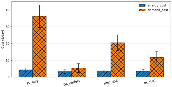
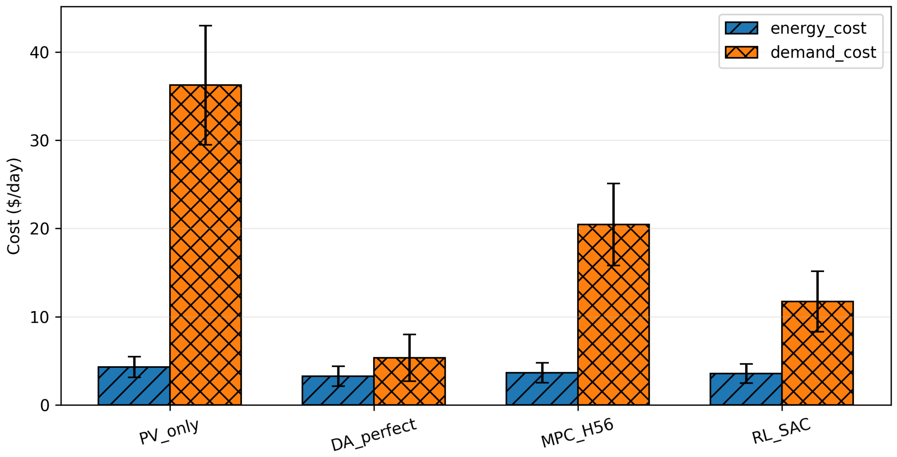
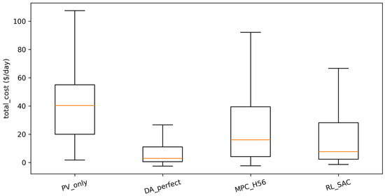
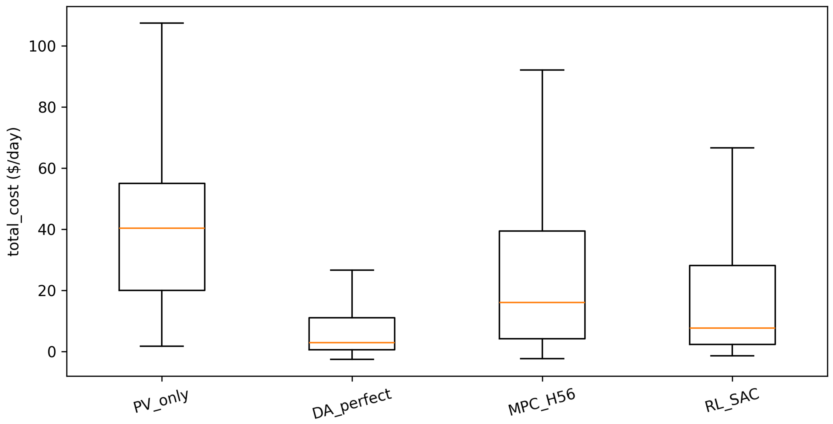
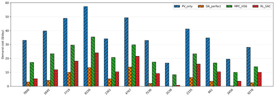
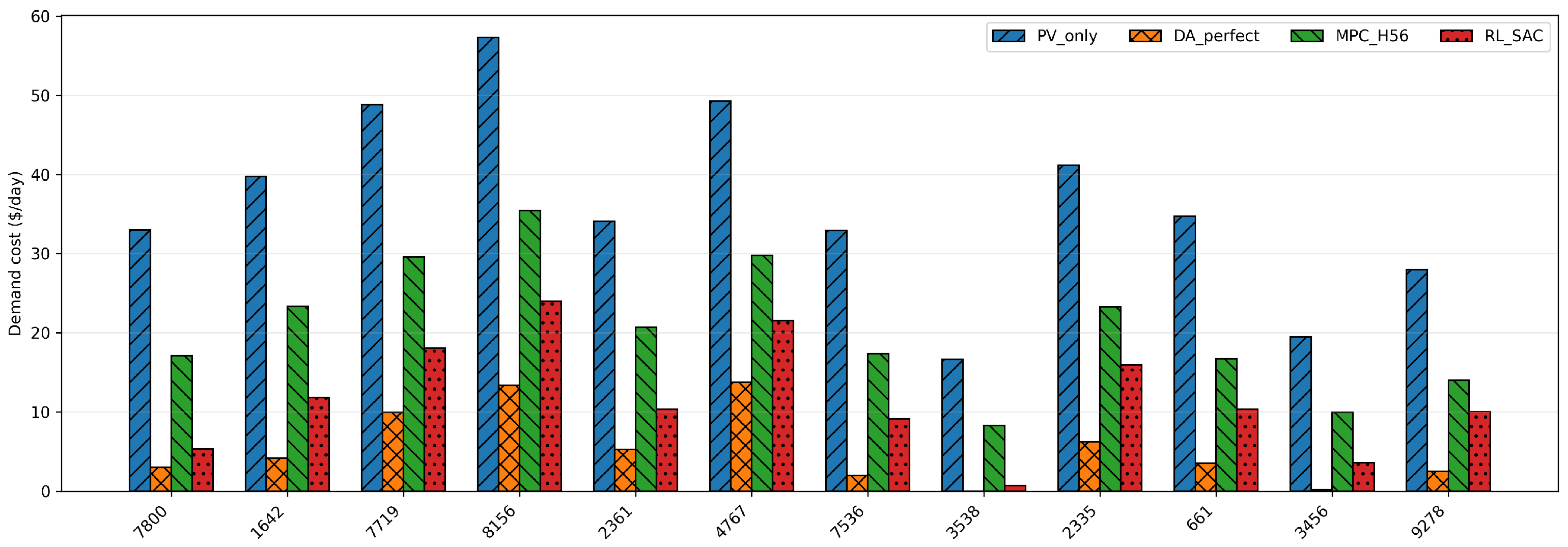
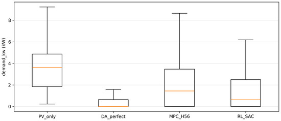
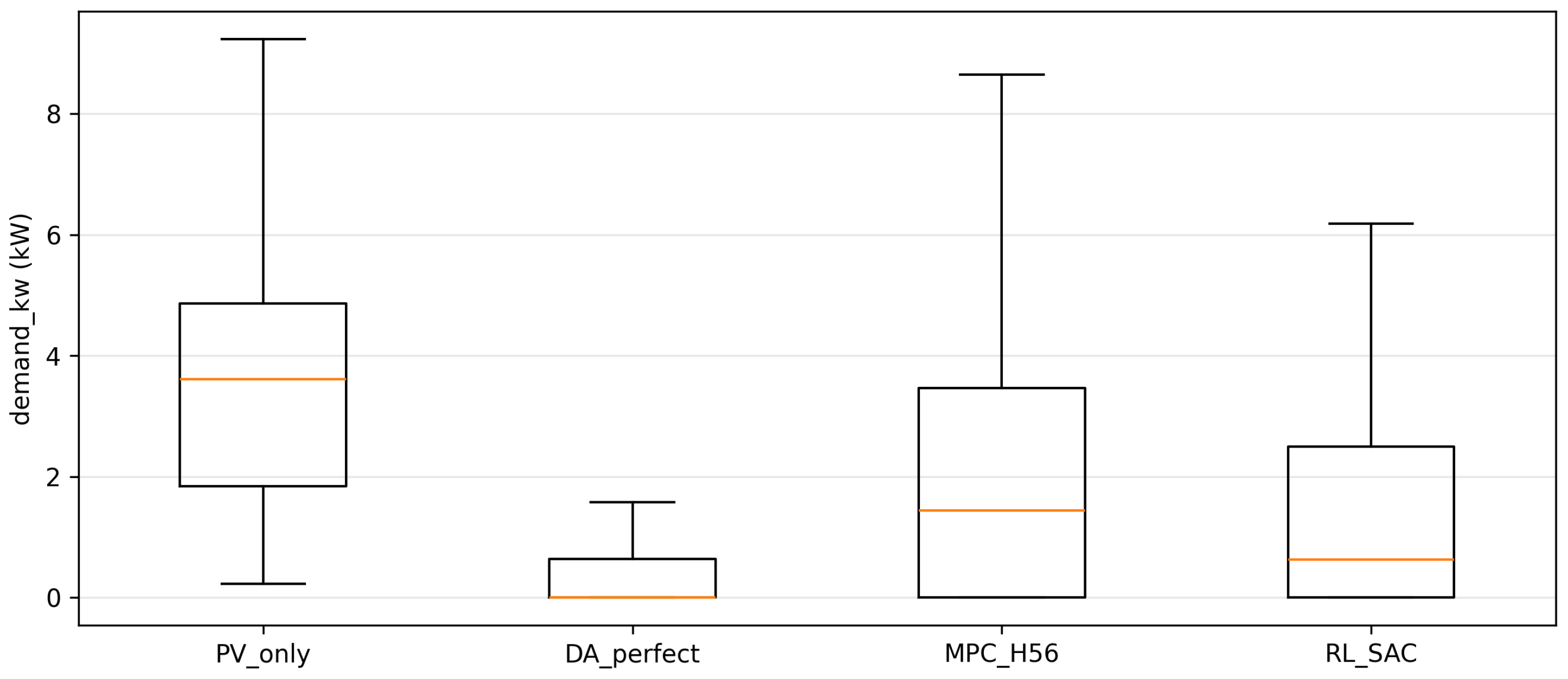
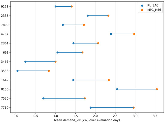
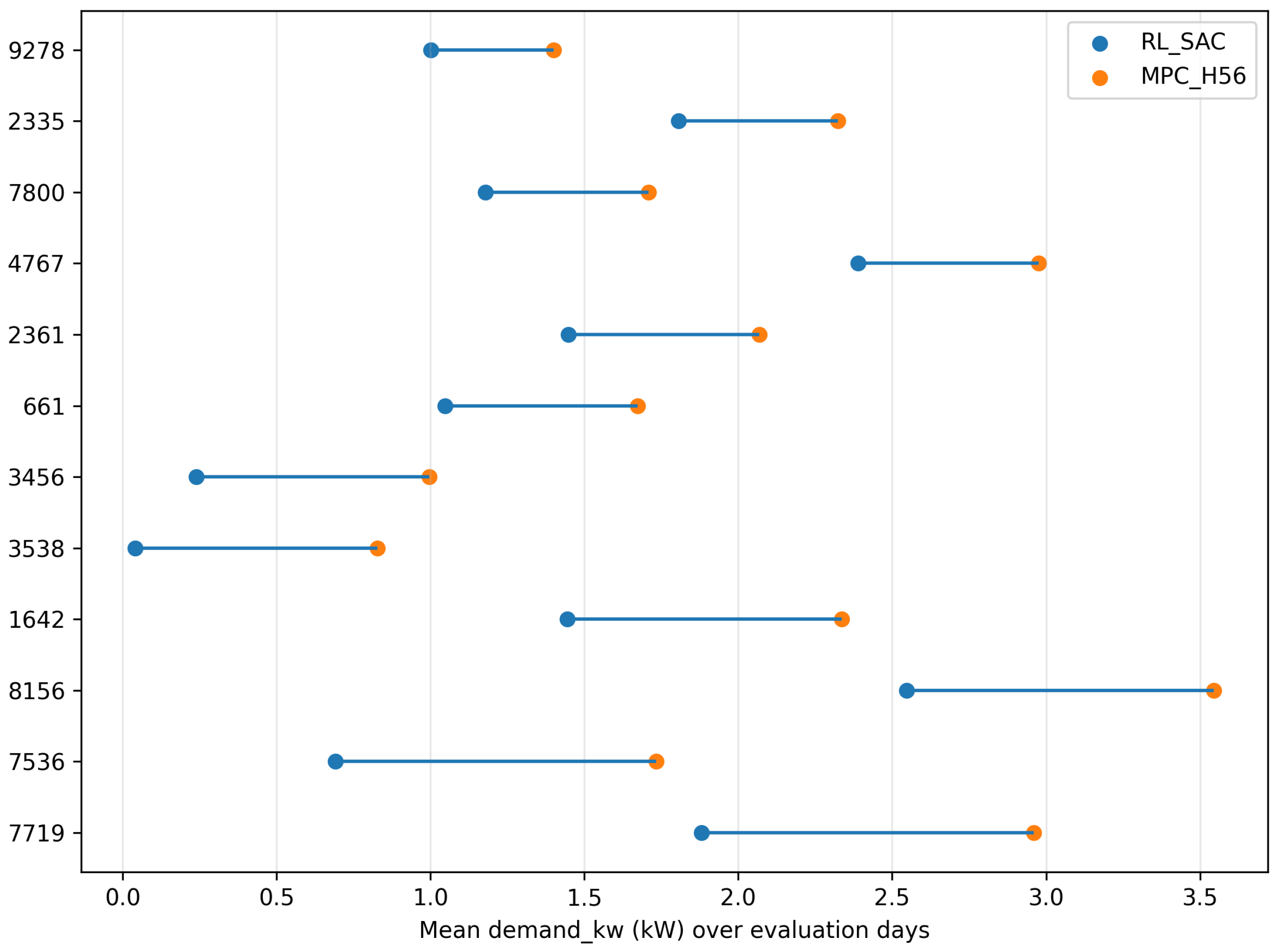
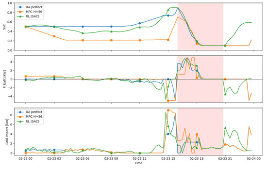
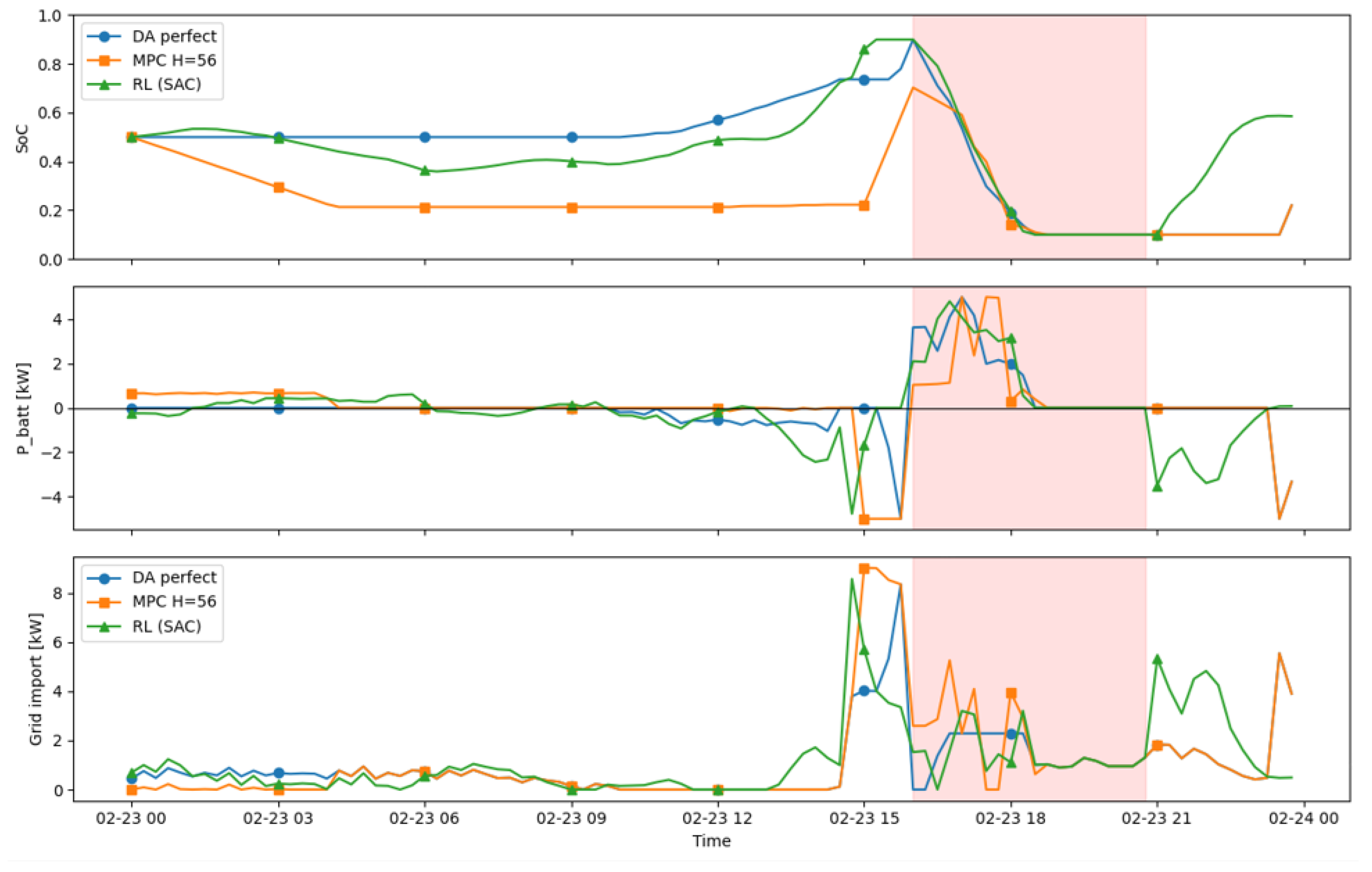
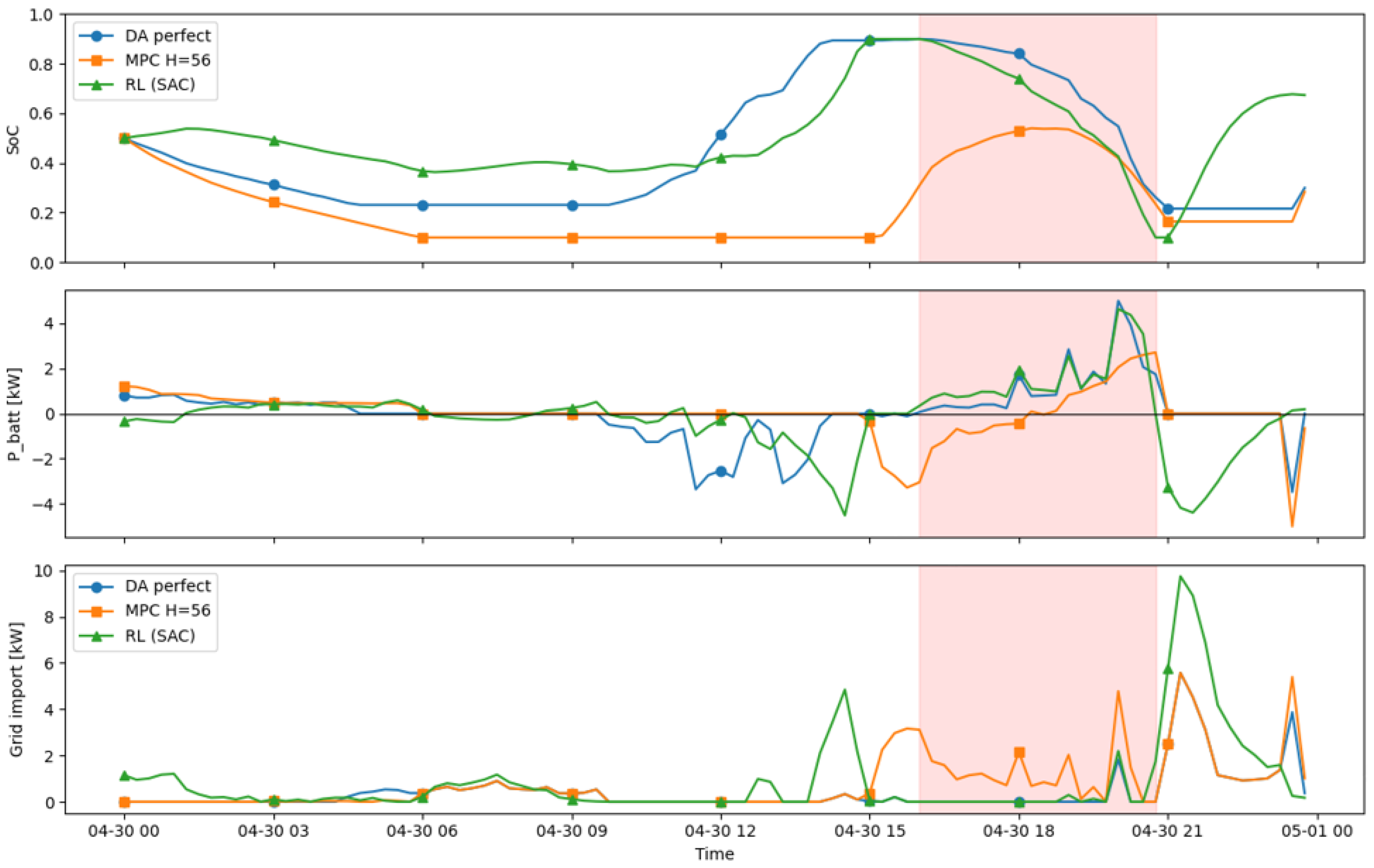
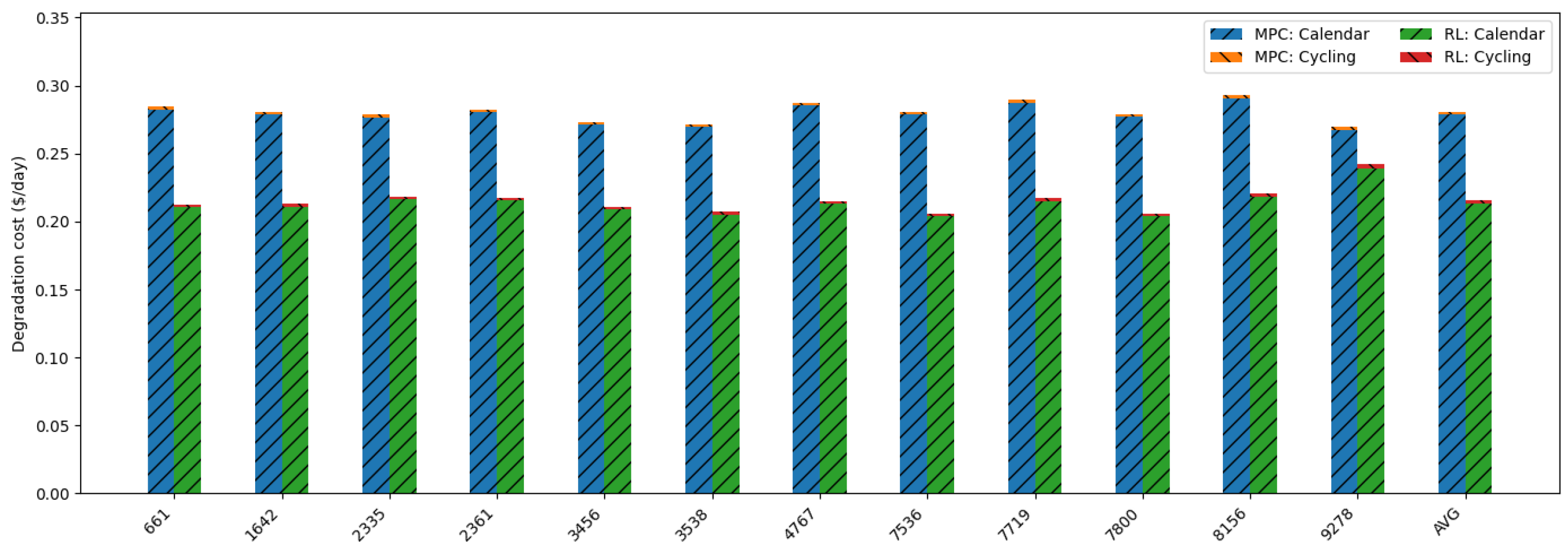
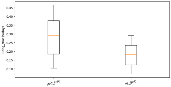
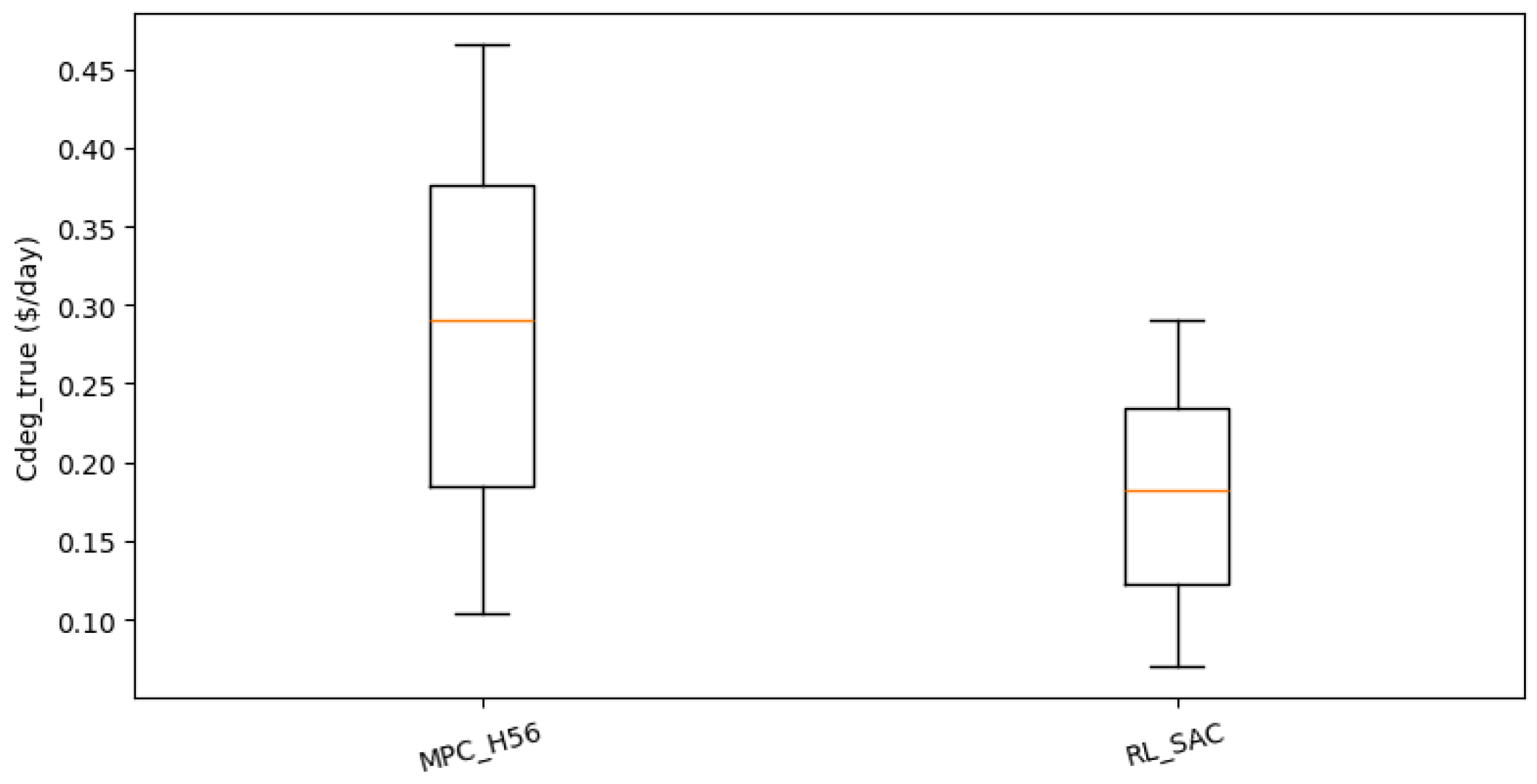
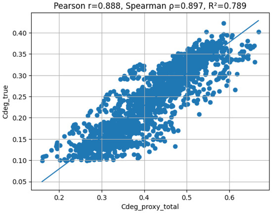
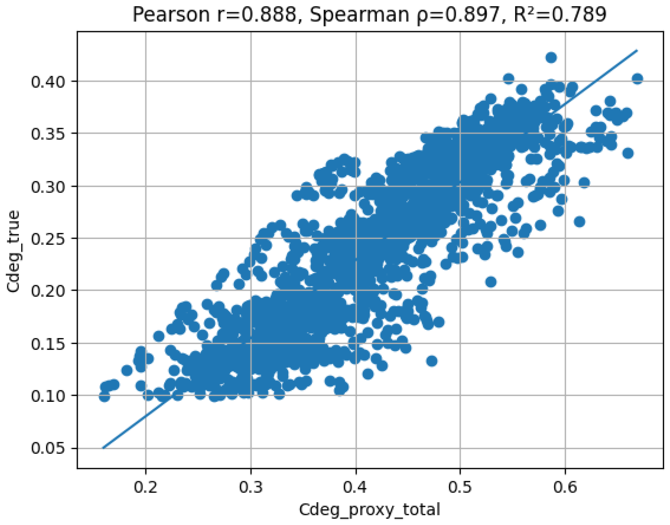

Disclaimer/Publisher’s Note: The statements, opinions and data contained in all publications are solely those of the individual author(s) and contributor(s) and not of MDPI and/or the editor(s). MDPI and/or the editor(s) disclaim responsibility for any injury to people or property resulting from any ideas, methods, instructions or products referred to in the content. |
© 2026 by the author. Licensee MDPI, Basel, Switzerland. This article is an open access article distributed under the terms and conditions of the Creative Commons Attribution (CC BY) license.