


Abstract
This paper discusses the problem of modeling heat transfer coefficient values in electronic circuits cooled by natural convection. This coefficient represents the heat exchange between the outer circuit surfaces and the surrounding environment, and in thermal simulations, their value is quite often assumed to be constant. However, in reality, it depends on both the absolute temperature of a surface and the temperature difference between this surface and the ambient. Consequently, this assumption may lead to important simulation errors, especially when a heat source occupies only a small part of the circuit’s area. This issue is illustrated here based on the results of thermal simulations carried out for a hypothetical test structure containing a heat source that dissipates different amounts of power, has variable dimensions, and is placed in various locations. Moreover, the thermal coupling between two heat sources is also analyzed as a function of their spacing. The simulation results are compared and analyzed for cases when the heat transfer coefficient value is constant and when it is temperature-dependent. The main conclusions of the analyses are that the simulated circuit temperature values are much lower when temperature-dependent values of the coefficient used and that proper optimization of the circuit layout could substantially decrease the maximal and average circuit temperature values.
1. Introduction
Thermal analysis of electronic circuits and systems is an essential part of the design process because thermal issues are the major cause of their malfunctions and failures. Usually, the temperature field inside a structure is described with the Fourier heat equation. For its solution, structure geometry and material thermal properties, as well as boundary or initial conditions, have to be specified [1,2,3]. Nevertheless, modeling the heat exchange with the surrounding ambient at a structure’s outer surfaces is not a trivial task. The natural convection cooling considered in this paper can be described with the set of Navier–Stokes partial differential equations [4,5,6], which have also been implemented in the most popular multidomain numerical simulation environments [7,8], with particular emphasis placed on natural convection [9,10].
However, using this heat transfer model may lead to unacceptably long simulation times. Thus, an attractive alternative is the application of Newton’s law of cooling at the structure’s outer surfaces, i.e., the Robin boundary condition. According to this law, the heat flux through a surface is proportional to the temperature difference between this surface and the surrounding ambient (fluid). The proportionality factor is normally called the heat transfer coefficient, but, again, the determination of the exact coefficient value is not straightforward and an averaged coefficient value in the form of a dimensionless number, such as the Nusselt number, is usually applied in thermal analyses [5,6,11,12].
Moreover, as pointed out in [13,14], these dimensionless relationships might not be true for electronic circuits containing tiny heat sources occupying just a small fraction of the entire structure surface area. Therefore, in reality, heat transfer coefficient values vary with surface temperature, hence their local values should preferably be taken into account. Otherwise, the obtained simulation results might yield significant errors. Consequently, other relationships based on empirical results should be used; for example, as was carried out by the authors of [15] for a tilted integrated circuit package. Other interesting solutions include the constructal theory [16,17] introduced by Bejan or the concept based on the characteristic length and the cooling circle developed by Luiten in [18,19,20,21]. However, the latter method uses the dimensionless Biot number, which is applicable only at a distance sufficiently far away from the heat source to consider its thermal response as one that decays exponentially in space, and it does not take into account local variations in heat transfer coefficient values.
Furthermore, the value of the heat transfer coefficient in thermal simulations is quite often assumed to be constant, with the value of 10 W/(m2 K) used as a ‘rule of thumb’ for natural convection [22]. As shown at a later point in this paper, this assumption may be correct only for temperatures just above the usual ambient temperature. Otherwise, local heat transfer coefficient values may vary significantly. This problem is described in this paper in detail based on the results of thermal simulations performed for a hypothetical test structure resembling a hybrid electronic circuit. The following section presents the thermal model of the structure, including the model used for the calculation of the heat transfer coefficient values. Finally, the thermal simulation results obtained in different simulation scenarios, with different locations and sizes for the heat source, are presented and discussed, providing indications for further research.
2. Hybrid Circuit Thermal Model
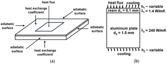
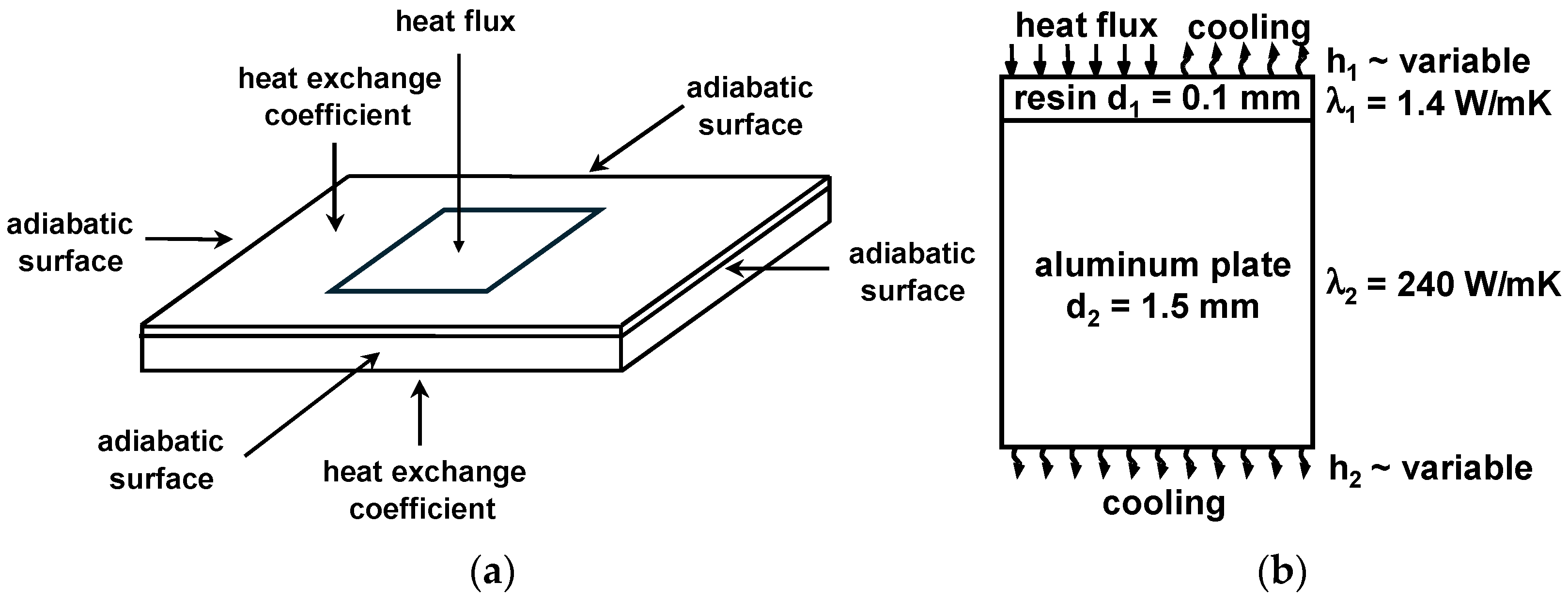
The thermal simulations presented in this paper were carried out for the structure pictured in Figure 1a, which resembles an electronic power module manufactured using insulated metal substrate hybrid technology. This structure consists of two layers: the base made of a 1.5 mm thick aluminum substrate with high thermal conductivity, and this is covered with a 100 μm thin resin insulating layer. The contact between the layers is assumed to be perfect, i.e., there is no temperature difference across the interface.
Figure 1.
Test circuit thermal model: (a) Imposed boundary conditions; (b) thermal parameter data.
The model takes into account the power dissipated into the heat source based on the heat flux flowing through its upper surface (the Neumann boundary condition), and the generated heat is exchanged with the ambient through the top and bottom surfaces according to Newton’s cooling law (the Robin boundary condition), characterized by the heat transfer coefficient, the value of which is variable and consistent with the model provided below. Furthermore, taking into account that the structure is relatively thin in comparison to its area, it could be assumed that the lateral surfaces are adiabatic, which implies the homogenous boundary condition of the second kind. Moreover, the thermal parameter data used in the simulations are given in Figure 1b.
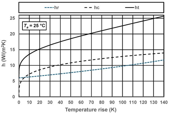
The heat transfer coefficient in this thermal model represents two different physical phenomena: radiation and convection. Radiation occurs when the surface temperature is higher than absolute zero, whereas convection appears if a temperature difference exists between this surface and the surrounding ambient. Since both cooling mechanisms typically occur at the same time, they are normally represented in thermal models by a single value, the total heat transfer coefficient ht, which is the sum of the radiation heat transfer coefficient hr and the convection heat transfer coefficient hc. The value of the radiative component hr depends on the surface’s absolute temperature T and the ambient’s absolute temperature Ta, whereas the convective component hc is proportional to the circuit’s surface temperature rise over the ambient temperature ΔT. These relationships are represented in Equations (1)–(3), where σ is the Stefan–Boltzmann physical constant and α is a constant found empirically. Here, the value 4.06 was used, as determined in [23] for a hybrid electronic circuit containing several power transistors. Alternatively, a unified heat transfer coefficient value taking into account both cooling mechanisms, as in [24], could be considered.
Ht = hr + hc
hr = σ × (T + Ta) × (T2 + Ta2)
hc = α × ΔT0.25
The actual value of the constant α depends, among others, on the orientation of the PCB (horizontal/vertical), its side (top/bottom), or surface flatness (build-up/plain). Regarding the effective value of thermal resistance from a surface to the ambient Rth, this is proportional to (1/(hr + hc)). Thus, its relationship to the total heat transfer coefficient value is nonlinear. Consequently, the dependence of the temperature rise on the dissipated power is also a nonlinear function.
The values of the total heat transfer coefficient ht, and both its components computed using the above equations for different values of surface temperature rise and an ambient temperature of 25 °C, are plotted in Figure 2. As can be seen, the value of the radiative component hr gradually increases from 6.0 W/(m2 K) to 9.8 W/(m2 K) for a temperature rise of 100 K over the ambient, whereas the value of the convective component hc rapidly grows to 12.8 W/(m2 K). Consequently, the value of the total heat transfer coefficient increases from 6.0 W/(m2 K) at the ambient temperature to 22.6 W/(m2 K). Hence, it increases more than three times. This fact, as demonstrated in the following section of this paper, has an important influence on the results of thermal simulations.
Figure 2.
Dependence of the heat transfer coefficient value on the circuit surface’s temperature increase.
3. Simulation Results
3.1. Simulation Settings and Tools
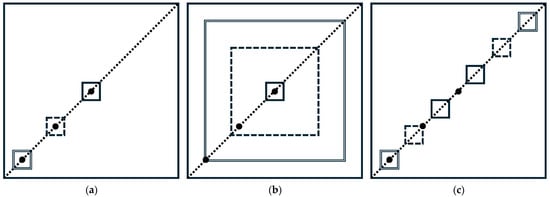
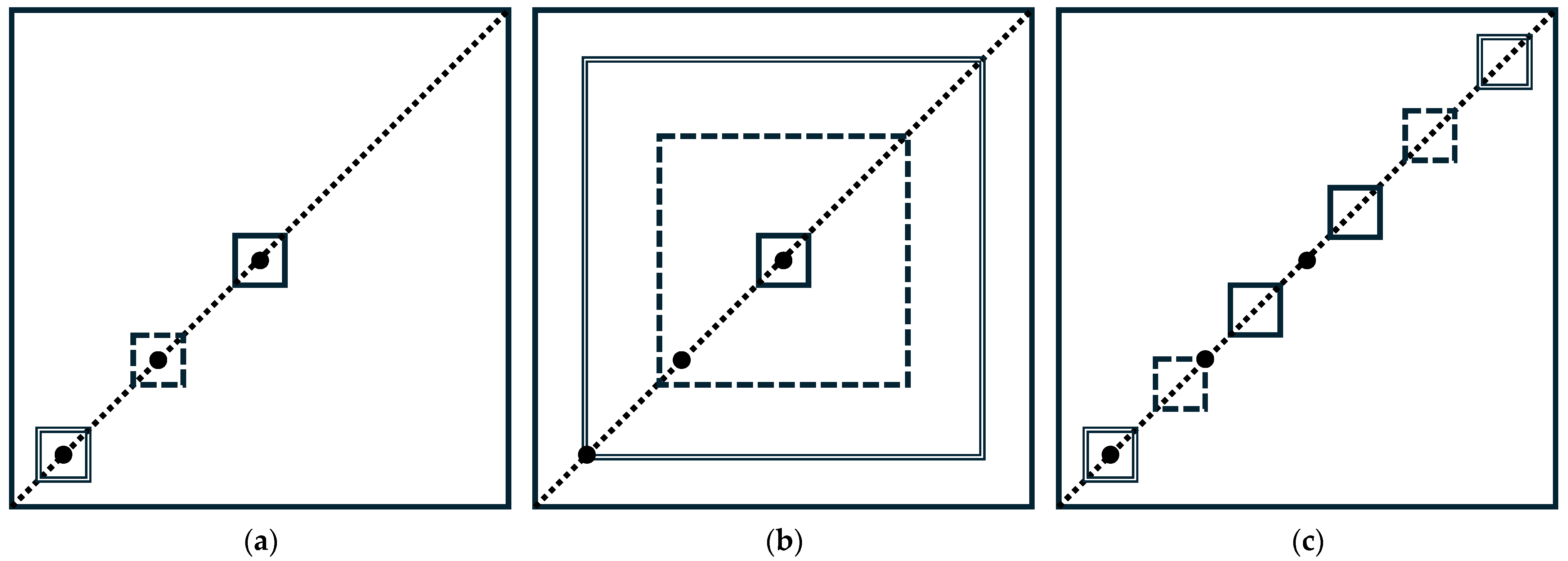
The electronic circuit layout analyzed in the thermal simulations presented in this paper resembles a real hybrid power module with lateral dimensions of 10 cm × 10 cm. Figure 3 summarizes all of the considered simulation scenarios. During the simulations, temperature values were read either along the diagonal of the circuit, represented by the dotted lines, or in the three locations indicated in the figure by large black dots (the very center, 3 cm from each edge and 1 cm from each edge). Initially, the influence of the heat source’s location and its size was studied. Then, the thermal coupling between two heat sources, as a function of their spacing, was investigated.
Figure 3.
Test circuit layout for different simulation scenarios: (a) Variable heat source location; (b) variable heat source size; (c) variable heat source spacing.
First, the location of a 1 cm × 1 cm square heat source was varied along the diagonal, as pictured in Figure 3a, so that the center of the source always coincided with one of the previously mentioned locations marked with the dots. Then, the size of the square heat source located in the center of the layout was varied so that it occupied 1% (solid line), 25% (dashed line) and 64% (double line) of the total surface area, as indicated in Figure 3b. Finaly, the thermal coupling between two 1 cm × 1 cm heat sources was studied at different spacings, as represented in Figure 3c. The spacings in both directions are 1 cm (solid lines), 4 cm (dashed lines) and 7 cm (double lines), respectively. All of the cases considered in the simulations are distinguished in the figure by solid, dashed and double lines.
The circuit temperature values were computed using the Green function analytical method. The main advantage of using an analytical heat equation method compared to a numerical method, such as the finite difference or element method, is that temperature values can be computed in selected locations of interest, so there is no need to solve a large set of equations, since the solution is given in the form of an explicit analytical formula.
Theoretically, Green’s functions can be used only for the solution of linear problems; however, when a nonlinearity originates from boundary conditions, as is the case here, this solution method can still be used [25]. Green’s functions are useful mathematical tools that can be regarded as transient temperature responses at a location of interest caused by the instantaneous generation of heat at another point; thus, a temperature response in time can be found by integrating a Green function over the entire volume and time of heat generation. Alternatively, Green’s functions are transient temperature responses at a point due to the initial temperature rise at another location. Then, the temperature evolution in time can be computed as the integral of this Green function, evaluated at the initial time instant over the entire domain of analysis.
Here, Green’s function was determined using the Fourier separation of variables method. More information on different methods for obtaining the temperature solutions of Green’s function can be found in [26,27], and the specific solution of the heat equation resulting from the proposed thermal model can be found in [28]. Solutions of Green’s function were calculated using the thermal solver implemented in the MathWorks MATLAB® simulation software (2020b). When the variable heat transfer coefficient was used, the solutions were obtained by iteratively updating the coefficient value based on the computed local surface temperature values. In order to obtain an accuracy of 0.01 K, four to nine iteration steps were required.
3.2. Influence of Heat Source Location and Size
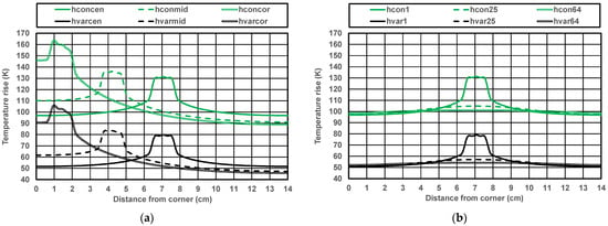
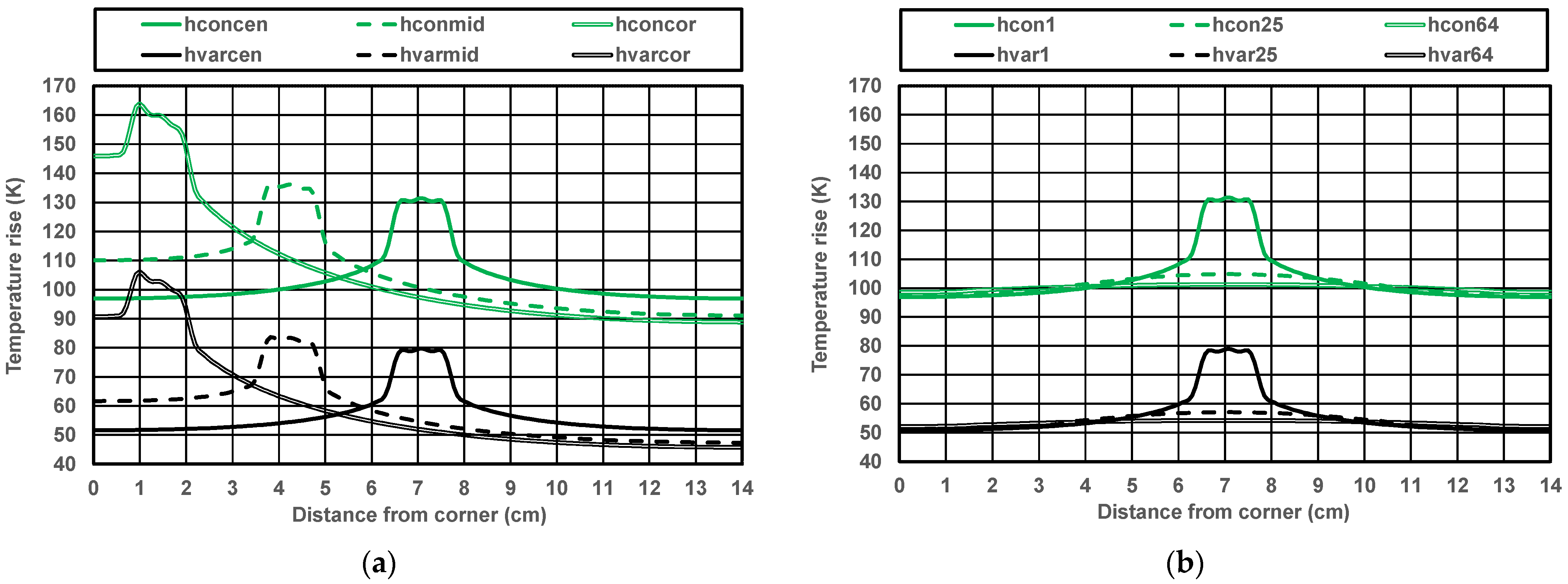
Initially, assuming a power dissipation of 20 W, the temperature rise profiles were computed along the diagonal of the circuit for three previously defined heat source locations, using either a constant heat transfer coefficient value equal to 10 W/(m2 K) or the local variable value computed based on Equations (1)–(3) for an ambient temperature of 25 °C. The results are plotted in Figure 4a, applying the same line types as in Figure 3a for each case. As can be seen, with the constant coefficient value (green lines), the source temperature rise varies from 131.4 K when the source is placed in the center (hconcen) to 163.8 K for the corner location (hconcor) and from 96.9 K to 88.8 K in the coolest location. With the temperature-dependent heat transfer coefficient (black lines), the respective temperature values are 79.0 K (hvarcen), 106.1 K (hvarcor), 50.8 K and 45.8 K. Thus, they are noticeably lower. Furthermore, with the constant heat transfer coefficient value, the temperature differences change from 34.5 K for the central source location to 75.0 K when the source is placed in the corner. With the variable coefficient value, these values are 28.2 K and 60.3 K, respectively. Thus, the temperature profiles are flatter when variable heat transfer coefficient values are used, and then temperature differences are lower by around 20%. Regarding the circuit layout, placing the heat source close to the corner increases its temperature by as much as one-third when the variable heat transfer coefficient value is used.
Figure 4.
Comparison of temperature profiles along the diagonal of the circuit with constant and variable heat transfer coefficient values for (a) different locations of a heat source occupying 1% of the circuit’s surface area, and (b) a centrally located heat source with a variable surface area.
Next, still assuming that the dissipated power is equal to 20 W, temperature increase profiles were computed along the diagonal of the circuit, as pictured in Figure 3b, for a heat source located in the center and of different dimensions, again using the constant and variable heat transfer coefficient values. The simulation results are plotted in Figure 4b. This time, with the constant coefficient value, the hot spot temperature varies from 131.4 K (hcon1) for the smallest heat source to 101.3 K for the largest one (hcon64), and from 96.9 K to 98.6 K in the coolest location.
With the variable coefficient, these values amount to 79.0 K (hvar1), 54.2 K (hvar64), 50.8 K and 52.1 K, respectively. Thus, they are again all noticeably lower. With the constant heat transfer coefficient, the temperature differences in the structure change from 34.5 K for the smallest heat source to just 2.7 K for the largest one. When the coefficient value is variable, these differences are equal to 28.2 K and 2.1 K. Hence, when the size of the source increases, the temperature across the circuit becomes more uniform.
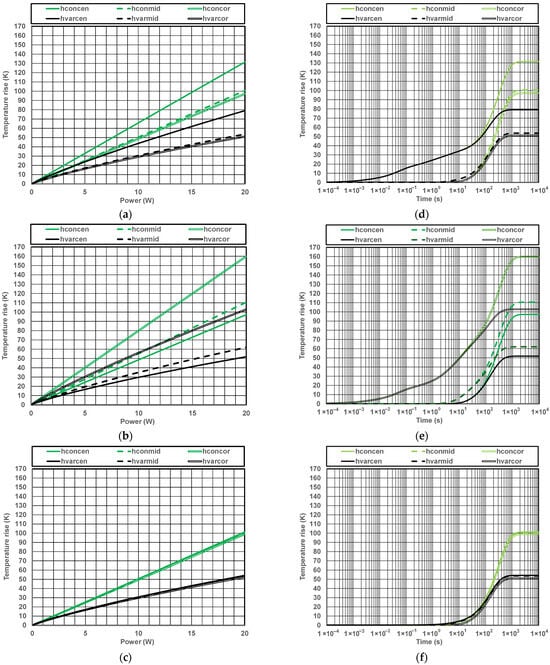
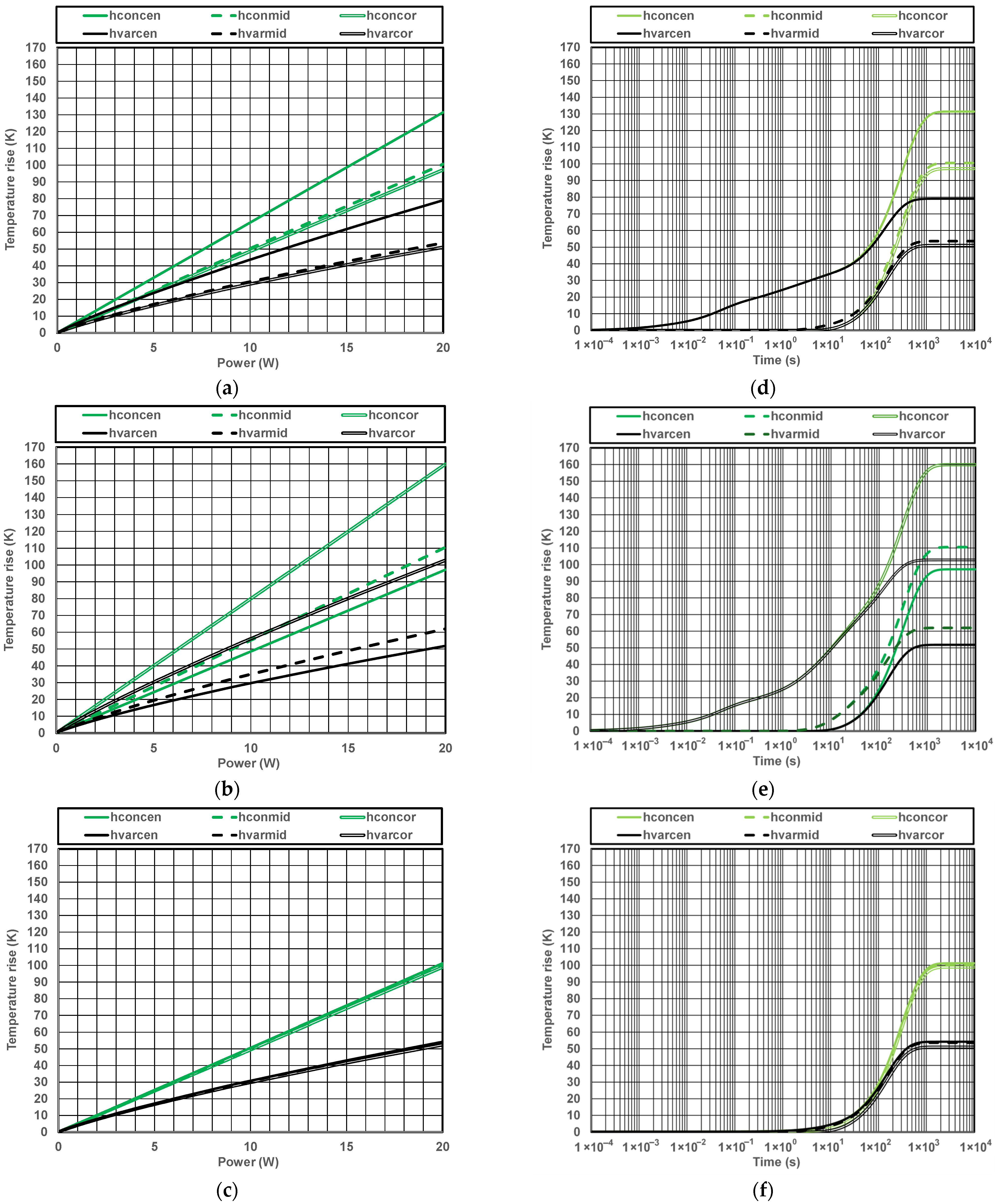
The next stage of thermal simulations investigated the impact of nonlinearities introduced by the heat transfer coefficient variable. For this purpose, the simulations were repeated with the power dissipated into the heat source varying from 100 mW to 20 W. The results obtained for selected cases from Figure 4—i.e., with the small source placed in the center or close to the corner, and with the largest source positioned in the center—are shown in Figure 5a–c (left column). The temperature values were simulated in the locations indicated by the black dots in Figure 3, and they correspond to the center (solid line), the intermediate location (the dashed line) and the corner point (the double line), respectively. These results again were obtained by applying either the constant heat transfer coefficient value (equal to 10 W/(m2 K) (green lines)) or the variable values consistent with the thermal model (black lines). Moreover, in order to facilitate the comparison of the figures, all of them have the same temperature scale on both axes.
Figure 5.
Temperature rise values at selected locations: (a) dependence on dissipated power for a heat source located in the center and occupying 1% of the circuit’s surface area; (b) dependence on dissipated power for a heat source located in the corner and occupying 1% of the circuit’s surface area; (c) dependence on dissipated power for a heat source located in the center and occupying 64% of the circuit’s surface area; (d) transient responses for a heat source located in the center and occupying 1% of the circuit’s surface area; (e) transient responses for a heat source located in the corner and occupying 1% of the circuit’s surface area; (f) transient responses for a heat source located in the center and occupying 64% of the circuit’s surface area.
As can be seen in the figures, when the value of the heat transfer coefficient is variable, the black lines depart from the green ones from the very beginning as a result of decreasing thermal resistance. Then, for 20 W of power dissipated into the heat source, the values of the temperature increase predicted for the cases considered by the thermal model with a variable coefficient are lower by 39.9%, 35.2%, and 56.5%, respectively. These differences are even more pronounced for locations outside the source, where the temperature values simulated using the variable heat transfer coefficient value are almost halved compared to the case when it is constant. Moreover, as can be seen from Figure 5c, for the large source, the temperature differences between the considered locations decrease and approach the one-dimensional limits, i.e., 100.0 K for the constant heat transfer coefficient value and 53.3 K for the variable one. This confirms that varying the heat transfer coefficient value with temperature significantly influences the simulation results. Hence, this should be always taken into account in thermal simulations of circuits cooled via natural convection.
Then, dynamic temperature responses were computed in three locations, corresponding to the ones presented in the left column, again assuming that 20 W of power was dissipated into the heat source. The computed curves representing the evolution of temperature over time are plotted in Figure 5d–f. A logarithmic time scale was used for the horizontal axes of the figures so as to better observe the process of heat diffusion as heating begins. In addition to the previously established fact that the steady-state temperature values are much lower when the coefficient value is variable, one can also observe that the temperature settling time is shorter—it is around a quarter of an hour for the variable heat transfer coefficient, and almost half an hour when the coefficient value is constant.
Another important conclusion is that the heating curve for the small heat source has a distinctly different shape because its temperature begins to increase after just a couple of milliseconds. Beyond the heat source, the thermal responses are delayed by a few seconds (see Figure 5d,e). For the larger heat source, this takes almost a second since the circuit substrate under the source has to be heated first (see Figure 5f). Furthermore, the influence of the variable heat transfer coefficient values becomes visible only after a couple of minutes. These results confirm that the transfer coefficient values have an important impact on the results of dynamic thermal simulations, and their variation with structure surface temperature should always be taken into account. Deeper analyses that consider the location and dimensions of the heat source can be found in [29,30].
3.3. Investigation of Heat Source Thermal Coupling
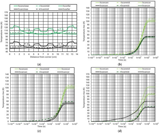
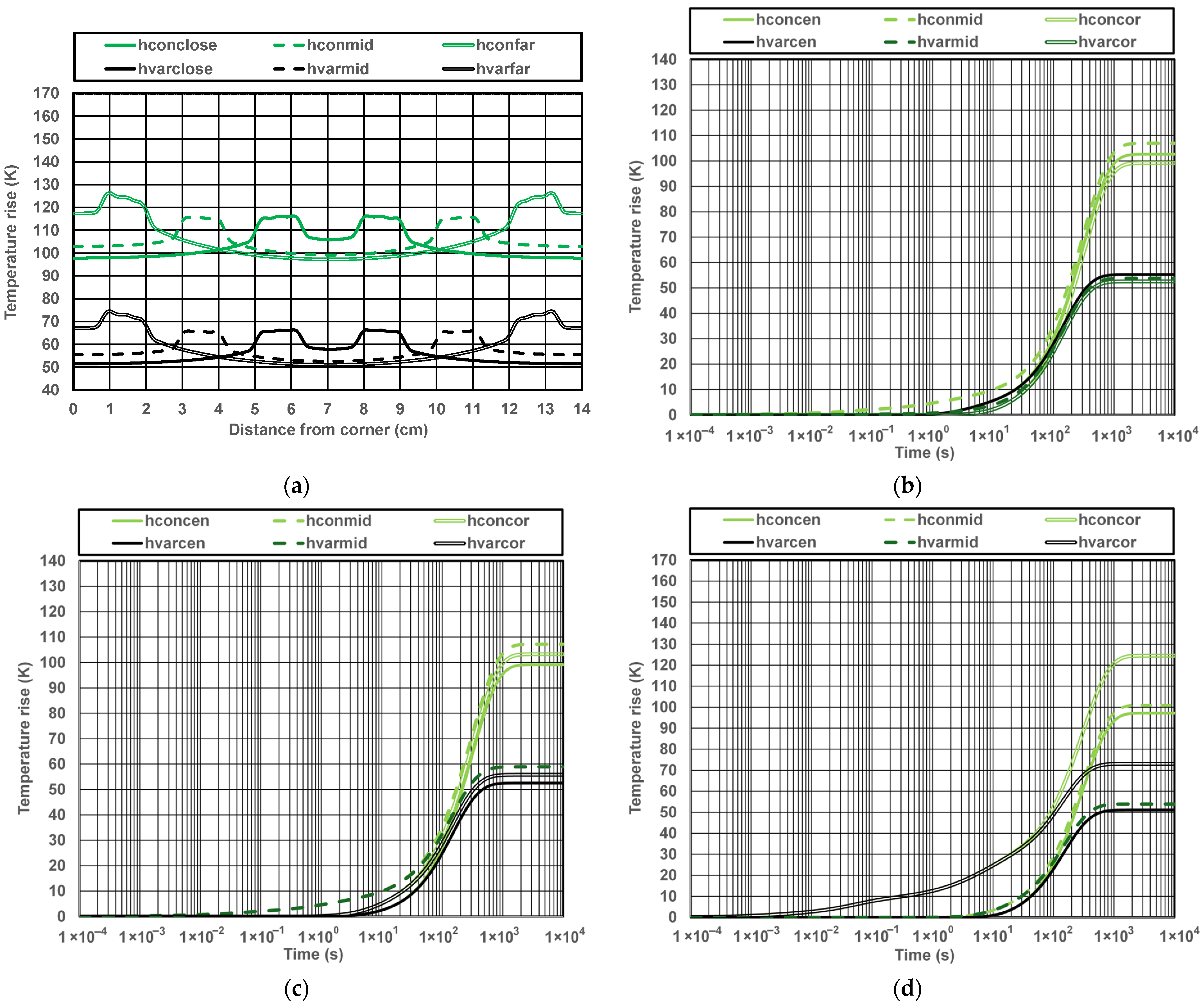
The last set of simulations presented here was devoted to investigating the influence of the value of the heat transfer coefficient on thermal coupling between two heat sources, each of them dissipating 10 W. During the simulations, as presented in Figure 3c, three different spacings were considered. The static temperature rise profiles computed for the cases considered here are plotted in Figure 6a. As can be seen, with the constant coefficient value, the maximal heat source temperature rise values vary from 126.4 K, when the sources are close to the corners, to 115.6 K for the intermediate spacing. On the other hand, when the sources are placed closer together, the maximal temperature value increases to 116.2 K due to the thermal coupling between the sources. With the variable coefficient, these values are again much lower, being equal to 74.6 K, 65.9 K and 66.3 K, respectively.
Figure 6.
Simulated temperature values for two heat sources, each of them occupying 1% of the circuit’s surface area and dissipating 10 W: (a) Static temperature profiles along the diagonal of the circuit; (b) dynamic temperature responses for closely located sources; (c) dynamic temperature responses for intermediate heat source spacing; (d) dynamic temperature responses for distant heat sources located close to the circuit’s corners.
Furthermore, it can be seen from the figure that, when the sources are distant, the coolest location is the center of the structure (97.2 K or 51.0 K), but when they are close to each other, the lowest temperature value is in the corner (97.8 K or 51.5 K). For the constant heat transfer coefficient, the temperature differences in the structure change with the decreasing source spacing, and they amount to 29.2 K, 16.5 K and 18.4 K, respectively. When the coefficient value is variable, these temperature differences are equal to 23.5 K, 13.3 K and 14.9 K. Thus, it can be concluded that an optimal source spacing should exist where the temperature difference is minimal and the temperature distribution is as uniform as possible.
Compared to Figure 4a, splitting the dissipated power between two heat sources can reduce the maximal temperature rise value by as much as 30%. Regarding the results of dynamic simulations shown in Figure 6b–d, they confirm all previous findings concerning the influence of the variable heat transfer coefficient value, the temperature settling time, and the delays in the response time of the heat source and of other locations.
4. Conclusions and Future Research
The main goal of this study was to assess the potential errors resulting from the use of a constant heat transfer coefficient value. The thermal simulations presented here demonstrate that, in the case of free convection-cooled electronic circuits, the value of the heat transfer coefficient cannot be regarded as constant. This is because in temperature ranges close to the ambient temperature, the value of this coefficient rapidly increases due to the sudden appearance of convection caused by the temperature difference between the circuit’s outer surface and the ambient. Consequently, the value of the convective coefficient already exceeds the value of the radiative one for a surface temperature increase of 5 K, and it becomes even more important in the range of temperature values normally encountered in electronic applications. The total value of the heat transfer coefficient already exceeds 20 W/(m2 K) for a surface temperature increase of 70 K over the ambient, making it two times greater than 10 W/(m2 K), which is the value typically assumed in thermal simulations for free convection.
Through the use of variable heat transfer coefficient values, it is possible to obtain accurate simulation results for all dissipated power values and at any location. Thermal simulations with variable heat transfer coefficient values yield much lower temperature values with visibly flatter profiles than those using a constant coefficient value. Therefore, local heat transfer coefficient values should always be taken into account for electronic circuits cooled via natural convection. Furthermore, the heat source temperature rise notably increases when located closer to the edges of the circuit. Regarding the size of the heat source, when it is considerably smaller than the circuit substrate, its temperature is noticeably higher than at the other locations. However, when it occupies just two thirds of the total circuit surface area, the temperature profile becomes fairly flat, and the temperature values approach the one-dimensional solution everywhere.
The simulations investigating thermal coupling between two heat sources demonstrate that dividing the total dissipated power among several sources could indeed effectively reduce circuit temperature. Moreover, the spacing between sources affects both the maximal circuit temperature rise and temperature differences, so further research could focus on optimizing source spacing to obtain a relatively uniform temperature distribution. The proposed method can also be employed for temperature-aware placement of components in circuit layouts, as in [31], so as to decrease the maximal temperature. Furthermore, the relationships between the average and local values of the heat transfer coefficient could be analyzed in greater detail.
Funding
This research received no external funding.
Data Availability Statement
The original contributions presented in this study are included in the article. Further inquiries can be directed to the corresponding author.
Conflicts of Interest
The author declares no conflicts of interest.
References
- Fourier, J.B.J. Théorie Analytique de la Chaleur; Firmin Didot: Paris, France, 1822. [Google Scholar]
- Carslaw, H.S.; Jaeger, J.S. Conduction of Heat in Solids, 2nd ed.; Clarendon Press: Oxford, UK, 1959. [Google Scholar]
- Hahn, D.W.; Ozisik, M.N. Heat Conduction, 3rd ed.; John Wiley & Sons Inc.: Hoboken, NJ, USA, 2012. [Google Scholar]
- Incropera, F.P.; De Witt, D.P.; Bergman, T.L.; Lavine, A.S. Principles of Heat and Mass Transfer, 8th ed.; John Wiley & Sons: Hoboken, NJ, USA, 2018. [Google Scholar]
- Holman, J.P. Heat Transfer, 10th ed.; McGraw-Hill: New York, NY, USA, 2010. [Google Scholar]
- Lienhard, J.H., V; Lienhard, J.H., IV. A Heat Transfer Textbook, 6th ed.; Phlogiston Press: Cambridge, MA, USA, 2024. [Google Scholar]
- Heat Transfer Modeling in Ansys Fluent. Available online: https://innovationspace.ansys.com/product/heat-transfer-modeling-in-ansys-fluent/ (accessed on 12 December 2025).
- Theory for the Heat Transfer Module. Available online: https://doc.comsol.com/6.3/doc/com.comsol.help.heat/heat_ug_theory.07.001.html (accessed on 12 December 2025).
- Natural Convection. Available online: https://innovationspace.ansys.com/product/natural-convection/ (accessed on 12 December 2025).
- Simulating Natural Convection in Air with COMSOL Multiphysics. Available online: https://www.comsol.com/blogs/simulating-natural-convection-in-air-with-comsol-multiphysics (accessed on 12 December 2025).
- Defining Heat Transfer Coefficient. Available online: https://innovationspace.ansys.com/courses/courses/topics-in-convective-heat-transfer-simulations/lessons/defining-heat-transfer-coefficient/ (accessed on 12 December 2025).
- Calculating the Heat Transfer Coefficient for Flat and Corrugated Plates. Available online: https://www.comsol.com/blogs/calculating-the-heat-transfer-coefficient-for-flat-and-corrugated-plates (accessed on 12 December 2025).
- Ellison, G. Thermal Computations for Electronics: Conductive, Radiative, and Convective Air Cooling, 2nd ed.; CRC Press: Boca Raton, FL, USA, 2020. [Google Scholar]
- Lasance, C. Sense and Nonsense of Heat Transfer Correlations Applied to Electronics Cooling. In Proceedings of the 6th International Conference on Thermal, Mechanial and Multi-Physics Simulation and Experiments in Micro-Electronics and Micro-Systems, Berlin, Germany, 18–20 April 2005; IEEE: New York, NY, USA, 2005; pp. 8–16. [Google Scholar] [CrossRef] [Scilit]
- Baïri, A. Free convective heat transfer coefficient for high powered and tilted QFN64 electronic device. Microelectron. Reliab. 2016, 66, 85–91. [Google Scholar] [CrossRef] [Scilit]
- Bejan, A. Constructal-theory network of conducting paths for cooling a heat generating volume. Int. J. Heat Mass Transf. 1997, 40, 799–816. [Google Scholar] [CrossRef] [Scilit]
- Bejan, A.; Lorente, S. Design with Constructal Theory, 1st ed.; John Wiley & Sons: Hoboken, NJ, USA, 2008. [Google Scholar]
- Luiten, G.A. Characteristic Length and Cooling Circle. In Proceedings of the 26th Annual IEEE Semiconductor Thermal Measurement and Management Symposium (SEMI-THERM), Santa Clara, CA, USA, 21–25 February 2010; IEEE: New York, NY, USA, 2010; pp. 7–13. [Google Scholar] [CrossRef] [Scilit]
- Luiten, G.A. Heat Spreading from a Small Source on A Thin Plate. In Proceedings of the 28th Annual IEEE Semiconductor Thermal Measurement and Management Symposium (SEMI-THERM), San Jose, CA, USA, 18–22 March 2012; IEEE: New York, NY, USA, 2012; pp. 275–282. [Google Scholar] [CrossRef] [Scilit]
- Luiten, G.A. Heat spreading in a thin longitudinal fin. Microelectron. J. 2014, 45, 539–546. [Google Scholar] [CrossRef] [Scilit]
- Luiten, W. Length Dimensions in Thermal Design. In Proceedings of the 24th International Workshop on Thermal Investigations of ICs and Systems (THERMINIC), Stockholm, Sweden, 26–28 September 2018. [Google Scholar] [CrossRef] [Scilit]
- Lasance, C. Basics of (PCB) Thermal Management for LED Applications. In Proceedings of the IPC APEX EXPO Technical Conference, Las Vegas, NV, USA, 12–14 April 2011. Paper E6&S09_02. [Google Scholar]
- Janicki, M.; Napieralski, A. Analytical Transient Solution of Heat Equation with Variable Heat Transfer Coefficient. In Proceedings of the 8th International Workshop on Thermal Investigation of ICs and Systems (THERMINIC), Madrid, Spain, 1–4 October 2002; pp. 235–240. [Google Scholar]
- Torzewicz, T.; Samson, A.; Raszkowski, T.; Sobczak, A.; Janicki, M.; Zubert, M.; Napieralski, A. Thermal Analysis of Hybrid Circuits with Variable Heat Transfer Coefficient. In Proceedings of the 33rd Thermal Measurement, Modeling and Management Symposium (SEMI-THERM), San Jose, CA, USA, 13–17 March 2017; IEEE: New York, NY, USA, 2010; pp. 19–22. [Google Scholar] [CrossRef] [Scilit]
- Gerstenmaier, Y.; Wachutka, G.K. Transient temperature fields with general nonlinear boundary conditions in electronic systems. IEEE Trans. Compon. Packag. Technol. 2005, 28, 23–33. [Google Scholar] [CrossRef] [Scilit]
- Beck, J.V.; Cole, K.D.; Haji-Sheikh, A.; Litkouhi, B. Heat Conduction Using Green’s Functions, 2nd ed.; CRC Press: Boca Raton, FL, USA, 2011. [Google Scholar]
- Greenberg, M.D. Application of Green’s Functions in Science and Engineering; Prentice-Hall: Englewood Cliffs, NJ, USA, 1971. [Google Scholar]
- Janicki, M.; De Mey, G.; Napieralski, A. Thermal analysis of layered electronic circuits with Green’s functions. Microelectron. J. 2007, 38, 177–184. [Google Scholar] [CrossRef] [Scilit]
- Janicki, M. Considerations on The Importance of Proper Modeling of Heat Transfer Coefficient Values. In Proceedings of the 32nd International Conference on Mixed Design of Integrated Circuits and System (MIXDES), Szczecin, Poland, 26–27 June 2025. [Google Scholar] [CrossRef] [Scilit]
- Janicki, M. Influence of Heat Source Dimensions and Heat Transfer Coefficient Value on Temperature of Electronic Circuits Cooled by Free Convection. In Proceedings of the 31st International Workshop on Thermal Investigation of ICs and Systems (THERMINIC), Naples, Italy, 24–26 September 2025. [Google Scholar]
- Cho, Y.; Kim, H.; Kim, H.; Kim, H.; Yoon, S.; Kim, I. Thermal Aware Floorplan Methodology Considering Heat Transfer Coefficient of Package to SOC Power Scenario. In Proceedings of the 24th IEEE Conference on Thermal and Thermomechanical Phenomena in Electronic Systems (ITherm), Dallas, TX, USA, 27–30 May 2025. [Google Scholar] [CrossRef] [Scilit]
Disclaimer/Publisher’s Note: The statements, opinions and data contained in all publications are solely those of the individual author(s) and contributor(s) and not of MDPI and/or the editor(s). MDPI and/or the editor(s) disclaim responsibility for any injury to people or property resulting from any ideas, methods, instructions or products referred to in the content. |
© 2026 by the author. Licensee MDPI, Basel, Switzerland. This article is an open access article distributed under the terms and conditions of the Creative Commons Attribution (CC BY) license.