


Abstract
This paper proposes a coordinated capacity configuration method for Virtual Power Plant (VPP) distributed resources that considers time-varying power coupling. The method addresses the inadequate economic efficiency and reliability of existing configuration schemes, which stems from insufficient attention to the time-varying power coupling characteristics of Distributed Energy Resources (DERs). Firstly, we define the concepts of direct and indirect power coupling among DERs, derive a Lagrange multiplier-based coupling coefficient model, and realize the quantification of time-varying coupling coefficients through sliding time window correlation analysis (STWCA). Next, a capacity correlation matrix integrating technical and economic synergies is constructed to map coupling characteristics to capacity configuration. Then, a coordinated configuration model with time-varying coupling constraints is established to minimize life-cycle cost and maximize power supply reliability, validated by case simulation. The results demonstrate that the proposed method effectively reduces VPP operation cost and improves resource utilization and reliability, providing theoretical support for the scientific configuration of DERs in VPPs.
1. Introduction
In the process of energy transition, the large-scale grid integration of Distributed Energy Resources (DERs) has become an inevitable trend in the industry development. However, the inherent characteristics of DERs, such as intermittency, randomness, and geographical dispersion, have led to prominent issues such as increased difficulty in power grid dispatching, severe curtailment of wind and solar power, and low resource utilization efficiency [1]. As the core carrier for the management of DERs, Virtual Power Plants (VPPs) can realize the coordinated control of DER clusters through advanced technical means, thereby functioning as a “virtual power generation unit” that deeply participates in power system dispatching, operation, and electricity market transactions. It is key to resolving the contradiction between DER accommodation and the safe operation of power grids [2,3]. Among the key links in VPP planning, capacity configuration is particularly critical [4], as it directly determines their economic efficiency and reliability during the operation phase [5]. Research on capacity configuration holds fundamental and pioneering significance for VPPs. Scientifically sound and rational configuration directly determines whether VPPs can fully leverage aggregation advantages and maximize the environmental and economic value of DERs [6]. Furthermore, it profoundly influences the safe and stable operation of power systems and the efficiency of resource optimization allocation [7,8]. Thus, it has become one of the core topics urgently requiring in-depth exploration in the current VPP field.
Existing theoretical research on VPP capacity configuration is mostly based on the idealized assumption of “decoupled operation” of DERs. The core research paradigm of this field focuses on the capacity optimization of a single energy storage component, and no systematic analysis framework considering the coupling characteristics of DER clusters has yet been established. For example, based on risk–return trade-off theory, Reference [9] established a user-side energy storage capacity configuration model considering dynamic time-of-use electricity prices and Conditional Value at Risk (CVaR), improving the constraint system for energy storage optimization from the perspectives of economy and risk controllability. Reference [10] proposed a hybrid energy storage capacity configuration strategy for virtual power plants based on variable-ratio natural gas–hydrogen blending, aiming to address issues such as power fluctuations in large-scale wind farms and wind curtailment accommodation. From the perspective of multi-objective trade-off among reliability, flexibility, and economy, Reference [11] established hierarchical capacity configuration criteria for wind–solar-storage VPPs. Although the above studies have deepened the optimization logic of single energy storage components, they all overlook the power coupling characteristics of DER clusters, which are determined by electrical topology constraints, energy conversion mechanisms, and coordinated control strategies, leading to deviations between theoretical models and the physical nature of actual VPP operations.
Some scholars have recognized this theoretical flaw and begun to attempt incorporating the power coupling relationships between DERs into research. Based on multi-energy flow coordination theory, Reference [12] proposed a multi-energy complementary operation framework suitable for commercial VPPs, initially establishing a capacity configuration logic under coupling relationships. Targeting the characteristics of wind–solar–hydrogen–thermal VPPs, Reference [13] constructed a capacity configuration model based on the wide power regulation capability of alkaline electrolyzers, making the coupling constraints of hydrogen conversion links explicit. However, such studies still have theoretical shortcomings—they all adopt constant coupling coefficients to construct constraint conditions, essentially treating dynamic coupling relationships as static ones. They fail to reveal the time-varying correlation mechanism between coupling strength and operating scenarios, as well as environmental parameters, resulting in models being unable to characterize the dynamic evolution characteristics of VPP operating states.
From the perspective of the physical nature of VPP operations, the power coupling between DERs exhibits significant time-varying characteristics [14], driven by both the randomness of renewable energy output and the volatility of load demand. Taking the coupling relationship between photovoltaic (PV) systems and Energy Storage Systems (ESSs) as an example, PV output shows strong volatility due to the dynamic influence of parameters such as intraday illumination intensity and atmospheric transparency, and the power interaction coefficient between PV and ESSs must be dynamically adjusted according to operating time periods. Neglecting this characteristic during capacity configuration leads to a mismatch between theoretical and actual operational requirements. This may not only cause capacity redundancy at the investment level but also result in insufficient regulatory capacity at the operational level, ultimately failing to support the construction of a precise capacity-coordinated configuration theory and engineering practice for VPPs based on dynamic coupling relationships. Therefore, this paper conducts research on the coordinated-capacity configuration of distributed resources in VPPs, considering time-varying power coupling. Firstly, the types and mechanisms of power coupling between DERs are analyzed, and a calculation method for time-varying coupling coefficients is proposed. Next, a capacity correlation matrix integrating technical and economic dimensions is constructed to realize the quantitative mapping from power coupling to capacity configuration. Then, a multi-objective coordinated capacity configuration model is established, and the feasibility and superiority of the proposed method are verified through numerical examples.
2. DER Time-Varying Power Coupling Quantification
2.1. Types and Characterization of Power Coupling
Due to the mutual constraints of electrical connections, energy conversion, and control strategies among DERs aggregated by VPPs, DERs exhibit complex nonlinear power coupling characteristics [15], including direct coupling and indirect coupling. Direct coupling refers to power interaction formed through physical grid connections—such as the power flow impact between different devices under the same busbar—which directly alters the power output of each other. Indirect coupling arises from associations induced by control strategies or energy conversion links. The power coupling of aggregated resources determines the overall performance of VPPs in energy dispatching and market response. Analyzing the coupling characteristics of VPP-aggregated resources is the basic premise for achieving effective DER aggregation [16].
Consider a VPP containing N DERs; its power coupling characteristics can be represented by a matrix as
Here, denotes the influence of the power variation of DER on DER . Following the coupling degree calculation principle of sensitivity analysis, and based on the Lagrange multiplier of the optimization model, the marginal impact of power variation between DERs is defined as the coupling coefficient , i.e.,
In this equation, the value of element ranges between −1 and 1, with the following implications:
- When , it indicates that there is no coupling relationship between resource and resource ;
- When , it indicates that there is a positive coupling relationship between resource and resource ; specifically, means that resource is only affected by resource ;
- When , it indicates that there is a negative coupling relationship between resource and resource .
For a VPP incorporating photovoltaic (PV), wind turbine (WT), micro turbine (MT), energy storage system (ESS), and adjustable load (L), all resources are connected to the same busbar. The power balance (i.e., the coupling relationship) satisfies
In this equation, is the real-time output of WT; is the real-time output of PV, with ; is the ESS power, where a positive value indicates discharging and a negative value indicates charging; is the load power, with ; is the grid interaction power, where a positive value indicates injecting into the grid and a negative value indicates drawing power from the grid; and denotes the line loss.
For ease of reference and to enhance the readability and clarity of this paper, all major mathematical symbols used in the study, together with their specific definitions and corresponding units, have been systematically organized and compiled in Table A1 of Appendix A.
2.2. Power Coupling Mechanism of Typical DERs
2.2.1. PV-WT and ESS Coupling
The power coupling characteristics between PV-WT generation and the ESS manifest in their energy interaction and electrical energy balance relationship [17]. The PV system is affected by fluctuations in light intensity, while the WT system is influenced by wind speed variations—both exhibit intermittency and randomness in output power. The ESS can mitigate PV power fluctuations and enhance system stability through charge–discharging regulation. Coupling coefficients and , respectively, reflect the direct impact of PV output power variations and WT output power variations on the charging power of the ESS. For example, when PV output increases by 1 kW, the ESS needs to increase its charging power by 1 kW accordingly under full accommodation conditions, so ; if curtailment of PV power is allowed in the system, the charging demand of the ESS can be reduced by adjusting the PV curtailment amount, so . Specifically, when PV output exceeds the load demand, the ESS prioritizes charging to accommodate the excess generation power; when PV output is insufficient, the ESS supplements the power gap by discharging.
Coupling coefficients and (for the coupling from ESS to PV-WT generation, respectively, reflect the indirect impact degree of the ESS’ charge–discharging behavior on the output power of PV and WT. This is mainly manifested as when the ESS absorbs power from the grid, PV or WT may need to curtail output or operate at a derated capacity; when the ESS is charging, to avoid overvoltage, WT may be derated . When , it indicates that the ESS has no impact on the operation of WT.
2.2.2. PV-WT and Generation-Adjustable Load Coupling
The power coupling characteristics between PV-WT generation and adjustable loads exhibit significant load type dependency [18]. The coupling mechanisms and quantification indicators vary notably across different load scenarios. The direct impact degree of PV-WT power variations on load demand reflects whether PV-WT generation can directly meet load demand or replace grid power supply. For example, for rigid commercial loads, lighting loads, and scheduled production loads, the load is not directly affected by PV at all, so in this case. For adjustable loads, the load can be dynamically adjusted based on PV-WT output: when PV or WT output is surplus, with energy accommodation as the priority, the excess power variation of PV or WT is fully absorbed by the load (while WT output is reduced synchronously), so and . When WT output is insufficient, with power supply as the priority, the reduction in WT output is partially offset by PV (or the power variation is fully absorbed by the load), so and . In addition, there is also indirect coupling between PV-WT generation and the load. For instance, in demand response regulation, excessively high PV-WT output may cause feeder voltage violation; in this case, adjustable load energy dissipation needs to be triggered to maintain voltage stability, so and under this condition.
The impact degree of load power variations on PV-WT operation reflects whether load demand changes lead to PV-WT curtailment or operation mode adjustment. When PV and WT always operate at maximum power, load variations do not affect PV-WT output, so and . When load decreases (resulting in PV-WT curtailment), or when load increases (prompting PV-WT to raise output), the coupling is a co-directional regulation, so and .
2.2.3. PV and WT Coupling
PV and WT, as the two major mainstream renewable energy sources, have complex coupling relationships in their coordinated operation within the power grid [19]. From the perspective of power interaction, the coupling between PV and WT reflects the direct impact of PV’s real-time power on the dispatched power of WT; this is a bidirectional interaction, mainly manifested in aspects such as power allocation in voltage regulation, and impacts on local power grid or frequency regulation. The typical operation mode is independent operation of the two, i.e., and ; under some extreme scenarios, the two are in competitive accommodation (with harmony degree < 0), i.e., ; in extreme cases (e.g., during high-wind periods), WT fluctuations trigger PV frequency regulation, so .
2.3. Quantitative Characterization and Dynamic Calculation of Time-Varying Power Coupling Coefficients
Based on the DER power coupling relationship described in Equation (1), the quantitative expression of power sensitivity can be expressed as Equation (4):
Here, , , , , and denote the power variations of WT, PV, micro turbine (MT), ESS, and load, respectively; , , , , and denote the initial power states of each resource; the diagonal elements in the coupling matrix indicate that distributed resources do not couple with themselves; the coupling matrix is asymmetric; and the off-diagonal elements characterize the coupling strength between different resources, with .
In practical scenarios, the power coupling of distributed resources changes with natural fluctuations (e.g., illumination, wind speed) and dynamic adjustments of grid dispatching strategies. Static coupling coefficients cannot adapt to this multi-time-scale dynamic characteristic; thus, the coupling coefficient needs to be extended as a function of time, denoted by to characterize its dynamic evolution.
Although the coupling coefficient is theoretically defined as a Lagrange multiplier (as shown in Equation (2)) to characterize the marginal impact of power changes, directly solving the time-varying Lagrange multiplier faces challenges such as complex models, a large computational load, and difficulty in accurately adapting to dynamic scenarios. To achieve time-window adaptive estimation of the coupling coefficient, this paper adopts the Sliding Time Window Correlation Analysis (STWCA) as its statistical estimation method: it captures the dynamic evolution of coupling relationships through a data-driven approach, which not only avoids the difficulty of solving complex models but also adapts to multi-time-scale dynamic characteristics. The theoretical basis is that during the quasi-steady-state period of system operation, the statistical correlation between DER power variables can approximately reflect their physical sensitivity. If it is assumed that the system maintains a quasi-steady state within the sliding time window and external disturbances (such as wind and solar fluctuations, load changes) have approximate continuity within the window, the correlation between the power sequences of resource and resource can approximately replace the time-varying estimation of their sensitivity, and the calculation formula is shown in Equation (5).
Here, is time instant variable within the sliding time window; is the width of the sliding time window; and and denote the average power of resource and resource within the time window, respectively.
The selection of window width is the key to balancing the model’s dynamic capture capability for fluctuation characteristics and the robustness of statistical estimation:
- An overly short window (e.g., 1 h) can respond quickly to power mutations, but it is susceptible to random noise interference, causing severe fluctuations in the coupling coefficient sequence and a large estimation variance;
- An overly long window (e.g., 24 h) can yield a smooth estimation, but it will over-average and fail to distinguish the differences in coupling relationships between wind–PV output and load during different intraday periods (e.g., daytime when PV output peaks and night when there is no PV output).
Considering the fluctuation cycle of typical wind–PV resources (on the order of several hours), the time scale of power system dispatching, and the experience of intraday fluctuation analysis in relevant studies, this paper selects w = 4 h as the baseline value. This is to capture the characteristics of typical intraday phases (such as “morning–afternoon–evening”) while obtaining a sufficiently stable statistical estimation.
3. Time-Varying Coupling-Integrated Capacity Correlation Matrix
The capacity correlation matrix extends power coupling characteristics to the capacity planning dimension. By quantitatively characterizing the long-term capacity configuration adaptation intensity of various distributed resources, it reflects the dynamic matching requirements between resources, and can reveal the synergistic support effect of different resource combinations on the reliability and economy of VPPs [20]. It serves as a core component in the optimal configuration of VPPs. By quantifying the techno-economic coupling relationships between DERs, it directly determines the capacity constraints and allocation strategies for each DER when the VPP participates in market transactions.
3.1. Basic Form of the Capacity Correlation Matrix
For a typical VPP configuration including PV, WT, MT, ESS, and L, its capacity correlation matrix can be expressed as
Here, the diagonal elements satisfy , which means that when the capacity of the -th resource is adjusted, its own capacity configuration needs to be adjusted synchronously. Off-diagonal elements characterize the capacity proportion that resource needs to adjust synchronously when the -th resource increases its capacity by 1 unit. Its numerical characteristics directly reflect the capacity coordination relationship between resources: the larger the absolute value, the stronger the capacity interlock between the two resources, and .
3.2. Calculation of Capacity Correlation Matrix Elements
The elements of the capacity correlation matrix are not empirical values but integrated quantitative results of the long-term operating characteristics of time-varying power coupling and the economic effects of resource capacity synergy. They serve as a “converter” for technical and economic constraints between DERs, with the core function of transforming dynamic power interactions at the “operation layer” into capacity adaptation constraints at the “planning layer.”
The element of the capacity correlation matrix consists of a technical capacity correlation term and an economic synergy term:
- The technical capacity correlation term is the effective integral average of power coupling over the long-term dimension, reflecting the cumulative impact of power interactions between resources on concurrent capacity demands. Its calculation requires evaluating the matching degree between equipment efficiency and operating time.
- The economic synergy term is the second-order gradient of power coupling in the cost dimension, quantifying the marginal effect of resource capacity changes on the system’s total cost.
The complete calculation formula for is expressed as
Here, denotes the effective integral average of the time-varying elements within the brackets; is the time-varying power coupling coefficient of resource to resource , which can be calculated using Equation (5); represents resource efficiency; is the utilization ratio of resource , where denotes the equivalent full-load hours of resource and is the effective operating hours of resource ; is the economic adjustment factor; and is the system total cost function, while and represent the capacity configurations of resource and , respectively.
The economic synergy term quantifies the cross-impact of resource capacities on the system’s total cost, reflecting economic synergy or competition effects. This paper adopts the black-box simulation method to calculate the second-order mixed partial derivative of the cost function; thus, the economic synergy value can be discretely approximated as
Here, denotes the system cost, and is the capacity perturbation step size; typically, is set to 5–10% of the system rated capacity.
To ensure the objective weight allocation between technical and economic terms in capacity correlation, and avoid overfitting of subjective parameters, we define using weighted fitting normalized by the overall system operation data. Specifically, the value of β is determined by the ratio between the average value of all elements in the technical capacity correlation term matrix and the average absolute value of all elements in the economic synergy term matrix, as calculated in Equation (9).
This method transforms the determination process of from “manually preset parameters” to “data-driven calculation”. Its physical significance lies in reflecting the inherent relative strength of technical constraints and economic effects as exhibited in long-term operation data, thus ensuring the unbiasedness and reproducibility of parameter selection.
4. Time-Varying Coupling-Integrated Capacity Coordination Model
Based on the analysis of time-varying power coupling characteristics and the construction of the capacity correlation matrix, this paper takes the techno-economic-reliability synergy in the life-cycle of the VPP as the core, and constructs a capacity-coordinated configuration model considering time-varying coupling constraints to achieve accurate matching of resource capacities.
4.1. Multi-Objective Function
This paper establishes dual optimization objectives: minimizing VPP life-cycle cost and maximizing power supply reliability. The linear weighted normalization method is adopted to eliminate dimensional differences, converting the multi-objective problem into a single-objective optimization problem. It can be specifically expressed as
Here, and denote the life-cycle cost and load deficit rate, respectively; and are objective weights, satisfying .
For the full-life-cycle cost , its ideal lower bound refers to the optimal value when only cost minimization is considered while reliability is ignored; its actual upper bound is the worst value when only cost is taken into account. For the load deficit rate , its ideal lower bound , and its actual upper bound is the maximum load deficit rate when reliability constraints are not considered.
The values of weights and reflect the trade-off preference of VPP operators between economy and reliability, and can be set according to the following principles:
- Market revenue-oriented VPP: If the primary goal of the VPP is to participate in the electricity market and maximize economic benefits, can be set (e.g., , ) to prioritize cost minimization;
- Grid support-oriented VPP: If the primary goal of the VPP is to improve power supply reliability and support the safe operation of the power grid, can be set (e.g., , ) to emphasize reliability optimization;
- Balanced collaborative VPP: If the VPP needs to balance economy and reliability, can be set.
The life-cycle cost includes equipment investment, operation, and maintenance costs, minus revenue from power sales and ancillary services. It can be expressed as
Here, represents the initial procurement cost of various DERs, mainly the investment cost of configured capacities; is the operating cost, including MT fuel cost, ESS life degradation cost, adjustable load demand response compensation cost, etc.; denotes the annual operation and maintenance costs based on resource capacity and operating duration; and is the total revenue from participating in the electricity market.
Power supply reliability is quantified using the load deficit rate, which can be expressed as
Here, is the deficit power of VPP’s total output relative to load demand at time t; is the load power at time t; is the total simulation duration.
4.2. Constraints
The model constraints cover both the correlation constraints of capacity configuration and the time-varying coupling constraints in the operation phase; additionally, they need to satisfy the operation boundary constraints of various devices.
4.2.1. Capacity Correlation Constraints
To balance the collaborative requirements and configuration flexibility among resources, this paper extends the capacity correlation constraint to an interval constraint with slack variables, allowing capacity allocation to deviate from the theoretical correlation value within a certain range to improve the model’s adaptability. It can be expressed as
In this equation, and denote the allocated capacities of resource and resource , respectively; is the lower-bound coefficient of capacity correlation, is the upper-bound coefficient of capacity correlation; and is the correlation slack variable, which can be set according to the system’s regulation margin or tolerance for uncertainty.
It should be noted that if , it indicates that the capacity demand of resource is much higher than that of resource , which may lead to reduced economic efficiency or allocation imbalance. To ensure model feasibility, an additional cost penalty term can be appropriately introduced in the optimization process to avoid excessive bias in capacity allocation. If , there may be competitive accommodation or alternative power generation between resources; in this case, the absolute value of should be taken in the constraint, and its value rule should be clarified based on the complementary or competitive nature of the resources.
4.2.2. Time-Varying Power Coupling Constraints
To ensure power balance across all operating phases, by leveraging the time-varying power coupling mechanism we propose, the following constraint must be satisfied:
Here, and are the real-time power of resource and resource at time t, respectively; is the time-varying power coupling coefficient at time , as shown in Equation (5).
4.2.3. PV-WT Output Constraints
The actual output of WT and PV generation is directly constrained by natural conditions (such as real-time wind speed and light intensity), so their output must be within the reasonable range determined by current natural conditions. The corresponding output constraints are as follows:
Here, and are the output coefficients of WT and PV at time t, respectively, determined by natural conditions.
4.2.4. ESS Operation Constraints
During ESS operation, multi-dimensional constraints must be satisfied to ensure equipment safety and avoid over-charging/over-discharging. These include limits on the upper and lower bounds of charging–discharging power, as well as requirements for the state of charge (SOC) range; meanwhile, the SOC will be dynamically updated with charging–discharging behavior, time steps, and charging–discharging efficiency. The specific constraints are as follows:
Here, and are the upper and lower limits of ESS charging–discharging power (negative for charging, positive for discharging); is the SOC of the ESS at time t; is the ESS charging–discharging efficiency; is the time step.
4.2.5. MT Operation Constraints
As a dispatchable power generation unit in the system, the output level of the MT is limited by its own equipment operating performance. To ensure stable and safe operation of the unit, its actual output must be within the allowable range of the equipment. The corresponding constraint is as follows:
Here, and are the minimum and maximum output of the MT, respectively.
5. Case Simulation and Analysis
To verify the feasibility and superiority of the proposed distributed resource capacity-coordinated configuration method for VPPs considering time-varying power coupling, this paper constructs a typical VPP simulation scenario, designs multiple comparison schemes, conducts quantitative analysis from dimensions such as capacity configuration results, life-cycle economy, power supply reliability, and resource utilization, and verifies the robustness of the proposed method through sensitivity analysis.
In terms of algorithm solving, the VPP distributed resource capacity-coordinated configuration model constructed in this paper is a multi-constrained nonlinear optimization problem. The Sequential Least Squares Programming (SLSQP) algorithm has the advantages of fast convergence speed, high solution accuracy, and strong adaptability to equality or inequality constraints. Compared with intelligent optimization algorithms such as genetic algorithms and particle swarm optimization algorithms, it has higher computational efficiency when dealing with continuous variable optimization problems [21,22], making it more suitable for solving this model. Therefore, this paper adopts the SLSQP algorithm to solve the optimization model: the algorithm decomposes the original nonlinear constraint optimization problem into a series of quadratic programming subproblems sequentially, continuously corrects the iteration direction and step size in an iterative manner, and gradually approaches the global optimal solution.
To enhance the transparency of model solving and the reproducibility of results, the key parameter settings for the SLSQP solver in this case study are as follows: the convergence tolerance is set to 1 × 10⁻⁶, and the maximum number of iterations is 1000. The initial values of each resource allocation capacity are generated uniformly and randomly within a reasonable range, and the stability of the optimal solution is verified through multiple independent solutions. The entire solving process is implemented based on the Python 3.12 programming language, relying on the SLSQP solver in the SciPy 1.14. The library is optimized to complete the compilation of the objective function and constraints, the setting of algorithm iteration parameters, and the solving and verification of the optimal solution.
5.1. Simulation Scenario and Parameter Settings
An industrial park-type VPP is selected as the research object. This VPP aggregates five types of distributed resources: PV, WT, MT, ESS, and adjustable load, all of which are connected to the same 10 kV busbar, and it needs to meet the typical daily maximum load demand of 30 MW in the park. The simulation time scale is 8760 h (full year), and the sliding time window width is set to 4 h to adapt to the volatility of intraday PV-WT output. The VPP must ensure reliable power supply for the park’s load while participating in spot trading and peak-shaving ancillary services in the provincial electricity market.
To focus on verifying the time-varying power coupling mechanism, this simulation adopts the same set of historical typical year data as the source-load forecast values in both the planning phase and subsequent operation evaluation—i.e., it employs the “perfect forecast” assumption and temporarily does not consider the forecast errors of wind–PV output and load demand. The techno-economic parameters of each DER are set with reference to typical industry values, as detailed in Table 1. The electricity market-related parameters are as follows: spot electricity price is CNY 0.8/(kW·h) in the peak period, CNY 0.5/(kW·h) in the flat period, and CNY 0.3/(kW·h) in the valley period; the peak-shaving ancillary service compensation price is CNY 0.2/(kW·h).
Table 1.
Technical and economic parameters of DERs.
To ensure the transparency and reproducibility of the study, the sources of the full-year 8760 h time-series data used in this simulation are as follows:
- Wind–PV resource data: The solar irradiance and wind speed time-series data are sourced from the XIHE Energy Meteorological Big Data Platform [22]. This platform provides high-resolution historical and forecast meteorological data within China. In this study, hourly data from a typical site in North China in 2024 were selected to represent the resource characteristics of the simulation area.
- Load data: The basic data of the typical daily load curve for the park refers to relevant industry reports and load characteristic datasets publicly released by the Jibei Power Trading Platform of State Grid Jibei Electric Power Co., Ltd. [23]. It was developed and scaled based on a peak load of 30 MW, generating a full-year load curve with typical weekday and holiday characteristics.
5.2. Comparison Scheme Design
To highlight the advantages of the proposed method in this paper, three comparative schemes are designed as follows:
Scheme 1: Power Coupling-Ignored Scheme.
This scheme ignores power coupling between DERs and adopts an independent capacity optimization model; all resources are configured independently according to their own output characteristics and load demand.
Scheme 2: Fixed Power Coupling Scheme.
This scheme considers power coupling but uses fixed coupling coefficients (taking the annual average value), without reflecting the time-varying characteristics of coupling relationships.
Scheme 3: Time-Varying Power Coupling Scheme.
This scheme considers time-varying power coupling and achieves DER capacity-coordinated configuration based on the capacity correlation matrix.
All schemes take minimum life-cycle cost and maximum power supply reliability as the optimization objectives. The objective weights are set according to the VPP’s positioning of balancing market revenue and power supply guarantee, with and .
5.3. Simulation Results and Analysis
The simulation program runs on a computing platform configured with an Intel Core i7-12700H processor and 32 GB RAM. The average time consumption for a single model solution is approximately 85 s, which indicates that the proposed method has good computational efficiency while ensuring accuracy. Based on the above simulation environment and algorithm parameters, this section conducts simulation experiments on the three designed schemes, and performs a systematic comparison from dimensions including capacity configuration, power matching characteristics, economy, and reliability. In addition, the sensitivity, robustness, and configuration stability of the time-varying power coupling method proposed in this paper will also be analyzed.
5.3.1. Capacity Configuration Results Comparison
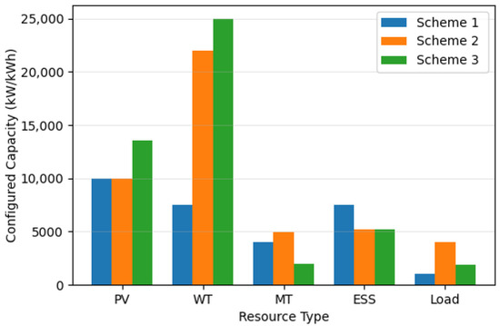
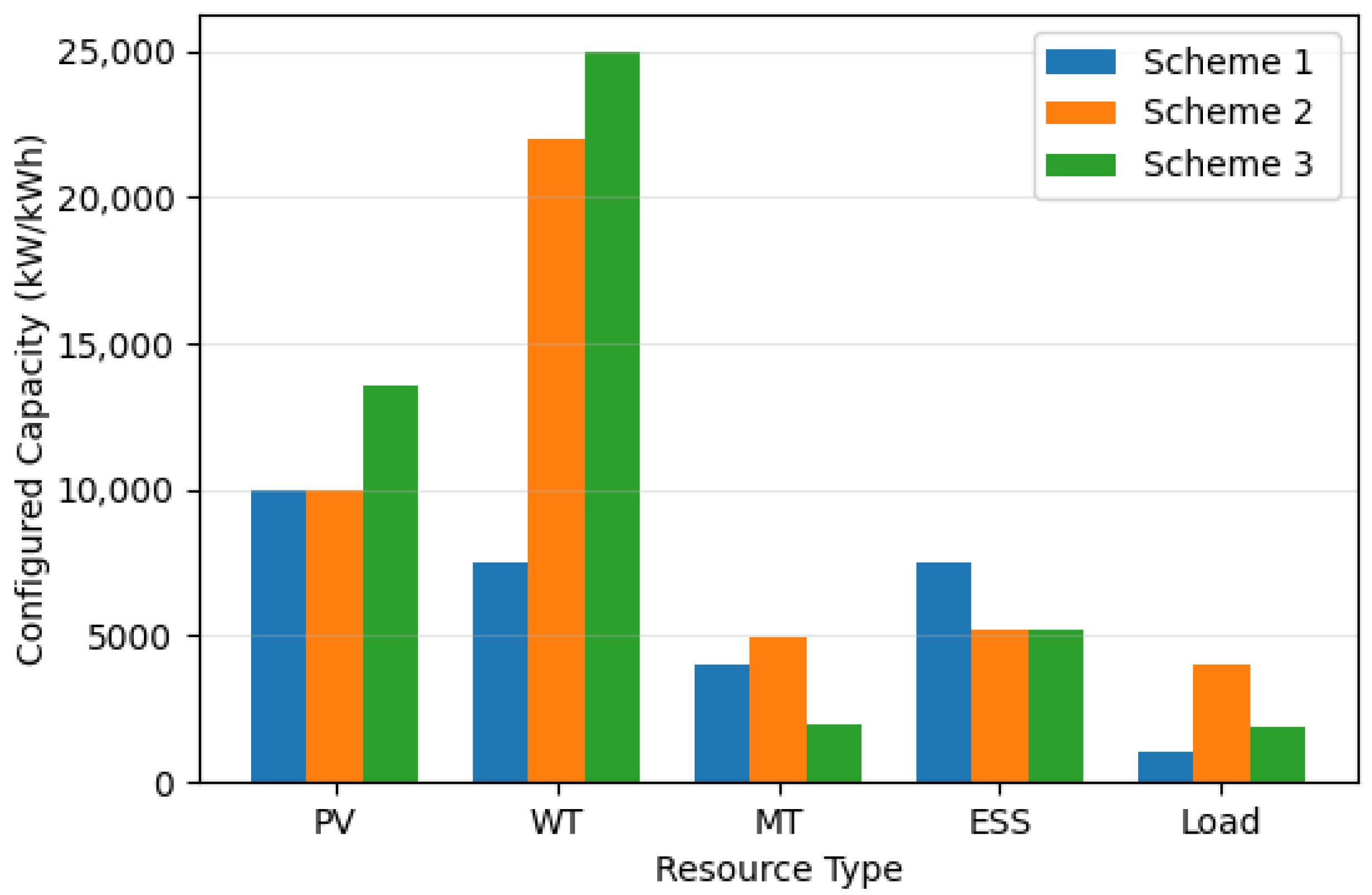
The DER capacity configuration results of each scheme are shown in Figure 1. From the optimization results, there are significant differences in capacity configurations and objective function values among the three coupling schemes.
Figure 1.
Comparison of VPP capacity configuration results for different schemes.
In Scheme 1, the capacities of PV and WT are relatively low, while the proportion of MT is relatively high, and the capacities of ESS and adjustable load are the smallest. This is because in the absence of inter-energy synergy, the system needs to rely on conventional power generation to ensure reliability, resulting in the highest objective function value. This confirms the theoretical conclusion that renewable energy accommodation is limited and the system comprehensive cost is relatively high under the independent planning mode.
Scheme 2 and Scheme 3 demonstrate the optimization value of the coupling mechanism: both have lower objective function values than Scheme 1, with significantly increased PV-WT capacities and reduced capacities of conventional units. This reflects that the coupling mechanism promotes renewable energy substitution for conventional power generation by strengthening the technical connections and economic interactions between energy devices.
The objective function of Scheme 3 is slightly higher than that of Scheme 2, while Scheme 3 has the highest PV-WT penetration rate and the lowest proportion of conventional units. This reflects that time-varying coupling, by dynamically adjusting the correlation intensity in different time periods, more accurately matches the intermittency of renewable energy and the temporal characteristics of loads. Theoretically, this verifies the core view that the dynamic coupling mechanism can better achieve the spatiotemporal balance between reliability and economy, providing a mechanism design basis for the optimal configuration of high-penetration renewable energy systems.
5.3.2. Power Output and Load Matching Characteristic Analysis
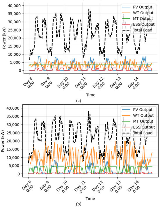
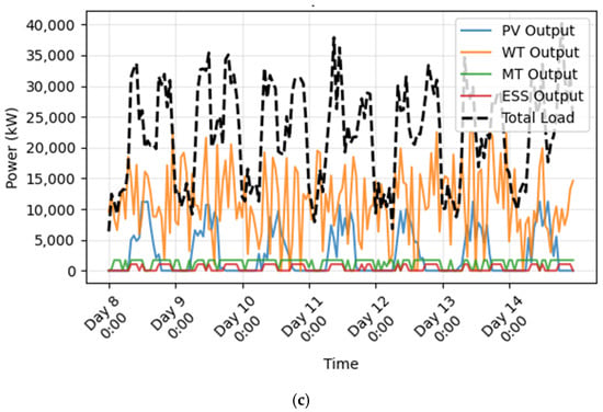
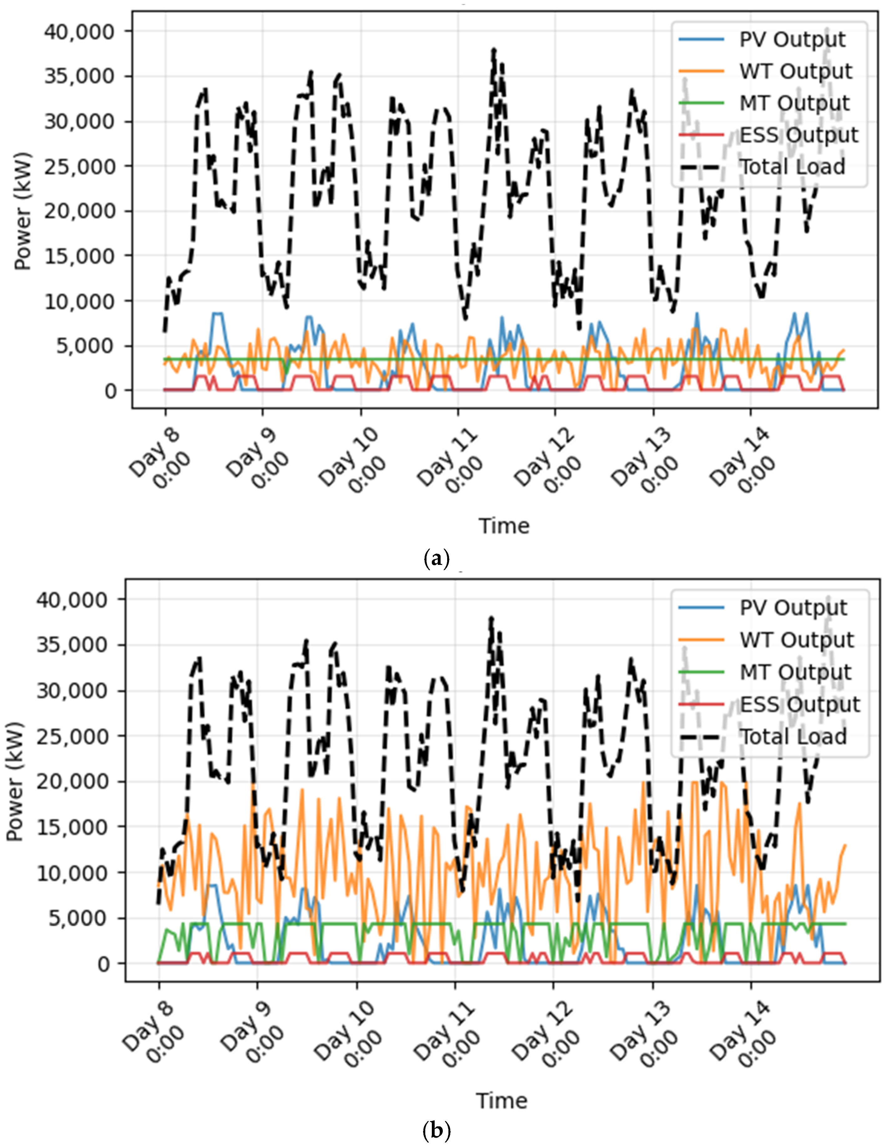
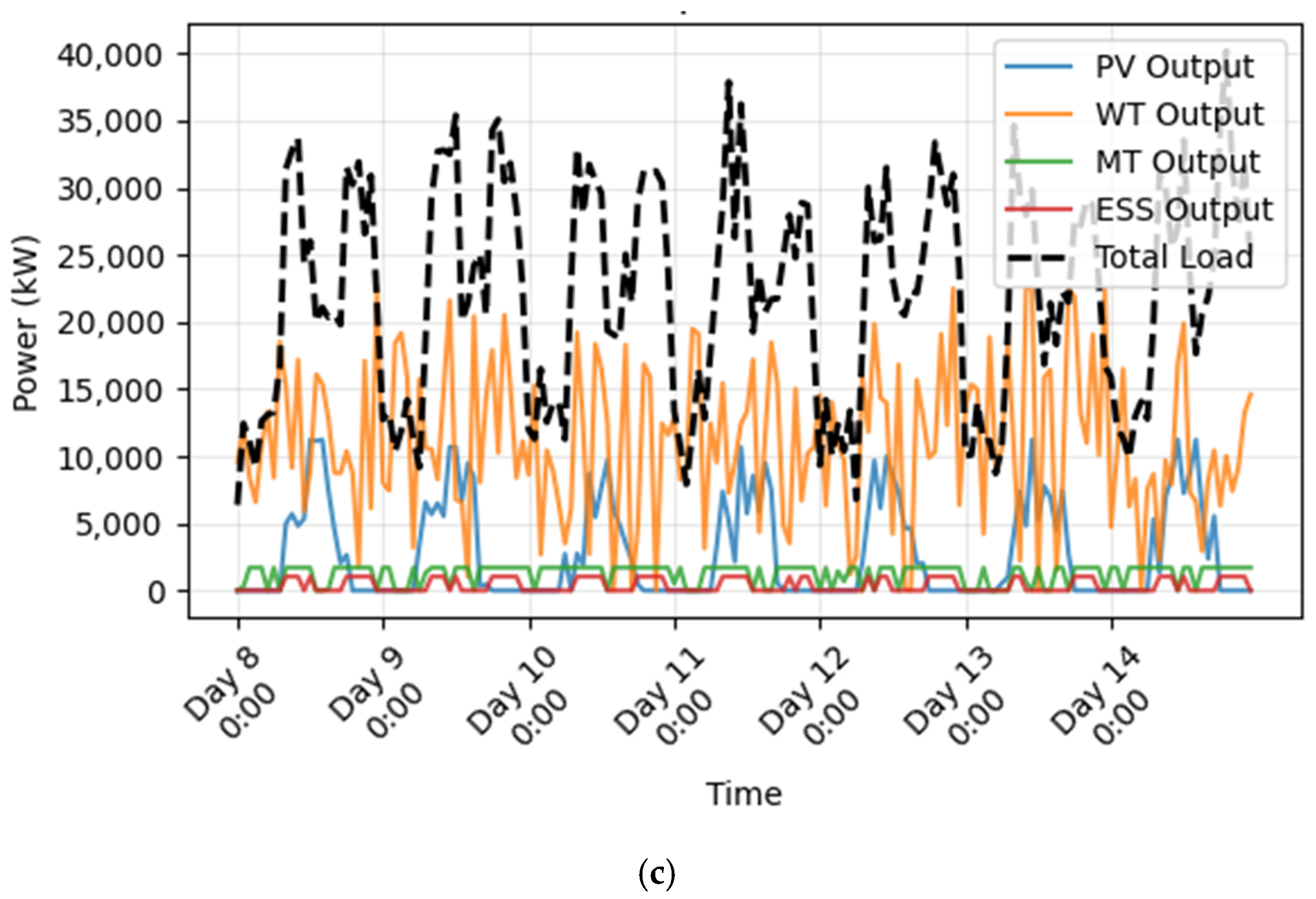
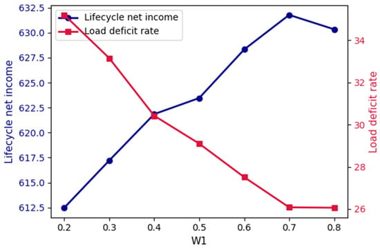
To intuitively demonstrate the dynamic adaptation between VPP output and load under different coupling schemes, Figure 2a–c present the power output curves of various resources and the total load curve for Scheme 1, Scheme 2, and Scheme 3 within a typical week, respectively.
Figure 2.
Comparison of power output curves of various resources and total load curve within a typical week. (a) Scheme 1. (b) Scheme 2. (c) Scheme 3.
It can be observed that in Scheme 1, due to the lack of consideration for coupling relationships between DERs, the volatility of PV and WT output is directly transmitted to the system’s total output, resulting in a significant deviation between the total output and the load curve. Compared with Scheme 1, Scheme 2 initially coordinates the output cooperation of various resources through fixed coupling coefficients: the output fluctuations of PV and WT are partially mitigated, and the charging–discharging response of the ESS becomes more regular. However, since the annual-average fixed coupling coefficients are adopted, it cannot adapt to the dynamic coupling requirements of different intraday periods. In scenarios with sudden load changes or severe fluctuations in PV-WT output (e.g., the period of sudden load surge on the afternoon of Day 13), phenomena such as delayed ESS regulation and lagged MT emergency startup still occur, leading to obvious short-term deviations between the total output and the load.
Scheme 3 benefits from dynamic coupling relationships captured by sliding time window correlation analysis and the coordinated configuration effect of the capacity correlation matrix. As a result, the output of various resources exhibits precise temporal coordination. Even in scenarios with sudden load fluctuations or sharp drops in PV-WT output caused by extreme weather conditions (e.g., the sudden load surge and WT output decline in the evening of Day 14), the system can quickly coordinate the output responses of the ESS, MT, and adjustable load through dynamic adjustment of time-varying coupling coefficients, ensuring that the total output closely aligns with the load curve. This fully demonstrates the core advantage of the time-varying power coupling mechanism in improving the system’s output flexibility and load adaptability.
5.3.3. Economic Indicator Comparison
The life-cycle is limited by the ESS’s life span, calculated over 10 years. Taking into account the benefits from power coupling, the composition and total volume comparison results are shown in Table 2.
Table 2.
Comparison of economic indicators (Unit: M CNY).
Table 2 shows that Scheme 3 has the lowest life-cycle net cost—negative, indicating the highest net income. The core reasons are as follows: On the one hand, the precise quantification of time-varying power coupling reduces the investment in redundant capacities; on the other hand, the capacity correlation matrix enables economic synergy between resources—for example, the capacity matching between PV and adjustable load—improves the self-consumption rate, and the rational configuration of MT capacity reduces fuel consumption, thereby optimizing the operating cost and market income.
5.3.4. Reliability and Resource Utilization Rate Comparison
Reliability is characterized by the load deficit rate, and the resource utilization level is characterized by the comprehensive resource utilization rate. The specific calculation adopts the weighted average of the actual operating duration and full-load operating duration of various resources; the comparison results are shown in Table 3.
Table 3.
Comparison of performance indicators.
From Table 3, it can be seen that the load deficit rate of Scheme 3 has decreased by 51.2% compared with Scheme 1 and by 24.6% compared with Scheme 2, and the power supply reliability has been improved; meanwhile, the comprehensive resource utilization rate has slightly increased. This indicates that the capacity configuration with time-varying power coupling enables the VPP to achieve precise resource dispatch in different periods (such as PV output peak periods, and periods when adjustable load and the ESS accommodate surplus electricity). Thus, while ensuring reliability, the resource utilization efficiency is also improved.
The simulation analysis of this study is based on the perfect forecast assumption using historical data, and the obtained reliability indicators such as the load deficit rate are derived under the condition of ignoring forecast errors. In practical applications, forecast errors will introduce uncertainty, which may lead to a certain degree of deterioration of reliability indicators. However, the time-varying coupling mechanism proposed in this study, by dynamically correlating resources, inherently possesses stronger robustness to mitigate fluctuations. Future research will incorporate a forecast error model to further verify the effectiveness of the proposed method in an uncertain environment.
5.3.5. Sensitivity and Robustness Verification
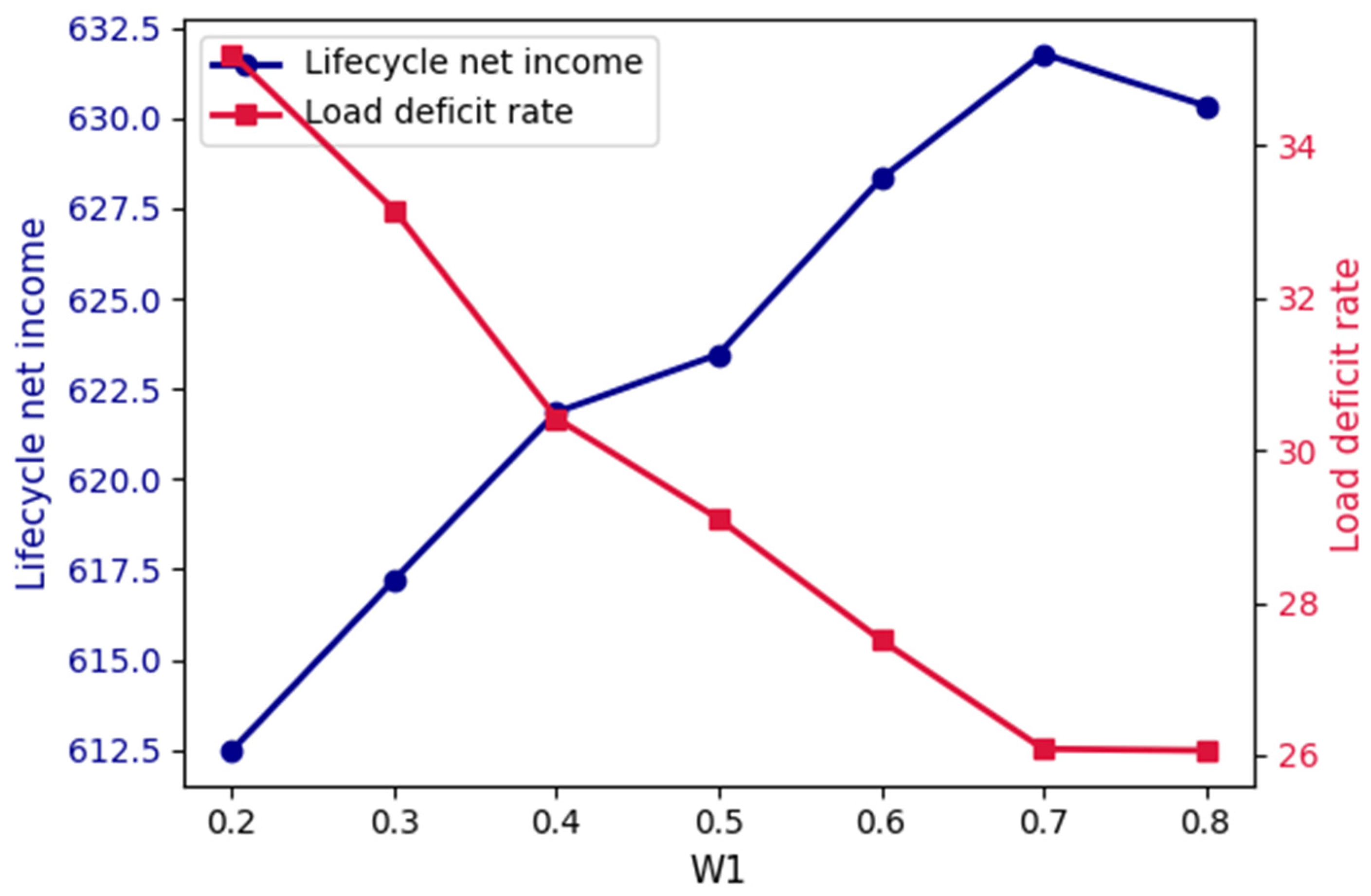
To verify the robustness of the proposed method and explore the sensitivity of the revenue weight in the objective function to the VPP’s life-cycle performance, a sensitivity analysis is conducted on the objective weight: the weight is adjusted to take values of 0.2, 0.3, 0.4, 0.5, 0.6, 0.7, and 0.8. The changes in the net income and load deficit rate of Scheme 3 under different weights are shown in Figure 3.
Figure 3.
Life-cycle net income and load deficit rate vs. .
From the perspective of economic performance, as increases from 0.2 to 0.7, the VPP’s life-cycle net income gradually rises from CNY 612.48 million to a peak of CNY 631.78 million; however, when , the net income slightly drops back to CNY 630.34 million. This trend stems from the fact that a higher strengthens revenue-oriented resource configuration, but when is too high, the law of diminishing marginal returns emerges, compressing the redundant optimization space for resource synergy, resulting in the net income growth showing a pattern of continuous decline followed by a slight rebound.
From the perspective of power supply reliability, the load deficit rate also shows a trend of continuous decline followed by a slight rebound as increases. When , the deficit rate reaches 35.2%; when , it drops to the minimum of 26.08%; when , it rebounds to 26.06%. The core logic is that a higher drives resource configuration to tilt toward a balance between revenue and reliability, and increased power supply redundancy reduces the deficit rate; however, when is too high, the revenue orientation squeezes the marginal optimization space of power supply redundancy, leading to a slight rebound in the deficit rate.
In summary, when is in the range of 0.6–0.7, the VPP’s life-cycle net income and power supply reliability achieve a relatively optimal synergistic balance. This range can be used as the recommended tuning range for the objective function weight parameter, verifying the significant regulatory effect of the weight parameter on VPP performance and providing a quantitative basis for parameter adaptation in practical configurations. In addition, regardless of parameter adjustments, the life-cycle net cost and load deficit rate remain lower than those of Scheme 1 and Scheme 2, indicating that the proposed method can achieve a balance between economy and reliability under different objective orientations.
In addition, to verify the sensitivity of the disturbance step (used in the numerical calculation of the economic synergy term in this paper’s capacity collaborative configuration model) and evaluate the stability of the final configuration scheme, this section conducts a sensitivity analysis on this parameter. The disturbance step is set as a percentage of the system rated capacity, with values of 1%, 2%, 5%, and 10%, respectively, and the proposed model is re-solved based on these settings. Among them, corresponds to the baseline result of Scheme 3 (time-varying power coupling scheme) in the main text. The capacity configuration and performance indicators under different disturbance step sizes are shown in Table 4.
Table 4.
Capacity configuration and performance indicators under different disturbance step sizes.
From the analysis of Table 4, when the disturbance step varies within the range of 1% to 10%, the fluctuation range of the configuration capacity of various resources is less than 2%. For example, the PV capacity fluctuates between 12.75 MW and 12.95 MW, the energy storage capacity fluctuates between 5.12 MWh and 5.20 MWh, and the adjustable load capacity fluctuates between 1.85 MW and 1.88 MW. The life-cycle net cost of the system and the load deficit rate change minimally: the maximum fluctuation of the net cost does not exceed 0.005%, and the maximum fluctuation of the load deficit rate does not exceed 0.04%.
Thus, the results indicate that the capacity collaborative configuration model constructed in this paper, as well as the calculation method of its economic synergy term, is insensitive to the value of the key parameter . Under different values, the optimized capacity configuration scheme and the final performance indicators remain highly stable, which verifies the strong robustness of the model and the reliability of the finally recommended configuration scheme (). This also provides a basis for selecting of the system rated capacity as the disturbance step in practical engineering applications.
5.3.6. Applicability Discussion of the Model in Networked VPP Scenarios
The simulation scenario of this paper is based on a single-bus VPP, and the effectiveness of the time-varying coupling mechanism and capacity collaborative allocation method is mainly verified. If the model is applied to multi-node networked VPPs, extensions are required in the following aspects: First, the constraint conditions need to add power flow equations, line capacity, and voltage upper/lower bound constraints; second, the capacity correlation matrix needs to introduce spatial correlation based on node impedance or power transfer distribution factors; third, the solution algorithm needs to address the non-convexity and scalability issues caused by these adjustments.
For residential VPPs, the internal DERs (e.g., residential PV, small-scale energy storage, adjustable household appliances) have smaller scales, larger quantities, and strong behavioral randomness. The method in this paper is still applicable in principle, but two adaptations are needed at the implementation level: first, the calculation of time-varying coupling coefficients may require shorter time windows to capture high-frequency fluctuations in users’ energy consumption; second, the capacity correlation matrix needs to place more emphasis on economic synergy terms to reflect residential users’ price sensitivity and response uncertainty.
In addition, the simulation analysis of this paper is based on fixed time-of-use electricity prices and ancillary service pricing mechanisms. In practical applications, the market structure of the VPP (e.g., pure spot market, bilateral contract market, or diverse market including capacity markets) and electricity price fluctuation characteristics (e.g., variance and peak-valley difference in real-time electricity prices) will also have a significant impact on its capacity allocation results. Different market mechanisms will change the revenue models and risk characteristics of DERs, thereby affecting the economic synergy terms in the capacity correlation matrix.
Preliminary analysis shows that in real-time markets with more volatile electricity prices, the time-varying power coupling mechanism can more sensitively capture the dynamic correlation between price signals and resource output, thus tending to allocate more flexible energy storage capacities and adjustable load capacities to enhance arbitrage capability and risk resilience. Future research can further construct extended models embedded with market clearing or electricity price stochastic processes to quantitatively evaluate the robustness of VPP capacity allocation strategies under market environment uncertainty. Furthermore, in terms of algorithm development, comparative verification with global optimization algorithms will be conducted to enhance the theoretical rigor and guarantee of global optimality in the model solution.
6. Conclusions
This paper proposes a coordinated capacity configuration method for VPP distributed resources considering time-varying power coupling. The main conclusions are as follows:
- By deriving the basic model of coupling coefficients based on Lagrange multipliers and integrating it with the STWCA, this approach establishes a calculation method for time-varying coupling coefficients that can accurately capture the intraday dynamic evolution of coupling relationships between DERs, providing refined, time-sequential coupling constraint support for capacity configuration. This method not only avoids capacity redundancy resulting from ignored resource synergy in independent configuration modes but also overcomes the configuration deviation caused by fixed coupling coefficients, which cannot adapt to dynamic scenario changes. Thus, it achieves precise dynamic matching of distributed resources across different operational periods.
- The capacity correlation matrix, integrating technical and economic dimensions, establishes an effective mapping from “dynamic power interaction at the operation layer” to “capacity configuration constraints at the planning layer” through the quantitative combination of the technical capacity correlation term and the economic synergy term. Specifically, the technical capacity correlation term reflects the cumulative impact of power interactions between resources on long-term capacity demands via the time-dimensional integral average of power coupling; the economic synergy term quantifies the marginal effect of the cost function to characterize the cross-impact of synergistic changes in resource capacities on the system’s total cost. Ultimately, this clarifies the capacity interdependence intensity and synergistic adjustment ratio between various resources, providing dual guarantees for the technical feasibility and economic rationality of capacity configuration.
- Case simulation results verify the superiority of the proposed method: compared with the traditional method (which ignores power coupling) and the configuration method (which uses fixed coupling coefficients), this method can significantly reduce the VPP’s life-cycle net cost and effectively control investment redundancy and operation losses. Meanwhile, the load deficit rate is reduced by 51.2% (vs. the traditional method) and 24.6% (vs. the fixed coupling method), while the comprehensive utilization rate of distributed resources is improved simultaneously. This successfully resolves the core contradiction between “wind/solar curtailment” and “insufficient power supply” in high-penetration renewable energy integration scenarios, achieving synergistic optimization of economy and reliability.
The coordinated capacity configuration method proposed in this study verifies the effectiveness of the time-varying power coupling mechanism in the single-bus VPP scenario, laying a foundation for understanding the dynamic collaboration of distributed resources. To promote the extension of this method to practical engineering applications, future research will focus on constructing a multi-node VPP capacity allocation model that integrates network power flow constraints, systematically characterizing the spatial-dimensional coupling and cross-regional mutual support mechanisms, and introducing a dynamic adjustment mechanism of market policies. This will enhance the model’s adaptability to complex power grid environments and market conditions, thereby supporting the scientific planning and efficient operation of virtual power plants in the new power system.
Author Contributions
Conceptualization, L.Y.; methodology, L.Y. and L.X.; software, K.Z. and J.S.; validation, L.Y.; investigation, L.Y. and J.S.; data curation and resources, L.Y. and L.S. All authors have read and agreed to the published version of the manuscript.
Funding
This research was funded by the Research Funds of Sanjiang University, “Research on Key Optimization Strategies of Integrated Virtual Power Plants for Multi-Market Collaborative Trading, grant number 2025SJKY002”.
Data Availability Statement
The original contributions presented in this study are included in the article. Further inquiries can be directed to the corresponding author.
Conflicts of Interest
Author Lingxiang Shen was employed by the company HELLA (Nanjing) Electronics Co., Ltd. The remaining authors declare that the research was conducted in the absence of any commercial or financial relationships that could be construed as a potential conflict of interest.
Abbreviations
The following abbreviations are used in this manuscript:
| VPP | Virtual Power Plant |
| DER | Distributed Energy Resource |
| PV | Photovoltaic |
| WT | Wind Turbine |
| MT | Micro Turbine |
| ESS | Energy Storage System |
| L | Adjustable Load |
| STWCA | Sliding Time Window Correlation Analysis |
| SLSQP | Sequential Least Squares Programming |
| SOC | State of Charge |
Appendix A
Table A1.
Main symbols.
References
- dos Santos, J.A.; Binotto, J.M.; Piardi, A.B.; Pavani, A.P.G.; Vieira Junior, J.C.M.; Ramos, R.A. Short-Term Voltage Stability Analysis Considering the Mandatory Disconnection of Distributed Energy Resources. J. Control Autom. Electr. Syst. 2025, 36, 1180–1195. [Google Scholar]
- Liu, X.; Gu, X.; Guo, J.; Yang, X.; Chen, T. Dynamic adjustment method for the configuration of distributed energy resources in virtual power plants. Int. J. Electr. Power Energy Syst. 2025, 173, 111352. [Google Scholar] [CrossRef] [Scilit]
- Borisoot, K.; Liemthong, R.; Srithapon, C.; Chatthaworn, R. Optimal Energy Management for Virtual Power Plant Considering Operation and Degradation Costs of Energy Storage System and Generators. Energies 2023, 16, 2862. [Google Scholar] [CrossRef] [Scilit]
- Ullah, Z.; Hassanin, H.; Cugley, J.; Alawi, M.A. Planning, Operation, and Design of Market-Based Virtual Power Plant Considering Uncertainty. Energies 2022, 15, 7290. [Google Scholar] [CrossRef] [Scilit]
- Ropuszynska-Surma, E.; Weglarz, M. The Methods of Assessing the Efficiency of a Virtual Power Plant-Case Study. Energies 2024, 17, 174. [Google Scholar] [CrossRef] [Scilit]
- Huang, J.; Li, H.; Zhang, Z. Review of Virtual Power Plant Response Capability Assessment and Optimization Dispatch. Technologies 2025, 13, 216. [Google Scholar] [CrossRef] [Scilit]
- Li, C.; Tian, S.; Dai, J.; Peng, S.; Zhu, S.; Jiang, Y.; Guo, R. Credible capacity forming of a VPP with wind, solar, and storage resources. Energy Convers. Econ. 2025, 6, 256–267. [Google Scholar] [CrossRef] [Scilit]
- Zhang, R.F.; Hredzak, B. Distributed Dynamic Clustering Algorithm for Formation of Heterogeneous Virtual Power Plants Based on Power Requirements. IEEE Trans. Smart Grid 2021, 12, 192–204. [Google Scholar] [CrossRef] [Scilit]
- Zuo, J.; Xu, C.; Wang, W.; Huang, Y.; Xu, T.; Ji, Y. Different Types of Energy Storage Capacity Optimization Allocation Strategies in Virtual Power Plant Considering Dynamic TOU And Conditional Value at Risk. In Proceedings of the 7th Asia Energy and Electrical Engineering Symposium (AEEES 2025), Chengdu, China, 28–31 March 2025; pp. 1551–1555. [Google Scholar]
- Wang, C.L.; Wang, H.; Ji, X.; Xu, H.; Yang, C.D.; Meng, X.P. Hybrid energy storage capacity configuration strategy for virtual power plants based on variable-ratio natural gas-hydrogen blending. Int. J. Hydrogen Energy 2024, 58, 433–445. [Google Scholar] [CrossRef] [Scilit]
- Bai, X.; Fan, Y.; Liu, Y.; Song, Y. Wind power storage virtual power plant considering reliability and flexibility tiered capacity configuration. Power Syst. Prot. Control 2022, 50, 11–24. [Google Scholar]
- Wang, S.; Jia, R.; Shi, X.; Luo, C.; An, Y.; Huang, Q.; Guo, P.; Wang, X.; Lei, X. Research on Capacity Allocation Optimization of Commercial Virtual Power Plant (CVPP). Energies 2022, 15, 1303. [Google Scholar] [CrossRef] [Scilit]
- Liu, Y.; Fan, Y.; Hao, J.; Bai, X.; Song, Y. Capacity configuration and optimal scheduling of a wind-photovoltaic-hydrogen-thermal virtual power plant based on a wide range power adaptation strategy for an alkaline electrolyzer. Power Syst. Prot. Control 2022, 50, 48–60. [Google Scholar]
- Yu, S.; Dong, X.; Lu, T.; Wu, Y.; Wang, C.; Wang, Y. Emergency control scheme for high distributed energy penetrated systems considering electro-thermal coupling effect. Sustain. Energy Grids Netw. 2025, 43, 101885. [Google Scholar] [CrossRef] [Scilit]
- Zhang, Y.; Yan, X. Coupling Analysis and Decoupling Control of Microgrid Power. Power Syst. Technol. 2016, 40, 812–818. [Google Scholar]
- Gao, H.J.; Chen, Q.Z.; He, S.J.; Tang, Z.Y.; Li, H.B.; Liu, J.Y. Electricity-carbon coupling retail package optimization considering low-carbon benefits of distributed renewable energy. J. Clean. Prod. 2024, 449, 141598. [Google Scholar] [CrossRef] [Scilit]
- Liang, Z.; Wang, L.; Li, J. Nash Equilibrium Based Optimal Control Method for Hydrogen Production System with Photovoltaic-Storage Coupling. Autom. Electr. Power Syst. 2025, 49, 125–134. [Google Scholar]
- Jiang, H.B.; Huang, H.F.; Zhang, Y.L.; Xu, X.W.; Zhao, Y.J. The Impact of Installation Angle on the Wind Load of Solar Photovoltaic Panels. Processes 2024, 12, 1077. [Google Scholar] [CrossRef] [Scilit]
- Li, X.Y.; Wang, Z.H. Optimization of Photovoltaic-Wind Power Coupling System for Virtual Power Plant. Energy Convers. Manag. 2023, 285, 117982. [Google Scholar]
- Zou, Q. Distribution System Reliability and Security Evaluation based on Matrix Analytical Calculation. Master’s Thesis, Tianjin University, Tianjin, China, 2021. [Google Scholar]
- Pfeiffer, K.; Kheddar, A. Sequential hierarchical least-squares programming for prioritized non-linear optimal control. Optim. Methods Softw. 2024, 39, 1104–1142. [Google Scholar] [CrossRef] [Scilit]
- XIHE Energy Meteorological Big Data Platform [EB/OL]. Available online: https://xihe-energy.com/ (accessed on 10 August 2025).
- State Grid Jibei Electric Power Co., Ltd. Jibei Power Trading Platform [EB/OL]. Available online: https://pmos.jibei.sgcc.com.cn/ (accessed on 10 August 2025).

Disclaimer/Publisher’s Note: The statements, opinions and data contained in all publications are solely those of the individual author(s) and contributor(s) and not of MDPI and/or the editor(s). MDPI and/or the editor(s) disclaim responsibility for any injury to people or property resulting from any ideas, methods, instructions or products referred to in the content. |
© 2026 by the authors. Licensee MDPI, Basel, Switzerland. This article is an open access article distributed under the terms and conditions of the Creative Commons Attribution (CC BY) license.