


Abstract
Thermal observations may be consistent with several adjacent components of power equipment. CSET-3D associates them with a component-labeled exterior surface reconstructed from an RGB stereo pair. The thermal transport plan uses projection and visibility costs and an unresolved destination. Admission and support rules determine which observations contribute to component descriptors. A separate acoustic plan provides exploratory direction-to-surface association. All quantitative results are based on a computational reference scene model with reference-derived disparity, component masks, and 3D–2D correspondences. The learned stereo, segmentation, and XoFTR front ends are outside the quantitative evaluation. The Foshan field demonstration is qualitative. The primary evaluation comprises 500 cases. In the 100 nominal cases, CSET-3D has lower integrated thermal attribution error over common attainable coverage than the residual-ranked nearest-hard and point-cloud comparators, with lower default correct yield and retention. Acoustic correct yield is lower than for both comparators. The findings characterize the trade-off between thermal attribution error and evidence retention on the modeled exterior surface.
1. Introduction
Component-level thermal inspection requires associating image responses with their corresponding regions on the equipment surface. Closely spaced bushings, terminals, radiators, and enclosures make attribution sensitive to geometry and component boundaries. CSET-3D uses RGB stereo to establish metric positions and component identities on the visible exterior. This surface also supplies candidates for exploratory acoustic association. Here, 3D denotes metric coordinates on the stereo-visible exterior in a single view, an effectively 2.5D representation.
Spatial proximity alone does not establish that observations originate from the same component. Components at different depths may project onto adjacent image pixels, allowing small calibration errors to shift a projected thermal observation across a component boundary. Moreover, a surface visible in the stereo images may be occluded in the thermal view. Acoustic observations introduce additional ambiguity: a single estimated direction of arrival may intersect multiple candidate surfaces, while reflections may produce spurious directions. Recent 3D segmentation studies distinguish semantic categories from instance identities [1,2,3], while multimodal acoustic localization methods use visual and geometric cues to reduce directional ambiguity [4,5,6,7]. These considerations motivate an association framework that accounts for component identity, depth, and visibility.
Stereo reconstruction provides estimates of equipment surface geometry [8,9,10,11,12]. Cross-spectral registration establishes correspondences between visible-light and thermal infrared imagery [13,14,15,16,17,18], whereas acoustic localization estimates source directions from microphone-array measurements, potentially supplemented by visual or multiview information [4,5,6,7,19,20,21]. Reliability-aware fusion accounts for variations in observation quality and availability [22,23,24]. Collectively, these methods provide essential information about geometry, cross-modal correspondence, source direction, and measurement reliability. However, component-level attribution remains challenging when multiple candidate surfaces are consistent with the available evidence.
The main contribution of CSET-3D is component-constrained thermal-to-surface association. The method applies established entropic unbalanced transport to a component-labeled stereo surface. Projection, visibility, and component-boundary costs constrain thermal assignments, and an unresolved destination accommodates observations with insufficient surface compatibility. Source admission and area-weighted aggregation produce component-level thermal descriptors. The exploratory acoustic branch associates single-array directions with the same exterior surface. The thermal and acoustic transport plans are optimized independently. Equation (16) assembles the reconstructed channels and a local co-occurrence term into an output descriptor after transport.
Reliable thermal–acoustic correspondence could help resolve ambiguous assignments if both observations are known to arise from the same source or component. Enforcing such correspondence when the observations have different physical causes could instead introduce errors. The present objective does not model that source correspondence. The shared-target-prior control in Table S7 tests one coupling alternative without introducing same-source identities. Local co-occurrence is retained as a descriptor rather than treated as evidence of a common fault.
2. Related Work
2.1. Metric Geometry and Component-Level 3D Surfaces
Stereo estimation supplies metric geometry, while segmentation supplies component identity. Disparity from semiglobal matching [12], recurrent stereo networks [10,11], or FoundationStereo models [8,9] supports depth recovery. D-FINE [25] performs object detection; the local segmentation extension used in the component interface additionally generates masks. A depth error displaces a surface node, whereas a mask error can assign it to the wrong component. The controlled evaluation in Section 4 uses perturbed reference disparity and reference component maps and therefore does not measure the performance of these learned front ends.
Semantic segmentation labels the category of each 3D point, while instance segmentation distinguishes individual objects; panoptic segmentation performs both tasks. Point Transformer V3 extracts point-cloud features [1], OneFormer3D handles semantic, instance, and panoptic segmentation within one model [2], and Mask4Former links instances across LiDAR sequences [3]. In CSET-3D, masks obtained from images partition the reconstructed surface for thermal and acoustic attribution. These component identities apply within individual frames, and the model does not perform temporal panoptic tracking.
2.2. 3D Association of Thermal and Acoustic Evidence
Reliable thermal mapping requires correspondences, pose estimates, and visibility information. Sparse feature detection and matching are provided by SuperPoint and LightGlue [13,14]; RIFT and XoFTR address appearance differences across spectra [15,16]. Correspondences support geometric alignment through RANSAC and PnP [26,27]. Non-planar registration [17] and thermal point-cloud reconstruction [18] further accommodate spatial variation in visible–thermal geometry. CSET-3D carries this association onto surface candidates labeled by component. Its assignment costs include reprojection, depth, and boundary terms, while observations without reliable assignments remain at an unresolved destination.
Earlier RGB–thermal studies of power equipment examined feature interaction and image-based recognition [28]. Our evaluation instead concerns the attribution of thermal and acoustic observations to metric component surfaces. In acoustic processing, GCC-PHAT estimates interchannel delays [19], and SRP-PHAT aggregates pairwise responses across candidate directions [20,21]. LOCATA benchmarks localization in moving and reverberant scenes [4]. AcousticFusion, Sound3DVDet, and SoundLoc3D use visual, multiview, or RGB-D observations [5,6,7]. Here, directions from one array are compared with the reconstructed exterior surfaces. A direction may remain compatible with several components because the array does not independently measure range.
2.3. Quality-Aware Fusion and Equipment Multiphysics Perception
Reliability-aware fusion and missing-modality methods address variations in observation quality and availability [22,23]. Selective prediction evaluates error together with the fraction of retained observations [24]. Entropic optimal transport and generalized scaling for unbalanced transport provide allocation tools [29,30]. An unmatched destination, often called a dustbin or sink, also appears in learned matching such as SuperGlue [31]. CSET-3D applies these tools to component-labeled exterior surfaces, with projection and visibility costs for thermal observations and direction-to-surface compatibility for acoustic evidence. Post-allocation admission and support rules determine contributions to component descriptors. Point-cloud segmentation [1,2,3], thermal mapping [17,18] and equipment-image registration [32] provide related geometry and correspondence operations. Section 4.3 evaluates the attribution step against a calibrated point-cloud comparator using the same surface and component masks.
3. Component-Constrained Evidence Transport in CSET-3D
3.1. CSET-3D Framework
The inputs are a rectified left–right RGB image pair, a thermal frame, and multichannel array waveforms referenced to a common observation time. Stereo geometry and component masks supply the shared exterior surface. Equation (1) collects the sensor calibration and timing metadata required to express the observations in that frame. The output records component geometry, modality response, heuristic reliability, and the represented area supported by each modality.
The calibration set Θ in Equation (1) comprises the intrinsic and distortion models for all three cameras, the stereo baseline, and the rigid transformations connecting the thermal and array frames to the stereo frame. It also contains microphone coordinates, sampling rate, steering directions, sound speed, and the time offsets of thermal and acoustic measurements relative to the RGB observation. These quantities establish shared spatial and temporal references. Disparity, component identities, and cross-spectral correspondences then pass from the front ends to the allocation module.
Source admission determines whether an optimized observation assignment can contribute to reconstruction. Node support requires sufficient admitted mass and positive modality availability at a surface node. These deterministic rules are applied after transport. The sink is a separate optimization destination; post-processing leaves its assigned mass unchanged. The output retains visual appearance, thermal image response, acoustic directional response and reliability as separate channels.
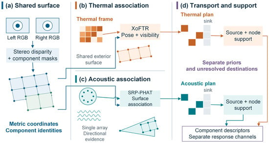
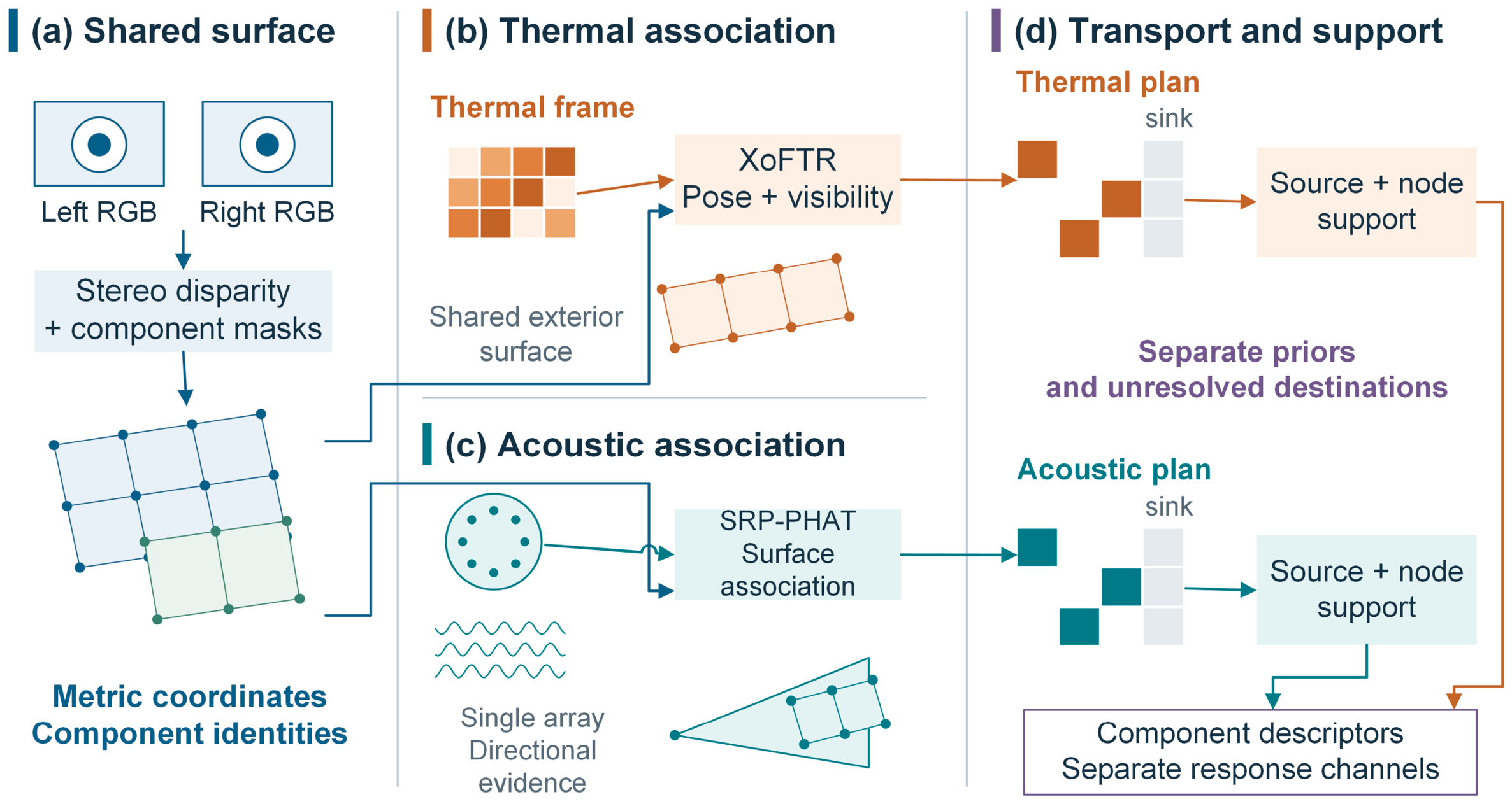
The architecture in Figure 1 comprises four linked stages. Stereo disparity and component masks form the common metric component surface in panel (a). In the thermal branch, panel (b), RGB–thermal matches and stereo depth support relative-pose refinement and visibility assessment. The acoustic branch in panel (c) extracts directions from array waveforms and selects candidate surfaces. Panel (d) solves a separate unbalanced transport plan for each modality, checks source and node support, and aggregates the accepted responses for each component.
Figure 1.
CSET-3D framework: (a) shared metric component surface; (b) thermal mapping; (c) acoustic mapping; (d) separate transport plans and component-state aggregation. Surface geometry is schematic.
The two branches share surface geometry and component identities, but their observations need not represent the same physical cause. The model inputs contain no verified thermal–acoustic source correspondences on which to impose joint assignments. Separate plans therefore express the chosen task: associate each observation with the surface while retaining its modality and unresolved evidence. Equation (11) uses modality-specific costs, target priors, and sinks, with no coupling term. This makes the stated objective separable; it neither proves statistical independence nor establishes that separate transport outperforms a joint model. Reliable cross-modal correspondences could motivate a different, coupled objective. A controlled shared-prior comparison in Section 4.6 and Table S7 tests one explicit coupling alternative without assuming cross-modal source identities.
3.2. Stereo Geometry and Component-Level 3D Surface Encoding
Fast-FoundationStereo [8] estimates disparity from the rectified RGB pair. Equation (2) converts valid positive disparity into metric depth using the calibrated focal length and stereo baseline. A heuristic stereo-quality weight combines the photometric warp residual and local disparity variation. It downweights poor image agreement and abrupt disparity changes; it is not a calibrated depth-error variance. Table A1 lists the numerical scales and validity thresholds.
In this expression, di denotes disparity in pixels predicted by Fast-FoundationStereo at rectified pixel (ui,vi); fx denotes the horizontal focal length in pixels, and B the baseline in meters. The recovered quantities Zi = fxB/di and xi therefore have metric units. Valid nodes must have finite correspondences and satisfy di > 10−6px. Stereo support is given by , with a validity indicator that vanishes outside the accepted stereo domain. The same weight enters surface-capacity and reliability calculations. Depth recovery assumes rectified intrinsics with zero skew. Appendix A lists the disparity floor.
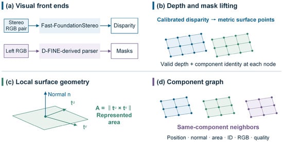
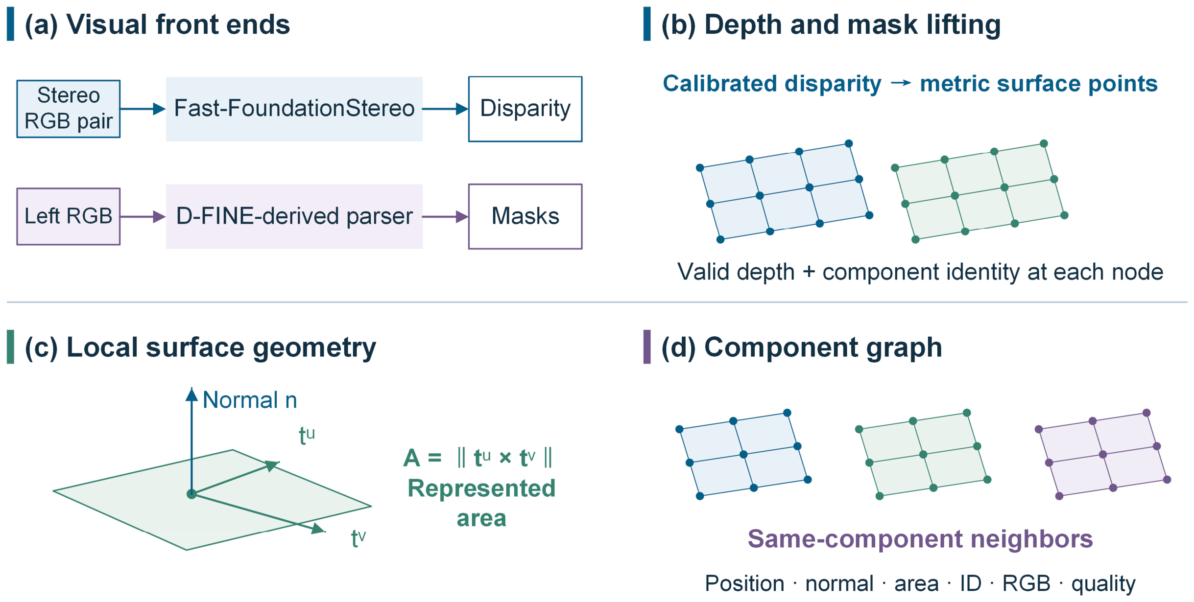
The component parser uses a D-FINE-derived segmentation model with an HGNetv2-S backbone, DFINESegTransformer, and SegPostProcessor. Resized mask logits are thresholded, low-score and small masks are removed, and the higher-scoring mask owns an overlapping pixel. Mask indices define component identities within the frame. Appendix A records the interface resolution and acceptance settings. Figure 2 links the visual inputs, joint depth-mask back-projection, local surface geometry, and same-component graph.
Figure 2.
Method schematic for surface construction: (a) Visual front ends and their outputs; (b) Joint depth and mask back-projection; (c) Local tangents, surface normal, and represented area; (d) Same-component graph and node attributes. The front-end inputs used in the evaluation are specified in Section 4.1.
A surface node is specified in Equation (3), and the graph links valid adjacent nodes belonging to the same component. Class labels, boxes, instance scores, and mask logits come from the parser; ci is taken from the accepted mask with the highest score. Pixels lacking a known component identity are excluded. Two grid tangents within the component determine . Orienting their normalized cross-product toward the stereo camera gives ni, and stores normalized RGB values.
Two image-grid tangents within the same component define the local normal and represented area. The horizontal tangent uses the right neighbor, with the left as fallback; the vertical tangent uses the lower neighbor, with the upper as fallback. A node is removed if a valid tangent is unavailable or its cross-product area fails the area floor. The normal points toward the stereo camera. Four-neighbor graph edges also require matching component identities and sufficiently similar normals. The radius and area floor affect node retention; the normal threshold acts on graph edges. Their values and roles appear in Appendix A. Their separate effects are tested in Section 4.6 and Table S3. The tested settings characterize local geometric sensitivity.
3.3. Cross-Spectral Matching and Visibility-Constrained Thermal Mapping
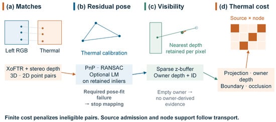
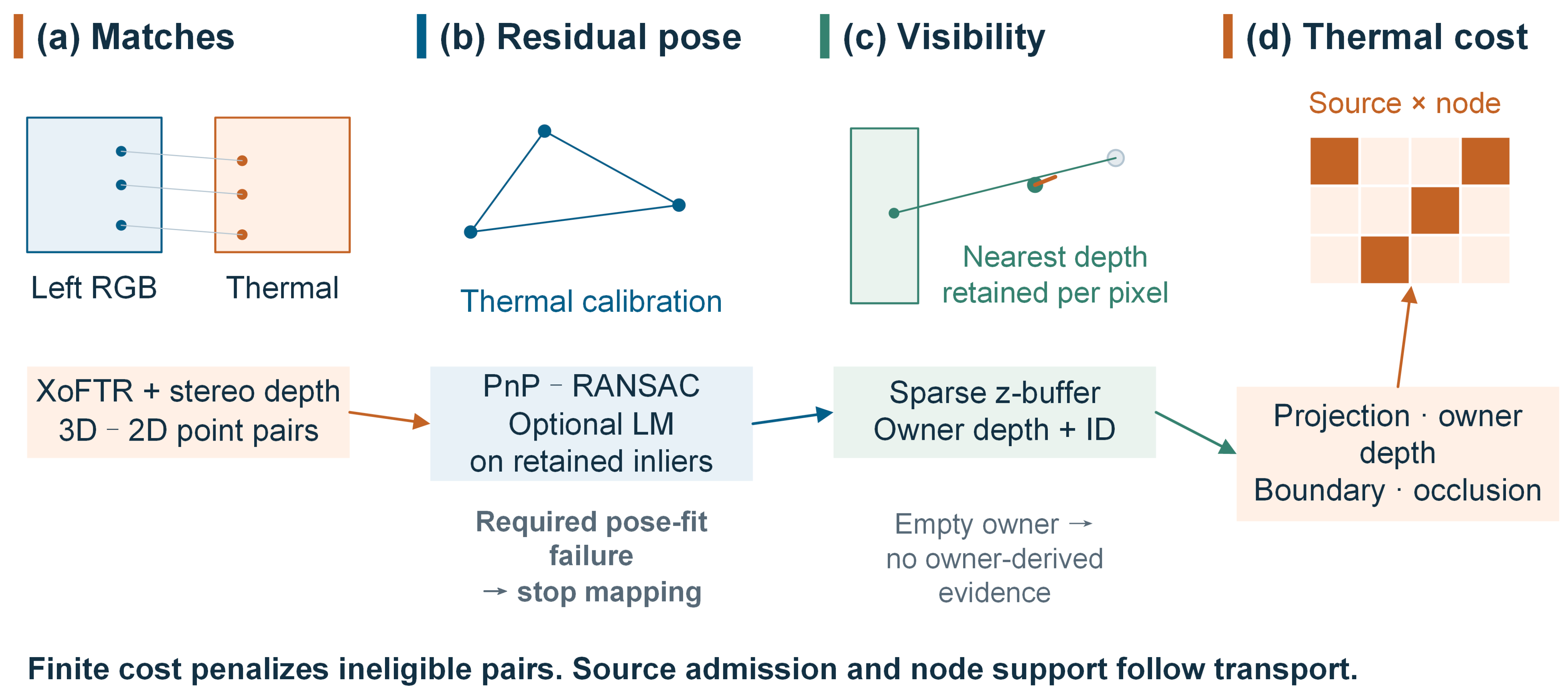
XoFTR [16] supplies RGB–thermal correspondences, and stereo depth maps the RGB locations to metric 3D points. PnP with RANSAC estimates the residual relative pose in Equation (4) [26,27]. Levenberg–Marquardt refinement, when available, uses the retained inliers. Projection includes thermal intrinsics and distortion. Failure of a required pose estimate terminates mapping. Figure 3 separates pose estimation, thermal-view visibility, and cost construction; Appendix A lists the implementation settings.
Figure 3.
Thermal association from cross-spectral correspondences to pose refinement, visibility, and modality-specific costs. A failed required pose estimate terminates mapping. An empty local owner does not supply depth or component evidence. Transport and source admission are separate stages.
Equation (4) pairs the homogeneous stereo point with its XoFTR correspondence in the thermal image. Thermal distortion is included in the projection . RANSAC forms the inlier set using the residual and minimum-inlier settings in Appendix A. Equation (5) then uses the refined pose. A failed required estimate terminates mapping.
A sparse z-buffer identifies the nearest reconstructed node at each thermal pixel in Equation (5). A local owner supplies depth and component information for a thermal sample, while a projection gate selects candidate nodes. An empty neighborhood has no owner. A surface missing from the stereo reconstruction is unavailable to this branch. Thermal values are image-response units: the numeric intensity or response scale supplied by the thermal input, without an assumed conversion to degrees Celsius.
After the rigid transformation, the projected location is and the third coordinate is . For each integer pixel inside the image, o(p) selects the nearest positive-depth node among those rounded to that pixel; for an empty pixel, the owner is −1. Thus, Equation (5) keeps only the z-buffer owners. For a thermal sample j, ι(j) denotes the nearest-depth owner in the local neighborhood specified in Appendix A. Its depth and component identity define the corresponding terms in Equation (9). Without a local owner, these terms contain no owner-derived evidence and cannot provide a thermal depth estimate.
Pose refinement reduces errors in the fitted correspondences, whereas visibility restricts assignment to reconstructed surfaces that can receive the observation. These operations address different sources of association error. Near component boundaries, even a small reprojection residual can accompany an incorrect assignment. We therefore combine image distance with depth consistency and boundary information in the thermal cost.
3.4. Acoustic Direction Encoding and Geometry-Constrained Surface Association
The acoustic front end removes each channel’s frame mean, computes windowed cross-spectra, and applies GCC-PHAT and SRP-PHAT over the retained frequency band. Peak contrast and pair quality determine candidate retention. Silence and an empty frequency band return no sources. Pair quality is derived from the GCC peak-to-RMS ratio, and grid quality from the band-limited cross-spectra. Their product controls source weighting and angular compatibility. The resulting directional spread is a compatibility parameter, not a calibrated confidence interval. Appendix A lists the spectral and peak-selection settings. Plane-wave steering assumes appropriate array geometry, channel timing, and far-field airborne propagation.
The cross-spectrum relates microphone channels m and within window h. PHAT normalization takes the form
Averaging across windows yields . Given microphone positions rm, sound speed cs, and steering direction d, the associated delay is . Equation (7) sums the phase-aligned responses across Np microphone pairs and Nf selected positive-frequency bins in .
The peak-selection settings are listed in Appendix A. Grid quality is obtained by clipping the mean magnitude of across the same pairs and bins. Its product with the clipped pair-quality score is . For accepted peaks, σθ,k = 6°/qpair sets the directional compatibility scale. The peak and quality thresholds also determine when the source set is empty.
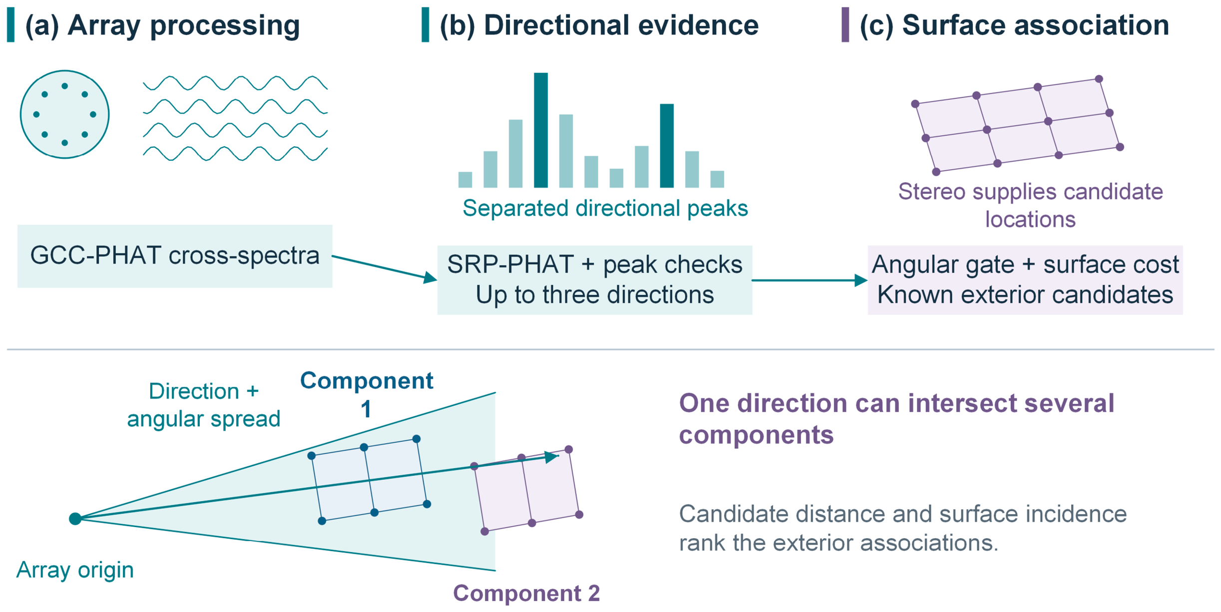
Equation (8) compares each retained direction with rays from the array to the known exterior surface. The angular cone restricts eligible nodes. Relative range and normal incidence order these candidates using the supplied geometry; they do not measure acoustic range. When a cone intersects several components, the transport plan ranks the competing surface assignments. This is an exploratory direction-to-surface association, not independent 3D source localization.
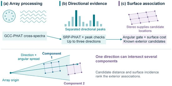
The ray to a surface point is ; it is normalized as only when its range is positive. Before computing the angle, the rotation RV←A is applied once to express the array direction in the stereo frame. Eligible nodes must satisfy θki ≤ max(20°,3σθ,k) and have positive acoustic visibility. Exterior-surface availability defaults to . Equation (8) defines both the angular cost and the angular residual after assignment without estimating acoustic range. Figure 4 traces this direction-to-surface association. Following contrast and quality checks, GCC-PHAT and SRP-PHAT supply up to three candidate directions, with pair quality determining the angular compatibility scale. Geometry and ambiguity between components constrain the costs before source admission. The resulting output records exterior-surface associations with accepted support.
Figure 4.
Acoustic directions and their association with candidate exterior surfaces. GCC-PHAT and SRP-PHAT provide directional evidence and heuristic quality. The surface geometry supplies candidate locations. A single array does not independently measure range, and multiple components may remain compatible with one direction.
The shared metric surface constrains acoustic directions to candidate components at different depths. Ambiguity remains where a direction is compatible with several surfaces. Direction error, exterior-surface association error, and component-attribution yield therefore quantify different aspects of acoustic performance.
3.5. Separate Evidence Transport and Component Descriptors
Module D constructs separate thermal and acoustic costs. The thermal cost in Equation (9) combines projection distance, local-owner depth consistency, component-boundary risk, and occlusion. The acoustic cost in Equation (10) combines angular compatibility, relative range and incidence, component ambiguity, and boundary risk. Appendix A records the cost scales and weights. Ineligible pairs receive a finite high cost. A finite cost is a soft numerical barrier and does not by itself guarantee zero transport; positive modality visibility is required later for supported reconstruction.
Using the eligibility indicator χ, we introduce the finite cost operator . Separate expressions define the thermal and acoustic costs:
The quantity measures projection distance between a source and a node and is distinct from the residual used to fit PnP. Eligibility requires a positive-depth node projected inside the image and a distance within the projection gate in Appendix A. When the local owner is known, ; the value is zero otherwise. The boundary term accounts for both mismatch with the known owner’s identity and the node’s boundary risk. Occlusion is indicated by one only if a known owner lies in front of the node by more than the occlusion tolerance in Appendix A.
Boundary risk βi decreases exponentially with grid distance from the component boundary on the scale specified in Appendix A. Component ambiguity αk is zero when no more than one component is eligible; with multiple eligible components, it is one minus the reciprocal of their count. The range-incidence term is , where subtracts the scene-minimum range and divides by the difference between the 95th percentile and minimum range. Its denominator has a floor of 10−12 m, and the result is clipped to [0,1]; . These dimensionless quantities rank exterior candidates without adding depth information.
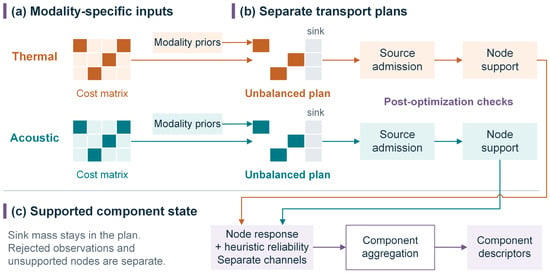
Equation (11) combines spatial cost, entropic regularization, and penalties on departures from the source and target priors. It is applied independently to the thermal and acoustic observations. Each modality has its own source normalization, surface target prior, sink prior, sink cost, and entropy coefficient. Sharing the node positions and represented areas does not make the two modalities compete for one capacity budget. Normalizing the priors does not constrain the optimized total mass to equal one in this unbalanced problem. Transport mass is not a probability of a correct assignment. Appendix A gives the numerical settings.
Positive source weights are normalized separately for each modality as . The thermal weight multiplies image support area by acquisition quality. The acoustic weight multiplies accepted peak contrast above the response’s 10th percentile by . Raw thermal attributes retain the sample values; raw acoustic attributes divide this peak-contrast-quality product by its largest accepted value. These attributes differ from normalized transport mass. Surface capacity scales with , assigning a total fraction 1 − sm to the surface and sm to the sink. Target support that is zero everywhere is rejected before imposing the positive floor.
Thermal and acoustic target priors are normalized separately, although both may depend on area and stereo quality. Thermal acquisition quality weights source support and equals one at valid samples in this evaluation. Stereo and acoustic quality terms depend on their respective residual and correlation measurements; Appendix A gives their scales and roles.
Both marginals in Equation (11) include the sink column. The generalized divergence is ; the contribution of prlog(pr/qr) is zero when pr is zero. Generalized Sinkhorn iterations in the log domain approximate the minimizer, and the result is accepted only if the specified scaling-change tolerance is satisfied. With no sources, the method returns an empty plan and reconstructs no modality. This case still requires a valid surface with nonzero target support: invalid geometry and zero capacity are input errors.
Equations (12)–(16) reconstruct node states from the optimized plans. Source admission excludes sink-dominated, negligible, or tied assignments. Node support then excludes negligible incoming admitted mass or absent modality availability. The sink column is retained as a diagnostic of the original plan. These post-optimization checks neither rerun transport nor transfer rejected surface mass to the sink. Sink mass, rejected-source fraction, and unsupported-node fraction consequently describe different quantities.
Write for the full row mass of and for its surface-only row mass. The sink fraction equals sink mass divided by positive full row mass and is set to zero otherwise. Source admission is defined by
A tie is indicated by one if the two largest surface masses aggregated by component differ by no more than . For a single represented component, the indicator is zero. The thresholds are ϵ0 = 10−12 and δ = 10−7. Applying admission yields with node mass . Support requires node mass above and a positive stereo-quality-visibility product, as encoded by . The response is then reconstructed as
Reliability is calculated from the same supported plan , using and . Averaging acoustic source quality with that plan and denominator gives . Raw response, spatial residual, and quality therefore refer to identical admitted support. Rejected mass can neither lower the reported residual nor generate a supported response.
Equations (14) and (15) calculate heuristic reliability after transport and support filtering. Spatial residuals and timestamp offsets attenuate the reconstructed responses; time offsets are measured in seconds, and angular ratios use matching units. These weights express compatibility, not calibrated measurement uncertainty or statistical confidence. Figure 5 summarizes the two plans and their reconstruction steps. Equation (16) then forms the joint node feature:
Figure 5.
Component-constrained evidence transport. Thermal and acoustic branches use separate costs, target priors, plans, and sinks on the same component surface. The plans are independently optimized; modality errors need not be statistically independent. Source admission and node support precede response reconstruction and reliability calculation. The channels are combined only in the joint feature and component summaries; rejected surface mass is not reallocated to a sink. Joint-feature means use represented component area; raw-response and reliability means use modality-supported area.
In Equation (16), κi multiplies the one-hop same-component neighborhood means of the two reliability-weighted modality fields after percentile normalization. Each neighborhood contains its central node. A field maps to zero if its 5th-to-95th percentile range is at most 10−12. Concatenating the thermal and acoustic channels keeps their different units separate, and unsupported zeros retain the indicator . Those zeros are also included in percentile normalization. A nonzero neighborhood descriptor therefore does not require direct support from both modalities at the central node; it indicates local co-occurrence, not a common physical cause.
Superscripts T and A denote thermal and acoustic quantities, respectively; surface component labels are separate identities. Equation (13) reconstructs raw response, and Equations (14) and (15) compute heuristic reliability. Percentile normalization is used only for the local co-occurrence term in Equation (16).
Equation (17) averages the joint feature from Equation (16) over represented component area. Raw-response and reliability means instead use the area supported by the respective modality. Equation (18) collects the descriptor, geometry, and modality summaries. Represented area compensates for nonuniform sampling; it is not the complete external area of the equipment.
Equation (17) uses Ac for total represented component area, with . For a modality m, its supported area is . The mean raw response and mean reliability are the respective area-weighted sums over supported nodes divided by that area; both means are zero if the supported area vanishes. Coverage is given by . The six quantities form , while stores the positions and normals of component nodes. The final state is expressed as
The component identifier links the summary in Equation (18) to stored node positions and normals. Total represented component area normalizes the joint descriptor and modality area-support fractions. Modality-supported area normalizes the raw-response and reliability means. Unsupported zero values are interpreted with their support indicators. Thermal response retains its input image-response scale; acoustic response is a relative directional quantity. Neither a high response nor local thermal–acoustic co-occurrence is a fault probability or evidence of a shared physical cause.
4. Numerical Experiments
4.1. Reference Definition and Evaluation Protocol
The inspection-platform design integrates RGB stereo, thermal infrared imaging, and a microphone array for power-equipment inspection. The specified housing dimensions are approximately 1757 mm × 565 mm × 600 mm. The array surrounds the visible and thermal cameras, with the stereo unit below the sensing head. Table 1 distinguishes the apparatus, computation workstation, and configurations from the earlier RGB–thermal study [33].
Table 1.
Sensing apparatus and computation environments.
CSET-3D was run on the inspection platform in a street area of Foshan, and its outputs were checked on site. Supplementary Figure S3 documents the apparatus in indoor and roadside surroundings. The field demonstration provides qualitative context for the separate reference-based evaluation. Runtime in Section 4.5 measures a software call with supplied disparity, component identities, and correspondences.
The final three rows of Table 1 describe the earlier RGB–thermal study [33]. These configurations belong to that study rather than the CSET-3D field platform or the runtime benchmark.
The quantitative evaluation uses a computational reference scene model with known geometry and component labels. The primary evaluation contains 500 cases, and the supporting evaluation contains 50 cases. Both sets supply disparity, component-label maps, and 3D–2D correspondences derived from the reference scene. The supplied disparity, masks, and correspondences serve as front-end outputs for the evaluation. Both cover nominal, stereo-noise, thermal-occlusion, low-acoustic-SNR, and calibration-stress conditions, with 100 and 10 cases per condition, respectively. These conditions examine geometry, visibility, acoustic interference, and relative calibration. Method settings and primary-set seeds were fixed before the primary cases were constructed. The primary and supporting evaluation sets use disjoint sets of random seeds and the same reference scene model. Primary outcomes were not used to select parameters. Table 2 lists supporting-set inputs, and Table 3 summarizes its geometry. Table 4 gives primary nominal operating points, and Table 5 compares selective error. Table 6 gives a supporting-set component descriptor. Table 7 reports primary condition results, and Table 8 gives supporting-set runtime. Supplementary S13 specifies the primary design, and Supplementary S14 reports supporting-set source-admission comparisons.
Table 2.
Input inventory and timing in the ten supporting nominal evaluation cases.
Table 3.
Supporting-set geometry summaries: ten evaluation cases per condition. The surviving-coordinate sampling-grid denominator is defined in Section 4.2; intervals use the supporting-set case-bootstrap analysis.
Table 4.
Source-admission operating points for 100 primary nominal evaluation cases. Entries are percent [pointwise 95% case-bootstrap interval]. Yield and admission use known-reference sources; conditional error uses admitted known-reference sources.
Table 5.
Paired nominal pAURC differences for 100 primary cases, CSET-3D minus comparator, under Equation (12) admission and geometric-residual comparator ranking. Negative favors CSET-3D over that pair’s common attainable range; intervals are pointwise 95% case-bootstrap intervals.
Table 6.
Component descriptor for supporting nominal reference case 20261001.
Table 7.
CSET-3D source-admission results for the primary evaluation set: 100 cases per condition. Entries are percent [pointwise 95% case-bootstrap interval].
Table 8.
Supporting-set software-call wall time, post-run process memory, and problem size for 50 evaluation runs. The timing boundary is specified in Section 4.5.
The primary sample size targets the precision of a bounded case-level outcome. For independent outcomes in [0,1], Hoeffding’s inequality gives a pointwise two-sided 95% deviation bound of sqrt(ln(40)/(2n)). A bound of 0.15 requires at least 82 cases; 100 cases per condition gives 0.136. This design criterion applies to a single bounded mean. Paired contrasts are evaluated with case-bootstrap intervals. The sampling rationale and its scope are detailed in Supplementary S13.
The primary evaluation compares CSET-3D with nearest-hard assignment and gated point-cloud ray nearest-neighbor association on identical observations, surfaces, and component masks. Nearest-hard minimizes the supplied compatibility cost, including the sink alternative. The point-cloud comparator minimizes geometric residual among calibrated ray candidates and rejects empty candidate sets (Supplementary S2). Supporting-set comparisons also include direct 2D thermal overlay and fixed-weight and quality-gated 3D softmax (Table S19). Table A2 maps method names to software identifiers. Table A3 specifies the condition-specific perturbations.
Reference geometry defines the surface used to assess reconstruction. Thermal observations receive reference component labels at their projected locations, while acoustic directions are associated with specified exterior equivalent sources. Reference arrays are stored separately from algorithm inputs and used only for scoring. Reference component labels are derived from the scene geometry and source-to-component assignments. No manual annotation is involved in this labeling procedure. These references define the targets for evaluating reconstruction and component attribution. Evaluation inputs for each condition are constructed from its specified input distribution using the assigned random seeds.
The primary nominal inventory contains 2200 thermal candidates, of which 2191 have references, and 300 referenced acoustic directions across 100 cases. CSET-3D admits 2062 referenced thermal candidates and all 300 acoustic candidates, with 1896 and 71 correct assignments, respectively. Table S14 gives counts for every condition. Across the 500 cases, 101 thermal candidates lack a component reference and are excluded from reference-dependent metrics; all acoustic candidates have references. Multiple candidates within a case share inputs, so the evaluation case is the replication unit.
Reference-based source attribution in Table 4, Table 5 and Table 7 applies the admission rule in Equation (12). Input identities include background label zero. Yield counts admitted correct sources among all known-reference sources. Source admission is the admitted fraction of that population, and conditional error is the incorrect fraction among admitted known-reference sources. An empty admitted set has undefined conditional error. These metrics evaluate source attribution; component descriptors use separate area-based support definitions.
A secondary component-share criterion accepts the largest component mass when it reaches half of the full row mass. This criterion differs from the source-admission tests in Equation (12). Tables S10–S13 and Figures S4 and S5 report results under the component-share criterion. Table A4 gives the supporting-set source counts under the same criterion. Unsuccessful attribution counts both incorrect assignments and rejections. Leakage averages each referenced source’s wrong-component mass divided by full row mass, including sink mass.
Component-share surface-association error in Table S10 averages resolved sources with known references within each case. Acoustic direction error instead uses candidates with available angular errors. These populations differ from the all-referenced denominator of correct yield, and method-dependent retention can change the subset entering spatial-error summaries.
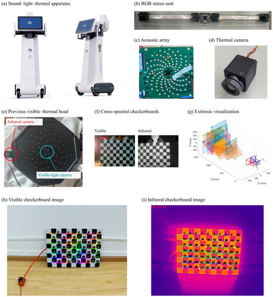
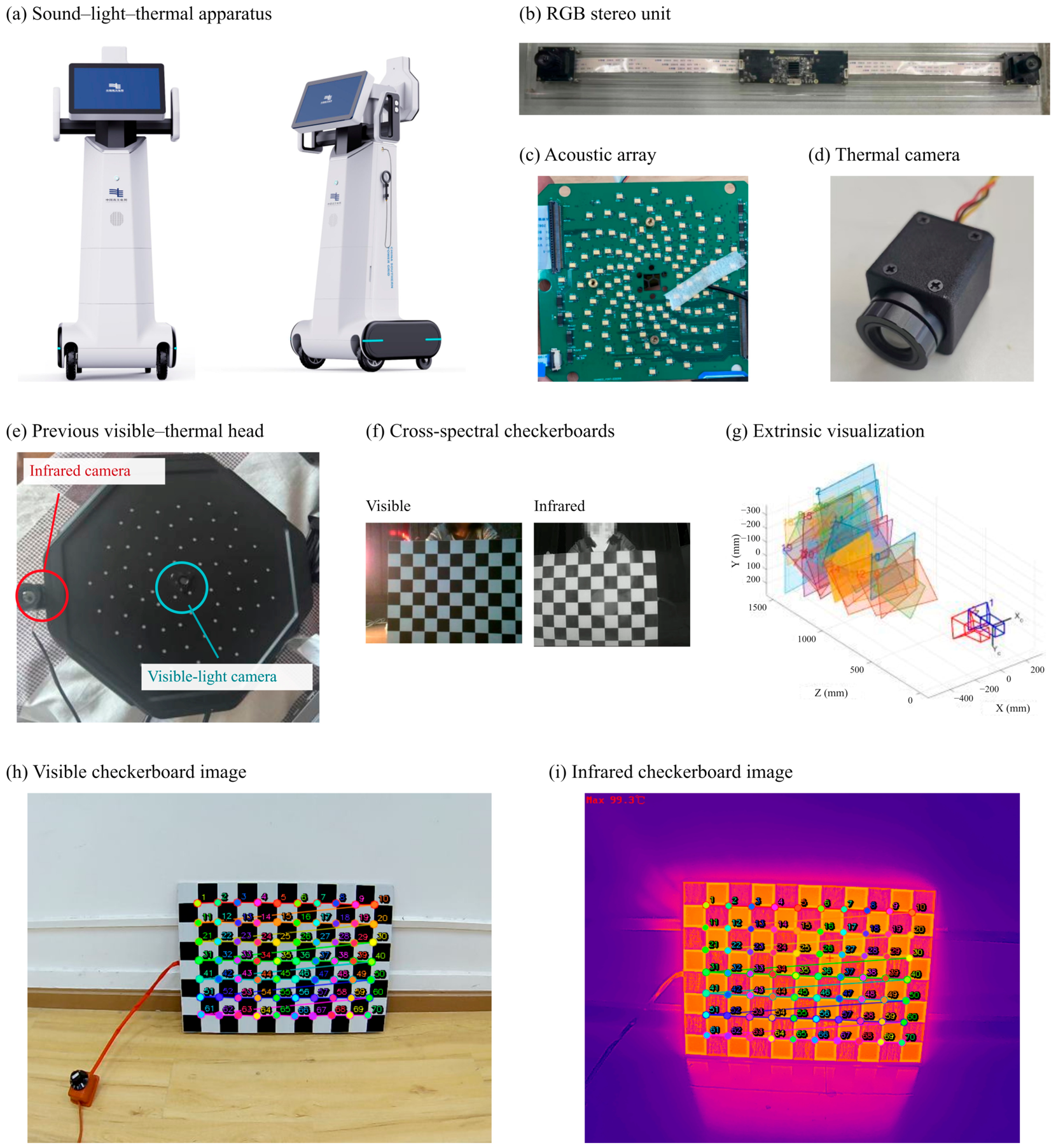
Calibration relates the stereo, thermal-camera, and array frames. Figure 6 shows the apparatus, its sensing units, and the calibration images. Panels (h,i) show a visible–infrared checkerboard with 50 mm squares and a 10-column by 7-row inner-corner grid. The primary evaluation uses noisy and outlier-contaminated 3D–2D correspondences and requires PnP convergence before transport. All 500 cases completed, with zero PnP failures among 100 attempts in each condition and no exclusions. The corresponding one-sided exact 95% upper failure bound is 2.95% per condition. Table S17 reports inliers and reprojection residuals. Table S8 evaluates optional PnP on all 50 supporting cases. Table A5 summarizes the completed supporting-set PnP records.
Figure 6.
Multimodal inspection platform and calibration images: (a) Sound–light–thermal apparatus; (b) RGB stereo unit; (c) Acoustic array unit; (d) Thermal imaging unit; (e) Previous visible–thermal sensing head; (f) Cross-spectral checkerboards; (g) Extrinsic-parameter visualization; (h) Acquired visible checkerboard image; (i) Acquired infrared checkerboard image. Panels (e–g) are reproduced from Figure 2.13 on p. 34 of [33].
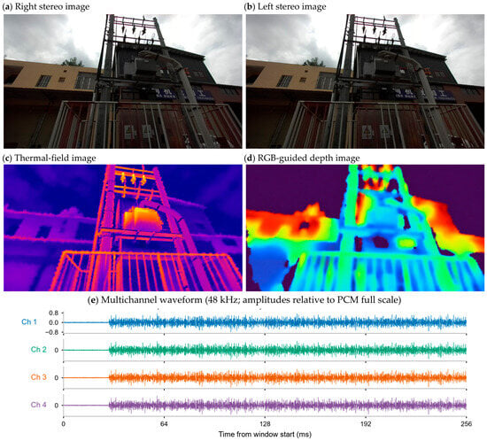
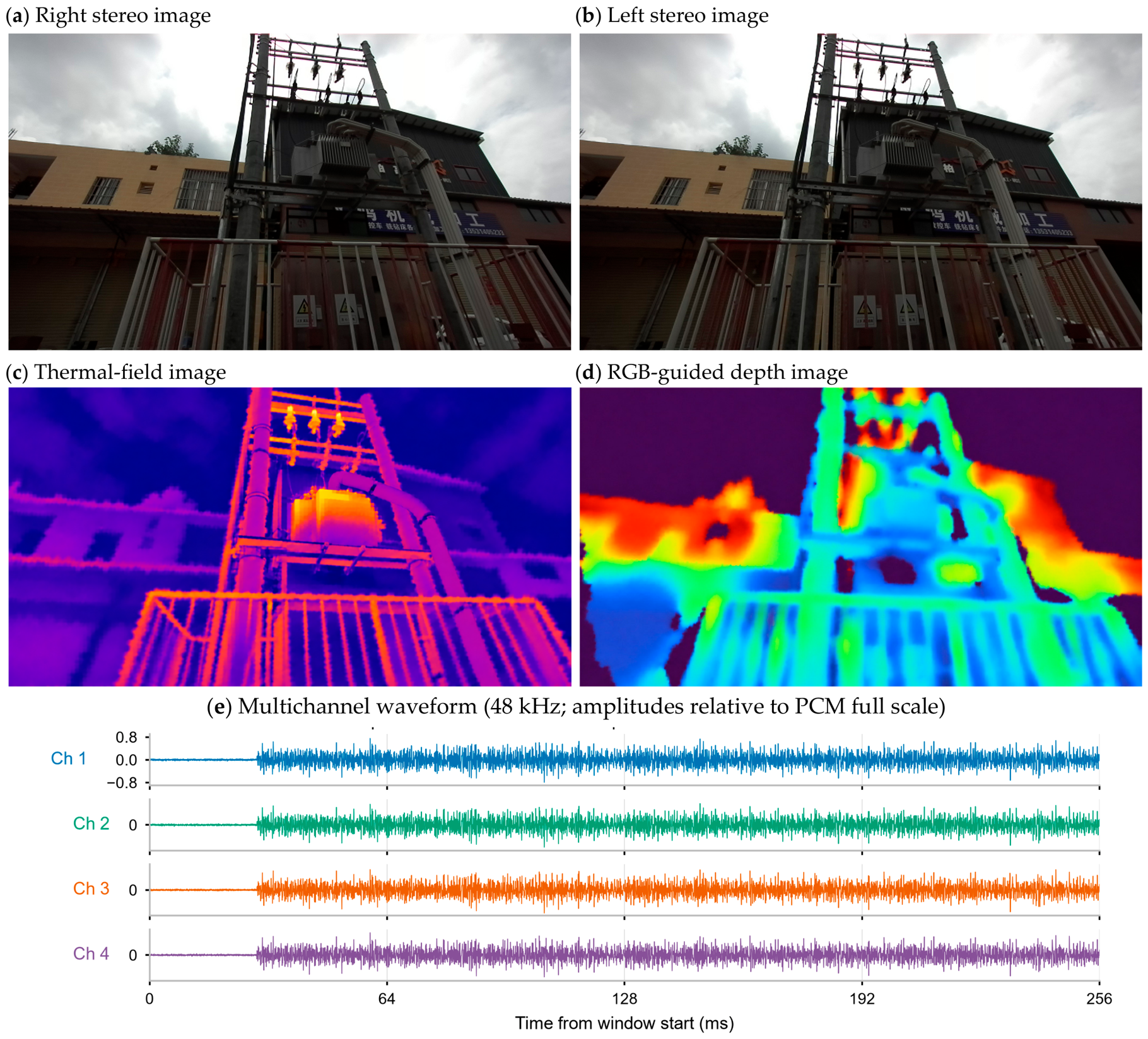
Figure 7 shows the inspection scene and its image and waveform panels.
Figure 7.
Inspection scene and modality representations: (a,b) stereo scene views; (c) thermal-field image; (d) RGB-guided depth image without metric calibration; and (e) numerical multichannel acoustic waveform at 48 kHz, with amplitudes relative to PCM full scale. Panels (c–e) provide visual context and were excluded from the quantitative evaluation.
For the primary evaluation, means give equal weight to case-level rates. Pointwise 95% percentile intervals use 10,000 case-seed bootstrap resamples with master seed 20261112. Paired contrasts resample within-case differences, and identical retained case sets share a resampling stream. Sources and surface nodes are not independent resampling units. Undefined outcomes are reported with their contributing case count; one-case groups receive no inferential interval. The protocol retains every failed attempt without replacement. The supporting-set resampling procedures and seeds are specified separately in Supplementary S1, S12, and S14.
For each acoustic direction with a known reference component, the chance baseline selects uniformly among the distinct component IDs represented by eligible surface nodes. Eligibility follows the candidate-cone and positive-visibility criteria in Section 3.4. The probability of a correct assignment is the reciprocal of the number of eligible component IDs when the reference component is among them, and zero when the reference component is absent or the set is empty. We average these probabilities over all known-reference directions within each case and then over cases, using the same denominator and case weighting as for correct yield.
4.2. Component-Labeled Visible Surface
Table 3 reports geometry for the supporting set. The nominal mean surface error is 37.8 mm and sampled coverage is 35.6%. Its denominator consists of positive reference-component locations on the Cartesian grid formed from surviving sampled coordinates. For the primary set, coverage instead uses a fixed reference grid at the input stride, including positions with no surviving node (Table S18). Primary nominal mean error is 37.57 mm, and coverage is 34.69%. Both coverage measures concern the stereo-visible sampled surface rather than complete equipment area.
Geometry and component masks jointly determine the represented surface. Thin structures and mask errors can remove nodes or assign them to the wrong component. A position error comparable to component separation can change which surface is favored by a thermal projection or acoustic direction. The global mean also conceals local boundary errors. The same-component graph preserves the supplied partition and cannot repair an incorrect mask. Mean errors near 38 mm therefore require particular care for adjacent bushings and terminals; the mask interventions in Section 4.6 quantify one part of this propagation.
4.3. Performance of Thermal and Acoustic Evidence Association
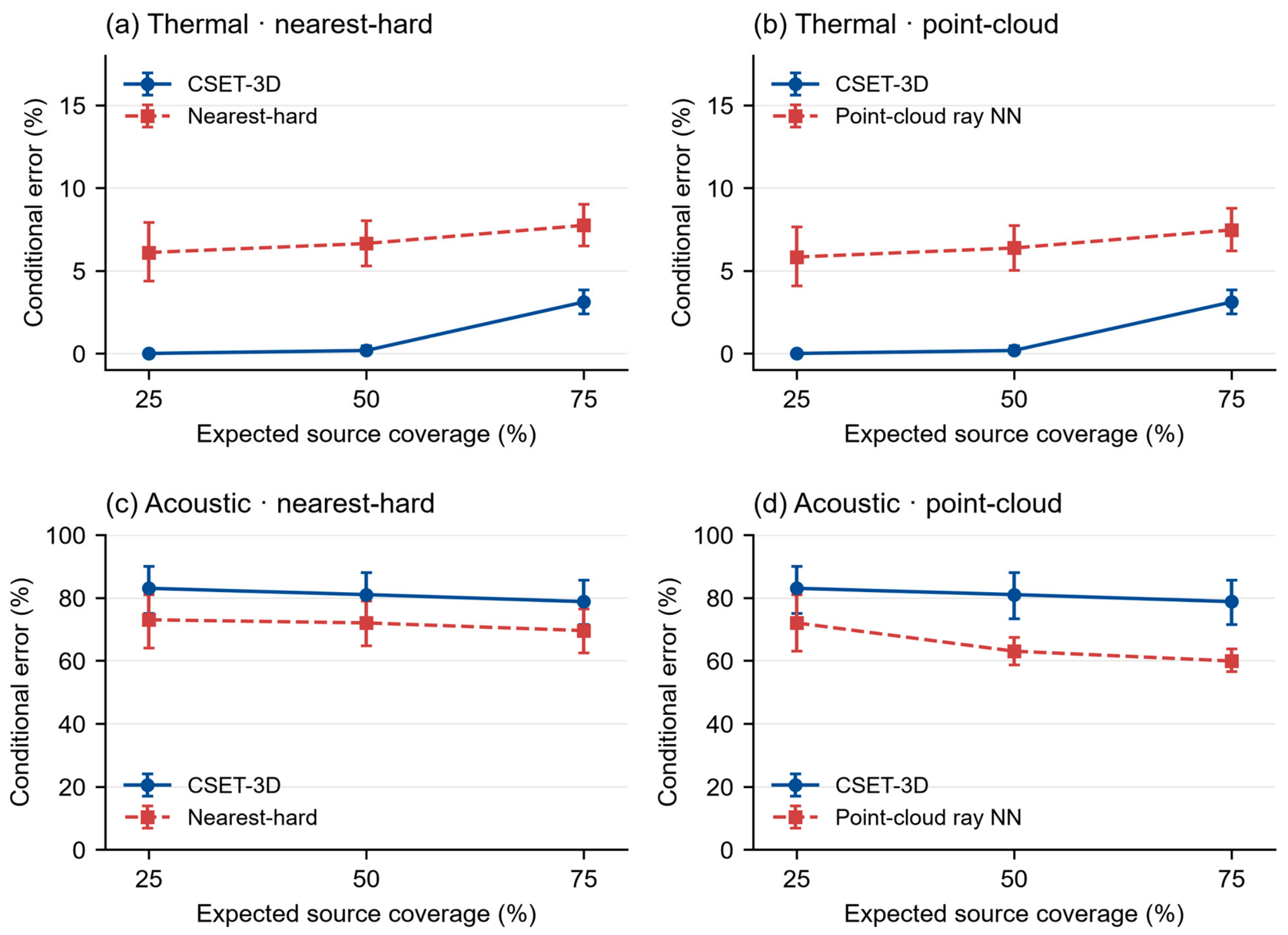
Table 4 reports nominal operating points for the 100 primary nominal cases. Thermal correct yield and admission are 86.55% and 94.11% for CSET-3D, 87.27% and 96.35% for nearest-hard assignment, and 90.15% and 99.91% for the point-cloud comparator. CSET-3D has lower default yield and retention, with 8.03% conditional error. Table 5 and Figure 8 compare selective error at common attainable coverage.
Figure 8.
Reference-based attribution error at common attainable coverage in 100 primary nominal cases: (a,b) thermal and (c,d) acoustic evidence. Comparators are ranked by geometric residual at their selected node. Markers show mean conditional error and pointwise 95% case-bootstrap intervals; lines connect the displayed expected-coverage checkpoints. All 100 pairs reach each displayed checkpoint. The full pAURC comparison in Table 5 uses every attainable integer prefix within each pair’s common range. Reference definitions follow Section 4.1.
In the primary nominal condition, all 300 acoustic directions across 100 cases are admitted, and their candidate sets are nonempty. Uniform assignment among eligible components has an expected correct yield of 12.52%. CSET-3D correctly assigns 71 directions (23.67%), compared with 34.33% for nearest-hard and 37.33% for the point-cloud comparator. For the supporting nominal set, yield is 36.67% under Equation (12) admission (Table S19B) and 33.33% under the component-share criterion (Table S10B).
Selective evaluation ranks nearest-hard assignments by the geometric residual at the selected node: thermal reprojection distance in pixels or acoustic angle in degrees. Smaller residuals rank first, without using reference labels. This ranking leaves assignments and admission unchanged. CSET-3D uses its component-mass score. Table S2 separately evaluates the all-tied nearest-hard component score.
For each case and comparator pair, selective evaluation is restricted to the smaller admitted count. Error is evaluated at each attainable integer prefix; the pAURC sums those risks and divides by the original known-source count. Exact-score ties use expected ordering. Method-specific admitted sets may differ, so matching coverage does not mean selecting identical observations. Unreachable checkpoints remain undefined. Table S2 retains the all-tied diagnostic and detailed common-range definitions.
In the 100 primary nominal cases, the pAURC difference (CSET-3D minus comparator) is −0.0557 [−0.0685, −0.0435] for thermal evidence and +0.0972 [0.0506, 0.1450] for acoustic evidence against residual-ranked nearest-hard assignment. Against the residual-ranked point-cloud comparator, the differences are −0.0521 [−0.0642, −0.0404] and +0.1539 [0.0761, 0.2283]. Each contrast uses 100 paired cases. CSET-3D thus has lower integrated thermal error and higher integrated acoustic error over the respective common attainable ranges.
4.4. Component Descriptors and Mechanism Evidence
Table 6 reports the component descriptor for supporting nominal case 20261001, with 241 nodes and seven represented identities. Thermal values are image-response means over thermal-supported area; acoustic values are relative directional-response means over acoustic-supported area. Support percentages use represented component area, rather than the source-count denominator of admission.
Table 6 note. Thermal values use image-response units; acoustic response and local co-occurrence are dimensionless. Raw-response means use modality-supported area, while support percentages use total represented component area.
Tables S11 and S12 and Figures S4 and S5 report supporting-set allocator contrasts and ablations under the component-share criterion. Removing masks and boundary risk together tests their combined effect. The erosion experiment in Table S4 isolates boundary retreat with fixed references and disparity. Table S6 evaluates the visibility-prior and occlusion-penalty intervention on ten supporting thermal-occlusion cases. These analyses distinguish transport-plan changes from discrete attribution decisions.
Quality ablation changes continuous plans while leaving supporting nominal component assignments and source-admission decisions unchanged (Table S6). Sink suppression changes one component-share acoustic acceptance in a case where all accepted assignments are incorrect, leaving conditional error unchanged. Table A6 reports full-plan sink mass fractions. The fixed-weight and quality-gated softmax controls have the same conditional surface distribution because their cost difference is a common nonsink row penalty.
Timestamp attenuation acts after transport on reliability, not component assignment. In the supporting nominal cases, the thermal offset of about 1.6 ms is small relative to the 50 ms scale in Equation (14), and the acoustic window-center offset is zero relative to its 20 ms scale. Thus the recorded timing factors are close to one; these cases do not test substantial asynchrony. The surface graph links same-component neighbors within a frame and does not track identities across frames.
Tables S3 and S5 report supporting-set parameter sensitivity; Table S16 repeats the specified geometry and transport perturbations on the first 20 primary nominal seeds. These interventions include failed surface constructions and leave the reference settings unchanged. Appendix A gives parameter units and their mathematical roles.
4.5. Controlled Conditions and Computational Cost
Table 7 applies Equation (12) admission to the five primary conditions. Thermal correct yield falls from 86.55% in nominal cases to 37.27% under stereo noise. Acoustic admission is 100% in all five conditions. Under low acoustic SNR, CSET-3D correctly assigns 75 of 300 directions (25.00%), with an expected chance yield of 12.63%. The corresponding nominal yields are 23.67% and 12.52%. Acoustic yield is 35.33% in the thermal-occlusion group. Different conditions use separate case seeds, and geometry within a case is shared across modalities. The condition differences summarize their respective input distributions. Table S22 reports the chance expectations. Tables S13 and S21 report supporting-set results under the component-share and source-admission criteria, respectively.
Shared geometry and calibration can induce correlated modality errors despite separate transport objectives. The calibration-stress condition characterizes the specified transform and timing perturbations; evaluation of long-term field drift would require repeated physical calibration measurements.
For the supporting set, median software-call wall time is 976.4 ms, and median post-run resident memory is 191.5 MiB (Table 8). The associated implementation includes input preparation, reconstruction, allocation, and file/visualization output. A version-bound timing trace is unavailable, so this measurement is treated as aggregate software-call time. Solver-only and acquisition-to-output latency are not inferred. The estimated dense working set is reported separately from measured process memory.
The benchmark uses the workstation in Table 1 and supplied disparity, component identities, and correspondences. Across the 50 supporting cases, median problem size is 238 nodes and 5962 transport pairs. RSS is sampled after each run. Front-end inference, sensing latency, per-stage time, and peak accelerator memory are outside this benchmark.
4.6. Sensitivity Analysis
The primary sensitivity study comprises 1040 case-setting trials: 500 default runs, 300 mask interventions, and 240 parameter interventions. All default and mask runs completed. Of the parameter trials, 220 completed and 20 failed to construct a supported surface at radius 0.04 m. All trials are included in completion counts; undefined geometry and attribution outcomes are reported separately. Input arrays, references, transport plans, and per-source decisions were retained for analysis.
The admission criteria give different counts on the ten supporting nominal cases. The component-share criterion admits 203 thermal sources and Equation (12) admits 205; both correctly assign 190. Acoustic admission changes from 26 to 30 and correct assignments from ten to eleven. These differences follow from the acceptance criteria applied to the same transport plans.
Three controlled mask perturbations are applied to the 100 primary nominal cases. The nearest-centroid pair of positive input components is selected using the input masks. One perturbation merges the smaller region into the larger; two exchange 25% or 50% of each member’s pixels nearest the other centroid. The foreground union, observations, disparity, and reference labels remain fixed while geometry and attribution are recomputed. Partial exchange changes local component membership while retaining the reference identity system.
Relative to each unmodified case, thermal correct yield changes by −0.46 percentage points [−0.74, −0.19] after merging, −0.27 [−0.55, 0.00] after 25% exchange, and −0.32 [−0.64, −0.05] after 50% exchange. Acoustic yield is unchanged in all three interventions. Table S15 also reports admission and conditional-error changes. The small changes describe this localized pair selection; natural segmentation errors can have different extent and geometry.
Radius 0.04 m produces no usable surface in all 20 tested cases. At 0.12 m, mean fixed-grid coverage is 70.00% and mean surface error is 44.14 mm (Table S16). Area-floor changes leave geometry unchanged; normal-angle changes affect graph edges after node construction. Halving sink cost lowers thermal correct yield by 18.51 percentage points [−22.11, −15.13], whereas increasing it by 50% raises yield by 2.73 [1.36, 4.32]. These interventions characterize the sensitivity of the fixed method settings. Table S7 reports the supporting shared-prior comparison.
For new equipment, keep the cost normalization and the source-admission rule fixed while calibrating the thermal sink cost. With the same thermal cost scale, use 3, 6, and 9 as initial settings to compare on separate labeled calibration cases. Choose the setting with the highest correct yield among those meeting the application’s maximum conditional error and minimum source admission. Fix the selected value before evaluation on held-out cases. In the 20 primary nominal sensitivity cases, reducing the thermal sink cost from 6 to 3 lowered correct yield by 18.51 percentage points and source admission by 24.21 percentage points, illustrating why both quantities enter the choice.
5. Discussion
The primary evaluation demonstrates a thermal-retention-error trade-off within the reference-based association task. CSET-3D has lower integrated thermal error over common attainable ranges and lower correct yield at its default operating point. Its admitted, unresolved, and supported states describe where each observation contributes to the exterior-surface representation. Acoustic attribution remains less accurate than the geometric controls.
Component constraints propagate errors in the supplied masks. Supporting-set erosion and primary-set merging or partial identity exchange test different perturbation geometries. Localized changes reduce thermal attribution yield even when the foreground union is unchanged. Acoustic yield is unchanged under these interventions; broader error patterns and real segmentation outputs require separate evaluation.
Thermal response is measured in input-image units. Spatial registration determines its location on the surface. Interpretation as temperature additionally requires radiometric calibration, emissivity, and reflected-radiation information. Cross-camera or cross-session comparisons therefore require a common response scale and known gain, encoding, and contrast processing.
A single acoustic array provides direction without independent range. Multiple labeled surfaces may be compatible with the same direction. Table S9 documents a high-score error caused by concentration of plan mass on a geometrically favored but incorrect component. In the primary nominal comparisons, acoustic pAURC is higher than for both geometric controls. The acoustic output should therefore be interpreted as exploratory exterior-surface association.
The lower thermal pAURC and lower default yield address different operating objectives. The results favor nearest-hard assignment when default retention of correct observations is prioritized. CSET-3D offers lower integrated thermal error over the tested common coverage ranges when selective rejection is acceptable. Selecting a deployment threshold additionally requires application-specific costs for rejection and incorrect attribution. No acoustic performance benefit is observed.
The primary evaluation uses a separate set of random seeds assigned after method settings were fixed. Historical parameter selection and complete attempt records for the supporting set are incomplete. The numerical results characterize the evaluated reference population and the specified input interfaces. Independent physical geometry, source references, and synchronized modality records are unavailable for the Foshan demonstration, as are verified device counts, distances, and loads. Physical attribution, descriptor accuracy, and generalization across equipment therefore remain unvalidated. Bootstrap intervals are pointwise, and intervals containing zero do not establish equivalence.
Learned association methods require compatible inputs and outputs. SuperGlue matches image features [31], whereas GeoTransformer aligns two point clouds [34]. Applying either to this task would require suitable descriptors or a second metric point set, together with a defined conversion to component identities. The present comparisons use a geometric point-cloud association baseline on identical points and masks. Table 9 summarizes the sources of error and their effects on association and reconstruction.
Table 9.
Qualitative error-propagation mechanisms, affected outputs, and methodological controls.
6. Conclusions
CSET-3D associates thermal observations with stereo-visible component surfaces using visibility-aware unbalanced transport, an unresolved destination, and support-aware aggregation. In the nominal computational evaluation, its thermal pAURC over common attainable coverage is lower than for the residual-ranked nearest-hard and point-cloud comparators. Default retention and correct yield are also lower. The exploratory single-array acoustic branch has lower nominal correct yield than both geometric comparators. The mask and parameter interventions quantify attribution sensitivity and geometric failures. The results characterize the selective thermal association trade-off on the modeled exterior surface.
Supplementary Materials
The following supporting information can be downloaded at: https://www.mdpi.com/article/10.3390/en19225595/s1, Figure S1: Auxiliary common-coverage comparison using all-tied component-mass scores for nearest-hard assignment and geometric residual for the gated point-cloud comparator; Figure S2: Geometry and mask sensitivity on ten nominal evaluation cases; Figure S3: Inspection platform in Foshan: (a) indoor electrical-equipment room; (b) roadside pole-mounted equipment; Figure S4: Supporting reference-based results under the component-share criterion: (a) mean surface error and RMSE; (b) sampling-grid coverage; (c,d) unsuccessful attribution versus source coverage; (e,f) conditional accepted-source error versus coverage; Figure S5: Paired ablations on ten supporting nominal evaluation cases under the component-share criterion: conditional accepted-source error for (a) thermal and (b) acoustic evidence; source coverage for (c) thermal and (d) acoustic evidence; Figure S6: Admitted-source risk at common attainable coverage in ten supporting nominal evaluation cases: (a,b) thermal and (c,d) acoustic evidence, compared with nearest-hard assignment and gated point-cloud ray NN; Table S1: Source-admission CSET-3D source counts across all five conditions; ten cases per condition; Table S2: Paired nominal pAURC differences, CSET-3D minus comparator, with the ranking explicitly identified; Table S3: One-factor geometry checks on ten nominal inputs; Table S4: Mask-erosion propagation with unchanged reference labels, percent [95% CI], ten paired nominal cases; Table S5: One-factor transport-parameter sensitivity, percent [95% CI], ten nominal cases; Table S6: Paired source-state changes over ten supporting cases per intervention; Table S7: Joint minus harmonized-separate paired differences, percentage points [95% CI], ten nominal cases; Table S8: PnP outcomes for all supporting-set inputs, with optional refinement; Table S9: Candidate geometry and plan mass for fixed nominal case 20261007, acoustic source index 2; Table S10: Supporting-set association under the component-share criterion; Table S11: Supporting-set paired contrasts under the component-share criterion, CSET-3D minus baseline; Table S12: Paired component-share ablation effects on ten supporting nominal cases; Table S13: Five-condition supporting-set summaries under the component-share criterion; Table S14: Primary-set CSET-3D source inventory; Table S15: Primary-set mask propagation: intervention minus unchanged input, percentage points [pointwise 95% case-bootstrap interval]; Table S16: Parameter interventions on the first 20 primary nominal seeds; Table S17: Required-PnP outcomes for every primary default trial, including all planned cases; Table S18: Primary-set geometry, 100 cases per condition; Table S19: Supporting nominal source-admission operating points, percent [95% CI], ten cases; Table S20: Supporting nominal source-admission paired pAURC differences, CSET-3D minus residual-ranked comparator, ten cases; Table S21: Supporting five-condition source-admission results, ten cases per condition; percent [95% CI]; Table S22: Expected acoustic correct yield under uniform selection among eligible component IDs.
Author Contributions
Conceptualization, W.W.; methodology, W.W. and J.G.; software and formal analysis, J.G.; investigation, Z.L. and X.L.; data curation, Z.L.; validation, X.L.; resources, T.Y. and F.H.; visualization, T.Y.; writing—original draft preparation, W.W.; writing—review and editing, H.X. and F.H.; supervision and project administration, H.X. All authors have read and agreed to the published version of the manuscript.
Funding
This work was supported by the Science and Technology Project of China Southern Power Grid under Grant GDKJXM20231528.
Data Availability Statement
The data that support the findings of this study are available from the corresponding author upon reasonable request.
Conflicts of Interest
Authors Weiguan Wang, Jiahua Guan, Zhongbiao Ling, and Xin Li were employed by the company Foshan Nanhai Power Supply Bureau, Guangdong Power Grid Company Ltd. The remaining authors declare that the research was conducted in the absence of any commercial or financial relationships that could be construed as a potential conflict of interest. The authors declare that this study received funding from Science and Technology Project of China Southern Power Grid. The funder was not involved in the study design, collection, analysis, interpretation of data, the writing of this article, or the decision to submit it for publication.
Appendix A. Implementation Settings
Table A1 specifies numerical floors, geometric settings, and cost and reliability parameters. The 0.08 m radius bounds the local tangent neighborhood; 45° bounds graph-normal variation; the 1 × 10⁻¹⁵ m2 floor rejects degenerate cross-products. Tables S3 and S16 show the support–error behavior of the radius, invariance to much smaller area floors and the graph-only effect of the normal threshold. Tables S5 and S16 characterize sink and entropy sensitivity. All primary default runs retain these settings; the parameter interventions are reported separately.
Table A1.
Parameters, units and computational roles.
The component-parser interface uses a zero mask-logit threshold, a minimum mask score of 0.20, a minimum mask area of 32 pixels, and a 704 × 480 pixel interface resolution. Higher-scoring masks own overlapping pixels. These settings specify the interface; the controlled evaluation does not establish its segmentation accuracy.
Quality enters at distinct locations. Stereo quality is a dimensionless function of photometric and disparity-gradient residuals and contributes to target priors and node reliability. Thermal acquisition quality multiplies source support; the evaluation uses a valid-pixel value of one. Acoustic pair quality is clipped to [0.1, 1], combines with grid quality to form source quality, and controls the angular compatibility scale. Temporal and spatial attenuation act after transport in Equations (14) and (15). None of these scores is calibrated as a probability, measurement variance, or confidence interval.
The sink costs, entropy coefficients, and cost weights in Table A1 come from the original implementation configuration and were fixed for the primary evaluation. The thermal and acoustic sink costs are 6 and 4, and their entropy coefficients are 0.15 and 0.20, respectively. The base pair costs use normalized squared reprojection or angular residuals. The added weights scale depth, boundary, and occlusion penalties in the thermal branch and range–incidence, ambiguity, and boundary penalties in the acoustic branch. The sink costs set the cost of assigning mass to the unresolved destination, and the entropy coefficients control plan smoothness at the respective cost scales. The retained records document the defaults and their roles. The original numerical selection procedure is undocumented.
Table A2.
Method names and software identifiers.
Appendix B. Supporting Reference Definitions and Diagnostics
The supporting set contains ten cases per condition. Each case comprises a reference scene and associated input observations; multiple acoustic peaks share one specified exterior equivalent source. Condition groups use different seed ranges, so cross-condition contrasts compare input distributions rather than paired interventions on a single scene. Table A3 gives the reference-scene settings.
Table A3.
Reference-scene settings for the supporting evaluation set.
Table A4.
Supporting-set CSET-3D source counts under the component-share criterion. Accepted, rejected, and correct counts refer to sources with available reference labels.
Table A4 gives pooled counts, whereas rate summaries weight cases equally. Sources without references are excluded from reference-dependent denominators. At acoustic threshold 0.75, one nominal source is accepted: case 20261007 assigns tank (ID 1) to reference bushing B (ID 6), with score 0.8076 and direction error about 12.05 degrees. Table S9 explains the result through candidate geometry and cost ordering. Thresholds of at least 0.9 admit no supporting nominal acoustic source, giving undefined conditional error.
Table A5.
PnP outcomes in the completed supporting-set records. PnP pose refinement is optional for these inputs. Historical attempts preceding these records are not enumerated.
PnP uses correspondences constructed from the reference geometry. Evaluation of all 50 supporting inputs gives zero failures and no exclusions (Table S8), with optional refinement in their configuration. This denominator covers those 50 inputs; the earlier complete attempt history and learned-feature correspondence failures are not measured.
Table A6.
Full-plan sink mass fractions in the supporting nominal cases. Each fraction is total sink mass divided by total plan mass.
Sink mass fractions and rejected-source counts quantify different outcomes. Source-level ablation results and the effects of the component-share threshold are analyzed in Section 4.4 and Supplementary S7.
References
- Wu, X.; Jiang, L.; Wang, P.-S.; Liu, Z.; Liu, X.; Qiao, Y.; Ouyang, W.; He, T.; Zhao, H. Point Transformer V3: Simpler, Faster, Stronger. In Proceedings of the IEEE/CVF Conference on Computer Vision and Pattern Recognition, Seattle, WA, USA, 17–21 June 2024; pp. 4840–4851. [Google Scholar] [CrossRef] [Scilit]
- Kolodiazhnyi, M.; Vorontsova, A.; Konushin, A.; Rukhovich, D. OneFormer3D: One Transformer for Unified Point Cloud Segmentation. In Proceedings of the IEEE/CVF Conference on Computer Vision and Pattern Recognition, Seattle, WA, USA, 17–21 June 2024; pp. 20943–20953. [Google Scholar] [CrossRef] [Scilit]
- Yilmaz, K.; Schult, J.; Nekrasov, A.; Leibe, B. Mask4Former: Mask Transformer for 4D Panoptic Segmentation. In Proceedings of the IEEE International Conference on Robotics and Automation, Yokohama, Japan, 13–17 May 2024; pp. 9418–9425. [Google Scholar] [CrossRef] [Scilit]
- Evers, C.; Löllmann, H.W.; Mellmann, H.; Schmidt, A.; Barfuss, H.; Naylor, P.A.; Kellermann, W. The LOCATA Challenge: Acoustic Source Localization and Tracking. IEEE/ACM Trans. Audio Speech Lang. Process. 2020, 28, 1620–1643. [Google Scholar] [CrossRef] [Scilit]
- Zhang, T.; Zhang, H.; Li, X.; Chen, J.; Lam, T.L.; Vijayakumar, S. AcousticFusion: Fusing Sound Source Localization to Visual SLAM in Dynamic Environments. In Proceedings of the IEEE/RSJ International Conference on Intelligent Robots and Systems, Prague, Czech Republic, 27 September–1 October 2021; pp. 6868–6875. [Google Scholar] [CrossRef] [Scilit]
- He, Y.; Shin, S.; Cherian, A.; Trigoni, N.; Markham, A. Sound3DVDet: 3D Sound Source Detection Using Multiview Microphone Array and RGB Images. In Proceedings of the IEEE/CVF Winter Conference on Applications of Computer Vision, Waikoloa, HI, USA, 4–8 January 2024; pp. 5496–5507. [Google Scholar] [CrossRef] [Scilit]
- He, Y.; Shin, S.; Cherian, A.; Trigoni, N.; Markham, A. SoundLoc3D: Invisible 3D Sound Source Localization and Classification Using a Multimodal RGB-D Acoustic Camera. In Proceedings of the IEEE/CVF Winter Conference on Applications of Computer Vision, Tucson, AZ, USA, 28 February–4 March 2025; pp. 5408–5418. [Google Scholar] [CrossRef] [Scilit]
- Wen, B.; Dewan, S.; Birchfield, S. Fast-FoundationStereo: Real-Time Zero-Shot Stereo Matching. In Proceedings of the IEEE/CVF Conference on Computer Vision and Pattern Recognition, Denver, CO, USA, 3–7 June 2026; pp. 7513–7524. Available online: https://openaccess.thecvf.com/content/CVPR2026/html/Wen_Fast-FoundationStereo_Real-Time_Zero-Shot_Stereo_Matching_CVPR_2026_paper.html (accessed on 27 September 2026).
- Wen, B.; Trepte, M.; Aribido, J.; Kautz, J.; Gallo, O.; Birchfield, S. FoundationStereo: Zero-Shot Stereo Matching. In Proceedings of the IEEE/CVF Conference on Computer Vision and Pattern Recognition, Nashville, TN, USA, 11–15 June 2025; pp. 5249–5260. [Google Scholar] [CrossRef] [Scilit]
- Lipson, L.; Teed, Z.; Deng, J. RAFT-Stereo: Multilevel Recurrent Field Transforms for Stereo Matching. In Proceedings of the International Conference on 3D Vision, London, UK, 1–3 December 2021; pp. 218–227. [Google Scholar] [CrossRef] [Scilit]
- Xu, G.; Wang, X.; Ding, X.; Yang, X. Iterative Geometry Encoding Volume for Stereo Matching. In Proceedings of the IEEE/CVF Conference on Computer Vision and Pattern Recognition, Vancouver, BC, Canada, 18–22 June 2023; pp. 21919–21928. [Google Scholar] [CrossRef] [Scilit]
- Hirschmüller, H. Stereo Processing by Semiglobal Matching and Mutual Information. IEEE Trans. Pattern Anal. Mach. Intell. 2008, 30, 328–341. [Google Scholar] [CrossRef] [Scilit] [PubMed]
- DeTone, D.; Malisiewicz, T.; Rabinovich, A. SuperPoint: Self-Supervised Interest Point Detection and Description. In Proceedings of the IEEE/CVF Conference on Computer Vision and Pattern Recognition Workshops, Salt Lake City, UT, USA, 18–22 June 2018; pp. 224–236. [Google Scholar] [CrossRef] [Scilit]
- Lindenberger, P.; Sarlin, P.-E.; Pollefeys, M. LightGlue: Local Feature Matching at Light Speed. In Proceedings of the IEEE/CVF International Conference on Computer Vision, Paris, France, 1–6 October 2023; pp. 17627–17638. [Google Scholar] [CrossRef] [Scilit]
- Li, J.; Hu, Q.; Ai, M. RIFT: Multi-Modal Image Matching Based on Radiation-Variation Insensitive Feature Transform. IEEE Trans. Image Process. 2020, 29, 3296–3310. [Google Scholar] [CrossRef] [Scilit] [PubMed]
- Tuzcuoğlu, Ö.; Köksal, A.; Sofu, B.; Kalkan, S.; Alatan, A.A. XoFTR: Cross-Modal Feature Matching Transformer. In Proceedings of the IEEE/CVF Conference on Computer Vision and Pattern Recognition Workshops, Seattle, WA, USA, 17–18 June 2024; pp. 4275–4286. [Google Scholar] [CrossRef] [Scilit]
- Nguyen, D.-L.; St-Charles, P.-L.; Bilodeau, G.-A. Non-Planar Infrared-Visible Registration for Uncalibrated Stereo Pairs. In Proceedings of the IEEE Conference on Computer Vision and Pattern Recognition Workshops, Las Vegas, NV, USA, 26 June–1 July 2016; pp. 63–71. [Google Scholar] [CrossRef] [Scilit]
- Zhang, T.; Hu, L.; Sun, Y.; Li, L.; Navarro-Alarcon, D. Computing Thermal Point Clouds by Fusing RGB-D and Infrared Images: From Dense Object Reconstruction to Environment Mapping. In Proceedings of the IEEE International Conference on Robotics and Biomimetics, Jinghong, China, 5–9 December 2022; pp. 1707–1714. [Google Scholar] [CrossRef] [Scilit]
- Knapp, C.H.; Carter, G.C. The Generalized Correlation Method for Estimation of Time Delay. IEEE Trans. Acoust. Speech Signal Process. 1976, 24, 320–327. [Google Scholar] [CrossRef] [Scilit]
- Cobos, M.; Antonacci, F.; Alexandridis, A.; Mouchtaris, A.; Lee, B. A Survey of Sound Source Localization Methods in Wireless Acoustic Sensor Networks. Wirel. Commun. Mob. Comput. 2017, 2017, 3956282. [Google Scholar] [CrossRef] [Scilit]
- Cobos, M.; Martí, A.; López, J.J. A Modified SRP-PHAT Functional for Robust Real-Time Sound Source Localization with Scalable Spatial Sampling. IEEE Signal Process. Lett. 2011, 18, 71–74. [Google Scholar] [CrossRef] [Scilit]
- Ma, M.; Ren, J.; Zhao, L.; Testuggine, D.; Peng, X. Are Multimodal Transformers Robust to Missing Modality? In Proceedings of the IEEE/CVF Conference on Computer Vision and Pattern Recognition, New Orleans, LA, USA, 18–24 June 2022; pp. 18177–18186. [Google Scholar] [CrossRef] [Scilit]
- Han, Z.; Yang, F.; Huang, J.; Zhang, C.; Yao, J. Multimodal Dynamics: Dynamical Fusion for Trustworthy Multimodal Classification. In Proceedings of the IEEE/CVF Conference on Computer Vision and Pattern Recognition, New Orleans, LA, USA, 18–24 June 2022; pp. 20707–20717. [Google Scholar] [CrossRef] [Scilit]
- Geifman, Y.; El-Yaniv, R. Selective Classification for Deep Neural Networks. Adv. Neural Inf. Process. Syst. 2017, 30, 4878–4887. Available online: https://papers.nips.cc/paper_files/paper/2017/hash/4a8423d5e91fda00bb7e46540e2b0cf1-Abstract.html (accessed on 27 September 2026).
- Peng, Y.; Li, H.; Wu, P.; Zhang, Y.; Sun, X.; Wu, F. D-FINE: Redefine Regression Task of DETRs as Fine-Grained Distribution Refinement. In Proceedings of the International Conference on Learning Representations, Singapore, 24–28 April 2025; Available online: https://openreview.net/forum?id=MFZjrTFE7h (accessed on 27 September 2026).
- Fischler, M.A.; Bolles, R.C. Random Sample Consensus: A Paradigm for Model Fitting with Applications to Image Analysis and Automated Cartography. Commun. ACM 1981, 24, 381–395. [Google Scholar] [CrossRef] [Scilit]
- Lepetit, V.; Moreno-Noguer, F.; Fua, P. EPnP: An Accurate O(n) Solution to the PnP Problem. Int. J. Comput. Vis. 2009, 81, 155–166. [Google Scholar] [CrossRef] [Scilit]
- Yang, J.; Yan, W.; Yuan, S.; Yu, Y.; Mao, Z.; Chen, R. Image Fusion and Target Detection Based on Dual ResNet for Power Sensing Equipment. Sensors 2025, 25, 2858. [Google Scholar] [CrossRef] [Scilit] [PubMed]
- Cuturi, M. Sinkhorn Distances: Lightspeed Computation of Optimal Transport. Adv. Neural Inf. Process. Syst. 2013, 26, 2292–2300. Available online: https://papers.nips.cc/paper/2013/hash/af21d0c97db2e27e13572cbf59eb343d-Abstract.html (accessed on 27 September 2026).
- Chizat, L.; Peyré, G.; Schmitzer, B.; Vialard, F.-X. Scaling Algorithms for Unbalanced Optimal Transport Problems. Math. Comput. 2018, 87, 2563–2609. [Google Scholar] [CrossRef] [Scilit]
- Sarlin, P.-E.; DeTone, D.; Malisiewicz, T.; Rabinovich, A. SuperGlue: Learning Feature Matching with Graph Neural Networks. arXiv 2019, arXiv:1911.11763. [Google Scholar] [CrossRef] [Scilit]
- Jiang, Q.; Liu, Y.; Yan, Y.; Deng, J.; Fang, J.; Li, Z.; Jiang, X. A Contour Angle Orientation for Power Equipment Infrared and Visible Image Registration. IEEE Trans. Power Deliv. 2021, 36, 2559–2569. [Google Scholar] [CrossRef] [Scilit]
- Zhang, Y. Holographic Imaging Based Hazard Source Detection and Representation Methods for Electrical Public Safety. Doctoral Dissertation, Wuhan University, Wuhan, China, 2026; p. 34, Figure 2.13. [Google Scholar]
- Qin, Z.; Yu, H.; Wang, C.; Guo, Y.; Peng, Y.; Xu, K. Geometric Transformer for Fast and Robust Point Cloud Registration. arXiv 2022, arXiv:2202.06688. [Google Scholar] [CrossRef] [Scilit]

Disclaimer/Publisher’s Note: The statements, opinions and data contained in all publications are solely those of the individual author(s) and contributor(s) and not of MDPI and/or the editor(s). MDPI and/or the editor(s) disclaim responsibility for any injury to people or property resulting from any ideas, methods, instructions or products referred to in the content. |
© 2026 by the authors. Licensee MDPI, Basel, Switzerland. This article is an open access article distributed under the terms and conditions of the Creative Commons Attribution (CC BY) license.