


Abstract
From the end of 2020, every new building in the European Union had to be a nearly zero-energy building (nZEB). Afterwards, new-dwelling prices grew faster than existing-dwelling prices in most countries. The European Central Bank linked part of this growth differential to energy costs and other factors. Its energy explanation is tested against a phase shift of new-dwelling prices (later recording or slower adjustment) and the cyclical sensitivity of existing dwellings, with country, cross-country, panel and event-study estimates for 26 Member States (without Greece). After correction for multiple testing, the differential shows no association with national energy indicators: energy prices, heating fuels, nZEB values and carbon intensity of electricity, which alone nears significance before correction. Much of the measured rise is a matter of timing. Between 2019–2021 and 2022–2025 the differential rose more where building permits fell more, consistent with a cyclical account, but the rise and this link largely disappear when new-dwelling prices are compared with existing-dwelling prices two or four quarters earlier. The contemporaneous differential thus overstates the lasting change in relative prices. The asymmetry itself is not new: in 2007–2014, before any nZEB requirement, existing dwellings fell further than new ones in most countries. The timing of national rate increases does not identify a credit channel. Energy premia are better estimated within the existing stock, and segment comparisons should allow for the phase shift.
1. Introduction
The European Union (EU) set a common deadline for nearly zero-energy buildings (nZEB) but not a common standard. Under Article 9(1)(a) of the Energy Performance of Buildings Directive of 2010, every new building had to be a nearly zero-energy building from 31 December 2020 [1]. When the Buildings Performance Institute Europe (BPIE) analyzed the national rules half a year later, it found a numerical indicator of primary energy use for single-family houses in 21 Member States and two Belgian regions, from 27 kWh/m2 a year in Denmark to 158 in Romania [2]. Article 9(3)(a) of the Directive required such an indicator, hereafter the national nZEB value.
Within two years, prices of new and existing dwellings moved apart. In the euro area, annual growth of existing-dwelling prices had been half a percentage point above that of new dwellings at the peak of the cycle. At the trough it was “around 6 percentage points lower”, a larger difference than in the global financial crisis and the sovereign debt crisis [3]. This difference between the annual growth rates of the two segments is referred to as the growth differential.
The authors of this European Central Bank (ECB) analysis relate the differential to the fading of an earlier exuberance in purchases of existing dwellings, to the growing weight of energy costs in buyers’ choices, and to two cost factors. The first is related to supply: new dwellings had been built when construction was expensive, so there were “limits to lowering prices”. The second concerns older buildings, whose sale may depend on prior renovation. In their view, the cost of such renovation and the hesitance of potential buyers also help to explain why prices of existing dwellings fell much more than those of new dwellings. It is the energy side of this account, the link between energy performance and the differential, that is tested in this paper. This link does not appear to have been tested across the Member States so far. In Poland, where the growth differential also shifted in early 2021 [4], a single national index cannot separate the nZEB requirement from the other shocks of the period; for this reason, the comparison here covers 26 Member States.
Only the deadline was the same. The shocks around it differed, beginning with the timing of monetary tightening. Czechia and Hungary raised their policy rates in June 2021, Poland and Romania in October 2021 and Sweden in the second quarter of 2022, while the ECB and Danmarks Nationalbank followed in July 2022 [5,6]. Between the first halves of 2021 and 2023, household gas prices rose by between 8% in Hungary and 508% in Lithuania, and between 2021 and 2023 building permits collapsed in Sweden, whereas in Spain they grew. The common deadline thus met national and regional housing markets in different phases of the cycle, so the episode is examined across countries and, for Poland, across cities. These differences help to separate the energy explanation from a cyclical one. If energy performance determines the differential, it should follow the energy shock. Conversely, if the segments simply go through the cycle differently, it should follow the cycle.
Growth rates alone cannot identify the source of the shift, because the competing explanations predict the same rise and differ only in where, when and in which segment it should appear. Two alternatives to the energy explanation follow from the stock-flow model of the housing market [7] and from the way the house price index records new dwellings, which in many Member States enter it at the deed rather than at the contract, with a recording lag between the price agreement and its recording in the index. They lead to three hypotheses.
H1.
The faster growth of new-dwelling prices after 2021 was part of the housing downturn and was larger in the Member States where housing construction contracted more.
H2.
Much of the faster growth of new-dwelling prices after 2021 reflects a phase shift, in which new-dwelling prices follow the market with a delay because pre-sold dwellings enter the index at the deed or because developers adjust their prices more slowly.
H3.
Existing dwellings are the segment more sensitive to the housing cycle, so in the downturn of 2007–2014, before any nZEB requirement, their prices fell further than those of new dwellings in real and in nominal terms, by more than a recording lag can produce.
The energy explanation of the ECB analysis is the subject of the first research question. In addition, four questions concern monetary policy transmission and the Polish case, since the Polish shift motivated the study and the energy structure of Poland differs from that of its neighbors.
RQ1.
Does the energy performance of buildings explain why new-dwelling prices rose faster relative to existing-dwelling prices in some Member States than in others, i.e., is the rise larger where the energy shock was stronger, where more of the stock is heated with fossil fuels or depends on carbon-intensive electricity, and where the national nZEB value is stricter?
RQ2.
Are existing-dwelling prices more sensitive to interest rates than new-dwelling prices once shocks common to all Member States are allowed for?
RQ3.
Did the differential rise in response to each country’s own monetary tightening?
RQ4.
Does the Polish shift, measured on two independent price sources, follow the European pattern?
RQ5.
Does the energy structure of Poland, including its position relative to the break-even carbon intensity of electricity for heat pumps, set it apart from its neighbors in the Union and leave a mark on the differential?
The hypotheses and the first research question are tested with different kinds of evidence, namely the energy variables and building permits across the Member States with a correction for the number of variables tested, a comparison of new-dwelling prices with existing-dwelling prices of earlier quarters, which shows how much of the measured differential reflects a delay in new-dwelling prices rather than a change in their relative value, and the real decline of each segment after 2021 and after 2007, when the nZEB requirement was not yet in force. Each hypothesis is subjected to more than one test.
Energy premia have so far been estimated within single markets, and, in the literature reviewed, the recording lag has been measured directly only in two Polish cities, but a single price series cannot show whether a faster rise of new-dwelling prices reflects a premium for energy performance, a difference in cyclical sensitivity between the segments or a misalignment of the two indices in time, since all three predict the same rise. The contribution of the paper lies in separating these three explanations, each confronted with evidence that the other two do not predict, i.e., the variation in energy shocks, construction and monetary timing across Member States, the alignment of the two series in time and a downturn that preceded the nZEB requirement. The answer matters for energy policy, because a faster rise in the price of new dwellings can be read as the market value of a stricter energy standard, and the zero-emission and renovation requirements of Directive (EU) 2024/1275 [8] will again change the energy performance of both segments.
2. Three Explanations and Their Predictions
2.1. One Market, Two Segments
Models of the housing market, hedonic studies of energy performance and work on house price indices each yield one prediction about where and when the differential should appear. The property market can be divided into a market for space and a market for assets, which the stock-flow model links through construction [7]. Prices are formed in the asset market, and construction responds to the price of a dwelling relative to the cost of building it. Because one year’s construction adds only a thin layer to the stock, the stock itself changes slowly.
In a supply-determined model of housing investment in the United States, the one-quarter elasticity of new housing supply is about 1.0 and the long-run elasticity about 3.0 [9]. In the cost-based approach, new construction is minimal where prices fall below the minimum profitable production cost [10]. The asset-market approach to owner-occupied housing draws a similar line between the market for existing houses and the market for new construction. In this model, the price of the stock is set by the discounted value of housing services, and gross investment rises with that real price [11]. In a model in which construction responds to changes in prices and costs rather than to their levels, a 10% rise in real prices adds 0.8% to the housing stock through a temporary 60% increase in starts spread over four quarters [12]. Where supply is elastic, booms are fewer and shorter, and after a boom prices return towards construction costs [13].
The models reviewed above lead to the first prediction of the present study. When credit tightens, the asset value of housing falls, and existing dwellings, supplied from the stock, adjust mostly through price. In contrast, new dwellings are a flow produced at a cost, and hence their adjustment goes mostly through quantity, i.e., through fewer permits and starts. As a result, the growth differential should rise more where the downturn is deeper.
In the hedonic model, a dwelling is treated as a bundle of characteristics, each with its own implicit price [14], and energy performance is one of them. When energy becomes more expensive, the present value of the savings brought by efficiency rises, and this leads to the second prediction. If the differential after 2021 reflects a rise in the implicit price of energy performance, it should be larger where energy prices rose more. Under the same explanation, the differential should also be larger where more of the existing stock is heated with fossil fuels or, less clearly, depends on carbon-intensive electricity, and where the national nZEB value separated new from old buildings more sharply. The same rise would also appear as a discount on inefficient existing dwellings, the channel stressed in the ECB analysis; it is the pattern across countries and over time, rather than the segment that moves, that sets this prediction apart.
The third prediction concerns measurement. New dwellings are often sold before completion, and where the index records them at the deed, it may reflect prices agreed months or even years earlier [15]. As a result, such an index lags behind the index of existing dwellings, and in a downturn part of any measured differential may then be a matter of phase. If this is the case, the differential should shrink once the two series are aligned in time, as the timing of a falling market shows (Figure 1).
Figure 1.
Recording of prices of existing and pre-sold new dwellings in a falling market. Source: own elaboration based on Statistics Poland [16].
For an existing dwelling, the price agreement and the deed are usually close in time, so the index follows the market with a short delay. By contrast, for a new flat sold before completion, the price may be agreed before construction begins, and multi-family buildings completed in Poland in 2024 took 26.0 months to build on average [16]. The deed, and with it the index, can then record a price set two years earlier. In a falling market, the index of new dwellings keeps showing earlier, higher prices for longer, and a differential appears even if both markets moved together at the moment of contract. In nominal terms, a recording lag of fixed length delays both the peak and the trough of the new-dwelling index without making the fall shallower, whereas a lag that varies between transactions averages prices agreed in different quarters and makes the fall shallower as well. In real terms, it can also change the measured depth, because a nominal price recorded later is divided by a later consumer price level. Similarly, a phase shift would also arise if developers adjusted their prices more slowly than sellers of existing dwellings.
2.2. Energy Performance in House Prices
Most hedonic studies find that buyers pay for energy performance. Of 68 European studies published up to May 2024, about three-quarters report a positive effect and none a negative one, with each additional energy performance certificate band worth roughly 1–3% [17]. The energy price shock of 2022 changed this premium unevenly. Belgian label premia changed little between 2016 and 2022 and rose in 2023–2024 [18], and in Norway, in the regions affected by the electricity price shock of 2021–2022, house prices fell by 1.2–3.6% on average and those of energy-efficient homes fell less [19]. In Germany, dwellings below class A lost ground against the most efficient ones, in both asking prices and asking rents, once energy became expensive [20]. In Hungary, the estimated market value of energy-inefficient property was about 12% below that of property with an average rating before the change in household energy tariffs of August 2022 and about 20% below it afterwards [21]. Likewise, the premium of Norwegian homes rated A or B over class C grew from around 8% to 13% after 2022 [22].
However, the hedonic studies of recent years treat the two segments in different ways. Two studies leave new buildings out of their main estimates [18,23]; one covers only new housing projects [24]; one, on rents, runs separate models by dwelling condition [25]; one reports results by year of construction [20]; and one compares Norwegian regions with different exposure to the electricity price shock [19]. The others pool new and existing dwellings and control for construction year or condition [21,22,26]. Consequently, none of these studies separates an energy component of the price difference between new and existing dwellings.
In Poland, the energy intensity of multi-family buildings has been built into models of apartment values [27], but for Poland, Slovakia and Lithuania no peer-reviewed estimate of the energy premium based on data for 2021–2024 has been found. The clearest evidence on a stricter standard comes from Massachusetts, where towns that adopted a stretch energy code saw a price premium for efficient homes and fewer new single-family starts [28]. A stricter code may therefore raise the relative price of new dwellings in two ways, through the demand for efficiency and through a smaller supply of new homes. How strict the national requirements are, however, differs between Member States. Poland set a national nZEB value of 70 kWh/m2 a year for single-family houses, Lithuania 60, Slovakia 54 and Czechia 130, while Austria, Flanders, Germany, Italy, Luxembourg and Portugal gave no number and defined the standard through a reference building [2].
2.3. The Segments over the Cycle and in the Index
Studies of single markets support the first and third predictions. In one US metropolitan area, new homes sell at a premium over comparable existing homes mainly when few new homes are supplied [29]. In the 17 largest Polish cities, prices on the secondary market respond to the real interest rate more than twice as strongly as prices on the primary market [30]. For Warsaw and Poznań, the index of existing dwellings has been found to lead the index of new dwellings by up to two years, because new units sold before completion enter the data only at the deed [15]. In Warsaw, rising prices of small and medium second-hand flats also preceded rising prices of larger newly built ones [31], and across Polish cities the ratio of primary-market to secondary-market prices fluctuates irregularly [32], with strong spillovers between the two markets [33].
In Norway, the relative price growth of new homes moves with developers’ inventory-to-sales ratios, which points to prices that adjust more slowly than those of existing homes [34]. In France, the indices of new and second-hand dwellings differ in path and volatility, partly because land weighs more in the price of second-hand dwellings [35]. The Czech National Bank reported a similar pattern for late 2022. In its assessment, prices of lower-quality and prefabricated flats fell, whereas those of higher-quality flats, including new developments, stagnated, and slow construction kept the supply of new flats tight [36].
Two models suggest why the existing stock may be the more sensitive segment. In a model with a minimum down payment, households that sell one dwelling to buy another depend on the equity they hold in the first one. The model connects this constraint with the volatility of prices and with the positive correlation between prices and trading volume [37]. A model of the property ladder adds that credit constraints delay first purchases and that the capital gains or losses of constrained owners of starter homes make prices of trade-up homes the most volatile [38]. Such owners may be more common among buyers of existing dwellings than among buyers of new ones. Spectral analyses of prices in Ireland and the United Kingdom point the same way, since second-hand prices in Ireland carry an additional cycle attributed to repeat buyers [39], and new housing is the less volatile segment [39,40]. A third mechanism works against a nominal fall: for Boston condominiums, owners facing a nominal loss set higher asking prices and sell less often [41]. Asymmetric adjustment of this kind, linked to loss aversion and nominal rigidity, has also been found in Polish regional markets over 2000–2022 [42]. When inflation is high, prices of existing dwellings can therefore fall in real terms while barely moving in nominal terms, and for this reason the depth of a downturn in the two segments is better compared after deflation.
Monetary policy reaches housing supply slowly and unevenly. A temporary one-percentage-point rise in the short-term interest rate reduces euro-area housing investment by around 5% after about three years [43]. Indeed, in the third quarter of 2025, housing investment was still about 7% below its peak of early 2022 [44]. For building permits, the long-run semi-elasticities with respect to the mortgage rate lie between −20% and −26% per percentage point in Germany and between −14% and −23% in France [45].
At the level of the euro area, prices of existing dwellings rose 0.8 percentage points faster than those of new dwellings in 2020, a year of rising prices [46], i.e., in the opposite order to that of 2022–2024. The methods of the national indices themselves differ [47]. However, none of the studies reviewed compares new and existing dwellings across the Member States after the common nZEB deadline, confronts the energy explanation of the differential with the stock-flow model and the recording lag, or repeats the comparison for an earlier downturn.
2.4. Research Framework
The three predictions can be tested against one another because they disagree about where, when, and in which segment the differential should appear. Under the energy explanation (the second prediction), the differential should follow the size of the energy shock and the strictness of the national nZEB value, and there is no reason to expect it before the nZEB requirement is applied. If the differential reflects a phase shift (the third prediction), it should shrink once the two series are aligned in time [15]. Under the cyclical explanation (the first prediction), which also draws on credit constraints, the differential should rise more where the downturn is deeper, and existing dwellings should fall further in real terms in any downturn, including one that preceded the requirement. The hypotheses and research questions follow from these predictions and are placed in the stock-flow framework of the study (Figure 2).
Figure 2.
Stock-flow framework of the study. Source: own elaboration; solid arrows: cyclical explanation and recording lag; dashed arrows: energy explanation and research questions.
The upper part of the scheme shows the cyclical explanation and the recording lag, in which monetary tightening lowers the asset value of housing, existing dwellings adjust through price, and new dwellings adjust through quantity and, where recorded at the deed, enter the index later. The lower part shows the energy explanation, which works through the implicit price of energy performance, and the measured differential lies between the two.
H1 concerns the construction cycle. Both the cyclical explanation and a phase shift predict that the rise in the relative price of new dwellings, which adjust through quantity [9,12], should be largest where construction contracted most, whereas the energy explanation predicts it only if a stricter standard itself held back construction [28]. Permits brought forward before the deadline, the size of the preceding boom, which could have inflated the base from which permits fell [13], and trends that predate the tightening must be ruled out as the source of this pattern.
Timing is the subject of H2. Whether pre-sold dwellings enter the index only at the deed [15] or developers adjust their prices more slowly than sellers of existing dwellings, new-dwelling prices follow the market with a delay, which in a downturn raises them relative to existing ones for a time, most where the market turned most sharply. Both mechanisms, one of measurement and one a genuine rigidity of developers’ prices, imply that comparing new-dwelling prices with existing-dwelling prices of an earlier quarter should remove most of the measured rise, its link with construction and the part of the deeper real fall of existing dwellings that only reflects the delay, and that the order of the two segments should reverse in an upswing, as it did in 2020.
H3 concerns the segments themselves. If existing dwellings adjust through price and credit-constrained owners [37,38] are concentrated in their market, real prices of existing dwellings should fall further than those of new dwellings in any downturn. As a property of the housing market rather than of the regulation, such an asymmetry should already appear in the downturn of 2007–2014, before the nZEB requirement. It should then also appear in nominal terms, since inflation was far lower than in 2022–2023, and in the Member States in which the existing series does not lead the new one, where a recording lag has little room to smooth the new-dwelling index.
RQ1 concerns the energy explanation of the ECB analysis [3]. Its prediction, the second of the three, holds whether the rise appears as a premium for new dwellings or as a discount on inefficient existing ones. RQ2 and RQ3 ask whether the tightening that preceded the downturn can be identified as its source, either through a stronger response of existing-dwelling prices to interest rates, as found for Polish cities [30], or through the timing of national rate increases. RQ4 and RQ5 apply the comparison to Poland, on two price sources and against its neighbors in the Union.
3. Data and Empirical Strategy
The empirical strategy follows from the disagreements between the three predictions. A single measure of the differential would carry its own weakness into every test. Year-on-year growth rates depend on the moment at which transactions are recorded, a cross-section of 26 countries is small, and a shock that hit all Member States in the same quarter cannot be distinguished from the common deadline. Therefore, the evidence is collected across the Member States, within them over time and, for Poland, across cities and on two independent price sources. The energy variables enter cross-country and panel regressions of the same form as the measures of the construction cycle, and the competing explanations are thus examined with the same tools. The design runs from public data, through three measures of the relation between the two segments, namely the growth differential, real peak-to-trough declines and responses to interest rates, to tests that examine each hypothesis in more than one way (Figure 3).
Figure 3.
Research design. Source: own elaboration.
Read by rows, the research design also shows how each test is checked. Because RQ1 and H1 rest on at most 26 countries, they are checked with rank correlations and permutation tests and, within countries, in the panel. H2 repeats the country estimates and the real declines with the existing-dwelling series shifted back, a benchmark of what a pure recording lag would produce. H3 compares deflated price levels in a downturn that preceded the nZEB requirement, which means that it depends neither on growth rates nor on the period of the deadline. RQ2 compares the segments in a stacked panel with common and with segment-specific quarter effects, and for RQ3 an event study is complemented by an estimator that compares only with countries not yet treated.
3.1. Sources and Variables
House prices come from the house price index that Eurostat publishes quarterly for purchases of newly built and of existing dwellings [48]. The split is available for 26 Member States (Greece is not covered), with series starting between 2005 and 2010. The study period is 2015 Q1–2025 Q4, with the regressions on interest rates starting in 2016 Q1, and only the comparison of real declines in the downturn of 2007–2014 uses earlier data. For each segment, the year-on-year (y-o-y) rate of change is used, and the growth differential is defined as the rate for new dwellings minus the rate for existing dwellings, in percentage points (p.p.). For Poland, Eurostat publishes the price indices of residential premises of Statistics Poland [49], and over 2019 Q1–2025 Q4 the two sets of values differ by no more than 0.2 percentage points. The annual item weights of the index give the shares of new and existing dwellings in all 26 countries [50].
The national annexes to the Eurostat metadata state when a purchase of a newly built dwelling enters the index [51]. In 11 countries it is the deed or the transfer of ownership (Belgium, Bulgaria, Ireland, Italy, Latvia, Malta, Poland, Portugal, Romania, Slovakia and Spain), and in 10 the sale or reservation contract (Austria, Croatia, Cyprus, Finland, France, Germany, Hungary, Lithuania, the Netherlands and Slovenia). The remaining five follow mixed or different practices, among them Denmark, which proxies new dwellings with construction cost indices, and Sweden, which dates them at the start of construction. The other three are Czechia, Estonia and Luxembourg. All five are kept in the estimation of the leads and in the comparisons with the existing series shifted back, which do not use the classification by recording practice. However, they are left out of Fisher’s exact test and of the split by recording practice, and the cross-country results are also reported without them.
Construction activity is represented first by building permits, measured as the number of dwellings in residential buildings, except residences for communities, quarterly and unadjusted [52]. Construction producer prices for the same category of buildings enter as year-on-year changes [53], because a construction cost index is not published for all countries. In addition, the year-on-year change in the calendar-adjusted volume of production in construction for buildings, hereafter construction output, available for 23 countries, mostly up to 2023 Q4, is a second measure of activity [54].
Daily central bank policy rates come from the Bank for International Settlements (BIS) [5]. For the euro area, the deposit facility rate of the ECB is used throughout [55], the rate through which the ECB steers its monetary policy stance [56]. Similarly, Croatia and Bulgaria, whose currencies were tied to the euro, are assigned the euro-area rate throughout. For Denmark, the series is the rate on certificates of deposit of Danmarks Nationalbank, without the technical adjustment of 19 March 2021 [57], which the cut of 1 October 2021 reversed [58], and the first Danish increase is thus that of 22 July 2022 [6]. Mortgage rates are measured, wherever the sources allow, as rates on pure new loans, i.e., on new business without renegotiated loans. For nine euro-area countries (Austria, Estonia, Finland, France, Germany, Latvia, Lithuania, the Netherlands and Slovakia) they come from the ECB statistics on interest rates of monetary financial institutions, available from August 2017 [59]. For Poland, Czechia and Hungary, they come from Narodowy Bank Polski (NBP), the Czech National Bank and the Magyar Nemzeti Bank [60,61,62].
The energy variables begin with half-yearly household prices of natural gas and electricity, including all taxes and levies, in purchasing power standard (PPS) per kWh [63,64]. The fuel structure of household space heating refers to 2023 [65]. The carbon intensity of electricity generation, as lifecycle grams of CO2 equivalent per kWh, comes from Ember [66,67]. National nZEB values for single-family houses are taken from the BPIE review [2], which gives none for the five Member States that rely on a reference building, Austria, Germany, Italy, Luxembourg and Portugal, and no national value for Belgium, whose regions follow different approaches. To compare the depth of the downturn in real terms, both price indices are deflated by the harmonized index of consumer prices (HICP, all items, 2015 = 100), averaged over the three months of each quarter [68].
For Poland, two further sources are used. The BaRN database of NBP (Baza cen nieruchomości mieszkaniowych) gives quarterly mean transaction prices per square meter on the primary and secondary markets of 17 cities, at least one in every voivodship, compiled from data supplied by estate agents and developers, with quarters shifted by one month, the first running from December to February [69]. The Local Data Bank of Statistics Poland gives median prices per square meter of residential premises sold in market transactions, by market, for the same 17 cities up to 2024 Q4 [70].
3.2. Country Estimates and Cross-Country Analysis
The first set of estimates compares, country by country, the growth of the two price indices before and after the nZEB deadline. The pre-treatment period runs from 2019 Q1 to 2021 Q4 and the post-treatment period from 2022 Q1 to 2025 Q4. The window is offset by a year after the deadline because of the development cycle of new dwellings. For each Member State, the change in the growth differential is then estimated with Equation (1):
where yst is the year-on-year rate of change of the index for segment s in quarter t; News equals 1 for newly built and 0 for existing dwellings; Postt equals 1 from 2022 Q1 and 0 before; β0 is the mean pre-treatment growth of existing dwellings, β1 the pre-treatment growth differential, β2 the shift common to both segments and β3 the change in the growth differential, in percentage points; εst is the error term.
Standard errors are clustered by quarter, with p-values based on normal critical values, and Newey–West standard errors with four lags allow for the overlap of year-on-year rates of quarterly data [71]. For every country, the pre-treatment linear trend of the differential and the estimate for a treatment date of 2021 Q1 are also reported. Since existing dwellings are hit by the same credit and energy shocks, react differently to interest rates [30], and differ in location, age, and condition, they are a comparison group only in a descriptive sense. The coefficient β3 therefore describes the change in the growth differential rather than an effect of the nZEB requirement; the name difference-in-differences refers only to the form of the estimator.
For H2, the existing-dwelling series is replaced by its value one, two, three, four, and eight quarters earlier, and the cross-country relation with permits is re-estimated for each shift and, for shifts of two and four quarters, with the change in the log ratio of the new-dwelling to the existing-dwelling index between 2019–2021 and 2022–2025, which does not rest on overlapping growth rates. The lead of the existing series in each country is the lag, of up to eight quarters, at which the correlation of its year-on-year rate with that of the new-dwelling series over 2015–2025 peaks. Because it is estimated on the period studied, the lead is also estimated on the quarters before 2020 and assessed with a moving-block bootstrap, and its link with the official recording practice is tested with Fisher’s exact test. These shifts are the same for every country and do not depend on the estimated lead. The lead is used only to divide the countries, and this division is repeated in each bootstrap draw of the leads.
A shift of the existing series measures how much of the differential is a matter of phase, but it cannot distinguish a recording lag from a slower adjustment of developers’ prices, because both delay the new-dwelling index in the same way. As a placebo, the treatment date is moved to 2020 Q1 on data for 2018 Q1–2021 Q4.
Next, the 26 estimates of β3 are regressed, one variable at a time, on country characteristics that correspond to the three predictions. The permit measures are the change in the annual mean of the building permit index between 2021 and 2023 and the same change measured from 2019. A third, the mean year-on-year change in permits in 2020 Q4 and 2021 Q1, measures permits brought forward around the deadline, i.e., an anticipation effect of the requirement. The other variables are the mean growth of construction producer prices in 2021 and 2022, the cumulative policy-rate increase in the tightening cycle and five energy variables, namely the carbon intensity of electricity in 2022, the share of fossil fuels (solid fossil fuels, natural gas, and oil and petroleum products) in space heating in 2023, the national nZEB value, available for 20 countries, and the changes in household gas and electricity prices in PPS between the first halves of 2021 and 2023. The second and third measures guard against applications filed before the deadline inflating the 2021 base, as in Poland, where the dwellings for sale or rent covered by permits or registrations in December 2020 were almost double the monthly mean of the preceding eleven months [72].
Heteroskedasticity-consistent (HC1) standard errors are used, together with Spearman’s rank correlation, a permutation test and leave-one-out estimates. For the energy variables of RQ1, the p-values of the rank correlations are adjusted for the number of variables with the Holm method [73], and, as a check, over all ten country characteristics. The 90% confidence intervals of Spearman’s correlation are based on Fisher’s z transformation with the standard error of Bonett and Wright [74]. The real annual growth of existing-dwelling prices between 2015 Q4 and 2021 Q4 and, separately, the pre-treatment trend of the differential are added as controls, so that the permit measure of H1 does not stand in for the preceding boom or for earlier trends.
3.3. Panel and Event Study
A comparison of two periods around a single date says nothing about what moves the differential from quarter to quarter. The panel therefore uses every quarter and relates the differential to national conditions after removing what all Member States shared in each quarter. It covers the 26 Member States from 2015 Q1 to 2025 Q4, and the baseline specification is Equation (2):
where Diffit is the growth differential of country i in quarter t, in percentage points; αi and λt are country and calendar-quarter fixed effects; Xit is one regressor at a time, with coefficient γ; and εit is the error term. The regressors are the change in the policy rate over the preceding four quarters, contemporaneous or lagged by two or four quarters; the year-on-year change in building permits, contemporaneous or lagged, and also with construction output as a control; construction producer prices; the year-on-year change in the household gas price; and the interaction of an indicator of the post-2020 period, equal to 1 from 2021 Q1 onwards, with the national nZEB value centered on the Polish 70 kWh/m2 a year. In further regressions, the year-on-year change in permits becomes the dependent variable, and for 12 countries the policy rate is replaced by the rate on new mortgage loans. Standard errors are clustered by country, again with normal critical values. Because 26 clusters are few and the policy rate varies only across seven central banks, the wild cluster restricted bootstrap with Webb weights is also reported for the main coefficients [75,76], with clustering by country and, for the policy rate, by central bank. With the seven central banks as clusters, all 279,936 possible bootstrap samples are enumerated, and as these clusters are of very unequal size, these p-values are indicative. In the event study for RQ3, Xit is replaced with indicators of the quarter relative to the first increase of the national policy rate after 2020, as in Equation (3):
where Ditk equals 1 if quarter t lies k quarters from the first increase in country i and θk is the differential in that quarter relative to the quarter before the increase (k = −1). Relative quarters are binned at −8 and +12. First increases define four cohorts: 2021 Q2 for Czechia and Hungary, 2021 Q4 for Poland and Romania, 2022 Q2 for Sweden, and 2022 Q3 for Denmark and the euro area, whose rate is also assigned to Croatia and Bulgaria. Since every country is eventually treated and 21 of the 26 share one date, a fully dynamic specification is under-identified without never-treated units [77]. Because the two-way fixed-effects (TWFE) coefficients may also mix in comparisons with countries already treated [78,79], the interaction-weighted estimator of Sun and Abraham [78] is also reported, with the last-treated cohort (2022 Q3) as the comparison group and the sample ending in 2022 Q2, before this cohort is treated. Each comparison is thus made with countries not yet treated, i.e., it is a clean comparison in the terminology of Roth et al. [79]. Similarly, the estimator of Callaway and Sant’Anna [80] uses only clean comparisons and would run into the same short post-treatment window.
3.4. Real Declines and Interest-Rate Sensitivity
The country estimates and the cross-country regressions rest on year-on-year growth rates, which show when prices moved but not how far each segment fell from its previous peak, and it is the depth of the fall that the cyclical explanation is about. For country i and segment s, with Pist the price index deflated by the HICP, the largest real peak-to-trough decline over a window is given by Equation (4):
where the inner maximum is the highest value of the deflated index within the window up to quarter t. For the recent downturn, the window runs from 2021 Q1 to 2025 Q4, and the calculation is repeated from 2020 Q1 and in nominal terms, with the quarters of the peak and of the trough recorded. For H3, the window runs from 2007 Q1 to 2014 Q4 and covers the 19 Member States whose indices for both segments start by 2008 Q1. The two declines are compared with the Wilcoxon signed-rank test and the sign test, in real and in nominal terms. For the recent downturn, a bootstrap interval for the median difference is also reported, together with the results without the three smallest markets (Cyprus, Luxembourg and Malta). Because each segment has its own peak and trough, the two declines need not span the same quarters. Both downturns are therefore also compared over a common window, from the peak to the trough of the deflated index for all dwellings in each country, over which both segments are measured.
For H2 and H3, both windows are recomputed with a benchmark of the recording lag, in which the existing-dwelling index of quarter t − L, for L = 2 and L = 4, is compared with the new-dwelling index of quarter t, both deflated by the HICP of quarter t. If the two segments moved together at the moment of contract and only the recording of new dwellings came later, this benchmark would reproduce the real decline of the new-dwelling index, so an asymmetry that reflects recording should disappear in it, whereas one that reflects a difference in cyclical sensitivity should remain.
Because a lag that varies between transactions also makes the fall shallower, the benchmark is repeated with the existing-dwelling index of quarter t replaced by its mean over quarters t − K to t, for K = 2, 4 and 8. Since such smoothing would also delay the new-dwelling index, the countries are also divided by the estimated lead of the existing series. Where the two series correlate most closely with no lag, a recording lag could smooth the new-dwelling index only slightly, and how much it could do so is assessed with a simulation in which the new-dwelling index is generated as a distributed lag of the existing one (Appendix A). As a check that does not depend on the estimated lead, the countries are also divided by their official recording practice, deed or contract. For both downturns pooled, the difference between the two declines is regressed on an indicator of a lead, an indicator of the recent downturn, and their interaction, with standard errors clustered by country.
Real declines do not show the link with interest rates that RQ2 asks about. For this question, the two segments are stacked in one panel, as in Equation (5):
where yist is the year-on-year change of the price index of segment s in country i and quarter t, μis are country-by-segment fixed effects, λt calendar-quarter effects common to both segments and xit the change in the interest rate over the preceding four quarters. News equals 1 for new dwellings, and εist is the error term. β measures the response of existing-dwelling prices and β + δ that of new-dwelling prices, so δ > 0 means that new dwellings respond less negatively. Because λt cancels in the difference between the segments, δ also draws on movements of rates and of the differential shared by all Member States, which is why Equation (5) is also estimated with calendar-quarter effects specific to each segment, which compare only countries in the same quarter. The mortgage rate is used for 12 countries and the policy rate for all 26, contemporaneous and lagged by two quarters, with standard errors clustered by country. For δ, the wild cluster restricted bootstrap with Webb weights is added [75,76], with clustering by country and, for the policy rate, also by the seven central banks. Estimates that leave out one country at a time are also reported. All estimates were computed in R.
3.5. Polish Cities and the Break-Even Carbon Intensity
Below the national level, RQ4 is examined in Polish cities. The country estimate of Equation (1) is repeated on BaRN transaction prices for its aggregates of seven and ten cities and for each of the 17 cities, with heteroskedasticity-consistent (HC3) and quarter-clustered standard errors. The same is repeated on the median prices of Statistics Poland for the same cities, with the post-treatment period ending in 2024 Q4.
Whether a heat pump lowers emissions depends on the carbon intensity of the electricity used, relative to the emissions of the gas boiler that it is compared with. The break-even carbon intensity of electricity [4], below which the heat pump emits less than the boiler, follows from equating the emissions per kWh of heat of the two systems, g/SCOP for the heat pump and fgas/η for the boiler, and enters here as Equation (6):
where g is the carbon intensity of electricity, SCOP the seasonal coefficient of performance of the heat pump, set equal to the seasonal performance factor measured in the field, fgas the emission factor of natural gas, and η the seasonal efficiency of the boiler. The value of fgas is 0.200 kg CO2 per kWh [81], and η is 0.86 for a boiler with an atmospheric burner and 0.91 for a condensing boiler [82]. SCOP is set to 2.5, the lower end of the seasonal performance factors recorded in field monitoring of air-to-water heat pumps in existing buildings [83,84]. With this value, g must stay below 581 g CO2 per kWh against the first boiler and below 549 g against the second, and the first, more lenient value is used as the break-even intensity. Because heat pumps installed in new buildings often perform better, the break-even intensity is also given for SCOP of 3.0 and 3.5. The comparison matters for RQ5 because the nZEB requirement favors electric heat pumps in new buildings, and the emissions they save depend on the national electricity mix. Annual Ember intensities are used for the comparison of Poland with its neighbors in the Union, because they are computed in the same way for every country. Ember reports lifecycle values, whereas fgas covers direct combustion only, and the comparison is thus tilted against the heat pump.
4. Evidence on the Three Explanations
4.1. The Differential Across the Union and by Country
The first step is descriptive. It asks whether the relative price of new dwellings changed after the deadline at all, and whether it did so in the Union as a whole or only in some Member States. All three explanations expect the measured differential to widen after 2021, but they disagree about its source. Under the energy explanation, new dwellings would gain value relative to older and less efficient ones, or older ones would lose it. Under the cyclical explanation, existing dwellings would lose more in the downturn, and under a phase shift, new units, priced before the downturn, would show the fall later. Yet the aggregate series cannot decide between them. It does show when the differential widened, how large it became, and how long it lasted. Between 2015 and 2020 the quarterly growth differential of the EU-27 stayed between −1.8 and +0.4 percentage points (Figure 4).
Figure 4.
House price index of the EU-27 by segment and growth differential, year-on-year change, 2015 Q1–2025 Q4. Source: own elaboration based on Eurostat [48].
For six years the two segments moved in step. From 2021 they separated, first in one direction and then, more strongly, in the other. In annual terms, existing dwellings still grew faster in 2021, the order reversed in 2022, and in 2023 prices of existing dwellings fell by 1.6% on average over the year, while prices of new dwellings rose by 5.0%. Because existing dwellings carry about four-fifths of the weight of the EU-27 index, the index for all dwellings barely fell that year.
The lines in the figure did not move in the same way. Growth of new-dwelling prices slowed after its peak in 2022 but remained positive in every quarter, whereas growth of existing-dwelling prices was negative throughout 2023 and turned positive again only in 2024. Thus, the rise of the differential came mainly from the existing segment. The slowdown of existing-dwelling prices was steepest at the turn of 2022 and 2023, in the first quarters after the ECB began to raise its rates. Since the energy explanation also allows for a discount on older dwellings, this pattern alone does not decide between the explanations, but it argues against a shift of demand that would have accelerated new-dwelling prices in 2023, when the differential widened most.
By 2024 the differential had narrowed, and in 2025 it turned slightly negative; the episode thus lasted about three years. According to Equation (1), the rise amounts to 3.83 percentage points for the EU-27 and to 2.82 for the euro area, with p < 0.001 in both cases. Country by country, the estimate for the 2022 Q1 treatment date is positive in 19 of the 26 Member States (Table 1).
Table 1.
Difference-in-differences estimates of the growth differential by Member State, 2019 Q1–2025 Q4 (percentage points).
In 13 countries, the estimate is positive and significant at the 10% level, from Sweden, Latvia, Romania and Denmark at the top down to Czechia and Finland. With Newey–West standard errors, 11 of them remain significant, all except Sweden and Latvia. Portugal is the only country with a significant negative estimate. The median is 2.25 percentage points. On Eurostat values, the Polish estimate is 5.77, i.e., practically the same as the 5.80 obtained from the figures of Statistics Poland [49]. Poland and the four Member States bordering it all belong to the group with positive and significant estimates. However, they are served by three central banks that began to tighten at different times: Czechia in June 2021, Poland in October 2021 and Germany, Slovakia and Lithuania, as members of the euro area, in July 2022.
Moreover, pre-treatment trends go in both directions, with Cyprus and Hungary at the two extremes, and are steep in several countries, among them Sweden and Latvia. With the treatment date moved to 2021 Q1, the estimates keep much of their order but are smaller in most countries, and five, all among the countries with small or negative estimates for 2022 Q1, become significantly negative. Finally, the placebo date of 2020 Q1 gives eight estimates significant at the 10% level, of which only one, for Hungary, is positive. With so many significant placebo estimates, the number of significant country estimates is better read as a description of the episode than as a test.
4.2. Energy Variables and the Differential
The country estimates differ by more than eleven percentage points between Cyprus and Sweden, and this spread is the material for RQ1. If the differential reflects a rise in the implicit price of energy performance, the largest estimates should come from the countries where the energy shock was strongest, where more of the stock is heated with fossil fuels or depends on carbon-intensive electricity, and where the national nZEB value drew a sharper line between new and old buildings. The five energy variables are related to β3 in the same way as the measures of the construction cycle and of the tightening, one at a time and with the same inference, so that none of the explanations is favored by the design. None of the five energy variables is significantly related to β3, and the largest share of its cross-country variance that any of them explains is 9% (Table 2).
Table 2.
Cross-country regressions of the difference-in-differences estimate on country characteristics.
This is not due to a lack of variation in the energy variables. The share of fossil fuels in space heating ranges from 1% in Sweden to 92% in Ireland, and the carbon intensity of electricity ranges from 41 to 733 g CO2e per kWh, while the national nZEB values and the rise in household gas prices vary just as widely (Table A1). Nor is the gas price shock, a priori the most relevant energy variable, significantly related to β3. Among the rank correlations, only that of the carbon intensity of electricity comes close to significance (p = 0.052). None of them passes the Holm adjustment, none of the least-squares slopes passes the permutation test, and among their 90% intervals only that of the carbon intensity of electricity excludes zero (Table A2). Its sign is negative, i.e., the estimates are smaller where electricity is more carbon intensive. The energy explanation does not fix the sign of this variable firmly, because new buildings heated with electricity depend on the same electricity mix as old ones, which means that this correlation does not support the energy explanation either.
The confidence intervals of the slopes also show which effects the data leave room for. A doubling of the household gas price goes with a change in β3 of between −0.2 and 1.3 percentage points (95% interval), and a national nZEB value stricter by 10 kWh/m2 a year with a change of at most about 0.4 points, whereas a fall in permits larger by 10 percentage points goes with an estimate higher by about half a point.
Nor does the cost factor of the same account [3] explain the estimates. Construction producer prices enter with a negative sign, i.e., where these prices rose faster, the differential grew less, but this slope rests largely on Bulgaria and is not significant without it.
Within countries over time, the energy variables leave no trace. In the panel of Equation (2), country effects remove permanent national differences, such as the age and composition of the stock, and calendar-quarter effects remove what all Member States went through together, including the deadline itself and the common part of the energy shock. What remains is national timing. If the energy explanation holds, the differential should widen in the quarters in which national gas prices rise and, after 2020, more where the national nZEB value is stricter. However, neither of these variables is significantly related to the differential, and neither are construction producer prices (Table 3).
Table 3.
Panel regressions of the growth differential, 26 Member States, 2015 Q1–2025 Q4.
Both energy coefficients are small and carry the sign opposite to the one that the energy explanation implies. The differential is, if anything, narrower in quarters of faster gas-price growth and, after 2020, wider where the nZEB value is less strict. As regards RQ1, the variables of the energy explanation do not account for the differences between countries, nor do they follow the differential within countries. The energy performance of the dwellings that enter the two indices is not observed, which makes this a result about national energy indicators. It does not show that energy performance plays no part in the prices of individual dwellings or in the differential, and nZEB values, set for single-family houses, are missing for six countries and not defined in the same way in the others [2].
4.3. Timing of the Two Price Series
Unlike the energy variables, the change in building permits between 2021 and 2023 is closely related to the country estimates (Figure 5). It explains 31% of the cross-country variance of β3 (Table 2), with a rank correlation of −0.62. The permutation test confirms the least-squares slope, and leaving out any one country keeps it clearly negative (Table A2). Measured from 2019, the change in permits is still related to β3, and the measure of permits brought forward, related to larger estimates on its own, loses significance once the change in permits enters the same regression, while the permit coefficient barely moves. Moreover, the placebo estimates for 2020 Q1 do not depend on the change in permits.
Figure 5.
Difference-in-differences estimates and the change in building permits, 26 Member States. Source: own calculations based on Eurostat [48,50,52]; bubble area: share of new dwellings in the house price index, 2021.
The real growth of existing-dwelling prices before 2022 is related neither to β3, once permits are controlled for, nor to the change in permits, and with this variable or the pre-treatment trend in the regression, the permit coefficient stays at −0.055. The rank correlation also remains significant without Denmark and Sweden, whose new-dwelling indices are built from construction costs and from the start of construction, or without all five countries with a mixed or different practice. It also survives the Holm adjustment over all ten country characteristics, unlike any of the other variables. These results are consistent with H1 but do not show that the fall in permits caused the differential, since permits and prices respond to the same market conditions and the cross-section has only 26 observations.
As Figure 5 shows, Sweden, Denmark and Germany, where permits fell by 64%, 43% and 36%, are among the six countries with the largest estimates. By contrast, Finland (−52%) and Estonia (−36%) lie well below the fitted line. Seven countries issued more permits in 2023 than in 2021, and six of them have estimates close to zero or negative, the exception being Slovenia. All seven lie in the south and south-east of the Union, from Portugal and Spain to Cyprus and Bulgaria, where the number of permits did not fall during the tightening. Poland is placed next to Germany and Romania, with permits about 30% lower.
Membership of the euro area does not order the scatter. Estonia, Latvia and Lithuania share the policy rate of the ECB, yet Estonia lies well below the fitted line and Latvia well above it. The weight of new dwellings in the index is largest in Malta and Cyprus, about three-quarters and two-thirds, and both countries have negative estimates. This weight is not significantly related to β3 (rank correlation −0.23), meaning that the size of the new segment in the index does not by itself account for the estimates.
However, a relation of this kind is also what a recording lag would produce, which is why timing is examined directly. In 13 countries the two series correlate most closely with no lag, and in the other 13 the existing series leads, by one quarter in Luxembourg, two in Estonia, Finland, Lithuania and the Netherlands, four in Denmark, Ireland and Latvia, five in Sweden and eight, the longest lead examined, in Italy, Malta, Poland and Romania.
In 2015–2025, these leads are related to the official recording practice. Of the eight countries in which the existing series leads by four quarters or more, all six with a deed or contract practice record new dwellings at the deed or the transfer of ownership, namely Ireland, Italy, Latvia, Malta, Poland and Romania, whereas none of the ten countries that record them at the contract has a lead longer than two quarters (Fisher’s exact test, p = 0.012). The leads are, however, estimated imprecisely in a moving-block bootstrap, and those estimated before 2020, when prices moved less, do not reproduce the link with recording practice (Appendix A). When new-dwelling prices are compared with existing-dwelling prices of earlier quarters, both the rise and its relation with permits largely disappear (Table 4).
Table 4.
Difference-in-differences estimates with the existing-dwelling series shifted back, 26 Member States, 2019 Q1–2025 Q4.
With a shift of two quarters, the median estimate in Table 4 falls from 2.25 to 0.64 percentage points, and only four estimates remain positive and significant. With four quarters, the median is close to zero. The relation with permits weakens in the same way. With a two-quarter shift, the slope falls to about a third and loses significance, and the rank correlation, at −0.35, is significant only at the 10% level. With four quarters, both change sign, and so does the rank correlation of the change in permits with the change in the log relative price of new dwellings. With eight quarters, a shift longer than the lead found in all but four countries, the relation is reversed and significant, which is what too long a shift would produce if the differential were a matter of phase. Of the six estimates that stay above 3 percentage points with a two-quarter shift, five belong to countries where the existing series leads by four quarters or more, namely Romania, Poland, Latvia, Denmark and Sweden, and the exception is Germany.
These results do not depend on the lead estimated for each country, because the same shift is applied to all of them. With shifts of one and three quarters, the median estimate and the slope on the change in permits lie between those of the neighboring shifts, and the estimates thus decline steadily as the shift lengthens rather than at one particular lag. How uncertain the lead is matters only for the division of the countries. Although the estimated lead recurs in a median of 61% of the bootstrap draws, the countries with a lead of four quarters or more keep a lead of at least two quarters in 92% of them. Recording at the deed and slower adjustment of developers’ prices both delay the new-dwelling index; hence the results support a timing explanation, a phase shift between the two indices, without identifying its mechanism.
Within countries, in line with H1, the differential widens by 0.024 percentage points for every percentage point by which the year-on-year growth of national permits falls in the same quarter, a coefficient that survives the wild cluster bootstrap and a control for construction output (Table 3). In contrast, permits lagged by two quarters show no relation, and at four quarters the sign changes. A contemporaneous association is what a common turn of the market would produce, recorded at once in permits and in existing-dwelling prices and only later in the prices of new dwellings. The alternative measures of construction point to the same conclusion. Measured from 2019, the fall in permits explains 16% of the cross-country variance of β3 instead of 31%, and with construction output as a control the within-country coefficient is −0.033. A link that holds in the same quarter but not with permits lagged by two or four quarters, and that disappears once the existing series is shifted back, is consistent with a cyclical account in which permits and prices respond to the same conditions, but it does not establish that the decline in permits caused the differential.
4.4. Real Declines in Two Downturns
The existing series shifted back shows how much of the result on growth rates is a matter of phase. A growth differential can also widen because existing dwellings fall further, which would be a difference in cyclical sensitivity, measured here on price levels deflated by consumer prices. Real values are used because owners facing a nominal loss tend to hold their asking prices [41], so that in years of high inflation most of the adjustment can take place without any fall in nominal prices. If credit-constrained owners [38] trade mainly in the existing stock, it is this segment that should show the deeper real fall. Deflated by the HICP, both segments lost value at some point between 2021 and 2025 in all 26 Member States, but existing dwellings lost more (Table 5).
Table 5.
Largest real and nominal peak-to-trough declines of house prices by segment, 26 Member States, 2021 Q1–2025 Q4.
In 18 of the 26 countries, new dwellings fell less (Figure 6). The difference is significant in the Wilcoxon signed-rank test, and the bootstrap interval for the median difference lies above zero, while the sign test is significant only at the 10% level (Table A3). The result holds without Cyprus, Luxembourg and Malta, and opening the window in 2020 Q1 changes little. In nominal terms, the declines were small, meaning that most of the real fall came through inflation rather than through price cuts, consistent with the evidence on loss-averse sellers [41], and on nominal values the two segments do not differ in depth. New dwellings also peaked later than existing ones more often than earlier, in real and still more in nominal terms, which is the order that a phase shift implies, although troughs came later more often in the existing series.
Figure 6.
Largest real peak-to-trough declines of house prices by segment, 26 Member States, 2021 Q1–2025 Q4. Source: own calculations based on Eurostat [48,68].
The difference between the two declines is largest in Finland, Denmark and Romania, at 11–12 percentage points. In eight countries the bar of new dwellings is the longer one: Spain, Czechia, Slovakia, Cyprus, Croatia, Portugal, Slovenia and Bulgaria. Six of these eight issued more permits in 2023 than in 2021, and the same six are the countries where existing dwellings lost the least. In Poland, new dwellings fell by almost exactly the median decline and existing dwellings by less than the median. Across all the countries, the difference between the two declines is related both to the change in permits and to β3. Of the energy variables, only the electricity price shock and the carbon intensity of electricity are related to this difference, at the 10% level and the second with a negative sign. Neither survives the Holm adjustment, and the first disappears once the change in permits is controlled for.
The same asymmetry can be observed in the previous downturn, before any nZEB requirement applied (Table A4). Between 2007 and 2014, new dwellings fell less than existing ones in 16 of the 19 countries. The difference is significant in both the sign test and the Wilcoxon test. The exceptions are Belgium, the Netherlands and Slovenia. Spain had the largest difference of all in 2007–2014, whereas after 2021, with permits almost doubling, its new dwellings fell slightly more than its existing ones. On the other hand, in Estonia and Latvia both segments lost more than half of their real value after 2007, yet the difference was just over 2 percentage points. The countries with the larger difference also differ between the two episodes, and the rank correlation of these differences across the 19 countries is weak and negative. The size of the asymmetry thus appears to depend on the national cycle. However, the two downturns differ in how they respond to the shifted and averaged existing series and in where the asymmetry appears (Table 6).
Table 6.
Real peak-to-trough declines by segment: shifted and averaged existing series and country groups, two downturns.
In the recent downturn, the asymmetry does not survive the benchmark. With the existing series shifted back by two quarters, new dwellings still fell less in most countries, but the difference is no longer significant. With four quarters, the two medians are practically equal, and averaging the existing series over two, four, or eight quarters has a similar effect. New dwellings fell less in all the countries in which the existing series leads, but in only 5 of the 13 countries without a lead. The deeper real fall of existing dwellings after 2021 is thus concentrated in the countries in which a delay can account for it. This split holds in 99% of the bootstrap draws of the leads and over a common window set by the index for all dwellings, although it is not reproduced with leads estimated before 2020. Since the segments did not differ in nominal depth, the real difference of the recent downturn arose mainly from the different timing of peaks and troughs at high inflation.
H2 is supported on both measures. Not all of the asymmetry, however, is a matter of recording. Divided by the official practice, the countries that record new dwellings at the contract show no smaller difference than those that record them at the deed, mostly because in Austria, France and Germany, which record new dwellings at the contract and show no lead, existing dwellings fell further by 5.7 to 8.2 points.
In 2007–2014, by contrast, the asymmetry remains. With shifts of two and four quarters, new dwellings still fell less in most countries, and the Wilcoxon test stays significant at the 5% level. In nominal terms, new dwellings also fell less in 15 of the 19 countries (Wilcoxon p = 0.018), which shows that the asymmetry did not arise from the timing of peaks and troughs alone. Nor does it arise from different turning points of the two segments, since over a common window, from the peak to the trough of the index for all dwellings, new dwellings fell less in 16 of the 19 countries in real terms (Wilcoxon p = 0.004) and in 17 in nominal terms. It also holds without Spain and in the countries whose series start by 2007 Q1.
The benchmark with averaging is more demanding. Averaged over two quarters, the Wilcoxon test is significant only at the 10% level, and averaged over four or eight quarters the existing series of the 19 countries no longer fell significantly further than the new one, so a recording lag spread evenly over a year or more would also account for the asymmetry. However, such a spread would show as a lead of the existing series, provided that recording practice was the same in both periods.
In eight of the ten countries without a lead, new dwellings fell less than existing ones, and the median difference in these ten countries, 4.6 percentage points, is no less than in the countries with a lead. The same holds whether countries record new dwellings at the contract or at the deed. In the pooled regression, the difference in 2007–2014 is 4.0 percentage points in the countries without a lead (p = 0.042) and does not depend on the lead (p = 0.888). In 2021–2025 it is 0.1 without a lead and 6.3 points larger with one (p < 0.001), and this effect of the lead differs from that of 2007–2014 (p = 0.023). Where the generated new-dwelling series still shows no lead, simulated recording lags produce a median difference of at most about 2 percentage points (Appendix A), less than half of the observed one. Since the asymmetry remains where no lead is visible, and no nZEB requirement was applied in 2007–2014, H3 is supported. In other words, a difference in cyclical sensitivity between the segments existed before the regulation, and recording accounts for only part of it.
5. Monetary Tightening and the Polish Case
5.1. Interest Rates and the Timing of Tightening
The real declines of 2007–2014 show that existing dwellings can fall further in a downturn, but they do not show why. Under the cyclical explanation, the answer lies in finance. A rise in mortgage rates lowers the amount that credit-constrained buyers can borrow and, through lower prices, the equity that owners take from one dwelling to the next, on which their down payment depends [37]. Moreover, such buyers may be more common among buyers of existing dwellings than among the customers of developers. RQ2 asks whether this channel shows in the responses of the two segments to interest rates, and RQ3 whether it shows in the timing of national rate increases. The energy explanation implies no particular asymmetry in the response of the two segments to rates, and the question thus bears on the cyclical explanation alone. In the stacked panel of Equation (5), the two segments respond differently to rates only when the quarter effects are common to both (Table 7).
Table 7.
Response of house price growth to interest rates by segment, 2016 Q1–2025 Q4.
A one-point rise in the mortgage rate is followed two quarters later by a significant fall of 1.52 percentage points in the year-on-year growth of existing-dwelling prices, while growth of new-dwelling prices does not change significantly. The difference of 1.62 points survives the wild cluster bootstrap and the omission of any one country, which keeps it between 1.26 and 1.94 with p ≤ 0.009. The policy rate, available for all 26 countries, gives the same picture, with a difference of 0.97 that is significant when the bootstrap clusters by country and at the 10% level when it clusters by the seven central banks. The mortgage-rate sample includes Poland, all four of its neighbors in the Union and Hungary; consequently, three of the twelve countries set their own policy rates and the result does not rest on the euro area alone.
However, because the calendar-quarter effects of Equation (5) are common to both segments, the difference between them also draws on the rise of rates and of the differential that all Member States shared in 2022–2023. With quarter effects specific to each segment, which compare only countries in the same quarter, the difference at a lag of two quarters is −0.05 for the mortgage rate and +0.06 for the policy rate, and neither it nor the contemporaneous difference is significant. As regards RQ2, the stronger response of existing-dwelling prices rests on the timing that all Member States shared and is a feature of the common cycle rather than of national rate changes. The significant differences obtained with common quarter effects should therefore not be read as a distinct response of either segment to interest rates.
The differential does not move with national changes in the policy rate at any of the three lags, nor with the mortgage rate. The year-on-year growth of permits falls by 2.7 percentage points for each percentage point of policy-rate increase two quarters earlier (Table A5), which is significant with country-clustered errors but not under the wild cluster bootstrap, whether the clusters are countries (p = 0.208) or central banks (p = 0.210). Without Hungary, where the policy rate rose by 12.4 percentage points, the estimate is no longer significant either. Mortgage rates for 12 countries give a similar coefficient, which is not significant at the 5% level. Across countries, the cumulative policy-rate increase is related neither to β3 nor to the change in permits (Table 2 and Table A2), but since most countries share the euro-area increase, this comparison carries little information. The event study asks a different question, namely whether the differential rose after the first rate increase of each country. Clean comparisons are available only for the first four quarters after the first increases, because after 2022 Q2 no country remains untreated (Figure 7).
Figure 7.
Event study of the growth differential around the first policy-rate increase. Source: own calculations based on Eurostat [48], BIS [5] and ECB [55].
At first sight, the answer is positive. In the TWFE estimates, the differential is 2.6 percentage points higher one quarter after the first increase than in the quarter before and 5.6 points higher three quarters after. The first three coefficients after the increase are significant at the 5% level. In the following quarter, the coefficient is 5.0 and significant only at the 10% level, and from the fifth quarter onwards the coefficients range from 3.7 to 7.4 without being significant. These later coefficients rest on comparisons among countries that have all been treated, and the earlier ones may also mix in comparisons with countries already treated; hence the TWFE estimates are not independent evidence of a credit channel. None of the pre-treatment coefficients is significant.
However, the interaction-weighted estimates, which compare only with countries not yet treated, give a different picture. They amount to 1.1 in the quarter of the increase, which is significant only at the 10% level, and they are not significant one and two quarters later, after which only two countries remain. Five to eight quarters before their first increase, the countries of the earlier-treated cohorts had a differential 4.8 to 8.5 percentage points lower than in the quarter before it, and these differences are significant at the 5% level. In other words, their differential was already rising relative to the last-treated cohort before their central banks acted. A second implementation of the estimator reproduces these estimates.
As regards RQ3, in the clean comparisons the differential did not rise significantly after each country’s own rate increase, and the timing of national rate increases thus does not identify a credit channel. In addition, with 21 of the 26 countries treated in the same quarter, this timing does not separate a credit channel from shocks common to the Union in 2022, and the link from rates to permits does not survive inference designed for a small number of clusters either.
5.2. Poland in a Regional and Cross-Border Comparison
Since housing markets are local, the analysis turns below the national level to Poland, which has the fifth-largest country estimate in the Union, two independent sources of transaction prices and city median prices published by Statistics Poland [4]. It also has a monetary policy of its own, and its neighbors in the Union are three members of the euro area, Germany, Slovakia and Lithuania, and Czechia, which has its own currency, and the Polish case can accordingly be read against neighbors that met the same deadline under different monetary conditions. RQ4 asks whether the Polish differential follows the European pattern on all price sources, and RQ5 whether the energy structure of Poland sets it apart and leaves a mark on the differential. For Poland, the result depends on the source of prices: the differential appears on the price indices of Statistics Poland but not on the BaRN mean transaction prices (Table 8).
Table 8.
Difference-in-differences estimates for Poland by price source, 2019 Q1–2025 Q4 (median prices: 2019 Q1–2024 Q4).
As can be seen in Table 8, the estimate of 5.80 percentage points on the price indices of residential premises falls to 1.10 for seven cities and 1.44 for ten on BaRN mean transaction prices, and neither of these is significant. City by city, BaRN gives significant positive estimates at the 5% level only for Wrocław and Poznań under quarter-clustered inference, while the estimate for Warsaw is close to zero. The median prices of Statistics Poland for the same cities give larger values on average, positive in twelve of the fifteen cities with complete series and significant at the 5% level in four of them. Across cities, the two sets of estimates are practically unrelated (correlation 0.13).
Most of the disagreement concerns the period before 2022, and it may reflect differences in coverage. In 2019 and 2020, the price index of residential premises on the secondary market rose by 9.3–15.4% year on year, and that on the primary market by 5.3–7.2%. Over 2019–2021 primary-market growth in the BaRN sample of seven cities exceeded that in the index of Statistics Poland by about 2.5 percentage points a year, whereas secondary-market growth differed by less than one point [49,69]. The Polish lead of eight quarters is consistent with the recording lag of six to eight quarters documented for Warsaw and Poznań [15], and with such a long lead, shifts of two and four quarters remove only part of the Polish estimate on Eurostat values, which is still 4.50 and 3.91 percentage points. In contrast, credit conditions are set nationally (Figure 8).
Figure 8.
New housing loans to households and their average interest rate, Poland, January 2019–July 2026. Source: own elaboration based on Narodowy Bank Polski [60].
The average rate on new housing loans increased from 2.87% in January 2021 to 9.42% in November 2022, while the monthly volume of new business decreased from PLN 4.9 billion to PLN 2.1 billion. From July 2023, the Bezpieczny Kredyt 2% program (2% Safe Loan) subsidized loans in both markets [85,86]. It is estimated to have added about 6.7 percentage points to price growth in the primary market and 7.4 in the secondary market of the seven largest cities [87]. However, since new dwellings enter the Polish index at the deed, its effect on the primary market would have been recorded later, mostly in 2024–2025, and may have widened the measured differential for a time.
As regards RQ4, the Polish differential behaves like the European one on the price indices of residential premises and in the city medians of Statistics Poland, but it is absent from the BaRN mean transaction prices. The Polish case therefore does not replicate the European pattern on every price source, and the sources differ in four respects that bear on the estimate.
The index of Statistics Poland covers market transactions in the whole country, taken from the prices recorded in notarial deeds [51], whereas BaRN covers 17 cities and is compiled from transaction prices supplied by estate agents and developers [69]. The index is computed by stratification by market, region and number of rooms, which limits the effect of changes in the mix of dwellings sold, whereas BaRN reports mean prices per square meter, which move with that mix, and weights the cities of its aggregates by their housing stock. New dwellings enter the index at the deed, which exposes it to the Polish lead of eight quarters, whereas the BaRN quarters are shifted by one month. Finally, an index chained from strata and a mean price differ as statistics even on the same transactions. The conclusions on Poland are therefore limited to the price indices and the city medians of Statistics Poland, both based on deeds. The absence of the differential in BaRN is consistent with a phase shift.
In the energy sphere, Poland stands further apart from its neighbors than on the housing market. On the lifecycle intensities of Ember, it was the only Member State above the break-even intensity of 581 g CO2 per kWh in every year from 2021 to 2025, and in 2024 the next highest intensities after Poland, those of Cyprus, Malta and Czechia, were below it (Table 9).
Table 9.
Carbon intensity of electricity (g CO2e/kWh) and share of fossil fuels in household space heating (2023, %), Poland, neighboring Member States and the EU-27.
In contrast, the 2024 emission factor of KOBiZE (National Centre for Emissions Management) for final consumers of electricity, which rests on direct emissions, is 553 g CO2 per kWh and lies below the break-even intensity [88], although above the 549 g that applies against a condensing boiler. With better-performing heat pumps, the break-even intensity rises. For SCOP of 3.0, it is 698 g against a boiler with an atmospheric burner and 659 g against a condensing one, with Poland below both since 2023, and for SCOP of 3.5 it is 814 g and 769 g, with Poland below them since 2017 and 2020. Because the Ember intensities refer to domestic generation, for Lithuania, where net imports equaled 47% of final electricity consumption in 2024 against 1% in Poland [89], they differ from the intensity of the electricity used. In the share of fossil fuels in household space heating, by contrast, Poland does not stand out, being close to the EU-27 average, and this share, the only heating variable in the cross-country tests, is not significantly related to the country estimates of the differential. A single share does not show, however, which fuels are burnt or what supplies the rest of the heat, and in these respects the five countries differ widely (Figure 9).
Figure 9.
Household space heating by energy source, Poland and neighboring Member States, 2023. Source: own elaboration based on Eurostat [65].
Poland is the only one of the five countries in which solid fossil fuels supply almost a third of household space heating, 29.9%, against about a tenth in Czechia and less than 2% in Germany, Slovakia and Lithuania. Biomass supplies about another third, and district heat and gas about one sixth each. At the same time, heat pumps supply 3.1% of space heating in Poland, less than in any neighboring country and less than half the EU-27 average. Households heated with gas, oil or solid fossil fuels were probably affected by the energy shock of 2022 in different ways, yet the country estimates of the differential do not follow these structures. Indeed, Poland and Germany, which heat with different fuels, have almost the same estimate, and those of Czechia, Slovakia and Lithuania are smaller but also positive.
Moreover, the break-even intensity compares emissions, not costs. Whether a heat pump also pays off for the owner, and whether this advantage is capitalized in the price of a dwelling, depend further on the investment cost, financing conditions and tariffs and on the seasonal performance actually reached in a given building, which differs considerably between installations in field monitoring of existing buildings [83,84]. A lower carbon intensity of electricity therefore need not translate into a proportional saving or price premium, and the absence of a relation between national energy indicators and the differential does not rule out economic benefits of energy-efficient heating in individual dwellings. As regards RQ5, the energy structure of Poland is distinctive, and its position relative to the break-even intensity depends on how emissions are counted, but it leaves no mark on the differential.
6. Discussion and Implications
6.1. What Lies Behind the Differential
The aim of the paper is to establish why new-dwelling prices grew faster than existing-dwelling prices after 2021. Three explanations were considered: the new energy standard together with the energy shock, the later recording or slower adjustment of new-dwelling prices, and the different way in which the two segments pass through a credit cycle. A comparison of many Member States offers the variation in construction, energy prices and monetary timing that a single market lacks. Each test answers a different objection, and the question is whether they point the same way. The answers draw on three kinds of evidence, namely differences between Member States, movements within them over time and a comparison of two downturns, one of which preceded the nZEB requirement (Table 10).
Table 10.
Hypotheses, research questions and outcomes.
All three hypotheses are supported, each by more than one test. Much of the measured rise is a matter of timing. The differential widened where permits fell most, consistent with a cyclical account, but this relation, like the rise itself, largely disappears once new-dwelling prices are compared with existing-dwelling prices two or four quarters earlier. Such a pattern would follow from the recording of pre-sold units at the deed [15], which keeps prices agreed before the turn in the index of new dwellings for longer. It would also appear if developers adjusted their prices more slowly than sellers of existing dwellings, as Norwegian project-level data suggest [34]. A phase shift of this kind is also consistent with the reversed order of the segments during the price rise of 2020 [46]. The contemporaneous growth differential therefore overstates the lasting change in the relative price of new dwellings. In the recent downturn, even the deeper real fall of existing dwellings is no longer significant once a two-quarter lag is allowed for.
Beneath the timing lies a difference in cyclical sensitivity that is older than the nZEB requirement. In the downturn after 2007, existing dwellings fell further than new ones in most of the 19 countries, in real and in nominal terms, and this held with the existing series shifted back by two and four quarters. The asymmetry was no smaller where the two series show no lead. Moreover, after 2021, existing dwellings fell further in Austria, France and Germany, where the index records new dwellings at the contract and the existing series shows no lead. The result agrees with the lower volatility of new housing in Ireland, the United Kingdom [39,40] and France [35] and with models of credit-constrained owners [37,38]. When prices fall, a household trading up loses part of the equity it needs for a larger dwelling, and such losses would weigh on the market for existing dwellings more than on the sales of developers. A price adjustment in the stock and a quantity adjustment in the flow also follow from the stock-flow model [7,9,10], and loss aversion may explain why so little of the fall appeared in nominal prices [41].
The energy explanation, examined as the first research question, finds no support in the national energy indicators available across Member States. In that explanation, older buildings need costly energy-efficiency measures, buyers hesitate because of them, and the differential between new and existing dwellings widens [3]. It implies larger differentials where the energy shock was stronger, where more of the stock is heated with fossil fuels, and where the nZEB value drew a sharper line between new and old buildings. These variables differ widely between countries, yet the differential does not follow them.
Premia for energy performance did rise from 2021–2022 onwards, but at different times and by different amounts [18,19,20,21,22], and they separate energy classes rather than new from existing dwellings, and for this reason they need not appear as a difference between the segments. As the energy performance of the dwellings in the indices is not observed, these null results limit the role of national energy conditions, not that of the energy performance of buildings as such. A segment-level estimate of the energy premium after 2021 that ignores the phase shift between the two indices and the cycle is likely to attribute a difference in timing and in cyclical sensitivity to building quality.
The recent episode does not single out a credit channel behind this sensitivity. With quarter effects common to both segments, existing-dwelling prices slowed after rate increases while new-dwelling prices did not, in line with the weaker response of the primary market in Polish cities [30]. With segment-specific quarter effects, the difference disappears, indicating that it reflects timing common to all Member States. In the clean comparisons of the event study [78,79], the differential did not rise significantly after the increases either. Permits fell after rate increases with conventional cluster-robust inference, in line with the lags reported for the euro area, Germany and France [43,44,45], but the link does not survive the bootstrap, whether the clusters are countries or central banks.
The findings thus differ in how firmly they are established. The statistical evidence directly supports three of them, namely that the differential rose most where permits fell most, that most of its rise disappears once the two series are aligned in time, and that existing dwellings fell further in real and nominal terms already in 2007–2014. Within the scope of national energy indicators, the energy variables show no association with the differential. However, the two mechanisms of the phase shift, recording at the deed and slower adjustment of developers’ prices, are both plausible but cannot be told apart with aggregate indices, and the same holds for the channels through which credit conditions reach the two segments. How large the energy premium is in each segment, and what part of the differential each mechanism contributes, are questions that require transaction-level data.
6.2. Implications for Energy Premia and Regulation
Within the Union, the Polish case is not unique. Poland has one of the largest estimates in the Union, but Germany, Denmark, Romania and Luxembourg show values of a similar order, although in Poland the shift does not appear in the BaRN mean prices. Its primary-market index follows the secondary-market one by eight quarters, the longest lead examined, which places the Polish differential among those most exposed to a phase shift, although shifts of two and four quarters remove only part of it. By contrast, in its energy structure Poland is far more distinctive, yet the different heating structures of the neighbors are unrelated to the growth differential.
The results bear on how energy premia should be estimated. First, comparisons of the two segments should allow for the phase shift between the two indices, for instance by comparing new-dwelling prices with existing-dwelling prices of earlier quarters, and where two price sources exist, as in Poland, results should be shown for both. Second, energy-class premia estimated on 2022–2024 data may pool new and existing dwellings or rely on segment-level indices. In that case, they should take into account the different cyclical behavior of the two segments, or else be restricted to the existing stock, as in the Belgian estimates [18]. Within the existing stock, dwellings of different energy classes are recorded at the same stage of the transaction and belong to one segment of the market. Consequently, the comparison is free of both the phase shift and the difference in cyclical sensitivity between new and existing dwellings. Third, the widening premium found after the energy shock, most directly in the estimates restricted to existing dwellings, concerns the efficiency of existing dwellings. This premium, and not the differential between the segments, is likely to be what matters for the assessment of renovation requirements under the recast Directive (EU) 2024/1275 [8].
For the literature on how energy performance is valued in housing markets [17,18,19,20,21,22], the result suggests that a simple comparison of segment indices can depart from the energy premium once timing and the cycle are taken into account. This is a further reason to plan the measurement before a new standard is evaluated. In addition, the spatial scale of measurement matters. Measured energy and environmental efficiency differs between the cities of China’s three major urban agglomerations [90] and between the regions of Japan [91]. Across the states of the United States, energy intensity alone can give a misleading picture of efficiency [92], much as a comparison of segment indices can misstate the energy premium. The thermal performance of dwellings differs between the regions of Portugal [93]. In Germany, the relative premium for energy efficiency in asking prices is far larger in sparsely populated rural areas than in large cities [94]. Because national indicators average over such differences, the energy explanation should also be tested at the regional level.
The next regulatory step is likely to raise the same problem. Directive (EU) 2024/1275 requires all new buildings to be zero-emission from 2030 [8], and this date will also fall into whatever phase of the cycle the market happens to be in. In order to measure the effect of the new standard on relative prices, the comparison should be planned before the deadline, with real prices, permits and sales for both segments and, where possible, with the dates of contracts as well as of deeds. Allowing for the timing of transactions is thus a practical condition for assessing the market and distributional consequences of this and later energy-performance requirements. Without it, a difference in timing can be read as the market value of the standard.
6.3. From Aggregate Indices to Transaction Data
The design addresses the main objections that aggregate data raise. Calendar-quarter effects remove what all Member States shared, and the shifted existing series and the comparison of two downturns separate timing from cyclical sensitivity. The split by lead and by recording practice shows where a phase shift accounts for the asymmetry and where it does not, and common peak-to-trough windows show that the asymmetry of 2007–2014 does not depend on different turning points of the segments. The lead that divides the countries in 2007–2014 is estimated on 2015–2025; as a result, the test of H3 does not reuse the data it explains, and the simulation of recording lags indicates how much of the asymmetry a lag could produce where none is visible.
Several features of the data shape how the estimates should be read. Because the lead is estimated with some uncertainty, the timing result rests on uniform shifts that do not use it, and the countries are also divided by their official recording practice, documented as it stands today. In Denmark and Sweden, the new-dwelling index follows construction costs and the start of construction, and the link with permits holds without them. Permits stand in for housing starts, and their link with the differential within countries holds with construction output as a control. The nZEB values refer to single-family houses, whereas the price indices cover all dwellings, and household energy prices in PPS do not capture every tariff cap; as a result, the energy variables describe national conditions rather than the bills of individual households. Separating the timing, cyclical, and energy components within countries requires transaction data with the dates of contract, deed, and permit and the characteristics of each dwelling, as data on preliminary agreements already allow for Warsaw [15].
7. Conclusions
The rise in the price of new relative to existing dwellings in the European Union after 2021 is more consistent with the timing of the two price series and with a difference in cyclical sensitivity than with the energy explanation as tested on national energy indicators. The differential is larger where building permits fell more, and this relation does not reflect permits brought forward, the preceding boom, or pre-treatment trends (H1). It is an association consistent with a cyclical account, not evidence that the fall in permits caused the differential. The rise and this relation, however, largely disappear once new-dwelling prices are compared with existing-dwelling prices two or four quarters earlier, and with four quarters the median country estimate falls close to zero. The deeper real fall of existing dwellings after 2021 is then no longer significant either (H2). The data show this phase shift but not whether it comes from recording at the deed or from slower adjustment of developers’ prices. In the downturn of 2007–2014, before any nZEB requirement, existing dwellings fell further than new ones in most countries, in real and in nominal terms and also over a common window for both segments. A phase shift accounts for only part of this difference (H3).
The research questions add detail to this result. Across Member States, the national energy indicators give no sign that the differential is larger where the energy shock was stronger, where more homes are heated with fossil fuels or use carbon-intensive electricity, or where the nZEB value is stricter (RQ1). As the energy performance of the dwellings themselves is not observed, this result concerns national energy conditions, not the effect of energy efficiency on the prices of individual dwellings or on energy premia after 2021. The stronger response of existing-dwelling prices to interest rates, found only with quarter effects common to both segments, rests on the timing of rate increases shared by the Member States (RQ2). In the clean comparisons, the differential did not rise significantly after each country’s own increase, and national rate increases came too close together in time to distinguish a credit channel from shocks common to the Union (RQ3). In Poland, the differential is visible in the price indices of residential premises and the city medians of Statistics Poland, both based on deeds, but not in the BaRN mean transaction prices (RQ4). The sources differ in coverage, in the treatment of the mix of dwellings sold and in the timing of recording; hence the Polish case supports the European pattern only on the series based on deeds. The energy structure of Poland is distinct among its neighbors, but it leaves no mark on the differential (RQ5).
Taken together, much of the post-2021 differential appears to reflect a phase shift between the two indices, whether from the later recording or from the slower adjustment of new-dwelling prices. Beneath it remains a difference in cyclical sensitivity between the segments that is older than the nZEB requirement. Energy premia are therefore better estimated within the existing stock. New and existing dwellings should be compared across a downturn, in real terms and with this phase shift allowed for, also when the zero-emission requirement for new buildings is evaluated.
Author Contributions
Conceptualization, K.S., S.B. and M.B.; methodology, K.S. and M.B.; software, M.B.; validation, K.S. and S.B.; formal analysis, K.S., S.B. and M.B.; investigation, K.S. and S.B.; resources, S.B.; data curation, K.S.; writing—original draft preparation, K.S., S.B. and M.B.; writing—review and editing, S.B. and M.B.; visualization, K.S.; supervision, S.B. and M.B.; project administration, M.B. All authors have read and agreed to the published version of the manuscript.
Funding
This research received no external funding.
Institutional Review Board Statement
Not applicable.
Informed Consent Statement
Not applicable.
Data Availability Statement
All data analyzed are openly available from Eurostat, the Bank for International Settlements, the European Central Bank, Narodowy Bank Polski, the Czech National Bank, the Magyar Nemzeti Bank, Statistics Poland, the Buildings Performance Institute Europe, Ember and the National Centre for Emissions Management (KOBiZE).
Conflicts of Interest
The authors declare no conflicts of interest.
Abbreviations
| BaRN | Baza cen nieruchomości mieszkaniowych, residential property price database of Narodowy Bank Polski |
| BIS | Bank for International Settlements |
| BPIE | Buildings Performance Institute Europe |
| ECB | European Central Bank |
| HC1, HC3 | Heteroskedasticity-consistent covariance matrix estimators, variants 1 and 3 |
| HICP | Harmonized index of consumer prices |
| NBP | Narodowy Bank Polski |
| nZEB | Nearly zero-energy building |
| PPS | Purchasing power standard |
| RQ | Research question |
| SCOP | Seasonal coefficient of performance |
| TWFE | Two-way fixed effects |
Appendix A
This appendix gives the descriptive statistics and the further checks referred to in the main text. The cross-country analysis uses one value per Member State for each variable (Table A1).
Table A1.
Descriptive statistics of the country-level variables used in the cross-country analysis.
Several distributions are skewed, so Spearman correlations and permutation tests are reported alongside the least-squares slopes. The mean change in permits between 2021 and 2023 lies well above the median, and in Spain permits almost doubled. Twenty of the 26 countries share the euro-area policy-rate increase of 4.5 percentage points, against 12.4 points in Hungary.
Table A2.
Further cross-country checks of the difference-in-differences estimate.
With one country left out at a time, the slope ranges from −0.082 without Spain to −0.048 without Sweden. With permits brought forward, the preceding boom or the pre-treatment trend in the regression, the permit coefficient stays between −0.055 and −0.048.
Table A3.
Further tests on the real and nominal peak-to-trough declines by segment.
In the 18 countries where new dwellings fell less, the margin averaged about 6 percentage points, against about 3 in the eight countries where they fell more. In nominal terms, the countries split 13 against 12, with no nominal decline in either segment in Malta. The changes in electricity and gas prices enter with the sign predicted by the energy explanation, the carbon intensity of electricity with a negative one, and none of the three is significant at the 5% level. Over a common window set by the peak and the trough of the index for all dwellings, new dwellings fell less in most countries in both downturns. In 2021–2025 this holds in all 13 countries with a lead but is not significant in those without one, whereas in 2007–2014 the median difference is 5.4 percentage points without a lead and 3.5 with one. A window set by the turning points of one segment would favor that segment by construction, which is why the index for all dwellings is used.
Two further checks concern the lead of the existing series. In a moving-block bootstrap with blocks of eight quarters, the estimated lead recurs in a median of 61% of the draws, and leads estimated on the quarters before 2020 agree with those of 2015–2025 on whether there is a lead in 16 of the 26 countries, but with them neither the link with recording practice nor the split of the recent real declines by lead is reproduced. When the countries are divided by the lead drawn in each replication, new dwellings fell significantly less than existing ones (Wilcoxon p < 0.05) in 2021–2025 among the countries with a lead in 99% of the draws and among those without one in fewer than 1%. In 2007–2014 the group without a lead is small, seven countries in the median draw, and the Wilcoxon test in it is significant in 27% of the draws, while the pooled estimate for these countries has a median of 4.1 percentage points and is significant at the 5% level in 62% of the draws. The link between a lead of four quarters or more and recording at the deed is significant in 46% of the draws.
In the simulation, the new-dwelling index of each of the ten countries of the 2007–2014 sample without a lead is generated as a distributed lag of its existing-dwelling index, with weights that decline geometrically from the current quarter or with part of the weight spread evenly over twelve quarters. As long as the generated series still shows no lead in 2015–2025, the median real-decline difference it produces in 2007–2014 does not exceed 2.0 percentage points, against an observed 4.6. With a long tail of the weights, the difference can be larger in individual countries, but the generated series then usually shows a lead.
Table A4.
Largest real peak-to-trough declines of house prices by segment, 19 Member States, 2007–2014.
In most countries existing dwellings lost more than new ones, and the differences are largest in Spain, Bulgaria and Sweden. Only in Belgium, the Netherlands and Slovenia did new dwellings fall further.
Table A5.
Panel regressions of the growth differential and building permits on interest rates, 2016 Q1–2025 Q4.
The differential does not follow the policy rate at any lag, and the response of permits to it does not survive the bootstrap (Table A5). In the event study (Figure 7), the interaction-weighted estimates rest on five countries, Czechia, Hungary, Poland, Romania and Sweden, up to the quarter of the increase, on four in the next two quarters and on two thereafter, so they describe these markets more than the Union as a whole.
References
- European Parliament and Council. Directive 2010/31/EU of 19 May 2010 on the energy performance of buildings (recast). Off. J. Eur. Union 2010, L 153, 13–35. Available online: https://eur-lex.europa.eu/legal-content/EN/TXT/?uri=CELEX:32010L0031 (accessed on 5 August 2026).
- Buildings Performance Institute Europe. Nearly Zero: A Review of EU Member State Implementation of New Build Requirements; Policy briefing; BPIE: Brussels, Belgium, 2021; Available online: https://www.bpie.eu/publication/nearly-zero-a-review-of-eu-member-state-implementation-of-new-build-requirements/ (accessed on 5 March 2026).
- Höynck, C.; Roma, M.; Schlieker, K. Developments in the recent euro area house price cycle. In ECB Economic Bulletin 2025; Issue 2, Article 1; European Central Bank: Frankfurt am Main, Germany, 2025; Available online: https://www.ecb.europa.eu/press/economic-bulletin/articles/2025/html/ecb.ebart202502_01~2f59dafb26.en.html (accessed on 11 September 2026).
- Bilczak, M.; Bielski, S. The Polish housing market and EU energy standards in relation to prices, mortgages and the energy mix. Energies 2026, 19, 5398. [Google Scholar] [CrossRef] [Scilit]
- Bank for International Settlements. Central Bank Policy Rates (Dataflow WS_CBPOL); BIS Data Portal: Basel, Switzerland, 2026; Available online: https://data.bis.org/topics/CBPOL (accessed on 6 May 2026).
- Danmarks Nationalbank. Interest Rate Increase. Press Release, 21 July 2022. Available online: https://www.nationalbanken.dk/en/news-and-knowledge/press/archive/2022/interest-rate-increase-21-07-2022 (accessed on 18 February 2026).
- DiPasquale, D.; Wheaton, W.C. The markets for real estate assets and space: A conceptual framework. Real Estate Econ. 1992, 20, 181–198. [Google Scholar] [CrossRef] [Scilit]
- European Parliament and Council. Directive (EU) 2024/1275 of 24 April 2024 on the energy performance of buildings (recast). Off. J. Eur. Union 2024, L, 2024/1275. Available online: https://eur-lex.europa.eu/eli/dir/2024/1275/oj (accessed on 17 February 2026).
- Topel, R.; Rosen, S. Housing investment in the United States. J. Political Econ. 1988, 96, 718–740. [Google Scholar] [CrossRef] [Scilit]
- Glaeser, E.; Gyourko, J. The economic implications of housing supply. J. Econ. Perspect. 2018, 32, 3–30. [Google Scholar] [CrossRef] [Scilit]
- Poterba, J.M. Tax subsidies to owner-occupied housing: An asset-market approach. Q. J. Econ. 1984, 99, 729–752. [Google Scholar] [CrossRef] [Scilit]
- Mayer, C.J.; Somerville, C.T. Residential construction: Using the urban growth model to estimate housing supply. J. Urban Econ. 2000, 48, 85–109. [Google Scholar] [CrossRef] [Scilit]
- Glaeser, E.L.; Gyourko, J.; Saiz, A. Housing supply and housing bubbles. J. Urban Econ. 2008, 64, 198–217. [Google Scholar] [CrossRef] [Scilit]
- Rosen, S. Hedonic prices and implicit markets: Product differentiation in pure competition. J. Political Econ. 1974, 82, 34–55. [Google Scholar] [CrossRef] [Scilit] [PubMed]
- Hill, R.J.; Pfeifer, N.; Steurer, M.; Trojanek, R. Warning: Some transaction prices can be detrimental to your house price index. Rev. Income Wealth 2024, 70, 320–344. [Google Scholar] [CrossRef] [Scilit]
- Statistics Poland [GUS]. Budownictwo w 2024 Roku [Construction in 2024], Informacja Sygnalna; GUS: Warsaw, Poland, 2025. Available online: https://stat.gov.pl/files/gfx/portalinformacyjny/pl/defaultaktualnosci/5478/13/25/1/budownictwo_w_2024_roku_2.pdf (accessed on 18 June 2026).
- Ou, Y.; Bailey, N.; McArthur, D.P.; Zhao, Q. The price premium of residential energy performance certificates: A scoping review of the European literature. Energy Build. 2025, 332, 115377. [Google Scholar] [CrossRef] [Scilit]
- Reusens, P.; van Kempen, T.; Vandenbergh, J.; Vastmans, F.; Damen, S. Impact on house prices of an energy renovation obligation for homebuyers. Energy Econ. 2026, 158, 109317. [Google Scholar] [CrossRef] [Scilit]
- Brolinson, B.; Doerner, W.M.; Pollestad, A.J.; Seiler, M.J. European energy crisis: Did electricity prices shock real estate markets? J. Environ. Econ. Manag. 2026, 137, 103283. [Google Scholar] [CrossRef] [Scilit]
- Sagner, P. Energy price shock and housing market dynamics: Evidence from Germany. J. Hous. Econ. 2026, 71, 102119. [Google Scholar] [CrossRef] [Scilit]
- Fekete, D.E.; Baranyai, E. Impact of the 2022 energy crisis on the importance of energy performance certificates for the real estate market. Financ. Econ. Rev. 2024, 23, 106–134. [Google Scholar] [CrossRef] [Scilit]
- Enoksen Granum, M. Rising energy costs and the premium for energy-efficient homes. Energy Policy 2026, 217, 115444. [Google Scholar] [CrossRef] [Scilit]
- Galvin, R. How prebound effects compromise the market premium for energy efficiency in German house sales. Build. Res. Inf. 2023, 51, 501–517. [Google Scholar] [CrossRef] [Scilit]
- Hajnal, G.; Palicz, A.M.; Winkler, S. Impact of energy rating on house prices and lending rates. Financ. Econ. Rev. 2022, 21, 29–56. [Google Scholar] [CrossRef] [Scilit]
- Mullen, J.K.; Procházka, P. Energy performance certificates impact on rent prices in the Czech Republic: Two-stage least squares approach. Heliyon 2025, 11, e42506. [Google Scholar] [CrossRef] [Scilit] [PubMed]
- Clinch, J.P.; Deegan, C.; Kelly, J.A. Building value: Hedonic pricing analysis of energy performance ratings and house prices in Dublin, Ireland. Sustain. Futur. 2026, 11, 101586. [Google Scholar] [CrossRef] [Scilit]
- Foryś, I.; Putek-Szeląg, E.; Ziembicka, B. Model of the market value of apartments including a time variable and energy features of a building. Folia Acon. Stetin. 2020, 20, 117–132. [Google Scholar] [CrossRef] [Scilit]
- Muzio, M.J.; Niu, D.; Steil, J.; Zheng, S. Understanding housing market responses to stringent energy codes. Real Estate Econ. 2025, 53, 676–700. [Google Scholar] [CrossRef] [Scilit]
- Coulson, N.E.; Morris, A.C.; Neill, H.R. Are new homes special? Real Estate Econ. 2019, 47, 784–806. [Google Scholar] [CrossRef] [Scilit]
- Leszczyński, R.; Olszewski, K. An analysis of the primary and secondary housing market in Poland: Evidence from the 17 largest cities. Balt. J. Econ. 2017, 17, 136–151. [Google Scholar] [CrossRef] [Scilit]
- Brzezicka, J.; Łaszek, J.; Olszewski, K.; Waszczuk, J. Analysis of the filtering process and the ripple effect on the primary and secondary housing market in Warsaw, Poland. Land Use Policy 2019, 88, 104098. [Google Scholar] [CrossRef] [Scilit]
- Kokot, S. Identification of regularities in relation between prices on primary and secondary housing market in selected cities in Poland. Real Estate Manag. Valuat. 2022, 30, 45–60. [Google Scholar] [CrossRef] [Scilit]
- Tomal, M. Spillovers across house price convergence clubs: Evidence from the Polish housing market. Real Estate Manag. Valuat. 2020, 28, 13–20. [Google Scholar] [CrossRef] [Scilit]
- Iden, A.E.; Nenov, P.; Plaku, S. Price Rigidities in the Market for New Homes; Working Paper 8/2026; Norges Bank: Oslo, Norway, 2026. Available online: https://www.norges-bank.no/en/news-events/publications/Working-Papers/2026/wp-82026/ (accessed on 16 October 2026).
- Balcone, T.; Laferrère, A. New or old, why would housing price indices differ? An analysis for France. Econ. Stat. 2018, 500–502, 69–95. [Google Scholar] [CrossRef] [Scilit]
- Czech National Bank [ČNB]. Zpráva o Finanční Stabilitě—Jaro 2023 [Financial Stability Report—Spring 2023]; ČNB: Prague, Czech Republic, 2023; Available online: https://www.cnb.cz/export/sites/cnb/cs/financni-stabilita/.galleries/zpravy_fs/fs_2023_jaro/zfs_jaro_2023.pdf (accessed on 28 April 2026).
- Stein, J.C. Prices and trading volume in the housing market: A model with down-payment effects. Q. J. Econ. 1995, 110, 379–406. [Google Scholar] [CrossRef] [Scilit]
- Ortalo-Magné, F.; Rady, S. Housing market dynamics: On the contribution of income shocks and credit constraints. Rev. Econ. Stud. 2006, 73, 459–485. [Google Scholar] [CrossRef] [Scilit]
- Gray, D. Hidden properties of Irish house price vintages. Hous. Stud. 2015, 30, 1317–1353. [Google Scholar] [CrossRef] [Scilit]
- Gray, D. Are prices of new dwellings different? A spectral analysis of UK property vintages. Cogent Econ. Financ. 2015, 3, 993860. [Google Scholar] [CrossRef] [Scilit]
- Genesove, D.; Mayer, C. Loss aversion and seller behavior: Evidence from the housing market. Q. J. Econ. 2001, 116, 1233–1260. [Google Scholar] [CrossRef] [Scilit]
- Głuszak, M.; Trojanek, R. Supply, demand and asymmetric adjustment of house prices in Poland. Real Estate Manag. Valuat. 2024, 32, 31–45. [Google Scholar] [CrossRef] [Scilit]
- Battistini, N.; Delle Chiaie, S.; Gareis, J. Monetary policy and housing investment in the euro area and the United States. In ECB Economic Bulletin 2023; Issue 3, Box 1; European Central Bank: Frankfurt am Main, Germany, 2023; Available online: https://www.ecb.europa.eu/press/economic-bulletin/focus/2023/html/ecb.ebbox202303_01~97644cdc95.en.html (accessed on 12 February 2026).
- Gareis, J. The fundamental drivers of recent developments in euro area housing investment. In ECB Economic Bulletin 2026; Issue 1, Box 4; European Central Bank: Frankfurt am Main, Germany, 2026; Available online: https://www.ecb.europa.eu/press/economic-bulletin/focus/2026/html/ecb.ebbox202601_04~ff6f689474.en.html (accessed on 24 March 2026).
- Tarassow, A.; Theobald, T.; Martin, C. Drivers of Housing Construction: A European Comparison; IMK Working Paper No. 229; Macroeconomic Policy Institute (IMK) of the Hans-Böckler-Stiftung: Düsseldorf, Germany, 2026; Available online: https://www.imk-boeckler.de/fpdf/HBS-009395/p_imk_wp_229_2026.pdf (accessed on 10 June 2026).
- Roma, M. Euro area house price developments during the coronavirus pandemic. In ECB Economic Bulletin 2021; Issue 4, Box 5; European Central Bank: Frankfurt am Main, Germany, 2021; Available online: https://www.ecb.europa.eu/press/economic-bulletin/focus/2021/html/ecb.ebbox202104_05~681f95e295.en.html (accessed on 4 February 2026).
- Hill, R.J.; Scholz, M.; Shimizu, C.; Steurer, M. An evaluation of the methods used by European countries to compute their official house price indices. Econ. Stat. 2018, 500–502, 221–238. [Google Scholar] [CrossRef] [Scilit]
- Eurostat. House Price Index—Quarterly Data (prc_hpi_q). Available online: https://ec.europa.eu/eurostat/databrowser/product/page/PRC_HPI_Q (accessed on 11 September 2026).
- Statistics Poland [GUS]. Wskaźniki cen Lokali Mieszkalnych [Price Indices of Residential Premises], Quarterly Releases (Informacja Sygnalna); GUS: Warsaw, Poland, 2026. Available online: https://stat.gov.pl/obszary-tematyczne/ceny-handel/wskazniki-cen/ (accessed on 28 May 2026).
- Eurostat. House Price Index—Item Weights (prc_hpi_inw). Available online: https://ec.europa.eu/eurostat/databrowser/product/page/PRC_HPI_INW (accessed on 21 July 2026).
- Eurostat. House Price and Sales Index (prc_hpi_inx): Reference Metadata in Euro SDMX Metadata Structure (ESMS), National Annexes; Eurostat: Luxembourg, 2026; Available online: https://ec.europa.eu/eurostat/cache/metadata/en/prc_hpi_inx_esms.htm (accessed on 20 October 2026).
- Eurostat. Building Permits by Type of Building—Quarterly Data (sts_cobp_q). Available online: https://ec.europa.eu/eurostat/databrowser/product/page/STS_COBP_Q (accessed on 3 June 2026).
- Eurostat. Construction Producer Prices or Costs, New Residential Buildings—Quarterly Data (sts_copi_q). Available online: https://ec.europa.eu/eurostat/databrowser/product/page/STS_COPI_Q (accessed on 13 May 2026).
- Eurostat. Production in Construction—Quarterly Data (sts_copr_q). Available online: https://ec.europa.eu/eurostat/databrowser/product/page/STS_COPR_Q (accessed on 21 July 2026).
- European Central Bank. Deposit Facility—Date of Changes (Raw Data)—Level, Euro Area, Daily (FM.D.U2.EUR.4F.KR.DFR.LEV); ECB Data Portal: Frankfurt am Main, Germany, 2026; Available online: https://data.ecb.europa.eu/data/datasets/FM/FM.D.U2.EUR.4F.KR.DFR.LEV (accessed on 19 August 2026).
- European Central Bank. Changes to the Operational Framework for Implementing Monetary Policy. Press Release, 13 March 2024. Available online: https://www.ecb.europa.eu/press/pr/date/2024/html/ecb.pr240313~807e240020.en.html (accessed on 19 August 2026).
- Danmarks Nationalbank. Technical Adjustments of the Monetary Policy Instruments. Press Release, 11 March 2021. Available online: https://www.nationalbanken.dk/en/news-and-knowledge/press/archive/2021/technical-adjustments-of-the-monetary-policy-instruments-11-03-2021 (accessed on 25 February 2026).
- Danmarks Nationalbank. Interest Rate Reduction. Press Release, 30 September 2021. Available online: https://www.nationalbanken.dk/en/news-and-knowledge/press/archive/2021/interest-rate-reduction-30-09-2021 (accessed on 26 August 2026).
- European Central Bank. MFI Interest Rate Statistics (MIR): Loans to Households for House Purchase; ECB Data Portal: Frankfurt am Main, Germany, 2026; Available online: https://data.ecb.europa.eu/data/datasets/MIR (accessed on 29 September 2026).
- Narodowy Bank Polski. Statystyka Stóp Procentowych [Interest Rate Statistics]. Available online: https://static.nbp.pl/dane/statystyka/inne/stopy_proc_pl_srdW.xlsx (accessed on 11 September 2026).
- Czech National Bank [ČNB]. ARAD Time Series System: New Loans for House Purchase to Households. Available online: https://www.cnb.cz/arad/#/en/sets (accessed on 23 June 2026).
- Magyar Nemzeti Bank. Monthly Average Annualised Interest Rate of HUF Loans for House Purchase to Households Weighted by the Amount of New Business, Broken Down by Lending Facilities. Available online: https://statisztika.mnb.hu/timeseries/en_lakhit_piaci_tam_HUF.xlsx (accessed on 23 June 2026).
- Eurostat. Gas Prices for Household Consumers—Bi-Annual Data (nrg_pc_202). Available online: https://ec.europa.eu/eurostat/databrowser/product/page/NRG_PC_202 (accessed on 12 May 2026).
- Eurostat. Electricity Prices for Household Consumers—Bi-Annual Data (nrg_pc_204). Available online: https://ec.europa.eu/eurostat/databrowser/product/page/NRG_PC_204 (accessed on 15 April 2026).
- Eurostat. Households Energy Consumption—Quantities (nrg_d_hhq). Available online: https://ec.europa.eu/eurostat/databrowser/product/page/NRG_D_HHQ (accessed on 8 April 2026).
- Ember. Yearly Electricity Data. Available online: https://ember-energy.org/data/yearly-electricity-data/ (accessed on 8 July 2026).
- Ember. Data Methodology: Electricity Generation, Net Imports, Demand, Installed Capacity and Emissions. Available online: https://files.ember-energy.org/public-downloads/ember_electricity_data_methodology.pdf (accessed on 8 July 2026).
- Eurostat. HICP—Monthly Data (Index) (1996–2025) (prc_hicp_midx). Available online: https://ec.europa.eu/eurostat/databrowser/product/page/PRC_HICP_MIDX (accessed on 6 May 2026).
- Narodowy Bank Polski. Baza cen nieruchomości mieszkaniowych BaRN [BaRN Residential Property Price Database]. Available online: https://static.nbp.pl/dane/rynek-nieruchomosci/ceny_mieszkan.xlsx (accessed on 11 September 2026).
- Statistics Poland [GUS]. Bank Danych Lokalnych [Local Data Bank]. Available online: https://bdl.stat.gov.pl/api/v1 (accessed on 29 September 2026).
- Newey, W.K.; West, K.D. A simple, positive semi-definite, heteroskedasticity and autocorrelation consistent covariance matrix. Econometrica 1987, 55, 703–708. [Google Scholar] [CrossRef] [Scilit]
- Statistics Poland [GUS]. Budownictwo Mieszkaniowe w Okresie I-XII 2020 r. [Residential Construction in January–December 2020], Statistical News Release; GUS: Warsaw, Poland, 2021. Available online: https://stat.gov.pl/obszary-tematyczne/przemysl-budownictwo-srodki-trwale/budownictwo/budownictwo-mieszkaniowe-w-okresie-styczen-grudzien-2020-roku,5,110.html (accessed on 21 May 2026).
- Holm, S. A simple sequentially rejective multiple test procedure. Scand. J. Stat. 1979, 6, 65–70. Available online: https://www.jstor.org/stable/4615733 (accessed on 19 October 2026).
- Bonett, D.G.; Wright, T.A. Sample size requirements for estimating Pearson, Kendall and Spearman correlations. Psychometrika 2000, 65, 23–28. [Google Scholar] [CrossRef] [Scilit]
- Cameron, A.C.; Gelbach, J.B.; Miller, D.L. Bootstrap-based improvements for inference with clustered errors. Rev. Econ. Stat. 2008, 90, 414–427. [Google Scholar] [CrossRef] [Scilit]
- MacKinnon, J.G.; Nielsen, M.Ø.; Webb, M.D. Cluster-robust inference: A guide to empirical practice. J. Econom. 2023, 232, 272–299. [Google Scholar] [CrossRef] [Scilit]
- Borusyak, K.; Jaravel, X.; Spiess, J. Revisiting event-study designs: Robust and efficient estimation. Rev. Econ. Stud. 2024, 91, 3253–3285. [Google Scholar] [CrossRef] [Scilit]
- Sun, L.; Abraham, S. Estimating dynamic treatment effects in event studies with heterogeneous treatment effects. J. Econom. 2021, 225, 175–199. [Google Scholar] [CrossRef] [Scilit]
- Roth, J.; Sant’Anna, P.H.C.; Bilinski, A.; Poe, J. What’s trending in difference-in-differences? A synthesis of the recent econometrics literature. J. Econom. 2023, 235, 2218–2244. [Google Scholar] [CrossRef] [Scilit]
- Callaway, B.; Sant’Anna, P.H.C. Difference-in-differences with multiple time periods. J. Econom. 2021, 225, 200–230. [Google Scholar] [CrossRef] [Scilit]
- National Centre for Emissions Management [KOBiZE]. Wartości Opałowe (WO) i Wskaźniki Emisji CO2 (WE) w Roku 2022 do Raportowania w Ramach Systemu Handlu Uprawnieniami do Emisji za Rok 2025 [Calorific Values (CV) and CO2 Emission Factors (EF) in 2022 for Reporting Under the Emissions Trading System for the Year 2025]; IOŚ-PIB: Warsaw, Poland, 2024. Available online: https://dokumenty.kobize.pl/web/eu_ets/monitorowanie_raportowanie_i_rozliczanie_emisji/wartosci_opalowe_WO_i_wskazniki_emisji_WE/WO_i_WE_w_roku_2022_do_raportowania_za_rok_2025.pdf (accessed on 11 November 2026).
- Ministry of Infrastructure and Development. Rozporządzenie Ministra Infrastruktury i Rozwoju z Dnia 27 Lutego 2015 r. w Sprawie Metodologii Wyznaczania Charakterystyki Energetycznej Budynku Lub Części Budynku Oraz Świadectw Charakterystyki Energetycznej [Regulation of the Minister of Infrastructure and Development of 27 February 2015 on the Methodology for Determining the Energy Performance of a Building or Part of a Building and Energy Performance Certificates]. In Dziennik Ustaw; item 376; Kancelaria Sejmu RP: Warsaw, Poland, 2015. Available online: https://isap.sejm.gov.pl/isap.nsf/DocDetails.xsp?id=WDU20150000376 (accessed on 12 March 2026).
- Günther, D.; Wapler, J.; Langner, R.; Helmling, S.; Miara, M.; Fischer, D.; Zimmermann, D.; Wolf, T.; Wille-Hausmann, B. Wärmepumpen in Bestandsgebäuden: Ergebnisse aus dem Forschungsprojekt „WPsmart im Bestand”; Fraunhofer ISE: Freiburg, Germany, 2020; Available online: https://wp-monitoring.ise.fraunhofer.de/wp-smart-im-bestand/download/Berichte/BMWi-03ET1272A-WPsmart_im_Bestand-Schlussbericht.pdf (accessed on 16 July 2026).
- Günther, D.; Wapler, J.; Herkel, S.; Helmling, S.; Geimer, K.; Miara, M.; Nienborg, B.; Uhl, A.; Kähler, J.; Langner, R. 20 Jahre Wärmepumpen-Monitoring am Fraunhofer ISE. Wärmepumpen in Bestandsgebäuden: Abschlussbericht des Projektes „WP-QS im Bestand”; Fraunhofer ISE: Freiburg, Germany, 2025. [Google Scholar] [CrossRef] [PubMed]
- Sejm of the Republic of Poland. Ustawa z Dnia 26 Maja 2023 r. o Pomocy Państwa w Oszczędzaniu na Cele Mieszkaniowe [Act of 26 May 2023 on State Aid in Saving for Housing Purposes]. In Dziennik Ustaw; item 1114 (in force from 1 July 2023); Kancelaria Sejmu RP: Warsaw, Poland, 2023. Available online: https://isap.sejm.gov.pl/isap.nsf/DocDetails.xsp?id=WDU20230001114 (accessed on 4 October 2026).
- Ministry of Economic Development and Technology [MRiT]. Bezpieczny Kredyt 2% [2% Safe Loan]; Ministerstwo Rozwoju i Technologii: Warsaw, Poland, 2023. Available online: https://www.gov.pl/web/rozwoj-technologia/bezpieczny-kredyt (accessed on 29 September 2026).
- Palac, P.; Wałachowski, K. Stimulating the housing market: The case of Poland’s “2% Safe Mortgage” policy. Crit. Hous. Anal. 2025, 12, 167–183. [Google Scholar] [CrossRef] [Scilit]
- National Centre for Emissions Management [KOBiZE]. Wskaźniki Emisyjności CO2, SO2, NOx, CO i Pyłu Całkowitego Dla Energii Elektrycznej na Podstawie Informacji Zawartych w Krajowej Bazie o Emisjach Gazów Cieplarnianych i Innych Substancji za 2024 Rok [CO2, SO2, NOx, CO and Total Dust Emission Factors for Electricity on the Basis of Information Contained in the National Database on Greenhouse Gas and Other Substance Emissions for 2024]; IOŚ-PIB: Warsaw, Poland, 2025. Available online: https://dokumenty.kobize.pl/web/dane_analizy/wskazniki_EEE/Wskazniki_emisyjnosci_energii_elektrycznej_2024.pdf (accessed on 11 November 2026).
- Eurostat. Electricity Supply, Transformation and Consumption—Annual Data (nrg_cb_e). Available online: https://ec.europa.eu/eurostat/databrowser/product/page/NRG_CB_E (accessed on 12 August 2026).
- Guo, J.; Li, J. Efficiency evaluation and influencing factors of energy saving and emission reduction: An empirical study of China’s three major urban agglomerations from the perspective of environmental benefits. Ecol. Indic. 2021, 133, 108410. [Google Scholar] [CrossRef] [Scilit]
- Honma, S.; Hu, J.-L. A meta-stochastic frontier analysis for energy efficiency of regions in Japan. J. Econ. Struct. 2018, 7, 21. [Google Scholar] [CrossRef] [Scilit]
- Filippini, M.; Hunt, L.C. Measuring persistent and transient energy efficiency in the US. Energy Effic. 2016, 9, 663–675. [Google Scholar] [CrossRef] [Scilit]
- Gouveia, J.P.; Palma, P. Harvesting big data from residential building energy performance certificates: Retrofitting and climate change mitigation insights at a regional scale. Environ. Res. Lett. 2019, 14, 095007. [Google Scholar] [CrossRef] [Scilit]
- Taruttis, L.; Weber, C. Estimating the impact of energy efficiency on housing prices in Germany: Does regional disparity matter? Energy Econ. 2022, 105, 105750. [Google Scholar] [CrossRef] [Scilit]
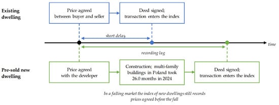
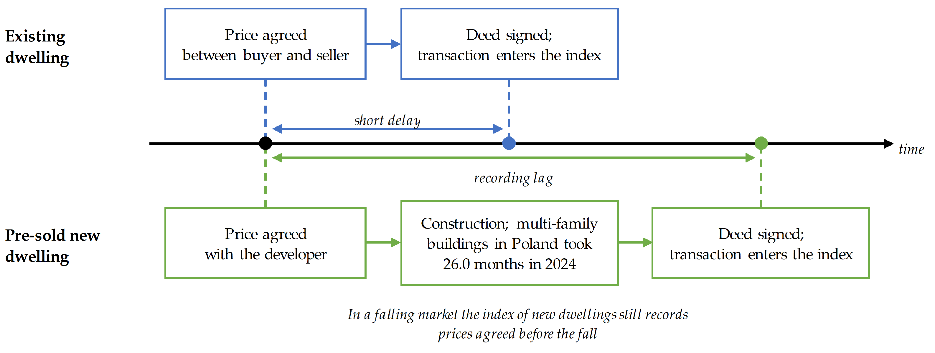
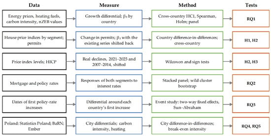
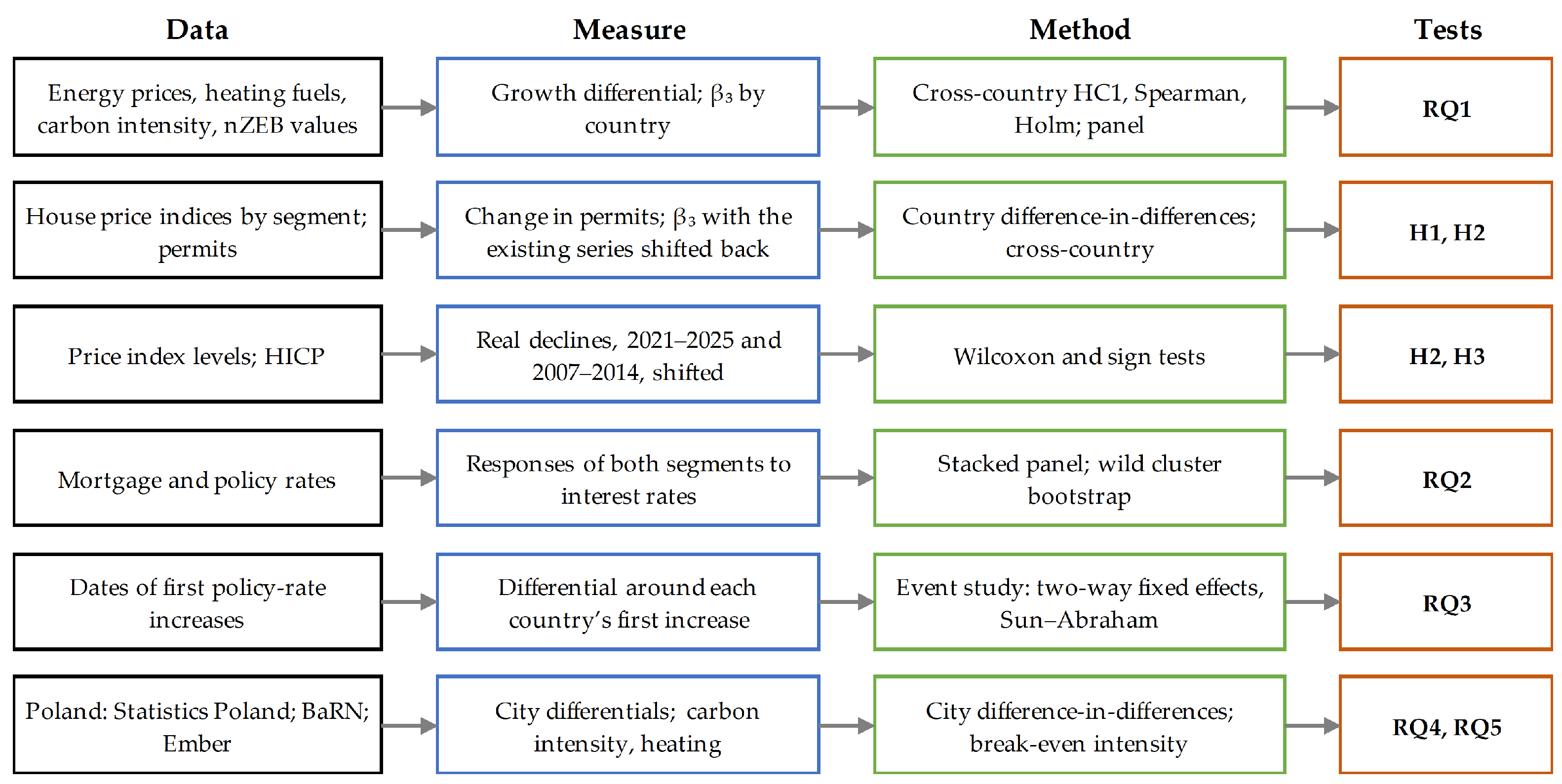
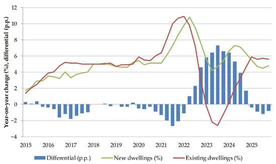
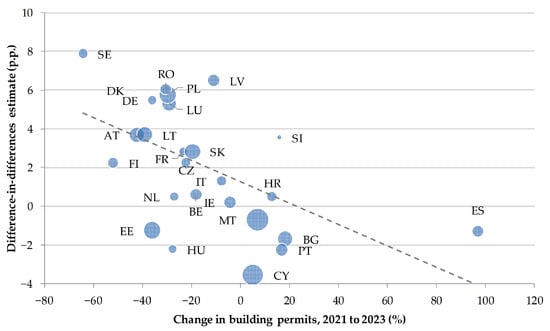
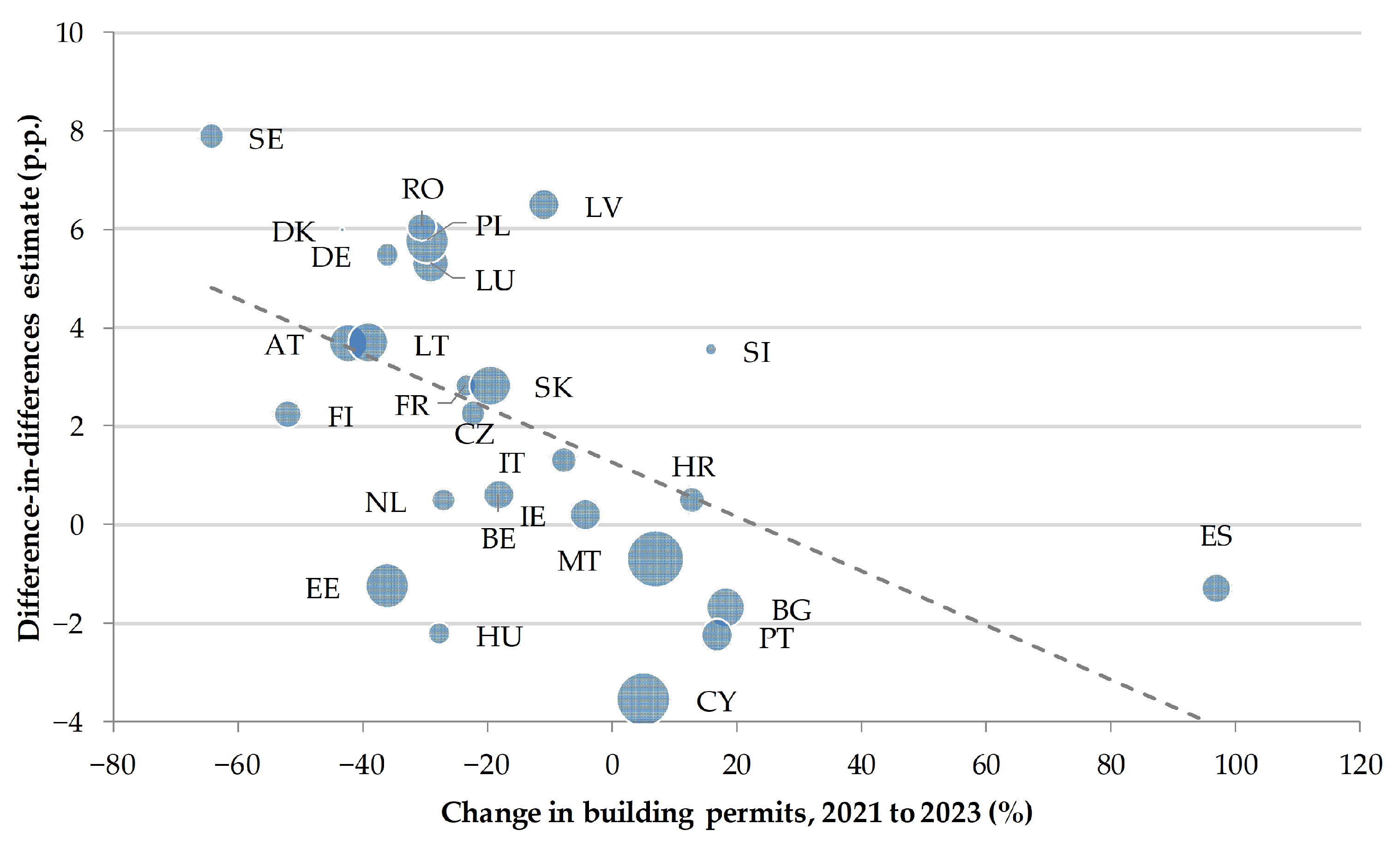
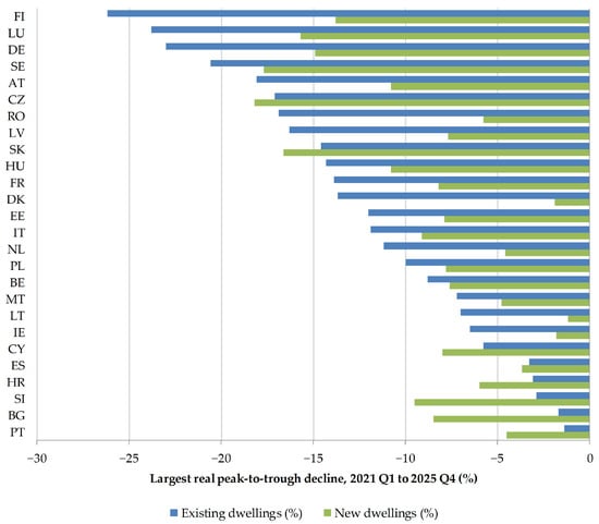
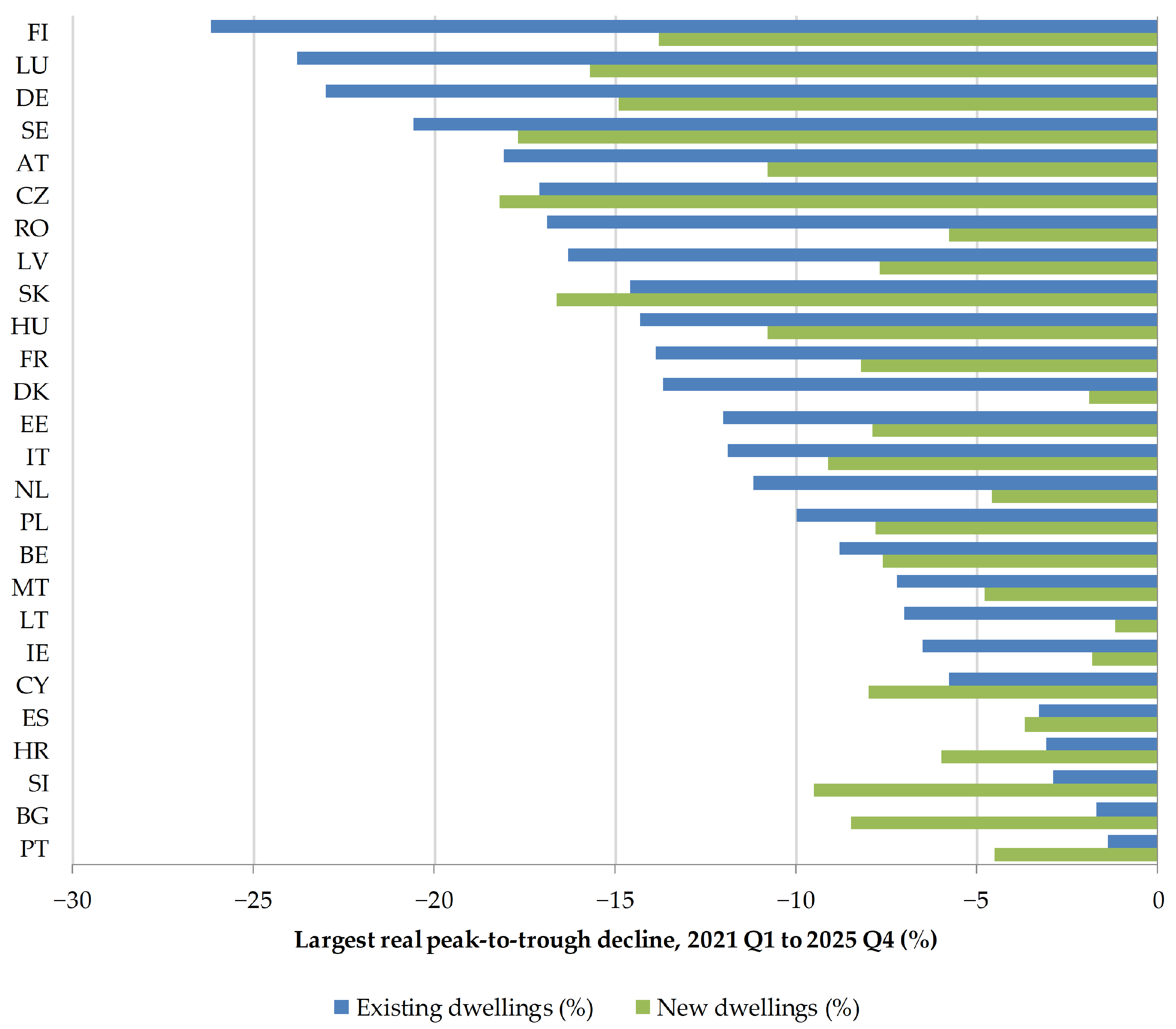
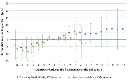
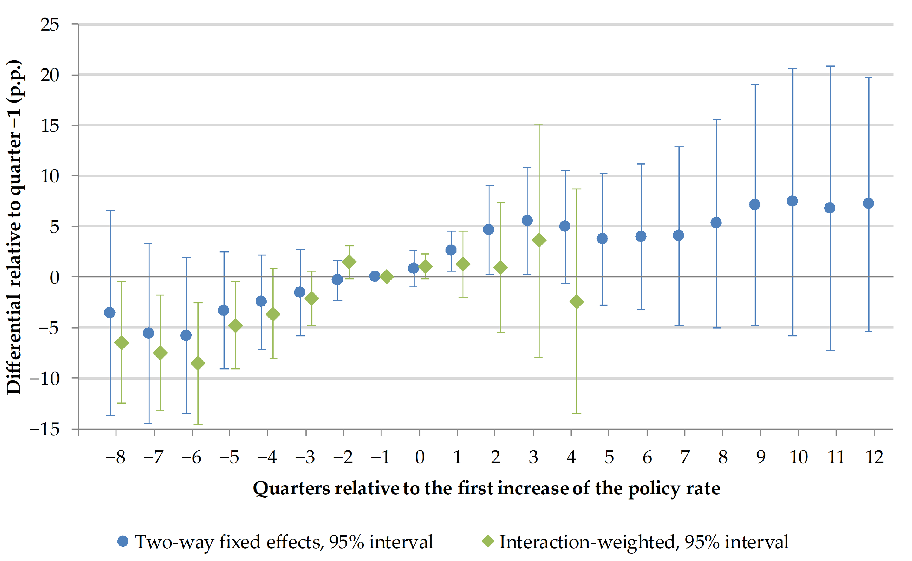
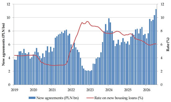
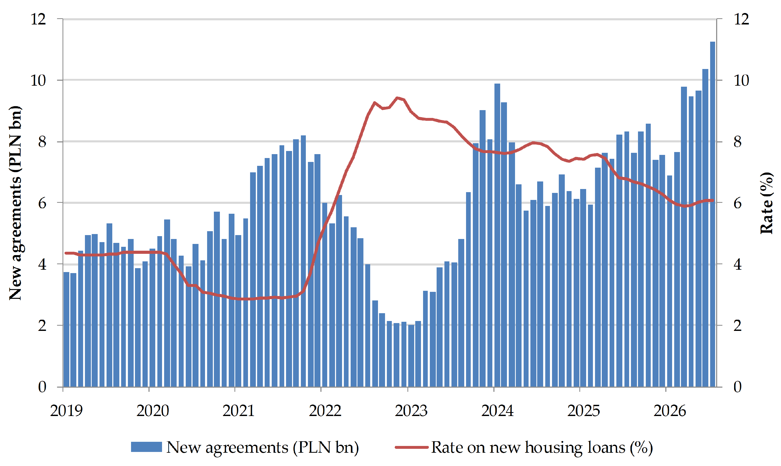
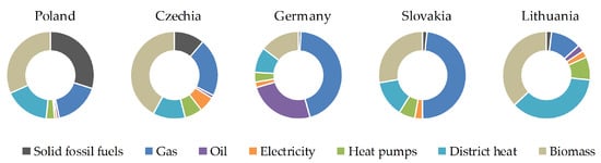
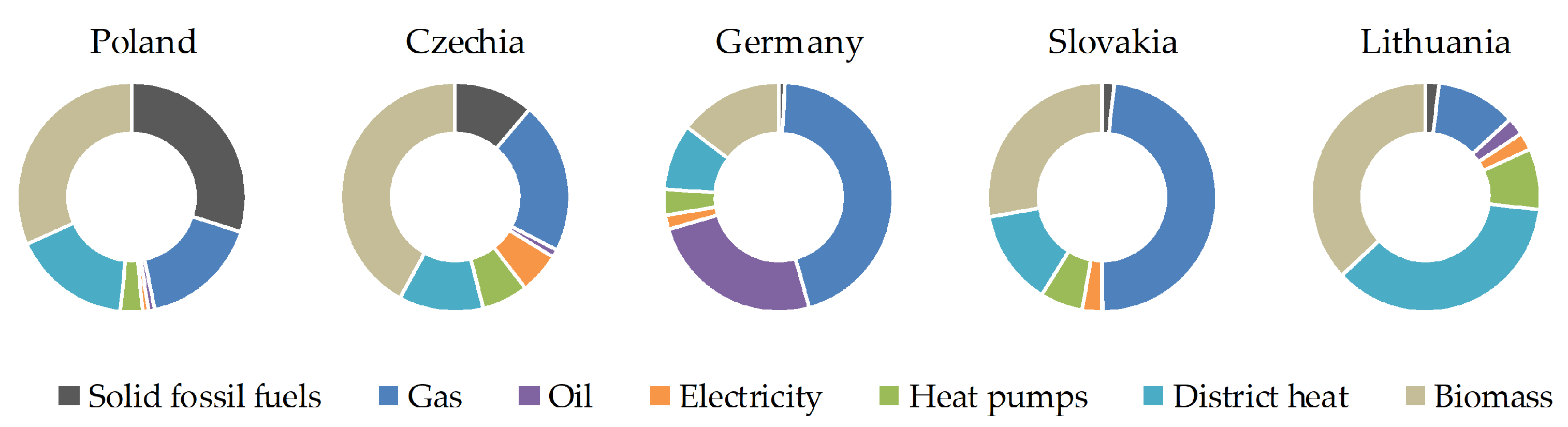

Disclaimer/Publisher’s Note: The statements, opinions and data contained in all publications are solely those of the individual author(s) and contributor(s) and not of MDPI and/or the editor(s). MDPI and/or the editor(s) disclaim responsibility for any injury to people or property resulting from any ideas, methods, instructions or products referred to in the content. |
© 2026 by the authors. Licensee MDPI, Basel, Switzerland. This article is an open access article distributed under the terms and conditions of the Creative Commons Attribution (CC BY) license.