


Abstract
Techno-economic optimization of residential photovoltaic (PV) systems often yields continuous capacities that are not directly buildable. This study develops an integrated framework linking techno-economic sizing, discrete component selection, rooftop geometry, low-voltage grid interconnection, and screening-level decarbonization. Three residential targets previously obtained with HOMER Pro (0.460, 1.310, and 3.890 kW) at 4.45 MXN/kWh were translated into commercial configurations. Evaluation of 430–460 W modules and compatible microinverters selected a 435 W module and IQ8A architecture, producing 1-, 3-, and 9-module systems of 0.435, 1.305, and 3.915 kWp with a mean absolute sizing deviation of 2.15%. At a 16° tilt, the minimum inter-row spacing was 0.817 m, with reserved rooftop areas of 6.754, 13.433, and 36.770 m2. Hourly PVGIS-ERA5 simulations (2019–2023), accounting for temperature, electrical losses, inter-row shading, and microinverter clipping, yielded mean annual AC generation of 855.32, 2565.95, and 7688.61 kWh, respectively. The corresponding annual clipping losses were 4.50, 13.50, and 40.51 kWh. Using the official 2024 Mexican grid emission factor of 0.444 tCO2e/MWh, the estimated avoided operational emissions were 0.380, 1.139, and 3.414 tCO2e/year, respectively. The framework links optimization to implementable residential PV designs, complemented by independent economic screening and illustrative point-of-connection voltage-rise analysis, both subject to site-specific validation.
1. Introduction
The transition toward low-carbon energy systems is reshaping the global electricity-generation landscape. In 2025, IRENA reported approximately 692 GW of net renewable capacity additions, of which about 511 GW corresponded to solar capacity [1]. Complementarily, the IEA Photovoltaic Power Systems Programme estimated nearly 698 GW of new PV installations during the same year and global cumulative PV capacity approaching 3 TW [2]. The difference between these figures reflects different scopes and accounting methodologies; therefore, they are used here solely to contextualize the scale of recent expansion. These trends confirm that PV technology is a central clean-energy option for electricity-sector decarbonization.
Within this expansion, distributed PV generation occupies a strategic position because it produces electricity close to the point of consumption. The International Energy Agency estimates that distributed solar applications, including residential, commercial, industrial, and off-grid systems, will account for approximately 42% of the projected PV expansion between 2025 and 2030, driven mainly by declining technology costs, retail electricity prices, self-consumption, and supporting policies [3]. Likewise, the IEA PVPS reports that distributed markets serving users who consume electricity while also producing part of the energy they use continue to expand and that, although centralized installations retain a majority share, distributed applications represent a structurally significant fraction of the global PV market [4].
Beyond installed-capacity growth, the climate value of distributed PV depends on how much grid electricity can be displaced by systems that are actually deployable. Clean-energy planning therefore requires not only identifying economically attractive capacities but also translating them into discrete systems whose spatial, electrical, and decarbonization performance can be quantified. At the same study location, previous work reported 281,175 kWh/year of PV generation from 173 kW of installed capacity and estimated 121.6 tCO2/year of avoided operational emissions using a national grid emission factor of 0.000433 tCO2/kWh [5]. These values provide a site-consistent reference for linking implementable residential PV design with a first-order decarbonization assessment.
Recent studies reinforce the role of rooftop and distributed PV as a practical decarbonization pathway once spatial and implementation constraints are explicitly represented. At national scale, Zhang et al. quantified rooftop-PV carbon-mitigation potential and showed that the benefit depends jointly on rooftop availability, solar resource, and grid-emission intensity [6]. At urban and building scales, Rayegan et al. [7] reported that large-scale rooftop PV deployment could reduce operational CO2 emissions and increase local energy self-sufficiency, while Zhang et al. [8] demonstrated the combined technical, economic, spatial, and environmental potential of community-level distributed PV systems. For residential rooftop retrofits, Yao et al. further showed that carbon and economic objectives can be treated jointly as design criteria [9]. These findings support coupling implementable rooftop design with explicit carbon-related indicators rather than reporting nominal PV capacity alone.
At the same time, avoided operational emissions should not be conflated with full life-cycle carbon performance. IEA PVPS emphasizes that PV life-cycle assessment includes manufacturing, installation, operation, and end-of-life stages and that manufacturing remains a major contributor to the environmental footprint of PV electricity [10]. Recent review evidence likewise identifies manufacturing as a principal environmental hotspot and shows that results are sensitive to technology, production scale, and life-cycle assessment assumptions [11]. For Mexico, SEMARNAT established the 2024 emission factor of the National Electric System at 0.444 tCO2e/MWh for indirect electricity-emission accounting [12], while the CNE documents its evolution from 0.582 tCO2e/MWh in 2017 to 0.444 tCO2e/MWh in 2024 [13]. Accordingly, the present study uses the official 2024 factor for operational grid displacement and treats this indicator separately from life-cycle emissions.
Residential rooftop PV systems are one of the most important expressions of distributed generation because they use already-built surfaces, reduce the need for additional land, and directly link generation with end-user consumption. However, the actual potential of a rooftop PV installation does not depend solely on the available irradiation. Climate, building characteristics, the fraction of usable roof area, orientation, array geometry, shading losses, demand profile, and grid interaction can significantly affect performance [14]. Residential-scale studies have also shown that housing typologies and effectively available surface area can produce substantial differences in self-consumption potential and installable PV capacity [15].
These conditions turn residential PV sizing into a design problem involving energy, economic, and spatial constraints simultaneously. Ioannou et al. [16] showed that, on flat residential roofs, row geometry, module dimensions, and self-shading losses affect the optimal design, and that maximizing energy production does not necessarily lead to the same solution as maximizing economic profitability. Therefore, a given nominal capacity is not, by itself, a sufficient design specification; it must be translated into a physical configuration compatible with the actual dimensions and constraints of the roof.
A substantial share of the research on residential PV systems has focused on techno-economic assessment. Fuster-Palop et al. [17], through the analysis of urban buildings, identified shading losses and unit power cost as variables particularly relevant to the payback period of PV installations. Garabitos Lara et al. [18] showed that residential consumption level and tariff rules can significantly modify system profitability and the economically favorable system size. These findings demonstrate that the economically convenient size of a PV system depends on both demand behavior and the economic conditions under which it operates.
Tariff structure is, in particular, one of the most influential factors in residential investment decisions. Cai et al. [19] developed a techno-economic framework that incorporated different electricity-pricing mechanisms, storage, and demand response, concluding that the tariff mechanism is one of the main determinants of the economic benefits of residential PV. Recent studies of urban PV integration have also used indicators such as life-cycle cost, levelized cost of electricity, payback period, and benefit-to-cost ratio to quantify energy performance and profitability simultaneously [20]. Similarly, comparative analyses of conventional rooftop PV and building-integrated solutions show that integration-architecture decisions can modify the levelized cost of energy, electricity generation, and avoided emissions [21].
Nevertheless, determining an economically optimal capacity is only one part of the design process. Once the target power is defined, it must be translated into an integer number of modules, a geometric configuration, and physically available roof area. Radwan et al. [22] evaluated the combined effects of tilt, module spacing, height, and albedo on the annual output of a residential PV system, showing that several of these variables have statistically significant effects on generated energy. In this context, inter-row spacing is particularly important because it creates a trade-off between reducing shading losses and making efficient use of the available surface area [23].
The spatial-layout problem has also been addressed using optimization models. Ma et al. [24] developed expressions to quantify the combined effects of tilt angle, spacing, and inter-row shading, showing that geometric configuration can significantly modify energy utilization per unit area. More recently, Hu [25] proposed an optimization framework specifically for rooftop PV systems, treating tilt angle, inter-row spacing, and string size as simultaneous design variables. The study showed that optimizing these parameters can increase energy generation and overall system efficiency.
Available surface area is another parameter that must be analyzed. It is a more complex constraint than the total geometric area of a roof.
In a review of 203 studies, Tian et al. [26] found that rooftop suitability for PV deployment depended on building constraints, layout criteria, regulatory conditions, and specific space-use requirements. Consequently, the physically existing roof area and the area that can actually be used for PV generation should not be considered equivalent. This distinction is especially relevant in residential applications, where access, inter-row spacing, obstacles, maintenance, safety, and the location of other equipment must be considered.
Alongside economic and geometric constraints, interaction with the electrical grid introduces a third dimension to the problem. The hosting-capacity literature has shown that increasing penetration of distributed PV generation can cause voltage rise, imbalance, overloading, and other operating-limit violations in low-voltage networks [27]. Assessments conducted on actual residential networks further confirm that hosting-capacity estimates depend on the assumed PV-system size and on geometric characteristics such as roof orientation and tilt [28]. These findings indicate that residential PV sizing should not be assessed exclusively from the user perspective; its interface with the distribution infrastructure must also be considered.
The relevance of this interaction becomes even clearer when operating constraints are incorporated. Jamroen et al. [29] showed that accounting for overvoltage-induced generation curtailment can significantly reduce the PV size considered optimal relative to an analysis that ignores this constraint, together with a reduction in profitability. This result indicates that a system that is economically attractive under a purely energy-based model may not remain the same solution once technical interconnection constraints are incorporated. Consequently, the inverter, protection devices, disconnection means, metering, and point of connection should be considered part of the system architecture from the design stage.
In Mexico, this consideration is particularly relevant because grid-connected residential PV installations fall within the distributed-generation scheme and must satisfy specific technical criteria. CFE Specification G0100-04 [30] defines the elements that comprise a PV generator, including modules, subarrays, connection boxes, cables, protection devices, grounding systems, and mounting structures, and it considers both grounded and ungrounded (floating) PV-generator electrical configurations. It also defines the inverter as the central element of the interface between the PV generator and the grid, responsible for converting direct current into synchronized alternating current and for performing additional protection and control functions.
The Manual for the Interconnection of Power Plants with Capacity below 0.5 MW establishes connection schemes, metering, protection requirements, and procedures associated with interconnection to the General Distribution Networks [31]. Among other provisions, it considers schemes for low-voltage installations with load centers and requires generation equipment to include protection against overcurrent, overvoltage, undervoltage, frequency variations, and islanding operation [31]. The National Energy Commission maintains the associated regulatory instruments within its distributed-generation documentation [32]. In this study, these documents provide the technical reference framework for translating the sized PV system into a residential electrical architecture suitable for interconnection.
Within the Mexican context, previous research has confirmed the technical, economic, and environmental potential of grid-connected PV systems under conditions of high solar availability. Acosta-Banda et al. [5] evaluated a grid-connected PV system in southeastern Mexico using HOMER Pro and demonstrated the feasibility of using solar generation to partially displace grid electricity while quantifying energy, economic, and environmental indicators. That study reported a site-specific annual PV yield and an operational grid-emission reference, thereby providing a consistent local basis for the decarbonization screening incorporated in the present framework.
Subsequently, Acosta-Banda et al. [33] specifically analyzed grid-connected residential systems using three demand profiles and different electricity purchase prices. The results showed that the economically selected configuration shifts from grid-only supply to PV/Converter/Grid as the purchase price increases, and that the optimal PV capacity also varies with demand and tariff conditions. At 5.00 MXN/kWh, for example, the selected PV capacities were 0.670, 1.790, and 4.840 kW for the three residential profiles analyzed. This previous work provides a quantitative basis for determining when and at what scale residential PV generation becomes economically attractive.
However, considering these studies together reveals an important methodological separation. On the one hand, numerous studies determine optimal PV capacity from energy variables, tariffs, and financial indicators [17,18,19,20,21,33]. On the other hand, geometric-design studies optimize tilt, spacing, shading, and rooftop utilization [16,22,23,24,25,26], while a third research line examines interconnection requirements and low-voltage network constraints [27,28,29,30,31,32]. Frameworks that directly connect these levels and translate a continuous capacity obtained through techno-economic optimization into a physically realizable residential installation are comparatively scarce. Such an installation must be defined by an integer number of commercial modules, actual rooftop area, mounting geometry, electrical configuration, protection devices, and an interconnection scheme. A further gap is that environmental benefits are commonly reported for optimized or nominal capacities before these discrete implementation constraints are propagated into the analysis. Consequently, the carbon-displacement potential associated with a continuous optimum may not correspond exactly to the physically installable system. This separation limits the direct transformation of simulation outputs into concrete design, implementation, and decarbonization decisions.
Compared with previous Mexican PV studies [5,33] and related techno-economic research [17,18,19,20,21], the present framework does not seek to establish a new continuous optimal capacity; instead, it translates previously optimized capacities into physically implementable configurations using integer numbers of commercial PV modules and compatible microinverters. While earlier studies have examined rooftop geometry, tilt, inter-row spacing, shading, and usable surface area [16,22,23,24,25,26], the specific contribution of this work is to connect these design considerations with discrete capacity selection, electrical compatibility, interconnection screening, configuration-specific AC electricity generation, and operational carbon-displacement indicators within a sequential methodology. Regarding structural feasibility, the assessment is limited to preliminary module-mass and average-pressure estimates and does not constitute verification of the load-bearing capacity of an individual roof. Site-specific structural calculations, wind-uplift assessment, measured operational validation, and detailed distribution-network studies therefore remain necessary before actual implementation. These distinctions define both the methodological contribution and the practical limitations of the proposed framework.
Therefore, the objective of this study is to develop and evaluate an integrated framework for grid-connected residential PV systems that combines techno-economic sizing, discrete module selection, rooftop-array geometry, electrical interconnection, and a screening-level decarbonization assessment. The purpose is to transform optimal simulation capacities into physically implementable low-carbon residential solutions and to quantify how discrete design decisions affect annual clean-energy contribution and operational CO2 displacement. The proposed framework links demand and economic conditions with module count, installable PV capacity, required rooftop area, array tilt and spacing, inverter capacity, the arrangement of protection, metering, and interconnection components, and post-design decarbonization indicators. In this way, the study moves beyond identification of an economically optimal capacity toward an integrated methodology for design, implementation, grid compatibility, and clean-energy decision-making.
2. Materials and Methods
2.1. General Methodological Framework
The study was structured around a sequential design framework linking three design levels: techno-economic sizing, physical translation of the optimal size, and electrical grid integration, followed by a screening-level clean-energy and decarbonization assessment. The methodological approach builds on the optimization previously performed with HOMER Pro [33,34], using the optimal capacities as design targets and determining how those continuous values can be converted into physically realizable residential configurations before their energy and operational carbon-displacement implications are quantified. This sequential workflow highlights the feasibility gate through which the discrete configuration must satisfy geometric, electrical, and interconnection requirements before the post-feasibility clean-energy and decarbonization assessment is performed.
The methodological workflow was organized into five design stages and one final implementable design output, as summarized in Figure 1. The stages were: (1) definition of solar-resource conditions, residential demand, and the reference economic condition; (2) adoption of the continuous capacities previously obtained with HOMER Pro as sizing targets; (3) translation of those capacities into discrete configurations through module and conversion-equipment selection; (4) development of the rooftop geometric design, including tilt, projection, self-shading, inter-row spacing, required area, and mass; and (5) definition of the electrical and interconnection architecture. After the geometric, electrical, and regulatory feasibility assessment, the final discrete configurations undergo a sixth analytical stage involving configuration-specific hourly photovoltaic simulations to estimate annual AC electricity generation, the PV-to-load energy ratio, potential avoided operational CO2e emissions, and avoided CO2e per unit of reserved rooftop area.
Figure 1.
Integrated methodological framework for translating techno-economic PV sizing into an implementable residential rooftop system.
The methodology was formulated so that electrical and geometric constraints act as feasibility conditions rather than as subsequent corrections. Thus, a simulation-derived solution is considered implementable only when it can be expressed using discrete commercial components, accommodated within a rooftop area compatible with its layout, and made to satisfy electrical interconnection requirements.
The clean-energy and decarbonization assessment is intentionally applied only after feasibility verification so that the simulated energy and emission indicators are attributed to the implementable discrete configuration rather than to the continuous optimization target.
2.2. Study Conditions and Design Input Data
2.2.1. Location and Solar Resource
The study was conducted in Santo Domingo Tehuantepec, Oaxaca, southern Mexico. The reference meteorological location was established at Universidad del Istmo, Campus Tehuantepec (16.288° N, 95.241° W), at an estimated elevation of 44 m above sea level, according to PVGIS geographical data. The location is used as a case study for applying the proposed framework. Historical data integrated into HOMER Pro indicate monthly mean global horizontal irradiation ranging from approximately 4.48 to 6.54 kWh/m2/day. April exhibits the highest monthly mean value, whereas November exhibits the lowest. The mean monthly temperature at the site is approximately 26.3 °C [33]. For the configuration-specific photovoltaic simulations, hourly meteorological data were obtained from the PVGIS-ERA5 database for the period 2019–2023, considering the study location (16.288° N, 95.241° W). The dataset includes direct, diffuse, and reflected solar irradiance on a south-facing surface tilted at 16°, ambient temperature, and wind speed. These data represent modeled meteorological conditions rather than on-site measurements.
2.2.2. Residential Demand Profiles
Three previously defined residential profiles [33] were used because they enable analysis of the physical scalability of the design (Table 1). The three residential demand profiles were adopted from the preceding HOMER Pro techno-economic study [33] and correspond to daily electricity requirements of 11.26, 30.00, and 83.30 kWh/day, representing low-, medium-, and high-demand residential scenarios, respectively. The hourly load series retained in the HOMER Pro source model are synthetic demand profiles used for scenario-based simulation rather than a statistically representative sample of measured household electricity consumption. Consequently, these profiles are employed to examine how the proposed design framework responds to increasing electricity demand and photovoltaic system size. The results should therefore be interpreted as representative of the selected demand scenarios rather than of the entire residential building stock in the study region.
Table 1.
Residential demand profiles used as design scenarios.
2.2.3. Reference Techno-Economic Condition
The previous analysis included ten electricity purchase prices, expressed through Equation (1). The results show that profiles D2 and D3 begin to adopt a PV/Converter/Grid configuration at 4.25 MXN/kWh, whereas D1 does so at a higher price [33].
The electricity purchase price of 4.45 MXN/kWh was selected as a common reference scenario based on the tariff-sensitivity analysis conducted in the preceding HOMER Pro study [33] and documented in Supplementary Material S1. Its significance lies in providing an economic condition under which all three residential demand profiles select a PV/Converter/Grid architecture, allowing their continuous optimal capacities to be compared and subsequently translated into physically implementable configurations. The tariff is therefore employed as a consistent analytical reference rather than as a universally applicable CFE electricity rate or a general threshold for photovoltaic adoption. At lower electricity purchase prices, the economic preference for photovoltaic generation varies among the demand profiles, as demonstrated by the sensitivity analysis. The corresponding continuous optimal capacities at the selected reference tariff are presented in Table 2.
Table 2.
Continuous techno-economic capacities used as design targets at 4.45 MXN/kWh [33].
2.3. Translation from Continuous Design to Discrete Configurations
A PV capacity obtained through optimization may take any continuous value, whereas an actual installation requires an integer number of modules. This difference was addressed as a discrete selection problem. For each target capacity, the implementable power is expressed by Equation (2), where Ni is an integer number of modules and Pm is the rated power of a commercial module.
For each candidate module rating, the number of units was determined using Equation (3).
The relative deviation from the continuous optimum was calculated as:
To avoid selecting a module that performs well for only one profile while producing large deviations for the others, the mean absolute deviation was defined as:
The module was selected by minimizing Equation (6), where P denotes the set of commercial module ratings evaluated.
2.4. Evaluation of Commercial PV Modules
To prevent geometric differences among manufacturers from simultaneously affecting the selection process, the residential Trina Solar Vertex S+ TSM-NEG9R.28 series (Trina Solar Co., Ltd., Changzhou, Jiangsu, China) was used as the reference family. This series is available in power classes from 430 to 460 W. All modules in the series share the same external dimensions of 1762 × 1134 × 30 mm and an approximate mass of 21.0 kg, allowing the effect of rated power to be analyzed without changing the physical area of each unit [35]. The evaluated power classes are listed in Table 3.
Table 3.
Commercial components evaluated during the discrete design stage.
The set of evaluated module ratings, expressed in Wp, is given by Equation (7).
The geometric area of one module is obtained from:
2.5. Module-Level Microinverter Selection
The low capacity of scenario D1 makes it impractical to impose a string-inverter architecture because a single PV module may not satisfy the minimum MPPT voltage of a conventional inverter. Therefore, an architecture based on module-level power electronics (MLPE) was adopted, and microinverters from the Enphase IQ8 family were evaluated [36]. Selection was performed after determining module power and simultaneously considered the voltage, current, and power-compatibility constraints given in Equations (10a)–(10c). To maintain a common electrical condition for D1, D2, and D3, the reference implementation was defined for a single-phase, three-wire 120/240 V, 60 Hz residential service, one of the domestic voltage configurations considered by CFE [30].
The installed AC capacity is calculated as:
The deviation from the converter capacity previously obtained with HOMER Pro is expressed as:
As with the PV array, the following comparative criterion was used:
The PV-to-inverter sizing ratio is defined as [37]:
This parameter was used as a design indicator rather than as a universal value imposed a priori because the literature shows that an appropriate value depends on site conditions, irradiance, temperature, inverter clipping, and equipment-specific characteristics [37].
2.6. Rooftop Geometric Design
2.6.1. Roof Type, Orientation, and Tilt
The system was designed for a reference residence with a flat concrete roof. CFE Specification G0100-04 recommends orienting the PV generator toward the south and using a tilt approximately equal to the geographic latitude while also accounting for building constraints. It also indicates that module shading, even partial shading, should be avoided [30]. At a latitude of φ ≈ 16.28°, a constructive tilt of β = 16° was adopted. This tilt is consistent with the site latitude and facilitates geometric interpretation of the design without introducing discrepancies between the orientation criterion and the technical representation of the array.
2.6.2. Module Height and Horizontal Projection
For a module installed in portrait orientation, the height difference between its edges and its horizontal projection were determined using Equations (15)–(18). For Lm = 1.762 m and β = 16°, the resulting values were h ≈ 0.486 m and Lp ≈ 1.694 m. These are the geometric dimensions used in Figure 2 and in the subsequent spacing and required-area calculations.
Figure 2.
Solar-geometric basis for module tilt and inter-row spacing on a flat residential roof.
2.7. Inter-Row Shading Criterion
Inter-row spacing was determined using solar geometry [38]. Solar declination, hour angle, and solar elevation were calculated using Equations (19)–(21).
The winter solstice was adopted as a conservative design condition, and mutual row shading was avoided approximately over the 09:00–15:00 solar-time interval. For φ = 16.28°, the critical solar elevation at 09:00 on the winter solstice was αcrit ≈ 30.74°. The required minimum spacing was calculated using Equation (22). With β = 16°, the module geometry yields Dmin ≈ 0.817 m. This calculation uses the full horizontal shadow length and therefore establishes a conservative criterion for row-normal spacing because it does not reduce the shadow length through azimuthal projection.
Consequently, an inter-row spacing of = 0.82 m, slightly greater than the calculated minimum value, was adopted for the geometric model. The corresponding row pitch was calculated using Equation (24), yielding Pr ≈ 2.514 m. In a detailed engineering design, the final spacing should incorporate mounting tolerances and the specific conditions of the roof.
2.8. Area and Rooftop Layout Indicators
The net PV area, geometric width, array depth, and minimum geometric footprint were calculated using Equations (25)–(28).
To represent the area required for inspection and maintenance, a service margin of M = 0.60 m was included as a uniform design assumption for all three scenarios rather than as a minimum distance prescribed by CFE. The reserved rooftop area and surface-utilization ratio were calculated using Equations (29) and (30).
The CFE specification recognizes that the required surface area depends on installed capacity and module dimensions, and it also indicates the convenience of providing accessible and protected areas for electrical equipment [30].
2.9. Preliminary Structural Assessment
The proposed design corresponds to a geometric and electrical integration level. A preliminary assessment of the additional mass introduced by the modules was also incorporated using Equations (31) and (32).
The mass and pressure obtained from these expressions do not include the aluminum support structure, anchors, ballast, conduits, or wind loads. Final sizing of anchors, profiles, slab capacity, and uplift resistance must be based on a residence-specific structural calculation that accounts for the particular building characteristics.
2.10. Electrical Architecture and Grid Interconnection
2.10.1. Reference Regulatory Configuration
The reference electrical configuration was taken from CFE Specification G0100-04, corresponding to the electrical configuration of the ungrounded (floating) PV generator [30]. The specification recognizes two general PV-generator configurations: grounded and ungrounded (floating). For the ungrounded configuration, the array DC circuit operates without an intentional direct connection to ground. The diagram provided in CFE G0100-04 was used as a functional reference, and interpretation of the scheme was complemented with the Interconnection Manual, NOM-001-SEDE-2012, and current distributed-generation documentation [31,32,39].
2.10.2. Adaptation to a Module-Level Conversion Architecture
Because of the small size of the residential scenarios, particularly D1, the proposed design uses module-level conversion through microinverters. NOM-001-SEDE-2012 addresses AC modules in Article 690-6 [39]. For the reference electrical case, a 120/240 V, 60 Hz interface was considered, consistent with the nominal voltage of the selected IQ8A and with one of the domestic configurations indicated by CFE [30,36]. Accordingly, the proposed functional architecture is expressed by Equation (33). Residences with a different voltage or number of phases require selection of a compatible microinverter and repetition of the electrical verification described in Section 2.5.
Individual conversion avoids the need to form high-voltage DC strings and allows the same modular architecture to be used for D1, D2, and D3.
2.10.3. Metering and Disconnection
The Manual for the Interconnection of Power Plants with Capacity below 0.5 MW establishes that Interconnection Scheme 1 may be used for low-voltage generating facilities supplying load centers, in which billing meter MF records both energy received from the grid and energy injected into it [31]. This configuration is consistent with the present study, in which the residence remains grid-connected and economic compensation for exported energy is not included in the techno-economic model. The scheme includes PV modules, microinverters, an AC branch circuit, overcurrent protection, generation disconnect I1, a residential load center, main service disconnect I2, bidirectional billing meter MF, equipment grounding, and connection to the distribution grid. CFE requires disconnection means, and the Manual specifies protection against overcurrent, overvoltage, undervoltage, frequency variations, and islanding operation [30,31]. The reference functional structure is shown in Figure 3a, whereas the proposed interconnection configuration is shown in Figure 3b.
Figure 3.
Electrical architecture of the proposed residential PV system and its interface with the CFE low-voltage grid: (a) functional reference based on CFE’s ungrounded (floating) PV-generator concept; and (b) proposed module-level conversion and interconnection scheme.
2.10.4. Point-of-Common-Coupling Voltage-Rise Screening
A deterministic, first-order voltage-rise screening was carried out at the point of common coupling (PCC) to complement the functional interconnection architecture. The calculation considers the 120/240 V, 60 Hz reference residential service described in Section 2.10.2 and the rated AC output of the final configurations. The upstream distribution system and service connection were represented by an equivalent line-to-line loop impedance, Zeq = Req + jX_eq, which referred to the 240 V interface. For a radial equivalent, the approximate voltage rise associated with net active and reactive power injection is ΔV ≈ (Req Pinj + Xeq Qinj)/Vnom [27,28,29,40,41,42]. With the microinverters operating at the assumed unity power factor (Qinj = 0), the expression reduces to ΔV ≈ Req Pinj/Vnom.
A conservative low-demand screening condition was adopted by setting the net export equal to the maximum AC rating of each configuration: Pinj = 0.349, 1.047, and 3.141 kW for D1, D2, and D3, respectively. Because measured feeder impedance, service-conductor data, and PCC voltage records were unavailable, the equivalent loop resistance was varied parametrically across illustrative values of 0.10, 0.30, and 0.50 Ω. These assumed values are sensitivity scenarios, not measured characteristics of the local distribution network.
An illustrative pre-generation PCC voltage of V0 = 1.03 p.u. (247.2 V) and an upper screening level of Vlim = 1.05 p.u. (252.0 V), both referred to 240 V, were considered to examine the remaining voltage headroom. The screening condition was V0 + ΔV ≤ Vlim, with a corresponding voltage-limited local injection threshold Pmax ≈ (Vlim − V0)Vnom/Req. These operating points provide a transparent stress test rather than a determination of the applicable utility acceptance criteria, feeder-wide PV hosting capacity, or compliance with all interconnection requirements.
2.11. Equipment Location in the Residence
The microinverters are installed beneath the PV modules themselves; therefore, an exterior-wall area equivalent to that required for a central inverter does not need to be reserved. The technical wall area should primarily contain the AC combination/protection enclosure, generation disconnect I1, service disconnect I2 according to the building configuration, meter MF, and the conduit and grounding routes. The CFE specification recommends that, where applicable, power-conditioning and disconnecting equipment be located on a shaded and protected wall [30]. Universal dimensions were not assigned to the meter or protection enclosure because these depend on the authorized equipment and the specific conditions of the service connection.
2.12. Design Performance Indicators
The configurations were compared using five groups of indicators. Agreement with continuous sizing was quantified using |εPV| and |εAC|; physical rooftop utilization using APV, Afoot, Areq, and ηA; and electrical adequacy using RDC/AC together with compatibility in voltage, current, frequency, and interconnection requirements. A fourth group addresses economic performance through two complementary assessments. The NPC, LCOE, ROI, and payback-period indicators previously obtained from the continuous HOMER Pro optimization [33] are retained as reference values. The final discrete configurations are evaluated separately using an independent cash-flow model, which estimates NPC, the levelized cost of total electricity supplied, average annual simple ROI, and simple payback period, as described in Section 2.16. Differences between these two sets of indicators are not attributed exclusively to capacity discretization because their meteorological inputs and calculation procedures are not identical. A fifth group evaluates clean-energy and decarbonization performance through configuration-specific simulated annual AC generation, the annual PV-to-load energy ratio, estimated potential avoided operational CO2e emissions, and avoided CO2e per unit of reserved rooftop area.
2.13. Feasibility Criterion
An implementable configuration was defined as one that simultaneously satisfies the geometric, electrical, and regulatory feasibility conditions given in Equations (34)–(38).
Among the feasible configurations, priority was given to the one that minimizes deviation from continuous sizing without introducing geometric or electrical incompatibilities. The selection process is hierarchical; therefore, no weighted index combining economics, surface area, and capacity through subjective weights was constructed.
2.14. Configuration-Specific Hourly PV Energy Simulation
The hourly photovoltaic simulation was defined for the three final residential configurations: D1, consisting of one 435 W module; D2, comprising three 435 W modules arranged in a single row; and D3, consisting of nine 435 W modules arranged in three rows of three modules each. All configurations were specified with a fixed tilt angle of 16° and a south-facing orientation (azimuth of 0°). For D3, an inter-row spacing of 0.82 m was adopted. Each photovoltaic module was paired with an Enphase IQ8A microinverter with a continuous AC power rating of 349 VA, resulting in total installed AC capacities of 0.349, 1.047, and 3.141 kW for D1, D2, and D3, respectively.
The hourly meteorological dataset obtained from PVGIS-ERA5 for 2019–2023 was used to characterize the solar resource and environmental conditions at the study location. The dataset provides three components of solar irradiance incident on the tilted photovoltaic surface: direct irradiance (Gb(i)), diffuse irradiance (Gd(i)), and ground-reflected irradiance (Gr(i)). Hourly ambient temperature (T2m) and wind speed at 10 m above ground level (WS10m) were also considered as inputs for estimating photovoltaic module operating temperature.
The total plane-of-array irradiance for each hourly interval was calculated as the sum of the direct, diffuse, and ground-reflected irradiance components provided by PVGIS, before applying the inter-row shading correction:
where represents the total plane-of-array irradiance at hour t (W/m2), while , , and represent the direct, diffuse, and ground-reflected irradiance components, respectively.
Inter-row shading was considered for configuration D3, which consists of three rows of photovoltaic modules. Configurations D1 and D2 contain only one row and therefore do not experience mutual inter-row shading. For D3, the shading assessment considers the hourly solar position, module dimensions, tilt angle of 16°, and the adopted inter-row spacing of 0.82 m. The resulting shading correction is applied to the direct irradiance component to account for potential reductions in photovoltaic generation.
The effective plane-of-array irradiance was expressed by applying an hourly inter-row shading factor to the direct irradiance component, while maintaining the diffuse and ground-reflected irradiance contributions, as follows:
where the superscript eff denotes effective irradiance and f_sh,t represents the hourly fraction of direct irradiance reduced by inter-row shading, ranging from 0 to 1. For D1 and D2, f_sh,t = 0 because both configurations consist of a single row. For D3, the shading factor depends on the hourly solar position and the geometric overlap of shadows between adjacent rows.
Hourly photovoltaic cell temperature was estimated using the Sandia Array Performance Model (SAPM), considering effective plane-of-array irradiance, ambient air temperature, and wind speed at 10 m above ground level. Given the glass–glass construction of the selected photovoltaic modules and their installation on inclined supports above a flat roof, an open-rack glass–glass thermal configuration was adopted as a modeling assumption. The resulting hourly cell temperature was used to account for temperature-dependent variations in DC power output.
The hourly module back-surface temperature was calculated using the Sandia thermal model, which relates incident solar irradiance, ambient temperature, and wind speed through empirical coefficients associated with the module construction and mounting configuration, as follows:
where represents the module back-surface temperature at hour t (°C), is the ambient air temperature (°C), denotes the effective plane-of-array irradiance (W/m2), and is the wind speed measured or estimated at a height of 10 m (m/s). The empirical coefficients = −3.47 and = −0.0594 s/m correspond to the open-rack glass–glass configuration of the Sandia Array Performance Model (SAPM). These reference values were adopted as modeling assumptions rather than as manufacturer-specific thermal measurements.
The hourly photovoltaic cell temperature was subsequently calculated from the module back-surface temperature by incorporating the temperature difference between the cells and the module surface, according to the Sandia thermal model, as follows:
where is the photovoltaic cell temperature at hour t (°C), is the module back-surface temperature (°C), is the effective plane-of-array irradiance (W/m2), and is the reference irradiance, set to 1000 W/m2. The parameter ΔT represents the temperature difference between the cells and the module back surface at the reference irradiance; a value of 3 °C was adopted for the open-rack glass–glass configuration of the Sandia Array Performance Model (SAPM).
The hourly DC power output was estimated using the rated power of the selected Trina Solar Vertex S+ TSM-NEG9R.28 photovoltaic modules, the effective plane-of-array irradiance, and the calculated cell temperature. Each module has a nominal power rating of 435 W under standard test conditions (STC) and a maximum-power temperature coefficient of −0.29%/°C, according to the manufacturer’s technical specifications. The model accounts for irradiance-dependent power generation and temperature-related efficiency variations.
The hourly DC power output of each photovoltaic module, before additional system losses, was calculated using the incident effective irradiance and the cell-temperature correction relative to standard test conditions, as follows:
where is the hourly DC power output of an individual photovoltaic module (W); = 435 W is its rated power under standard test conditions; denotes the effective plane-of-array irradiance (W/m2); = 1000 W/m2 is the reference irradiance; = −0.0029 °C−1 is the temperature coefficient of maximum power; denotes the photovoltaic cell temperature at hour t (°C); and = 25 °C is the reference cell temperature under standard test conditions. The calculated DC power refers to one module before additional non-temperature system losses and AC conversion.
The hourly DC power estimated using Equation (43) was subsequently adjusted to account for additional system losses, particularly soiling and DC-side electrical losses. These losses were represented by separate correction factors to avoid double counting the effects of irradiance, temperature, and inter-row shading already considered in the preceding equations. Consistent loss assumptions were applied to the three residential configurations to enable a comparable assessment of their energy performance. The loss factors were treated as modeling assumptions rather than site-specific measurements.
The net hourly DC power available at the microinverter input was calculated by applying separate correction factors for soiling and DC-side electrical losses, as expressed in Equation (44):
where is the net DC power available at the microinverter input at hour t (W); is the DC power calculated with Equation (43), before additional system losses (W); is the fractional loss caused by soiling; and is the fractional loss associated with DC-side electrical components and connections. Both loss factors are dimensionless and range from 0 to 1.
In the absence of site-specific measurements, soiling and DC-side electrical losses were each assumed to be 2% for the base-case simulation, using the default loss categories of the NREL PVWatts model as reference. These assumptions were applied consistently across the three configurations. Temperature effects, inter-row shading, and inverter conversion losses were modeled separately to avoid double counting.
The net DC power was converted into AC power considering the conversion efficiency and continuous output power limit of each Enphase IQ8A microinverter. A CEC-weighted efficiency of 97% was adopted as a constant-efficiency approximation, while the continuous AC output was limited to 349 W per microinverter, assuming unity power factor. The hourly AC power output was calculated as follows:
where is the hourly AC power delivered by an individual IQ8A microinverter (W); = 0.97 is the assumed constant DC-to-AC conversion efficiency, approximated from the manufacturer’s CEC-weighted efficiency; is the net DC power supplied to the microinverter at hour t (W), as calculated using Equation (44); and = 349 W is the maximum continuous AC output power of one IQ8A microinverter, assuming the unity power factor. The min operator selects the smaller of the unconstrained converted power and the microinverter power limit. Power clipping occurs when the unconstrained converted power exceeds 349 W. Equation (45) is applied independently to each module–microinverter pair.
To quantify inverter clipping losses, the hourly AC-equivalent power curtailed by each microinverter was calculated as the positive difference between the unconstrained converted power and the maximum continuous AC output capacity, as expressed in Equation (46):
where denotes the hourly AC-equivalent power curtailed by inverter clipping (W); is the assumed inverter conversion efficiency (0.97); is the net DC power available at the microinverter input (W); and is the maximum continuous AC output power of each Enphase IQ8A microinverter (349 W). The maximum operator ensures that clipping losses are zero whenever the unconstrained AC-equivalent power does not exceed the continuous output limit.
The annual AC energy generated by each final residential PV configuration was calculated by integrating the hourly AC power output of all module-level microinverters over each calendar year, as follows:
where is the annual AC energy generated by configuration in year (kWh/year); j denotes the residential configuration (D1, D2, or D3); is the number of PV modules and corresponding IQ8A microinverters (1, 3, or 9, respectively); PAC,m,t is the hourly AC power output of microinverter m at time (W), calculated using Equation (45); and =1 h is the simulation time step. The factor 1/1000 converts watt-hours into kilowatt-hours. Each calendar year from 2019 to 2023 was evaluated separately, including the additional day of 2020.
The annual energy curtailed by inverter clipping was determined by integrating the hourly AC-equivalent power losses of the module-level microinverters over each calendar year, as follows:
where represents the annual AC-equivalent energy lost due to inverter clipping in configuration j during year y (kWh/year); is the hourly curtailed AC-equivalent power of microinverter m at time t (W), calculated according to Equation (46); is the number of PV modules and corresponding microinverters in configuration j; and =1 h is the simulation time step. The factor 1/1000 converts watt-hours to kilowatt-hours.
2.15. Clean-Energy and Decarbonization Assessment
Following the geometric and electrical feasibility assessment, the final discrete photovoltaic configurations were evaluated using the hourly simulation methodology described in Section 2.14. Annual AC electricity generation was calculated for each configuration over the 2019–2023 period, and the five-year mean was used for comparative energy and decarbonization indicators. The previously reported specific yield of 1625.29 kWh/kWp/year for a 173 kW photovoltaic system [5] was retained exclusively as a reference benchmark rather than as an input for estimating the generation of the discrete configurations. Avoided operational emissions were estimated using the official 2024 Mexican grid emission factor of 0.000444 tCO2e/kWh [12,13], assuming one-for-one displacement of grid electricity by the simulated AC generation.
For each discrete configuration, annual AC electricity generation was obtained from the hourly simulations described in Section 2.14, using the mean annual output for 2019–2023. Annual residential electricity demand was calculated by multiplying daily demand by 365, and the PV-to-load energy ratio was determined by dividing the simulated annual AC generation by annual residential demand. Potential avoided operational CO2e emissions were estimated by multiplying annual AC generation by the official Mexican grid emission factor, assuming one-for-one displacement of grid electricity. The spatial carbon-displacement indicator was calculated by dividing the estimated avoided emissions by the reserved rooftop area. These indicators represent screening-level estimates and do not establish actual hourly self-consumption or grid displacement.
The resulting indicators represent simulation-based estimates of operational energy generation and potential carbon displacement rather than measured system performance or a comprehensive life-cycle assessment. Although the hourly model considers meteorological variability, module temperature, assumed soiling and electrical losses, inter-row shading, and inverter clipping, the assessment does not include measured system performance, annual module degradation, embodied emissions, equipment manufacturing, replacement, transportation, or end-of-life processes. Furthermore, the estimated avoided emissions assume that all generated AC electricity displaces grid electricity, without explicitly evaluating hourly coincidence between photovoltaic generation and residential demand. Consequently, these indicators should be interpreted as preliminary estimates of operational decarbonization potential under the adopted modeling assumptions.
2.16. Economic Re-Evaluation of the Final Discrete Configurations
The economic performance of the three physically implementable photovoltaic configurations was assessed using an independent discounted cash-flow model with fixed PV capacities of 0.435, 1.305, and 3.915 kWp and corresponding AC conversion capacities of 0.349, 1.047, and 3.141 kW. The configuration-specific hourly AC generation estimates described in Section 2.14 were combined with the synthetic residential demand profiles contained in the original HOMER Pro model [33] to estimate photovoltaic self-consumption, grid electricity purchases, and surplus generation.
The economic assessment retained the original financial assumptions, including a 25-year project horizon, a 12% nominal interest rate, 3.8% inflation, an electricity purchase price of 4.45 MXN/kWh, and zero remuneration for electricity exported to the grid. Initial investment, operation and maintenance costs, converter replacement, and residual value were considered using the generic component-cost assumptions from the original model. Consequently, the economic results represent a screening-level assessment of the final discrete configurations rather than a new HOMER Pro optimization or a quotation based on the commercial prices of the selected equipment.
The economic calculations adopted the generic component-cost assumptions contained in the original HOMER Pro model: 15,000 MXN/kWp for photovoltaic investment, 4000 MXN/kW for AC conversion equipment, and 5000 MXN/kWp/year for photovoltaic operation and maintenance. The converter lifetime was assumed to be 15 years, with replacement in year 15 and a proportional residual value credited at the end of the 25-year project horizon. The nominal interest rate of 12% and inflation rate of 3.8% correspond to a real discount rate of approximately 7.90%. Hourly photovoltaic self-consumption was estimated as the minimum of simulated AC generation and reconstructed residential demand, while grid purchases and surplus generation were determined from their non-negative hourly differences. The residential load patterns were reconstructed from the synthetic weekday and weekend profiles of the original HOMER Pro model and normalized to the specified annual demand, without reproducing stochastic load fluctuations. Net present cost (NPC) included initial investment, discounted grid electricity purchases, operation and maintenance, converter replacement, and residual value. The reported levelized cost represents the annualized total system cost divided by annual residential electricity demand. Simple payback was determined from the initial investment and annual electricity-cost savings net of operation and maintenance, while the average annual simple return on investment considered the undiscounted 25-year net benefits, including capital investment, converter replacement, and residual value. These calculations represent a deterministic economic screening based on the specified modeling assumptions.
2.17. Sensitivity Analysis of Tariff and Rooftop Service Margin
Two complementary deterministic sensitivity checks were used to examine the dependence of the design results on key assumptions. First, the original HOMER Pro electricity-purchase-price scenarios reported in Supplementary Material S1 were used to assess changes in the economically preferred continuous system architecture across residential demand levels. These tariff scenarios belong to the original optimization and were not interpreted as new economic simulations of the final discrete systems. Second, the reserved rooftop area of the final D1–D3 layouts was recalculated for perimeter service margins M = 0.40, 0.60, and 0.80 m, while holding the module number, array width and length, and 16° tilt unchanged. The required area for each scenario was calculated as Areq(M) = (Warr + 2M)(Larr + 2M), using the rounded array dimensions established for the final D1-D3 configurations.These checks evaluate sensitivity within the investigated site and assumptions, without establishing performance transferability to other locations.
3. Results
3.1. Discrete Selection of the Residential PV Module
The first stage of the analysis consisted of transforming the continuous capacities previously obtained with HOMER Pro into physically implementable configurations. Under the common design condition of 4.45 MXN/kWh, the target PV capacities were 0.460, 1.310, and 3.890 kW for profiles D1, D2, and D3, respectively [33]. Seven commercial power classes from the same Trina Solar Vertex S+ TSM-NEG9R.28 family, ranging from 430 to 460 W, were evaluated. Because external module dimensions were kept constant, the comparison isolated the effect of rated power on the approximation to the continuous optimum.
The 435 W module was selected because it minimized the mean absolute relative capacity deviation across the three continuous HOMER Pro PV targets among the seven evaluated commercial power ratings (430–460 W) while maintaining identical module dimensions and mass (Table 4). Using one, three, and nine modules for D1, D2, and D3, respectively, the resulting installed capacities were 0.435, 1.305, and 3.915 kWp, corresponding to individual deviations of −5.43%, −0.38%, and +0.64%, and a mean absolute deviation of 2.15%. By comparison, the 430 W and 440 W alternatives produced mean deviations of 2.85% and 2.30%, respectively. Although the 460 W module exactly matched the D1 target, its overall mean deviation increased to 3.58%, partly because the D3 configuration required eight modules instead of nine. Thus, the 435 W module represented the best compromise among the evaluated alternatives for the three residential scenarios, rather than a universally optimal module rating. Its electrical compatibility with the selected IQ8A microinverter was subsequently verified through the voltage, current, and power constraints described in Section 3.2.
Table 4.
Discrete evaluation of PV modules for the three residential design targets.
3.2. Microinverter Selection and AC Sizing
Once PV power was selected, the Enphase IQ8M and IQ8A microinverters were compared. The IQ8M provides 325 VA continuous output per module, whereas the IQ8A provides 349 VA [36]. For the selected 435 W module, VMPP = 43.6 V lies within the IQ8A MPPT window (32–45 V), while VOC = 51.8 V remains below the maximum DC voltage of 60 V; likewise, IMPP = 9.99 A and ISC = 10.64 A are compatible with the equipment current limits [35,36]. Applying the criteria defined in Section 2.5, the IQ8A produced the lowest combined deviation from the reference converter capacities, as shown in Table 5.
Table 5.
Comparison of module-level microinverter alternatives.
Consequently, the Enphase IQ8A was selected for the 120/240 V reference case. Compared with the converter capacities previously obtained with HOMER Pro, the deviations are −7.18%, −0.29%, and −0.29% for D1, D2, and D3, respectively. The DC/AC ratio is approximately 1.246 for all three scenarios. The maximum configuration of nine units remains within the 20 A branch-circuit microinverter limit specified for this family at 240 V [36].
3.3. Final Discrete Configurations
Table 6 summarizes the discrete configurations that form the basis of the physical design developed in the subsequent stages of the manuscript.
Table 6.
Final discrete configurations selected for the three residential demand profiles.
These configurations provide the sole basis for the geometric and electrical analyses that follow. They are used to determine physical layout, required surface area, and representative residential integration, thereby avoiding the introduction of intermediate capacities or values not derived from the selection procedure.
3.4. Rooftop Layout and Required Area
The physical layout and required area were determined from the final 1, 3, and 9 module configurations to quantify constructible space, effective rooftop occupation, and the mass associated with each alternative.
The physical layout was defined so that each scenario used a compact and readily reproducible configuration on a flat roof. A 1 × 1 module arrangement was adopted for D1. For D2, a 1 × 3 module arrangement in a single row was selected. For D3, a 3 × 3 module matrix with three rows and three columns was adopted. In all three cases, modules were installed in portrait orientation with a uniform lateral module spacing of sm = 0.02 m and a perimeter service margin of M = 0.60 m.
Table 7 summarizes the resulting geometric dimensions. Net PV area APV depends exclusively on the number of modules and is 1.998, 5.994, and 17.983 m2 for D1, D2, and D3, respectively. However, reserved area Areq is considerably larger because it includes the horizontal projection of the tilted module, inter-row spacing, and access margins required for installation and inspection.
Table 7.
Rooftop layout, required area, and module mass for the final residential PV configurations.
Scenario D1 has the lowest relative rooftop utilization because the perimeter service margin accounts for a large fraction of the total reserved area. In D2, this effect decreases because three modules are concentrated in a single row, whereas D3 includes three rows and makes the contribution of inter-row spacing to total array depth explicit. Rooftop utilization ηA increases progressively from 29.58% to 48.91%, indicating that larger arrays use a greater fraction of the reserved area under the same perimeter-margin criterion.
Total module mass is 21, 63, and 189 kg for D1, D2, and D3, respectively. Considering only the self-weight of the modules, the equivalent distributed load over the PV area remains approximately constant at about 0.103 kN/m2. This is a preliminary reference value because the final structural design must also include profiles, anchors, conduits, and wind actions.
3.5. Constructive Rooftop Layout and Representative Residential Integration
The plan views of the three configurations directly confirm that the reserved areas calculated in Table 7 are compatible with the defined discrete arrays. Figure 4 shows the D1, D2, and D3 layouts using the projected module dimensions, a 0.60 m perimeter service margin, and, for D3, the 0.82 m inter-row spacing. The representation intentionally distinguishes the active module area from the minimum rooftop envelope reserved for the design.
Figure 4.
Dimensioned rooftop layouts for D1, D2, and D3 using the selected 435 W module, a 0.60 m service margin, and the calculated inter-row spacing criterion for D3.
Figure 5 presents a representative technical integration of case D3, selected because it contains the largest number of modules and therefore combines all geometric and electrical decisions in the framework. The nine modules are arranged in three rows (Figure 5a), while Figure 5b separately presents the service-equipment sequence from the AC combiner to meter MF and the CFE grid.
Figure 5.
Representative technical integration of the D3 residential configuration: (a) dimensioned isometric view of the 3 × 3 array and the reserved rooftop envelope; and (b) schematic arrangement of equipment on the service wall.
3.6. Clean-Energy and Decarbonization Performance
The configuration-specific hourly simulations performed using PVGIS-ERA5 meteorological data for 2019–2023 yielded mean annual AC electricity generation values of 855.32, 2565.95, and 7688.61 kWh for D1, D2, and D3, respectively. The corresponding specific energy yields were 1966.24, 1966.24, and 1963.88 kWh/kWp/year, with performance ratios of 86.55%, 86.55%, and 86.44%. The estimated annual energy losses due to microinverter clipping were 4.50, 13.50, and 40.51 kWh, respectively. For comparison, the separate 173 kW photovoltaic system reported in [5] had an annual specific energy yield of 1625.29 kWh/kWp/year. This value is used solely as a contextual benchmark, since differences in system scale and modeling assumptions prevent interpreting the comparison as a direct validation of the residential simulation results.
These results represent modeled annual averages under the specified meteorological, thermal, shading, and electrical-loss assumptions rather than measured system performance. Relative to the annual residential electricity demands, the simulated AC generation corresponds to PV-to-load energy ratios of 20.81%, 23.43%, and 25.29%, respectively. Applying the official 2024 Mexican grid emission factor of 0.000444 tCO2e/kWh [12,13] under a one-for-one grid-displacement assumption yields estimated avoided operational emissions of 0.380, 1.139, and 3.414 tCO2e/year. The corresponding simulated annual AC generation and screening-level decarbonization indicators for the three configurations are summarized in Table 8.
Table 8.
Simulation-based annual AC generation and screening-level decarbonization indicators for the final discrete residential PV configurations (2019–2023 average).
The simulation results indicate that annual AC electricity generation increases with the number of installed photovoltaic modules, although the specific energy yields differ slightly among configurations. D1 and D2 achieved specific yields of 1966.24 kWh/kWp/year, whereas D3 yielded 1963.88 kWh/kWp/year, reflecting the configuration-dependent effects considered in the hourly simulation. Consequently, avoided operational CO2e emissions were calculated from the simulated AC electricity generation rather than estimated by applying a common reference yield to the installed DC capacity. These results provide a configuration-specific assessment of the operational decarbonization potential under the adopted modeling assumptions.
Normalizing the estimated avoided operational emissions by the reserved rooftop area yields 56.2, 84.8, and 92.8 kgCO2e/m2/year for D1, D2, and D3, respectively. The increasing carbon-displacement intensity reflects the progressively smaller proportional influence of the fixed service margins as the photovoltaic array size increases. Although D3 exhibits a slightly lower specific energy yield due to configuration-dependent losses, its larger installed capacity and more efficient utilization of the reserved rooftop area result in the highest avoided emissions per unit area. These findings highlight the relationship between rooftop layout, spatial utilization, and operational decarbonization performance under the adopted simulation assumptions.
A deterministic sensitivity assessment was performed to examine the dependence of the estimated avoided operational CO2e emissions on annual AC generation and the grid emission factor. Both parameters were varied by ±10% relative to their reference values. Under simultaneous downward and upward variations, the estimated avoided emissions ranged from 0.308 to 0.460 tCO2e/year for D1, from 0.923 to 1.379 tCO2e/year for D2, and from 2.765 to 4.131 tCO2e/year for D3. These ranges represent illustrative sensitivity scenarios rather than statistical confidence intervals. They do not account for time-dependent marginal grid emissions or measured hourly self-consumption.
3.7. Economic Performance of the Final Discrete Configurations
Table 9 presents the economic assessment of the physically implementable configurations D1, D2, and D3. The calculations combine the configuration-specific simulated AC generation with the residential demand profiles and economic assumptions described in Section 2.16. The results were obtained through an independent discounted cash-flow calculation rather than a new HOMER Pro optimization.
Table 9.
Screening-level economic indicators for the final discrete residential PV configurations.
The annualized undiscounted return on investment was calculated from the net cash flows over the 25-year project horizon, accounting for initial investment, converter replacement, and residual value. The results indicate positive net economic benefits relative to a grid-only supply scenario under the adopted assumptions. Because the independent calculation uses PVGIS meteorological data and a simplified reconstruction of the original load profiles, differences from the continuous HOMER Pro results should not be attributed exclusively to the discretization of photovoltaic capacity.
3.8. Point-of-Common-Coupling Voltage-Rise Screening Results
The parametric results in Table 10 show that the calculated voltage rise increases with both the installed AC capacity and the assumed equivalent connection resistance. For D3, the estimated voltage rise is 0.55%, 1.64%, and 2.73% of nominal voltage at Req values of 0.10, 0.30, and 0.50 Ω, respectively. With the illustrative pre-generation PCC voltage of 247.2 V, these cases yield 248.51, 251.13, and 253.74 V. The highest-impedance case therefore exceeds the adopted 252.0 V screening level, whereas D1 and D2 remain below this level across the assumed resistance range.
Table 10.
Illustrative PCC voltage-rise and voltage-constrained injection screening for discrete residential PV configurations.
3.9. Sensitivity to Electricity Tariff and Rooftop Service Margin
Tariff sensitivity in the original continuous HOMER Pro optimization showed that grid-only supply was preferred for all three residential loads at 4.20 MXN/kWh. At 4.25 MXN/kWh, PV/Converter/Grid was selected for D2 and D3, whereas D1 remained grid-only; at 4.30 MXN/kWh, PV/Converter/Grid was selected for all three demand profiles (Supplementary Material S1). The common reference tariff of 4.45 MXN/kWh was therefore selected for comparing three PV-based design targets under the same economic condition, not as a universal adoption threshold. These findings refer to tariff-dependent continuous optimization rather than the fixed discrete configurations economically assessed in Section 3.7.
The rooftop service-margin sensitivity is reported in Table 11. Increasing M from 0.40 to 0.80 m enlarged the reserved area in all cases. Relative to M = 0.60 m, the area change ranged from −28.6% to +33.3% for D1 and from −13.2% to +14.1% for D3. The proportional effect was greatest for the smallest layout because the perimeter clearance occupies a larger fraction of its total reserved footprint. The sensitivity calculation holds the array geometry constant and does not represent a structural, access-code, or alternative-roof-site validation.
Table 11.
Reserved rooftop area sensitivity to the perimeter service margin for the final PV layouts.
4. Discussion
The main result of this study is the demonstration that a continuous optimal capacity must pass through a design stage before it becomes a physically installable solution. This distinction is relevant because techno-economic models may return capacities at continuous resolution, whereas an actual installation is constrained by discrete commercial power ratings, inverter compatibility, an integer number of modules, rooftop geometry, and interconnection requirements. Recent rooftop-optimization studies have likewise emphasized that economic sizing and spatial layout should be addressed jointly when constructible solutions are sought [43,44,45].
Selection of a 435 W module produced configurations of 0.435, 1.305, and 3.915 kWp for D1, D2, and D3, with a mean absolute deviation of 2.15% from the continuous targets. The effect of discretization was not uniform: D1 showed a deviation of −5.43%, whereas D2 and D3 remained at −0.38% and +0.64%, respectively. This behavior reveals a granularity effect inherent to small systems: when the target capacity is close to the rating of a single module, each discrete increment represents a substantial fraction of total capacity; as the number of modules increases, the discrete solution can approximate the continuous optimum more closely. The result supports explicitly evaluating integer configurations rather than automatically rounding simulation power. Alharbi et al. [43] similarly showed that rooftop PV optimization requires simultaneous treatment of discrete placement decisions, shading constraints, walkability, and inverter-type implications.
The importance of this translation increases when technically available surface area is distinguished from actually deployable surface area. The recent literature differentiates technical potential from deployable potential and shows that geometric, economic, electrical, regulatory, and access constraints progressively reduce the fraction of rooftop area that can be used under real conditions [26,45,46]. In this respect, the proposed framework introduces an intermediate stage between optimization and implementation that transparently identifies what portion of the theoretical result can be materialized using commercial components.
The adoption of a 16° tilt reflects its proximity to the site latitude (16.28°) and maintains consistency among the geometric criterion, technical representation, and shading calculation. The literature shows that optimal tilt depends on latitude, diffuse irradiance, temperature, albedo, design objectives, and roof constraints [16,22,23,24,25,37]. In this study, tilt was used as a site-consistent constructive decision and as an input to the geometric spacing calculation.
With β = 16°, the projected module length is approximately 1.694 m and the height difference between its edges is 0.486 m. Under the conservative criterion of avoiding self-shading approximately between 09:00 and 15:00 solar time on the winter solstice, the calculated minimum spacing was 0.817 m, and a distance of 0.82 m was adopted in the model. The importance of jointly considering tilt and spacing is well documented. Ma et al. [24] showed that inter-row spacing modifies energy utilization per unit area, whereas Habib et al. [44] demonstrated in an actual installation that greater spacing reduces shading losses while simultaneously decreasing the number of modules that can be accommodated on a roof.
The area results reinforce this interpretation. Net module area was 1.998, 5.994, and 17.983 m2 for D1, D2, and D3, whereas total reserved area increased to 6.754, 13.433, and 36.770 m2 after including horizontal projection, inter-row spacing, and service margins. Consequently, rooftop utilization increased from 29.58% for D1 to 44.62% for D2 and 48.91% for D3. This increase mainly occurs because perimeter margins and spacing zones represent a progressively smaller fraction of the total reserved area as the number of modules increases.
The adopted approach also avoids treating “available area” and “PV area” as equivalent. Miao et al. [45] explicitly incorporated shadows, obstacles with safety buffers, and maintenance paths before generating feasible three-dimensional layouts; Tian et al. [26] identified these decisions as one of the main sources of uncertainty in rooftop PV-potential assessment. Therefore, the distinction among APV, Afoot, and Areq used in this study constitutes a methodological improvement over approaches based solely on dividing required power by nominal module power density.
From a clean-energy perspective, the configuration-specific hourly simulations demonstrate that the final discrete photovoltaic systems contribute to operational emission reductions. The estimated annual avoided emissions range from 0.380 tCO2e/year for D1 to 3.414 tCO2e/year for D3, based on the simulated AC electricity generation and the official Mexican grid emission factor. The configuration-specific hourly simulation accounts for the modeled effects of solar irradiance, module temperature, electrical losses, inter-row shading, and microinverter clipping when estimating annual AC electricity generation. Nevertheless, these values represent estimated operational grid-emission displacement under the adopted assumptions rather than measured emission reductions or a complete life-cycle assessment. This interpretation is consistent with recent rooftop-PV studies linking carbon mitigation to deployable rooftop area, annual electricity production, and grid-emission intensity [6,7,8,9].
Estimated avoided operational CO2e per unit of reserved rooftop area increases from 56.2 to 92.8 kgCO2e/m2/year as the system scales from D1 to D3. This increase is governed by spatial utilization rather than by a change in PV conversion efficiency: perimeter and access margins occupy a disproportionately large share of the reserved area in the one-module system. Consequently, rooftop geometry affects not only how much PV can be installed but also the decarbonization benefit obtained per unit of roof area committed to the system, reinforcing recent evidence that rooftop availability and design constraints materially influence carbon-mitigation potential [6,8,9].
This finding also extends the granularity effect beyond nominal power sizing. The discrete PV capacities of D1, D2, and D3 differ from their continuous HOMER Pro optimization targets by −5.43%, −0.38%, and +0.64%, respectively. However, these capacity deviations cannot be interpreted as equivalent changes in annual AC electricity generation or potential avoided operational emissions, since energy production depends on configuration-specific solar irradiance, module temperature, electrical losses, inter-row shading, and microinverter clipping. Consequently, the carbon-displacement indicators are calculated from the simulated annual AC generation of each physically implementable configuration rather than by proportionally scaling the continuous optimized capacities.
The economic assessment of the final discrete configurations provides an additional perspective on the transition from optimized capacities to physically implementable systems. Under the reference electricity purchase tariff of 4.45 MXN/kWh, the estimated net present costs for D1, D2, and D3 were 187,612, 496,844, and 1,373,807 MXN, respectively. The corresponding levelized costs of total electricity supplied were 4.241, 4.214, and 4.197 MXN/kWh, with simple payback periods of approximately 4.86–4.87 years. These results indicate favorable economic performance relative to grid-only supply under the assumed generic equipment costs, synthetic residential demand profiles, and near-complete photovoltaic self-consumption. However, the independent economic assessment and the original HOMER Pro optimization employ different energy-generation inputs and modeling procedures. Consequently, their numerical differences should not be attributed solely to photovoltaic capacity discretization. The economic estimates should be interpreted as screening-level results rather than validated commercial investment forecasts.
The avoided-emission values reported here represent operational displacement of grid electricity; they do not represent carbon capture, negative emissions, or a full life-cycle carbon balance. Distributed PV reduces operational emissions by substituting electricity from the grid, whereas carbon-capture technologies act on emission streams through capture and storage or utilization. The present framework therefore addresses the clean-energy and decarbonization branch of low-carbon energy systems. Current PV life-cycle guidance and reviews show that a complete assessment must additionally account for manufacturing, balance-of-system components, transport, replacements, degradation, and end-of-life processes [10,11].
For contextual comparison, the IEA PVPS Task 12 reported a life-cycle greenhouse gas emission intensity of 35.8 g CO2e/kWh for residential monocrystalline silicon photovoltaic systems under European reference conditions [10]. This value represents approximately 8.1% of the Mexican grid emission factor of 444 g CO2e/kWh adopted in the present study. Applying this literature-based intensity to the simulated mean annual AC generation of D1, D2, and D3 yields illustrative annualized life-cycle emission equivalents of approximately 0.031, 0.092, and 0.275 tCO2e/year, respectively, compared with estimated operational grid-displacement values of 0.380, 1.139, and 3.414 tCO2e/year. These comparisons provide an indication of the relative magnitude of photovoltaic life-cycle emissions but do not constitute a configuration-specific life-cycle assessment. Differences in manufacturing conditions, system components, inverter technology, replacement requirements, lifetime assumptions, and local electricity yield must be considered before establishing the actual life-cycle carbon footprint of the proposed systems.
The estimation of avoided operational emissions involves additional methodological limitations associated with the use of a constant grid emission factor. The official 2024 Mexican electricity emission factor represents an annual average for emissions accounting rather than an hourly marginal emission factor. Consequently, multiplying simulated annual photovoltaic generation by this factor provides a simplified estimate under the assumption that each generated kilowatt-hour displaces an equivalent amount of grid electricity. Actual avoided emissions depend on the temporal coincidence between photovoltaic generation and residential demand, electricity exported or curtailed, the generation technologies displaced at different hours, transmission and distribution losses, and changes in the electricity generation mix over the system lifetime. Therefore, the reported CO2e reductions should be interpreted as screening-level estimates under the adopted displacement assumption rather than verified emission savings. The sensitivity analysis provides an illustrative assessment of parameter variation but does not replace a time-resolved marginal-emissions evaluation.
The microinverter architecture was selected primarily for electrical compatibility and scalability. Scenario D1 contains only one module, which makes it difficult to satisfy the minimum MPPT window of many string inverters. By contrast, module-level conversion allows the same basic architecture to be used for all three demand levels and enables system expansion through repeatable units. For the 120/240 V reference case, the IQ8A produced AC capacities of 0.349, 1.047, and 3.141 kW, with deviations of −7.18%, −0.29%, and −0.29% from the converter targets. Again, the greatest discrepancy occurs in D1 because of the granularity of the commercial equipment.
The resulting DC/AC ratio was approximately 1.246 for all three systems. This value lies within the range of oversizing ratios commonly investigated for grid-connected systems. Hazim et al. [37] concluded that the PV/inverter ratio depends on irradiance distribution, temperature, module technology, inverter characteristics, clipping, and economic conditions. Accordingly, the value obtained in this study is interpreted as the result of combining the selected module and microinverter under the stated constraints.
The microinverter literature likewise does not support claims of unconditional energy superiority. Experimental studies have reported advantages under partial shading or module mismatch because each module is tracked independently at its maximum power point [47,48,49,50,51]. Deline [47] reported production gains relative to a string inverter that increased as shading intensified; subsequently, Deline et al. [48] updated the evaluation procedure for module-level power electronics. Famoso et al. [49] and Godoi et al. [50] also observed advantages under specific shading and low-irradiance conditions. However, these improvements depend on operating conditions. In the present proposal, the main benefit of the microinverter is to enable an electrically viable modular architecture starting from a single panel and to reduce constraints associated with forming module strings; any additional energy gain should be verified experimentally.
Explicit incorporation of the interconnection architecture represents another difference from purely techno-economic sizing. The proposed scheme retains the functional logic of a low-voltage grid-connected PV system and adapts it to module-level conversion by incorporating AC protection, generation disconnect I1, a load center, service disconnect I2, meter MF, and grid connection. This representation is consistent with the functional elements established in CFE Specification G0100-04, the Interconnection Manual, and NOM-001-SEDE-2012 [30,31,39]. Current distributed-generation documentation published by the CNE also retains the administrative provisions and Interconnection Manual as operational references [32]. Selection of the IQ8A is restricted to the 120/240 V reference service; the actual service voltage and number of phases are input conditions that must be verified for each residence.
Nevertheless, compliance with a typical low-voltage scheme does not by itself demonstrate that a specific feeder can accommodate any PV capacity. The hosting-capacity literature shows that actual limits depend on topology, feeder length, load level, generator location, voltage, conductor characteristics, transformer capacity, and the spatial distribution of other PV systems [27,28,40,41,42]. Koirala et al. [41] further showed that estimates can vary considerably depending on whether deterministic or stochastic approaches are used, while Chathurangi et al. [42] identify overvoltage as one of the dominant constraints in low-voltage networks. The work of Jamroen et al. [29] is particularly relevant because it demonstrates that incorporating overvoltage-driven generation curtailment can modify even the economically optimal PV size.
For this reason, the proposal in this article should be interpreted as a residential design compatible with a regulatory interconnection architecture. Capacities from 0.435 to 3.915 kWp are small relative to the limits established for the low-voltage schemes analyzed; however, final acceptance of an installation requires verification of the point-of-interconnection characteristics and the cumulative conditions of the circuit. This distinction is consistent with the concept of deployable rooftop PV potential, which incorporates grid constraints as an additional filter beyond purely technical potential [46].
From a design perspective, the main contribution of the proposed framework is the separation of three levels that are frequently studied independently: the economically desirable size, the physically installable configuration, and the electrically interconnectable architecture. This sequence provides traceability from the HOMER Pro output to concrete design decisions such as module count, DC and AC capacity, rooftop area, inter-row spacing, conversion equipment, and placement of interconnection components. In this sense, the procedure is transferable to other locations provided that the solar resource, demand, tariffs, roof geometry, commercial component family, and applicable regulatory requirements are updated.
Direct transfer of the numerical values, however, would not be appropriate. The literature shows that geometric design, the DC/AC ratio, and deployable surface area depend on local conditions [26,37,43,45,46]. Similarly, selection of the 435 W module and IQ8A microinverter reflects the evaluated component set and the 120/240 V reference electrical service; changes in service voltage, power, dimensions, efficiency, or equipment electrical limits may yield a different feasible combination. Therefore, the methodological value of the study lies more in the translation and verification procedure than in the permanence of any specific commercial model.
The analysis presents six limitations that define the scope of the results. First, the economic indicators for the final discrete configurations were estimated using an independent cash-flow model based on the original HOMER Pro cost assumptions, synthetic residential demand profiles, and configuration-specific simulated AC generation. These results were not obtained through a new HOMER Pro simulation and remain sensitive to equipment costs, demand-profile assumptions, and differences in the meteorological inputs and calculation procedures of the two models. Second, the clean-energy and CO2e indicators are derived from configuration-specific hourly photovoltaic simulations using PVGIS-ERA5 meteorological data for 2019–2023. These results represent model-based estimates subject to assumptions regarding temperature, soiling, electrical losses, inter-row shading, and inverter conversion. Furthermore, avoided operational emissions are estimated assuming one-for-one displacement of grid electricity, without experimental validation or explicit consideration of hourly photovoltaic self-consumption. Third, the grid assessment combines a functional interconnection architecture with a first-order voltage-rise screening at the point of common coupling. This screening relies on assumed equivalent line resistances, unity power factor, and illustrative voltage conditions rather than measured distribution-network parameters. Consequently, it does not establish feeder-wide hosting capacity or confirm compliance at a specific residential connection. Detailed short-circuit analysis, protection coordination, and probabilistic network assessments remain outside the scope of this study. Fourth, the structural assessment is limited to module mass; detailed engineering must incorporate profiles, anchors, waterproofing, permanent loads, and particularly wind actions in accordance with applicable structural criteria [52]. Fifth, although a fixed soiling-loss assumption was incorporated into the hourly simulations, time-varying soiling, long-term module degradation, humidity-related deterioration, and equipment failures were not explicitly modeled. These factors may affect actual electricity generation, potential avoided operational emissions, and maintenance requirements [53]. Sixth, microinverter selection was verified for a 120/240 V reference residential service; a service connection with a different voltage or number of phases requires repeating the electrical equipment-selection procedure.
The potential influence of degradation, soiling, temperature, and wind loading on the conclusions warrants further consideration. Module operating temperature and a fixed 2% soiling loss are already represented in the hourly simulations. Nevertheless, higher operating temperatures and greater or seasonally varying soiling losses would reduce AC electricity generation, thereby decreasing the estimated operational CO2e displacement and associated economic benefits. Long-term module degradation would further reduce cumulative electricity production over the 25-year project horizon and could affect the estimated economic indicators. Wind loading primarily affects structural safety and mounting-system requirements; site-specific structural verification may increase installation costs, require layout adjustments, or render certain rooftop configurations infeasible. Consequently, the principal methodological conclusion regarding the need to translate continuous techno-economic optimization targets into physically implementable configurations remains applicable, although the quantitative energy, economic, and environmental results and the feasibility of individual designs remain conditional on these additional considerations.
These limitations suggest a clear path for subsequent validation: (1) validate the economic estimates using actual equipment quotations and a consistent comparison with the original HOMER Pro model using fixed discrete capacities and harmonized input assumptions; (2) validate the configuration-specific hourly AC generation estimates against on-site irradiance measurements and monitored photovoltaic system performance, with particular attention to seasonal variability, inter-row shading, and microinverter clipping; (3) expand the environmental analysis to a life-cycle carbon assessment following established PV LCA guidance and including embodied emissions, degradation, replacements, transport, and end-of-life assumptions [10,11]; (4) structurally verify the solution under wind loads; (5) evaluate the point of interconnection using a network model when feeder data become available; and (6) confirm service voltage and number of phases before selecting the microinverter for an actual residence. These extensions would support progression from a reproducible low-carbon engineering design toward a fully developed project with operational and life-cycle validation.
The integration of flexible residential demand and energy storage represents an additional direction for extending the proposed framework. Von Appen and Braun [54] demonstrated that coupling residential photovoltaic systems with heat pumps and battery storage introduces important interdependencies among system sizing, self-consumption, economic incentives, and grid integration. These findings provide a complementary perspective to the present PV-only configurations, suggesting that future applications of the framework could incorporate storage and flexible demand when evaluating both economic performance and distribution-network interactions.
5. Conclusions
This study developed an integrated design and decarbonization framework for transforming residential PV capacities obtained through techno-economic optimization into physically installable, electrically interconnectable, and explicitly quantifiable clean-energy configurations. The methodology links target power, discrete module selection, DC/AC conversion, rooftop geometry, self-shading control, low-voltage interconnection architecture, and a post-feasibility operational CO2-displacement assessment within a single sequence. The analysis therefore moves from a continuous optimum to a buildable low-carbon residential energy system.
For the three residential profiles analyzed, discrete evaluation selected a 435 W module, yielding 1-, 3-, and 9-module configurations with installed capacities of 0.435, 1.305, and 3.915 kWp. The mean absolute deviation from the continuous PV targets was 2.15%. The IQ8A microinverter architecture provided AC capacities of 0.349, 1.047, and 3.141 kW with an approximate DC/AC ratio of 1.246. At a 16° tilt, the solar-geometric analysis yielded a minimum inter-row spacing of 0.817 m, and 0.82 m was adopted. Reserved rooftop areas were 6.754, 13.433, and 36.770 m2, with utilization ratios of 29.58%, 44.62%, and 48.91%.
The configuration-specific hourly photovoltaic simulations, based on PVGIS-ERA5 meteorological data for 2019–2023, yielded mean annual AC electricity generation values of 855.32, 2565.95, and 7688.61 kWh/year for D1, D2, and D3, respectively. The corresponding specific yields were 1966.24, 1966.24, and 1963.88 kWh/kWp/year, accounting for the modeled effects of module temperature, electrical losses, inter-row shading, and microinverter clipping. These generation values represent annual PV-to-load energy ratios of 20.81%, 23.43%, and 25.29%. Using the official Mexican grid emission factor, the estimated avoided operational emissions were 0.380, 1.139, and 3.414 tCO2e/year, respectively. When normalized by the reserved rooftop area, the corresponding carbon-displacement intensities were 56.2, 84.8, and 92.8 kgCO2e/m2/year. These findings demonstrate how the physical configuration and operating conditions influence energy generation and operational decarbonization performance. The reported values represent simulation-based estimates under the adopted assumptions rather than measured performance or life-cycle emission reductions.
The independent economic assessment of the final discrete configurations provided screening-level NPC, LCOE, and payback estimates under the adopted generic equipment costs, synthetic residential demand profiles, and electricity tariff. These estimates complement the original HOMER Pro optimization but should not be interpreted as results from a new HOMER Pro simulation or as validated investment projections. The point-of-common-coupling voltage-rise screening further showed that the largest configuration (D3) could exceed the illustrative 252.0 V screening threshold under the highest assumed connection resistance of 0.50 Ω, reaching 253.74 V from an initial voltage of 247.2 V. This scenario-dependent result highlights the importance of site-specific electrical verification before installation and does not establish an actual voltage violation or determine the hosting capacity of the local distribution network.
The proposed framework can be applied to other residential contexts by updating site-specific solar resources, electricity demand, tariffs, rooftop geometry, commercial components, and grid-interconnection requirements. The configuration-specific hourly simulations improve the assessment of photovoltaic energy generation by incorporating meteorological variability, temperature effects, electrical losses, inter-row shading, and microinverter clipping. Nevertheless, the results remain dependent on the adopted modeling assumptions and meteorological data rather than on-site measurements. Further validation should include measured system performance, detailed structural verification under local wind-loading conditions, point-of-interconnection analysis, and a comprehensive life-cycle assessment. These considerations define the scope and limitations of the proposed framework and provide directions for future research and practical implementation.
Supplementary Materials
The following supporting information can be downloaded at: https://www.mdpi.com/article/10.3390/en19225437/s1, Supplementary Material S1: Electricity Purchase-Price Sensitivity Analysis in HOMER Pro for Residential Grid-Connected PV Adoption. This document presents the electricity-tariff sensitivity analysis conducted in HOMER Pro for three residential demand profiles, including comparisons of system configurations and techno-economic performance indicators. Supplementary Material S2: HOMER Pro Source File of the Grid-Connected PV System Simulation Model. This file contains the original HOMER Pro simulation model, including the technical and economic input parameters used for the grid-connected photovoltaic system assessment.
Author Contributions
Conceptualization, J.P.O., A.A.-B., V.A.-E., E.C.-M., R.C.-A., L.H.D. and M.P.O.; Methodology, A.A.-B.; Software, A.A.-B. and V.A.-E.; Validation, J.P.O., A.A.-B., V.A.-E. and E.C.-M.; Formal analysis, J.P.O., A.A.-B., V.A.-E., E.C.-M., R.C.-A., L.H.D. and M.P.O.; Investigation, J.P.O., A.A.-B., V.A.-E., E.C.-M., R.C.-A., L.H.D. and M.P.O.; Resources, J.P.O., A.A.-B., V.A.-E., E.C.-M., R.C.-A., L.H.D. and M.P.O.; Data curation, J.P.O., A.A.-B., V.A.-E., E.C.-M., R.C.-A., L.H.D. and M.P.O.; Writing—original draft, J.P.O., A.A.-B., V.A.-E., E.C.-M., R.C.-A., L.H.D. and M.P.O.; Writing—review & editing, J.P.O., A.A.-B., V.A.-E., E.C.-M., R.C.-A., L.H.D. and M.P.O.; Visualization, J.P.O., A.A.-B., V.A.-E., E.C.-M., R.C.-A., L.H.D. and M.P.O.; Supervision, A.A.-B.; Project administration, A.A.-B.; Funding acquisition, J.P.O., A.A.-B., V.A.-E., E.C.-M., R.C.-A., L.H.D. and M.P.O. All authors have read and agreed to the published version of the manuscript.
Funding
This research received no external funding.
Data Availability Statement
The hourly meteorological data used in the photovoltaic simulations were obtained from the publicly accessible PVGIS-ERA5 database for the period 2019–2023, considering the study location at 16.288° N and 95.241° W, with a south-facing photovoltaic surface tilted at 16°. The original HOMER Pro model and electricity-tariff sensitivity analysis are documented in the preceding study [33] and its Supplementary Materials S1 and S2. The Python (version 3.13.5) scripts and calculation outputs supporting the configuration-specific hourly photovoltaic simulations and independent economic assessment are available from the corresponding author upon reasonable request.
Conflicts of Interest
The authors declare no conflicts of interest.
References
- International Renewable Energy Agency (IRENA). Renewable Capacity Statistics 2026; IRENA: Abu Dhabi, United Arab Emirates, 2026. [Google Scholar]
- IEA Photovoltaic Power Systems Programme. Snapshot of Global PV Markets 2026; IEA-PVPS: Paris, France, 2026. [Google Scholar]
- International Energy Agency. Renewables 2025; IEA: Paris, France, 2025. [Google Scholar]
- IEA Photovoltaic Power Systems Programme. Trends in Photovoltaic Applications 2025; IEA-PVPS: Paris, France, 2025. [Google Scholar]
- Acosta-Banda, A.; Aguilar-Esteva, V.; Hechavarría Difur, L.; Campos-Mercado, E.; Cortés-Martínez, B.; Patiño-Ortiz, M. Grid-Connected Photovoltaic Systems as an Alternative for Sustainable Urbanization in Southeastern Mexico. Urban Sci. 2025, 9, 329. [Google Scholar] [CrossRef] [Scilit]
- Zhang, Z.; Chen, M.; Zhong, T.; Zhu, R.; Qian, Z.; Zhang, F.; Yang, Y.; Zhang, K.; Santi, P.; Wang, K.; et al. Carbon mitigation potential afforded by rooftop photovoltaic in China. Nat. Commun. 2023, 14, 2347. [Google Scholar] [CrossRef] [Scilit] [PubMed]
- Rayegan, S.; Katal, A.; Wang, L.; Zmeureanu, R.; Eicker, U.; Mortezazadeh, M.; Tahmasebi, S. Modeling building energy self-sufficiency of using rooftop photovoltaics on an urban scale. Energy Build. 2024, 324, 114863. [Google Scholar] [CrossRef] [Scilit]
- Zhang, Y.; Cao, Y.; Chen, T.; Lucchi, E. Optimized community-level distributed photovoltaic generation (DPVG): Aesthetic, technical, economic, and environmental assessment of building integrated photovoltaic (BIPV) systems. J. Build. Eng. 2025, 103, 112085. [Google Scholar] [CrossRef] [Scilit]
- Yao, S.; Wu, Y.; Liu, X.; Wu, J.; Zhao, S.; Li, M. Retrofitting Design of Residential Building Rooftops with Attached Solar Photovoltaic Panels and Thermal Collectors: Weighing Carbon Emissions Against Cost Benefits. Buildings 2025, 15, 3012. [Google Scholar] [CrossRef] [Scilit]
- IEA Photovoltaic Power Systems Programme. Environmental Life Cycle Assessment of Electricity from PV Systems; Fact Sheet, Task 12; IEA-PVPS: Paris, France, 2024; Available online: https://iea-pvps.org/fact-sheets/fact-sheet-environmental-life-cycle-assessment-of-electricity-from-pv-systems/ (accessed on 11 September 2026).
- Cellura, M.; Luu, L.Q.; Guarino, F.; Longo, S. A review on life cycle environmental impacts of emerging solar cells. Sci. Total Environ. 2024, 908, 168019. [Google Scholar] [CrossRef] [Scilit] [PubMed]
- Secretaría de Medio Ambiente y Recursos Naturales. Aviso: Factor de Emisión del Sistema Eléctrico Nacional 2024; SEMARNAT: Mexico City, Mexico, 2025. Available online: https://www.gob.mx/cms/uploads/attachment/file/980977/AvisoFESEN_2024.pdf (accessed on 11 September 2026).
- Comisión Nacional de Energía. Reporte de Confiabilidad del Sistema Eléctrico Nacional, 2024; CNE: Mexico City, Mexico, 2025; Available online: https://www.cne.gob.mx/Electricidad%20CNE/Codigo%20de%20red/Anexo%20Acuerdo%20RCSEN2024%20R00.pdf (accessed on 11 September 2026).
- Kapsalis, V.; Maduta, C.; Skandalos, N.; Wang, M.; Bhuvad, S.S.; D’Agostino, D.; Ma, T.; Raj, U.; Parker, D.; Peng, J.; et al. Critical assessment of large-scale rooftop photovoltaics deployment in the global urban environment. Renew. Sustain. Energy Rev. 2024, 189, 114005. [Google Scholar] [CrossRef] [Scilit]
- Saez, R.; Boer, D.; Shobo, A.B.; Vallès, M. Techno-economic analysis of residential rooftop photovoltaics in Spain. Renew. Sustain. Energy Rev. 2023, 188, 113788. [Google Scholar] [CrossRef] [Scilit]
- Ioannou, A.K.; Stefanakis, N.E.; Boudouvis, A.G. Design optimization of residential grid-connected photovoltaics on rooftops. Energy Build. 2014, 76, 588–596. [Google Scholar] [CrossRef] [Scilit]
- Fuster-Palop, E.; Prades-Gil, C.; Masip, X.; Viana-Fons, J.D.; Payá, J. Innovative regression-based methodology to assess the techno-economic performance of photovoltaic installations in urban areas. Renew. Sustain. Energy Rev. 2021, 149, 111357. [Google Scholar] [CrossRef] [Scilit]
- Garabitos Lara, E.; Vallejo Díaz, A.; Ocaña Guevara, V.S.; Santos García, F. Techno-economic evaluation of residential PV systems under a tiered rate and net metering program in the Dominican Republic. Energy Sustain. Dev. 2023, 72, 42–57. [Google Scholar] [CrossRef] [Scilit]
- Cai, Q.; Qing, J.; Xu, Q.; Shi, G.; Liang, Q.-M. Techno-economic impact of electricity price mechanism and demand response on residential rooftop photovoltaic integration. Renew. Sustain. Energy Rev. 2024, 189, 113964. [Google Scholar] [CrossRef] [Scilit]
- Ahmed, A.; Siddiqui, M.A.; Ammar, S.M. Comprehensive energy, economic, and environmental (3E) analyses for rooftop photovoltaic integration in urban regions employing utilization factor. Renew. Sustain. Energy Rev. 2025, 212, 115433. [Google Scholar] [CrossRef] [Scilit]
- Shahverdian, M.H.; Najaftomaraei, M.; Fassadi Chimeh, A.; Yavarzadeh, N.; Sohani, A.; Javadijam, R.; Sayyaadi, H. Towards Zero-Energy Buildings: A Comparative Techno-Economic and Environmental Analysis of Rooftop PV and BIPV Systems. Buildings 2025, 15, 999. [Google Scholar] [CrossRef] [Scilit]
- Radwan, A.; Mdallal, A.; Haridy, S.; Abdelkareem, M.A.; Alami, A.H.; Olabi, A.G. Optimizing the annual energy yield of a residential bifacial PV system using response surface methodology. Renew. Energy 2024, 222, 119914. [Google Scholar] [CrossRef] [Scilit]
- Al-Quraan, A.; Al-Mahmodi, M.; Alzaareer, K.; El-Bayeh, C.; Eicker, U. Minimizing the Utilized Area of PV Systems by Generating the Optimal Inter-Row Spacing Factor. Sustainability 2022, 14, 6077. [Google Scholar] [CrossRef] [Scilit]
- Ma, C.; Deng, Z.; Xu, X.; Pang, X.; Li, X.; Wu, R.; Tian, Z. Space optimization of utility-scale photovoltaic power plants considering the impact of inter-row shading. Appl. Energy 2024, 370, 123591. [Google Scholar] [CrossRef] [Scilit]
- Hu, D. Parameter analysis and layout optimization of a rooftop photovoltaic power system using a data-driven approach. Energy 2026, 347, 140363. [Google Scholar] [CrossRef] [Scilit]
- Tian, S.; Zhang, X.; Jin, X.; Zhou, X.; Shi, X. Rethinking the rooftop suitability for photovoltaic deployment at large scale: Influence factors, area assessment, and future work. Sustain. Energy Technol. Assess. 2026, 87, 104905. [Google Scholar] [CrossRef] [Scilit]
- Fatima, S.; Püvi, V.; Lehtonen, M. Review on the PV Hosting Capacity in Distribution Networks. Energies 2020, 13, 4756. [Google Scholar] [CrossRef] [Scilit]
- Ramadhani, U.H.; Johari, F.; Lindberg, O.; Munkhammar, J.; Widén, J. A city-level assessment of residential PV hosting capacity for low-voltage distribution systems considering rooftop data and uncertainties. Appl. Energy 2024, 371, 123715. [Google Scholar] [CrossRef] [Scilit]
- Jamroen, C.; Vongkoon, P.; Ma, T. Techno-economic assessment of grid-connected residential PV systems considering overvoltage-induced generation curtailment. Energy Rep. 2024, 11, 5059–5068. [Google Scholar] [CrossRef] [Scilit]
- Especificación CFE G0100-04; Interconexión a la Red Eléctrica de Baja Tensión de Sistemas Fotovoltaicos con Capacidad hasta 30 kW. CFE: Cuauhtémoc, Mexico, 2008.
- Secretaría de Energía. Manual de Interconexión de Centrales de Generación con Capacidad menor a 0.5 MW; Diario Oficial de la Federación; Secretaría de Energía: Mexico City, Mexico, 2016. [Google Scholar]
- Comisión Nacional de Energía. Generación Distribuida; Gobierno de México: Mexico City, Mexico, 2025.
- Acosta-Banda, A.; Aguilar-Esteva, V.; Cortés-Martínez, B.; Hechavarría Difur, L.; Carreño Aguilera, R.; Patiño Ortíz, M.; Patiño Ortíz, J. Tariff-Induced Transition Threshold for Residential PV-Grid Adoption: A HOMER Pro Techno-Economic Assessment in Southern Mexico. Energies 2026, 19, 2703. [Google Scholar] [CrossRef] [Scilit]
- HOMER Energy. HOMER Pro Documentation. Available online: https://homerenergy.com/products/pro/docs/latest/index.html (accessed on 8 September 2026).
- Trina Solar Co., Ltd. Vertex S+ TSM-NEG9R.28, N-Type i-TOPCon Dual Glass Module Datasheet; Trina Solar: Changzhou, China, 2024. [Google Scholar]
- Enphase Energy. IQ8 Series Microinverters—Data Sheet (IQ8M-72-M-US and IQ8A-72-M-US); Enphase Energy: Fremont, CA, USA, 2024; Available online: https://enphase.com/es-mx/media/5727 (accessed on 9 September 2026).
- Hazim, H.I.; Baharin, K.A.; Gan, C.K.; Sabry, A.H.; Humaidi, A.J. Review on Optimization Techniques of PV/Inverter Ratio for Grid-Tie PV Systems. Appl. Sci. 2023, 13, 3155. [Google Scholar] [CrossRef] [Scilit]
- Duffie, J.A.; Beckman, W.A. Solar Engineering of Thermal Processes, 4th ed.; Wiley: Hoboken, NJ, USA, 2013. [Google Scholar]
- Secretaría de Energía. NOM-001-SEDE-2012, Instalaciones Eléctricas (Utilización); Diario Oficial de la Federación; Secretaría de Energía: Mexico City, Mexico, 2012.
- Qamar, N.; Arshad, A.; Mahmoud, K.; Lehtonen, M. Hosting capacity in distribution grids: A review of definitions, performance indices, determination methodologies, and enhancement techniques. Energy Sci. Eng. 2023, 11, 1536–1559. [Google Scholar] [CrossRef] [Scilit]
- Koirala, A.; Van Acker, T.; D’hulst, R.; Van Hertem, D. Hosting capacity of PV systems in low voltage distribution systems: A benchmark of deterministic and stochastic approaches. Renew. Sustain. Energy Rev. 2022, 155, 111899. [Google Scholar] [CrossRef] [Scilit]
- Chathurangi, D.; Jayatunga, U.; Perera, S. Recent investigations on the evaluation of solar PV hosting capacity in LV distribution networks constrained by voltage rise. Renew. Energy 2022, 199, 11–20. [Google Scholar] [CrossRef] [Scilit]
- Alharbi, A.; Awwad, Z.; Habib, A.; de Weck, O. Economical sizing and multi-azimuth layout optimization of grid-connected rooftop PV systems using Mixed-Integer Programming. Appl. Energy 2023, 335, 120654. [Google Scholar] [CrossRef] [Scilit]
- Habib, S.; Tamoor, M.; Gulzar, M.M.; Chauhdary, S.T.; Ahmad, H.; Alqahtani, M.; Khalid, M. Design, techno-economic evaluation, and experimental testing of grid connected rooftop solar PV systems for commercial buildings. Front. Energy Res. 2024, 12, 1483755. [Google Scholar] [CrossRef] [Scilit]
- Miao, R.; Zhu, H.; Zhang, Y.; Li, K.; Yuan, Y.; Shen, P.; Qi, H. Rooftop PV layout generation and optimization model for large-scale building cluster. Sustain. Cities Soc. 2026, 137, 107129. [Google Scholar] [CrossRef] [Scilit]
- Shi, M.; Wu, H.; Wang, Z.; Ruan, Z.; Navon, A.; Jing, R.; Li, X.; Li, C.; Lu, X.; Yan, J.; et al. Technical to deployable potential of rooftop solar photovoltaics. Nat. Rev. Clean Technol. 2026, 2, 492–511. [Google Scholar] [CrossRef] [Scilit]
- Deline, C. Photovoltaic Shading Testbed for Module-Level Power Electronics; NREL/TP-5200-54876; National Renewable Energy Laboratory: Golden, CO, USA, 2012. [Google Scholar] [CrossRef] [Scilit] [PubMed]
- Deline, C.; Meydbray, J.; Donovan, M. Photovoltaic Shading Testbed for Module-Level Power Electronics: 2016 Performance Data Update; NREL/TP-5J00-62471; National Renewable Energy Laboratory: Golden, CO, USA, 2016. [Google Scholar] [CrossRef] [Scilit]
- Famoso, F.; Lanzafame, R.; Maenza, S.; Scandura, P.F. Performance comparison between micro-inverter and string-inverter PV systems. Energy Procedia 2015, 81, 526–539. [Google Scholar] [CrossRef] [Scilit]
- Godoi, R.R.; Felipe, T.A.; Melo, F.C.; Freitas, L.C.G. Comparison of String Inverter and Microinverters: A Case Study Concerning Energy Yield and Accuracy of MPPT Algorithms. In Proceedings of the 2023 IEEE Applied Power Electronics Conference and Exposition (APEC), Orlando, FL, USA, 19–23 March 2023; pp. 3075–3082. [Google Scholar] [CrossRef] [Scilit]
- Kushwaha, N.; Yadav, V.K.; Saha, R. Effect of partial shading on PV systems performance and its mitigation techniques—A review. Energy Sources Part A 2023, 45, 11155–11180. [Google Scholar] [CrossRef] [Scilit]
- Comisión Federal de Electricidad; Instituto Nacional de Electricidad y Energías Limpias. Manual de Diseño de Obras Civiles; Capítulo C.1.4 Diseño por Viento; CFE: Mexico City, Mexico, 2020.
- Rajput, P.; Singh, D.; Singh, K.Y.; Karthick, A.; Shah, M.A.; Meena, R.S.; Zahra, M.M.A. A comprehensive review on reliability and degradation of PV modules based on failure modes and effect analysis. Int. J. Low-Carbon Technol. 2024, 19, 922–937. [Google Scholar] [CrossRef] [Scilit]
- Von Appen, J.; Braun, M. Sizing and Improved Grid Integration of Residential PV Systems With Heat Pumps and Battery Storage Systems. IEEE Trans. Energy Convers. 2019, 34, 562–571. [Google Scholar] [CrossRef] [Scilit]
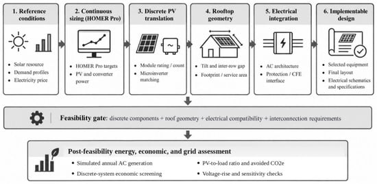
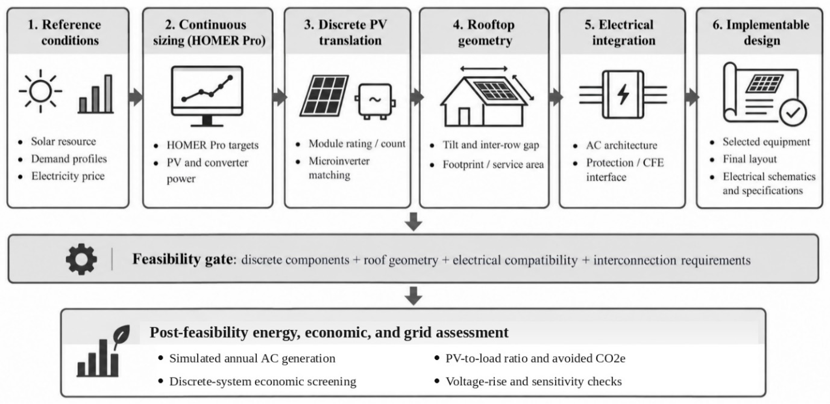
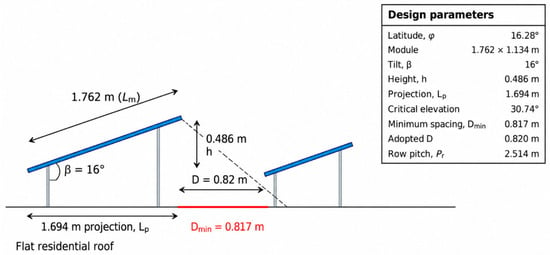
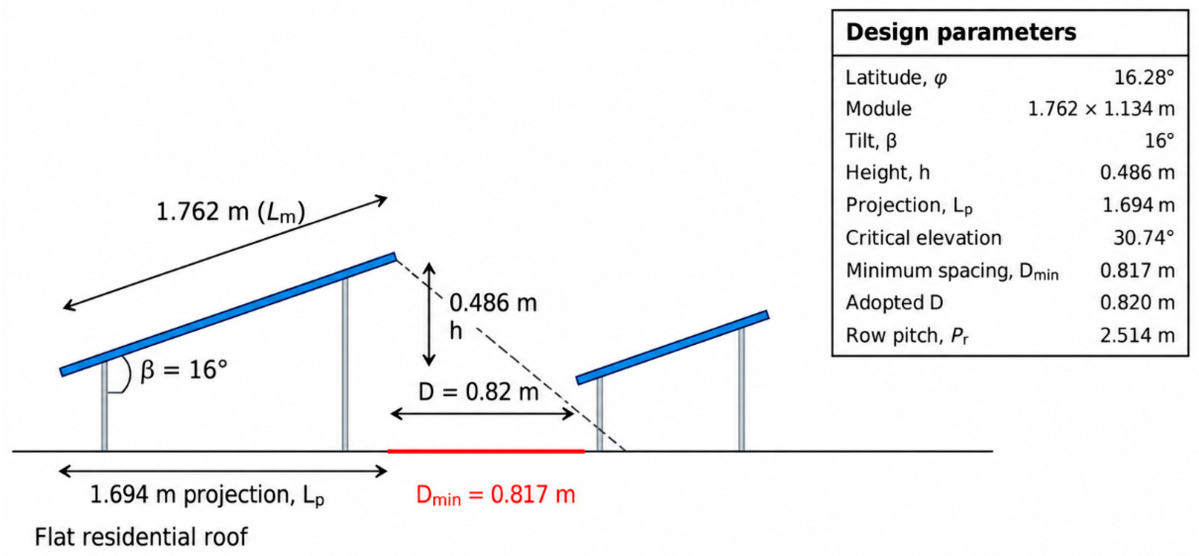
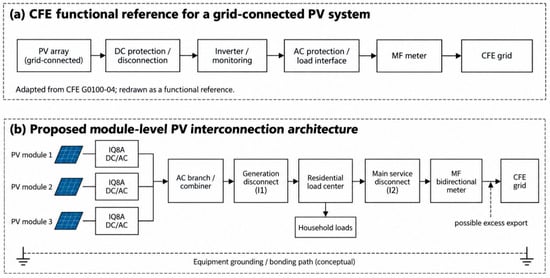
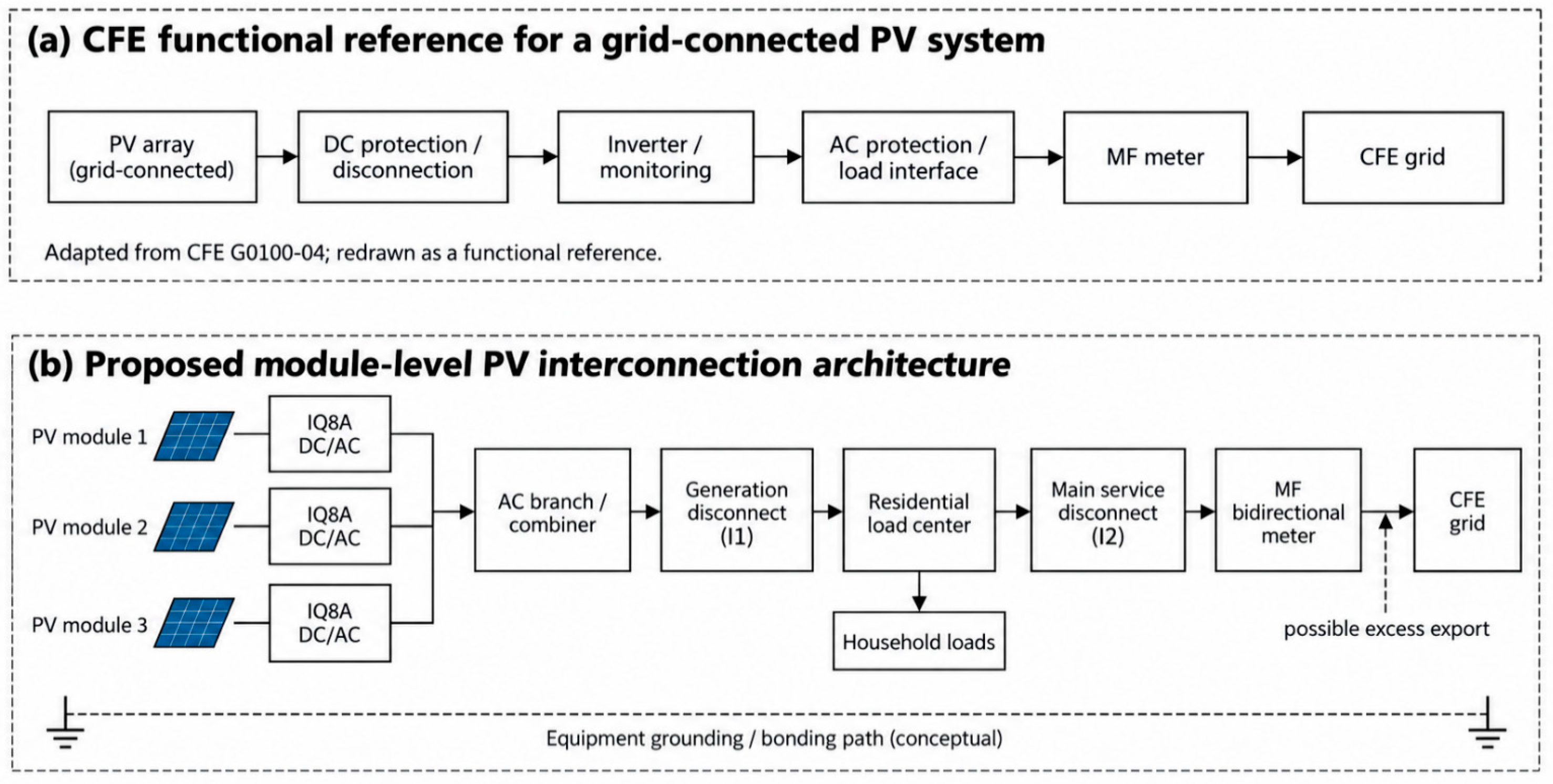
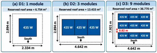
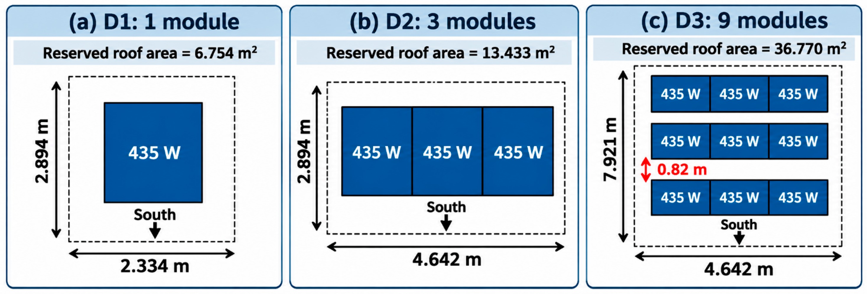
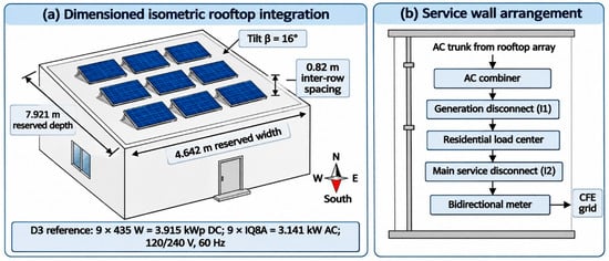
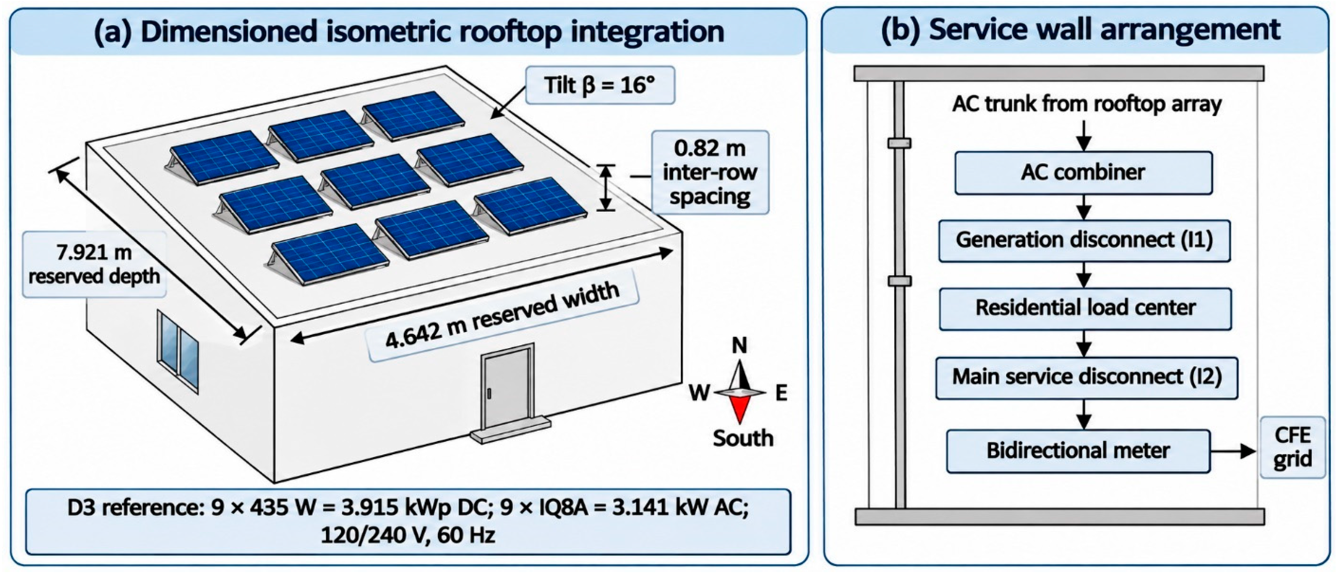

Disclaimer/Publisher’s Note: The statements, opinions and data contained in all publications are solely those of the individual author(s) and contributor(s) and not of MDPI and/or the editor(s). MDPI and/or the editor(s) disclaim responsibility for any injury to people or property resulting from any ideas, methods, instructions or products referred to in the content. |
© 2026 by the authors. Licensee MDPI, Basel, Switzerland. This article is an open access article distributed under the terms and conditions of the Creative Commons Attribution (CC BY) license.