


Abstract
Magnetic treatment of injection water has been proposed as a low-cost, chemical-free means of improving waterflooding, but laboratory evidence that links field intensity, pressure, electrokinetic behaviour and oil displacement remains limited. This study investigates the effect of a constant transverse magnetic field (40–150 mT) applied to injection water upstream of a linear sand–clay (75:25) porous-medium model, 120.4 cm long and 4.2 cm in internal diameter. First, single-phase water flow was examined at 1.6–30.4 atm, recording the potential difference, electrical resistance and outflow rate. Second, three oils with kinematic viscosities of 24.9 mm2/s (paraffin oil), 47.49 mm2/s (machine oil) and 198 mm2/s (refined transformer oil) were displaced by untreated and magnetically treated water at pressures up to 35.2 atm. Magnetic treatment lowered the potential difference and resistance of the water-saturated medium and increased the water outflow rate. In oil displacement, the final oil displacement coefficient increased from 47.38% to 60.64% for machine oil, from 42.30% to 54.32% for paraffin oil and from 37.08% to 50.36% for transformer oil at the most effective intensity of 125 mT, while the water displacement coefficient decreased. Magnetic treatment also stabilised the electrokinetic response during displacement. A generalised filtration law that includes electromagnetic forces is presented; with the streaming field taken from the measured potential difference, it reproduces the single-phase data up to 20.8 atm at all intensities with one parameter set (R2 = 0.967) and shows that treatment mainly lowered the threshold pressure difference, from 4.1 to 0.9 atm at 125 mT. Untreated control runs in the same setup, the non-monotonic dependence on field intensity and heat-balance estimates indicate that heating, vibration and degassing do not explain the effects. The between-run uncertainty of the oil displacement coefficient is estimated at 1–2 percentage points.
1. Introduction
Improving the development efficiency of oil fields is of major importance for the effective use of energy resources. Conventional production methods recover only part of the oil in place, and the volume of residual oil remaining in reservoirs is commonly reported to be 50–60% [1,2]. Enhanced oil recovery (EOR) methods are traditionally divided into primary, secondary and tertiary stages that follow the chronological sequence of reservoir production [1,2]. Primary recovery relies on the natural energy of the reservoir, secondary recovery is today largely synonymous with waterflooding, and tertiary methods—thermal, physicochemical and physical–hydrodynamic—are applied when waterflooding becomes uneconomic [1,2,3].
EOR processes can be classified into mobility-control, chemical, miscible, thermal and other (for example, microbial) processes [4,5,6,7]. Polymer flooding improves macroscopic sweep by reducing the mobility of the displacing water [4]; surfactant-based processes reduce interfacial tension between the displacing fluid and oil [5,6]; and thermal processes reduce oil viscosity and are preferred for heavy, low-API oils [7,8]. Each of these approaches has limitations related to cost, reservoir conditions or environmental impact, which motivates continued research on alternative technologies [9].
Although waterflooding is the most widely applied recovery technique, it is affected by low displacement efficiency, high water cut and problems caused by reservoir heterogeneity [10,11,12]. These limitations have directed researchers towards methods based on physical fields—magnetic, electric or ultrasonic. Among them, electromagnetic heating of heavy oil has received considerable attention [13], whereas the magnetic treatment of injection water, which does not rely on heating, has been studied much less.
Exposure of water to a magnetic field can change its structural and dynamic properties, including viscosity, ion mobility and surface tension, and can reduce scale formation [14]. These changes may alter the interaction between the injected fluid and the reservoir rock and thereby improve the displacement of trapped oil. The effectiveness of magnetic treatment depends on the correct choice of field intensity: several earlier attempts to increase oil recovery by magnetically treated water gave unsatisfactory or even negative results, which has been attributed to the use of an alternating field or to an incorrectly chosen field intensity [14]. Laboratory and field studies carried out at the Department of Oil and Gas Engineering of the Azerbaijan State Oil and Industry University since the 1970s showed that treating injection water with a constant transverse magnetic field increased the injectivity of injection wells by about 30% and increased the production of surrounding wells, while reducing corrosion of field equipment [14]. Independent studies of magnetic water treatment have, however, produced both positive and negative results, and the reproducibility of the effects is still debated; the present results are compared with the literature in Section 5.5.
The interaction of a magnetic field with reservoir fluids is explained by electrokinetic theory. When a liquid moves through a porous medium, a streaming potential (the Quincke effect) is generated and the pore surface becomes electrically charged; this excess potential is considered to oppose fluid motion and to reduce the permeability of the rock [14,15]. Darcy’s law, and its generalisation by A.Kh. Mirzajanzade, who introduced the initial pressure gradient for the flow of non-Newtonian oils [15,16], take into account the properties of the saturating fluids and rocks but not the electromagnetic interactions that arise during flow.
Earlier work on the same experimental system examined the effect of magnetic field treatment on fluid flow in porous media [17], characterised the untreated injection water [18] and the gas permeability of the sand–clay model [19]; the magnetic treatment device is described in [20]. Permeability determination and water–oil displacement were performed according to established laboratory procedures [2,21]. The present article brings together, in one consistent framework, (i) a generalised filtration law that includes electromagnetic forces, (ii) laboratory measurements of the potential difference, electrical resistance and outflow rate of water flowing through a sand–clay porous medium under magnetic fields of 40–150 mT and pressures of 1.6–30.4 atm, and (iii) water-displacement experiments with three oils of different physicochemical properties using untreated and magnetically treated water. The objective is to determine how the magnetic field intensity and pressure affect the flow and electrokinetic behaviour of water and the oil displacement efficiency, to identify the most effective field intensity for oils of different viscosity, to test the generalised filtration law quantitatively against the measurements, and to assess possible experimental artefacts, the measurement uncertainty and the requirements for field application.
2. Theoretical Background: Generalised Filtration Law Including Electromagnetic Forces
Darcy’s law, in the form used in oil production, is written as [21]
where Q is the flow rate of the liquid through the porous medium, k0 is the initial permeability of the porous medium, P1 and P2 are the pressures at the inlet and outlet of the sample, S is the filtration area, μ is the viscosity of the filtered liquid and l is the length of the porous medium.
Before development, the surface of the porous reservoir medium possesses an initial magnetic field strength determined by the adsorption layer on the rock surface, which depends on the rock composition, the properties of the saturating fluid (mainly viscosity), the depth and the coordinates of the reservoir. At the start of flow, the rock has an initial permeability k0 and an initial production rate Q0. Once the fluid moves, a streaming potential is generated, and the pore surface is charged to a potential that depends on the electrical capacitance of the rock, in the manner of a capacitor. The excess potential is radiated by the pore surface as an electromagnetic field that hinders fluid motion and reduces permeability. Laboratory filtration of gas-free Devonian oil through sandstone showed a high initial production rate followed by a significant decline [14,15]. These observations make it necessary to account for electromagnetic forces in Darcy’s law.
A charge q moving with velocity υ experiences, in addition to the electric force qE, a magnetic force, so that the total electromagnetic force is
F = qE + qυ × B
For a charge moving along the Ox axis with the field directed perpendicular to that axis, and with B denoted by H as in the original derivation (H is the magnetic induction of the applied field measured by the magnetometer, expressed in T; the values in mT reported below are induction values, so that the product qυH has the dimension of force, C·m·s−1·T = N), the projection of the electromagnetic force is
FEM = qE + qυH
To introduce the electromagnetic forces into Equation (1), the flow rate and pressures are expressed through the filtration velocity υ and the forces F1 and F2 acting on the inlet and outlet faces:
Substituting Equation (4) into Equation (1) and rearranging gives
Adding the streaming-potential (Quincke) contribution and the electromagnetic force (3) to the right-hand side yields
Collecting the terms in υ, dividing by S, using P = F/S and multiplying by S, the generalised law of liquid filtration in a porous medium is obtained:
For E = 0 and H = 0, Equation (7) reduces to Darcy’s law (1). The values of E, q and H entering Equation (7) are to be determined experimentally during filtration. Equation (7) shows that, within this framework, the filtration rate and therefore the amount of oil recovered can be changed by adjusting the strength of the applied magnetic field.
Dimensions and signs: In Equation (7), all terms of the numerator are forces (N), and both terms of the denominator have the dimension of a flow resistance per unit area, N·s·m−3: μl/k0 [Pa·s·m·m−2 = N·s·m−3] and qH/S [C·T·m−2 = N·s·m−3]; Q is therefore obtained in m3/s. E is the axial electric field generated in the porous medium by the flow itself (the streaming field) and is obtained from the measured potential difference U between the electrodes as E = U/l. Because the streaming field is directed against the flow, the electric term retards filtration, i.e., qE is negative in the flow direction. Equation (7) can then be written as Q = (S/D)(ΔP − ΔP0), where D = μl/k0 − qH/S is the effective flow resistance and ΔP0 = q|E|/S is a threshold pressure difference—the electrokinetic analogue of the initial pressure gradient introduced by Mirzajanzade for clay-bearing media [15,16]. The magnetic term carries a minus sign in the denominator because magnetic treatment increased the flow rate in the experiments, i.e., a positive qH/S lowers the effective resistance; the denominator must remain positive (qH/S < μl/k0), which bounds the admissible magnitude of this term.
Physical meaning of q: In Equation (7), q is not the charge of an individual ion or particle. It is the net mobile (excess) charge of the diffuse part of the electrical double layer contained in the pore space of the sample, i.e., the counter-ion charge that compensates the negative surface charge of the clay and quartz and is carried by the flow, producing the streaming current and potential [14,15]; its magnitude is bounded by the exchange capacity of the solid (Section 4.4). It should also be stressed that the Lorentz force qv × B acting on a charge that moves along the flow axis is perpendicular to that axis, so that a transverse field cannot accelerate the flow directly. Moreover, in the present setup the water is treated upstream of the column, and the porous medium itself is outside the field. The term qH/S is therefore interpreted as an effective (phenomenological) term that represents the reduction in the electrokinetic flow resistance of water that has passed through the field—through the field-induced redistribution of ions and change in hydration structure, which relaxes over a finite time [14]—with H the induction of the treatment field. Within this interpretation, q, E and H are quantities determined from the filtration experiment, and Equation (7) is tested against the measured data in Section 4.4. All three are effective, sample-averaged quantities rather than local fields: E is the mean axial streaming field over the sample length, q the total mobile excess charge in the sample, and H the induction in the treatment zone upstream of the column, not a local field inside the medium. If the magnetic field strength in A/m were used instead of the induction, the force term in Equations (3) and (6) would be qυμ0H (μ0 = 4π × 10−7 H/m) and H would have to be replaced by μ0H in Equation (7); because H denotes the induction in T throughout this paper, no such factor is needed. The term “generalised filtration law” is used in the sense of a phenomenological relation: Equation (7) is validated quantitatively here only for the ascending branch of the single-phase data (Section 4.4); outside that range it should be regarded as a qualitative framework.
3. Materials and Methods
3.1. Porous Medium
A linear reservoir model consisting of a high-pressure column with an internal diameter of 4.2 cm and a length of 120.4 cm was used. The inner wall of the column was coated with epoxy adhesive, which was distributed uniformly by periodically rotating the tube and allowed to cure fully at room temperature for several days. The coating electrically insulated the porous medium from the column body and prevented fluid bypass along the wall. The column was filled with a mixture of 75% quartz sand and 25% clay (mass ratio 3:1). To obtain a compact medium, each new portion of the mixture was added and compacted by vertical vibration and tamping, after which the upper flange was tightened to apply an overburden load; filling continued until vibration and load no longer changed the degree of compaction, so that a pressure-independent permeability was obtained. The mass of the empty column was 6.075 kg and that of the filled column 7.245 kg. Both ends of the column were closed with metal heads sealed with rubber rings and equipped with pressure gauges and high-pressure valves. The tightness of the system was checked at 1–2 atm before each experiment. The sand component consisted of quartz (SiO2), in which each silicon atom is tetrahedrally coordinated by four oxygen atoms (Si–O bond length about 1.60 Å). The clay component was illite, a layered aluminosilicate whose SiO2 tetrahedral and Al2O3 octahedral sheets are held together by interlayer potassium (K+) ions; on contact with water, the clay swells as water enters the interlayer space, and an electrical double layer and zeta potential form on the negatively charged clay surfaces, which affect the filtration and permeability of clay-bearing rocks. The air permeability of the porous medium was determined by a standard method, and the pore volume was determined both gravimetrically and by filling the medium with air to a given pressure and applying the gas equation of state. The bulk volume of the packed medium is 1668 cm3. Because saturation was performed after evacuation, the pore volume was estimated as the volume of oil retained in the medium at the end of each saturation (injected minus recovered volume; Section 3.5): 420, 435 and 445 mL in the untreated experiments with machine, paraffin and transformer oil, and 376–440 mL in the experiments with treated water, corresponding to an effective porosity of 0.23–0.27 (mean 0.25). The water permeability determined from the linear part of the untreated flow rate–pressure dependence (Section 4.4) by Darcy’s law (μ = 1.0 mPa·s, l = 1.204 m, S = 13.85 cm2) was 47 ± 6 mD, whereas the apparent permeability calculated point by point increased from 9 mD at 1.6 atm to 43 mD at 20.8 atm. The grain-size distribution of the sand and clay fractions was not measured. Compaction was controlled by packing to refusal under vibration and overburden load, as described above, and by weighing the column; the reproducibility of the pore space between experiments was assessed from the retained oil volumes, whose coefficient of variation between runs was 4.1%, 2.5% and 2.5% for the machine, paraffin and transformer oil series, respectively. For reference, the gas permeability of a sand–clay model of the same composition and dimensions, packed by the same procedure (packed mass 1665 g), was measured with nitrogen, methane and carbon dioxide at pressure differences of 1.25, 2.5 and 5 atm [19]. At a pressure difference of 1.25 atm, the initial permeability was 4.88 mD (N2), 3.78 mD (CH4) and 3.06 mD (CO2); it decreased sharply during the first 100 s of flow and with increasing pressure difference, reaching 0.25, 0.17 and 0.20 mD, respectively, at 5 atm.
To measure the potential difference across the porous medium, high-resistance nichrome wire electrodes were used. Each wire was in contact with the porous medium at one end and was surrounded by a fluoroplastic layer that insulated it from the rock while remaining conductive with respect to the liquid.
3.2. Fluids
Tap water was used as the displacing agent. Its physicochemical properties were analysed before and after magnetic treatment (Table 1). The differences between the two analyses are small, are discussed critically in Section 5.3 and are reported as indicative only. Both analyses were performed on the same tap water: the column “before magnetic treatment” corresponds to the analysis of the untreated tap water reported in [18], and the column “after magnetic treatment” to the analysis of water sampled after passage through the energised electromagnet. The values were verified against the original analysis records.
Table 1.
Physicochemical properties of the tap water before and after magnetic treatment.
Three oils with different physicochemical properties were used as model oils representing crude oils of different rheology: refined transformer oil, machine oil and paraffin oil. Their kinematic viscosities were measured with an Engler capillary viscometer and their densities with a hydrometer (Table 2).
Table 2.
Properties of the oils used in the experiments.
3.3. Experimental Setup
The experimental setup is shown in Figure 1 and Figure 2. It consists of a USA-4A regulator (1), a SUNTEK 2000 VA voltage regulator (2), a volt-ammeter (3), an electromagnet (4), a measuring cylinder (5), valves (6, 10, 13, 15, 17), pressure gauges (7, 9, 16), the high-pressure column (8), a URV-2M high-input-impedance potentiometer (11), a thermostat (12), a PVT-type high-pressure bomb (14), a liquid tank (18) and a measuring press (19).
Figure 1.
Schematic diagram of the experimental setup for displacement with magnetically treated water: 1—USA-4A regulator; 2—SUNTEK 2000 VA voltage regulator; 3—volt-ammeter; 4—electromagnet; 5—measuring cylinder; 6, 10, 13, 15, 17—valves; 7, 9, 16—pressure gauges; 8—high-pressure column; 11—URV-2M potentiometer; 12—thermostat; 14—PVT-type high-pressure bomb; 18—liquid tank; 19—measuring press.
Figure 2.
Photograph of the experimental setup.
The PVT bomb has a volume of 800 mL, a diameter of 8 cm and a height of 20 cm. It was filled with water and connected to the column through a copper tube passing through the field of the electromagnet. The tubing must be made of a non-magnetic material that does not screen the magnetic field; copper was used in this study. Machine oil, used as the pressure-transmitting agent, was supplied from the tank to the bomb by the measuring press; the oil entering the bomb from below moved the piston, which displaced the water from the bomb into the porous medium.
The electromagnet was installed on the line near the column inlet (Figure 3); its power is 1.3 kW, its operating current 4.2 A and its voltage 220 V. The electromagnet was intended to expose the water to the magnetic field before it entered the column. Because the electromagnet operates with a constant magnetic field but is fed from an alternating-current source, a voltage regulator with a built-in rectifier was used to convert and regulate the current. Different magnetic induction values were obtained by changing the voltage U of the regulator, and the resulting field intensity H was measured with a magnetometer (Table 3). The device for magnetic treatment of injection water is protected as a utility model [20]. In the DC regime, the maximum working current of the coil is 2 A; at the regulator voltages used (5–30 V; Table 3), the electrical power supplied to the coil therefore did not exceed 10–60 W, i.e., less than 5% of the rated power. The magnetic circuit has a length of 0.49 m, a core cross-section of 1000 mm2 and an air gap of 10 mm through which the copper tube passes; only the water in this tube section is exposed to the field, and the porous medium itself is outside the field. The pole faces have the cross-section of the core (1000 mm2), so that, for a square core section, the field acts over a length of about 32 mm along the tube. Because the copper tube passes through the 10 mm air gap, its outer diameter cannot exceed 10 mm; for an internal diameter of 8 mm or less, the volume of water in the field is at most 1.6 cm3. The induction was measured with the magnetometer at the centre of the gap; its uniformity across the tube and the fringe-field gradient at the pole edges were not mapped. The residence time of the water in the field depends on the flow rate: in the water-flow experiments, where the outflow rate ranged from 0.1 to 9.2 cm3/min, it was at most about 16 min at the lowest and about 10 s at the highest rates, whereas in the displacement experiments the mean throughput (468–600 mL in 110 min, i.e., 4.3–5.5 cm3/min) differed by less than 13% between runs, so that the residence time (at most about 20 s) was nearly the same in all displacement runs. Neither the setup nor the column was magnetically shielded; the Earth’s field (about 50 µT) is less than 0.13% of the lowest applied induction, and the stray field of the electromagnet at the column was not measured.
Figure 3.
Schematic of the magnetic treatment device: 1—copper tube carrying the liquid; 2—electromagnet core; 3—copper windings; 4—step-down transformer; 5—voltage regulator.
Table 3.
Calibration of the magnetic field intensity against the regulator voltage.
3.4. Procedure for Water Flow Experiments
The porous medium and the test liquid were evacuated beforehand, and the medium was then saturated from the PVT bomb; about ten pore volumes of liquid were passed through it. To remove air completely, the pressure in the system was periodically raised and the liquid was then sharply released.
Before each experiment, the initial potential difference and resistance were recorded. Oil was then pumped into the bomb by the measuring press at 1.6 atm, displacing the water from the bomb into the porous medium, and the pressure was held constant. After a 2 min waiting period to allow complete saturation of the medium with water, the column outlet was opened, the volume of outflowing water was measured with the measuring cylinder, and the resistance and potential difference were recorded simultaneously. The procedure was repeated at pressure steps of 3.2 atm up to 30.4 atm, without a magnetic field and at field intensities of 40, 80, 107, 125, 140 and 150 mT. These intensities were selected on the basis of the literature, preliminary experimental results and practical feasibility under field conditions. All experiments were performed with the column connected to the thermostat (12) at 20 °C, the temperature at which the fluid properties in Table 2 were determined. No gas was dissolved intentionally: the liquids and the medium were evacuated before saturation, the system contained no free gas phase, and the pressure in the column was never lower than 1.6 atm. Each pressure step was held for 2 min before the outflow, resistance and potential difference were recorded, so that the water-flow data correspond to quasi-stationary conditions at each step; the pressure was increased in steps of 3.2 atm. The untreated (0 mT) runs were performed in the same setup, with the water passing through the copper tube inside the de-energised electromagnet, and serve as controls for the runs with the field switched on.
3.5. Procedure for Oil Displacement Experiments
The porous medium was saturated with the oil under study using the PVT bomb after the oil and the medium had been evacuated with a vacuum pump; the pressure was periodically raised and the oil sharply released to remove residual air. The oil was transferred in a single-phase state from the bomb into the medium by means of the press. For each oil, 800 mL was injected, and the oil volume collected at the outlet at the end of injection was recorded: 355 mL (44.4%) for transformer oil, 380 mL (47.5%) for machine oil and 365 mL (45.6%) for paraffin oil. No ageing period was applied after saturation: the refined model oils contain no crude-oil polar components that could alter the wettability of the medium during ageing, so the experiments represent displacement from a medium that was initially water-free and not deliberately oil-aged. The retained volume (800 mL minus the volume collected at the outlet) includes the oil held in the inlet and outlet lines and valves, which was not measured separately. Because the same lines were used in all runs, this holdup biases the absolute values of ηoil (the retained volume overestimates the oil in the pore space) but not the comparison between runs.
The oil remaining in the medium was then displaced by water. The bomb piston was lowered by applying 4–5 atm of gas (nitrogen or carbon dioxide), the bomb was evacuated for 10–15 min, and 800 mL of water was admitted through a funnel while preventing air entry. The water was then displaced from the bomb into the porous medium by the press. The pressure was increased stepwise by 1.6 atm every 5 min, from 1.6 atm to 35.2 atm. At each 5 min interval, the volume of water entering the system, the potential difference, the resistance and the volumes of oil and water leaving the column were recorded. The oil displacement coefficient ηoil and the water displacement coefficient ηw are reported as percentages, with ηoil relative to the oil volume retained in the medium after saturation and ηw relative to the 800 mL of water in the bomb. Volumes were read to the nearest 0.5–1 mL. Because the pressure was increased stepwise by 1.6 atm (on average 0.32 atm/min), the displacement experiments are unsteady-state floods; each 5 min stage is quasi-stationary only with respect to the applied pressure. The phase volumes were read in the measuring cylinder; emulsion formation was not characterised. With regard to steady state, the characteristic time for pressure equilibration over the column, L2φμct/k, is about 8 s for water (taking ct ≈ 1 × 10⁻⁹ Pa−1 and k = 47 mD), so the single-phase water-flow data recorded after a 2 min hold are quasi-stationary. For the oils (dynamic viscosities of 20.9, 40.4 and 192 mPa·s for paraffin, machine and transformer oil) the corresponding times are about 3, 5 and 25 min, comparable to or longer than the 5 min step; together with the evolving saturation, this means that the displacement experiments are transient and that their results are specific to the pressure schedule, which was identical in all runs.
The displacement experiments with magnetically treated water followed the same procedure, with the electromagnet operating at 40, 80, 107, 125, 140 or 150 mT. In these experiments, results were recorded every 10 min (every 3.2 atm). Before each experiment with treated water, the medium was saturated with oil by the same procedure; the retained oil volumes were 410, 392, 380, 376, 385 and 390 mL (machine oil), 425, 420, 410, 405, 410 and 420 mL (paraffin oil) and 440, 430, 425, 415, 420 and 425 mL (transformer oil) at 40, 80, 107, 125, 140 and 150 mT, respectively, and ηoil of each run was calculated relative to its own retained volume. As in the water-flow experiments, the untreated displacement runs were performed with the water passing through the de-energised electromagnet.
3.6. Flow of the Oils Under Normal Conditions
To determine the flow behaviour of the oils outside the porous medium, a separate setup consisting of a liquid tank, pressure gauge, valve, measuring press and measuring cylinder was used. The flow rate of each oil, and of water for comparison, was measured as a function of time and pressure; the experiments were repeated several times. The setup consists of (1) a liquid tank, (2) a pressure gauge, (3) a valve, (4) a measuring press and (5) a measuring cylinder, connected in series by high-pressure tubing. The test liquid is displaced from the tank by the measuring press, the pressure is read on the gauge, and, when the valve is opened, the liquid flows through the valve into the measuring cylinder, where the collected volume is read at 2 min intervals while the pressure is raised in steps of 0.5 atm from 0.5 to 2.0 atm (Table 4). The flow path contains no porous medium, so the measurements characterise the bulk flow behaviour of the liquids; water, a Newtonian liquid, was used as a reference to check the setup. Because the arrangement is a simple series connection of standard components, it is described in the text rather than in an additional figure.
Table 4.
Flow rates of water and oils under normal conditions (outside the porous medium).
3.7. Control of Geomagnetic Activity
Geomagnetic storms are disturbances of the Earth’s magnetic field [22] that can affect electromagnets, systems based on electromagnetic fields and sensitive experimental equipment, causing measurement errors. The geomagnetic activity level in Baku during October 2024, when the experiments were conducted, was evaluated on an eight-level scale (1—no significant disturbance; 2—minor disturbances; 3—weak storm; 4—small storm; 5—moderate storm; 6—strong storm; 7—severe storm; 8—extreme storm) [23]. Experiments were carried out on days with “minor disturbances”, and the geomagnetic activity was monitored in real time on each day of the magnetic experiments. In practice, this was done as follows. The three-hourly activity index for Baku [23] was checked before each experiment and during it. In October 2024 the index remained at levels 1–2 throughout the day on 1, 2, 9, 14, 22, 23, 30 and 31 October and during working hours on several other days, whereas strong to extreme storms (levels 6–8) occurred on 4–5 and 10–11 October. Experiments with the electromagnet were performed only in intervals in which the index did not exceed level 2; an experiment would have been discarded and repeated if the index had risen to level 3 or higher during the run, but no such rise occurred during the reported experiments, so no data were excluded or corrected. It should also be noted that even severe geomagnetic storms change the Earth’s field by no more than the order of 102–103 nT, i.e., by less than 3 × 10⁻⁵ of the lowest applied induction (40 mT); their influence on the treatment field itself is therefore negligible, and the precaution concerns mainly the sensitive millivolt-level electrical measurements.
4. Results
4.1. Water Flow Through the Porous Medium Under Magnetic Treatment
The potential difference, resistance and water outflow rate measured as functions of pressure are shown in Figure 4.
Figure 4.
Effect of pressure and magnetic field intensity on water flow through the porous medium: (a) potential difference; (b) electrical resistance; (c) water outflow rate. Each curve is a single run (n = 1), so the error bars are not standard deviations of replicate experiments; they show the 95% expanded uncertainty (k = 2) of a single reading (Section 5.7): ±1.8 mV for the potential difference, ±4% of the value for the resistance and ±0.12 cm3/min for the outflow rate.
Without a magnetic field, the potential difference decreased from 92.2 mV at 1.6 atm to 45.4 mV at 20.8 atm and then increased slightly to 48.5 mV at 30.4 atm (Figure 4a). The resistance followed the same pattern, decreasing from 140.8 kΩ to a minimum of 74.6 kΩ at 20.8 atm and then increasing to 90.4 kΩ at 30.4 atm (Figure 4b). The water outflow rate increased from 0.1 cm3/min at 1.6 atm to a maximum of 6.2 cm3/min at 20.8 atm and decreased to 3.8 cm3/min at 30.4 atm (Figure 4c).
With magnetic treatment, the potential difference and resistance decreased more steeply as pressure increased and stabilised at lower values than in the untreated case. For all field intensities, the minima of the potential difference and resistance occurred at 20.8 atm. The lowest values were obtained at 125 mT: 20.2 mV and 40.3 kΩ at 20.8 atm, compared with 45.4 mV and 74.6 kΩ without the field. Above 20.8 atm, the resistance under magnetic treatment remained below the untreated values at all pressures; at 30.4 atm, it was 59.1 kΩ at 125 mT and 62.2 kΩ at 107 mT, compared with 90.4 kΩ without the field. At the lowest pressure (1.6 atm), the effect of the field on the potential difference was not uniform: values both above (97.7 mV at 107 mT) and below (74.6 mV at 125 mT) the untreated value were recorded.
Magnetic treatment increased the water outflow rate at all pressures. Up to 20.8 atm, the outflow rate increased with field intensity, reaching a maximum of 9.2 cm3/min at 150 mT and 20.8 atm. Above 20.8 atm, the outflow rate decreased for all conditions, but remained above the untreated values; at 27.2 atm and 30.4 atm, the highest outflow rates were obtained at 107 mT (6.8 and 6.0 cm3/min, respectively). Relative to untreated water, the outflow rate at 20.8 atm increased by 10%, 16%, 29%, 35%, 42% and 48% at 40, 80, 107, 125, 140 and 150 mT, respectively, and at 4.8–8.0 atm it increased by factors of 2–7. The decrease in outflow rate above 20.8 atm occurred under all conditions and coincided with an increase in resistance and potential difference (Figure 4a,b); it is attributed to a pressure- and time-dependent reduction in the permeability of the clay-bearing medium, as discussed in Section 5.1.
4.2. Water Displacement of Oils Without Magnetic Treatment
The results of displacing the three oils with untreated water are shown in Figure 5. Oil first appeared at the outlet after 10 min (3.2 atm) for machine oil and after 20 min (6.4 atm) for paraffin and transformer oils, and water first appeared after 35 min (11.2 atm) in all three experiments. At the end of displacement (110 min, 35.2 atm), 199 mL of oil and 340 mL of water were produced for machine oil (ηoil = 47.38%, ηw = 42.50%), 184 mL of oil and 400 mL of water for paraffin oil (ηoil = 42.30%, ηw = 50.00%), and 165 mL of oil and 435 mL of water for transformer oil (ηoil = 37.08%, ηw = 54.38%). Machine oil thus showed the highest oil displacement and the lowest water production, and transformer oil the lowest oil displacement and the highest water production (Figure 5a,b). The displacement coefficients in Figure 5 and Figure 6 were calculated directly from the recorded cumulative volumes, with ηoil relative to the retained oil volume (420, 435 and 445 mL for machine, paraffin and transformer oil) and ηw relative to 800 mL. All cumulative coefficients increase monotonically with time. For machine oil, ηoil rises most rapidly between 55 and 100 min (17.6–32.0 atm), when oil production accelerated, and levels off thereafter as the water fraction in the outflow increased. Under incompressible flow, the volume of water injected equals the total volume produced; at the end of the untreated experiments, 539, 584 and 600 mL of water had been injected (1.28, 1.34 and 1.35 retained pore volumes) for machine, paraffin and transformer oil, of which 199, 184 and 165 mL replaced the produced oil in the medium and 340, 400 and 435 mL left the column. The oil remaining in the medium was therefore 221, 251 and 280 mL, and the cumulative water–oil ratio 1.71, 2.17 and 2.64. Water first appeared at the outlet after a throughput of only 5–11 mL (about 0.01–0.03 pore volumes), which indicates that it broke through along preferential paths (viscous fingering at oil-to-water viscosity ratios of about 21–192) rather than as a piston-like front. A dead volume in the outlet line would delay rather than advance breakthrough; the breakthrough pressures are therefore controlled by fingering and by the low flow rates during the first pressure steps, and their resolution is limited by the recording interval (1.6 atm, or 3.2 atm in the treated runs).
Figure 5.
Displacement of the three oils by untreated water as a function of time (pressure increased by 1.6 atm every 5 min from 1.6 to 35.2 atm): (a) oil displacement coefficient; (b) water displacement coefficient; (c) electrical resistance; (d) potential difference.
Figure 6.
Oil displacement coefficient (a–c) and water displacement coefficient (d–f) as functions of pressure for displacement with untreated water and water treated at 40–150 mT: (a,d) machine oil; (b,e) paraffin oil; (c,f) transformer oil.
During the first 60 min, the resistance changed only slightly for all oils (Figure 5c), indicating a relatively weak interaction with the rock during this period. After about 1 h, the resistance changed noticeably. For paraffin oil, the resistance decreased from 190 kΩ at the start to 120 kΩ at 85 min and 110 kΩ at the end; for transformer oil, it decreased gradually from 170 kΩ to about 100 kΩ; and for machine oil, it decreased from 140 kΩ to 80–100 kΩ, with smaller variations. The potential difference was highest for paraffin oil (78.6 mV initially and 60.4 mV at the end), intermediate for transformer oil (70.6 to 52.9 mV) and lowest for machine oil (57.8 to 42.4 mV) (Figure 5d).
The flow rate of each oil as a function of pressure during displacement indicated viscoplastic behaviour of all three oils inside the porous medium: the oil flow rate remained very low up to about 14 atm and increased sharply above 16 atm. In contrast, under normal conditions outside the porous medium, the flow rates of the oils increased with pressure in the manner of viscous liquids, and water behaved as a Newtonian liquid (Table 4).
4.3. Water Displacement of Oils with Magnetically Treated Water
The oil and water displacement coefficients obtained with untreated and magnetically treated water are shown in Figure 6 as functions of pressure, and the final values are summarised in Table 5 and Figure 7.
Table 5.
Final oil and water displacement coefficients (%) at 35.2 atm for displacement with untreated and magnetically treated water. Single runs (n = 1). The standard uncertainty of ηoil is relative and therefore proportional to the value: 4.1%, 2.5% and 2.5% of ηoil for machine, paraffin and transformer oil (±1.9–2.5, ±1.1–1.4 and ±0.9–1.3 percentage points); the standard uncertainty of ηw is ±0.72 percentage points (Section 5.7).
Figure 7.
Final displacement coefficients at 35.2 atm as functions of magnetic field intensity (0 = untreated water; categories are evenly spaced): (a) oil displacement coefficient; (b) water displacement coefficient. Each point is a single run (n = 1), so the error bars are not standard deviations of replicate experiments; they show the 95% expanded uncertainty estimated for an individual run (Section 5.7): for ηoil, ±2 × the relative reproducibility of the retained oil volume (4.1%, 2.5% and 2.5% of the value for machine, paraffin and transformer oil), so the bar length is proportional to ηoil; for ηw, ±1.6 percentage points (t = 2.18 for 12 degrees of freedom × the pooled ANOVA residual of 0.72 percentage points).
For all three oils, the oil displacement coefficient increased with pressure, and magnetic treatment gave higher final oil displacement than untreated water (Figure 6a–c). For paraffin and transformer oils, the oil displacement coefficient with treated water exceeded the untreated values from 6.4 atm onwards. For machine oil, the treated-water values were mostly below or close to the untreated values up to 25.6 atm and exceeded them at all intensities from 28.8 atm onwards. The highest final oil displacement coefficient was obtained at 125 mT for all three oils: 60.64% for machine oil, 54.32% for paraffin oil and 50.36% for transformer oil, compared with 47.38%, 42.30% and 37.08%, respectively, without the field. At 140 and 150 mT, the final oil displacement coefficient was lower than at 125 mT but remained higher than without the field (Table 5).
Magnetic treatment reduced water production (Figure 6d–f). For machine oil, water was first recorded on the 3.2 atm grid at 12.8 atm without the field (breakthrough occurred at 11.2 atm in the 1.6 atm record of Section 4.2), but only at 22.4 atm with treated water at all intensities. For paraffin and transformer oils, water first appeared at 12.8 atm in all cases, but the water displacement coefficient at high pressures was lower with treated water. The final water displacement coefficient was lowest at 125 mT for all three oils: 30.00% for machine oil, 40.00% for paraffin oil and 44.75% for transformer oil, compared with 42.50%, 50.00% and 54.38% without the field. At higher intensities, water production increased again (Table 5, Figure 7b). The conclusion does not depend on normalising ηw to the 800 mL of water in the bomb: expressed as the fraction of water in the total produced fluid, water production at 125 mT was 51%, 59% and 63% for machine, paraffin and transformer oil, compared with 63%, 69% and 73% for untreated water.
Magnetic treatment also changed the electrokinetic response of the medium during displacement. Without the field, the resistance and potential difference fluctuated and decreased during the experiments (values at the first and last points of the 3.2 atm grid, i.e., at 3.2 and 35.2 atm): from 120 to 90 kΩ and from 52.2 to 42.4 mV for machine oil, from 180 to 110 kΩ and from 73.2 to 60.4 mV for paraffin oil, and from 160 to 100 kΩ and from 67.8 to 52.9 mV for transformer oil. With magnetically treated water, these parameters remained nearly constant at all intensities: 90–100 kΩ and 42.1–44.1 mV for machine oil, 110–120 kΩ and 50.1–53.7 mV for paraffin oil, and 120–130 kΩ and 57.3–61.1 mV for transformer oil.
4.4. Comparison of the Generalised Filtration Law with the Experimental Data
Equation (7) was tested against the single-phase water-flow data of Section 4.1 (μ = 1.0 mPa·s, l = 1.204 m, S = 13.85 cm2). The streaming field was taken from the measured potential difference as E = U/l at each pressure and field intensity, and the magnetic term was written as qH/S = cHH, with H the treatment induction. For the ascending branch (1.6–20.8 atm; 49 data points at seven field levels), a single set of three parameters—k0 = 36.6 mD, q = 2.2 × 10³ C and cH = 1.06 × 10¹¹ N·s·m−3·T−1—reproduces the measurements with R2 = 0.967 and a root-mean-square error of 0.50 cm3/min. Without the magnetic term (cH = 0), the best fit is markedly worse (R2 = 0.848, root-mean-square error 1.08 cm3/min); the data therefore require both the electric term, through the measured reduction in U, and an additional field-dependent reduction in the flow resistance. Fitting the linear form Q = a(ΔP − ΔP0) separately at each intensity gave R2 = 0.917, 0.978, 0.977, 0.991, 0.984, 0.986 and 0.973 for 0, 40, 80, 107, 125, 140 and 150 mT. The slope a increased from 0.320 ± 0.043 to 0.471 ± 0.035 cm3·min−1·atm−1 (± one standard error), corresponding to an effective permeability of 46.5 mD (untreated), 51.5, 54.1, 57.8, 60.9, 64.0 and 68.4 mD, and the threshold pressure difference decreased from 4.06 ± 1.29 atm without treatment to 2.67, 2.08, 1.27, 0.85 ± 0.70, 0.15 and approximately 0 atm; the corresponding threshold gradient ΔP0/L decreased from 0.34 MPa/m to 0.07 MPa/m at 125 mT.
The fitted parameters are physically plausible, with one instructive exception. The effective electrokinetic charge q = 2.2 × 10³ C (7.8 × 10³ C when the untreated data are fitted alone) is of the same order as the total exchangeable charge of the clay fraction: approximately 290 g of illite (25% of the packed mass) with a cation exchange capacity of 10–40 meq/100 g [24] carries 2.8 × 10³–1.1 × 10⁴ C. In contrast, if the magnetic coefficient were interpreted literally as qH/S with a free charge q, it would require q = cHS ≈ 1.5 × 10⁸ C, four orders of magnitude more than any charge available in the system. This supports the interpretation given in Section 2: the magnetic term does not describe a direct Lorentz force on the pore fluid, which is outside the field and on which a transverse field exerts no axial force, but an effective reduction in the electrokinetic flow resistance of water that has passed through the field. The denominator of Equation (7) remains positive over the tested range (μl/k0 = 3.3 × 10¹⁰ N·s·m−3 versus cHH ≤ 1.6 × 10¹⁰ N·s·m−3 at 150 mT).
Two features of the measurements are not reproduced by Equation (7) with constant parameters. First, above 20.8 atm the equation predicts a further increase in the outflow rate (to 5.9–14.4 cm3/min at 24.0–30.4 atm), whereas the measured rate decreased (to 3.8–7.6 cm3/min); this branch requires a pressure-dependent permeability k0(ΔP) (Section 5.1). Second, with a constant magnetic coefficient, Equation (7) cannot predict an optimum intensity: the non-monotonic behaviour of the potential difference and resistance (minimum at 125 mT) and of the displacement coefficients enters only through the experimentally determined dependence of E (and q) on the treatment field. Equation (7) is therefore a consistent framework for interpreting the single-phase data below 20.8 atm, but it is not yet predictive outside the range in which its parameters were determined.
5. Discussion
5.1. Effect of Pressure and Magnetic Field on Water Flow
The non-linear dependence of the potential difference and resistance on pressure in the untreated case (Figure 4a,b) can be attributed to the complex response of electrokinetic processes in the porous medium to pressure. Initially, increasing pressure facilitated the penetration of water into the porous structure, ion transport became more ordered and the electrokinetic potential decreased, so that the flow of water and ions stabilised as the resistance decreased. With further increases in pressure, electrostatic interactions with the pore walls became stronger, which may explain the renewed increase in potential; the non-uniform distribution of ion concentration in the pore structure may also contribute. The decrease in outflow rate above 20.8 atm (Figure 4c) is consistent with a progressive reduction in the transmissibility of the medium at higher pressures, for example, by compaction of the clay-bearing medium or reorganisation of the conductive pathways after contact with water. A pressure-dependent permeability is also required to describe this branch with Equation (7) (Section 4.4) and is consistent with the decrease in gas permeability with increasing pressure difference measured on a medium of the same composition [19].
Three mechanisms can contribute to this reduction in permeability above 20.8 atm, and all are consistent with the simultaneous increase in resistance, which indicates a narrowing of the conductive pore cross-section. (i) Seepage-force compaction: because the outlet is at atmospheric pressure, the drag exerted by the flowing water on the grains increases with the applied pressure (the mean gradient reaches 2.6 MPa/m at 30.4 atm), and the effective stress in the medium, which is confined between fixed end flanges, increases towards the outlet by up to the applied pressure difference; the clay-bearing medium is therefore consolidated near the outlet, and its pore throats narrow. (ii) Migration of fines: at the higher interstitial velocities, clay particles can be detached from grain surfaces and retained in downstream pore throats. (iii) Clay hydration: the pressure steps were applied successively so that the illite was exposed to water for progressively longer times; continued hydration and swelling of the clay reduce the pore space in a time-dependent manner superimposed on the pressure effect. The gas-permeability measurements on a medium of the same composition similarly showed a sharp decrease in permeability with time and with increasing pressure difference [19]. Magnetically treated water reduced but did not eliminate the decline—the resistance stayed below the untreated values and the outflow rates above them at all pressures—which is consistent with a smaller degree of pore narrowing and with the reduced formation damage reported for magnetised water (Section 5.5).
Field intensity versus magnetic dose. Because the residence time of the water in the field is inversely proportional to the flow rate, the magnetic dose (induction × residence time) was not constant in the water-flow experiments: it was largest at low pressures, where the flow was slowest, and up to about 100 times smaller at 20.8 atm. Consistent with a dose dependence, the relative increase in outflow rate caused by treatment was largest at low pressures (factors of 2–7 at 4.8–8.0 atm) and smallest near 20.8 atm (10–48%). In these experiments, however, dose and pressure vary together and cannot be separated. In the displacement experiments, the throughput and hence the residence time were nearly the same in all runs (Section 3.3), so the comparisons between field intensities in Table 5 and Figure 7 correspond to an approximately constant residence time, and the dose there is approximately proportional to the induction. Experiments in which the residence time is varied at a fixed induction and pressure are needed to establish whether intensity or dose is the controlling parameter.
The lower potential difference and resistance obtained with magnetically treated water are explained by the interaction of the magnetic field with the charged particles and ions in the water. By acting on ion motion, the field can increase ion mobility or redistribute ions, thereby changing the electrochemical properties of the liquid [14]. The occurrence of all minima at about 20.8 atm suggests that, at this pressure, the pressure-induced changes in the system reach a saturation point and that the combined effects of pressure and magnetic field produce a dynamic equilibrium in which the electrochemical properties of the fluid stabilise. The fact that the resistance under magnetic treatment remained below the untreated values above 20.8 atm indicates that magnetic treatment reduced the effect of pressure-related compaction or reorganisation on the conductive properties of the medium.
The most effective intensity depended on the parameter considered: the lowest potential difference and resistance were obtained at 125 mT, the highest outflow rate up to 20.8 atm at 150 mT, and the highest outflow rate at 27.2–30.4 atm at 107 mT. The water flow experiments therefore show that the magnetic effect is pressure-dependent and does not increase monotonically with intensity at all pressures.
5.2. Effect of Oil Properties on Displacement
The oil with the highest viscosity (transformer oil, 198 mm2/s) showed the lowest oil displacement and the highest water production, which is consistent with the strong influence of viscosity on displacement in porous media. However, machine oil (47.49 mm2/s) was displaced more effectively than paraffin oil, which had the lowest viscosity (24.9 mm2/s). Viscosity alone therefore does not determine the ranking; density and the physicochemical interaction of each oil with the sand–clay rock also affect its displacement and electrokinetic behaviour. The higher and more strongly varying potential difference and resistance recorded for paraffin oil indicate lower electrokinetic stability, whereas machine oil showed the lowest and most stable values (Figure 5c,d). The viscoplastic behaviour of all three oils inside the porous medium, in contrast to their viscous behaviour under normal conditions (Table 4), confirms that the interaction of the oils with the porous medium changes their flow behaviour. The adsorption of oil components and the hydration layers formed on the negatively charged clay surfaces are likely contributors to this interaction.
5.3. Effect of Magnetic Treatment on Oil Displacement
The consistent increase in the oil displacement coefficient and decrease in the water displacement coefficient with treated water (Table 5) indicate that magnetic treatment improved the net displacement of oil by water for all three oils. The effect increased with field intensity up to 125 mT and decreased at 140 and 150 mT, which suggests that above an optimal intensity the structural changes in the water reach saturation or that an opposite effect arises. This is consistent with earlier observations that the effectiveness of magnetic treatment depends on the correct choice of field intensity [14]. The significance of these differences was assessed against the between-run uncertainty estimated in Section 5.7 (95% limits for the difference between two single runs of ±6.3, ±3.4 and ±3.1 percentage points for machine, paraffin and transformer oil). The gains at 125 mT (13.3, 12.0 and 13.3 percentage points) exceed these limits by factors of 2–4, and the gains at 80–150 mT are significant for all three oils, whereas at 40 mT the gain is significant only for paraffin and transformer oil. The differences between 125 and 140 mT (0.9, 1.6 and 2.0 percentage points) are within the uncertainty; the optimum is therefore located in the range 107–140 mT, with the maximum observed at 125 mT. That ηoil peaks and ηw is lowest at 125 mT in all three independent oil series, and that the potential difference and resistance are also lowest at 125 mT in the water-flow series, supports this location. In absolute terms, the oil volume produced at 35.2 atm increased at 125 mT from 199 to 228 mL (machine oil, +15%), from 184 to 220 mL (paraffin oil, +20%) and from 165 to 209 mL (transformer oil, +27%); for machine oil, the volume at 140 mT (230 mL) was practically the same as at 125 mT. Normalised to the retained volume of the untreated run, ηoil at 125 mT would be 54.3%, 50.6% and 47.0%, still 7–10 percentage points above the untreated values, so the gain is not an artefact of the run-to-run variation in the retained oil volume.
Statistical analysis: Because each condition was tested once, the significance of the field effect was also tested with a two-way analysis of variance without replication, with field intensity as the treatment and oil type as the block (21 observations; the oil × field interaction serves as the error term). The field effect was highly significant for both ηoil (F(6,12) = 168, p = 7 × 10⁻¹¹) and ηw (F(6,12) = 83, p = 5 × 10⁻⁹), and in Bonferroni-adjusted comparisons with the untreated control, all intensities differed significantly (p < 0.001 for ηoil; p ≤ 0.004 for ηw). In all 18 treated–untreated pairs, ηoil was higher with treated water (two-sided sign test, p = 7.6 × 10⁻⁶), and the ranking of the intensities was consistent across the three oils (Friedman test, χ2 = 17.7, p = 0.007). The same analysis applied to the water-flow data, with pressure as the block, gave F(6,54) = 31.7, 40.5 and 49.1 (p < 10−15) for the outflow rate, potential difference and resistance. The residual standard deviation of the displacement ANOVA (0.60 percentage points for ηoil) is, however, smaller than the run-to-run uncertainty estimated from the reproducibility of saturation (1.1–2.3 percentage points; Section 5.7), which indicates that the interaction term underestimates the true replicate error. The ANOVA therefore shows that the field effect is consistent across three independent experimental series, but it does not replace replicate experiments, and the more conservative uncertainty is used to judge differences between neighbouring intensities, such as 125 and 140 mT.
Several mechanisms proposed in the literature may contribute to the observed effect; because none of them was measured in this study, they are presented here explicitly as hypotheses. After magnetic treatment, a number of physicochemical effects arise in heterogeneous water systems: scale formation decreases, the coagulation rate of suspended solids increases, the wetting ability of surfaces changes, and the dissolution of solids, particularly salts, is intensified [14]. The water analysis (Table 1) showed slightly lower hardness (−3.7%), calcium (−8.3%), magnesium (−12.2%), alkalinity (−2.3%) and turbidity after treatment and a slight increase in total dissolved solids (+1.1%). These changes should not be over-interpreted. No precipitate was collected or analysed, so a separation of hardness ions as a solid phase is not demonstrated. The data are also not consistent with simple carbonate precipitation: the hardness calculated from Ca and Mg (as CaCO3) decreases from 243.7 to 216.9 mg/L, whereas the titrated hardness decreases only from 241 to 232 mg/L, and the decrease in alkalinity (4 mg/L as CaCO3) is much smaller than carbonate precipitation of the removed Ca and Mg would require. The difference between calculated and titrated hardness (1.1% before and 6.5% after treatment) indicates an analytical uncertainty of the same order as the changes themselves. The small increase in TDS (8 mg/L) lies within the typical accuracy of routine TDS determination (about ±2% of the reading, i.e., ±15 mg/L) and is not significant; possible real contributions are the uptake of trace metals from the tubing and fittings (Fe and Mn became detectable after treatment) and of CO2 (consistent with the decrease in pH from 7.3 to 7.1). Table 1 is therefore regarded as indicative only and is not used as evidence for the mechanism; replicate analyses and characterisation of any solid phase (e.g., by X-ray diffraction of the filtered residue) are required to establish whether precipitation occurs. Weakly conducting water systems are diamagnetic and only weakly sensitive to magnetic fields, but they are sensitive to electric fields: an electric field arises in water moving through a magnetic field, which orients molecular dipoles and aggregates and activates the water [14]. Because the activity of the water does not disappear immediately after it leaves the field, a relaxation time exists, which depends on the field strength [14]. Within the framework of Equation (7), the fit in Section 4.4 shows that treated water flows with a lower threshold pressure difference and a lower effective flow resistance, which is consistent with the observed increase in filtration and displacement.
In summary, three hypotheses are consistent with the present data but remain untested. (H1) Treated water has a lower electrokinetic (electroviscous) flow resistance because of altered ion hydration and double-layer structure; this is supported indirectly by the lower potential difference and resistance and by the fit of Equation (7) and can be tested by zeta-potential and streaming-current measurements. (H2) Treatment changes the interfacial tension or the wettability of the oil–water–clay system; this can be tested by interfacial-tension and contact-angle measurements. (H3) Treatment changes the colloidal state of the water and of clay fines, reducing pore plugging; this can be tested by particle-size analysis and time series of turbidity. The viscosity, dissolved oxygen and relaxation kinetics of the treated water were not measured either. On the present evidence, the size of the displacement gains cannot be attributed to any one of these mechanisms, and it cannot be explained by the small changes in water composition shown in Table 1.
The stabilisation of the resistance and potential difference during displacement with treated water indicates that the magnetic field moderated the electrokinetic fluctuations that occurred in the untreated case. The improved displacement of oil was also accompanied by a delay in water breakthrough for machine oil (from 12.8 to 22.4 atm). For machine oil, the lower or similar oil displacement at low pressures with treated water shows that the beneficial effect became evident only at higher pressures.
5.4. Exclusion of Thermal, Vibrational and Degassing Artefacts
The electromagnet dissipates heat and, because it is supplied through a rectifier, may vibrate; both could in principle alter the flow independently of the field. Several lines of evidence indicate that these effects do not explain the results. (i) Control runs: all untreated runs were performed in the identical setup, with the same tubing passing through the de-energised electromagnet, the same pressure schedule and the same measurement chain, so that the differences between untreated and treated runs isolate the effect of energising the coil. (ii) Heat input and heat removal: the coil power did not exceed 10–60 W (Section 3.3), and the column was thermostatted. At the flow rates of the experiments (≤9.2 cm3/min, i.e., a Darcy velocity ≤ 0.66 cm/min), the residence time of water in the column (pore volume/flow rate, from about 45 min to several hours) is much longer than the radial thermal equilibration time of the 4.2 cm column (r2/α ≈ 7 min for a thermal diffusivity α ≈ 1 × 10⁻⁶ m2/s), so that any excess temperature of the inflowing water is removed within the first few centimetres of the medium. (iii) Magnitude: explaining the increase in outflow rate at 20.8 atm by a reduction in water viscosity alone would require the water to be heated to 24–38 °C (ΔT ≈ 4–18 K) throughout the column; at 4.8–8.0 atm, where the outflow rate increased 4–5-fold at 125 mT, the required viscosity reduction exceeds that obtainable by heating water to 100 °C (3.6-fold). (iv) Dose–response: the coil power increases approximately with the square of the regulator voltage, i.e., 36-fold from 40 to 150 mT and 2.25-fold from 125 to 150 mT, so any thermal or vibrational artefact would increase monotonically with intensity. The measured responses are non-monotonic: the potential difference and resistance were lowest at 125 mT, the outflow rate at 27.2–30.4 atm was highest at 107 mT, ηoil was highest and ηw lowest at 125 mT for all three oils, and both responses weakened at 140–150 mT. (v) Vibration: the medium was packed by vibration and tamping until further vibration no longer changed the degree of compaction (Section 3.1), so low-amplitude vibration transmitted along the inlet line, on which the electromagnet is mounted, cannot compact it further. (vi) Degassing: the medium and the liquids were evacuated before saturation, the bomb was evacuated before it was filled with water, residual air was removed by pressure cycling, and the column pressure never fell below 1.6 atm; gas exsolution is therefore unlikely and, through the Jamin effect, would reduce rather than increase the flow. A direct control with the coil energised but the tube magnetically shielded, or with a non-magnetic heater of equal power, and continuous logging of the inlet water temperature were not performed and are planned for future work (Section 5.7).
5.5. Comparison with Independent Studies
Reviews of magnetic water treatment show that reported effects on scale formation and water properties are real in some well-controlled experiments but are difficult to reproduce [25,26,27]; a controlled field test of a magnetic scale-control device found no significant effect [26]. Among positive studies, Coey and Cass exposed water to fields of about 0.1 T and found a significant increase in the aragonite fraction of precipitated calcium carbonate in 25 of 32 paired tests, with an effect that developed over several hours and persisted for more than 200 h [28]; Hołysz et al. found that a 15 mT field applied for 5 min altered the conductivity and evaporation rate of electrolyte solutions through changes in ion hydration [29]; and Pang and Deng reported changes in the spectroscopic properties and contact angles of magnetised water with saturation and memory effects [30]. These observations support two premises of the present work: that fields of the order of 0.1 T can modify ion hydration in flowing water and that the modification persists long enough for water treated upstream to reach the porous medium. They are also consistent with the existence of an optimum intensity, above which the effect saturates or weakens.
Studies of magnetised water in petroleum applications are fewer. Esmaeilnezhad et al. reviewed the properties of magnetised water and proposed it as an injection fluid for EOR, reporting a lower surface tension, a higher pH and a higher shear viscosity after treatment [31]. Khamehchi et al. found in core-flooding experiments that magnetised water caused less formation damage (a smaller permeability reduction) than untreated water and that the damage decreased with increasing magnetic flux [32]. The latter result agrees with the present observation that treated water suppressed the recovery of resistance and the decline in outflow rate above 20.8 atm. On the other hand, the pH decrease observed here (Table 1) differs from the increase reported in [31], and an increase in bulk viscosity would reduce rather than increase the flow rate; the present results are therefore more consistent with the hypothesis of a reduced electrokinetic (electroviscous) flow resistance (H1; Section 5.3) than with a change in bulk viscosity, although viscosity was not measured. To the author’s knowledge, no independent study has reported oil displacement coefficients for magnetically treated water in clay-bearing sand under comparable conditions, so the magnitude of the gains obtained here (12–13 percentage points at 125 mT) requires independent confirmation.
5.6. Scale-Up to Field Conditions and Energy Requirements
The laboratory results cannot be transferred directly to the field; at least four aspects must be considered. (i) Field strength and geometry: the relevant parameter is the induction in the pipe through which the injection water flows. For a transverse field across an air gap g, the required magnetomotive force is approximately Bg/μ0; maintaining 125 mT across the 10 mm gap of the laboratory device requires about 1.0 × 10³ ampere-turns, and across a gap of 0.1 m, which accommodates standard injection tubing, about 1.0 × 10⁴ ampere-turns. Such inductions are readily achievable across pipes of this size with electromagnets or permanent-magnet assemblies. The residence time in the field and the flow velocity, which were not varied in this study, must be established as additional design parameters. (ii) Relaxation: because treated water retains its modified properties only for a finite time [14,28], the device should be installed as close to the wellhead as possible; transit times through tubing of 1000–3000 m at 1–3 m/s are of the order of minutes to an hour, while the time for water to move from injector to producer is days to months, so the effect is expected to be strongest in the near-wellbore zone, where it governs injectivity. This is consistent with the 30% increase in injectivity reported in field applications [14]. (iii) Reservoir conditions: the experiments were conducted at 1.6–35.2 atm, 20 °C and with tap water (TDS 759 mg/L), whereas reservoirs operate at tens of MPa and elevated temperatures, often with saline water. Higher temperatures shorten the relaxation time [14], and a higher ionic strength compresses the double layer and reduces the streaming potential, so the electrokinetic mechanism is expected to be most effective with fresh or low-salinity injection water in clay-bearing reservoirs. (iv) Heterogeneity and scale: a 1.2 m linear model does not represent areal sweep, layering or fractures, so pilot tests on individual injectors with surrounding producers are required before field-wide application.
Energy requirements and service life: at the optimum intensity (125 mT; 20 V), the electrical power supplied to the laboratory coil did not exceed 40 W, but because the laboratory flow rate was only a few cm3/min, the specific energy (tens of kWh/m3) has no practical meaning. For a field device, the power at a fixed induction is independent of the flow rate. For a winding with a current density of 2.5 A/mm2 and a mean turn length of about 0.5 m, 1.0 × 10⁴ ampere-turns require roughly 0.2–0.3 kW. At an injection rate of 300 m3/day, this corresponds to about 0.02 kWh/m3, i.e., less than 1% of the hydraulic energy needed to inject water at 10 MPa (about 2.8 kWh/m3 before pump losses); with permanent magnets, the operating energy is zero. The service life of an electromagnet operated, as here, at less than 5% of its rated power is not limited by thermal ageing of the winding insulation but by the rectifier and by corrosion of the tube; for permanent magnets, irreversible loss of magnetisation is negligible provided that the temperature remains below the maximum operating temperature of the magnet grade. In both cases, deposits of ferromagnetic corrosion products on the pipe wall in the gap can shunt the field, so periodic inspection and measurement of the induction in the pipe are recommended. The long-term stability of the treatment effect itself was not studied here and should be verified in pilot operation.
5.7. Limitations and Quantitative Assessment of Uncertainty
The results should be interpreted within the following limitations. Each field intensity was tested in a single experiment, and no replicate runs were made; the uncertainty was therefore estimated from the resolution of the measurements and from the internal consistency of the data. (i) Volumes were read to 0.5–1 mL, which corresponds to ±0.1–0.25 percentage points in ηoil and ±0.06–0.13 percentage points in ηw and is negligible. (ii) The between-run reproducibility of the saturation, expressed as the coefficient of variation in the retained oil volume (4.1%, 2.5% and 2.5% for the machine, paraffin and transformer oil series), corresponds to a standard uncertainty of about 2.3, 1.2 and 1.1 percentage points in ηoil and to 95% limits of ±6.3, ±3.4 and ±3.1 percentage points for the difference between two single runs; because other sources of run-to-run variability are not included, these values should be regarded as lower bounds. (iii) In the water-flow experiments, the outflow rate was recorded to 0.1 cm3/min, i.e., with a relative uncertainty of up to ±50% at 1.6 atm without treatment but about ±1% at 20.8 atm; the residual standard deviation of the linear fits (0.28–0.73 cm3/min) gives an empirical estimate of the scatter, and the standard errors of the fitted slope and threshold pressure difference are given in Section 4.4 (e.g., ΔP0 = 4.06 ± 1.29 atm untreated versus 0.85 ± 0.70 atm at 125 mT). (iv) Under steady conditions during displacement with treated water, the standard deviation of repeated readings of the potential difference was 0.5–0.9 mV (1–2%), and the resistance was read to the nearest 10 kΩ (±5 kΩ, i.e., ±4–5%); the field-induced reductions at 20.8 atm (27–56% in potential difference and 16–46% in resistance) are much larger. (v) The accuracy of the magnetometer and the non-uniformity of the field across the tube were not quantified. (vi) The pressure steps were set with the measuring press and read on the gauges, whose accuracy class was not documented; a sensitivity check shows that a pressure error of ±0.2 atm would change the outflow rate by less than ±0.1 cm3/min (slope 0.32–0.47 cm3·min−1·atm−1), i.e., less than the differences between field intensities. (vii) The error bars in Figure 4 and Figure 7 show these estimates. In Figure 4, they are the 95% expanded uncertainty (k = 2) of a single reading: ±1.8 mV for the potential difference (twice the largest standard deviation of repeated readings, 0.9 mV); ±4% of the value for the resistance (the same 2% relative repeatability assumed, because the resistance in the water-flow tests was recorded to 0.1 kΩ and the 10 kΩ reading step in (iv) applies only to the displacement tests); and ±0.12 cm3/min for the outflow rate (the 0.1 cm3/min reading resolution, treated as a rectangular distribution, combined with the ±0.2 atm pressure sensitivity in (vi)); and, in Figure 7, the 95% expanded uncertainty of an individual run: for ηoil, a coverage factor k = 2 applied to the relative saturation reproducibility (±3.9–5.0, ±2.1–2.7 and ±1.9–2.5 percentage points for machine, paraffin and transformer oil), and for ηw, t = 2.18 (12 degrees of freedom) applied to the pooled ANOVA residual of 0.72 percentage points (±1.6 percentage points), which, as noted in Section 5.3, should be regarded as a lower bound. Because each condition was run only once, none of these bars represents the standard deviation or standard error of replicate experiments; they are estimates of the uncertainty of a single measurement. Replicate experiments for representative conditions (untreated, 125 mT and 150 mT) are the most important next step and are planned.
Further limitations concern the scope of the experiments. Refined model oils and tap water were used at laboratory pressure and 20 °C rather than crude oil and formation brine at reservoir conditions; a single porous-medium composition (75% sand, 25% clay) was used, and its grain-size distribution was not measured; the porosity was estimated from the retained oil volume rather than measured independently; and the displacement experiments were unsteady-state. The interfacial tension, contact angle and zeta potential were not measured, so the mechanisms discussed in Section 5.3 are not directly verified. The generalised filtration law (Equation (7)) is phenomenological: it describes the ascending branch of the flow rate–pressure dependence but not the descending branch, and it does not predict the optimum intensity (Section 4.4). Finally, a control with the coil energised but the tube shielded, and logging of the inlet water temperature, were not performed (Section 5.4). Future work should include replicate runs at each intensity, such controls, measurements of interfacial tension, contact angle and zeta potential, variation in the residence time in the field and of water salinity, experiments with crude oil and formation brine at reservoir conditions, and long-term tests of the persistence of the effect.
6. Conclusions
- A constant transverse magnetic field of 40–150 mT applied to injection water reduced the potential difference and electrical resistance of a water-saturated sand–clay porous medium and increased the water outflow rate at pressures of 1.6–30.4 atm. The minima of potential difference and resistance occurred at 20.8 atm for all conditions, with the lowest values at 125 mT (20.2 mV and 40.3 kΩ, compared with 45.4 mV and 74.6 kΩ without the field).
- Without magnetic treatment, the final oil displacement coefficient was 47.38% for machine oil, 42.30% for paraffin oil and 37.08% for transformer oil, with water displacement coefficients of 42.50%, 50.00% and 54.38%, respectively. All three oils showed viscoplastic behaviour inside the porous medium and viscous behaviour under normal conditions.
- Displacement with magnetically treated water increased the oil displacement coefficient and decreased the water displacement coefficient for all three oils. The most effective intensity was 125 mT, at which the final oil displacement coefficient reached 60.64% (machine oil), 54.32% (paraffin oil) and 50.36% (transformer oil), and the water displacement coefficient decreased to 30.00%, 40.00% and 44.75%, respectively. Above 125 mT, the effect decreased. The gains at 80–150 mT exceed the estimated between-run uncertainty for all three oils; the difference between 125 and 140 mT is within this uncertainty, so the effective range is 107–140 mT. In absolute terms, the oil volume produced at 125 mT increased by 15–27%.
- Magnetic treatment stabilised the resistance and potential difference in the porous medium during displacement, which fluctuated in the absence of the field.
- A generalised filtration law including electric and magnetic forces was presented; it reduces to Darcy’s law in the absence of these forces. With the streaming field taken from the measured potential difference, it reproduces the ascending branch of the flow rate–pressure dependence at all field intensities with a single parameter set (R2 = 0.967) and shows that treatment acts mainly by lowering the threshold pressure difference (from 4.1 atm to 0.9 atm at 125 mT) and the effective flow resistance. The magnetic term is an effective parameter, not a direct Lorentz force; the law does not describe the decline in flow rate above 20.8 atm or predict the optimum intensity.
- Geomagnetic activity should be monitored during laboratory experiments involving magnetic fields to ensure the reliability of the results.
- Untreated control runs in the same setup, the non-monotonic dependence of all responses on field intensity, and heat-balance estimates show that heating, vibration and degassing cannot account for the observed effects. At field scale, the energy consumption of electromagnetic treatment is estimated at about 0.02 kWh/m3 of injected water (less than 1% of the injection energy), and zero with permanent magnets; replicate experiments, interfacial measurements and tests at reservoir conditions are needed before field application.
Funding
This research was funded by Azerbaijan State Oil and Industry University through the internal grant under Contract No. ED-15/2025.
Data Availability Statement
The original contributions presented in this study are included in the article. Further inquiries can be directed to the corresponding author.
Conflicts of Interest
The author declares no conflicts of interest.
References and Note
- Sheng, J. Enhanced Oil Recovery Field Case Studies; Gulf Professional Publishing: Oxford, UK, 2013. [Google Scholar]
- Blunt, M.J. Multiphase Flow in Permeable Media: A Pore-Scale Perspective; Cambridge University Press: Cambridge, UK, 2017. [Google Scholar]
- Koottungal, L. 2014 Worldwide EOR survey. Oil Gas J. 2014, 112, 79–91. [Google Scholar]
- Sheng, J.J.; Leonhardt, B.; Azri, N. Status of polymer-flooding technology. J. Can. Pet. Technol. 2015, 54, 116–126. [Google Scholar] [CrossRef] [Scilit]
- Sheng, J.J. Status of surfactant EOR technology. Petroleum 2015, 1, 97–105. [Google Scholar] [CrossRef] [Scilit]
- Raffa, P.; Broekhuis, A.A.; Picchioni, F. Polymeric surfactants for enhanced oil recovery: A review. J. Pet. Sci. Eng. 2016, 145, 723–733. [Google Scholar] [CrossRef] [Scilit]
- Safarov, F.E.; Lobanova, S.Y.; Elubaev, B.U.; Talamanov, N.E.; Sun, Z.J.; Ismagilov, T.A.; Telin, A.G. Effective methods of enhanced oil recovery in fields with high-viscosity oil: Technologies of cyclic gel-polymer flooding and ASP treatment. Vestn. Neftegaz. Otrasli Kazakhstana 2021, 3, 61–74. (In Russian) [Google Scholar]
- Santos, R.; Loh, W.; Bannwart, A.; Trevisan, O.V. An overview of heavy oil properties and its recovery and transportation methods. Braz. J. Chem. Eng. 2014, 31, 571–590. [Google Scholar] [CrossRef] [Scilit]
- Kang, W.L.; Zhou, B.; Issakhov, M.; Gabdullin, M. Advances in enhanced oil recovery technologies for low permeability reservoirs. Pet. Sci. 2022, 19, 1622–1640. [Google Scholar] [CrossRef] [Scilit]
- Abbasov, A.A. Monitoring and determination of the efficiency of waterflooding on the basis of the capacitance–resistance model. Azerb. Oil Ind. 2019, 6–7, 33–37. (In Azerbaijani) [Google Scholar]
- Kerimov, N.S. Current state of waterflooding of production objects of the Neft Dashlari field and optimization of the waterflooding system. Azerb. Oil Ind. 2015, 6, 19–25. (In Azerbaijani) [Google Scholar]
- Asadollahi, M. Waterflooding Optimization for Improved Reservoir Management. Ph.D. Thesis, Norwegian University of Science and Technology (NTNU), Trondheim, Norway, 2012. [Google Scholar]
- Bera, A.; Babadagli, T. Status of electromagnetic heating for enhanced heavy oil/bitumen recovery and future prospects: A review. Appl. Energy 2015, 151, 206–226. [Google Scholar] [CrossRef] [Scilit]
- Mammad-zade, A.M. Nanotechnological Foundations of the Application of Non-Equilibrium Effects of Physical Fields in Oil and Gas Production; Azerbaijan State Oil and Industry University: Baku, Azerbaijan, 2021. (In Azerbaijani) [Google Scholar]
- Mirzajanzade, A.K.; Iskandarov, M.A.; Agayev, P.G.; Allahverdiyev, T.A.; Aliyev, S.M.; Gasimov, A.F.; Malik-Aslanov, L.S.; Mammadov, L.G.; Sadikhzade, A.S. Exploitation and Development of Oil and Gas Fields; Azerneftneshr: Baku, Azerbaijan, 1960. (In Azerbaijani) [Google Scholar]
- Mirzajanzade, A.K.; Ahmadov, Z.; Gurbanov, R. Physics of the Oil Reservoir; Maarif: Baku, Azerbaijan, 1983. (In Azerbaijani) [Google Scholar]
- Mammad-zade, A.M.; Alizade, E.F. Investigation of fluid dynamics impact with magnetic field applications on enhanced oil recovery in porous media. SOCAR Proc. 2025, 2, 61–67. [Google Scholar] [CrossRef] [Scilit]
- Mammad-zade, A.M.; Aliyev, E.N.; Alizade, E.F.; Malikov, T.K.; Bayramova, N.S.; Aliyeva, K.A. The effect of electrokinetic phenomena on the flow of reservoir fluids in a porous medium. Proc. Sci. Res. Inst. Geotechnol. Probl. Oil Gas Chem. 2024, 24, 5–16. [Google Scholar]
- Alizade, E.F. Investigation of injection pressure optimization effect in oil production on the permeability of the reservoir rock. Proc. Azerb. High Technol. Educ. Inst. 2025, 27, 14–20. [Google Scholar]
- Suleymanov, A.A.; Mammad-zade, A.M.; Melikov, H.Kh.; Aliyev, E.N.; Khalilov, M.S.; Melikov, R.Kh.; Mustafayeva, R.E.; Veyselova, F.E. Device for Magnetic Treatment of Water Injected into Oil Reservoirs. Utility Model F 2025 0029, Republic of Azerbaijan, 2025.
- Das, M.K.; Mukherjee, P.P.; Muralidhar, K. Modeling Transport Phenomena in Porous Media with Applications; Springer: Cham, Switzerland, 2018. [Google Scholar]
- Gonzalez, W.D.; Joselyn, J.A.; Kamide, Y.; Kroehl, H.W.; Rostoker, G.; Tsurutani, B.T.; Vasyliunas, V.M. What is a geomagnetic storm? J. Geophys. Res. Space Phys. 1994, 99, 5771–5792. [Google Scholar] [CrossRef] [Scilit]
- Magnetic Storms in Baku. Available online: https://time-in.ru/magnitnye-buri/baku (accessed on 10 August 2026). (In Russian)
- Mitchell, J.K.; Soga, K. Fundamentals of Soil Behavior, 3rd ed.; John Wiley & Sons: Hoboken, NJ, USA, 2005. [Google Scholar]
- Baker, J.S.; Judd, S.J. Magnetic amelioration of scale formation. Water Res. 1996, 30, 247–260. [Google Scholar] [CrossRef] [Scilit]
- Krauter, P.W.; Harrar, J.E.; Orloff, S.P.; Bahowick, S.M. Test of a Magnetic Device for the Amelioration of Scale Formation at Treatment Facility D; Lawrence Livermore National Laboratory: Livermore, CA, USA, 1996.
- Chibowski, E.; Szcześ, A. Magnetic water treatment—A review of the latest approaches. Chemosphere 2018, 203, 54–67. [Google Scholar] [CrossRef] [Scilit]
- Coey, J.M.D.; Cass, S. Magnetic water treatment. J. Magn. Magn. Mater. 2000, 209, 71–74. [Google Scholar] [CrossRef] [Scilit]
- Hołysz, L.; Szcześ, A.; Chibowski, E. Effects of a static magnetic field on water and electrolyte solutions. J. Colloid Interface Sci. 2007, 316, 996–1002. [Google Scholar] [CrossRef] [Scilit]
- Pang, X.F.; Deng, B. Investigation of changes in properties of water under the action of a magnetic field. Sci. China Ser. G Phys. Mech. Astron. 2008, 51, 1621–1632. [Google Scholar] [CrossRef] [Scilit]
- Esmaeilnezhad, E.; Choi, H.J.; Schaffie, M.; Gholizadeh, M.; Ranjbar, M. Characteristics and applications of magnetized water as a green technology. J. Clean. Prod. 2017, 161, 908–921. [Google Scholar] [CrossRef] [Scilit]
- Khamehchi, E.; Hosseini Kaldozakh, S.A.; Alizadeh, A. An experimental investigation of magnetized water effect on formation damage. J. Pet. Sci. Technol. 2017, 7, 65–76. [Google Scholar] [CrossRef] [Scilit]
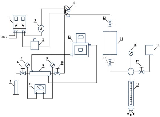
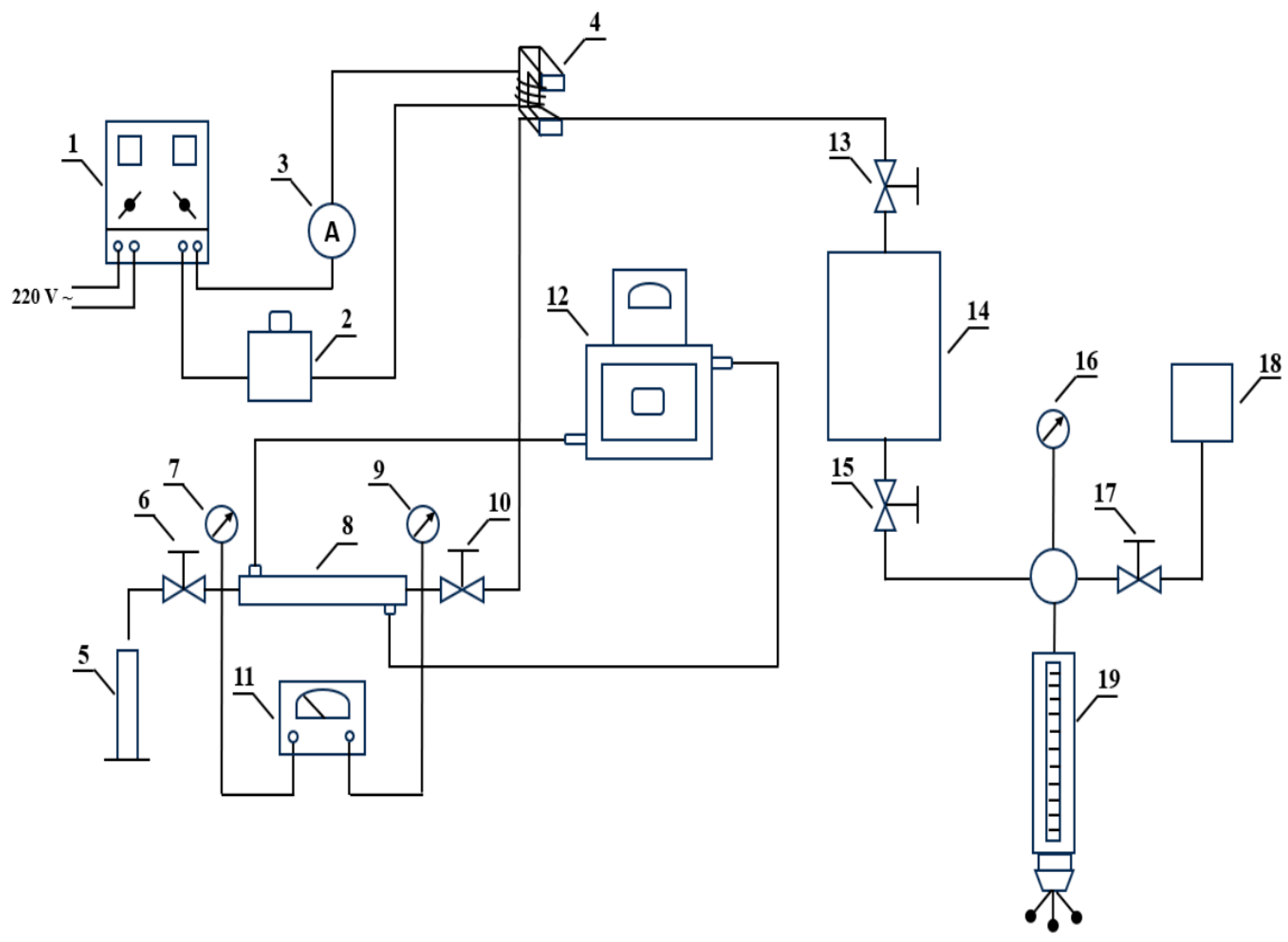
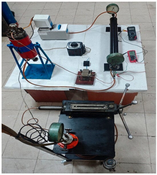
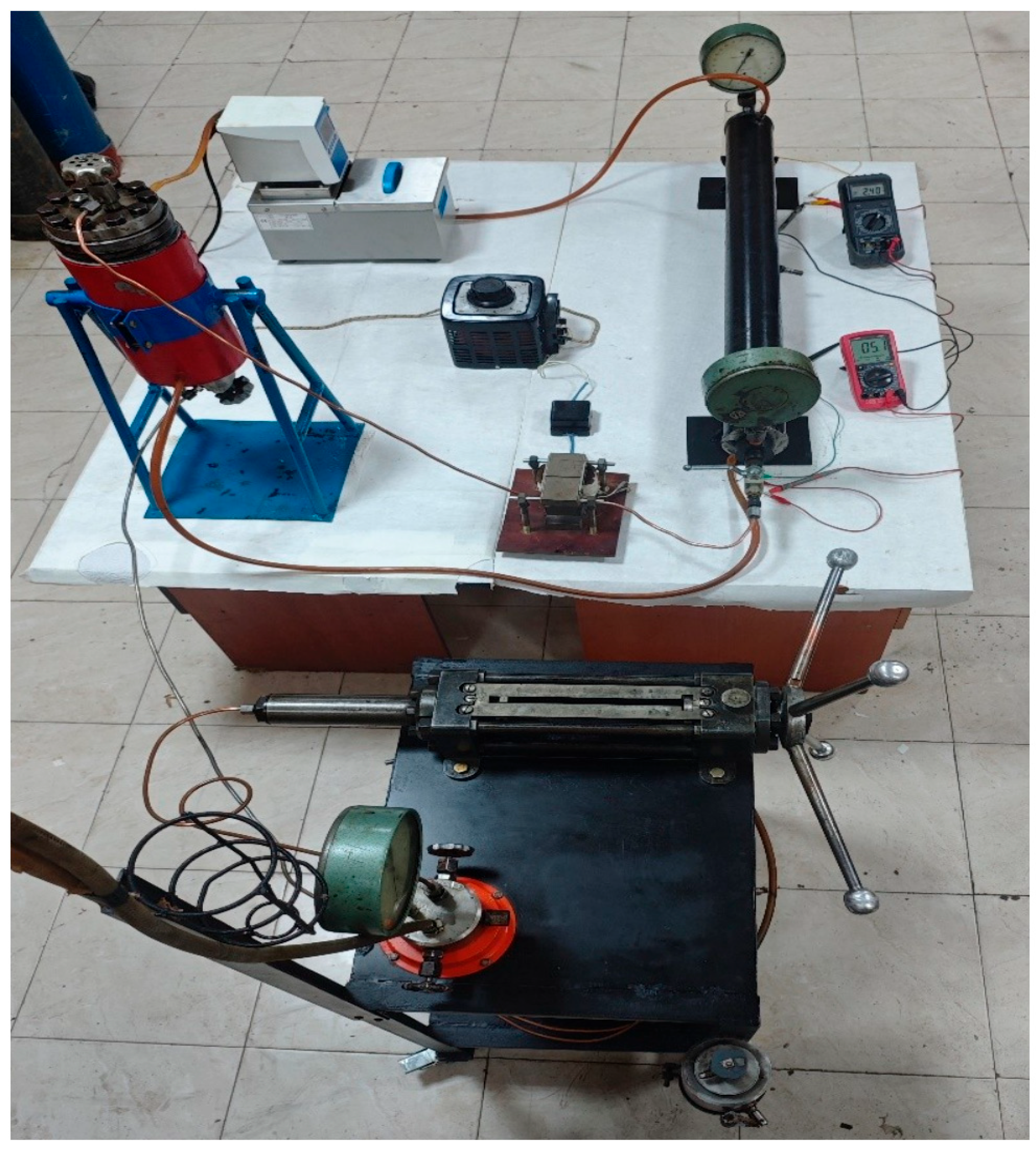
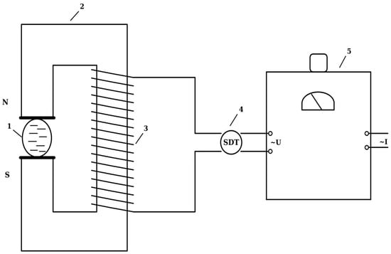
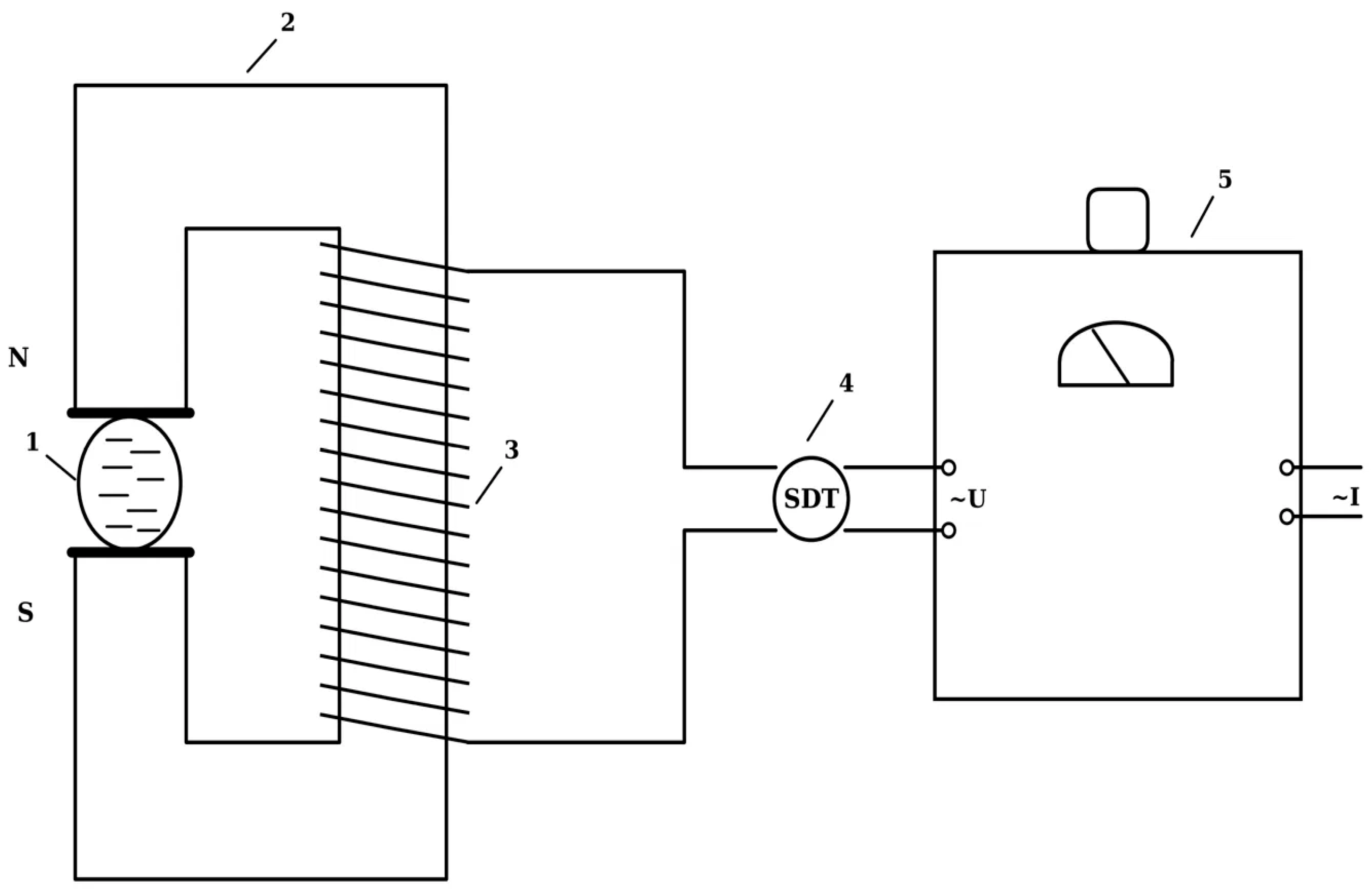
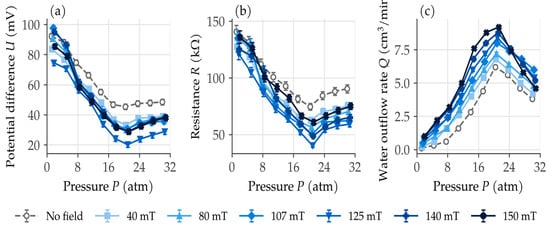
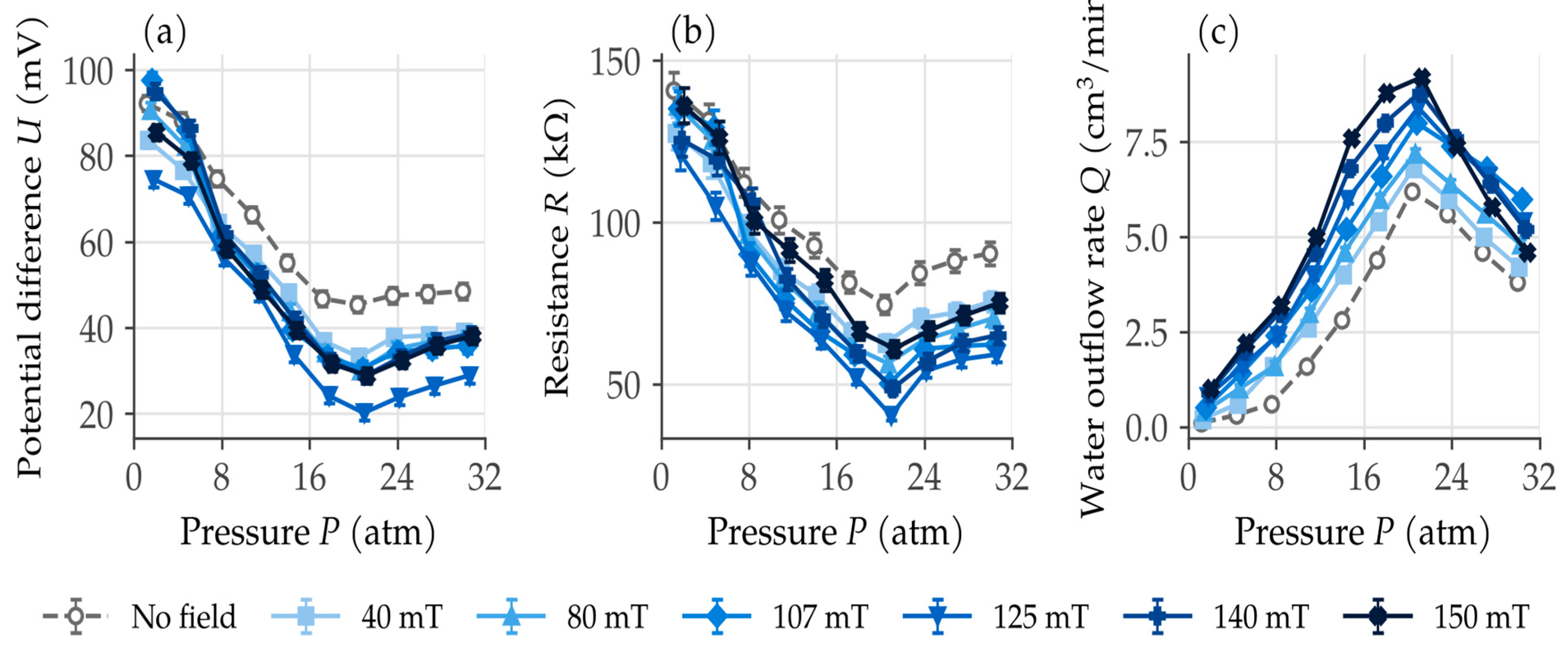
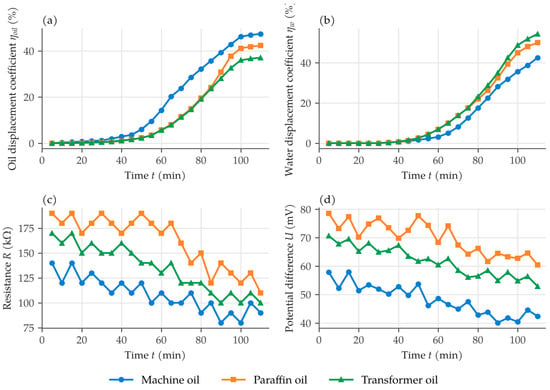
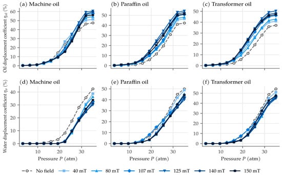
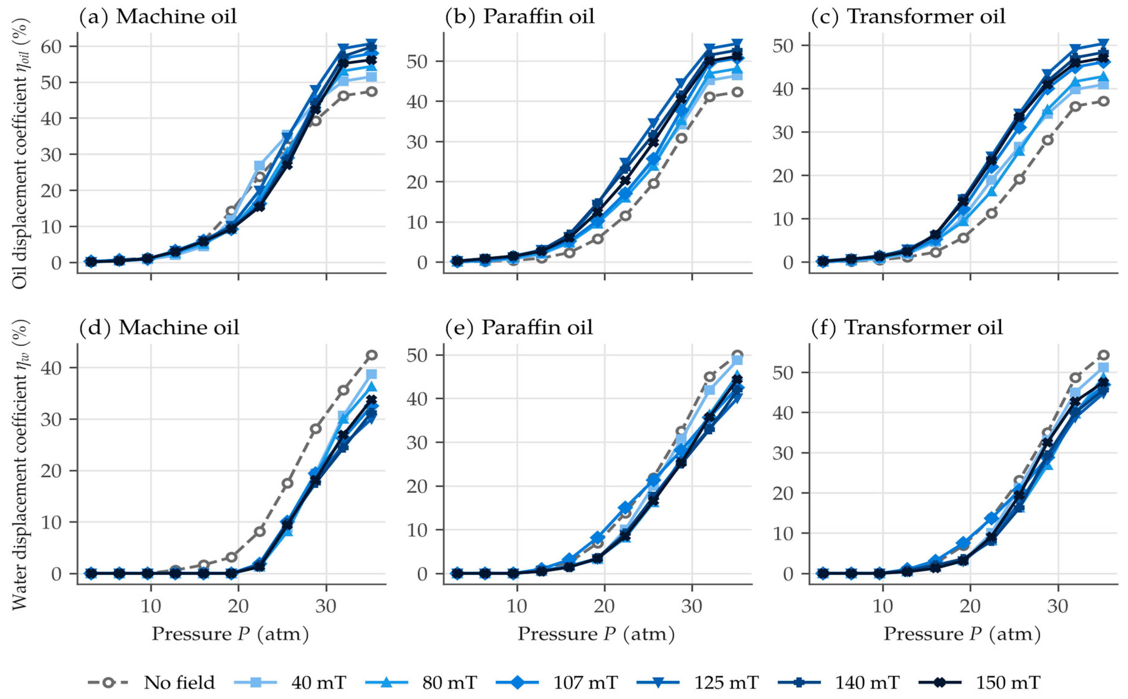
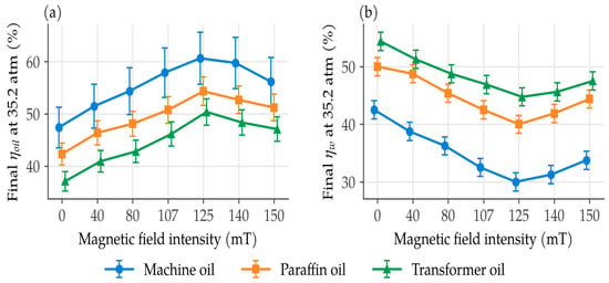

Disclaimer/Publisher’s Note: The statements, opinions and data contained in all publications are solely those of the individual author(s) and contributor(s) and not of MDPI and/or the editor(s). MDPI and/or the editor(s) disclaim responsibility for any injury to people or property resulting from any ideas, methods, instructions or products referred to in the content. |
© 2026 by the author. Licensee MDPI, Basel, Switzerland. This article is an open access article distributed under the terms and conditions of the Creative Commons Attribution (CC BY) license.