


Abstract
Cooling keeps even well-designed Saudi solar houses dependent on the grid. This study asks whether open-loop ground-coupled ventilation (GCV) can move a net-zero-energy Solar Decathlon house in Riyadh towards carbon-free operation. The house was re-modeled in Revit, Carrier HAP and HelioScope and validated against the original design. A buried vitrified clay pipe (19.8 m, 0.30 m diameter, 6 m deep) was sized with a regression-based design tool and coupled hour by hour to the outdoor air required by ASHRAE 62.2 (20 L s−1), with bypass control, calculated fan power and an hourly battery model. The pipe cooled the outdoor air by 4.8 K on average, yet saved only 2.8% of HVAC electricity (2.4% net of fan energy; 3.2% ahead of the house’s energy recovery exchanger), because ventilation is a small part of this envelope’s load; the saving reaches 32% only at 6.4 outdoor air changes per hour. Grid import (4961 kWh y−1, mostly at night) fell by 2.2% with GCV, by 23% with evening loads shifted to midday, and to 50–64 kWh y−1 with a 40 kWh battery and load shifting. The GCV has a negative net present value at current tariffs. Storage and demand scheduling, not cooling load, are the binding constraints.
1. Introduction
Saudi Arabia consumes more electricity per capita than almost any other country of comparable income, and the residential sector is responsible for roughly half of national consumption. Space cooling is the dominant end use within that sector; recent projections place cooling at about 65% of residential electricity use and indicate that residential demand could nearly double by 2060 if efficiency measures are not deployed at scale [1]. Any credible pathway to the Kingdom’s net-zero commitment and to the renewable energy targets of Vision 2030 therefore has to address residential cooling directly, not merely add generation capacity behind an unreformed load.
Two families of measures are available. The first reduces the load through envelope design, glazing, orientation and thermal mass; recent studies of Saudi dwellings show that envelope and passive measures can cut cooling or total energy use by roughly 40–70%, with insulation among the most effective single measures [2,3,4]. The second supplies the residual demand from renewable sources, most commonly rooftop photovoltaics, whose economics in the Kingdom have been examined for houses, mosques and other buildings [5,6,7,8]. The combination of the two defines the net-zero-energy home. Definitions of net-zero energy and net-zero carbon buildings differ in their balance boundary and metric, and the choice changes the emissions that are actually avoided [9,10]. In hot arid climates the concept is harder to satisfy, because the cooling peak coincides only partially with the solar peak and persists well after sunset.
A third family of measures sits between the two, namely, pre-conditioning ventilation air by passing it through buried pipes, variously described as a ground-coupled ventilation (GCV) system, an earth–air heat exchanger (EAHE) or an earth-to-air heat exchanger. Below a few meters, soil temperature in Riyadh remains close to the annual mean air temperature and far below summer ambient air, so outdoor air can be cooled sensibly before it reaches the cooling coil at the cost only of fan power. Recent reviews document the design variables that govern performance—pipe length, diameter, burial depth, air velocity, soil thermal properties and pipe material—and the wide range of reported performance [11,12,13,14,15]. In hot arid and semi-arid climates, experimental and numerical studies in Morocco, Algeria and Egypt report air temperature drops of up to about 19 K across long pipes [16,17,18], and work in Algeria and India has shown that soil thermal saturation under continuous operation can derate performance substantially unless the soil is allowed to recover [17,19,20]. Studies that express the benefit at the level of the installation or the building report much smaller figures: a 1.25–3.97% reduction in annual cooling load for EAHE configurations in a residential building in Kerman, Iran [21], and an annual output of the order of 250 kWh for a single EAHE in southern Algeria [22]. Within Saudi Arabia, earth tubes have been evaluated alongside natural ventilation and evaporative cooling for a prototypical villa [23], the contribution of EAHEs to heating and cooling loads has been mapped across six climatic zones [24], ground-source heat pumps have been assessed techno-economically [25,26], and a geothermal heat pump combined with photovoltaic–thermal collectors brought an arid residential building close to net-zero energy [27]. What is missing is an assessment of the simpler, non-refrigerant, open-loop ventilation variant in a real, constructed, high-performance Saudi solar house, coupled to the outdoor-air flow that the house actually requires and to its storage.
This paper supplies that assessment. The case study is the solar house designed and built by Team King Saud University for the 2018 Solar Decathlon Middle East in Dubai. The house reached net-zero energy on an annual balance but continued to import electricity from the grid at night, when battery storage was insufficient to carry the cooling load. It is, in other words, a building that has already exhausted the conventional envelope-plus-PV toolkit, and still falls short of carbon-free operation. The question addressed here is whether adding a ground-coupled ventilation system closes the remaining gap.
The specific objectives are as follows: (i) to re-model and validate the house under Riyadh rather than Dubai weather; (ii) to design a GCV configuration for Riyadh soil and climate conditions with a regression-based design tool and to check it independently; (iii) to quantify, at hourly resolution and at the outdoor-air rate required by ASHRAE Standard 62.2 [28], the resulting change in cooling and total electrical demand, including fan energy and the effect of bypass control; (iv) to determine, with a state-of-charge battery model, whether the reduced demand can be met by the existing photovoltaic and battery system, and how much storage and demand shifting carbon-free operation would require; and (v) to evaluate the intervention with discounted life-cycle indicators under the prevailing Saudi residential tariffs.
The contribution is threefold. To the authors’ knowledge this is the first hourly assessment of a ground-coupled ventilation system for a zero-energy house in Riyadh in which the ground loop is coupled to the code-required outdoor-air flow rather than to the supply-air flow of the air-handling unit, and it shows how strongly the apparent benefit depends on that choice; it quantifies the ceiling on what ventilation-side pre-cooling can achieve in an already optimized envelope; and it identifies, through an explicit hourly energy balance with a state-of-charge battery model, the constraints that actually bind when a net-zero-energy house is pushed towards carbon-free operation. Relative to the MSc thesis from which the work is drawn [29], the paper corrects the airflow used to couple the ground loop to the house, adds bypass control, a pressure-drop fan model, the space-heating hours and the energy-recovery exchanger of the house as designed, and an analytical check of the design tool, replaces a daily battery allowance with an hourly state-of-charge model, adds storage and demand-shifting scenarios, and replaces simple payback with net present value and the levelized cost of saved electricity.
2. Materials and Methods
2.1. Overview of the Workflow
The study is a quantitative, simulation-based assessment organized in seven sequential stages (Figure 1). Meteorological, ground-temperature and site data for Riyadh were assembled first; the building was then re-modeled and validated against the original design documentation; a GCV configuration was designed with the design tool and checked with an independent analytical model; its outlet air temperature was coupled hour by hour to the outdoor-air flow required by the house, with bypass control and fan energy; the resulting demand was set against on-site generation in an hourly energy balance with a state-of-charge battery model, including storage and demand-shifting scenarios; and finally operational carbon and life-cycle economics were evaluated. No physical experiment was carried out—the study is a design and simulation exercise, and the ground-coupled system was not built. The building model, the design-tool runs and a review of the literature are reported in the first author’s MSc thesis [29]; the coupling, energy-balance, carbon and economic results presented here were recomputed from the hourly simulation output of that work, as described in Section 2.5, Section 2.6 and Section 2.7.
2.2. Case-Study Building
The case-study building is a single-storey, single-family house of 81 m2 conditioned floor area and 3.30 m overall height, designed and constructed by Team King Saud University for the 2018 Solar Decathlon Middle East. It is arranged in a U-plan around a central courtyard, with the principal openings and transparent screens facing north following a sun-path analysis that identified the northern exposure as the lowest heat-gain orientation in Riyadh. Shading louvres protect the southern wall and vertical vegetation covers the western wall as an additional insulating layer. The plan is divided into four zones—public terrace and front garden, semi-public living room and office, service area, and private bedroom—with wet services grouped to minimize pipe runs (Figure 2).
Figure 2.
Ground-floor plan of the case-study solar house (drawing by the authors). Numbers in red circles identify the rooms listed in the legend; the other tags mark plumbing fixtures and appliances.
The structural system is a bolted steel frame in three transportable segments, with voided lightweight gypsum wall panels and autoclaved aerated concrete floor plates. Envelope construction and thermal resistances are summarized in Table 1. The house is occupied by two permanent residents and receives six visitors for dinner from 17:00 to 21:00. Summer indoor design conditions were 24.0 °C dry-bulb and approximately 50% relative humidity, and appliance usage factors were taken from the ASHRAE Handbook—Fundamentals [30].
Table 1.
Envelope construction and thermal resistance of the case-study house.
2.3. Simulation Tools and Model Validation
Four software tools were used. The building geometry, envelope layers and thermal properties were rebuilt in Autodesk Revit (Autodesk Inc., San Francisco, CA, USA) [31] from the project documentation, retaining only those elements that were actually constructed. Cooling and heating loads were computed hour by hour in the Carrier Hourly Analysis Program (HAP, version 4.90; Carrier Global Corporation, Pal Beach Gardens, FL, USA) [32], the same tool used by the original design team, so that the two models could be compared on identical terms. Photovoltaic generation was simulated in HelioScope (Aurora Solar Inc., San Francisco, CA, USA) [33] using the array as specified in the team’s design documentation [34]: 48 modules of 300 W (Aleo P19-300; aleo solar GmbH, Prenzlau, Germany) at 7° tilt and 180° azimuth feeding inverters limited to 8.0 kW AC, with a further 12 modules on the direct-current side charging a 14.4 kWh battery bank through a 2.5 kW charger. The final competition documentation lists 60 modules of 290 W (GIE-M60/290, Gree, Zhuhai, China; 17.4 kWp) with an expected annual yield of 25,280 kWh [34]; the design-stage specification was retained here because it is the one for which the team’s hourly energy balance was reported. The ground-coupled system was sized with the GCV evaluation tool, a MATLAB (The MathWorks Inc., Natick, MA, USA) [35] application that predicts outlet air temperature from regression models calibrated against measured data [36]. The simulation inputs and operating conditions are summarized in Table 2.
Table 2.
Simulation inputs and operating conditions.
Table 3.
Parameters of the ground-coupled ventilation system for Riyadh.
Validation proceeded in two steps. First, the re-modeled house was run under the Dubai weather file used by the original competition design so that the two peak-load calculations could be compared directly; the agreement is reported in Section 3.1. Second, annual on-site generation from the HelioScope model, with the documented daily battery contribution added, was compared with the yield reported by the original electrical team on the same basis. Only after both comparisons were judged acceptable was the weather file switched to Riyadh and the ground-coupled system introduced.
2.4. Design of the Ground-Coupled Ventilation System
A Riyadh typical meteorological year (TMY) file was imported into the GCV tool, supplying hourly ambient air temperature, together with ground temperatures at 2 m, 4 m and 6 m depth measured in situ in Riyadh by the tool’s author from January to December 2016 [36]. Design variables were then bounded—pipe length, burial depth, pipe diameter, soil type (clay, limestone or sand), number of parallel pipes, and volumetric flow rate—and the tool enumerated the admissible combinations [29]. For each candidate and each hour, the tool determines the operating mode by comparing inlet air temperature with ground temperature, predicts the outlet temperature from the regression models, computes the temperature change, and integrates the delivered energy over the year. Candidates were ranked by cumulative inlet-to-outlet temperature difference across the year, and the pipe geometry adopted was selected from the leading candidates as the one combining a high cumulative temperature difference with a pipe diameter and air velocity that are practicable for a residential installation: a vitrified clay pipe 19.8 m long and 0.30 m in diameter, buried 6.0 m deep in limestone, evaluated by the tool at 2.61 m3 min−1 (43.5 L s−1, 0.62 m s−1) per pipe. Its parameters are given in Table 3, its annual output in Table 4, and its predicted hourly performance in Figure 3.
Table 4.
Annual output of the selected pipe as computed by the design tool, and the cooling and heating delivered in the hourly energy balance at 20 L s−1.
Figure 3.
Predicted performance of the selected pipe over the Riyadh typical meteorological year at the tool design point: inlet (ambient) air temperature, outlet air temperature and undisturbed ground temperature at 6 m depth. Lines are daily means; bands show the daily range. Computed with the GCV evaluation tool [36].
The flow rate at which the ground loop is coupled to the house requires care. In the thesis, ten pipes of this geometry were specified so that the loop would carry 26.1 m3 min−1 (435 L s−1), the peak supply-air flow of the air-handling unit in the HAP model [29]. A ground loop can only pre-condition air that is drawn from outdoors, however, and the supply air of a recirculating air-handling unit is mostly return air at room temperature. The relevant flow is therefore the outdoor-air requirement of the house. For a dwelling of 81 m2 with one bedroom, ASHRAE Standard 62.2 requires 0.15 L s−1 m−2 × 81 m2 + 3.5 L s−1 × (1 + 1) = 19.2 L s−1 of whole-dwelling ventilation [28], taken here as 20 L s−1, or about 0.3 air changes per hour. A single pipe of the selected geometry carries this flow at 0.28 m s−1. Its outlet temperature was taken from the tool at the per-pipe design point; because the effectiveness of a buried pipe rises as the velocity falls, this is conservative, and an analytical estimate for 20 L s−1 is reported as an upper bound. The ten-pipe loop of the thesis is retained only for comparison, in the ventilation-rate sensitivity of Section 3.4 and the costs of Section 3.7.
A distinction should be noted between the pipe and the ground. The design tool models the thermal properties of the surrounding soil, which for the selected configuration was limestone; the pipe itself is a separate vitrified clay product, whose wall conductivity of 1.6 W m−1 K−1 was supplied as a design input. Vitrified clay pipes were chosen because it is chemically inert and durable when buried, has a smooth glazed bore that can be inspected and cleaned, is produced in the Kingdom for sewer applications, and conducts heat several times more effectively than the plastic pipes common in EAHEs. Pipe material is nevertheless a secondary variable, because the thermal resistance between the air and the undisturbed ground is dominated by internal convection and by the soil: a comparison of PVC, steel and copper pipes found a difference of only about 0.1 K in outlet temperature [18]. The tool reports delivered energy in thermal units, as the sensible heat removed from (or added to) the air stream; the conversion to electricity is described in Section 2.5.
Three checks were made on the applicability of the tool to Riyadh. First, the regression models were developed by the tool’s author and validated against the measured outlet temperatures of the ground-coupled ventilation system of the Solar CM House at Virginia Tech, on days in different seasons, and against computational fluid dynamics and GAEA simulations [36]; that installation is in a different climate and soil, so the use of the models for limestone under Riyadh’s conditions is an extrapolation. An independent steady-state effectiveness–NTU estimate was therefore made for one pipe, with internal convection from the Dittus–Boelter correlation and conduction through a 25 mm clay wall and through limestone (k = 2.0 W m−1 K−1) to a disturbed radius of 1.0 m. At the tool’s design point it gives an effectiveness of 0.54 (NTU = 0.78) against a median of 0.59 implied by the tool’s hourly output in cooling mode, so the tool agrees with a deliberately conservative analytical model to within about 10%; at 20 L s−1, the analytical effectiveness rises to 0.65. Second, the ground temperatures are measured rather than modeled: they were monitored in situ in Riyadh at 2, 4 and 6 m over the whole of 2016 by the tool’s author, who also used them to design a ground-coupled ventilation system for an office building in the city [36]. At 6 m they range from 23.3 to 27.5 °C (mean 25.4 °C), and they are consistent with conduction theory: the Kusuda–Achenbach model [39], driven by the air temperature record of the weather file (mean 25.7 °C, annual amplitude 10.2 K) with a thermal diffusivity of 1.5 × 10⁻⁶ m2 s−1, typical of limestone, reproduces them to within 0.34 K root-mean-square, including the lag of the minimum to April. Third, the tool treats the ground as undisturbed. Continuous operation warms the soil around a pipe and can derate its cooling by a third or more [17,40], and closely spaced parallel pipes interfere: in a recent analysis the cooling capacity of the middle pipe of three fell by 19% at 1.0 m spacing and by 5% at 2.0 m, about 3 m being required in soil of 2 W m−1 K−1 [41]. For the single pipe adopted here the heat rejected to the ground is modest (534 kWh y−1, at most about 15 W per meter of pipe), the bypass control interrupts operation whenever the ground is warmer than the air, which allows the soil to recover [17,42], and no interference arises. For the ten-pipe layout of the sensitivity analysis the derating would be significant, and its costs in Section 3.7 are given for 1 m and 3 m spacing.
2.5. Coupling and Energy Balance
The hourly outlet air temperature predicted by the GCV tool was coupled to the HAP results of the house as follows. In every hour in which the outlet air was cooler than the outdoor air and the house required cooling, the outdoor air was routed through the ground loop and the sensible cooling it delivered was computed as Q = ρcpVoa(Tamb − Tout), with ρcp = 1.207 kJ m−3 K−1 and Voa = 20 L s−1. This thermal quantity was converted to electricity using the coefficient of performance of the cooling plant in the same hour, obtained as the ratio of the cooling coil load to the HVAC electricity in the design team’s HAP design-day performance for that hour (mean 2.32 over the hours with a cooling load, and 2.22 on an annual energy basis), and subtracted from the cooling electricity of that hour, never exceeding the coil load of the hour. The hourly HAP results also contain space heating; 920 kWh y−1 between November and March, in 1235 h, with a peak of 2.0 kW and 87% of the energy between 17:00 and 07:00, met in the model by electric terminal heaters whose input equals the load. This heating was not part of the design team’s electricity profile and has been added to the baseline here. In the 360 h in which the house needs heating and no cooling, the outlet air of the loop is warmer than the outdoor air, and the loop pre-heats the ventilation air; the heat it delivers, Q = ρcpVoa(Tout − Tamb) capped at the heating load of the hour, is credited one-for-one as electricity. In the other 875 heating hours HAP also reports a cooling coil load, because the variable-air-volume system cools the supply air and reheats it at the terminal; pre-heating the outdoor air would then add to the coil load, and the loop is bypassed. In all other hours a damper bypasses the loop, the outdoor air enters directly as in the baseline, and the ground-loop fan is off. The bypass matters because the outlet air is warmer than the outdoor air in 4137 h of the year, and in 3757 of those hours the house needs cooling, so operation without a bypass would warm the ventilation air against the load. Both cases are reported in Section 3.4.
The outdoor air contained in the HAP baseline was checked against the design report and the hourly results. As designed, the house takes in 112–149 L s−1 of outdoor air through a total-energy exchanger that recovers heat from the kitchen and bathroom exhaust before the fresh air is mixed with return air at the air-handling unit [29]. At the Riyadh cooling design condition, HAP reports a ventilation load of 553 W for 112 L s−1 at 42.3 °C [29], which implies a sensible effectiveness of about 0.78 and equals the load of only 25 L s−1 of untreated outdoor air; at the heating design condition it reports 1353 W for 149 L s−1 at 5.0 °C, an effectiveness of about 0.53. The hourly results agree: regressed against outdoor temperature, the baseline coil load rises by 0.12 kW K−1 at night and by 0.17 kW K−1 on a daily mean basis, where solar gains also correlate with temperature, against an envelope conductance of 0.12 kW K−1 implied by the HAP design report [34], whereas 435 L s−1 of untreated outdoor air would on its own add 0.53 kW K−1. The outdoor air that reaches the coil in the baseline is therefore equivalent to about the ASHRAE 62.2 rate, and coupling the loop at 435 L s−1 would credit it with cooling outdoor air that the baseline house never had to cool. Two variants are evaluated in Section 3.4. For the sensitivity to the ventilation rate, the baseline coil load was adjusted hour by hour by ρcp(V − 20 L s−1)(Tamb − 24 °C) for an untreated outdoor-air flow V, and the heating load of the heating-only hours by ρcp(V − 20 L s−1)(21.1 °C − Tamb), so that the baseline and the ground loop always carry the same outdoor air. For the house as designed, the loop carries the full 149 L s−1 ahead of the total-energy exchanger; the HAP baseline is then left unchanged, and only the fraction 1 − ε of the temperature change produced by the loop reaches the coil, with ε = 0.78 in cooling and 0.53 in heating. Latent loads were not adjusted, because Riyadh outdoor air is drier than the indoor air (Section 3.1).
Fan energy was calculated rather than bounded. The pressure drop of the ground-loop path comprises friction in the 19.8 m horizontal pipe and two 6.3 m risers (Darcy–Weisbach, with the Colebrook friction factor and an absolute roughness of 0.5 mm), minor losses at the entry, four bends and the exit (K = 2.7, plus 1.0 for manifolds where there are several pipes), an intake hood with sand screen (25 Pa), a coarse inlet filter (100 Pa, the mean of the clean and loaded values) and connecting ductwork (10–20 Pa). Fan electrical power is the product of flow and pressure drop divided by an overall fan–motor efficiency of 0.30 for the single small fan, 0.40 for four pipes and 0.45 for the ten-pipe loop, and the fan runs only when the loop is in use. The HAP HVAC electricity already includes the supply fan of the air-handling unit, which moves the same air in the baseline, so the ground-loop fan is the only additional fan and is not double-counted.
The energy balance set household demand against on-site generation and storage hour by hour, using a state-of-charge model of the system as designed [34]. The 48-module array supplies the house through inverters limited to 8.0 kW AC, as simulated in HelioScope. The 12-module sub-array, assumed to share the orientation of the main array and therefore to produce one quarter of its output (5734 kWh y−1), feeds a DC-coupled charger that charges the 14.4 kWh battery at up to 2.5 kW and passes the remainder to the inverters when they have spare capacity; output that can be neither stored nor inverted is curtailed. The battery discharges at up to 2.5 kW whenever demand exceeds direct supply, between 15% and 100% state of charge, with a round-trip efficiency of 85% for the lead-acid bank. Remaining deficits are imported from the grid and remaining surpluses exported. The year was simulated twice in succession and the second year reported, so that the result does not depend on the initial state of charge. In this model the battery stores photovoltaic energy, with losses; it is not counted as generation. Appliance loads were held at the constant daily schedule of the original design and the envelope, array and battery at their design values, so that the effect of the ground-coupled system could be isolated.
Two further scenarios test whether storage and the appliance schedule are the binding constraints. In the demand-shifting scenario, the appliance energy used between 19:00 and 24:00 above the base load (3.1 kWh d−1, including dish-washing at 21:00 in the design schedule [34]) is moved to 11:00–15:00. In the storage scenario, the battery is replaced by an AC-coupled lithium-ion battery of 0–60 kWh (10–100% state of charge, 92% round trip, power limit of 2.5 kW or half the capacity per hour, whichever is greater) that can be charged from any photovoltaic surplus. The house is described as carbon-free on a given day only when no grid electricity is imported in any hour of that day; self-sufficiency is defined as 1 − import/demand and self-consumption as 1 − (export + curtailment)/generation.
2.6. Operational Carbon Accounting
Because the research question is framed in carbon rather than energy, household electricity was converted to carbon dioxide using a grid emission factor. The Saudi electricity system remains almost entirely fossil-fueled—Ember reports a 98% fossil share and a 2% solar and wind share, with a regional power-sector intensity of 636 gCO2e kWh−1 for the Middle East in 2024 [37]. A central value of 0.65 kgCO2 kWh−1 was adopted, consistent with the baseline grid emission factor used in recent peer-reviewed work on Saudi decarbonization [38], and results are reported with a sensitivity band of 0.55 to 0.75 kgCO2 kWh−1.
Three conventions are reported side by side. Demand-side carbon values total household electricity at the grid emission factor, and answers the question of what the house would emit if its demand were met from the network. Net carbon values the net exchange with the grid, exports minus imports, at the same factor, and answers the question of what the installation does to system-wide emissions. Grid-import carbon values only the electricity actually purchased in the hourly balance. Because the study is concerned with a change in operation rather than with a whole life-cycle inventory, embodied carbon in the pipework, excavation and photovoltaic array is outside the present scope, and is identified in Section 4.4 as a limitation. A single annual factor is used rather than an hourly one; the justification, and the conditions under which that simplification would cease to hold are set out in Section 4.2.
2.7. Economic Analysis
Capital costs for the ground-coupled system were estimated from unit prices obtained in the Saudi local market for the thesis design [29]: 126 SAR m−1 for vitrified clay pipe (quoted for a 0.61 m pipe and therefore an upper bound for 0.30 m), 30 SAR m−3 for excavation and backfill in limestone, 6000 SAR for the filtered fan package and 5000 SAR for ducting and installation, applied to the quantities of the configuration actually analyzed. Prices are given in Saudi riyals (SAR) and in US dollars at the fixed exchange rate of 3.75 SAR per USD [43]. Operating savings were valued at the residential tariff approved by Council of Ministers’ decree and in force since 1 January 2018 and still applied in 2026, 0.18 SAR kWh−1 for monthly consumption up to 6000 kWh [44]. The second tier of 0.30 SAR kWh−1 above 6000 kWh is not reached by the case-study house, whose highest monthly consumption is about 2140 kWh. Exported electricity was valued at 0.07 SAR kWh−1, the credit for residential customers under the net-billing arrangement of the regulatory framework for small-scale solar photovoltaic systems [45]. The annual benefit B of the ground loop was taken from the hourly energy balance as the change in grid purchases valued at the tariff plus the change in exports valued at the export credit. Two indicators were computed over a 30-year analysis period, shorter than the life of buried pipework but longer than that of the fan, which is replaced once after 15 years: the net present value
and the levelized cost of saved electricity
where C0 is the capital cost, CRF = r(1 + r)N/[(1 + r)N − 1] the capital recovery factor, M = 500 SAR y−1 the maintenance cost, R = 6000 SAR the fan replacement, r the real discount rate (3%, 5% and 8%), N = 30 years and Es the net electricity saved per year. There is at present no incentive scheme for residential ground-coupled installations in the Kingdom, so no incentive term is included, and tariffs are held constant in real terms.
NPV = −C0 + Σt=1…N (B − M)/(1 + r)t − R/(1 + r)15,
LCSE = {[C0 + R/(1 + r)15] × CRF + M}/Es,
2.8. Use of Generative Artificial Intelligence
Generative AI (Claude, Opus model series; Anthropic PBC, San Francisco, CA, USA) was used during manuscript preparation to draft text from the first author’s thesis, to write and run the scripts that recompute the hourly coupling, fan, battery, carbon and economic results from the hourly simulation output, to draw the figures from that output, and to add the room legend, north arrow and scale bar to the authors’ plan drawing in Figure 2, and to search for and check references. The scripts “written in Python (version 3.13; Python Software Foundation, Wilmington, DE, USA)”, and the hourly energy-balance data are provided as Supplementary Materials so that every recomputed value can be reproduced. All recomputed values were checked against the simulation files by the authors. Generative AI was not used to generate or alter simulation input or output data.
3. Results
3.1. Model Validation
Table 5 compares peak design cooling loads from the original design team’s calculation [34] and the re-modeled house under identical Dubai weather. Total system sensible load differs by 125 W, or 2.3%, and the individual envelope components agree closely; the largest single discrepancy, in window and skylight solar gain, reflects the updated solar model in the more recent version of the calculation software rather than a difference in the building itself. Annual on-site generation from the HelioScope model was 27,318 kWh on the design team’s basis (22,938 kWh from the 48-module array plus the documented 12 kWh per day stored from the 12-module sub-array) against 26,261 kWh in the original team’s design documentation [34], a difference of 4.0%; against the 25,280 kWh expected for the modules finally installed, the difference is 8.1%, which reflects the change of module rather than the model. Both deviations are within the range normally accepted for independent re-modeling of the same building, and the re-modeled house was therefore adopted as the baseline. No metered energy data from the house in use were available to the authors, so the baseline could not be calibrated against measured consumption in the sense of ASHRAE Guideline 14 [46]; the validation is model-to-model, and Section 4.4 discusses the consequence.
Table 5.
Peak design cooling loads: original design calculation (data from [34]) versus re-modeled house (Dubai weather, July 17:00), and the re-modeled house under Riyadh weather.
Switching the weather file from Dubai to Riyadh moves the peak from 17:00 to 13:00 and raises the outdoor design dry-bulb temperature from 40.7 to 42.3 °C, while the coincident wet-bulb temperature falls from 23.6 to 17.3 °C. The sensible peak rises slightly (5703 W) and the design heating requirement is higher (3142 W against 2404 W), reflecting the colder and drier Riyadh winter; the hourly simulation accordingly contains a small space-heating demand (Section 2.5). The zero latent load in the Riyadh column does not mean that the occupants release no moisture. At the Riyadh design condition the outdoor air holds about 3.0 g of water vapor per kilogram of dry air, against 10.0 g kg−1 in the room at 24 °C and 50% relative humidity, so each liter per second of outdoor air removes about 21 W of latent heat; even at 20 L s−1 this is about 0.4 kW, more than the latent gains of the occupants, and HAP reports the net latent load of the system as zero because the coil cannot humidify. Figure 4 compares the cooling coil load of the two climates on the design day of each month: Riyadh requires less cooling than Dubai in every month, most markedly in winter. The figure is a thermal load on design days and is used only to compare the climates; no result below is derived from it.
3.2. Baseline Demand Structure
Figure 5 decomposes the baseline monthly demand into cooling, space-heating and appliance components. Appliance demand is constant by construction at 19.35 kWh d−1, whereas cooling electricity varies from 5.76 kWh d−1 in January to 49.69 kWh d−1 in July, and space heating adds up to 12.0 kWh d−1 in December and January. Over the year, HVAC accounts for 11,286 kWh of a total 18,349 kWh, or 61.5% of household electricity (10,366 kWh for cooling and 920 kWh for heating)—consistent with the national picture in which cooling dominates residential consumption [1]. This concentration is what makes a cooling-side intervention worth testing; more than half of the demand is addressable in principle.
Figure 4.
Cooling coil load of the re-modeled house under Dubai and Riyadh weather, summed over the 24 h of each month’s design day (thermal load; plotted from the HAP design-day output [29]).
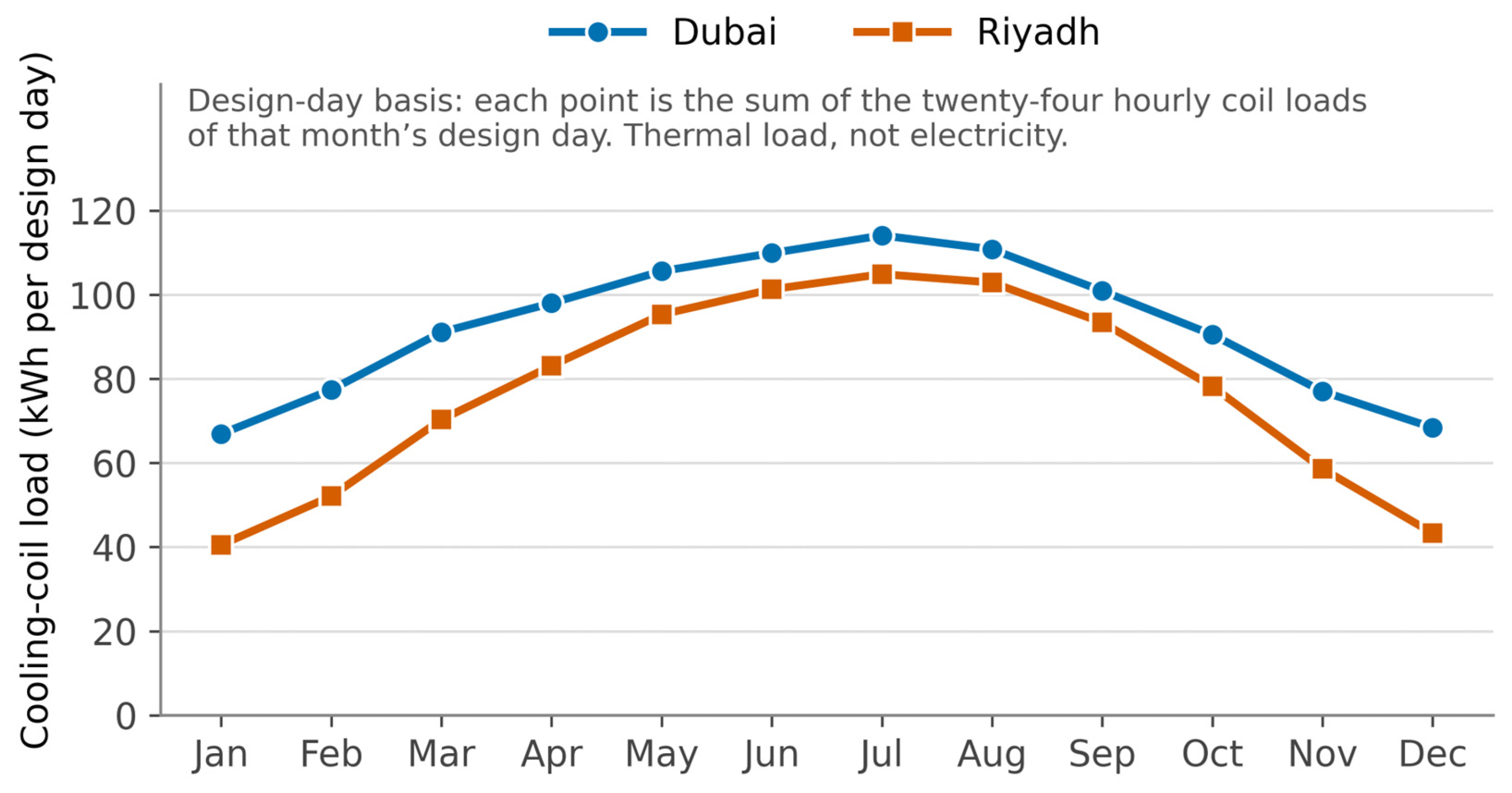
Figure 5.
Baseline monthly average daily electrical demand, split into cooling, space-heating and appliance components. Plotted from the hourly simulation output (Table 6).
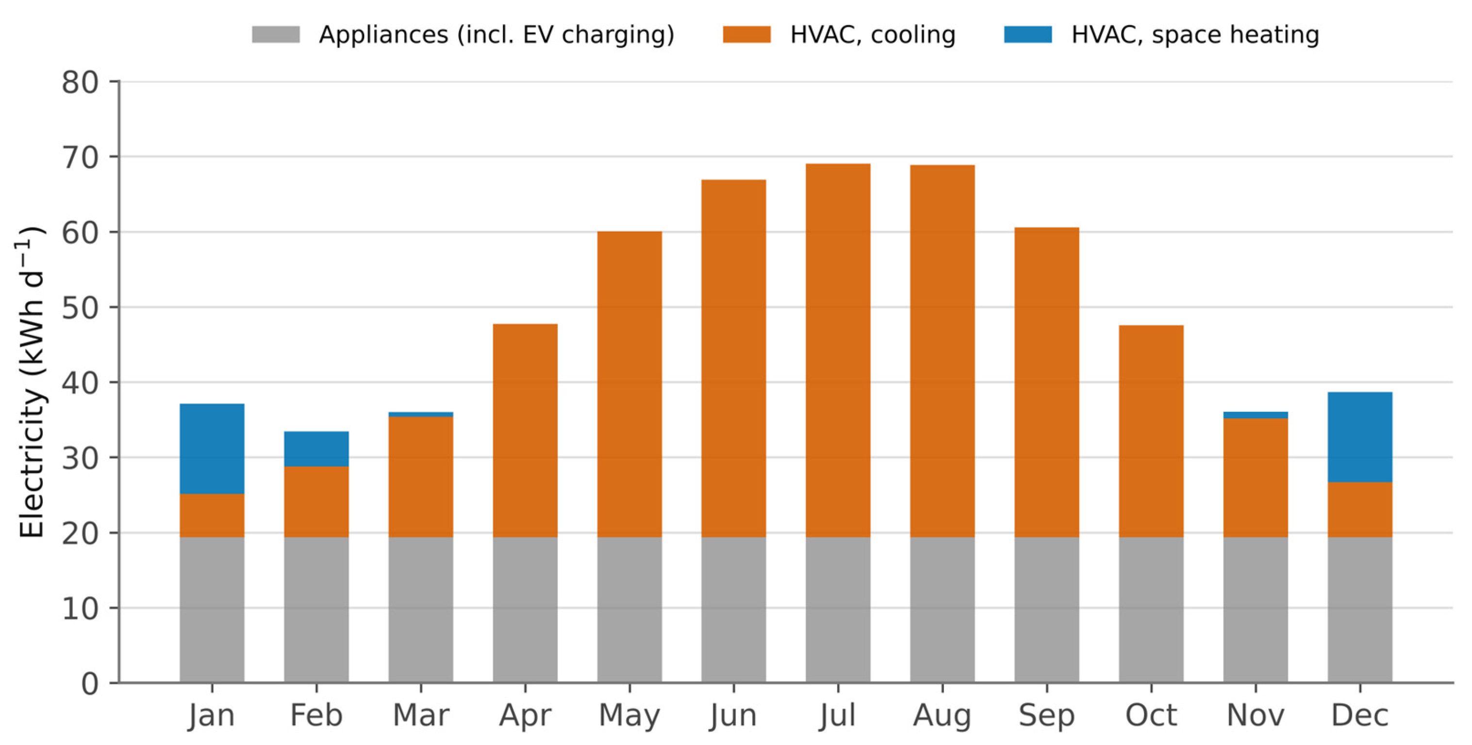
Table 6.
Monthly average daily electrical demand with and without the GCV system at 20 L s−1 (kWh d−1), from the hourly energy balance. HVAC values with GCV include the ground-loop fan.
3.3. Effect of the Ground-Coupled Ventilation System
Table 6 reports monthly average daily electrical demand before and after the ground loop is applied to the outdoor air, separately for total demand and for the HVAC component, the latter including the ground-loop fan. The pattern is seasonal and the magnitude small. From December to February the loop pre-heats the outdoor air in the hours that need heating and reduces HVAC electricity by 3.5–4.8%, or 0.5–0.9 kWh d−1; in March, October and November, when the outdoor air is close to the ground temperature, it delivers almost nothing. From April the cooling contribution grows, and it peaks in July, when average daily HVAC consumption falls from 49.69 to 48.22 kWh d−1, a reduction of 3.0%.
Summing the hourly values gives the annual totals in Table 7. The ground loop delivers 534 kWh y−1 of sensible cooling to the outdoor air, a mean temperature drop of 4.8 K over 4623 h, worth 247 kWh y−1 of HVAC electricity at the hourly plant efficiency, and 68 kWh y−1 of pre-heating in 360 heating hours (mean temperature rise 7.8 K), which displaces the same amount of electric heating. The fan consumes 45 kWh y−1, so the net reduction in HVAC electricity is 270 kWh y−1, or 2.4%, and total household electricity falls by 1.5%, from 18,349 to 18,079 kWh y−1; energy use intensity falls from 227 to 223 kWh m−2 y−1. If the lower velocity in the single pipe is credited through the analytical effectiveness of Section 2.4, the gross saving rises to 376 kWh y−1 and the net saving to 331 kWh y−1 (2.9%); conversely, with the coefficient of performance of HAP’s own plant model (seasonal 3.23) in place of the design team’s, the cooling part of the saving would fall from 247 to 174 kWh y−1. Neither changes the picture. The reason is structural. At 20 L s−1 the loop can remove at most 0.30 kW, even at its maximum temperature drop of 12.6 K, against a peak sensible cooling load of 5.7 kW (Table 5): in a house with walls of 5.36 m2 K W−1 thermal resistance, triple glazing and two permanent occupants, the outdoor air carries only a small part of the cooling load.
Table 7.
Annual electrical demand and energy use intensity, with and without the GCV system (20 L s−1, bypass control).
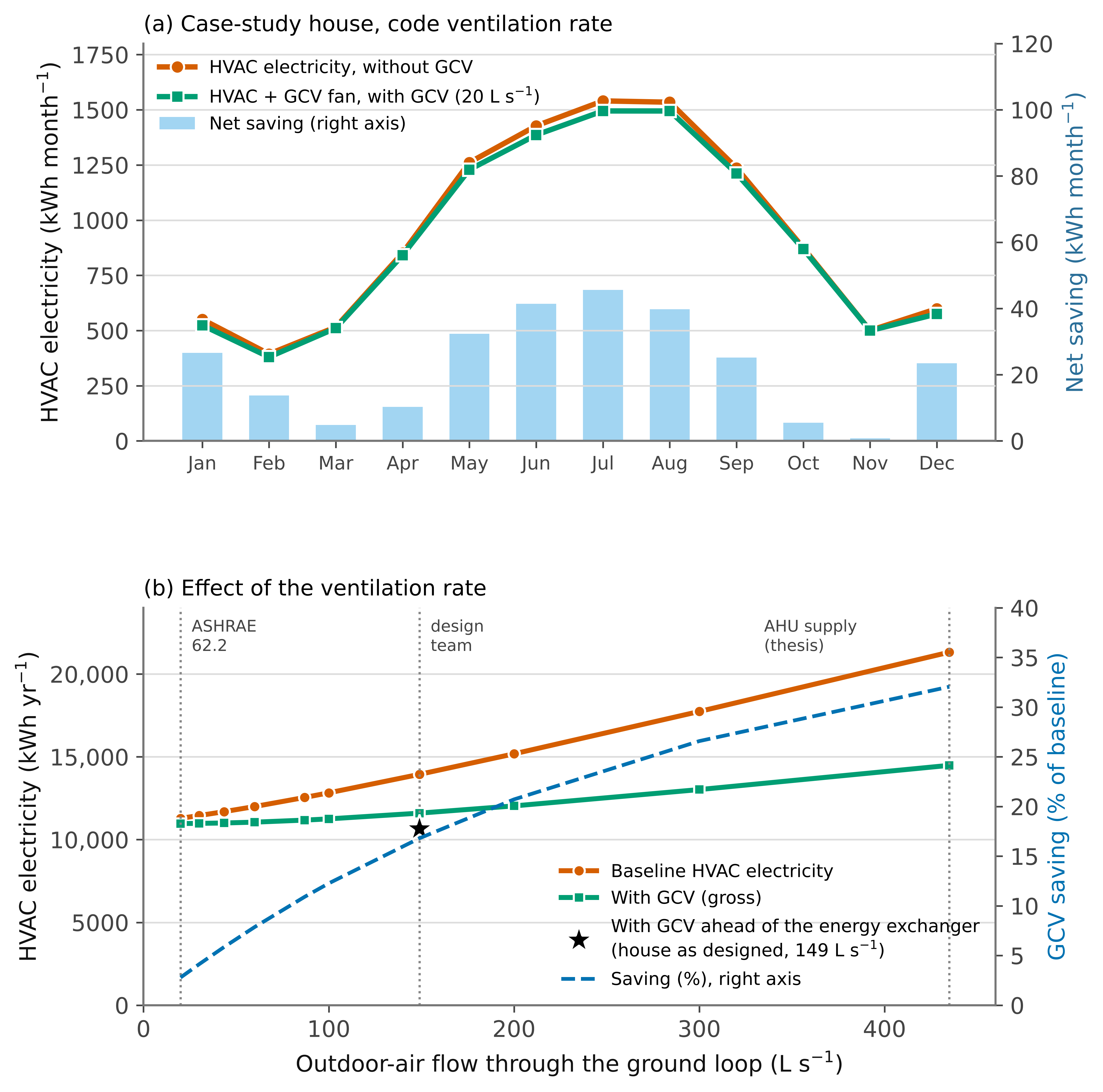
Figure 6a shows the same result as a seasonal profile. The two curves are almost indistinguishable; the largest monthly net saving is 46 kWh, in July, 3.0% of that month’s HVAC electricity, while pre-heating gives net savings of 27 and 24 kWh in January and December. Figure 6b places the result in the context of the variable that decides it, the outdoor-air flow carried by the loop, which is examined in Section 3.4.
Figure 6.
(a) Monthly HVAC electricity with and without the GCV system at the ASHRAE 62.2 outdoor-air rate, and the net monthly saving after fan energy; (b) annual HVAC electricity of the baseline and with the GCV system as a function of the outdoor-air flow carried by the loop, with the baseline adjusted to the same flow; the star marks the loop carrying 149 L s−1 ahead of the total-energy exchanger of the house as designed, with the HAP baseline unchanged.
3.4. Ventilation Rate, Bypass Control and Fan Energy
Table 8 sets out the gross saving, fan energy and net saving for four flows of untreated outdoor air—the ASHRAE 62.2 rate adopted here, one pipe at the tool’s design point, the 149 L s−1 specified by the original design team for the competition occupancy [34], and the 435 L s−1 supply-air flow to which the ten-pipe loop was sized in the thesis [29]—and for the house as designed. In the first four cases the baseline carries the same outdoor air. The saving rises almost in proportion to the flow, to 6834 kWh y−1 at 435 L s−1, but so does the baseline, which with 6.4 air changes per hour of untreated outdoor air would consume 21,320 kWh y−1 of HVAC electricity, 89% more than the house as modeled. Relative to a consistent baseline, the large loop would save 32% (29% net of fan energy), and it would do so only by conditioning outdoor air that the house does not need. The house as designed shows what an energy-recovery exchanger does to the case for a ground loop. Four pipes carrying the full 149 L s−1 ahead of the exchanger save 638 kWh y−1 gross, because the exchanger already recovers about 78% of the temperature difference that the loop would otherwise exploit in cooling (53% in heating); the fan for the larger flow consumes 271 kWh y−1, leaving 367 kWh y−1, or 3.2%. The reduction of about half that is obtained when the 435 L s−1 loop is set against the house as modeled is an artefact of coupling the loop to the supply-air flow.
Table 8.
Effect of the outdoor-air flow carried by the ground loop on the baseline, the saving and the fan energy (baseline adjusted to the same untreated outdoor-air flow except in the last row; bypass control unless stated).
The calculated fan power is small for the single pipe—9 W at a pressure drop of 135 Pa, of which only 0.3 Pa arises in the pipe itself, the intake and filter dominating at low velocity. Over the 4983 h of operation, the fan consumes 45 kWh y−1, 14% of the gross saving. For the ten-pipe loop the fan draws 142 W, consistent with the 0.19 kW nameplate motor specified in the thesis, and consumes 706 kWh y−1. Bypass control is essential in this climate. Without it the loop would run whenever the house needs cooling, including 3757 h in which its outlet air is warmer than the outdoor air; the resulting penalty of 152 kWh y−1 would cancel 62% of the gross cooling saving at 20 L s−1, and the additional fan hours would consume most of the remainder (Table 8).
For the case-study house, the conclusion is robust to every assumption in Table 8 that can be defended; at the outdoor-air rate the house requires, or with the outdoor air it actually takes in through its energy-recovery exchanger, the ground loop removes 2.4–3.2% of HVAC electricity net of fan energy. A ground loop of this kind earns its keep only where a building must take in large volumes of outdoor air.
3.5. Energy Balance and Zero-Carbon Status
Figure 7 sets monthly generation from all 60 design-stage modules (48 + 12 of 300 W) against monthly demand and grid import. Generation exceeds demand in every month and, by a wide margin, over the year (Table 9); on a daily basis, generation from all 60 modules falls short of demand on 13 days of low solar output, with or without the ground loop, which narrows the shortfall on those days but does not remove it. The ground loop changes demand very little: in July, the month of greatest benefit, monthly demand falls by 46 kWh.
Table 9.
Hourly energy balance with the 14.4 kWh battery as designed (state-of-charge model), with and without the GCV system, and with evening appliance loads shifted to midday.
Carbon-free operation in the strict sense was not attained in any configuration of the house as designed. Generation and demand do not coincide in time (Figure 8); the array produces its surplus between mid-morning and late afternoon, while cooling and appliance loads persist into the evening and the night. The 14.4 kWh battery, charged only from the 12-module sub-array and limited to 2.5 kW, delivers on average 11.1 kWh d−1—close to the 12 kWh d−1 assumed by the design team—but cannot carry the evening peak and the night. The house imports 4961 kWh y−1, 99.6% of it between 17:00 and 07:00, and does so on every day of the year; self-sufficiency is 73%, while 14,328 kWh y−1 is exported (Table 9). The ground loop reduces grid purchases by 111 kWh y−1 (2.2%) and raises exports by 158 kWh y−1, because most of the electricity it saves in the cooling season would otherwise have been supplied by the array, whereas its winter pre-heating acts mainly on night-time heating and therefore on purchases. By contrast, moving 3.1 kWh d−1 of evening appliance use to midday reduces grid purchases by 23%, about ten times as much as the ground loop.
Figure 7.
Monthly photovoltaic generation (60 modules), electrical demand, and grid import with the battery as designed, with and without the ground-coupled ventilation system.
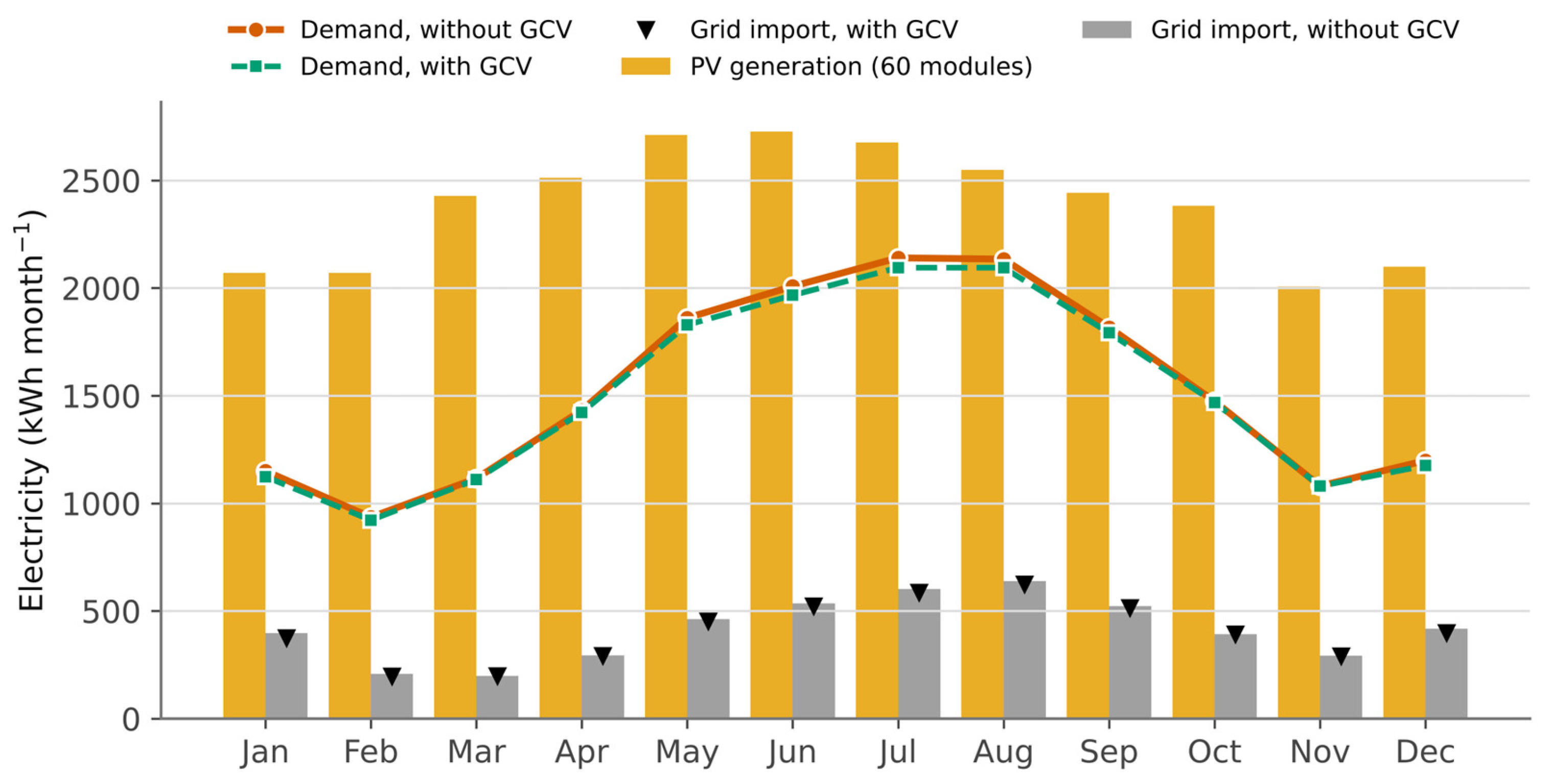
Figure 8.
Mean July day: photovoltaic generation from all 60 modules, household demand without and with the GCV system and with evening loads shifted to midday, and grid import with the battery as designed. The ground loop changes demand very little; the evening and night-time demand that forces grid import is a matter of storage and scheduling.
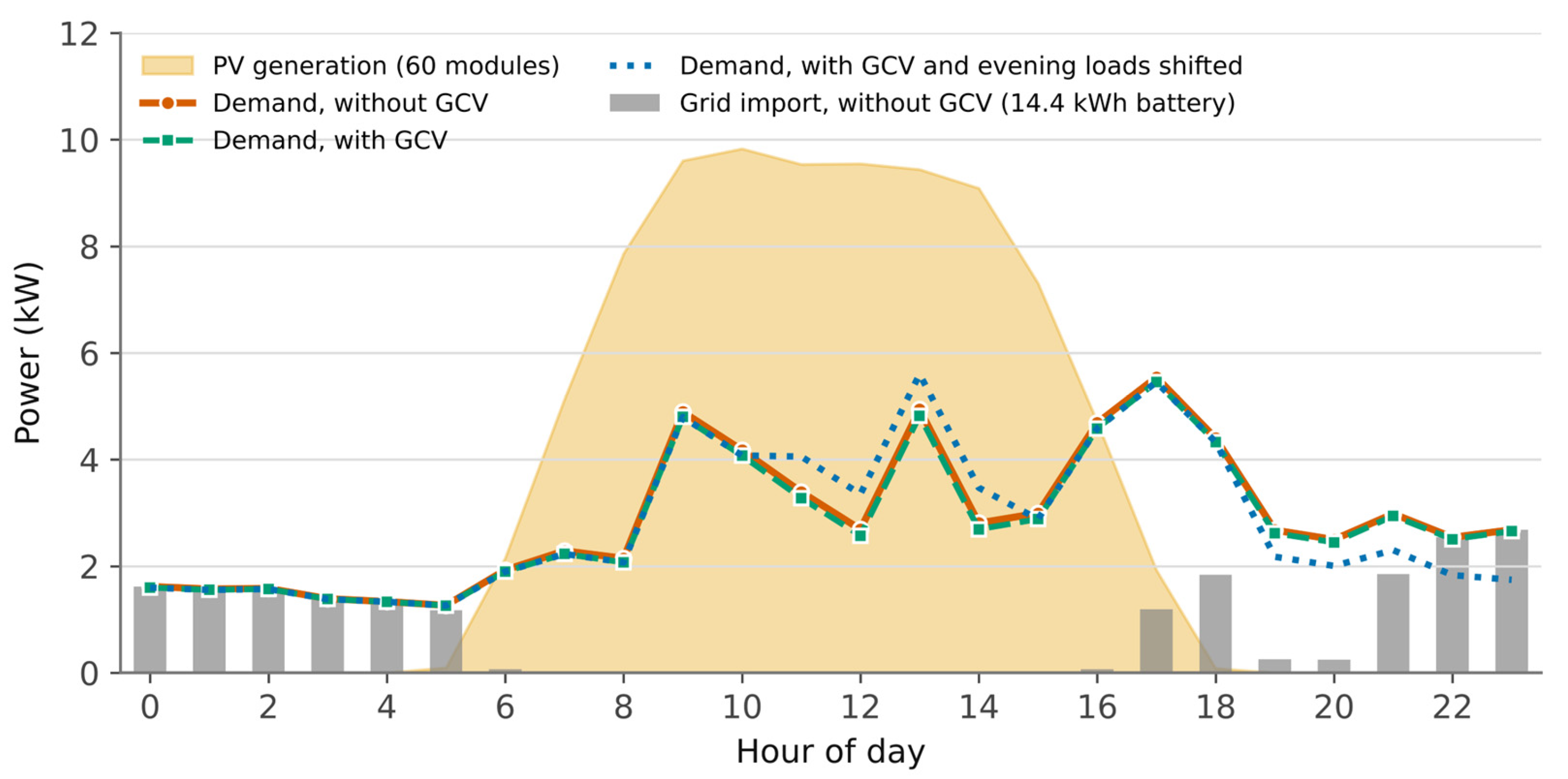
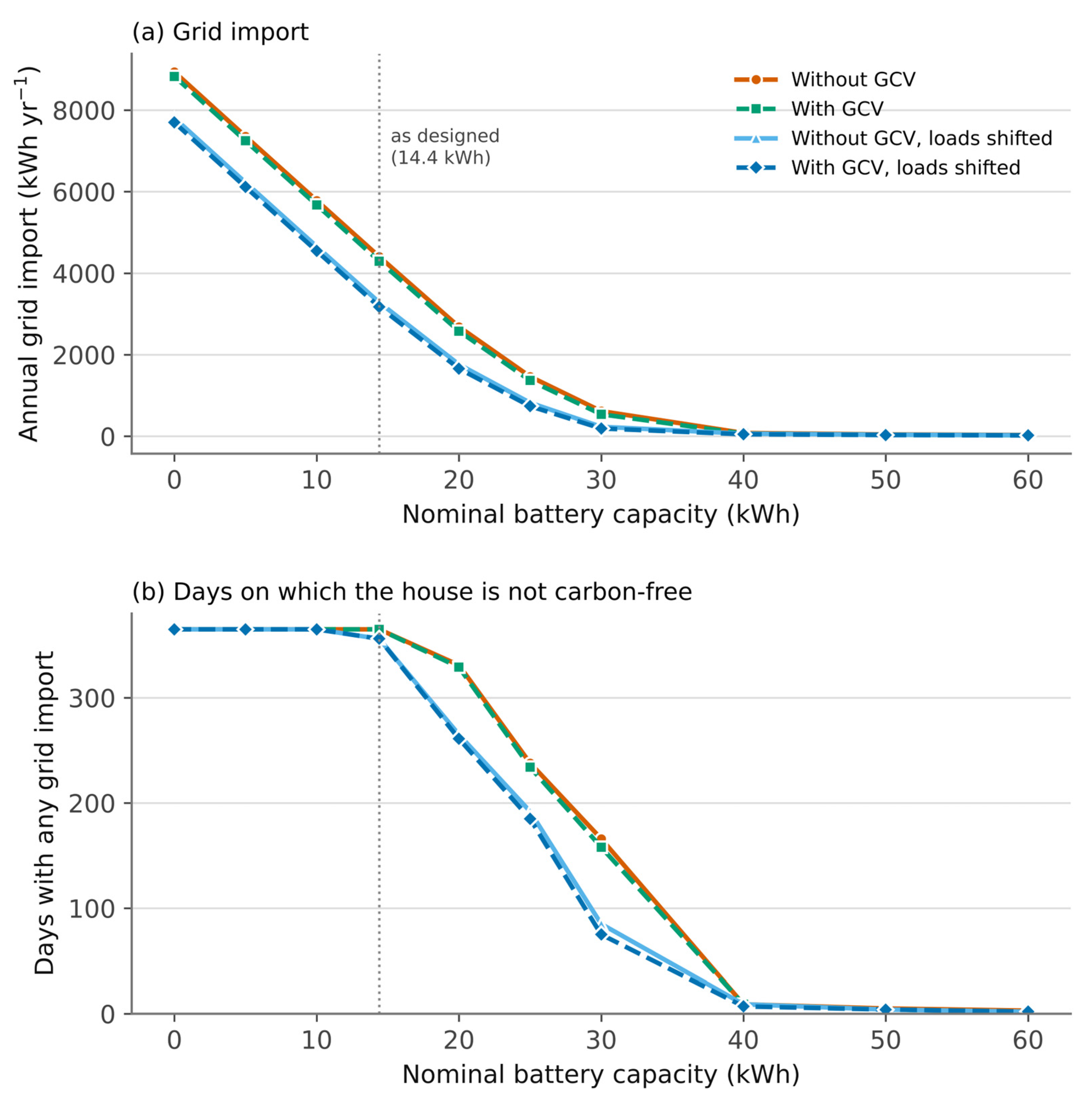
Figure 9 tests the claim that storage is the binding constraint. With an AC-coupled lithium-ion battery that can be charged from any surplus, the 14.4 kWh capacity of the design would already reduce imports to 4405 kWh y−1. Imports fall steeply with capacity, to 618 kWh y−1 at 30 kWh and 82 kWh y−1 at 40 kWh, at which point the house is carbon-free on all but 9 days of the year. Demand shifting lowers the curve by about 1100 kWh y−1 at small capacities and, at 40 kWh, brings imports to 64 kWh y−1 on 9 days, or 50 kWh y−1 on 7 days with the ground loop as well. The ground loop moves each curve by no more than 110 kWh y−1. Beyond 40 kWh the remaining imports occur on the few days of low solar output identified above, and would require storage over several days rather than within the day [47].
Figure 9.
Effect of battery capacity (AC-coupled lithium-ion, 92% round trip) on (a) annual grid import and (b) the number of days with any grid import, with and without the GCV system and demand shifting. Dashed lines denote the cases with the GCV system; the vertical dotted line marks the 14.4 kWh capacity of the design.
3.6. Operational Carbon
Table 10 converts the energy results into carbon at the central grid emission factor of 0.65 kgCO2 kWh−1. On the demand-side convention, the carbon associated with household electricity falls from 11.93 to 11.75 tCO2 y−1 with the ground loop, a saving of 0.18 tCO2 y−1 net of fan energy (0.15–0.20 t across the emission-factor band of 0.55 to 0.75 kgCO2 kWh−1), and carbon intensity falls from 147 to 145 kgCO2 m−2 y−1. On the net convention, in which the net exchange with the grid is valued, the house avoids 6.09 tCO2 y−1 without and 6.26 tCO2 y−1 with the ground loop. Valued only on the electricity actually purchased, grid-import carbon is 3.22 tCO2 y−1; it falls by 0.07 tCO2 y−1 with the ground loop, by 0.73 tCO2 y−1 with demand shifting, and to 0.03 tCO2 y−1 with demand shifting, the ground loop and a 40 kWh battery.
Table 10.
Annual operational carbon at a grid emission factor of 0.65 kgCO2 kWh−1.
Set against the household’s own consumption, the ground loop removes about 1.5% of the operational carbon of its electricity. Storage and demand scheduling act on the hours that are actually supplied from the fossil-fueled grid, and that is where the carbon is.
3.7. Economic Assessment
The capital cost of the single-pipe system, priced with the unit rates of the original quotation, is 18,802 SAR (5014 USD; Table 11): 4082 SAR for 32.4 m of pipe including risers, 3720 SAR for about 124 m3 of excavation in a trench 0.8 m wide and 6.3 m deep, and 11,000 SAR for the fan package, ducting and installation. For reference, the ten-pipe loop sized in the thesis would require 210.6 m of pipe and, at 1.0 m spacing between pipes, about 1340 m3 of excavation, for a total of 77,770 SAR; at the 3 m spacing needed to avoid thermal interference in limestone [41], the excavation would rise to about 3720 m3 and the total to 149,212 SAR. The cost of 80,420 SAR reported in the thesis [29] was for an earlier pipe configuration (170 m of 0.61 m pipe and 1600 m3 of excavation) and is superseded by these estimates.
Table 11.
Capital and operating cost of the ground-coupled ventilation system (Saudi market unit prices).
For the case-study house, the value of the saving depends on what the saved electricity otherwise would have cost. Of the 270 kWh y−1 removed from demand, 111 kWh y−1 reduces purchases from the grid; the remaining 158 kWh y−1 is exported at 0.07 SAR kWh−1. The ground loop is therefore worth 31 SAR y−1 (8.3 USD y−1), against 500 SAR y−1 of maintenance, and its net present value is negative at every discount rate examined, between −25,973 and −31,844 SAR (Table 12). Even with no maintenance cost at all, the net present value is about −21,000 SAR. With maintenance, the levelized cost of the electricity saved is 7.1 SAR kWh−1 (1.9 USD kWh−1) at a 5% discount rate, about forty times the tariff. No payback exists. Valuing every saved kilowatt-hour at the full tariff, as for the same house without photovoltaics, would raise the benefit only to 49 SAR y−1.
Table 12.
Life-cycle economic indicators of the single-pipe GCV system for the case-study house (capital 18,802 SAR; maintenance 500 SAR y−1; fan replaced after 15 years; 30-year analysis period).
The ten-pipe loop would make sense only in a building that must take in about 435 L s−1 of outdoor air. Even there, with the saving measured against a baseline carrying the same air, its levelized cost of saved electricity would be 0.94 SAR kWh−1 at 1 m pipe spacing and 1.70 SAR kWh−1 at 3 m, three to nine times the residential tariffs of 0.18–0.30 SAR kWh−1. At the prevailing tariffs, ground-coupled ventilation is not an economic measure for Saudi dwellings, whatever its sizing; it would need either a capital subsidy or a price signal that reflects the cost of supplying the summer peak.
4. Discussion
4.1. What Ventilation-Side Pre-Cooling Can and Cannot Do
The central result is that ground-coupled ventilation is thermally effective in Riyadh but has little to work on in a house of this kind. The pipe cools the outdoor air by 4.8 K on average and by up to 12.6 K, over ground that remains within 23–28 °C at 6 m depth throughout the year (Figure 3), and the pre-cooling is entirely sensible. However, the outdoor air of a two-person dwelling ventilated at the code rate, or ventilated more generously through an energy-recovery exchanger as this house is, carries only a few per cent of the cooling load of a house with walls of 5.36 m2 K W−1 thermal resistance, triple glazing, external shading and a vegetated west wall. Most of that load enters through the glazing and arises from internal gains, and a ventilation-side measure cannot reach it.
The result is bounded in two further directions. Seasonally, the loop contributes little in winter; the space heating it can displace, 920 kWh y−1 in the HAP model and most of it at night, can be reduced only in the hours in which the house needs heating and no cooling, and pre-heating adds 68 kWh y−1 to the saving. Structurally, cooling-load reduction was not the constraint that prevented carbon-free operation. The house imports electricity every night because the array produces in the middle of the day and the battery, charged from a 12-module sub-array through a 2.5 kW charger, cannot carry the evening and the night (Figure 8). Shifting deferrable appliance use into the solar window was about ten times as effective as the ground loop in reducing purchases, and a battery of about 40 kWh, roughly three times the designed capacity, combined with that shift would make the house carbon-free on all but seven to nine days of the year (Figure 9). Battery storage is well suited to this daily mismatch but not to multi-day deficits [47], and its value relative to demand response depends strongly on the tariff and export arrangements [48]. This reframes the design problem for solar houses in hot arid climates; once the envelope is good, further load reduction mostly buys export at 0.07 SAR kWh−1, while autonomy is bought with storage and scheduling.
4.2. Comparison with the Literature
Table 13 compares the present results with EAHE studies in hot arid and semi-arid climates. The temperature drops are of the same order; the mean drop of 4.8 K and maximum of 12.6 K over a 19.8 m pipe compare with maximum drops of about 19 K across the much longer pipes, or higher velocities, of studies in Morocco and Algeria [16,17]. Where the benefit is expressed per installation or per building rather than per unit of air, the figures fall to the magnitude found here—about 250 kWh y−1 for a single EAHE in southern Algeria [22], a net saving of only 25 kWh after fan energy over a monitoring campaign in Biskra, where bypass and fan shut-off under weak gradients proved important [20], and a 1.25–3.97% reduction in annual cooling load in Kerman [21]. Larger whole-building effects in the literature come from systems that move large volumes of outdoor air, typically into conventional or free-running dwellings [49,50], which is the situation reproduced by the 435 L s−1 case of Table 8. The comparison with refrigerant-based geothermal systems is also instructive. Ground-source heat pumps condition the whole load: reductions in electricity use of 40–50% have been reported for Saudi case studies [26], and of 47% for a heat pump combined with photovoltaic-thermal collectors in an arid residential building [27], although such systems have been found technically superior but economically marginal in hot dry climates [25]. The open-loop ventilation system avoids the compressor but, at the airflow a dwelling needs, addresses too small a share of the load to matter.
Table 13.
Reported performance of earth–air heat exchangers in hot arid and semi-arid climates compared with the present study.
One methodological point deserves comment, because it will occur to any reader of a carbon study. The house imports electricity at night and exports it at midday, and in a grid with substantial variable renewable capacity those two hours would carry very different carbon intensities, so that a single annual emission factor would misstate the result. In the Saudi system as it stands, the objection has little force: with 98% of generation fossil-fueled and solar and wind together at 2% [37], the diurnal variation in grid carbon intensity is small, and a single annual factor is an adequate approximation. That will not remain true. As the National Renewable Energy Programme adds capacity, midday grid intensity will fall faster than night-time intensity, the credit earned by exported solar generation will shrink and the penalty attached to night-time import will grow. The economic case for storage and for demand scheduling identified in Section 4.1 is therefore also, prospectively, a carbon case, and future studies of this kind in the Kingdom should move to time-resolved emission factors as soon as the data support it.
4.3. Practical Considerations
Open-loop ground pipes raise questions of air quality that any installation should address. Condensation in the pipe, and the biological growth it can support, is the main concern in temperate and humid climates [51], and fungal growth inside an earth tube has been measured in summer even where the supply air was not affected [52]. In Riyadh the risk of condensation in the cooling season is low: at the design condition the outdoor air holds about 3.0 g kg−1 of moisture, a dew point of about −4 °C, far below the pipe temperature of 23–28 °C. Dust is the greater practical issue. The design therefore includes a hooded intake with a sand screen and a coarse filter, whose pressure drop dominates the fan power (Section 3.4); the pipe should be laid to a fall towards a drained, accessible clean-out at its low point; and the glazed bore of vitrified clay allows camera inspection and cleaning. Inspection and filter replacement are covered by the maintenance allowance of Section 2.7.
A further option is to use surplus photovoltaic electricity for domestic hot water through an air-source heat pump water heater. The case-study house produces its hot water with evacuated-tube solar collectors [34], so the water heating demand itself is already met by solar heat; however, a heat pump water heater operated in the solar window would act as a low-cost thermal store for surplus electricity, and with appropriate control has been shown to reduce the purchased electricity for water heating by close to 90% [53]. Its cold exhaust air could also be ducted to pre-cool the ventilation air, a role that overlaps with that of the ground loop at a fraction of its cost. The option is not simulated here because the hot-water draw profile of the house is not available at hourly resolution, but it is a natural complement to the demand-shifting measures of Section 3.5.
4.4. Limitations
The main limitations of the study are as follows:
- •
- The study is a simulation exercise. No ground-coupled system was built and no metered energy data from the house in use were available, so the baseline could not be calibrated against measured consumption [46], as recent Saudi studies have done with utility bills [4]. The validation is model-to-model, and the GCV tool was validated by its author against the monitored system of the Solar CM House at Virginia Tech and against computational fluid dynamics, but not against a Riyadh installation of this configuration;
- •
- The typical meteorological year represents past climate. Riyadh summers are projected to warm by 2.1–4.1 °C by 2061–2080 under RCP4.5 [54], which would increase the cooling load and the temperature difference available to the ground loop, but not the share of the load carried by the outdoor air;
- •
- The house was deliberately left otherwise unchanged in the main analysis. Appliance schedules, battery capacity, array size and envelope were held at their design values so that the effect of the ground loop could be isolated. The storage and demand-shifting scenarios of Section 3.5 are indicative rather than optimized designs;
- •
- The battery model is a state-of-charge model with a fixed round-trip efficiency, power limits and a state-of-charge window. It does not represent ageing, the effect of temperature on capacity, or the control logic of the actual charger beyond its documented 2.5 kW limit, and the 12-module sub-array was assumed to produce one quarter of the output of the main array;
- •
- The conversion of delivered cooling to electricity uses the hourly coefficient of performance implied by the HAP model of the cooling plant. A different plant, or part-load behavior not captured by HAP, would change the proportion of electrical saving;
- •
- The effectiveness of the total-energy exchanger was inferred from the ventilation loads of the HAP design report, and the outdoor air reaching the coil from those loads and the hourly results, rather than read from the model file of the re-modeled house. The ventilation-rate sensitivity and the as-designed case of Table 8 bracket the consequence;
- •
- Space heating in the house is electric, and it was taken as HAP models it, with an input equal to the load. About half of it (485 kWh y−1) falls in hours in which the variable-air-volume model also cools the supply air, a reheat pattern that a single-zone unit would not reproduce, so the heating electricity, and with it the heating part of the ground-loop saving, may be overstated. This does not affect any conclusion;
- •
- The case-study building is not representative of the Saudi housing stock. It was designed to win a competition scored on energy performance, not to be economically viable, and its envelope is far better than that of a typical villa;
- •
- The design documentation was produced by several student and academic teams over a short period and contains internal inconsistencies, so some input values carry more uncertainty than the precision of the reported figures implies;
- •
- The fan power was calculated from assumed component pressure drops and an assumed fan–motor efficiency. Doubling the total pressure drop would double the fan energy to about 90 kWh y−1 and reduce the net saving to 225 kWh y−1, which does not affect any conclusion;
- •
- Costs are estimates from unit prices quoted for an earlier configuration at a single point in time. The pipe price is an upper bound for the smaller diameter, and the excavation price is the upper bound for limestone, the most expensive ground to excavate in the Kingdom. Halving the capital cost would leave the net present value negative, because the annual benefit is smaller than the maintenance cost;
- •
- Carbon is reported as operational carbon only, using a single annual grid emission factor. Embodied carbon in the pipework, the excavation and the photovoltaic array are excluded, as is any end-of-life accounting, so the figures in Section 3.6 are not life-cycle results and should not be read as such.
4.5. Implications and Directions for Further Work
Three directions follow directly from the results. The first is demand scheduling and storage; the scenarios of Section 3.5 show that shifting deferrable loads into the solar window and enlarging storage to about 40 kWh would bring the house close to carbon-free operation, and the next step is to test those measures with a calibrated model and with their own economics, including the effect of moving appliance heat gains into the peak cooling period and the thermal-storage option of a heat pump water heater. The second is the ground loop itself, which should be assessed in building types that must take in large volumes of outdoor air, such as assembly spaces, mosques, schools and clinics, where Table 8 suggests that a far larger share of the load is addressable, with soil saturation and pipe spacing modeled explicitly. The third is measurement: a monitored installation in Riyadh limestone would remove the main uncertainty in the design tool output and provide the data needed to calibrate both the tool and the building model.
5. Conclusions
This study assessed whether a ground-coupled ventilation system can bring an existing net-zero-energy solar house in Riyadh to carbon-free operation. The following conclusions are drawn:
- •
- At the outdoor-air rate required by ASHRAE 62.2 (20 L s−1), a single vitrified clay pipe 19.8 m long, 0.30 m in diameter and buried 6 m deep in limestone, cooled the ventilation air by 4.8 K on average over 4623 h, delivering 534 kWh y−1 of sensible cooling, and pre-heated it in winter, displacing 68 kWh y−1 of electric heating. This reduced HVAC electricity by 315 kWh y−1 (2.8%), or 270 kWh y−1 (2.4%) net of fan energy, and total household electricity by 1.5%.
- •
- The saving is small because the outdoor air is a small part of the cooling load of a well-insulated, lightly occupied house. It scales with the outdoor-air flow and would reach 32% only if 435 L s−1 of untreated outdoor air, the supply-air flow of the air-handling unit, were brought in, in which case the baseline itself would consume 89% more HVAC electricity. Where the outdoor air already passes through an energy-recovery exchanger, as in the house as designed, the exchanger takes most of the temperature difference that the loop would use, and the net saving is 3.2%. Coupling a ground loop to the supply-air flow rather than to the outdoor-air requirement overstates its benefit;
- •
- Bypass control is essential. Without it, the loop would warm the ventilation air in the 3757 h in which the house still needs cooling, cancelling most of the saving;
- •
- Strict carbon-free operation was not achieved. With the 14.4 kWh battery as designed the house imported 4961 kWh y−1, almost all of it at night and on every day of the year. The ground loop reduced imports by 2.2% and shifted 3.1 kWh d−1 of evening appliance use to midday by 23%, while a 40 kWh battery combined with that shift reduced them to 50–64 kWh y−1 on seven to nine days;
- •
- At a grid emission factor of 0.65 kgCO2 kWh−1 the ground loop avoids 0.18 tCO2 y−1, about 1.5% of the operational carbon of the household’s electricity;
- •
- The ground loop is not economically viable for this house at the prevailing tariffs. Its energy benefit of about 31 SAR y−1 is smaller than its maintenance cost, its net present value is negative at discount rates of 3–8%, and its levelized cost of saved electricity exceeds the tariff by a factor of about forty. Even a loop sized for 435 L s−1 of outdoor air would cost 0.9–1.7 SAR per kilowatt-hour saved.
The wider implication is that, once the envelope of a Saudi solar house is good, reaching carbon-free operation is a storage and demand-management problem rather than a cooling problem. Ground-coupled ventilation remains a sound way to temper outdoor air in this climate, but it belongs in buildings that must take in large volumes of outdoor air, and even there it would need capital support or cost-reflective tariffs to be attractive to owners on economic grounds alone.
Supplementary Materials
The following supporting information can be downloaded at: https://www.mdpi.com/article/10.3390/en19215355/s1. Table S1: Hourly energy balance of the case-study house (8760 h) for the baseline, GCV, battery and demand-shifting cases; File S1: Analysis script reproducing the results of Section 2.4, Section 2.5, Section 2.6, Section 2.7, Section 2.8, Section 3, Section 3.1, Section 3.2, Section 3.3, Section 3.4, Section 3.5, Section 3.6 and Section 3.7; File S2: Raw-data package (original design documentation, HAP files and GCV tool output).
Author Contributions
Conceptualization, O.A. and M.G.K.; methodology, O.A., M.G.K. and M.O.A.; software, O.A. and M.O.A.; validation, O.A. and M.O.A.; formal analysis, O.A. and A.G.K.; investigation, O.A.; data curation, O.A.; writing—original draft preparation, O.A.; writing—review and editing, M.G.K., M.O.A. and A.G.K.; visualization, A.G.K.; supervision, M.G.K.; project administration, A.G.K. All authors have read and agreed to the published version of the manuscript.
Funding
This research was funded by the Ongoing Research Funding Program (ORF-2026-xxxx), King Saud University, Riyadh, Saudi Arabia.
Data Availability Statement
The hourly energy-balance data and the analysis script supporting the reported results are provided as Supplementary Materials. The original design documentation, the HAP load-calculation files and the GCV tool output are included in the supplementary raw-data package; the HelioScope project and the HAP model of the re-modeled house are available from the authors on request.
Acknowledgments
The authors thank the Team KSU Solar Decathlon Middle East group 2018 at King Saud University for access to the project documentation for the case-study house. During the preparation of this manuscript, the authors used Claude (Anthropic, Opus model series, accessed September–October 2026) for drafting text from the first author’s thesis, writing and running the scripts that recompute the hourly coupling, fan, battery, operational carbon and economic results from the hourly simulation output, drawing Figure 1, Figure 3, Figure 4, Figure 5, Figure 6, Figure 7, Figure 8 and Figure 9 and the legend of Figure 2, and searching for and checking references. The authors have reviewed and edited the output and take full responsibility for the content of this publication.
Conflicts of Interest
The authors declare no conflicts of interest.
Abbreviations
The following abbreviations are used in this manuscript:
| ACH | Air changes per hour |
| AHU | Air-handling unit |
| CO2 | Carbon dioxide |
| COP | Coefficient of performance |
| CRF | Capital recovery factor |
| EAHE | Earth–air heat exchanger |
| EUI | Energy use intensity |
| GCV | Ground-coupled ventilation |
| HAP | Hourly Analysis Program (Carrier) |
| HVAC | Heating, ventilation and air conditioning |
| KSU | King Saud University |
| LCSE | Levelized cost of saved electricity |
| NPV | Net present value |
| NTU | Number of transfer units |
| PV | Photovoltaic |
| SAR | Saudi riyal |
| SDME | Solar Decathlon Middle East |
| TMY | Typical meteorological year |
| USD | US dollar |
References
- Aldubyan, M. Future of residential electricity demand in Saudi Arabia and the role of energy efficiency in 2060’s net zero pledge. Dev. Sustain. Econ. Financ. 2025, 8, 100086. [Google Scholar] [CrossRef] [Scilit]
- Rodrigues, L.; Cherian, B.A.; Tokbolat, S. Reducing Cooling Energy Demand in Saudi Arabian Residential Buildings Using Passive Design Approaches. Buildings 2025, 15, 1895. [Google Scholar] [CrossRef] [Scilit]
- Alyami, M. The Impact of the Composition and Location of Thermal Insulation in the Building Envelope on Energy Consumption in Low-Rise Residential Buildings in Hot Climate Regions. Arab. J. Sci. Eng. 2024, 49, 5305–5351. [Google Scholar] [CrossRef] [Scilit]
- Aloshan, M.A. Achieving near-zero energy in hot climates: Retrofitting building envelopes for existing homes. Heliyon 2025, 11, e42170. [Google Scholar] [CrossRef] [Scilit]
- Abd-ur-Rehman, H.M.; Al-Sulaiman, F.A.; Mehmood, A.; Shakir, S.; Umer, M. The potential of energy savings and the prospects of cleaner energy production by solar energy integration in the residential buildings of Saudi Arabia. J. Clean. Prod. 2018, 183, 1122–1130. [Google Scholar] [CrossRef] [Scilit]
- Elshurafa, A.M.; Alatawi, H.; Al-Saikhan, A.; Al-Hsaien, S.A. Solar PV on mosque rooftops: Results from a pilot study in Saudi Arabia. J. Build. Eng. 2019, 25, 100809. [Google Scholar] [CrossRef] [Scilit]
- Imam, A.A.; Al-Turki, Y.A.; Sreerama Kumar, R. Techno-Economic Feasibility Assessment of Grid-Connected PV Systems for Residential Buildings in Saudi Arabia—A Case Study. Sustainability 2020, 12, 262. [Google Scholar] [CrossRef] [Scilit]
- Al-Hanoot, A.K.; Mokhlis, H.; Mekhilef, S.; Alghoul, M.; Shareef, H.; Samatar, A.M. Distributed PV systems in Saudi Arabia: Current status, challenges, and prospects. Energy Strategy Rev. 2024, 55, 101535. [Google Scholar] [CrossRef] [Scilit]
- Shirinbakhsh, M.; Harvey, L.D.D. Net-zero energy buildings: The influence of definition on greenhouse gas emissions. Energy Build. 2021, 247, 111118. [Google Scholar] [CrossRef] [Scilit]
- Wang, D.; Lin, Y. A comprehensive review on definitions, development, and policies of net-zero carbon buildings (nZCBs). Renew. Sustain. Energy Rev. 2025, 217, 115750. [Google Scholar] [CrossRef] [Scilit]
- Imanloozadeh, A.; Lubitz, W.D. Characteristics, design, and optimization of earth-air heat exchangers: A review. Renew. Sustain. Energy Rev. 2026, 230, 116677. [Google Scholar] [CrossRef] [Scilit]
- Koshlak, H. A review of earth-air heat exchangers: From fundamental principles to hybrid systems with renewable energy integration. Energies 2025, 18, 1017. [Google Scholar] [CrossRef] [Scilit]
- Zhao, J.; Huang, B.; Li, Y.; Zhao, Y. Comprehensive review on climatic feasibility and economic benefits of Earth-to-Air Heat Exchanger (EAHE) systems. Sustain. Energy Technol. Assess. 2024, 68, 103862. [Google Scholar] [CrossRef] [Scilit]
- Soares, N.; Rosa, N.; Monteiro, H.; Costa, J.J. Advances in standalone and hybrid earth-air heat exchanger (EAHE) systems for buildings: A review. Energy Build. 2021, 253, 111532. [Google Scholar] [CrossRef] [Scilit]
- Mihalakakou, G.; Souliotis, M.; Papadaki, M.; Halkos, G.; Paravantis, J.; Makridis, S.; Papaefthimiou, S. Applications of earth-to-air heat exchangers: A holistic review. Renew. Sustain. Energy Rev. 2022, 155, 111921. [Google Scholar] [CrossRef] [Scilit]
- Khabbaz, M.; Benhamou, B.; Limam, K.; Hollmuller, P.; Hamdi, H.; Bennouna, A. Experimental and numerical study of an earth-to-air heat exchanger for air cooling in a residential building in hot semi-arid climate. Energy Build. 2016, 125, 109–121. [Google Scholar] [CrossRef] [Scilit]
- Belloufi, Y.; Zerouali, S.; Rouag, A.; Aissaoui, F.; Atmani, R.; Brima, A.; Moummi, N. Transient assessment of an earth air heat exchanger in warm climatic conditions. Geothermics 2022, 104, 102442. [Google Scholar] [CrossRef] [Scilit]
- Serageldin, A.A.; Abdelrahman, A.K.; Ookawara, S. Earth-Air Heat Exchanger thermal performance in Egyptian conditions: Experimental results, mathematical model, and Computational Fluid Dynamics simulation. Energy Convers. Manag. 2016, 122, 25–38. [Google Scholar] [CrossRef] [Scilit]
- Agrawal, K.K.; Misra, R.; Yadav, T.; Agrawal, G.D.; Jamuwa, D.K. Experimental study to investigate the effect of water impregnation on thermal performance of earth air tunnel heat exchanger for summer cooling in hot and arid climate. Renew. Energy 2018, 120, 255–265. [Google Scholar] [CrossRef] [Scilit]
- Ounis, S.; Boucherit, O.; Moummi, A.; Bouzir, T.A.K.; Berkouk, D.; Leonforte, F.; Del Pero, C.; Gomaa, M.M. A hybrid earth–air heat exchanger with a subsurface water tank: Experimental validation in a hot–arid climate. Sustainability 2025, 17, 10216. [Google Scholar] [CrossRef] [Scilit]
- Mostafaeipour, A.; Goudarzi, H.; Khanmohammadi, M.; Jahangiri, M.; Sedaghat, A.; Norouzianpour, H.; Chowdhury, S.; Techato, K.; Issakhov, A.; Almutairi, K.; et al. Techno-economic analysis and energy performance of a geothermal earth-to-air heat exchanger (EAHE) system in residential buildings: A case study. Energy Sci. Eng. 2021, 9, 1807–1825. [Google Scholar] [CrossRef] [Scilit]
- Belatrache, D.; Bentouba, S.; Bourouis, M. Numerical analysis of earth air heat exchangers at operating conditions in arid climates. Int. J. Hydrogen Energy 2017, 42, 8898–8904. [Google Scholar] [CrossRef] [Scilit]
- Alaidroos, A.; Krarti, M. Evaluation of Passive Cooling Systems for Residential Buildings in the Kingdom of Saudi Arabia. J. Sol. Energy Eng. 2016, 138, 031011. [Google Scholar] [CrossRef] [Scilit]
- Ouzzane, M.; Naqash, M.T.; Harireche, O. Assessment of the Potential Use of Shallow Geothermal Energy Source for Air Heating and Cooling in the Kingdom of Saudi Arabia. Nat. Environ. Pollut. Technol. 2021, 20, 1923–1934. [Google Scholar] [CrossRef] [Scilit]
- Alshehri, F.; Beck, S.; Ingham, D.; Ma, L.; Pourkashanian, M. Techno-economic analysis of ground and air source heat pumps in hot dry climates. J. Build. Eng. 2019, 26, 100825. [Google Scholar] [CrossRef] [Scilit]
- Aldubyan, M.; Al Suwailem, M.A.; Alali, A.; Alhani, A. Techno-Economic Evaluation of Shallow Geothermal Cooling in Saudi Arabia; Discussion Paper; King Abdullah Petroleum Studies and Research Center (KAPSARC): Riyadh, Saudi Arabia, 2026. [Google Scholar] [CrossRef] [Scilit]
- Ismaeil, E.M.H.; Sobaih, A.E.E. Heuristic approach for net-zero energy residential buildings in arid region using dual renewable energy sources. Buildings 2023, 13, 796. [Google Scholar] [CrossRef] [Scilit]
- ANSI/ASHRAE 62.2-2022; Ventilation and Acceptable Indoor Air Quality in Residential Buildings. American Society of Heating, Refrigerating and Air-Conditioning Engineers (ASHRAE): Atlanta, GA, USA, 2022.
- Alanazi, O.S. Ground Source Ventilation and Solar PV towards Zero Carbon Houses in Riyadh. Master’s Thesis, King Saud University, Riyadh, Saudi Arabia, 2022. [Google Scholar]
- ASHRAE. 2001 ASHRAE Handbook—Fundamentals; Chapter 29; American Society of Heating, Refrigerating and Air-Conditioning Engineers: Atlanta, GA, USA, 2001. [Google Scholar]
- Autodesk. Revit—Building Information Modelling Software; Autodesk Inc.: San Francisco, CA, USA; Available online: https://www.autodesk.com/revit (accessed on 20 October 2026).
- Carrier. Hourly Analysis Program (HAP); Carrier Global Corporation: Palm Beach Gardens, FL, USA; Available online: https://www.carrier.com/us/en/commercial/software/hvac-system-design/hourly-analysis-program/ (accessed on 20 October 2026).
- Aurora Solar. HelioScope—Commercial Solar Design Software; Aurora Solar Inc.: San Francisco, CA, USA; Available online: https://helioscope.aurorasolar.com/ (accessed on 20 October 2026).
- Team KSU. Solar Decathlon Middle East 2018—Project Manual and Design Documentation; King Saud University: Riyadh, Saudi Arabia, 2018. [Google Scholar]
- The MathWorks Inc. MATLAB; The MathWorks Inc.: Natick, MA, USA, 2018; Available online: https://www.mathworks.com/products/matlab.html (accessed on 20 October 2026).
- Alfadil, M.O. Design Tool for a Ground-Coupled Ventilation System. Ph.D. Thesis, Virginia Polytechnic Institute and State University, Blacksburg, VA, USA, 2021. Available online: http://hdl.handle.net/10919/100604 (accessed on 14 May 2021).
- Ember. Saudi Arabia: Electricity Profile; Yearly Electricity Data. Available online: https://ember-energy.org/countries-and-regions/saudi-arabia/ (accessed on 25 January 2024).
- Wajid, H.A. Saudi Arabia’s green leap: Unlocking the climate potential of the Haramain High-Speed Railway through occupancy optimization and renewable energy adoption. Front. Sustain. Cities 2025, 7, 1643872. [Google Scholar] [CrossRef] [Scilit]
- Kusuda, T.; Achenbach, P.R. Earth Temperature and Thermal Diffusivity at Selected Stations in the United States; NBS Report 8972; National Bureau of Standards: Washington, DC, USA, 1965. [Google Scholar] [CrossRef] [Scilit]
- Misra, R.; Bansal, V.; Agrawal, G.D.; Mathur, J.; Aseri, T.K. CFD analysis based parametric study of derating factor for Earth Air Tunnel Heat Exchanger. Appl. Energy 2013, 103, 266–277. [Google Scholar] [CrossRef] [Scilit]
- Minaei, A.; Rabani, R. Development of a transient analytical method for multi-pipe earth-to-air heat exchangers with parallel configuration. J. Build. Eng. 2023, 73, 106781. [Google Scholar] [CrossRef] [Scilit]
- Niu, F.; Yu, Y.; Yu, D.; Li, H. Investigation on soil thermal saturation and recovery of an earth to air heat exchanger under different operation strategies. Appl. Therm. Eng. 2015, 77, 90–100. [Google Scholar] [CrossRef] [Scilit]
- International Monetary Fund. Saudi Arabia: 2024 Article IV Consultation—Press Release and Staff Report; IMF Country Report No. 24/280; International Monetary Fund: Washington, DC, USA, 2024. [Google Scholar]
- Electricity and Cogeneration Regulatory Authority. Consumption Tariff Schedule for the Kingdom of Saudi Arabia; Approved by Council of Ministers’ Decree of 12 December 2017, Effective 1 January 2018; ECRA (now the Saudi Electricity Regulatory Authority): Riyadh, Saudi Arabia, 2018; Available online: https://rise.esmap.org/data/files/library/saudi-arabia/Renewable%20Energy/Saudi%20Arabia%20Tariff%20Schedule_2022.pdf (accessed on 20 October 2026).
- Electricity and Cogeneration Regulatory Authority. Regulatory Framework for Small-Scale Solar PV Systems; Document ERD-TA-012, Version 2; ECRA: Riyadh, Saudi Arabia, 2019; Available online: https://rise.esmap.org/sites/default/files/library/saudi-arabia/Renewable%20Energy/Kingdom%20of%20Saudi%20Arabia_Regulatory%20Framework%20for%20Small-%20Scale%20Solar%20PV%20Systems.pdf (accessed on 20 October 2026).
- ASHRAE. ASHRAE Guideline 14-2014: Measurement of Energy, Demand, and Water Savings; American Society of Heating, Refrigerating and Air-Conditioning Engineers: Atlanta, GA, USA, 2014. [Google Scholar]
- Rosati, A.; Facci, A.L.; Ubertini, S. Techno-economic analysis of battery electricity storage towards self-sufficient buildings. Energy Convers. Manag. 2022, 256, 115313. [Google Scholar] [CrossRef] [Scilit]
- Cai, Q.; Qing, J.; Xu, Q.; Shi, G.; Liang, Q.-M. Techno-economic impact of electricity price mechanism and demand response on residential rooftop photovoltaic integration. Renew. Sustain. Energy Rev. 2024, 189, 113964. [Google Scholar] [CrossRef] [Scilit]
- Al-Ajmi, F.; Loveday, D.; Hanby, V. The cooling potential of earth–air heat exchangers for domestic buildings in a desert climate. Build. Environ. 2006, 41, 235–244. [Google Scholar] [CrossRef] [Scilit]
- Benhammou, M.; Draoui, B.; Hamouda, M. Improvement of the summer cooling induced by an earth-to-air heat exchanger integrated in a residential building under hot and arid climate. Appl. Energy 2017, 208, 428–445. [Google Scholar] [CrossRef] [Scilit]
- Chardome, G.; Feldheim, V. Heat transfer and condensation in an earth-air heat exchanger: 2D/3D numerical modeling validated by experimental measurements. Energy Build. 2019, 205, 109532. [Google Scholar] [CrossRef] [Scilit]
- Kang, Y.; Nagano, K. Field measurement of indoor air quality and airborne microbes in a near-zero energy house with an earth tube in the cold region of Japan. Sci. Technol. Built Environ. 2016, 22, 1010–1023. [Google Scholar] [CrossRef] [Scilit]
- Clift, D.H.; Suehrcke, H. Control optimization of PV powered electric storage and heat pump water heaters. Sol. Energy 2021, 226, 489–500. [Google Scholar] [CrossRef] [Scilit]
- Kotbi, M.G.; Alsuhaibani, S.A.; Kotbi, A.G. Impact of Projected Climate Change on the Thermal Performance and Comfort of Residential Buildings in Riyadh, Saudi Arabia: Dynamic Simulation to 2070 and the Effectiveness of Envelope Improvement. Buildings 2026, 16, 3671. [Google Scholar] [CrossRef] [Scilit]
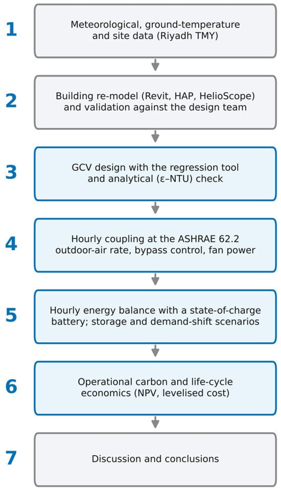
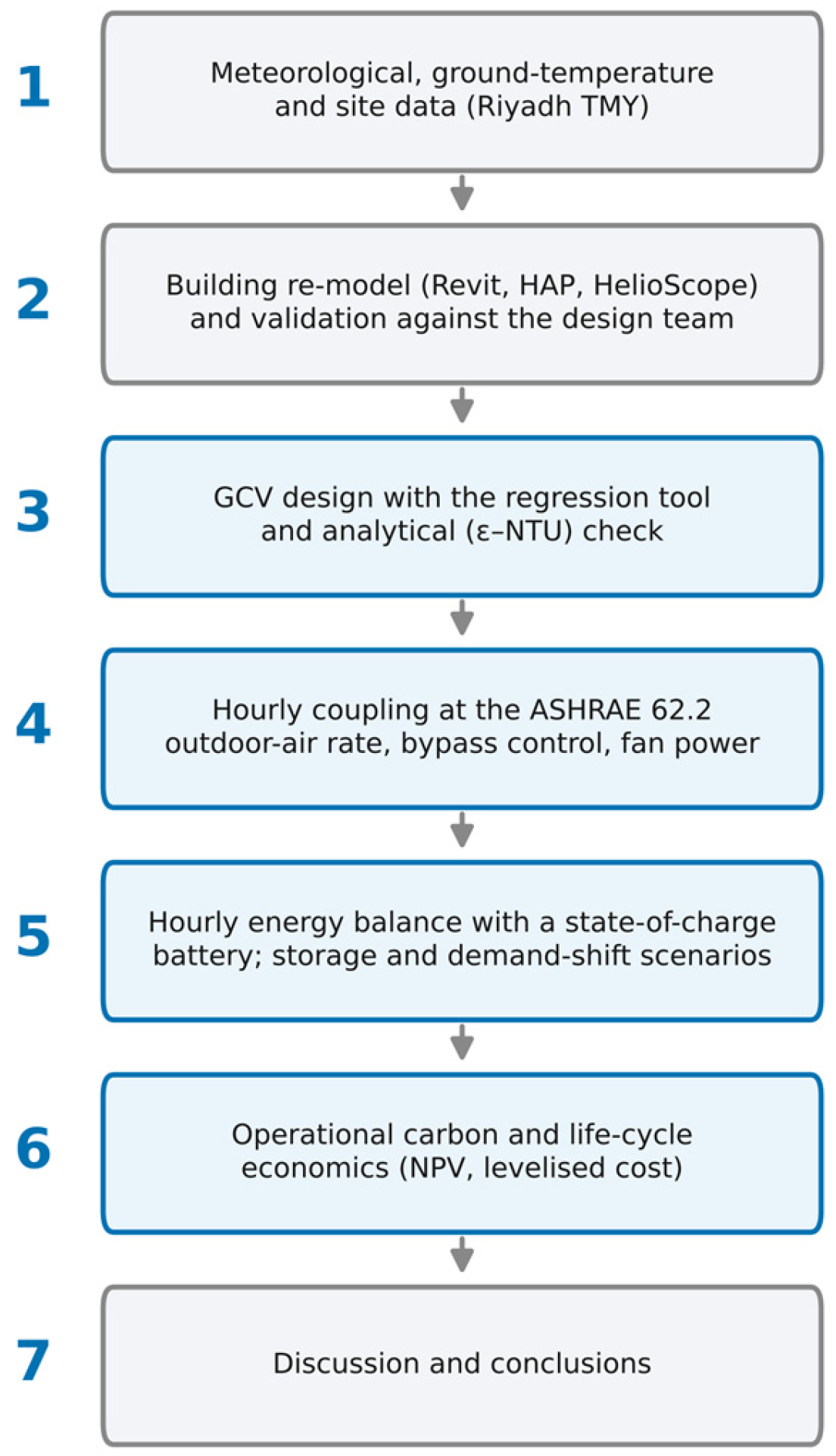
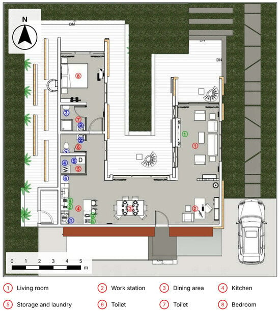
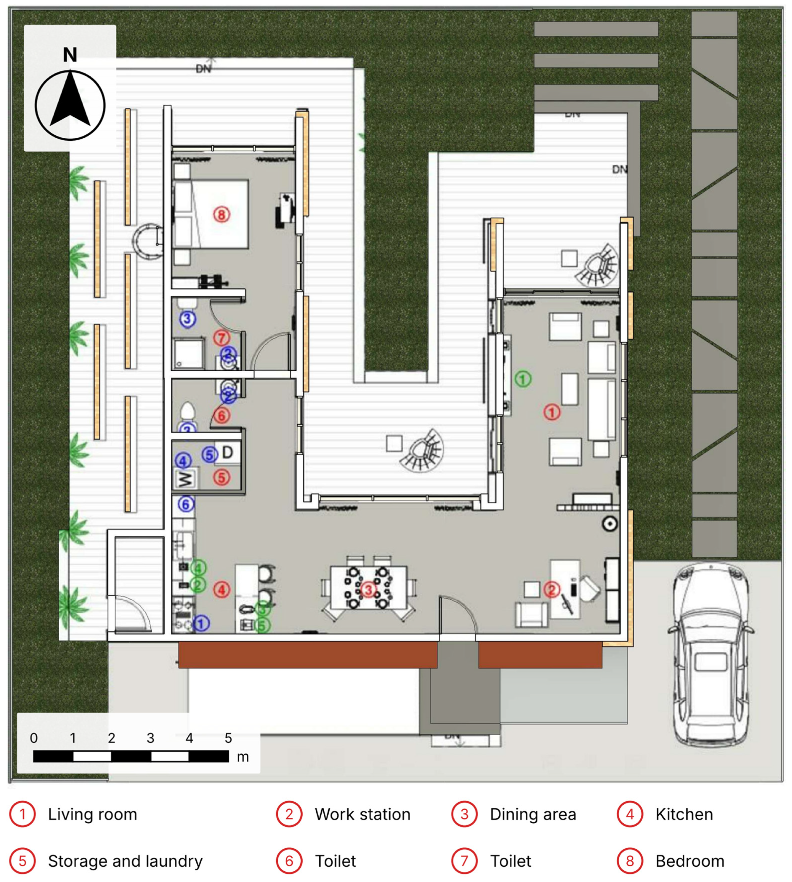
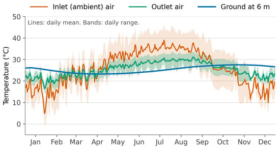
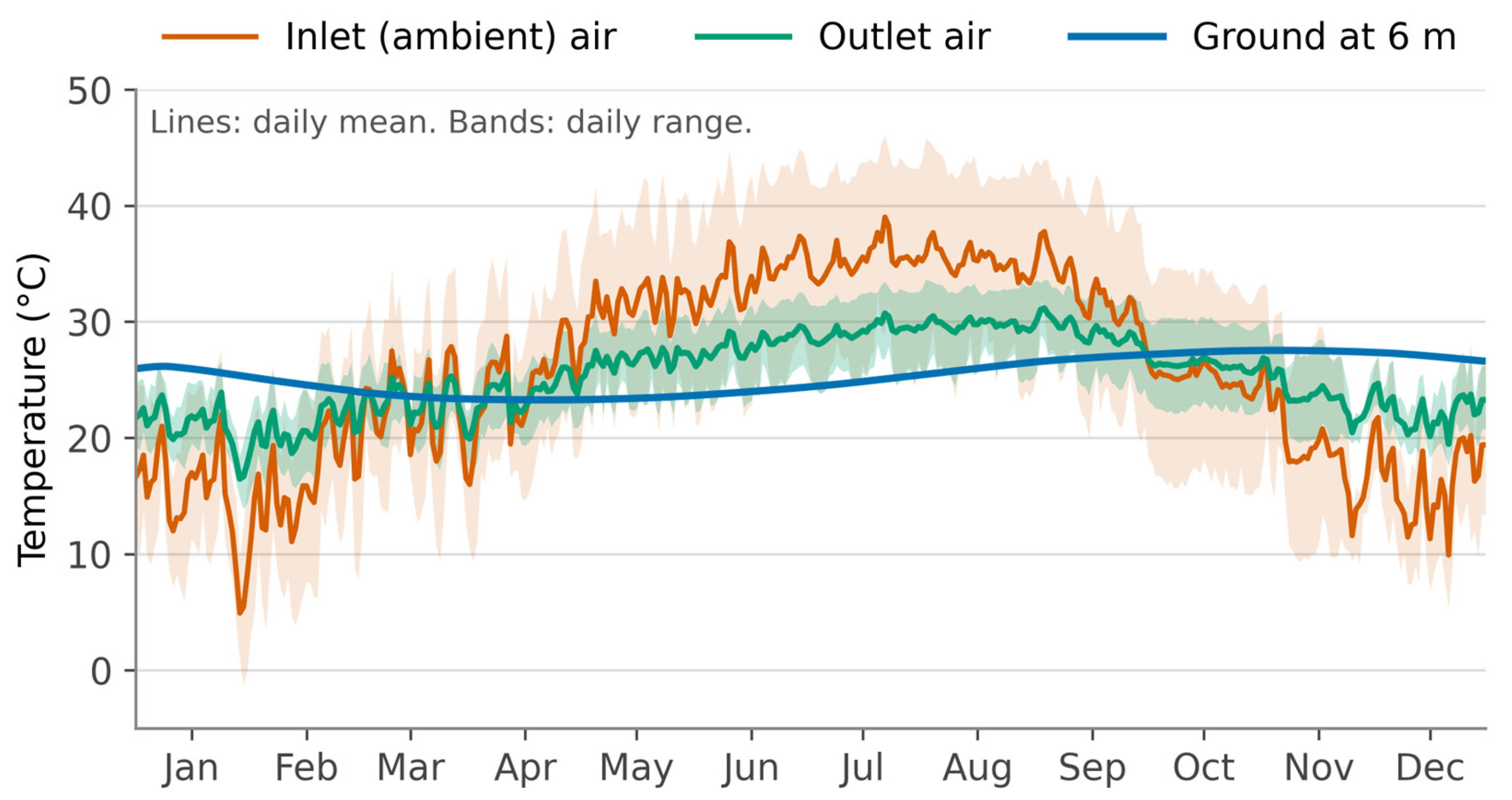

Disclaimer/Publisher’s Note: The statements, opinions and data contained in all publications are solely those of the individual author(s) and contributor(s) and not of MDPI and/or the editor(s). MDPI and/or the editor(s) disclaim responsibility for any injury to people or property resulting from any ideas, methods, instructions or products referred to in the content. |
© 2026 by the authors. Licensee MDPI, Basel, Switzerland. This article is an open access article distributed under the terms and conditions of the Creative Commons Attribution (CC BY) license.