


Abstract
Rapid electric vehicle adoption can create severe voltage, loading, and service-continuity constraints in low-voltage networks when demand growth is spatially uneven. This study evaluates a multi-terminal Smart Soft Open Point (SOP) framework for reinforcement deferral using a modified 47-bus CIGRE low-voltage benchmark and 8760-h nonlinear AC optimization. The principal case combines 1.5 times base demand with 200 electric vehicles and compares the existing benchmark network (BMK), Smart SOP, and conventional grid reinforcement (GRU). Smart SOP coordinates bidirectional active-power exchange, capacitive reactive support, and feeder-level served-load variables. It reduces annual energy not served from 15.36% to 3.72%, mean load-balancing index from 23.57% to 11.96%, and hours with more than 5% service reduction from 7059 to 2670. GRU nearly eliminates energy not served (0.04%) and provides the strongest voltage performance, but at substantially higher annual system cost. Capacity sensitivity shows diminishing returns beyond the baseline 402 kVA SOP rating, while Monte Carlo load uncertainty gives Smart SOP the highest median annual net value. The results indicate that Smart SOP can provide a lower-capital alternative to conventional reinforcement for concentrated electrification-driven growth while preserving substantially more service than the unreinforced network.
1. Introduction
Electrification of transport and other end uses is shifting final-energy demand toward electricity. Electric vehicles (EVs), heat pumps, electric cooking, and air conditioning can sharply increase coincident low-voltage (LV) feeder demand. Continued EV deployment therefore makes distribution capacity and hosting capability central planning concerns [1], particularly where thermal margins are limited and voltage drops are pronounced.
EV impacts depend on charger rating and location, arrival time, charging duration, and coincidence with background demand. Aggregated charging can produce concentrated peaks, while stochastic behavior changes transformer loading and feeder voltage [2,3]. Time-series assessment is therefore preferable to isolated snapshots [4]. Conventional transformer or conductor reinforcement provides direct headroom but can require large, irreversible investment and may be underutilized when growth is uncertain or spatially concentrated. Flexible interconnection can instead release spare capacity across neighboring feeders [5].
Soft open points (SOPs) replace or augment normally open mechanical ties with controllable power–electronic interfaces. Bidirectional active-power exchange and reactive support can provide feeder balancing, voltage regulation, and operational flexibility [6]. Steady-state SOP models commonly use controllable complex-power injections subject to active-power balance, converter losses, and apparent-power limits [7]. Planning studies have examined SOP siting and sizing [8], while reliability studies quantify the capacity value of redirecting available supply toward stressed feeders [9].
Multi-terminal SOPs extend controllable exchange across more than two feeders and can improve utilization of unequally loaded assets [10]. Three-phase formulations demonstrate operation under unbalanced conditions [11]. LV field-oriented work has shown that active transfer can balance feeder loading and reactive injection can support voltage, while highlighting the importance of location, losses, protection, and control strategy [12]. Hierarchical Volt/Var and Volt/Watt control provides a further route to coordinated voltage regulation [13].
Converter cost and utilization remain deployment barriers. Cost-effective converter arrangements [14] and cost–benefit studies [15] show that value depends on rating, utilization, losses, and the reinforcement alternative. EV-oriented studies have considered SOP expansion with traffic flow [16], coordinated SOP-charging operation [17], EV-SOP co-planning [18], mobile SOPs for charging-station hosting capacity [19], reactive-power-aware configuration [20], and three-port scheduling [21]. Vehicle-level studies further show that PHEV energy demand depends on driving behavior and supervisory energy management [22,23], while coordinated active- and reactive-power control has been investigated for voltage regulation [24].
A planning gap nevertheless remains between these specialized studies and the decision faced by an LV operator experiencing rapid load growth. Evidence is limited on full-year multi-terminal SOP operation when voltage quality, transformer utilization, service continuity, demand-side flexibility, converter sizing, losses, and annualized reinforcement economics are evaluated together. Improvements at selected operating points do not necessarily establish annual reliability or economic value.
Accordingly, this study treats Smart SOP as a system-level flexibility framework rather than a new converter topology. It combines a three-terminal SOP, bidirectional active-power exchange, capacitive reactive support, feeder-specific served-load variables, and measurement-enabled coordination. The framework is evaluated for 8760 hourly operating points on a modified 47-bus CIGRE LV benchmark. The principal case combines 1.5 times reference demand with 200 EVs and compares the existing benchmark network (BMK), Smart SOP, and conventional grid reinforcement (GRU). Additional load cases, SOP-capacity sensitivity, and Monte Carlo load variation test robustness.
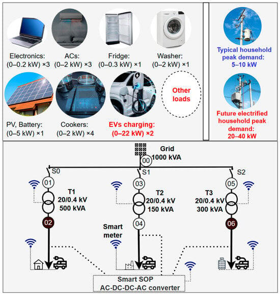
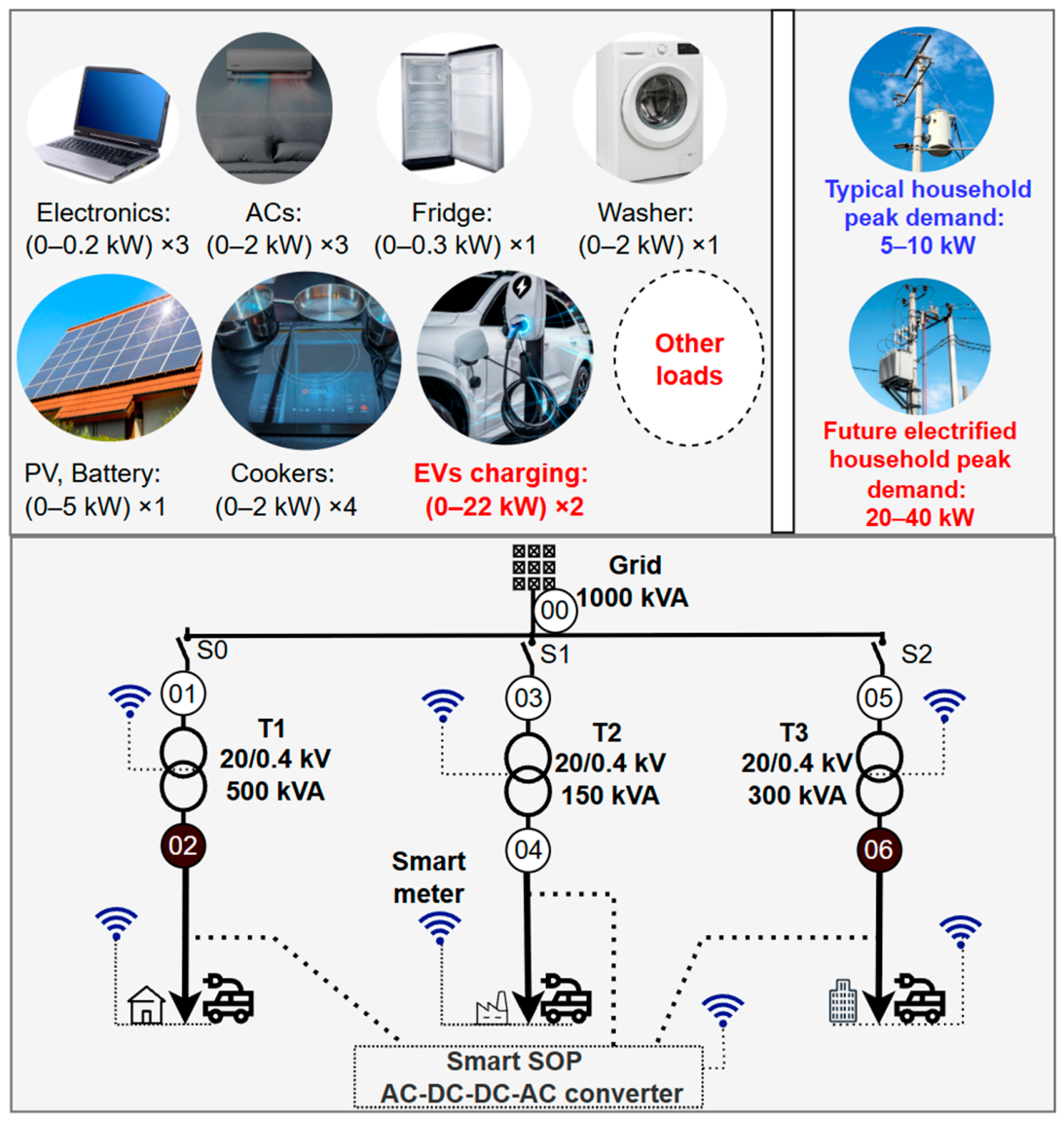
The contributions are: (1) full-year nonlinear AC optimization of an EV-loaded three-feeder LV network with voltage, transformer, converter-loss, and service-continuity constraints; (2) a common technical, reliability, and economic comparison of BMK, Smart SOP, and GRU; (3) feeder-specific served-load variables that quantify intervention frequency and severity; and (4) capacity-sensitivity and uncertainty analyses that expose diminishing returns and economic robustness. Figure 1 summarizes the planning problem and Smart SOP concept.
Figure 1.
Electrification-driven low-voltage network stress and the proposed three-terminal Smart SOP concept. Household power ranges are illustrative and are not simulation inputs.
2. System Description and Simulation Cases
2.1. Modified CIGRE Low-Voltage Network and Study Framework
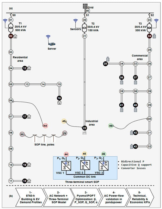
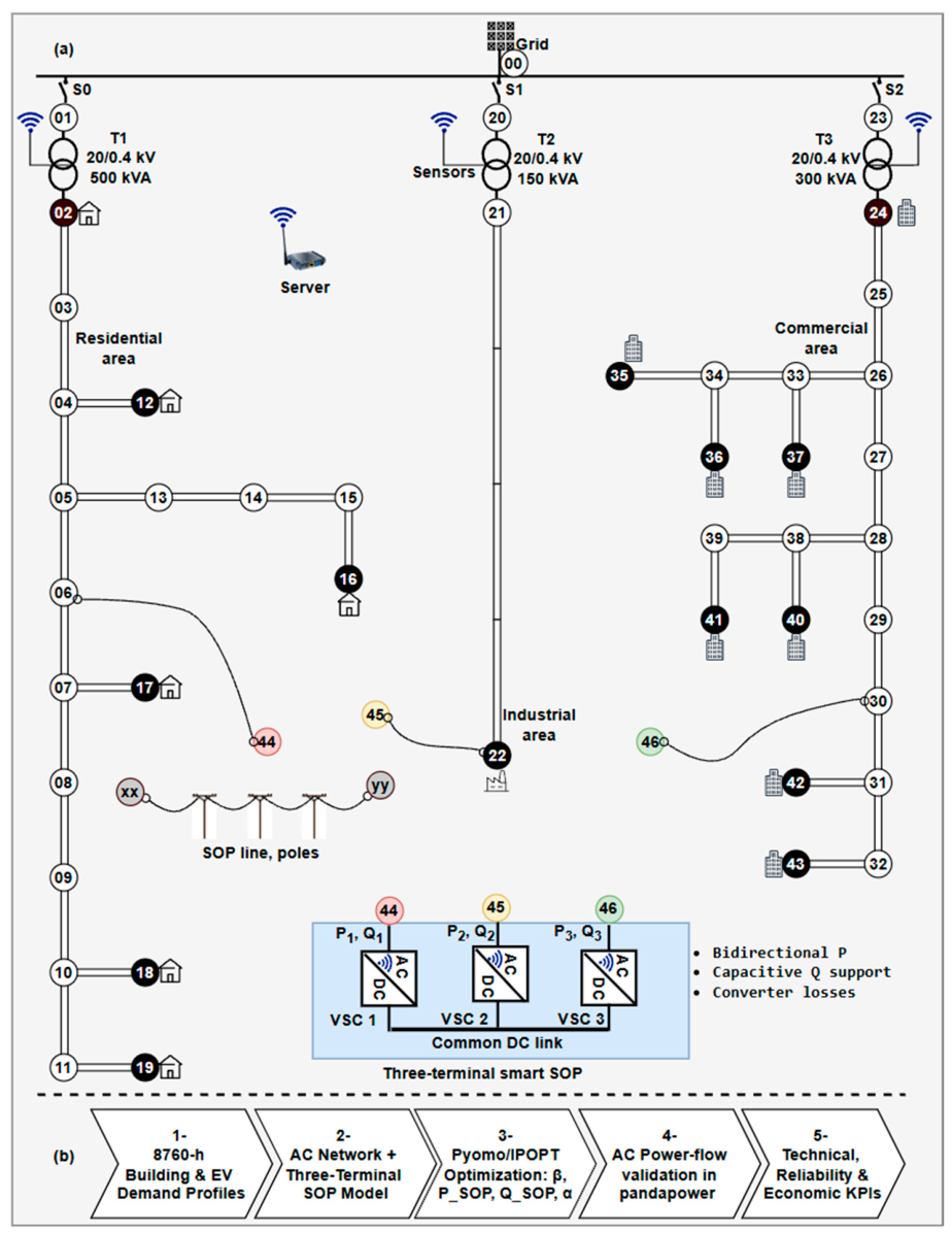
The study uses a modified 47-bus network derived from the European 400 V CIGRE LV benchmark supplied from a common 20 kV bus [25]. Smart SOP terminals are connected at buses 44, 45, and 46 near the remote ends of the residential, industrial, and commercial feeders. Transformers T1–T3 are rated at 500, 150, and 300 kVA, respectively, providing unequal capacity for testing controllable inter-feeder sharing. A 1 MVA base is used throughout. Customer allocation, hourly demand profiles, topology, and branch parameters are identical for BMK and Smart SOP. Bus 0 is the slack bus at 1.0 pu and 0 rad. The optimization enforces 0.85–1.10 pu voltage feasibility; exposure below 0.90 pu is reported separately.
The remote SOP locations permit active-power redistribution and local capacitive reactive support at electrically weak feeder sections [10]. For every network configuration, 8760-h building and EV profiles are assembled, network/SOP/service constraints are formulated in Pyomo [26], and hourly voltages, transformer injections, service factors, and SOP set points are optimized. Each operating point is then reconstructed independently in pandapower [27] before technical and economic indicators are calculated. Figure 2 summarizes the network, Smart SOP connection, and optimization/validation workflow.
Figure 2.
Modified CIGRE low-voltage network and Smart SOP assessment framework: (a) three-terminal Smart SOP connection at buses 44, 45, and 46 through a common DC link; (b) full-year Pyomo/IPOPT optimization, independent pandapower validation, and technical, reliability, and economic KPI assessment.
2.2. Annual Load and Electric-Vehicle Scenarios
Five annual demand scenarios are evaluated. L is the reference residential, industrial, and commercial demand; 1.5L and 2L scale these profiles by 1.5 and 2.0. Building-load profiles are derived from the public OEDI commercial and residential hourly load-profile dataset [28]. Two scenarios add stochastic EV charging to 1.5L. The 100-EV case contains 50 residential, 17 workplace, and 33 commercial vehicles; the 200-EV case contains 100, 33, and 67, respectively. Residential vehicles use 7 kW chargers mainly overnight, while workplace and commercial vehicles use 22 kW chargers during daytime windows.
Each vehicle is assigned two or three charging sessions per week. Driving distance follows a truncated distribution with mean 50 km, standard deviation 5 km, and limits 40–60 km; vehicle consumption is 0.2 kWh/km. Charging windows are 22:00–06:00 (residential), 07:00–17:00 (workplace), and 10:00–20:00 (commercial), with fixed seeds of 1000, 2000, and 3000. Sessions are generated individually and aggregated by usage class, preserving timing and weekly diversity [2,3].
Residential, workplace, and commercial EV demand is assigned to feeders 1, 2, and 3, respectively. The CIGRE load buses represent aggregated customer groups; after EV demand is added to background demand, the total feeder demand is distributed uniformly among that feeder’s modeled load buses. Feeder 1 uses buses 2, 12, 16, 17, 18, and 19; feeder 2 uses bus 22; and feeder 3 uses buses 24, 35, 36, 37, 40, 41, 42, and 43. Individual EV connection points are therefore not modeled explicitly. Identical annual EV profiles are used for BMK, Smart SOP, and GRU. The 1.5L + 200 EV case is the principal high-stress case; the remaining cases test persistence of the network ranking.
2.3. Network Configurations
Each load scenario is evaluated under three configurations:
- BMK: Existing modified CIGRE LV network without SOP or additional reinforcement.
- Smart SOP: BMK augmented by a three-terminal SOP at buses 44–46, coordinated with feeder served-load variables α1–α3 and terminal-sizing variables β1–β3. It provides bidirectional active-power exchange and capacitive reactive support.
- GRU: Conventional reinforcement represented by duplicated transformer and feeder circuits. Aggregate transformer capacities increase to 1000, 300, and 600 kVA, and feeder thermal capacities double. Each parallel circuit retains the original impedance and supplies half the feeder demand; GRU has no controllable inter-feeder exchange.
Served-load variables are retained in all configurations. In BMK and GRU, they quantify proportional demand reduction required for AC feasibility; in Smart SOP, they are co-optimized with active transfer and reactive support. ENS and flexibility differences therefore reflect network capability rather than unequal mathematical treatment. Figure 2 and Table 1 summarize the network, assumptions, and case matrix.
Table 1.
Simulation assumptions and case matrix.
3. Materials and Methods
The methodological framework combines nonlinear AC power flow, three-terminal Smart SOP control, feeder-level demand flexibility, independent power-flow validation, and annualized economic assessment. Unless otherwise stated, electrical quantities are expressed in per unit on a 1 MVA base. Let N, H, F, T, and I denote the sets of buses, hours, feeders, transformers, and SOP terminals, respectively; H = {1,…,8760} and Δt = 1 h. The formulation below follows the implemented Pyomo 6.9.5 optimization model.
3.1. AC Power-Flow Formulation
A balanced steady-state AC formulation is used because the Smart SOP introduces controllable injections at buses 44, 45, and 46 and therefore couples the three otherwise radial feeders. Let Vk,h and θk,h denote the voltage magnitude and phase angle at bus k and hour h. The magnitude and angle of element (k,n) of the network admittance matrix are denoted by Ykn and ϕkn, respectively. The nodal active- and reactive-power equations are
Positive Pk,h and Qk,h represent injections into the network, whereas load consumption is represented by negative injections. Bus 0 is the slack bus:
V0,h = 1, θ0,h = 0, ∀h.
Buses without loads, grid connections, or SOP terminals are treated as junction buses and therefore satisfy
Pk,h = Qk,h = 0, ∀k ∈ jun, h.
The hard voltage-feasibility limits are
Vmin ≤ Vk,h ≤ Vmax, Vmin = 0.85, Vmax = 1.10.
The 0.85 pu lower bound preserves feasibility under severe stress; undervoltage exposure is reported separately against the stricter 0.90 pu threshold. For transformer t, the apparent power calculated at the transformer sending end is constrained by its rating:
Here, is 0.50, 0.15, and 0.30 pu for T1, T2, and T3, respectively. The GRU configuration represents two identical parallel copies of the original network. Each copy retains the original transformer ratings and branch impedances while supplying one-half of the feeder demand; equivalently, aggregate transformer and line capacities are doubled. The implemented branch-flow expressions, transformer mappings, and nodal equations are otherwise consistent across BMK, Smart SOP, and GRU.
Reactive load is obtained from the specified inductive power factor:
3.2. Three-Terminal Smart SOP Model
A three-terminal voltage-source-converter system connects its DC sides to a common link, enabling bidirectional active-power exchange and independent terminal reactive support [6,26]. Multi-terminal operation can redirect spare transformer capacity, support weak-bus voltage, and reduce feeder imbalance [10,29], while phase-aware and robust formulations extend coordinated operation to unbalanced and uncertain networks [11,30]. The physical configuration is illustrated in Figure 2a. The three voltage-source-converter (VSC) terminals are connected to buses 44, 45, and 46, respectively, through a common DC link. At the steady-state planning layer, each terminal is represented by controllable active- and reactive-power set points subject to its apparent-power rating. The common DC link contains no energy-storage element; therefore, active power can be transferred among feeders but cannot be accumulated in the SOP. Converter switching, inner current-control loops, and DC-link transients are outside the hourly planning model and are represented at system level through terminal power limits and converter losses. Terminal i ∈ {1,2,3} connects to bus 44, 45, or 46, and its rating is set by βi:
Here, MVA. Active power is bidirectional, while reactive power is restricted to capacitive injection under the adopted sign convention:
Because the device contains no energy-storage element, the gross terminal active powers must balance at the common DC link, while converter losses are represented separately as AC-side consumption:
Converter losses are represented by a convex quadratic function:
The implemented cases use wp = wq = 0.03. Equation (10) balances the gross power transferred through the common DC link, whereas the loss in Equation (11) is subtracted from the corresponding AC-bus injection:
Each converter must also remain within its apparent-power capability:
Equations (8)–(13) reproduce the terminal sizing, active-power balance, converter-loss, bus-coupling, and converter-capability constraints used in the simulations. Figure 2a provides the corresponding physical interpretation of these equations and distinguishes the three-terminal converter structure from the supervisory optimization layer.
3.3. Demand-Side Flexibility and Service Continuity
One served-load variable αf,h is assigned to each feeder and hour:
0 ≤ αf,h ≤ 1.
The nodal demand at bus k, assigned to feeder f(k), is coupled to this variable as
Thus, αf,h = 1 means that the complete feeder demand is supplied, whereas αf,h < 1 represents proportional demand throttling. The served and curtailed active powers are
The served-load variable α is a feeder-level service/flexibility proxy used to maintain AC feasibility; it does not represent an explicit demand–response contract, individual interruption sequence, rebound, or customer inconvenience cost.
3.4. Optimization Objective and Solution Procedure
The objective combines voltage quality, curtailed energy, network losses, SOP capacity, and unnecessary converter circulation. The individual terms are
The terms in Equations (17)–(20) represent distinct planning objectives. FV penalizes squared voltage deviations from the nominal 1.0 pu value over all buses and hours. FENS represents curtailed active energy and therefore gives priority to maintaining customer service. Floss represents annual network active-energy losses, calculated as the difference between upstream grid import and total served active demand. Fβ penalizes the installed Smart SOP terminal capacity during sizing, while FSOP penalizes excessive active- and reactive-power circulation through the converters and acts as an operational regularization term. The weighting coefficients in Equation (21) balance these competing technical and economic objectives.
The complete optimization problem is
minJ = wVFV + wαFENS + wlossFloss + wβFβ + wSOPFSOP.
The minimization in Equation (21) is subject to the complete network and Smart SOP constraint set defined in Equations (1)–(16). Equations (1)–(7) enforce nonlinear AC nodal power balance, slack- and junction-bus conditions, voltage limits, transformer apparent-power ratings, and load reactive-power demand. Equations (8)–(13) impose Smart SOP terminal sizing, active- and reactive-power limits, common-DC-link active-power balance, converter losses, coupling of terminal power to buses 44–46, and converter apparent-power capability. Equations (14)–(16) constrain the feeder served-load variables to 0 ≤ αf,h ≤ 1 and couple them to the active and reactive demand supplied at each load bus. Together, these constraints ensure that every optimized hourly operating point remains AC-feasible while respecting transformer, voltage, Smart SOP, and demand-service limits.
The adopted weights are wV = 0.5, wα = 50, wloss = 50, wβ = 23,287 for the annual horizon, and wSOP = 0.01. The relatively large curtailment penalty prioritizes energy service, while the voltage and loss terms improve operating quality and efficiency. During SOP-sizing optimization, Fβ penalizes installed converter capacity; when terminal capacities are fixed for operational or sensitivity studies, Fβ becomes constant and is removed from the dispatch objective.
The resulting formulation is a large-scale nonlinear programming problem because the AC power-flow equations and converter capability constraints are nonlinear. The model is implemented in Pyomo 6.9.5 [26] and solved using IPOPT 3.14.19 [31], which applies a primal-dual interior-point algorithm with a filter line-search strategy. Solver and acceptable tolerances are 10−6 and 10−5, respectively, with a maximum of 3000 iterations. Capacity-sensitivity cases are solved in ascending order, using the previously converged solution as the initial point for the subsequent case. Because IPOPT is a local nonlinear solver, the converged solutions are treated as locally optimal feasible solutions; global optimality is not claimed. The resulting hourly operating points are subsequently checked using the independent pandapower validation described in Section 3.6.
3.5. Technical, Flexibility, and Reliability Indicators
Voltage quality is quantified using the load-bus voltage deviation index and voltage range:
Here, NL is the number of load buses. Annual low-voltage exposure is reported as both the number of hours with at least one load-bus voltage below 0.90 pu and the total number of affected load-bus-hours. The former is
The corresponding affected load-bus-hours are obtained by summing the same indicator over all load buses and all hours.
Total loss energy is obtained by summing the hourly network losses represented in Equation (19), while the annual power-loss ratio is
Here, Egrid denotes annual active energy imported from the upstream grid. Transformer loading is normalized by the corresponding transformer rating:
The load-balancing index is defined as the coefficient of variation in the three normalized transformer loadings:
Here, σ is the population standard deviation, is the mean normalized transformer loading, and ε prevents division by zero at near-zero utilization. A lower LBI indicates more balanced use of the installed transformer capacities. System power factor is
The annual energy-served and energy-not-served indices are
Service intervention is reported at α < 0.999 (any intervention), α < 0.95 (>5% service reduction), and α < 0.80 (>20% reduction). Maximum throttling is 100[1 − minf(αf,h)]. Because α denotes fractional load service rather than interruption counts, SAIFI is not applied. ENS, DSM hours, voltage violations, LBI, PF, transformer peaks, and converter losses are calculated directly from the 8760-h results.
3.6. Simulation Environment and Independent Power-Flow Validation
The complete numerical simulation and validation sequence is summarized in Figure 2b. This study uses a software-based annual planning environment rather than a physical or hardware-in-the-loop test bench, because the investigated problem concerns hourly steady-state network planning rather than converter switching dynamics. The optimization layer is implemented in Python 3.14.4 using Pyomo 6.9.5 and solved with IPOPT 3.14.19, while pandapower 3.3.0 is used as an independent AC power-flow validation layer.
Each optimized hour is independently reconstructed in pandapower 3.3.0 [27] using the served nodal demand and Smart SOP active- and reactive-power injections. The same network topology, branch and transformer parameters, served nodal demands, and Smart SOP terminal injections are transferred to the pandapower model for each optimized hour. Pandapower then independently recomputes bus-voltage magnitudes and angles and the active- and reactive-power quantities at every bus, allowing direct comparison with the corresponding Pyomo 6.9.5 solution. This provides a numerical consistency check using a separate power-flow implementation rather than re-evaluating the Pyomo equation objects. For variable x, the squared relative error is
Denominator floors are εV = 1.0 pu, εθ = 10−3 rad, and εP = εQ = 10−2 MW/MVAr to avoid instability near zero. An hour passes when pandapower converges, and the maximum squared relative errors do not exceed 10−8 for voltage magnitude, 10−6 for phase angle, and 10−4 for active and reactive power. All 8760 principal Smart SOP hours converged and passed; maximum errors were 2.13 × 10⁻¹⁸ for voltage magnitude and 4.69 × 10⁻¹⁷ for phase angle, with active- and reactive-power errors below 10−4. The validation therefore confirms consistency between the optimization and independent AC power-flow implementations for all 8760 operating points of the principal Smart SOP case; it is not intended as hardware validation of converter-level dynamic control.
3.7. Annualized Economics and Uncertainty Assessment
Different asset lifetimes are handled using the capital-recovery factor:
Here, r is the discount rate and n is the asset lifetime. The annualized network cost is
Annual energy revenue and loss cost are
Here, ES and Eloss are expressed in MWh. The principal economic indicator is annual net value:
RE = 1000 cE ES, Closs = 1000 clossEloss.
ANV = RE − Cann − Closs.
The societal cost of curtailed demand is reported separately rather than embedded in utility cash flow:
TVOLL = 1000 ENS × VOLL.
The assessment uses a 10% discount rate, 20-year asset lives for passive infrastructure, 10 years for SOP electronics, and annual OPEX equal to 3% of CAPEX. Total CAPEX is USD 465,238 for BMK, USD 521,368 for Smart SOP, and USD 930,477 for GRU. The USD 56,130 incremental Smart SOP investment comprises USD 48,239 for electronics, monitoring, control, commissioning, and protection, annualized over 10 years, and USD 7891 for cable and supports, annualized over 20 years. Served energy and losses are valued at USD 0.05/kWh, and VOLL is USD 10/kWh. Annualized distribution cost is calculated as (Cann + Closs)/(1000 ES) in USD/kWh.
This treatment keeps the societal cost of curtailed demand separate from direct utility cash flow. Consequently, VOLL affects the reported societal reliability cost (TVOLL) but does not enter the annual net-value calculation or influence the economic ranking based on that indicator. ENS is retained as the principal annual energy-based adequacy indicator, consistent with established power-system reliability evaluation practice [32].
SOP-capacity sensitivity is performed using
The baseline terminal-rating vector is βbase = [0.16784, 0.08546, 0.14879]. At γ = 0, all SOP injections are fixed to zero, producing the physical BMK case.
Economic robustness is subsequently tested using 1000 stratified load multipliers sampled from
λ∼(1, 0.12), 0.8 ≤ λ ≤ 1.2.
The EV population, residential/workplace/commercial allocation, and charging-profile realization are held fixed in this analysis. The sampled multiplier therefore represents uncertainty in the overall future loading level rather than uncertainty in EV composition, charging location, or individual charging behavior. For tractability, a reduced active-power feeder-routing model is calibrated at λ = 1 to reproduce deterministic ES for each detailed 47-bus case. ENS equals demand minus ES; losses use the detailed loss-to-ES ratio; and annual net value is anchored to the detailed λ = 1 result and adjusted with ES and losses. The reduced model estimates ES, ENS, DSM activation, losses, and annual net value as λ scales the complete 1.5L + 200 EV hourly profile. It supports the uncertainty assessment but does not replace the full AC optimization or pandapower validation [33].
4. Results
Detailed voltage, transformer-loading, flexibility, and economic results are presented for the principal 1.5L + 200EV case, while the remaining demand scenarios are used to test whether the relative BMK/Smart SOP/GRU ranking persists under different load-growth conditions.
4.1. Voltage Performance Under the Principal Planning Case
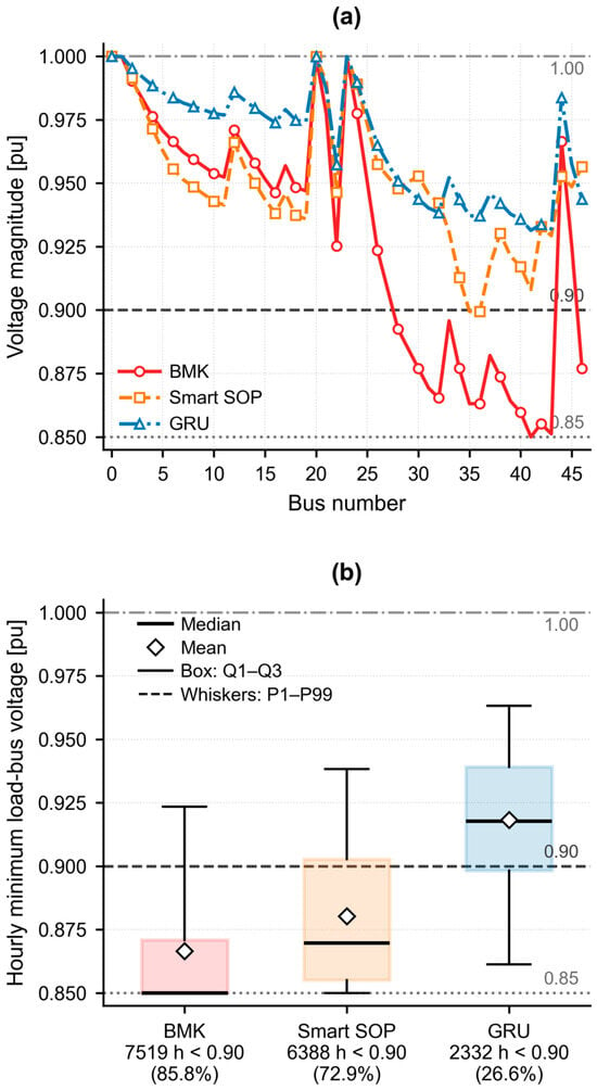
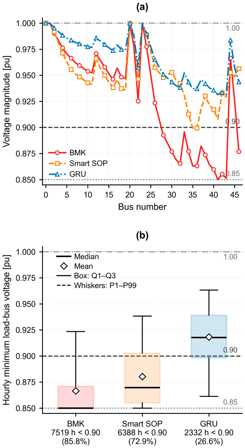
For the principal 1.5L + 200 EV case, BMK reaches the 0.85 pu feasibility limit at bus 41 during hour 2364. At the same hour, Smart SOP raises the minimum voltage to 0.8994 pu and GRU to 0.9314 pu (Figure 3a).
Figure 3.
Voltage performance under 1.5L + 200 EV: (a) load-bus voltages at the BMK worst hour (h = 2364); (b) annual hourly minimum-voltage distributions. Lines mark 0.85 pu feasibility, 0.90 pu reporting, and 1.00 pu nominal voltage.
As shown in Figure 3b, across the year, mean hourly minimum voltage is 0.8665, 0.8803, and 0.9182 pu for BMK, Smart SOP, and GRU; medians are 0.8500, 0.8697, and 0.9178 pu. Hours with any load-bus voltage below 0.90 pu fall from 7519 (85.8%) to 6388 (72.9%) and 2332 (26.6%), while affected load-bus-hours fall from 50,761 to 36,469 and 11,453. Smart SOP therefore reduces both duration and spatial extent of undervoltage, although GRU remains strongest.
4.2. Transformer Loading, Smart SOP Operation, and Demand-Side Flexibility
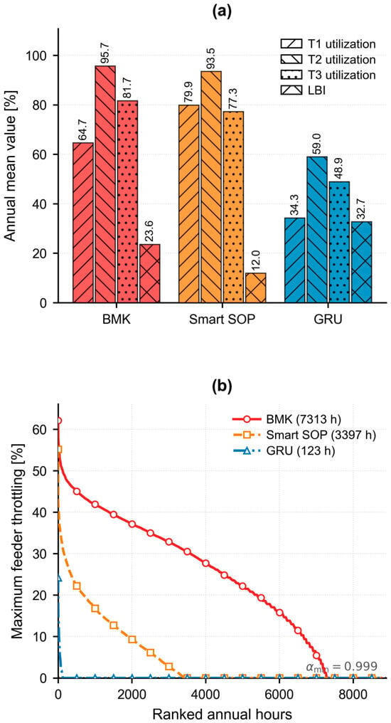
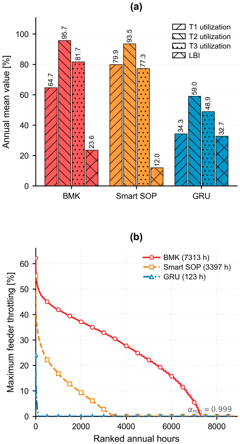
BMK mean transformer utilization is 64.7%, 95.7%, and 81.7% for T1–T3, giving a 23.6% mean LBI (Figure 4a). Smart SOP redistributes loading to 79.9%, 93.5%, and 77.3% and lowers mean LBI to 12.0% (−49.3%). GRU lowers utilization to 34.3%, 59.0%, and 48.9% but raises mean LBI to 32.7% because additional capacity does not change the spatial demand pattern.
Figure 4.
Transformer loading and demand-side flexibility under 1.5L + 200 EV: (a) annual mean transformer utilization and LBI; (b) annual duration curve of maximum feeder throttling.
Smart SOP operates throughout the year: maximum terminal active transfer is 167.8 kW, mean active transfer is 97.6 kW, and terminal mean utilization is 78.4%, 72.0%, and 64.1%. Aggregate reactive support averages 187.0 kVAr, peaks at 296.0 kVAr, and converter losses are 8.77 MWh/year.
Hours with more than 5% service reduction α < 0.95 fall from 7059 for BMK to 2670 for Smart SOP and 54 for GRU; for severe reduction α < 0.80, the values are 5392, 689, and 3 h. The any-intervention threshold α < 0.999 gives 7313, 3397, and 123 h, respectively. Mean throttling drops from 23.6% to 5.0% with Smart SOP, although the worst-hour maximum remains 55.2% (Figure 4b).
4.3. Annual Technical Performance
Table 2 summarizes annual technical performance. Smart SOP reduces ENS from 983.8 to 238.2 MWh (15.36% to 3.72%) and raises energy served from 5422.4 to 6167.9 MWh. GRU serves 6403.7 MWh and limits ENS to 2.4 MWh (0.04%). Smart SOP also lowers mean/max LBI from 23.57%/52.10% to 11.96%/33.25%, whereas GRU gives 32.72%/68.89%. Mean system power factor rises from 0.939 in BMK to 0.993 with Smart SOP (GRU: 0.943). Annual losses are 435.8, 541.3, and 314.6 MWh for BMK, Smart SOP, and GRU. The higher Smart SOP loss energy accompanies substantially greater energy delivery and converter/circulation losses. The optimized aggregate SOP rating is 0.402 MVA.
Table 2.
Main annual technical results under 1.5L + 200 EV.
4.4. Annualized Economic Performance
Table 3 shows that CAPEX is USD 465,238 for BMK, USD 521,368 for Smart SOP, and USD 930,477 for GRU. Annual system costs are USD 90,394, 106,130, and 152,940/year, respectively. Energy revenue is USD 271,120, 308,397, and 320,187/year. Despite its higher cost than BMK, Smart SOP gives the highest annual net value: USD 202,267/year versus USD 180,726 for BMK and USD 167,247 for GRU.
Table 3.
Annualized economic performance under 1.5L + 200 EV.
Annualized distribution cost is USD 0.0167/kWh for BMK, USD 0.0172/kWh for Smart SOP, and USD 0.0239/kWh for GRU. TVOLL, reported separately from utility cash flow, falls from USD 9.84 million/year in BMK to USD 2.38 million with Smart SOP and USD 24,275 with GRU.
4.5. Performance Across Load-Growth Scenarios
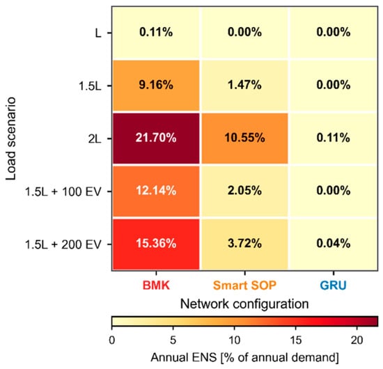
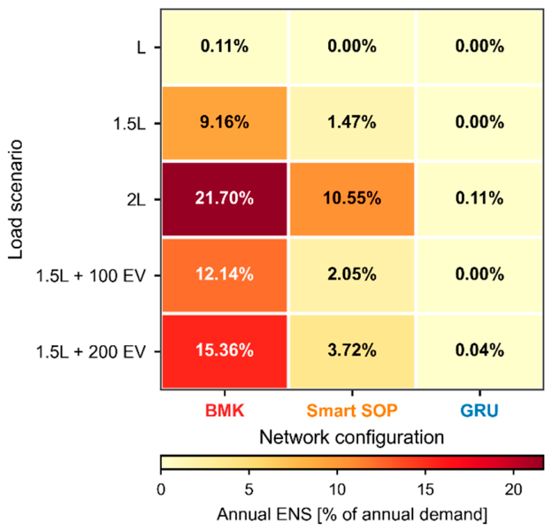
Across load scenarios, ENS [%] for BMK/Smart SOP/GRU is 0.11/0.00/0.00 at L; 9.16/1.47/0.00 at 1.5L; 21.70/10.55/0.11 at 2L; 12.14/2.05/0.00 at 1.5L + 100 EV; and 15.36/3.72/0.04 at 1.5L + 200 EV (Figure 5). The cross-scenario comparison therefore focuses on ENS as the common adequacy indicator. Detailed voltage, transformer-loading, and economic metrics are not repeated for every scenario because the purpose of the additional cases is to test the persistence of the network ranking rather than to redefine the principal planning case. The results show that Smart SOP consistently lies between BMK and GRU in supply adequacy, with its relative benefit greatest when feeder loading remains sufficiently complementary for inter-feeder power transfer.
Figure 5.
Annual ENS across load scenarios and network configurations; cells show ENS as a percentage of annual demand.
Smart SOP provides its strongest relative benefit when growth is substantial but uneven and complementary feeder capacity remains available. Its adequacy benefit declines at 2L because simultaneous system-wide growth reduces transferable spare capacity.
4.6. Smart SOP Capacity Sensitivity
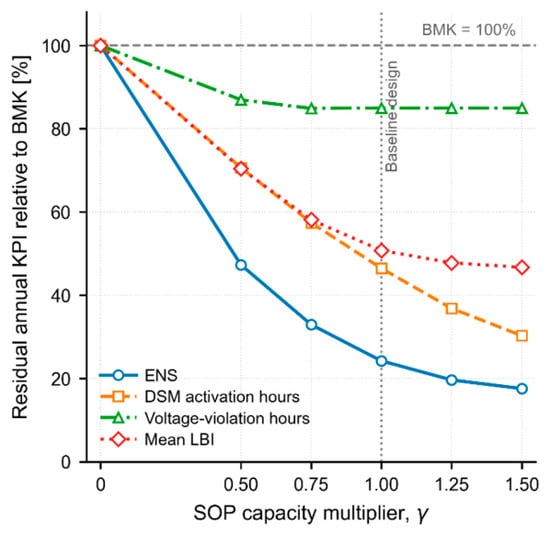
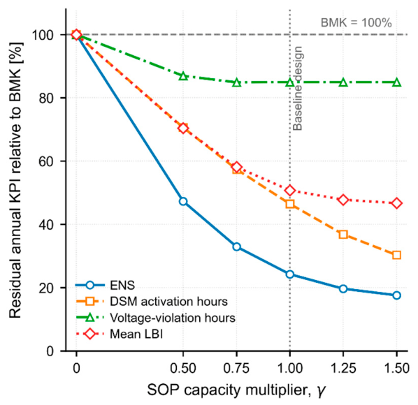
SOP capacity is scaled by γ, where γ = 0 is BMK, γ = 1 is the optimized baseline, and γ = 1.5 adds 50% capacity. At γ = 0.50, residual ENS, DSM activation hours, and mean LBI are 47.3%, 70.6%, and 70.4% of BMK; at γ = 0.75, they are 32.9%, 57.4%, and 58.1%. At γ = 1, the corresponding values are 24.2%, 46.5%, and 50.7%; at γ = 1.5, ENS and DSM hours fall to 17.6% and 30.3%, while LBI reaches 46.7%.
The curves show in Figure 6 diminishing returns beyond the baseline rating. Voltage-violation hours saturate earliest, remaining near 85% of BMK beyond γ ≈ 0.75, indicating that residual undervoltage is increasingly governed by feeder impedance and coincident loading rather than converter capacity.
Figure 6.
Annual technical indicators versus Smart SOP capacity multiplier γ under 1.5L + 200 EV, normalized to BMK.
4.7. Robustness Under Load Uncertainty
The economic robustness of the three network configurations was evaluated using 1000 stratified samples of the annual load multiplier
bounded to
λ∼(1.0, 0.102),
0.8 ≤ λ ≤ 1.2.
The multiplier is applied to the complete 1.5L + 200 EV annual profile, representing uncertainty in overall loading level rather than independent hourly variation.
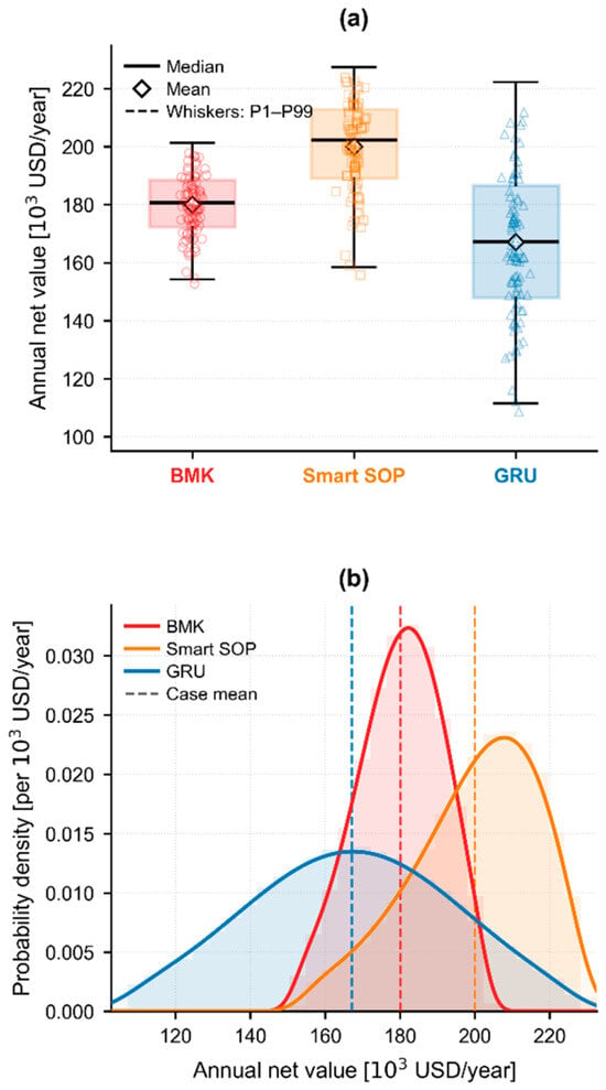
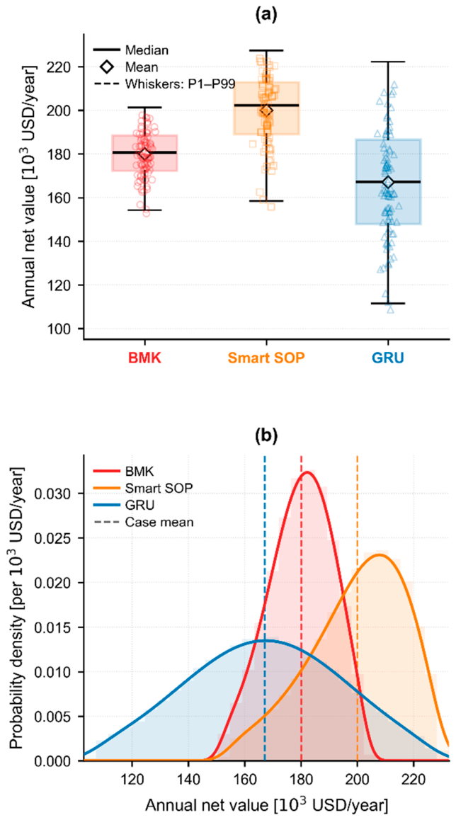
As shown in Figure 7, Smart SOP has the highest median annual net value at USD 202,268/year, versus USD 180,727 for BMK and USD 167,248 for GRU; means are USD 199,992, 180,076, and 167,149/year. Its interquartile range is USD 189,117–212,957/year, compared with USD 172,307–188,524/year for BMK and USD 147,905–186,555/year for GRU.
Figure 7.
Monte Carlo annual net value under load uncertainty: (a) boxplots; (b) distributions for BMK, Smart SOP, and GRU from 1000 samples with λ ~ N(1.0, 0.102), bounded by 0.8 ≤ λ ≤ 1.2.
Smart SOP has an 8.35% coefficient of variation and a minimum annual net value of USD 153,932/year, compared with 6.24% and USD 151,556 for BMK. GRU is the most utilization-sensitive, with a 15.9% coefficient of variation, a USD 26,580/year standard deviation, and a USD 106,543/year minimum. Mean ENS is 15.26% for BMK, 4.26% for Smart SOP, and 0.066% for GRU.
5. Discussion
5.1. Technical and Planning Implications
The results position Smart SOP primarily as a means of redistributing existing capacity before conventional reinforcement becomes unavoidable. Under 1.5L + 200 EV, Smart SOP lowers mean LBI from 23.57% to 11.96% by using spare capacity on less-stressed feeders, whereas GRU lowers absolute loading but leaves the spatial imbalance largely unchanged. This extends established multi-terminal balancing and capacity-value findings [6,9,10] to a full-year LV electrification case, consistent with recent EV-SOP planning studies [18,19].
Voltage performance also exposes the limit of this flexibility. Smart SOP improves the BMK worst-hour minimum from 0.8500 to 0.8994 pu and reduces annual undervoltage exposure, but larger converter ratings provide little additional reduction in violation hours. Once transfer capacity is sufficient, feeder impedance and coincident loading dominate; Smart SOP should therefore complement, not universally replace, conductor reinforcement [12].
Scenario and sizing results support this reinforcement-deferral interpretation. Smart SOP is highly effective at 1.5L, and EV-driven cases where feeder loading remains complementary, but ENS rises to 10.55% at 2L as system-wide growth removes spare capacity. Capacity sensitivity shows diminishing returns beyond the 0.402 MVA baseline [14,20,21].
5.2. Economic Performance and Uncertainty
The service and economic results show the central trade-off. Smart SOP reduces ENS from 15.36% to 3.72%, while GRU nearly eliminates ENS at 0.04%. However, GRU’s higher fixed investment reduces annual net value. Smart SOP recovers 745.5 MWh/year of otherwise unserved energy and reaches USD 202,267/year net value, exceeding both BMK and GRU. Its higher loss energy reflects both greater energy delivery and converter/circulation losses [15].
The economic ranking was also checked against key financial assumptions while keeping technical results unchanged. Smart SOP remains the highest annual-net-value option for discount rates of 5–15%, energy values of USD 0.03–0.08/kWh, OPEX of 1–5% of CAPEX, and passive/SOP-electronics lifetimes of 15/8 to 30/15 years. Its annual net value spans approximately USD 89,733–371,063/year across these one-at-a-time tests, showing that absolute values are assumption-dependent while the ranking is preserved.
The Monte Carlo assessment gives Smart SOP the highest mean and median annual net value under the considered load uncertainty. GRU has the largest coefficient of variation and lowest minimum value because more capital is committed before demand is realized, highlighting the value of flexibility under uncertain EV-driven growth [16,17,18,19].
5.3. Limitations and Generalizability
The reported ranking is demonstrated for the modified CIGRE LV benchmark and may vary with topology, feeder impedance, phase imbalance, EV/load distribution, and available spare capacity. The balanced steady-state model excludes neutral effects, harmonics, converter dynamics, faults, protection, and communication or measurement delays. The served-load variable α represents aggregate feeder-level service flexibility rather than explicit customer demand–response behavior. GRU is a standardized duplicated transformer/feeder benchmark; actual reinforcement designs and costs may differ.
The uncertainty study varies aggregate loading while retaining a fixed EV population, usage-class allocation, and charging-profile realization, and uses a reduced feeder-routing model rather than repeated full 8760-h nonlinear optimization. Future work should include uncertainty in EV penetration, charging location, usage-class composition, and behavior.
Within these limits, Smart SOP is most attractive when demand growth is rapid and spatially uneven and complementary feeder capacity remains available. When growth becomes uniformly severe or voltage and reliability requirements dominate, conventional reinforcement remains necessary.
6. Conclusions
This study evaluated a three-terminal Smart SOP as a reinforcement-deferral option for an LV network exposed to rapid load growth and transport electrification using 8760-h nonlinear AC optimization, independent pandapower validation, multiple load cases, capacity sensitivity, and load uncertainty.
Under 1.5L + 200 EV, Smart SOP reduces ENS from 15.36% to 3.72%, increases energy served from 5422.4 to 6167.9 MWh, lowers mean LBI from 23.57% to 11.96%, and reduces hours with more than 5% service reduction from 7059 to 2670. GRU provides the strongest technical performance, limiting ENS to 0.04%, but its higher capital and annualized costs produce a lower annual net value.
Smart SOP achieves the highest annual net value at USD 202,267/year, compared with USD 180,726 for BMK and USD 167,247 for GRU. Capacity sensitivity shows diminishing returns beyond the 0.402 MVA baseline, while Monte Carlo analysis gives Smart SOP the highest mean and median annual net value under uncertain loading. These results support Smart SOP as a non-wire reinforcement-deferral strategy for rapid, uneven demand growth where complementary feeder capacity remains available; conventional reinforcement remains necessary when system-wide loading becomes uniformly severe or voltage and reliability requirements dominate.
Author Contributions
Methodology, P.O.E., E.O., and E.D.; software, E.O.; validation, E.O.; formal analysis, E.O. and E.D.; data curation, E.O.; writing—original draft preparation, E.O.; writing—review and editing, P.O.E., E.O., and E.D.; visualization, E.O. All authors have read and agreed to the published version of the manuscript.
Funding
This research received no external funding.
Data Availability Statement
The building-load profiles are publicly available from the Open Energy Data Initiative dataset cited in [28]. EV charging profiles and simulation outputs generated in this study are available from the corresponding author upon reasonable request.
Acknowledgments
During preparation of this manuscript, the authors used OpenAI ChatGPT (GPT-5.6) for language refinement. The authors reviewed and edited the output and take full responsibility for the content.
Conflicts of Interest
The authors declare no conflicts of interest.
Abbreviations
| BMK | Unreinforced benchmark network |
| CAPEX | Capital expenditure |
| DSM | Demand-side management/service intervention |
| ENS | Energy not served |
| ES | Energy served |
| EV | Electric vehicle |
| GRU | Conventional grid reinforcement |
| LBI | Load-balancing index |
| LV | Low voltage |
| OPEX | Operating expenditure |
| PF | Power factor |
| SOP | Soft open point |
| VOLL | Value of lost load |
| TVOLL | Total value of lost load |
| αf,h | Fraction of feeder f demand served at hour h |
| βi | SOP terminal sizing variable |
| γ | SOP-capacity sensitivity multiplier |
| λ | Annual load uncertainty multiplier |
| P, Q | Active and reactive power |
| V, θ | Voltage magnitude and phase angle |
| FV | Voltage-deviation objective term |
| FENS | Curtailed-energy objective term |
| Floss | Network-loss objective term |
| Fβ | SOP-capacity objective term |
| FSOP | SOP-operation regularization term |
| wV, wα, wloss, wβ, wSOP | Objective weighting coefficients |
| Δt | Simulation time step |
References
- International Energy Agency. Global EV Outlook 2025; IEA: Paris, France, 2025. [Google Scholar]
- Qian, K.; Zhou, C.; Allan, M.; Yuan, Y. Modeling of load demand due to EV battery charging in distribution systems. IEEE Trans. Power Syst. 2011, 26, 802–810. [Google Scholar] [CrossRef] [Scilit]
- Leou, R.-C.; Su, C.-L.; Lu, C.-N. Stochastic analyses of electric vehicle charging impacts on distribution network. IEEE Trans. Power Syst. 2014, 29, 1055–1063. [Google Scholar] [CrossRef] [Scilit]
- Athanasiadis, C.L.; Papadopoulos, T.A.; Kryonidis, G.C.; Pippi, K.D. A benchmarking testbed for low-voltage active distribution network studies. IEEE Open Access J. Power Energy 2023, 10, 104–115. [Google Scholar] [CrossRef] [Scilit]
- Deakin, M.; Sarantakos, I.; Greenwood, D.M.; Bialek, J.W.; Taylor, P.C.; Ming, W.; Patsios, C. Hybrid open points: An efficient tool for increasing network capacity in distribution systems. IEEE Trans. Power Deliv. 2022, 37, 1340–1343. [Google Scholar] [CrossRef] [Scilit]
- Jiang, X.; Zhou, Y.; Ming, W.; Yang, P.; Wu, J. An overview of soft open points in electricity distribution networks. IEEE Trans. Smart Grid 2022, 13, 1899–1910. [Google Scholar] [CrossRef] [Scilit]
- Cao, W.; Wu, J.; Jenkins, N.; Wang, C.; Green, T. Operating principle of soft open points for electrical distribution network operation. Appl. Energy 2016, 164, 245–257. [Google Scholar] [CrossRef] [Scilit]
- Wang, C.; Song, G.; Li, P.; Ji, H.; Zhao, J.; Wu, J. Optimal siting and sizing of soft open points in active electrical distribution networks. Appl. Energy 2017, 189, 301–309. [Google Scholar] [CrossRef] [Scilit]
- Sarantakos, I.; Zografou-Barredo, N.-M.; Huo, D.; Greenwood, D.M. A reliability-based method to quantify the capacity value of soft open points in distribution networks. IEEE Trans. Power Syst. 2021, 36, 5032–5043. [Google Scholar] [CrossRef] [Scilit]
- Ji, H.; Wang, C.; Li, P.; Zhao, J.; Song, G.; Ding, F.; Wu, J. An enhanced SOCP-based method for feeder load balancing using the multi-terminal soft open point in active distribution networks. Appl. Energy 2017, 208, 986–995. [Google Scholar] [CrossRef] [Scilit]
- Li, P.; Ji, H.; Wang, C.; Zhao, J.; Song, G.; Ding, F.; Wu, J. Optimal operation of soft open points in active distribution networks under three-phase unbalanced conditions. IEEE Trans. Smart Grid 2019, 10, 380–391. [Google Scholar] [CrossRef] [Scilit]
- Favre-Perrod, P.; Auberson, E.; Bernasconi, C.; Demierre, A.; Gavin, S.; Carpita, M.; Bifrare, A. Application of soft-open points for the interconnection of neighbouring low voltage distribution networks. IET Conf. Proc. 2021, 2021, 1076–1080. [Google Scholar] [CrossRef] [Scilit]
- Hou, Q.; Dai, N.; Huang, Y. Voltage regulation enhanced hierarchical coordinated Volt/Var and Volt/Watt control for active distribution networks with soft open points. IEEE Trans. Sustain. Energy 2024, 15, 2021–2037. [Google Scholar] [CrossRef] [Scilit]
- Deakin, M. Multiplexing power converters for cost-effective and flexible soft open points. IEEE Trans. Smart Grid 2024, 15, 260–271. [Google Scholar] [CrossRef] [Scilit]
- Deakin, M.; Sarantakos, I.; Greenwood, D.; Bialek, J.; Taylor, P.C.; Walker, S. Comparative analysis of services from soft open points using cost-benefit analysis. Appl. Energy 2023, 333, 120618. [Google Scholar] [CrossRef] [Scilit]
- Shen, Y.; Zhang, S.; Ding, M.; Cheng, H.; Li, C.; Liu, D. Expansion planning of soft open points based distribution system considering EV traffic flow. IEEE Trans. Ind. Appl. 2024, 60, 1229–1239. [Google Scholar] [CrossRef] [Scilit]
- Yang, X.; Xu, C.; Zhang, Y.; Yao, W.; Wen, J.; Cheng, S. Real-time coordinated scheduling for ADNs with soft open points and charging stations. IEEE Trans. Power Syst. 2021, 36, 5486–5499. [Google Scholar] [CrossRef] [Scilit]
- Fang, J.; Li, W.; Chen, D. Electric vehicle and soft open points co-planning for active distribution grid flexibility enhancement. Energies 2025, 18, 694. [Google Scholar] [CrossRef] [Scilit]
- Zheng, C.; Dai, Q.; Chen, Z.; Peng, J.; Guo, G.; Lin, D.; Ye, Q. Application of mobile soft open points to enhance hosting capacity of EV charging stations. Energies 2025, 18, 5758. [Google Scholar] [CrossRef] [Scilit]
- Cheng, Q.; Li, X.; Zhang, M.; Fei, F.; Shi, G. Optimal configuration strategy of soft open point in flexible distribution network considering reactive power sources. Energies 2025, 18, 529. [Google Scholar] [CrossRef] [Scilit]
- Pang, D.; Wang, Z.; Shi, X.; Ge, J.; Wang, Z.; Yi, H.; Zhuang, Y.; Yin, Y.; Wang, W. Multi-level dynamic weight optimization scheduling strategy for flexible interconnected distribution substations based on three-port SNOPs. Energies 2025, 18, 2421. [Google Scholar] [CrossRef] [Scilit]
- Tian, X.; Cai, Y.; Sun, X.; Zhu, Z.; Wang, Y.; Xu, Y. Incorporating driving style recognition into MPC for energy management of plug-in hybrid electric buses. IEEE Trans. Transp. Electrif. 2023, 9, 169–181. [Google Scholar] [CrossRef] [Scilit]
- Tian, X.; Wan, M.; Chen, X.; Cai, Y.; Sun, X.; Zhu, Z. Driver-oriented adaptive equivalent consumption minimization strategy for plug-in hybrid electric buses. Energies 2025, 18, 5033. [Google Scholar] [CrossRef] [Scilit]
- Hu, C.; Zhang, X.; Wu, Q. Collaborative active and reactive power control of DERs for voltage regulation and frequency support by distributed event-triggered heavy ball method. IEEE Trans. Smart Grid 2023, 14, 3804–3815. [Google Scholar] [CrossRef] [Scilit]
- CIGRE Task Force C6.04.02. Benchmark Systems for Network Integration of Renewable and Distributed Energy Resources; CIGRE Technical Brochure 575; CIGRE: Paris, France, 2014. [Google Scholar]
- Bynum, M.L.; Hackebeil, G.A.; Hart, W.E.; Laird, C.D.; Nicholson, B.L.; Siirola, J.D.; Watson, J.-P.; Woodruff, D.L. Pyomo-Optimization Modeling in Python, 3rd ed.; Springer: Cham, Switzerland, 2021. [Google Scholar] [CrossRef] [Scilit]
- Thurner, L.; Scheidler, A.; Schäfer, F.; Menke, J.-H.; Dollichon, J.; Meier, F.; Meinecke, S.; Braun, M. Pandapower-An open-source Python tool for convenient modeling, analysis, and optimization of electric power systems. IEEE Trans. Power Syst. 2018, 33, 6510–6521. [Google Scholar] [CrossRef] [Scilit]
- Ong, S.; Clark, N. Commercial and Residential Hourly Load Profiles for All TMY3 Locations in the United States; Open Energy Data Initiative (OEDI), National Renewable Energy Laboratory: Golden, CO, USA, 2014. [Google Scholar] [CrossRef] [Scilit] [PubMed]
- Ma, Y.; Tao, J.; Xu, Y.; Hu, H.; Liu, G.; Qin, T.; Fu, X.; Liu, R. Multi-mode operation and coordination control strategy based on energy storage and flexible multi-state switch for the new distribution network during grid-connected operation. Energies 2025, 18, 3389. [Google Scholar] [CrossRef] [Scilit]
- Sun, F.; Ma, J.; Yu, M.; Wei, W. Optimized two-time scale robust dispatching method for the multi-terminal soft open point in unbalanced active distribution networks. IEEE Trans. Sustain. Energy 2021, 12, 587–598. [Google Scholar] [CrossRef] [Scilit]
- Wächter, A.; Biegler, L.T. On the implementation of an interior-point filter line-search algorithm for large-scale nonlinear programming. Math. Program. 2006, 106, 25–57. [Google Scholar] [CrossRef] [Scilit]
- Billinton, R.; Allan, R.N. Reliability Evaluation of Power Systems, 2nd ed.; Plenum Press: New York, NY, USA, 1996. [Google Scholar]
- Farzamnia, A.; Marjani, S.; Galvani, S.; Kin, K.T.T. Optimal allocation of soft open point devices in renewable energy integrated distribution systems. IEEE Access 2022, 10, 9309–9320. [Google Scholar] [CrossRef] [Scilit]

Disclaimer/Publisher’s Note: The statements, opinions and data contained in all publications are solely those of the individual author(s) and contributor(s) and not of MDPI and/or the editor(s). MDPI and/or the editor(s) disclaim responsibility for any injury to people or property resulting from any ideas, methods, instructions or products referred to in the content. |
© 2026 by the authors. Licensee MDPI, Basel, Switzerland. This article is an open access article distributed under the terms and conditions of the Creative Commons Attribution (CC BY) license.