


Abstract
China’s National Big Data Comprehensive Pilot Zones (BDPZs) constitute one of the world’s largest place-based digital economy experiments. This paper provides the first county-level evaluation of the program, asking whether the designation shifted local economies from secondary toward tertiary activity—a structural margin relevant to, but distinct from, energy transition. Using panel data on 1592 counties (2011–2023) and a matched staggered difference-in-differences design, we combine exact two-way fixed-effects estimation with the heterogeneity-robust estimators of Callaway and Sant’Anna (2021) and Sun and Abraham (2021), formal joint pre-trend tests, randomization inference, relative-magnitude sensitivity bounds, and spillover falsification. Our central result is a delayed shift in the nominal value-added structure toward services in the 2017 adoption cohort: the effect is statistically indistinguishable from zero for three years, then builds to +4.9, +6.7, and +10.6 percentage points in post-treatment years four through six (all ), is robust across never-treated, matched, distant, and growth-trajectory-matched control sets, and survives a conservative relative-magnitude sensitivity bound (breakdown ) despite a formally rejected parallel-trends test. Three qualifications discipline the reading. First, the shift appears in value-added shares but not in (incompletely measured) employment shares, consistent with a price- and productivity-driven value-composition change rather than labor reallocation. Second, per capita income did not rise—it fell relative to poorer, faster-converging controls—so we make no growth claim. Third, the single-province 2016 (Guizhou) case is not separately identified: its sign flips across control sets, and it is statistically indistinguishable from province-level placebos (), so we set it aside. Because sectoral recomposition bears on energy intensity (under constant sectoral intensities) but not on energy sources or absolute use—and because data-center construction is itself energy-intensive—we make no energy-transition claim; the net energy effect is sign-indeterminate with current data.
1. Introduction
China has committed to peaking carbon emissions before 2030 and reaching carbon neutrality by 2060. These targets demand not only changes in the energy mix but also a reconfiguration of the economic structure underlying energy demand [1,2]. Because the tertiary sector consumes far less energy per unit of value added than heavy manufacturing [3,4], the sectoral composition of economic activity is one of the structural margins on which any energy transition ultimately rests. It is, however, only one margin: energy transition in the strict sense refers to changes in energy sources, renewable adoption, energy efficiency, and decarbonization outcomes [5,6], and a sizable literature warns that growth in cleaner or less energy-intensive activities frequently adds to, rather than displaces, existing energy demand [7,8,9]. This paper is, therefore, explicit about its object of study: we estimate the effect of a major place-based digital economy policy on the county-level shift from secondary to tertiary industry—structural transformation—and we treat the implications for energy transition as exactly that: implications, to be drawn cautiously and tested directly only when county-level energy data permit.
The policy we study is the National Big Data Comprehensive Pilot Zones (BDPZs). Starting in 2015, China’s State Council designated selected provinces and city clusters as experimental areas for big data infrastructure construction, cross-sectoral data sharing, and digital industry development. The first batch (Guizhou province, effective 2016) and the second batch (Beijing–Tianjin–Hebei, Shanghai, Henan, Chongqing, Inner Mongolia, the Pearl River Delta in Guangdong, and Shenyang in Liaoning, effective 2017) created a staggered treatment structure suitable for difference-in-differences (DID) analysis. A growing literature evaluates the BDPZ program at the prefecture level, generally finding favorable effects on carbon intensity, energy conservation, and low-carbon development [10,11,12,13], though recent work also documents conflicting mechanisms, with digital infrastructure construction itself raising local energy demand [14,15].
This paper makes three contributions to that literature. First, identification discipline: to our knowledge, this is the first BDPZ evaluation to deploy the complete modern staggered-DID toolkit—exact two-way fixed-effects (TWFEs) estimation, the heterogeneity-robust estimators of Callaway and Sant’Anna [16] and Sun and Abraham [17], formal joint pre-trend tests [18], relative-magnitude sensitivity analysis [19], randomization inference, coefficient-stability bounds [20], and explicit spillover falsification tests—and our findings show that the discipline matters: prefecture-level favorable estimates do not all survive it at finer geography. Indeed, we document that the popular one-step demeaning approximation to TWFE inflates the static estimate roughly threefold in our unbalanced panel, a methodological caution of independent interest. Second, granularity with cohort transparency: county-level data (1592 counties, finer than the prefecture data used in nearly all prior BDPZ studies) reveal that the pooled average is a misleading summary—it nets a robust positive 2017 adoption cohort against a single-province 2016 (Guizhou) case that is not separately identified. Third, honest framing: we do not equate sectoral recomposition with energy transition. Our outcome is a structural transformation index (STI) built from sectoral value-added shares; we test it against employment shares, document why county-level energy quantities cannot support direct outcome tests, and bound what our estimates can and cannot say about energy—which, we conclude, is little.
Our central finding is a robust but narrow one. Isolating the 2017 adoption cohort—the object on which clean never-treated comparisons identify a treatment effect—designation is followed by a pronounced delayed shift in the nominal value-added structure toward services: the event-study coefficients are near zero for three years and then build monotonically to , , and percentage points in years four through six (all ), with a Callaway–Sant’Anna (CS) overall post-treatment effect of percentage points (). This effect is robust across never-treated, propensity-matched, geographically distant, and pre-growth-trajectory-matched control sets, and although formal joint tests reject strict parallel trends, the late effect survives a conservative relative-magnitude sensitivity bound in the spirit of Rambachan and Roth [19], with a breakdown value for the year five–six average (Section 7). The pooled estimate across both cohorts is far smaller (– percentage points; matched CS ) because it averages this positive cohort against the 2016 case.
Three qualifications, each established by a dedicated test, keep the interpretation honest. First, the value-added shift is not mirrored in employment shares: the same design applied to the (admittedly incomplete) formal-employment data yields a null for the 2017 cohort, consistent with a price- and productivity-driven composition change rather than a reallocation of labor (Section 8). Second, per capita income did not rise—in the developed 2017 cohort, it fell relative to poorer never-treated controls, a pattern we trace to conditional convergence rather than to the policy, and which leaves the structural result intact under growth-trajectory matching. Third, the 2016 “cohort” is the single province of Guizhou (78 counties): its estimate flips sign across control sets and is statistically indistinguishable from province-level placebos (p = 0.27), so we treat it as not separately identified and decline to interpret it as a second “policy.” We had, in an earlier draft, read the Guizhou negative as an infrastructure-led channel; the placebo evidence does not support that reading, and we withdraw it.
Two further design features discipline the language throughout. BDPZ designation was not random; propensity score matching (PSM) and coefficient-stability bounds [20] address observable and proportional-unobservable selection but cannot exclude residual selection. And spillovers are real: never-treated counties in provinces bordering pilot provinces both tertiarized and de-industrialized after 2017—the latter inconsistent with manufacturing relocating to neighbors but indicative of regional co-movement that we cannot fully separate from diffusion (Section 7). For all these reasons, we describe our estimates as policy-associated changes, consistent with a causal reading under stated assumptions, and we flag every place where the evidence falls short of that standard.
The remainder of this paper proceeds as follows. Section 2 reviews related literature and states hypotheses. Section 3 develops a two-sector general equilibrium model that formalizes the structural channel and derives testable predictions. Section 4 describes the BDPZ institutional setting, including concrete examples of policy implementation. Section 5 presents the identification strategy, estimators, and an explicit discussion of methodological limitations. Section 6 details the data and variables. Section 7 reports baseline results, dynamic estimates, and robustness checks. Section 8 examines intermediate outcomes. Section 9 explores heterogeneity. Section 10 returns to each hypothesis, draws tempered policy implications, and concludes.
2. Literature Review and Hypotheses
2.1. Digitalization, Structural Change, and Energy Demand
The conceptual foundation for our analysis rests on the proposition that digital technologies reshape the sectoral composition of economic activity, with consequences for aggregate energy intensity. In the canonical view, digital infrastructure functions as a general-purpose technology whose diffusion lowers the cost of information-intensive activities relative to material-intensive ones [21,22]. As a result, the comparative advantage of sectors amenable to digitalization—typically services, knowledge-intensive manufacturing, and platform commerce—rises at the expense of less adaptable sectors such as heavy industry. Empirically, this composition mechanism has been documented in studies of Chinese cities: Hao et al. [23] find that digitalization stimulates green economic growth primarily through industrial structure optimization, while Ma and Lin [24] document a synergistic effect of digitalization and industrialization on energy savings.
A second strand examines the direct effect of digital infrastructure on energy demand. The evidence is mixed. Hao et al. [25] find that internet development reduces electricity intensity in China, Ren et al. [26] document that internet penetration lowers per capita energy consumption, and Wu et al. [4] and Song et al. [3] provide evidence that the digital economy enhances energy efficiency. Against this, the information and communication technology sector is itself energy-intensive [14], digitalization can induce rebound effects through expanded consumption [27,28], and recent evidence on China’s big data policy specifically documents conflicting mechanisms: Zhou et al. [15] show that the digital infrastructure construction triggered by the BDPZ program raises local energy demand even as other channels reduce emissions. Sun et al. [29] similarly emphasize that low-carbon effects of the digital economy in Chinese cities operate through innovation and efficiency channels whose net energy balance is an empirical question.
A third strand focuses on carbon outcomes of digitalization more broadly [30,31,32,33], and on the energy transition specifically [34,35,36,37,38].
2.2. Evaluations of the BDPZ Program
A rapidly growing quasi-experimental literature evaluates the BDPZ program itself, almost exclusively at the prefecture level. Pan et al. [12] find that pilot designation reduced urban carbon emissions; Liu et al. [11] document carbon reductions operating through green innovation, energy structure, and capital allocation channels; Shen and Wang [13] show that digital industrialization promoted urban energy conservation through industrial upgrading; and Liu and Xiao [10] report low-carbon development effects that are strongest in the central region. Two features of this literature motivate our contribution. First, prefecture-level aggregation masks the within-prefecture heterogeneity in industrial structure that determines where structural transformation can occur; we move to the county level. Second, most studies rely on conventional TWFE estimation, which recent econometric work shows can be severely biased under staggered adoption with dynamic effects [39,40]; we deploy the modern toolkit and document, transparently, how much the answers change.
2.3. Energy Transitions, Energy Additions, and the Structural Margin
An influential line of work cautions against equating growth in cleaner or less energy-intensive activity with energy transition. York [8] shows that, historically, alternative energy sources have displaced remarkably little fossil fuel use; York and Bell [9] argue that observed “transitions” have more often been energy additions, with new sources and sectors stacking on top of old ones; and Fressoz [7] documents at length that the history of energy is a history of accumulation rather than substitution. Saito [41] makes a related theoretical argument that decoupling through sectoral change tends to displace, rather than eliminate, material and energy throughput. Applied to our setting, these critiques imply two distinct concerns: (i) a rising tertiary share need not reduce total energy use, even locally, if service growth comes on top of—rather than instead of—industrial activity, and if digital infrastructure itself consumes substantial energy; and (ii) a falling secondary share in pilot counties may partly reflect the relocation of industrial activity to other jurisdictions rather than its transformation. Our research design can speak to the composition margin within counties, and our spillover tests provide indirect evidence on relocation, but neither concern can be fully resolved with available data. We, therefore, define our outcome strictly as structural transformation and return to both concerns in Section 7 and Section 10.
2.4. Place-Based Policies and Staggered DID Methodology
A separate methodological strand uses quasi-natural experiments to identify place-based policy effects in China: smart city pilots [42,43,44], low-carbon city pilots [45], and central environmental inspections [46]. We build on this tradition while incorporating the recent econometric literature on staggered DID. Goodman-Bacon [40] and de Chaisemartin and D’Haultfœuille [39] show that static TWFE estimates are weighted averages that can place negative weights on some treatment effects when adoption is staggered and effects are dynamic; Callaway and Sant’Anna [16] and Sun and Abraham [17] propose estimators robust to this problem; Borusyak et al. [47] provide an efficient imputation alternative; Roth [18] demonstrates that conventional pre-trend tests have low power and that conditioning on passing them distorts inference; and Rambachan and Roth [19] develop partial identification methods when parallel trends is violated. Wolfers [48] provides the classic caution that unit-specific time trends absorb dynamically growing treatment effects. This toolkit structures our entire empirical analysis.
2.5. Hypotheses
Based on the literature reviewed above, three hypotheses emerge that we formalize in Section 3 and test empirically:
Hypothesis 1.
(Structural effect). BDPZ designation raises the tertiary industry share and lowers the secondary industry share of county GDP, raising the composite structural transformation index.
Hypothesis 2.
(Channels). The policy operates through three candidate channels: industrial composition change, income growth, and consumption upgrading. We test whether each intermediate outcome responds to the policy; we do not claim a formal mediation decomposition.
Hypothesis 3.
(Complementarity). The policy effect is amplified in counties with greater pre-existing economic capacity and industrial intensity, reflecting complementarity between digital infrastructure and traditional economic resources.
Section 3 embeds these hypotheses in a formal two-sector general equilibrium framework, and Section 10 returns to each hypothesis with an explicit verdict.
3. Theoretical Framework
To organize the empirical analysis and clarify the channels through which digital economy policy can affect economic structure—and, by implication, energy intensity—this section develops a parsimonious two-sector general equilibrium model. The framework formalizes three core insights: (i) digital infrastructure operates as a sector-biased productivity shock that disproportionately benefits the tertiary sector; (ii) the resulting structural reallocation would, holding sectoral energy intensities constant, reduce aggregate energy intensity through composition effects; and (iii) the magnitude of the structural effect depends on the pre-existing industrial composition, generating testable heterogeneity predictions. We emphasize at the outset that prediction (ii) concerns a quantity—aggregate energy intensity—that our county data cannot measure (Section 6); it is an implication of the structural predictions we do test, not itself a tested outcome.
3.1. Setup: A Two-Sector Economy with Energy as an Input
Consider a closed county economy producing two final goods: a manufacturing (secondary-sector) good, M, and a service (tertiary-sector) good, S. Each sector uses labor, L, and energy, E, as inputs, with sector-specific Cobb–Douglas technologies:
where and are sector-specific total factor productivities. The empirical regularity that manufacturing is more energy-intensive than services is captured by the assumption [3,4]. Total resources satisfy and , with L exogenously given and E obtained at unit price from an external supplier.
Representative households have CES preferences over the two goods:
where is the preference weight on manufactured goods, and is the elasticity of substitution between the two sectors. With , the two goods are gross substitutes—an empirically supported assumption for the secondary–tertiary margin in China [23].
3.2. Equilibrium and the Digitalization Shock
Profit-maximizing firms equate marginal revenue product to factor cost. With and denoting sector prices and w the wage, the first-order conditions yield factor demands:
where denotes sectoral output. Market clearing in goods, labor, and energy markets, combined with the CES demand structure, pins down the relative output ratio:
The digital infrastructure shock. We model the BDPZ policy as a positive shock to the tertiary-sector productivity , while leaving unchanged. (This modeling choice is motivated by the observation that big data infrastructure—cloud computing, data centers, e-commerce platforms—enables fundamentally new service activities (digital finance, platform commerce, online education) but offers more modest productivity gains in traditional heavy manufacturing [4,22]. It is a simplification: the construction phase of a data center buildout is itself an industrial activity, a point we return to when interpreting the negative western-region results in Section 9.
Under cost minimization with the Cobb–Douglas technology, the unit cost in sector j is for some constant, . In competitive equilibrium, , so a productivity shock to reduces proportionally:
3.3. Comparative Statics: Testable Predictions
The relative size of the service sector rises with the policy. The magnitude scales with the elasticity of substitution: when , structural reallocation is amplified. This delivers Hypothesis 1—the BDPZ policy raises the tertiary share and reduces the secondary share , raising the composite index .
Prediction 2
(Implied energy intensity reduction; not directly tested). The total energy use is , and the total output is . The aggregate energy intensity is, therefore:
where is the manufacturing value-added share. Differentiating with respect to the policy and using Prediction 1:
since by assumption and from Prediction 1. Aggregate energy intensity falls through a pure composition effect—with sectoral energy intensities being held constant. Two caveats make this an implication rather than a tested outcome. First, county-level energy quantities are too sparsely reported to support estimation (Section 6). Second, the assumption of constant sectoral intensities is substantive: if the policy simultaneously raises the energy intensity of the service sector itself (data centers are electricity-intensive [14,15]), or if displaced manufacturing relocates rather than disappears [8,9], realized energy outcomes can deviate substantially from (10). Section 10 quantifies the composition arithmetic under explicit assumptions.
Prediction 3
(Heterogeneity by initial industrial intensity). Differentiating Equation (10) a second time with respect to the initial manufacturing share :
To sign this cross-partial, note that a county fully specialized in services () has no manufacturing to reallocate from, so the absolute response must be increasing in for small initial shares. Formally, expressing in terms of and :
The Jacobian is maximized at and vanishes at . For counties with below this maximum, increasing raises the absolute response to a digital productivity shock. Consequently, the structural response is increasing in pre-treatment industrial intensity—at least for the empirically relevant range . This delivers Hypothesis 3: the policy effect is amplified in counties with greater initial industrial intensity.
Prediction 4
(Heterogeneity by initial economic capacity). The model can be extended to incorporate an absorptive-capacity friction. Suppose digital productivity gains require a complementary local input K (financial development, human capital, infrastructure), so that the realized productivity shock is with . Then:
Counties with higher initial K—approximated empirically by initial GDP per capita—experience larger structural shifts. Together with Prediction 3, this delivers Hypothesis 3.
3.4. Candidate Transmission Channels
The model also clarifies three candidate channels through which the policy may operate—each of which we examine empirically in Section 8 as an intermediate outcome, without claiming a formal mediation decomposition.
- Channel I: Structural reallocation. The sectoral reallocation derived in Prediction 1 is the most direct channel: the tertiary share rises and the secondary share falls.
- Channel II: Aggregate income. The policy raises real income because the tertiary productivity gain reduces the cost of the service good. Using the indirect utility function, the real per capita income, y, satisfies:where is the optimal expenditure share on manufacturing.
- Channel III: Consumption composition. Higher real income shifts consumption toward services if services are luxury goods (income elasticity ):where captures non-homotheticity. We caution that, even where consumption shifts toward services, the literature on energy rebound and energy additions implies no presumption that total household energy use falls [7,9,27]; we treat Channel III strictly as a statement about consumption composition.
3.5. Summary of Theoretical Predictions
Table 1 summarizes the model’s predictions and their mapping to the empirical analysis.
Table 1.
Summary of theoretical predictions.
Figure 1 synthesizes the mechanism: the policy intervention (left), three candidate channels (middle), and the structural transformation outcomes (right), with moderators capturing complementarity effects.
Figure 1.
Theoretical mechanism: from BDPZ designation to structural transformation outcomes. The BDPZ policy operates as a sector-biased productivity shock, , on tertiary-sector productivity , propagating through three candidate channels. Magnitudes in the right-hand column are the preferred Callaway–Sant’Anna estimates from Section 7 and Section 8. The implied decline in aggregate energy intensity (Prediction 2) is an interpretation conditional on stable sectoral energy intensities, not a directly tested outcome.
With the theoretical framework in place, we now describe the institutional setting of the BDPZ policy before turning to the empirical implementation.
4. Institutional Background
In September 2015, China’s State Council issued the “Action Outline for Promoting the Development of Big Data,” establishing the strategic framework for national big data development. The BDPZ program emerged as the primary vehicle for implementing this vision. The first pilot zone was approved in Guizhou province in October 2015, with implementation effective from 2016. Guizhou’s selection was strategic: its underdeveloped economy and cool climate (favorable for data center cooling) presented an opportunity to leapfrog conventional industrialization through data-driven development. The second batch, approved in October 2016 and effective from 2017, expanded coverage to seven additional regions chosen to span China’s economic geography: Beijing–Tianjin–Hebei and Shanghai (eastern coastal); Henan (central); Chongqing and Inner Mongolia (western); the Pearl River Delta in Guangdong (southern coastal, restricted to nine specific cities); and Shenyang in Liaoning (northeast, a single city).
The policy mobilizes four core instruments. First, it directs public investment toward large-scale data centers, cloud computing platforms, and fiber-optic networks. Second, it mandates cross-departmental and cross-industry data sharing, lowering the transaction costs of data-driven business models. Third, it cultivates big data industry clusters through preferential land use, tax incentives, and talent attraction policies. Fourth, it experiments with data governance frameworks, including data property rights and privacy protection rules [31,49].
Implementation in Practice: Concrete Examples
Three concrete examples illustrate how designation translated into local economic activity, and motivate both our hypotheses and our heterogeneity analysis.
Guizhou: a data-infrastructure hub. Within months of designation, Guiyang established China’s first big data exchange (the Global Big Data Exchange, opened in April 2015 as the program was being formulated), and the Gui’an New Area developed into one of the largest data center clusters in southern China, attracting hyperscale facilities operated by or for Apple (the iCloud China data center, announced in 2017), Huawei, and Tencent, alongside an annual international big data industry exposition in Guiyang. Guizhou’s poorest-province starting point, unique cool-climate data-center geography, and concurrent debt-financed investment program make it an idiosyncratic case; as the single province in the 2016 adoption batch, its effect cannot be separated from these Guizhou-specific shocks, and our empirical analysis accordingly treats it as not separately identified (Section 7.4) rather than as a representative “western” policy.
Henan: market-led tertiarization. Henan, a populous central province with a large manufacturing base and low initial service share, leveraged designation to expand e-commerce, logistics platforms, and data-enabled services around its transport hubs. Consistent with the complementarity logic of Prediction 3—structural transformation requires industrial mass to transform—we find the largest and most robust effects in the central region.
Pearl River Delta: deepening an existing platform economy. The nine designated Pearl River Delta cities entered the program with China’s densest concentration of platform firms and mature service sectors. With less remaining scope for tertiarization, measured structural effects there are correspondingly muted—again consistent with Prediction 3.
The program’s logic has since been extended nationally: the “East Data, West Computing” initiative launched in February 2022 designates national computing hubs—including Guizhou and Inner Mongolia, both BDPZ provinces—to relocate data processing toward energy-rich western regions. The interaction of digital infrastructure siting with regional energy systems remains an active policy experiment, underscoring why county-level evidence on the structural footprint of the original pilot zones is of direct policy relevance.
These instruments collectively create an environment favorable to structural transformation: data centers attract technology firms that bring service-sector employment; cloud platforms reduce the fixed cost of digital adoption for local small and medium-sized enterprises; and improved connectivity lowers barriers to e-commerce, platform economies, and remote service provision [4,22]. Figure 2 illustrates the BDPZ policy ecosystem as a feedback system.
Figure 2.
The BDPZ policy ecosystem: a multi-level feedback system. The four corners represent the major institutional layers shaping BDPZ implementation. Solid arrows trace the policy lifecycle clockwise; inner ellipses denote the four mediating elements through which the policy shock on tertiary-sector productivity () propagates.
5. Materials and Methods
5.1. Baseline Difference-in-Differences
Our baseline specification estimates the association between BDPZ designation and county-level structural transformation:
where is the structural transformation index for county i in year t; equals one for counties in pilot zones from the effective year onward; is a vector of predetermined time-varying controls; and denote county and year fixed effects; and is the error term. Standard errors are clustered at the county level to account for arbitrary serial correlation within counties. Under parallel trends and SUTVA, identifies the average treatment effect on the treated (ATT); because both assumptions are testable only partially and our tests detect violations (Section 7), we interpret as a policy-associated change whose causal reading requires the qualifications we document.
Because the panel is unbalanced (counties average 9.6 of 13 possible years), the fixed effects in Equation (16) are absorbed exactly by iterated alternating projections (equivalent to a full county- and year-dummy regression, against which we verified our implementation numerically). We flag this because the popular one-step approximation—demeaning once by unit, once by time, and adding back the grand mean—is exact only in balanced panels; in our data, it overstates the baseline coefficient by roughly a factor of three. We document this sensitivity openly in Section 5.7 because it is, to our knowledge, rarely reported in this applied literature and may affect other studies using severely unbalanced county panels.
5.2. Control Variables and the Over-Control Problem
The choice of requires care because several intuitive “controls” are themselves outcomes of the policy. Conditioning on post-treatment variables (“bad controls”) generally biases treatment effect estimates, and in our setting, two candidates are especially problematic: GDP per capita, which is a hypothesized channel (Prediction (14)); and the secondary industry share, , which is both a channel and a mechanical component of the dependent variable. Our predetermined control set , therefore, comprises log population density, the fiscal expenditure ratio, human capital (teachers per 10,000 population), and financial development (loans/GDP)—variables that move slowly and are plausibly less responsive to designation, though we acknowledge that even these are not strictly exogenous (the fiscal and financial ratios share the GDP denominator). We report all estimates both without controls and with , and we demonstrate the over-control problem explicitly in Section 7.6: adding GDP per capita and to the controls mechanically absorbs the estimated effect toward zero, which is why we exclude them by design. Estimates without controls and with should be read as total-effect estimates; specifications conditioning on channel variables estimate only the residual direct effect and are reported solely to illustrate the distinction.
5.3. Propensity Score Matching
BDPZ designation was not random: it reflected provincial digital readiness, strategic location, and political economy considerations. To address selection on observables, we apply propensity score matching on pre-treatment (2011–2015) county characteristics. The propensity score is estimated via logistic regression:
where contains pre-treatment means of log GDP per capita, log population density, secondary and tertiary industry shares, the fiscal expenditure ratio, and the structural transformation index itself. We implement 3-nearest-neighbor matching with a caliper of 0.1, retaining treated counties matched with observationally similar controls. The PSM-DID estimator applies Equation (16) to this matched sample [42,45]. Matching addresses selection on observables only; Section 7.6 probes selection on unobservables via coefficient-stability analysis [20] and randomization inference.
5.4. Event Study and Formal Pre-Trend Testing
To examine dynamics and assess parallel trends, we estimate:
where and is the treatment year; the omitted category is . Beyond visual inspection, we report cluster-robust joint Wald tests of for every specification, following the recommendation of Roth [18] that individual pre-period coefficients are underpowered and that passing or failing eyeball tests should not gate inference. Where the joint test rejects—as it does here—we quantify the magnitude of pre-treatment deviations and assess whether post-treatment estimates exceed them by margins large enough to survive bounded violations of parallel trends, in the spirit of Rambachan and Roth [19].
5.5. Heterogeneity-Robust Estimators for Staggered Adoption
With two treatment cohorts (2016, 2017) and dynamic effects, static TWFE is a variance-weighted average that can assign negative weights to some cohort-period effects [39,40]. We, therefore, report two heterogeneity-robust estimators alongside TWFE. First, the Callaway–Sant’Anna (CS) estimator [16]: for each cohort, g, and year, t, we compute as the difference between treated-cohort and never-treated mean outcome changes relative to the universal base period , aggregate to event time using cohort-size weights, and obtain standard errors by cluster bootstrap over counties (499 replications). Covariate balance is provided by applying the estimator within the PSM-matched sample (we also report the unmatched version). Second, the Sun–Abraham (SA) interaction-weighted estimator [17]: a saturated TWFE regression of cohort-by-event-time indicators against never-treated controls, aggregated across cohorts with cohort-share weights; this estimator is also computed with exact fixed-effects absorption. The imputation estimator of Borusyak et al. [47] delivers similar conclusions in our data and is omitted for brevity. We also estimate a specification with a treated-group-specific linear trend while noting the classic caveat that unit-group trends absorb dynamically growing treatment effects and, therefore, over-difference when effects accelerate [48].
5.6. Identification Threats and Falsification Design
Four threats discipline our interpretation. (i) Selection on unobservables. PSM addresses observables; for unobservables, we report Oster-style coefficient-stability bounds [20] and randomization inference (500 random reassignments of the treatment map, for both TWFE and CS estimators). (ii) Parallel trends. Tested formally as described above; violations are quantified, not assumed away. (iii) SUTVA/spillovers. Digital infrastructure plausibly affects neighboring jurisdictions. We implement three checks: dropping non-designated counties inside the two partially treated provinces (Guangdong, Liaoning), whose exposure to within-province reallocation is most direct; a falsification test that pseudo-treats never-treated counties in provinces bordering any pilot province; and a falsification test that pseudo-treats the non-designated Guangdong/Liaoning counties themselves. We also re-estimate using only geographically distant controls, while cautioning that the distant donor pool (85 counties, largely in Xinjiang, Tibet, and Qinghai) is small and observationally dissimilar. (iv) Anticipation. The approval-to-implementation lag (October 2015/2016 approvals, 2016/2017 effective years) permits anticipatory responses; the event-study coefficients at and the fake-timing placebo (assigning treatment to 2013 within the pre-period) speak to this.
5.7. Limitations of the Statistical Approach
We summarize here, in one place, what our methods can and cannot deliver—and how each limitation could distort results if ignored.
- 1.
- Static TWFE under staggered adoption mixes clean and “forbidden” comparisons; with effects that grow over time, it can be attenuated or even wrong-signed [39,40]. Distortion direction in our data: attenuation of late-emerging effects. Remedy: CS and SA estimators (Section 5.5).
- 2.
- Approximate fixed-effects absorption in unbalanced panels (one-step demeaning) leaves residual correlation between treatment timing and unabsorbed fixed effects. In our data this inflates the static coefficient roughly threefold (from ≈0.010 to ≈0.034); randomization placebos confirm the artifact, as the placebo distribution under approximate demeaning is centered away from zero while under exact absorption it is centered at zero. All results in this paper use exact absorption.
- 3.
- Pre-trend tests have limited power, and conditioning analysis on passing them biases inference [18]. We report joint tests unconditionally; they reject. Consequences for interpretation are handled by magnitude bounding rather than by ignoring the rejection.
- 4.
- PSM balances observables only; unobserved drivers of designation (e.g., provincial political priorities) may persist. Oster bounds and randomization inference partially address this; residual selection cannot be excluded.
- 5.
- Spillovers violate SUTVA in both directions (diffusion to neighbors, reallocation within provinces); our falsification tests detect both patterns, implying that the no-interference benchmark is not strictly valid and that our estimates conflate direct effects with relative reallocation.
- 6.
- Ratio controls (fiscal/GDP, loans/GDP) share the GDP denominator with outcomes and may respond to treatment; we, therefore, anchor on the no-controls specification as the design-only estimate.
- 7.
- Measurement. The STI is a composition index of GDP shares, not an energy quantity. County-level energy data are too sparse for estimation (Section 6); claims about energy outcomes are accordingly confined to explicitly assumption-laden arithmetic (Section 10).
- 8.
- Unbalanced reporting. County yearbook coverage thins in recent years; the final panel year (2023) is observed only for the 2016 cohort at event time , where estimates turn negative. End-of-panel estimates should be read with corresponding caution.
5.8. Data
Data come from the China County Database (version 202603), a compilation of socioeconomic indicators for China’s county-level administrative units (counties, county-level cities, and banners) assembled from official sources: the county-level volumes of provincial statistical yearbooks, the China County Statistical Yearbook published by the National Bureau of Statistics, and county statistical bulletins. The database harmonizes administrative codes across boundary changes, which is essential for panel analysis at this level. We use the 2011–2023 window, within which the core national-accounts variables (GDP and its sectoral composition, population, fiscal accounts) are consistently reported; after removing duplicate county-year records and observations missing essential variables, the working panel comprises 15,303 county-year observations spanning 1592 counties (on average 9.6 years per county). The PSM-matched sample retains 8921 observations across 928 counties. Treatment is assigned by mapping each county to its province and, for the two partially treated provinces, to the designated cities (the nine Pearl River Delta cities in Guangdong; Shenyang in Liaoning): 342 counties are treated (78 in the 2016 cohort, 264 in the 2017 cohort) and 1250 are never treated. Variables reported in levels of currency are not deflated, as all our outcome measures are shares or logarithms entering fixed-effects specifications with year effects. One limitation deserves emphasis: county-level energy variables (total electricity consumption is the only candidate in the database) are reported for just 18% of county-years overall, and for only 39 treated county-year observations after 2016—far too sparse to support outcome analysis. This data constraint is what confines our outcome to the structural margin, and it defines a concrete agenda for future research as county-level energy statistics improve.
6. Variables and Summary Statistics
6.1. Structural Transformation Index
Our dependent variable is a composite Structural Transformation Index () capturing the shift from secondary toward tertiary economic activity. We construct from two sub-indicators: the tertiary industry share () and the inverse of the secondary industry share (), where . Each sub-indicator is winsorized at the 1st and 99th percentiles and normalized to :
Higher values indicate a more service-oriented economic structure. As robustness, we report all results using and separately, so that no conclusion depends on the index construction. We stress what the index is and is not: because energy intensity per unit of value added is substantially lower in services than in manufacturing [3,4], the STI tracks a structural precondition that is relevant to energy transition; it does not measure energy sources, energy efficiency, renewable adoption, or carbon emissions, and movements in the STI must not be read as direct evidence of energy transition [8,9]. In earlier drafts, this variable was labeled an “energy transition index”; we have renamed it to reflect precisely what it measures.
6.2. Treatment Variable
equals one for counties in Guizhou from 2016 onward, and for counties in Beijing, Tianjin, Hebei, Shanghai, Henan, Chongqing, Inner Mongolia, nine Pearl River Delta cities in Guangdong, and Shenyang in Liaoning from 2017 onward. Province-to-county mapping is achieved via administrative codes and province/city names, with special handling for the sub-provincial designations in Guangdong and Liaoning.
6.3. Control Variables
Following the over-control logic of Section 5.2, the predetermined control set includes log population density, the fiscal expenditure ratio (fiscal expenditure/GDP), human capital (primary and middle school teachers per 10,000 population), and financial development (year-end loans/GDP). GDP per capita and the secondary share are deliberately excluded from baseline controls because they are hypothesized channels (and, for , a mechanical component of the outcome); they appear only in the over-control demonstrations of Section 7.6.
6.4. Summary Statistics
Table 2 reports summary statistics. The mean is 0.435 in the full sample and 0.414 in the PSM sample, with substantial cross-sectional variation. The treated share of observations is 9.8% in the full sample and 16.8% in the PSM sample, because matching drops controls dissimilar to treated counties.
Table 2.
Summary statistics.
Figure 3 presents raw mean trends for treated and control counties in both samples. Two features stand out: treated and control counties track each other closely in levels before 2016, and a visible divergence opens up only several years after designation—a first hint of the delayed dynamics that the formal estimates confirm.
Figure 3.
Treated vs. control trends in structural transformation indicators. (Top) full sample. (Bottom) PSM-matched sample. Vertical dashed lines indicate treatment years (2016, 2017).
7. Results
7.1. Baseline Estimates
Table 3 presents static TWFE estimates with exact fixed-effects absorption, by sample (full vs. PSM) and control set (none vs. predetermined), for three dependent variables: the composite , the tertiary share , and the secondary share .
Table 3.
Baseline DID and PSM-DID estimates (exact TWFE).
Three observations follow. First, signs are uniformly consistent with Hypothesis 1—positive for and , negative for —across all twelve specifications. Second, static magnitudes are modest (0.7–1.2 percentage points for ) and most are not statistically significant at conventional levels. Third, and crucially, the static average is the wrong summary statistic for this policy on two counts: effects are near zero for the first three years and substantial at four to six years, so a static coefficient averages dissimilar quantities [40]; and, as Section 7.4 shows, it nets a robustly positive 2017 cohort against a 2016 (Guizhou) case that we cannot separately identify. We, therefore, treat the dynamics of the 2017 cohort, not the pooled static average, as the primary evidence.
7.2. Dynamics and Formal Pre-Trend Tests
Figure 4 presents pooled event-study estimates (full, PSM, PSM-no-controls), and Figure 5 decomposes the dynamics by adoption cohort, which turns out to be essential.
Figure 4.
Pooled event-study estimates: BDPZ designation and the Structural Transformation Index (exact TWFE). Coefficients and 95% confidence intervals from Equation (18); the omitted period is . Each panel reports the cluster-robust joint Wald test of : all pre-treatment coefficients equal zero. (Left) full sample, predetermined controls; (Center) PSM-matched, predetermined controls; (Right) PSM-matched, no controls.
Figure 5.
Event studies by adoption cohort (PSM, predetermined controls, never-treated comparison). (Left) pooled; (Center) 2017 cohort only—monotone, internally consistent, no end-of-sample reversal; (Right) 2016 single-province (Guizhou) case, which drives both the pooled mid-horizon dip and the reversal and is not separately identified (Section 7.4).
First, strict parallel trends is rejected—and switching estimators does not rescue it. The joint Wald test rejects zero pre-treatment coefficients in every specification: pooled (full, ), (PSM, ), and for the 2017 cohort alone (). We stress that the heterogeneity-robust estimators do not resolve this: the Callaway–Sant’Anna and Sun–Abraham joint pre-tests reject harder than TWFE (CS , SA , each ). Robustness to the violation, therefore, cannot come from the choice of estimator; it can come only from sensitivity analysis applied to the late coefficients. We also correct an earlier characterization: in the controlled specifications, the pre-period coefficients rise toward the base year (e.g., in the CS–PSM pre-period, at to at percentage points) rather than dipping, i.e. a significant positive pre-drift. Such a drift biases the post-estimate upward, which cuts against us; we account for it explicitly below rather than explain it away.
Second, the 2017-cohort post-treatment profile is back-loaded, monotone, and internally consistent. Using never-treated comparisons for the 2017 cohort alone (Figure 5, center), the coefficients are (), (), (), (), (, ), (, ), and (, ); the cohort is not observed at within the sample, so there is no end-of-panel reversal. The pooled profile (Figure 4) instead shows a mid-horizon dip and a significant negative ; both are contributed by the 2016 Guizhou case (Figure 5, right), whose path is negative throughout. We, therefore, do not “rest on years 5–6 only” by discarding a sign-inconvenient : in the cohort that identifies the effect there is no , and the profile is monotone.
Third, the late effect survives a conservative relative-magnitude sensitivity bound.Table 4 reports, for the pooled and 2017-only event studies, the breakdown at which a robust confidence interval first includes zero under the relative-magnitudes restriction of Rambachan and Roth [19]—bounding post-treatment violations by times the largest pre-period first-difference violation. We compute a deliberately conservative fixed-length version (the pre-period violation is taken at its upper 95% bound and conventional critical values are used), which is a lower bound on the breakdown that the official conditional/FLCI procedure would deliver; we flag a package replication as a recommended robustness step. For the 2017 cohort, the average year five–six effect breaks down only at , and the year-six coefficient at : post-treatment confounding would have to be three to four times the largest pre-period violation to overturn the result. For the pooled estimate the corresponding figure is , weaker—another reason we privilege the 2017 cohort. As a transparent complement, a treated-group-specific linear-trend specification (which over-differences when effects grow, [48]) yields small negative pooled static coefficients; we report it in Section 7.6 rather than suppress it.
Table 4.
Relative-magnitude sensitivity (DV = , PSM, predetermined controls).
The years for the cohorts include 2020, so pandemic disruption plausibly contributes to mid-horizon variation; estimates excluding 2020 are reported in Section 7.6.
7.3. Heterogeneity-Robust Estimates
Table 5.
Heterogeneity-robust estimators (DV = ).
Figure 6.
Comparing estimators: TWFE event study, Callaway–Sant’Anna, and Sun–Abraham interaction-weighted estimates, pooled PSM sample, with 95% confidence intervals. The three estimators agree on the pooled shape: no robust effect in years 0–3, positive effects in years 4–6, and a negative final-year point identified solely by the 2016 Guizhou case (Figure 5).
We report the pooled estimates but decline to make them the headline, and we are explicit about why. The pooled CS overall ATT is small, and its significance is sample- and estimator-contingent: percentage points (full, ), percentage points (PSM, —significant at the 10% but not the 5% level), and percentage points for SA (), while the static-TWFE randomization-inference p is , a null. These estimators agree on the dynamic shape (near-zero early, positive late), but they do not resolve the rejected pre-trend (above), and the pooled magnitude is an average of two cohorts that, as we show next, should not be averaged. The robust, genuinely significant object in these data is the 2017 cohort, not the pool.
7.4. Cohort Decomposition: Where the Effect Comes from
With only two adoption cohorts, the pooled estimate is a weighted average of two estimates that turn out to be qualitatively different. Table 6 reports Callaway–Sant’Anna overall ATTs separately for each cohort against never-treated controls.
Table 6.
Cohort decomposition: Callaway–Sant’Anna overall ATTs by adoption cohort (PSM, never-treated comparison).
The 2017 cohort shows the robust positive value-added shift documented above (tertiary pp, secondary pp, pp, all ). The 2016 “cohort,” however, requires a sharp caveat that we now make central rather than peripheral: it is the single province of Guizhou. There is no within-cohort cross-province variation, so its estimate is a single-treated-cluster comparison perfectly collinear with every Guizhou-specific 2016–2023 shock (debt-financed investment, statistical revisions, the “East Data, West Computing” siting). Three facts lead us to set it aside rather than interpret it. First, its sign is not robust to the control group: against never-treated controls the Guizhou effect is , but against the geographically distant controls of Section 7.6, it is (). Second, it is not distinguishable from province-level noise: a randomization test that pseudo-treats each never-treated province in 2016 places Guizhou’s estimate at in the resulting province-level placebo distribution. Third, the mechanism we conjectured in an earlier draft—infrastructure-led, data-center construction registering as secondary activity—is not supported by our own data: Guizhou’s county fixed-asset-investment event study shows no break (coverage 49%; mean post-effect ) and its industrial-firm count, far from rising, falls; the apparent GDP figure is a TWFE artifact (the clean CS estimate is , n.s.). We, therefore, withdraw the infrastructure-channel interpretation and treat Guizhou as a single-province case we cannot causally attribute to the policy.
This decomposition also reconciles the magnitudes. The cohort-size-weighted combination of the two CS overalls is , larger than the pooled headline of , because the pooled CS estimator weights post-treatment cells by cell size: Guizhou, observed over eight post-years (2016–2023) versus seven for the 2017 cohort and with more never-treated comparison cells, receives more than its 23% county share and pulls the pooled estimate down. The pooled number is thus not a clean summary of either cohort, which is precisely why we lead with the 2017 cohort.
7.5. PSM Balance
Table 7 reports pre-treatment balance for the matched sample. Differences are small across all six matching variables: the largest imbalance is in log GDP per capita (0.13 log points, approximately 14% of a standard deviation), while all other variables balance to within 5% of a standard deviation.
Table 7.
PSM balance: pre-treatment means (2011–2015).
7.6. Robustness, Spillovers, and Sensitivity
Table 8 consolidates the robustness suite.
Table 8.
Robustness, falsification, and sensitivity checks (DV = , exact TWFE with predetermined controls unless noted).
Five lessons follow, and we draw them honestly. (i) The 2017-cohort effect is invariant to the control set: it is pp against never-treated controls (row 6), pp against distant controls (row 7), and—decisively for the convergence concern below— pp against controls matched on pre-period income-growth trajectory (row 8). The qualitative result does not depend on which counties serve as comparison. (ii) The Guizhou case is control-set-dependent (rows 9–10: pp vs. never-treated, pp vs. distant controls), reinforcing our decision to set it aside (Section 7.4). (iii) The shift is in value-added, not employment. The same design on formal-employment shares yields a null for the 2017 cohort (row 12) and a negative pooled estimate (row 11). We read this as evidence that the value-added shift is driven substantially by relative sectoral prices and productivity rather than by labor reallocation; the caveat is that the formal-employment measure (staff-and-workers in registered units) systematically undercounts the informal service jobs that tertiarization typically creates, so the employment null is suggestive, not dispositive. Either way, we describe the result as a shift in value-added composition and explicitly not as a reallocation of employment. (iv) Spillovers are real but do not fit a simple relocation story. Never-treated counties bordering pilot provinces both tertiarized (row 15, up) and de-industrialized (row 16, down) after 2017; manufacturing relocating to neighbors would have raised their secondary share, so the data are inconsistent with simple beggar-thy-neighbor relocation to adjacent provinces—but they are equally consistent with a common regional tertiarization trend, which we cannot fully separate from genuine diffusion (the pp within-province result, row 17, is direct evidence of reallocation toward pilot cities). We, therefore, say only that the spillover biases run in opposing directions and the net bias on the pooled estimate is of indeterminate sign; we do not claim our estimate is “conservative,” and we relegate the distant-controls magnitude (row 7) to a cross-check rather than a headline. (v) The remaining checks behave as expected: the matched fake-2013 placebo is null (row 18), the mechanical over-control collapses the estimate (row 19, by construction, Section 5.2), and randomization inference places the CS estimate in the 4% tail (row 20; Figure 7). Oster-style analysis [20] shows the pooled estimate rising as predetermined controls are added (bias-adjusted at ), so proportional unobservable selection would not explain it away, though qualitatively different unobservables cannot be excluded.
Figure 7.
Randomization placebo: distribution of TWFE estimates across 500 random reassignments of the full treatment map (PSM sample, exact fixed-effects absorption, predetermined controls). The distribution is centered at zero (mean −0.0002); the solid line marks the actual estimate (+0.0100), which lies in the 18.6% two-sided tail. The corresponding randomization test for the Callaway–Sant’Anna estimator places the actual estimate (+0.0146) in the 4.0% tail.
8. Intermediate Outcomes
The theory in Section 3 motivates three candidate channels. We examine them by estimating Equation (16) with each intermediate variable as the dependent variable, using both exact TWFE and the CS estimator. Two caveats frame this exercise. First, these are reduced-form effects of the policy on intermediate outcomes; they establish whether each channel variable responds, not how much of the total effect it transmits. A formal mediation decomposition would require sequential ignorability—that the mediator be as-good-as-random conditional on covariates—which is implausible here and untestable; we, therefore, do not report “share mediated” statistics. Second, channel estimates inherit all the identification caveats of Section 5.6. Table 9 reports the results.
Table 9.
Effects on intermediate outcomes.
The results discipline the channel narrative considerably—and we report them exactly as found, including the inconvenient ones.
Channel I (industrial composition in value-added) is the only channel with consistent support. The tertiary share rises by 0.9–1.3 percentage points (significant in the matched sample under both estimators), and the secondary share falls by 0.6–0.9 percentage points (right-signed). This is the composition margin at the heart of Hypothesis 1. We emphasize, however—and this is a substantive qualification, not a footnote—that the shift is in value-added shares and is not reproduced in employment shares. Applying the identical design to a structural index built from formal sectoral employment yields a null for the 2017 cohort (tertiary-employment share pp, n.s.; pp, n.s.; Table 8, Panel C). Two readings are consistent with this: a value-composition shift driven by relative sectoral prices and productivity rather than by labor moving across sectors; or genuine reallocation into informal service employment that the registered-units employment series (which covers only “staff and workers in units”) does not capture. We cannot adjudicate between them with these data, and we, therefore, claim a shift in the value-added composition only, explicitly not a reallocation of jobs.
Channel II (income) did not rise—a stated negative finding. The TWFE estimates are small (% full, % PSM, both n.s.), and the CS estimate is negative (% pooled; %, , for the 2017 cohort). We do not bury this: designation is associated with faster tertiarization but not with faster per capita growth, and in the developed 2017 cohort with relatively slower growth. We attribute this to conditional convergence rather than to the policy, and we test that attribution: among never-treated counties, 2016–2023 income growth falls steeply in baseline income (convergence slope , ), so the relatively rich 2017-cohort counties would be expected to grow more slowly than the poorer never-treated comparison pool regardless of treatment. Crucially, the structural result does not rest on the income path: re-estimating the 2017-cohort effect using only controls matched on pre-period income-growth trajectory leaves it intact ( pp, ; Table 8, row 8). This closes both the income objection and the related concern that the comparison group is on a different growth path. The negative income coefficient is also consistent with recent evidence of mechanism conflicts within China’s big data policy [15].
Channel III (consumption composition) is fragile and not claimed. Retail per capita rises by 3–5% under TWFE (significant in the matched sample) but is null under CS (%). Given this fragility—and given the energy-additions literature’s warning that rising service consumption typically adds to rather than displaces energy-intensive consumption [7,9,27,41]—we draw no conclusions from this channel about household energy behavior. We flag for transparency that an earlier draft asserted that consumption upgrading reallocates household spending away from energy-intensive goods; the assertion was not supported by our evidence or the literature, and it has been withdrawn.
In sum, Hypothesis 2 receives only partial support: the value-added composition channel is active; the income and consumption channels are not, and we do not claim them. The Guizhou divergence between TWFE () and CS (, n.s.) log GDP per capita—noted in Section 7.4—is itself instructive: it is the signature of a single-province estimate loading on the rejected pre-trend, and we report CS, not TWFE, as the credible figure throughout.
9. Heterogeneity Analysis
Theory predicts that the structural response should depend on local absorptive capacity and on the industrial mass available to transform (Predictions 3–4). We test this in the matched sample by interacting with above-median indicators of initial (2011) GDP per capita and initial industrial share, and by estimating regional subsamples. Table 10 reports the results.
Table 10.
Heterogeneity analysis (PSM sample, exact TWFE, predetermined controls).
The heterogeneity results are statistically sharp, but—given the cohort analysis of Section 7.4—we read them more cautiously than an earlier draft did: the pooled average conceals a robustly positive 2017 cohort and a single-province 2016 case that is not separately identified, so what looks like “moderation” is partly the cohort contrast in disguise.
Initial GDP. The interaction with high initial GDP is (); the base effect for low-GDP counties is indistinguishable from zero (). The structural payoff of digital infrastructure accrues to counties that already possess complementary assets—reliable infrastructure, educated workforces, financial depth—consistent with digital capital complementing rather than substituting for traditional capital [22,49].
Initial industrial intensity. The interaction with high initial industrial share is () against a negative base effect (, ): manufacturing-heavy counties shifted strongly toward services after designation (implied effect ). We interpret this as descriptive heterogeneity consistent with Prediction 3—structural transformation requires industrial mass to transform—while noting that initial industrial intensity is correlated with cohort and region (the 2017 cohort is more industrial than Guizhou), so the interaction partly re-expresses the cohort contrast of Section 7.4 rather than identifying an orthogonal moderator.
Regional patterns and the western result. The TWFE subsample effect is concentrated in central China (, ; primarily Henan, a 2017-cohort region), while the western subsample—dominated by Guizhou—is negative (, ). We are deliberately cautious about the western estimate, because the analysis of Section 7.4 shows that it is not separately identified: the western/Guizhou sign flips to positive against geographically distant controls, and a province-level randomization test cannot distinguish Guizhou from placebo provinces (). We, therefore, do not interpret the negative western coefficient as a structural failure of the policy, nor (as an earlier draft did) as evidence of an infrastructure-led channel—our own investment and firm-count series do not support that channel (Section 7.4). The defensible reading of the heterogeneity evidence is narrower and more honest: the robust positive structural shift is located in the 2017 cohort and its central-region core, while the single-province 2016 case is too confounded to interpret [10,30,32].
10. Discussion and Conclusions
10.1. Findings Relative to Hypotheses
Table 11 returns to each hypothesis and states explicitly whether the evidence confirms it.
Table 11.
Hypothesis verdicts.
In words: BDPZ designation in the 2017 adoption cohort is followed—with a lag of roughly four years—by a robust shift of the county value-added structure from industry toward services. The evidence for this is credible: it is monotone, identified off clean never-treated comparisons, invariant to the control set, and able to withstand pre-trend violations several times larger than those we observe. But it is bounded in three ways that we state rather than minimize: the shift does not appear in (incompletely measured) employment, income did not rise, and the single-province 2016 case is not separately identified. The evidence cannot, with current data, establish anything directly about energy quantities.
10.2. Why Our Estimates Cannot Sign the Energy Effect
It is tempting to convert the value-added reallocation into an energy number, and an earlier draft did so. We now think that is a mistake, for a reason that the energy-additions literature shows forcefully [7,8,9,41]. The composition arithmetic—tertiary value added is roughly one-third as energy-intensive per unit as secondary [3,4], so holding sectoral intensities and output fixed, a tertiarizing shift lowers aggregate energy intensity—answers the wrong question in at least three ways. First, energy intensity () is not energy use (E): a several-percent intensity decline is fully consistent with rising absolute energy use if output grows faster, which is the core of the additions critique. Second, the constant-intensity assumption is violated by this very policy: data centers are electricity-intensive [14,15], so digitalization can raise the energy intensity of the service sector it expands. Third, our spillover evidence shows part of the secondary-share decline is reallocation toward pilot cities rather than elimination, i.e., a potential energy addition elsewhere. The one direct signal we have points the “wrong” way for an intensity-decline story: the county electricity estimate, though statistically uninformative (coverage 18%, 39 treated post-treatment observations; log points, s.e. ), is positive. We, therefore, decline to put a number on the energy effect. The honest decomposition is
net energy-use effect = composition (−) + data-center load (+) + rebound (+) + relocation of E elsewhere (0/+) = sign indeterminate.
Sectoral recomposition bears on energy intensity under constant sectoral intensities; it is not evidence about energy sources, renewable substitution, or absolute fossil use, on which we make no claim. Pairing future pilot designations with mandatory county-level energy metering would convert this indeterminacy into an answerable question, and we regard that as the single most valuable data investment for this literature.
10.3. Policy Implications
Three implications follow from the parts of the evidence that are robust. First, patience in evaluation: in the 2017 cohort the structural effect materializes four to six years after designation. Evaluations at the one-to-three-year horizon common in the policy cycle would have wrongly concluded the program had no structural effect. Second, what kind of effect: the shift is in the value-added composition, not (detectably) in employment, and it is not accompanied by faster income growth. Digital-economy policy should therefore be justified, if at all, as reshaping the value structure of local output—not as a jobs or growth programme, and not, on this evidence, as an energy-transition instrument. Third, heterogeneity with humility: the robust effect is located in the more developed, more industrial 2017-cohort regions; we resist a strong targeting prescription because the apparent “negative western effect” that such a prescription would lean on is not separately identified. The defensible version is modest: where the 2017 cohort tertiarized, it did so with a multi-year lag and without measured employment or income gains.
10.4. Limitations and Future Research
The limitations catalogued in Section 5.7 bear repeating in summary form. Our outcome measures value-added composition, not energy use, and not even employment composition (where the effect is null); the parallel-trends assumption is formally rejected and our causal language and sensitivity bounds are calibrated accordingly; designation was not random, and matching cannot exclude unobservable selection; spillover falsifications detect both diffusion and within-province reallocation, so SUTVA fails strictly—though the fall in neighbors’ secondary share is inconsistent with simple manufacturing relocation to adjacent provinces, farther relocation cannot be ruled out with GDP shares; and the single-province 2016 case is not separately identified. Future research should (i) link county-level energy and emissions data (or remotely sensed proxies such as nighttime lights and satellite-derived NO2/CO2) to pilot designation; (ii) reconstruct sectoral shares from real (deflated) value added and from a complete employment measure, to distinguish price-driven from quantity-driven recomposition; (iii) trace firm-level relocation directly using registration microdata to adjudicate transformation versus displacement; (iv) apply spatial econometric designs with explicit interference structures once county adjacency data are integrated; and (v) revisit Guizhou with synthetic-control or matrix-completion methods and province-level inference as post-2023 data accumulate.
This paper began with a question that is easy to overstate and hard to answer cleanly. Our answer, stated at the level of confidence the evidence supports, is this: in its 2017 adoption cohort, China’s big data pilot zones are associated with a real but delayed shift of the county value-added structure from industry toward services—not mirrored in employment, not accompanied by income gains, and bearing on energy intensity alone, not on energy sources or absolute use. It is a precondition one can measure, not an energy transition one can claim.
Author Contributions
Conceptualization, C.X.; methodology, C.X. and F.W.; software, C.X.; validation, C.X., Y.Z., Y.K. and F.W.; formal analysis, C.X.; investigation, C.X. and Y.K.; resources, C.X. and Y.Z.; data curation, C.X.; writing—original draft preparation, C.X.; writing—review and editing, C.X., Y.Z., Y.K. and F.W.; visualization, C.X. and Y.Z.; supervision, C.X.; project administration, C.X.; funding acquisition, C.X. All authors have read and agreed to the published version of the manuscript.
Funding
This research was funded by: (1) the 2025 Annual Research Project of the Shandong Applied Statistics Association, grant number 2025TJYB010 (“Research on the Impact of Sojourn Tourism on Regional Economy in Shandong Province: An Empirical Analysis Based on Quasi-Natural Experiments”); and (2) the 2025 Annual Research Project of the Southeast Asia Research Center at Sichuan Normal University, a designated Country and Regional Research Center under the National Ethnic Affairs Commission’s “Belt and Road” initiative, grant number 2025DNYZC007 (“Research on the Mechanism and Policy Effect Evaluation of Digital Economy Enabling Poverty Alleviation in Southeast Asia”).
Institutional Review Board Statement
Not applicable.
Informed Consent Statement
Not applicable.
Data Availability Statement
The data analyzed in this study are derived from publicly available sources. The China County Database (v202603) compiles socioeconomic indicators for China’s county-level administrative units from official statistical yearbooks published by the National Bureau of Statistics of China and the corresponding provincial statistical bureaus. No new primary data were generated in this study. To support reproducibility—particularly given that this revision corrects a fixed-effects implementation error in an earlier version (Section 5.7)—the processed panel datasets (full, PSM-matched, and the derived cohort and employment-share series), the logistic propensity-score output, and the complete Python replication code are deposited in a public repository at https://doi.org/10.5281/zenodo.XXXXXXX (DOI to be activated on acceptance). The repository includes the exact alternating-projection fixed-effects routine and its numerical verification against an explicit dummy-variable regression, the Callaway–Sant’Anna and Sun–Abraham estimators, the joint pre-trend tests, the relative-magnitude sensitivity computation, the spillover and province-placebo falsifications, and the scripts that generate every table and figure. Use of the underlying yearbook data remains subject to the original providers’ terms.
Acknowledgments
The authors thank colleagues at Qingdao Huanghai University and National Tsing Hua University for valuable feedback during seminar presentations of this work, and three anonymous reviewers whose comments led to a substantial reframing and strengthening of the paper. All remaining errors are our own.
Conflicts of Interest
The authors declare no conflicts of interest.
Abbreviations
The following abbreviations are used in this manuscript:
| BDPZs | National Big Data Comprehensive Pilot Zones |
| DID | Difference-in-Differences |
| TWFEs | Two-Way Fixed Effects |
| PSM | Propensity Score Matching |
| ATT | Average Treatment Effect on the Treated |
| STI | Structural Transformation Index |
| CS | Callaway–Sant’Anna estimator |
| SA | Sun–Abraham estimator |
| IW | Interaction-Weighted |
| RI | Randomization Inference |
| ICT | Information and Communication Technology |
| CES | Constant Elasticity of Substitution |
| SUTVA | Stable Unit Treatment Value Assumption |
References
- Carley, S.; Konisky, D.M. The justice and equity implications of the clean energy transition. Nat. Energy 2020, 5, 569–577. [Google Scholar] [CrossRef] [Scilit]
- Cherp, A.; Jewell, J. The concept of energy security: Beyond the four As. Energy Policy 2014, 75, 415–421. [Google Scholar] [CrossRef] [Scilit]
- Song, M.; Pan, H.; Vardanyan, M.; Shen, Z. Evaluating the energy efficiency-enhancing potential of the digital economy: Evidence from China. J. Environ. Manag. 2023, 344, 118408. [Google Scholar] [CrossRef] [Scilit] [PubMed]
- Wu, J.; Lin, K.; Sun, J. Improving urban energy efficiency: What role does the digital economy play? J. Clean. Prod. 2023, 418, 138104. [Google Scholar] [CrossRef] [Scilit]
- Cherp, A.; Vinichenko, V.; Jewell, J.; Brutschin, E.; Sovacool, B. Integrating techno-economic, socio-technical and political perspectives on national energy transitions. Energy Res. Soc. Sci. 2018, 37, 175–190. [Google Scholar] [CrossRef] [Scilit]
- Sovacool, B.K. How long will it take? Conceptualizing the temporal dynamics of energy transitions. Energy Res. Soc. Sci. 2016, 13, 202–215. [Google Scholar] [CrossRef] [Scilit]
- Fressoz, J.-B. More and More and More: An All-Consuming History of Energy; Allen Lane: London, UK, 2024. [Google Scholar]
- York, R. Do alternative energy sources displace fossil fuels? Nat. Clim. Change 2012, 2, 441–443. [Google Scholar] [CrossRef] [Scilit]
- York, R.; Bell, S.E. Energy transitions or additions? Why a transition from fossil fuels requires more than the growth of renewable energy. Energy Res. Soc. Sci. 2019, 51, 40–43. [Google Scholar] [CrossRef] [Scilit]
- Liu, S.; Xiao, D. Can Big Data Comprehensive Pilot Zone promote low-carbon urban development? Evidence from China. Sustainability 2025, 17, 97. [Google Scholar] [CrossRef] [Scilit]
- Liu, Y.; Li, Z.; Chen, H.; Cui, X. Impact of big data on carbon emissions: Empirical evidence from China’s National Big Data Comprehensive Pilot Zone. Sustainability 2024, 16, 8313. [Google Scholar] [CrossRef] [Scilit]
- Pan, L.; Zhang, Y.; Li, J.; Lin, F. Digital economy and urban carbon emissions: A quasi-natural experiment of the National Big Data Comprehensive Pilot Zone in China. Energy J. 2024, 45, 107–134. [Google Scholar] [CrossRef] [Scilit]
- Shen, X.; Wang, Z. Can digital industrialization promote energy conservation development in China? Empirical evidence based on national big data comprehensive pilot zone policy. J. Environ. Manag. 2024, 368, 122125. [Google Scholar] [CrossRef] [Scilit] [PubMed]
- Shi, J.; Li, C.; Li, H. Energy consumption in China ICT sectors: From the embodied energy perspective. Renew. Sustain. Energy Rev. 2022, 160, 112313. [Google Scholar] [CrossRef] [Scilit]
- Zhou, B.; Huang, Y.; Su, H.; Wang, J. Mechanism conflicts: Carbon reduction pathways and optimization in China’s Big Data Policy. Humanit. Soc. Sci. Commun. 2025, 12, 560. [Google Scholar] [CrossRef] [Scilit]
- Callaway, B.; Sant’Anna, P.H.C. Difference-in-differences with multiple time periods. J. Econom. 2021, 225, 200–230. [Google Scholar] [CrossRef] [Scilit]
- Sun, L.; Abraham, S. Estimating dynamic treatment effects in event studies with heterogeneous treatment effects. J. Econom. 2021, 225, 175–199. [Google Scholar] [CrossRef] [Scilit]
- Roth, J. Pretest with caution: Event-study estimates after testing for parallel trends. Am. Econ. Rev. Insights 2022, 4, 305–322. [Google Scholar] [CrossRef] [Scilit]
- Rambachan, A.; Roth, J. A more credible approach to parallel trends. Rev. Econ. Stud. 2023, 90, 2555–2591. [Google Scholar] [CrossRef] [Scilit]
- Oster, E. Unobservable selection and coefficient stability: Theory and evidence. J. Bus. Econ. Stat. 2019, 37, 187–204. [Google Scholar] [CrossRef] [Scilit]
- Goldfarb, A.; Tucker, C. Digital economics. J. Econ. Lit. 2019, 57, 3–43. [Google Scholar] [CrossRef] [Scilit]
- Pan, W.; Xie, T.; Wang, Z.; Ma, L. Digital economy: An innovation driver for total factor productivity. J. Bus. Res. 2022, 139, 303–311. [Google Scholar] [CrossRef] [Scilit]
- Hao, X.; Wang, X.; Wu, H.; Hao, Y. The role of digitalization on green economic growth: Does industrial structure optimization and green innovation matter? J. Environ. Manag. 2023, 325, 116504. [Google Scholar] [CrossRef] [Scilit] [PubMed]
- Ma, R.; Lin, B. Digitalization and energy-saving and emission reduction in Chinese cities: Synergy between industrialization and digitalization. Appl. Energy 2023, 345, 121308. [Google Scholar] [CrossRef] [Scilit]
- Hao, Y.; Li, Y.; Guo, Y.; Chai, J.; Yang, C.; Wu, H. Digitalization and electricity consumption: Does internet development contribute to the reduction in electricity intensity in China? Energy Policy 2022, 164, 112912. [Google Scholar] [CrossRef] [Scilit]
- Ren, S.; Hao, Y.; Xu, L.; Wu, H.; Ba, N. Digitalization and energy: How does internet development affect China’s energy consumption? Energy Econ. 2021, 98, 105220. [Google Scholar] [CrossRef] [Scilit]
- Lange, S.; Pohl, J.; Santarius, T. Digitalization and energy consumption. Does ICT reduce energy demand? Ecol. Econ. 2020, 176, 106760. [Google Scholar] [CrossRef] [Scilit]
- Salahuddin, M.; Alam, K. Information and Communication Technology, electricity consumption and economic growth in OECD countries: A panel data analysis. Int. J. Electr. Power Energy Syst. 2016, 76, 185–193. [Google Scholar] [CrossRef] [Scilit]
- Sun, X.; Li, Z.; Guo, C. Low-carbon transition effects of the digital economy in Chinese cities—The perspectives of green technology innovation and energy efficiency. Humanit. Soc. Sci. Commun. 2026, 13, 578. [Google Scholar] [CrossRef] [Scilit]
- Cheng, Y.; Zhang, Y.; Wang, J.; Jiang, J. The impact of the urban digital economy on China’s carbon intensity: Spatial spillover and mediating effect. Resour. Conserv. Recycl. 2023, 189, 106762. [Google Scholar] [CrossRef] [Scilit]
- Cui, H.; Cao, Y.; Zhang, C. Assessing the digital economy and its effect on carbon performance: The case of China. Environ. Sci. Pollut. Res. 2023, 30, 73299–73320. [Google Scholar] [CrossRef] [Scilit] [PubMed]
- Wang, J.; Luo, X.; Zhu, J. Does the digital economy contribute to carbon emissions reduction? A city-level spatial analysis in China. Chin. J. Popul. Resour. Environ. 2022, 20, 105–114. [Google Scholar] [CrossRef] [Scilit]
- Zhang, L.; Mu, R.; Zhan, Y.; Yu, J.; Liu, L.; Yu, Y.; Zhang, J. Digital economy, energy efficiency, and carbon emissions: Evidence from provincial panel data in China. Sci. Total Environ. 2022, 852, 158403. [Google Scholar] [CrossRef] [Scilit] [PubMed]
- Hwang, Y.K. The synergy effect through combination of the digital economy and transition to renewable energy on green economic growth: Empirical study of 18 Latin American and Caribbean countries. J. Clean. Prod. 2023, 418, 138146. [Google Scholar] [CrossRef] [Scilit]
- Li, G.; Wu, H.; Jiang, J.; Zong, Q. Digital finance and the low-carbon energy transition (LCET) from the perspective of capital-biased technical progress. Energy Econ. 2023, 120, 106623. [Google Scholar] [CrossRef] [Scilit]
- Lin, B.; Huang, C. Promoting variable renewable energy integration: The moderating effect of digitalization. Appl. Energy 2023, 337, 120891. [Google Scholar] [CrossRef] [Scilit]
- Shahbaz, M.; Wang, J.; Dong, K.; Zhao, J. The impact of digital economy on energy transition across the globe: The mediating role of government governance. Renew. Sustain. Energy Rev. 2022, 166, 112620. [Google Scholar] [CrossRef] [Scilit]
- Zheng, M.; Wong, C.Y. The impact of digital economy on renewable energy development in China. Innov. Green Dev. 2024, 3, 100094. [Google Scholar] [CrossRef] [Scilit]
- de Chaisemartin, C.; D’Haultfœuille, X. Two-way fixed effects estimators with heterogeneous treatment effects. Am. Econ. Rev. 2020, 110, 2964–2996. [Google Scholar] [CrossRef] [Scilit]
- Goodman-Bacon, A. Difference-in-differences with variation in treatment timing. J. Econom. 2021, 225, 254–277. [Google Scholar] [CrossRef] [Scilit]
- Saito, K. Marx in the Anthropocene: Towards the Idea of Degrowth Communism; Cambridge University Press: Cambridge, UK, 2023. [Google Scholar] [CrossRef] [Scilit]
- Guo, Q.; Wang, Y.; Dong, X. Effects of smart city construction on energy saving and CO2 emission reduction: Evidence from China. Appl. Energy 2022, 313, 118879. [Google Scholar] [CrossRef] [Scilit]
- Tang, J.; Li, Z.; Lu, F. Study on the impact of smart energy on carbon emissions in smart cities from single and holistic perspectives—Empirical evidence from China. Sustain. Cities Soc. 2024, 105, 105357. [Google Scholar] [CrossRef] [Scilit]
- Yu, Y.; Zhang, N. Does smart city policy improve energy efficiency? Evidence from a quasi-natural experiment in China. J. Clean. Prod. 2019, 229, 501–512. [Google Scholar] [CrossRef] [Scilit]
- Fu, Y.; He, C.; Luo, L. Does the low-carbon city policy make a difference? Empirical evidence of the pilot scheme in China with DEA and PSM-DID. Ecol. Indic. 2021, 122, 107238. [Google Scholar] [CrossRef] [Scilit]
- Razzaq, A.; Sharif, A.; Yang, X.; Dogan, E. Central inspections of environmental protection and transition for low-carbon Chinese cities: Policy intervention and mechanism analysis. Energy Econ. 2023, 124, 106859. [Google Scholar] [CrossRef] [Scilit]
- Borusyak, K.; Jaravel, X.; Spiess, J. Revisiting event-study designs: Robust and efficient estimation. Rev. Econ. Stud. 2024, 91, 3253–3285. [Google Scholar] [CrossRef] [Scilit]
- Wolfers, J. Did unilateral divorce laws raise divorce rates? A reconciliation and new results. Am. Econ. Rev. 2006, 96, 1802–1820. [Google Scholar] [CrossRef] [Scilit]
- Wang, L.; Shao, J. Digital economy, entrepreneurship and energy efficiency. Energy 2023, 269, 126801. [Google Scholar] [CrossRef] [Scilit]
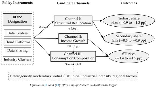
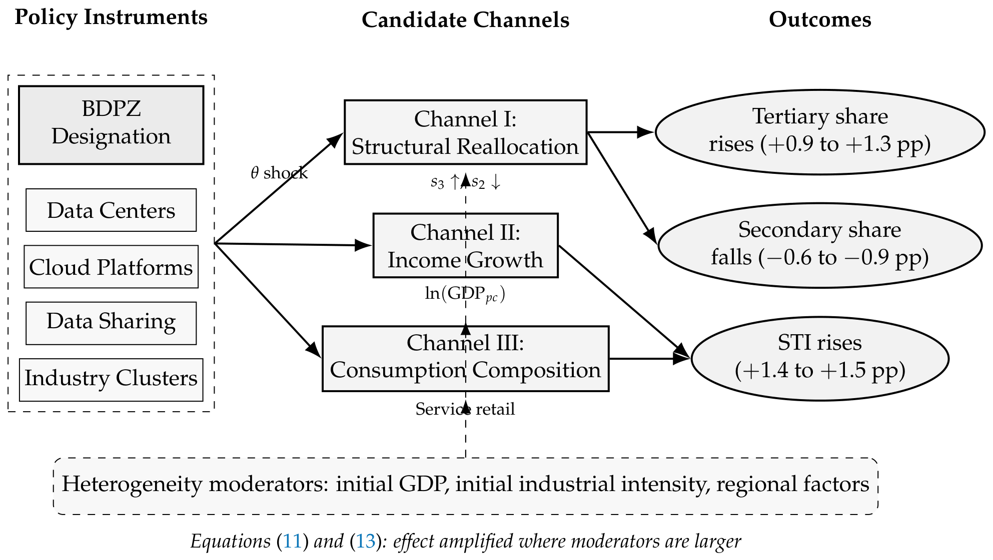
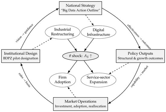
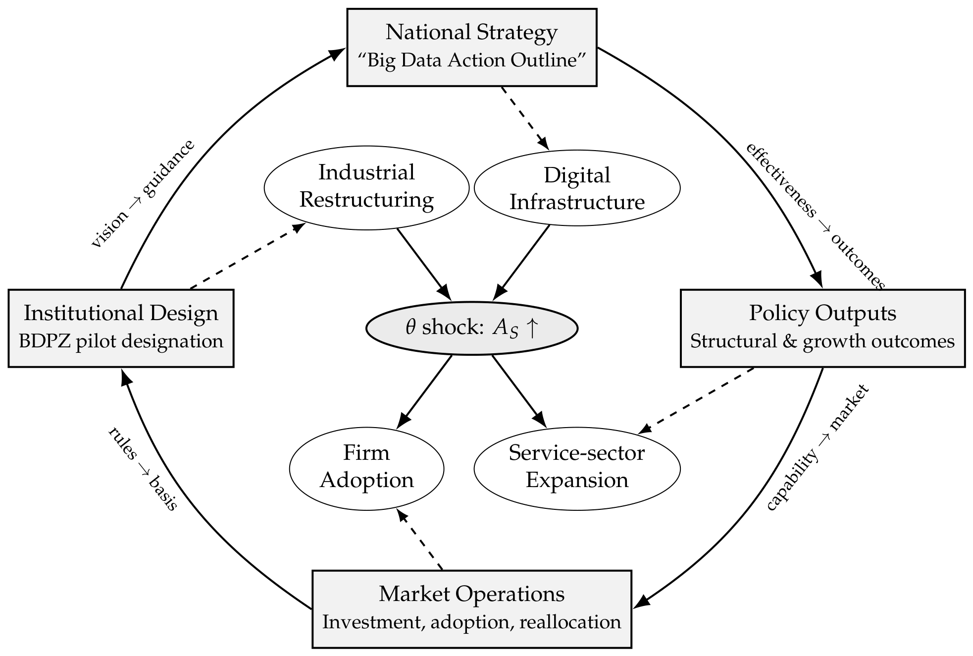
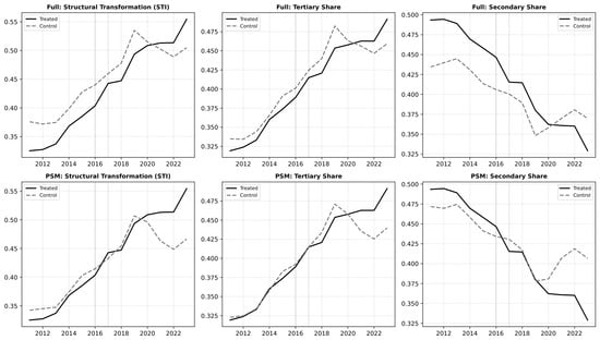
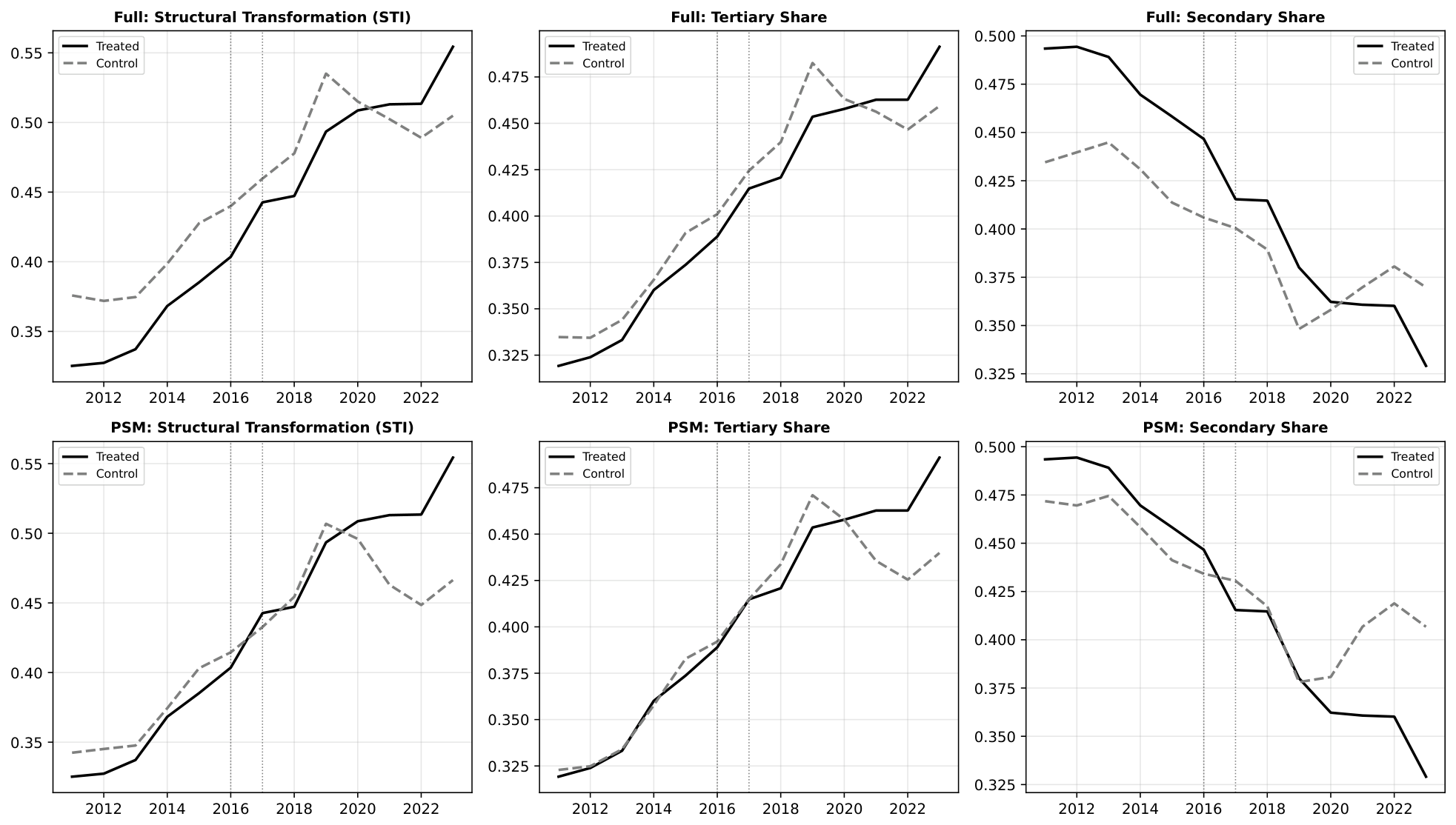
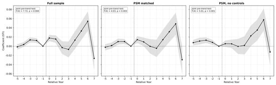
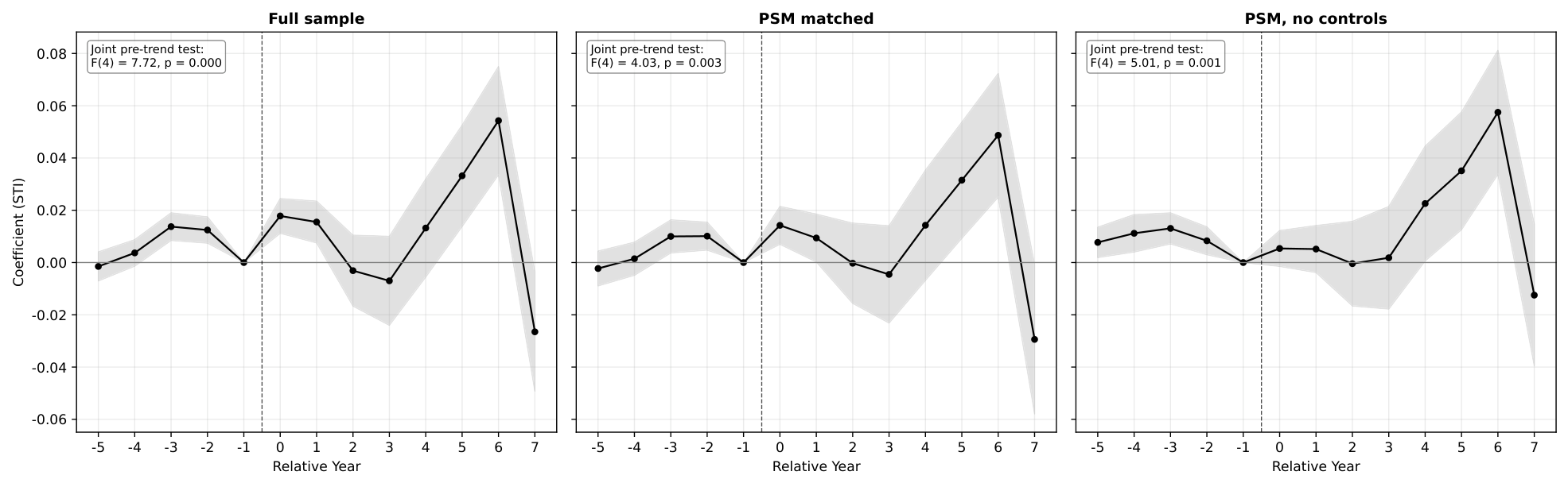
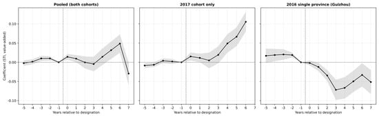
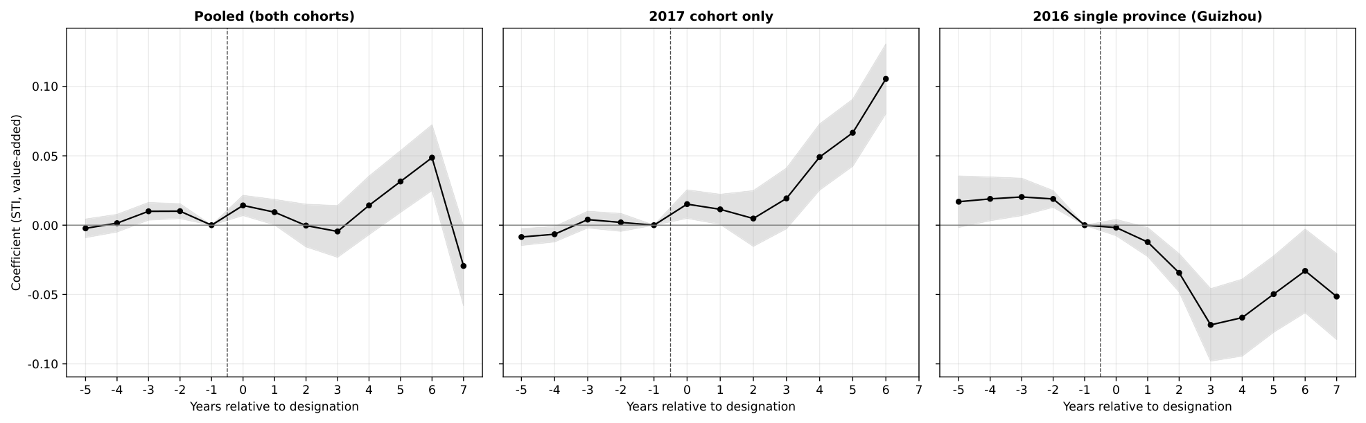
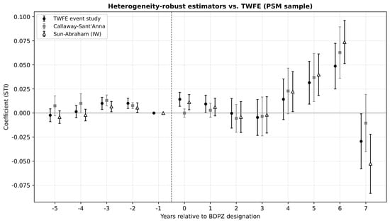
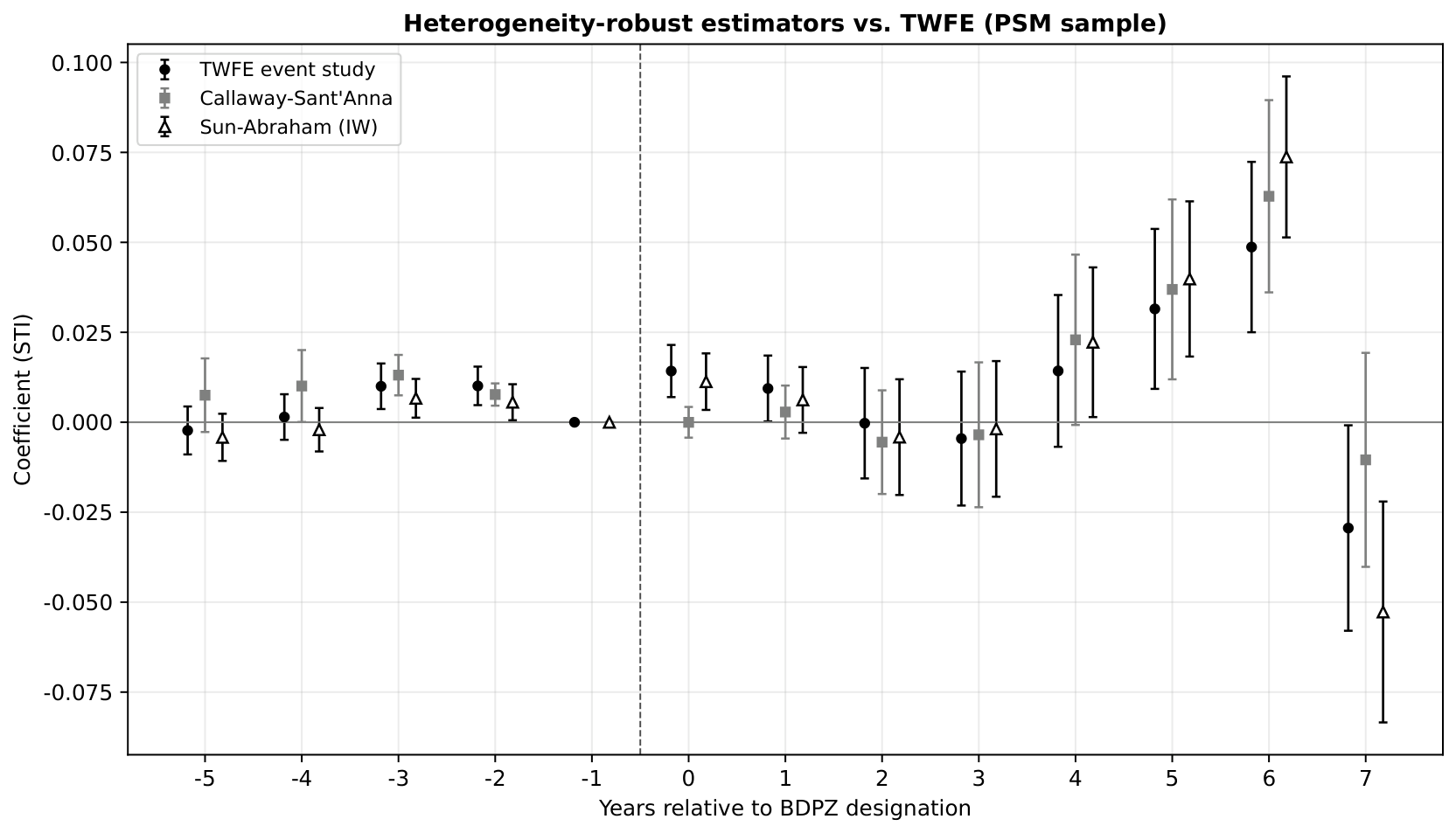
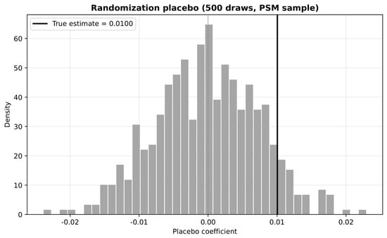
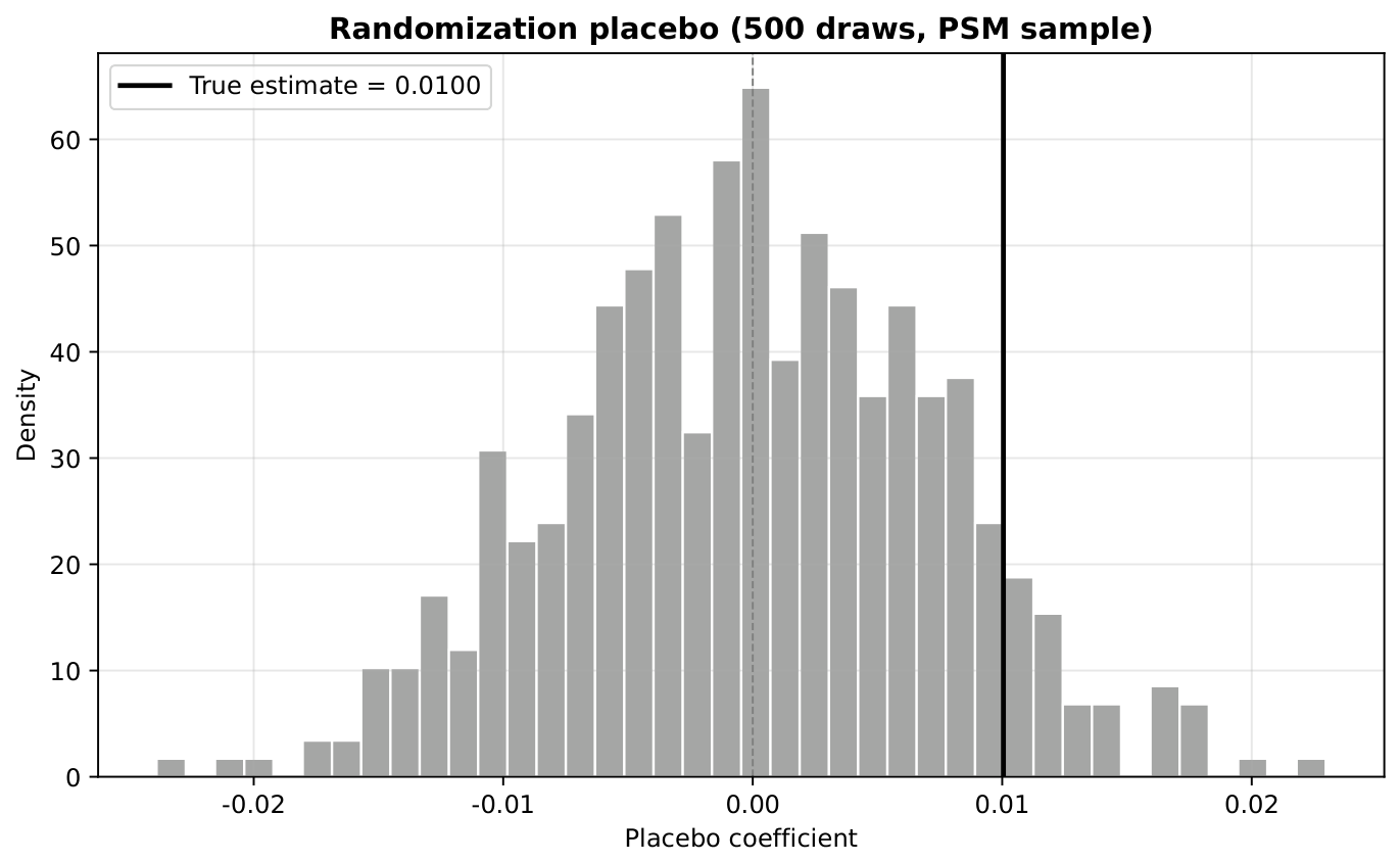

Disclaimer/Publisher’s Note: The statements, opinions and data contained in all publications are solely those of the individual author(s) and contributor(s) and not of MDPI and/or the editor(s). MDPI and/or the editor(s) disclaim responsibility for any injury to people or property resulting from any ideas, methods, instructions or products referred to in the content. |
© 2026 by the authors. Licensee MDPI, Basel, Switzerland. This article is an open access article distributed under the terms and conditions of the Creative Commons Attribution (CC BY) license.