Operating-State-Aware Hydropower Dynamic Support Index and Hierarchical Coordinated Voltage Control for Renewable-Rich Active Distribution Networks

Abstract

With increasing renewable penetration, heterogeneous hydropower resources in active distribution networks exhibit distinct dynamic voltage support characteristics, which makes capacity-based or fixed-weight indices insufficient for state-dependent assessment. This paper proposes an operating-state-aware hydropower dynamic support index (HDSI) and an HDSI-guided hierarchical voltage-control strategy. Conventional synchronous hydropower, variable-speed hydropower, and pumped storage units in synchronous condenser mode are uniformly characterized by a dynamic reactive power margin, response capability, and spatial support efficiency. State-dependent weights are continuously blended according to critical bus voltage deficits and their evolution, and the resulting HDSI is embedded into supervisory reactive power coordination. On a modified IEEE 33-bus system, the proposed HDSI achieves a Spearman correlation of 0.680 with actual dynamic support contribution, compared with 0.655 for the fixed-weight HDSI, with a statistically significant improvement. Under the representative main fault, the proposed control reduces voltage recovery time from 0.344 to 0.172 s and decreases hydropower saturation exposure by 12.9% relative to the fixed-weight method while maintaining comparable voltage recovery. Across 48 structured and 60 randomized scenarios, the control success rate reaches 100%, with a maximum online QP solution time of 12.440 ms. These results demonstrate effective state-aware support assessment and coordinated resource utilization.

1. Introduction

The increasing penetration of distributed photovoltaic and wind generation is transforming conventional radial distribution networks into active distribution networks (ADNs) characterized by multiple generation sources, bidirectional power flows, and increased operational variability. Although renewable generation facilitates distribution-level decarbonization, its intermittency and extensive use of power electronic interfaces substantially alter voltage regulation characteristics. Under operating conditions involving high renewable output, electrically weak feeder sections, and limited local reactive power reserves, rapid power variations and short-circuit disturbances may cause severe voltage violations and delayed post-fault voltage recovery. Multi-timescale Volt/VAR control, coordinated utilization of distributed renewable generation and energy storage, and feedback/data-driven voltage regulation have therefore attracted considerable attention. Zhang et al. developed a double-layer stochastic model predictive voltage-control scheme to coordinate mechanical regulating devices and distributed generation at different timescales [1]. Cao et al. proposed a surrogate-model-assisted deep reinforcement learning approach for fast model-free voltage control [2], whereas Gao and Yu incorporated operational constraints into safe reinforcement-learning-based Volt/VAR control [3]. Pippi et al. coordinated distributed renewable generation and battery storage to address voltage and congestion problems in active distribution grids [4]. These studies demonstrate the growing importance of exploiting flexible resources within ADNs for enhanced voltage security.

As the number of controllable resources increases, voltage regulation has evolved from individual local control toward multi-resource, hierarchical, and distributed coordination. Zhang et al. incorporated smart PV inverters, reactive power devices, and network reconfiguration into Volt/VAR optimization [5]. Meng et al. constructed an electrical-distance metric using voltage sensitivities and coordinated PV units and conventional voltage-control devices through network partitioning and distributed optimization [6]. Jiao et al. developed a real-time distributed voltage-control scheme for coupled medium- and low-voltage distribution networks [7], while Zhang et al. combined system-wide central optimization with fast local inverter control [8]. More recently, Cheng et al. coordinated PV inverters, energy storage, SVGs, and synchronous condensers within a double-layer multi-resource framework [9]. Although these approaches considerably improve the utilization of distributed reactive power resources, their control resources remain dominated by renewable inverters, storage systems, and conventional reactive compensation devices. Comparatively limited attention has been given to the dynamic support-value differences among heterogeneous hydropower resources during disturbances.

Hydropower resources exhibit dynamic characteristics that differ fundamentally from conventional converter-based reactive power devices, while substantial heterogeneity also exists among hydropower technologies. Conventional synchronous hydropower can provide sustained reactive power and voltage support through the synchronous generator and excitation system. Variable-speed hydropower and pumped storage units introduce additional control flexibility through power electronic interfaces, and their dynamic capabilities depend on the active power operating point, converter rating, and control mode. Previous studies have shown that the flexibility of variable-speed pumped storage units varies with operating conditions and active constraints [10]. Full-size-converter-interfaced hydropower plants can exploit rapid converter power regulation to provide dynamic grid support [11], and recent fault ride-through studies have further demonstrated that coordinated rotor- and grid-side converter control can release reactive current capability to enhance voltage support during severe voltage sags [12]. Synchronous condensers are also increasingly employed in renewable-rich grids because of their short-circuit strength, dynamic reactive power, and synchronous-machine characteristics; however, their dynamic performance depends strongly on operating condition, electrical location, and excitation control [13,14]. These findings indicate that the support priority of hydropower and synchronous-machine-based resources cannot be prescribed solely according to resource type.

From a methodological perspective, the most pertinent studies address different aspects of dynamic voltage support. Meng et al. [6] employed voltage-sensitivity-based electrical distance for network partitioning, whereas Cheng et al. [9] combined power sensitivity and reserve information for multi-resource coordination. Zhang et al. [8] coordinated system-wide optimization and fast local inverter control, while Xu et al. [10] evaluated the operating-point-dependent flexibility of variable-speed pumped storage for frequency regulation. Although these methods account for electrical location, available regulation capacity, or different control timescales, they do not jointly quantify the available reactive power margin, deliverable response speed, and critical bus voltage support effectiveness within a calibrated, disturbance-state-dependent resource-value index. By contrast, the proposed HDSI combines these three normalized attributes and identifies their relative importance against actual dynamic support contribution (ADSC) under representative operating states. The calibrated weights are subsequently blended according to the voltage deficit and its temporal evolution, which enables resource-value assessment to adapt continuously across mild regulation, voltage arrest, and post-fault recovery.

Beyond resource assessment, the main methodological distinction lies in how the evaluated support value influences closed-loop decisions. Existing hierarchical approaches [1,7,8,9] coordinate local response with supervisory optimization but do not explicitly incorporate an ADSC-calibrated hydropower support index into resource allocation costs. In the proposed strategy, the updated HDSI is mapped to resource-specific reactive power regulation costs within the supervisory quadratic program, which allows the relative allocation priorities to change with the operating state while satisfying network voltage and device capability constraints. Meanwhile, local excitation and converter controllers provide immediate voltage support, and supervisory coordination adjusts subsequent reactive power references. Therefore, the contribution lies in coupling calibrated multidimensional support assessment with state-dependent allocation and hierarchical closed-loop control rather than introducing hierarchical coordination alone.

To address these issues, this paper proposes an operating-state-aware hydropower dynamic support index (HDSI) and an HDSI-guided hierarchical coordinated voltage-control strategy for renewable-rich ADNs. Rather than prescribing a fixed priority for a particular hydropower technology, the proposed framework evaluates the dynamic resource value according to current device capability, network electrical coupling, and voltage disturbance state and directly incorporates this value into supervisory reactive power allocation. The main contributions are summarized as follows.

(1) A unified dynamic voltage support capability representation is developed for heterogeneous hydropower resources. The distinct characteristics of CSH, VSH, and PSC resources are mapped onto three physically interpretable dimensions: dynamic reactive power margin M_Q, dynamic response capability R_Q, and spatial voltage support efficiency E. These dimensions respectively quantify how much support is available, how fast it can be delivered, and how effectively it influences critical buses, enabling consistent comparison across heterogeneous technologies.

(2) An operating-state-aware HDSI is proposed. The weighted critical bus voltage deficit and its temporal evolution are used to continuously characterize the mild-regulation, voltage-arrest, and voltage recovery states. Archetypal weighting factors are identified offline against the actual dynamic support contribution (ADSC) under representative scenarios and continuously blended online through state memberships. The resulting HDSI therefore avoids manually prescribed fixed weights and adapts to disturbance severity, recovery stage, and current resource capability.

(3) An HDSI-guided hierarchical coordinated voltage-control strategy is established. A fast local support–supervisory coordination architecture is adopted, and the HDSI is directly mapped into the marginal reactive power regulation cost of hydropower resources rather than being used only for static ranking. Consequently, hydropower resources and renewable inverters are continuously coordinated according to their dynamic support values while satisfying voltage and device capability constraints. Independent validation, ablation, multidisturbance, and communication-delay studies are further performed to assess ranking fidelity, closed-loop effectiveness, robustness, and real-time feasibility.

2. Dynamic Voltage Support Modeling of Hydropower-Integrated Active Distribution Networks

2.1. System Configuration and Voltage Support Mechanism

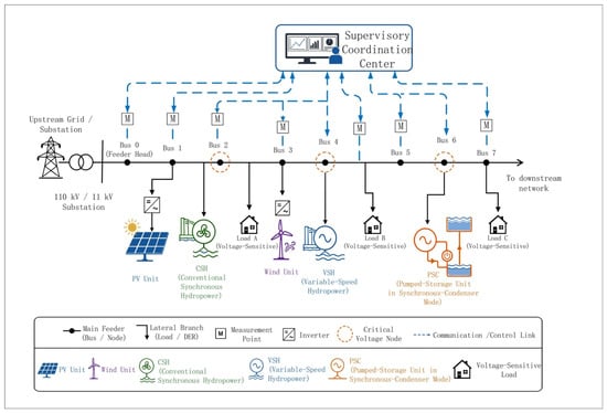
Consider a renewable-rich active distribution network (ADN) incorporating distributed renewable generation and heterogeneous hydropower resources, as illustrated in Figure 1. The system consists of an upstream grid, distribution feeders, distributed photovoltaic and wind generation, voltage-sensitive loads, and multiple types of hydropower resources. The hydropower resources considered in this study include conventional synchronous hydropower (CSH), variable-speed hydropower (VSH), and pumped storage units operating in synchronous condenser mode (PSC). These resources are connected to different buses through their respective grid interfaces and jointly participate in dynamic voltage support following disturbances [15,16,17].

Figure 1. Configuration of a renewable-rich active distribution network with heterogeneous hy-dropower resources.

Let the sets of network buses, hydropower resources, renewable resources, and critical voltage buses be denoted by Ω_N, Ω_H, Ω_R, Ω_C ⊆ Ω_N, respectively. The set Ω_C may include feeder-end buses, renewable-rich buses, critical-load buses, and historically weak-voltage buses.

Following renewable power fluctuations, load variations, or short-circuit disturbances, bus voltage variations depend not only on the overall reactive power balance but also on the electrical locations of available support resources. Linearizing the AC power-flow equations around the current operating point gives

$$\left[\begin{array}{c}\Delta P\\ \Delta Q\end{array}\right]=\left[\begin{array}{cc}{J}_{\mathit{P\theta }}& J_{\mathit{PV}}\\ J_{\mathit{Q\theta }}& J_{\mathit{QV}}\end{array}\right]\left[\begin{array}{c}\Delta \theta \\ \Delta V\end{array}\right].$$

(1)

Here, ΔP and ΔQ denote the incremental active and reactive power injections, respectively; Δθ and ΔV are the corresponding variations in voltage angles and magnitudes; and J_Pθ, J_PV, J_Qθ, and J_QV are submatrices of the power-flow Jacobian evaluated at the current operating point.

By eliminating the voltage-angle increment, the reduced voltage–reactive power relationship can be written as

$$\Delta V=S_{\mathit{VQ}}\Delta Q{S}_{\mathit{VQ}}={\left(J_{\mathit{QV}}-J_{\mathit{Q\theta }}{J}_{\mathit{P\theta }}^{-1}{J}_{\mathit{PV}}\right)}^{-1},$$

(2)

where S_VQ is the reduced voltage–reactive power sensitivity matrix. Its element S_VQ,ih characterizes the local influence of a unit reactive power variation at the connection bus of hydropower resource h on the voltage magnitude of critical bus i.

Equation (2) indicates that resources providing the same amount of reactive power may produce significantly different voltage support effects because of their different electrical locations. Therefore, the dynamic voltage support capability of a hydropower resource should not be determined solely by its rated capacity. Its available reactive power capability, dynamic response speed, and spatial effectiveness with respect to critical buses must be jointly considered.

2.2. Dynamic Support Models of Heterogeneous Hydropower Resources

Different hydropower resources exhibit distinct grid-interface configurations and reactive power regulation mechanisms. For the dynamic voltage support and supervisory coordination problem considered in this paper, high-order models containing all mechanical and electromagnetic states are unnecessary. Instead, the dominant external characteristics and operational constraints that directly determine reactive power support capability should be retained. Accordingly, dynamic reactive power boundaries and equivalent response models are adopted to characterize the three resource types [18,19].

2.2.1. Conventional Synchronous Hydropower

A CSH unit regulates its terminal voltage primarily through the excitation system of the synchronous generator. Its reactive power capability is jointly constrained by the excitation limit, stator-current capability, and current operating point. At the supervisory coordination level,

$$Q_h^{\mathit{min}}(t)\le Q_h(t)\le Q_h^{\mathit{max}}(t),\hspace{1em}h\in {\mathrm{\Omega }}_{\mathit{CSH}}.$$

(3)

The external reactive power response under excitation regulation is represented by

$$T_{Q,h}^{\mathit{CSH}}{\displaystyle \frac{d{Q}_h(t)}{\mathit{dt}}}+Q_h(t)=Q_h^{\mathit{ref}}(t),$$

(4)

Subject to

$$\left|{\displaystyle \frac{d{Q}_h(t)}{\mathit{dt}}}\right|\le R_{Q,h}^{\mathit{max}}.$$

(5)

Here, $T_{Q,h}^{\mathit{CSH}}$ is the equivalent reactive power response time constant, $Q_h^{\mathit{ref}}$ is the reactive power reference, and $R_{Q,h}^{\mathit{max}}$ denotes the maximum allowable reactive power ramp rate.

CSH units are characterized by relatively large sustained reactive power capability and inherent synchronous-machine voltage support. Their fast reactive power regulation, however, is constrained by excitation system dynamics and machine operating limits. They are therefore particularly suitable for sustained postdisturbance voltage support.

2.2.2. Variable-Speed Hydropower

For a converter-interfaced VSH unit under voltage-oriented control, the (q)-axis voltage component can be approximately set to zero. The active and reactive power outputs are then expressed as

$$\begin{array}{l}{P}_h={\displaystyle \frac{3}{2}}{u}_{d,h}{i}_{d,h},\hspace{1em}\\ Q_h=-{\displaystyle \frac{3}{2}}{u}_{d,h}{i}_{q,h}\end{array},$$

(6)

where u_d,h denotes the d-axis voltage at the point of common coupling (PCC) and i_d,h and i_q,h represent the d- and q-axis currents of the converter, respectively.

Considering the converter-current limit,

$$i_{d,h}^2+i_{q,h}^2\le {\left(I_h^{\mathit{max}}\right)}^2.$$

(7)

Combining (6) and (7), the reactive power capability at a given active power operating point is bounded by

$$\left|Q_h(t)\right|\le \sqrt{{\left({\displaystyle \frac{3}{2}}{u}_{d,h}(t)I_h^{\mathit{max}}\right)}^2-P_h^2(t)}.$$

(8)

Equation (8) describes the theoretical voltage-dependent converter-current capability of a VSH unit, which requires the active power operating point to remain within the corresponding current limit. In the present controller-level implementation, the reactive power headroom is approximated using the nominal apparent power rating and prescribed active power, with a nonnegative radicand imposed numerically. When the prescribed active power exceeds the nominal capability, the calculated reactive power headroom is set to zero. However, this numerical treatment does not represent active power curtailment or guarantee current feasibility during severe voltage sags. Within the adopted simplified model, VSH units retain their fast reactive power regulation characteristics and can provide rapid voltage support through converter control.

2.2.3. Pumped Storage in Synchronous Condenser Mode

When a pumped storage unit operates in synchronous condenser mode, active power exchange is small, while the synchronous machine and excitation system can be mainly utilized for reactive power regulation. Its external reactive power response at the supervisory coordination timescale is represented by [20,21]

$$T_{Q,h}^{\mathit{PSC}}{\displaystyle \frac{d{Q}_h(t)}{\mathit{dt}}}+Q_h(t)=Q_h^0+K_{V,h}\left[V_h^{\mathit{ref}}-V_h(t)\right],$$

(9)

Subject to

$$Q_h^{\mathit{min}}\le Q_h(t)\le Q_h^{\mathit{max}},\hspace{1em}h\in {\mathrm{\Omega }}_{\mathit{PSC}}.$$

(10)

Here, $Q_h^0$ denotes the initial reactive power operating point, K_V,h is the equivalent voltage–reactive power regulation gain, $V_h^{\mathit{ref}}$ is the voltage reference, and $T_{Q,h}^{\mathit{PSC}}$ is the equivalent reactive power response time constant.

Because a unit operating in synchronous-condenser mode transfers little active power, a larger proportion of its capability can be utilized for reactive power regulation. PSC units therefore typically possess substantial dynamic reactive power reserve and are well suited to strong and sustained voltage support near critical weak-voltage buses. The main dynamic voltage-support characteristics, response features, and operating constraints of the three hydropower resource types are summarized in Table 1.

Table 1. Dynamic voltage support characteristics of heterogeneous hydropower resources.

Resource	Main Mechanism	Reactive Power Characteristic	Response	Dominant Constraint
CSH	Excitation regulation	Large sustained support	Moderate	Excitation and machine limits
VSH	Converter reactive-current control	Operating-point-dependent	Fast	Converter-current limit
PSC	Excitation-based synchronous condenser support	Large reactive reserve	Fast and sustained	Excitation and machine capability

Table 1. Dynamic voltage support characteristics of heterogeneous hydropower resources.

Resource	Main Mechanism	Reactive Power Characteristic	Response	Dominant Constraint
CSH	Excitation regulation	Large sustained support	Moderate	Excitation and machine limits
VSH	Converter reactive-current control	Operating-point-dependent	Fast	Converter-current limit
PSC	Excitation-based synchronous condenser support	Large reactive reserve	Fast and sustained	Excitation and machine capability

Overall, CSH, VSH, and PSC do not exhibit a universally fixed support priority. The dynamic support value of an individual resource depends not only on its resource type but also on its current active–reactive operating point, available reactive reserve, response speed, and electrical coupling with the controlled buses. A unified dynamic support representation applicable across heterogeneous resource types is therefore required.

2.3. Unified Representation of Dynamic Voltage Support Capability

To enable a unified, quantitative comparison of heterogeneous hydropower resources, this paper—starting from the requirements for dynamic voltage support—decomposes the support capability of resource h at time t into three mutually independent dimensions, each with a clear physical meaning:

$${\mathcal{C}}_h(t)={\left[M_{Q,h}(t),R_{Q,h}(t),E_h(t)\right]}^T.$$

(11)

Here, M_Q,h denotes the dynamic reactive power margin and characterizes how much additional reactive power can be provided, R_Q,h represents the dynamic response capability and characterizes how fast the available reactive power can be delivered, and E_h represents the spatial voltage support efficiency and characterizes how effectively the reactive power injection influences critical buses.

Accordingly, the dynamic voltage support capability of heterogeneous hydropower resources can be interpreted through three fundamental dimensions:

2.3.1. Dynamic Reactive Power Margin

For low-voltage support, an available resource generally improves bus voltage by increasing positive reactive power injection. The currently available reactive power of resource (h) is therefore defined as

$$Q_h^{\mathit{ava}}(t)=Q_h^{\mathit{max}}(t)-Q_h(t).$$

(12)

The corresponding dynamic reactive power margin is normalized over the full feasible reactive power range to account for both reactive power injection and absorption:

$$M_{Q,h}(t)={\mathrm{sat}}_{[0,1]}\left({\displaystyle \frac{Q_h^{\mathit{ava}}(t)}{\max \left\{Q_h^{\mathit{max}}(t)-Q_h^{\mathit{min}}(t),{\epsilon }_Q\right\}}}\right),$$

(13)

where $Q_h^{\min }(t)$ and $Q_h^{\max }(t)$ denote the feasible reactive power limits, ε_Q > 0is a small constant for numerical protection, and sat_[0,1](⋅) bounds the indicator within [0, 1]. The proposed normalization accounts for the full feasible reactive power range, including reactive power absorption. Consequently, 0 ≤ M_Q,h(t) ≤ 1 holds throughout the feasible operating envelope, with a larger value indicating a greater fraction of available upward reactive power regulation capability.

2.3.2. Dynamic Response Capability

A large reactive power reserve alone does not guarantee effective dynamic voltage support. During the short postdisturbance voltage recovery interval, the resource must also be capable of releasing its available reactive power sufficiently rapidly. The dynamic response capability is therefore defined as

$$R_{Q,h}={\displaystyle \frac{\Delta Q_h^{\mathit{fast}}}{T_h^{\mathit{resp}}{Q}_h^{\mathit{rated}}}}.$$

(14)

Here, $\Delta Q_h^{\mathit{fast}}$ denotes the reactive power increment that can be delivered within a specified fast support time window, $T_h^{\mathit{resp}}$ is the corresponding response time, and $Q_h^{\mathit{rated}}$ denotes the rated reactive power capability.

Compared with response time alone, Equation (14) considers both response speed and the magnitude of deliverable reactive power.

2.3.3. Spatial Voltage Support Efficiency

The effectiveness of reactive power support also depends on the electrical location of the resource. Based on the voltage–reactive power sensitivity matrix in (2), the spatial support efficiency of hydropower resource (h) with respect to the critical bus set is defined as

$$\begin{array}{l}{E}_h(t)={\displaystyle \sum _{i\in {\mathrm{\Omega }}_C}{\alpha }_i}\left|S_{\mathit{VQ},\mathit{ih}}(t)\right|\\ {\displaystyle \sum _{i\in {\mathrm{\Omega }}_C}{\alpha }_i.}=1,\hspace{1em}{\alpha }_i\ge 0\end{array}.$$

(15)

Here, α_i is the importance weight assigned to critical bus i. A resource electrically close to feeder-end weak buses, renewable-rich buses, or critical-load buses generally exhibits a larger value of E_h.

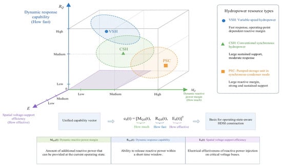
It should be emphasized that M_Q,h, R_Q,h, and E_h describe the capacity, temporal, and spatial characteristics of a resource, respectively. Treating these characteristics as separate evaluation dimensions avoids conflating reactive power availability, response speed, and electrical location within a single parameter. This multidimensional representation therefore establishes a physically interpretable basis for the composite dynamic support index developed in the following section. A three-dimensional representation of dynamic voltage support capability is introduced in Figure 2.

Figure 2. Unified representation of dynamic voltage support capability for heterogeneous hydropower resources.

As illustrated in Figure 2, the proposed capability space decomposes the dynamic voltage support performance of each hydropower resource into three orthogonal and physically meaningful dimensions, namely, the reactive power margin M_Q,h, the response capability R_Q,h, and the spatial effectiveness E_h. This representation clearly reveals that heterogeneous hydropower units may exhibit similar performance in one dimension while differing significantly in others, thereby highlighting the necessity of a multidimensional evaluation framework rather than a single capacity-based metric. In particular, the figure emphasizes that the overall support capability is jointly determined by “how much reactive power can be provided”, “how fast it can be delivered”, and “how effectively it influences critical voltage-sensitive buses”, which directly motivates the development of the HDSI in the following section.

3. Operating-State-Aware Hydropower Dynamic Support Index

3.1. Normalized Dynamic Support Capability and Operating-State Characterization

Because the dynamic reactive power margin M_Q,h, dynamic response capability R_Q,h, and spatial voltage support efficiency E_h have different physical meanings and numerical scales, they must be normalized before constructing the composite index. To avoid nonphysical changes in the normalized values when resources enter or leave the available resource set, fixed reference bounds derived from equipment operating envelopes and representative offline scenarios are adopted rather than instantaneous extrema. For an arbitrary indicator x_j,h(t), where j ∈ M,R,E:

$${\overline{x}}_{j,h}(t)=\mathrm{sat}\left[{\displaystyle \frac{x_{j,h}(t)-x_j^{\mathit{min}}}{x_j^{\mathit{max}}-x_j^{\mathit{min}}+\epsilon }},0,1\right],$$

(16)

where sat[x,0,1] limits (x) to the interval [0,1]; $x_j^{\mathit{min}}$ and $x_j^{\mathit{max}}$ are the reference lower and upper bounds over the predefined operating envelope, respectively; and ε is a small positive constant.

With the full-range normalization and explicit bounding introduced in Equation (13), the reactive power margin satisfies 0 ≤ M_Q,h(t) ≤ 1 throughout the feasible operating envelope, including reactive power absorption. Therefore, ${\overline{M}}_{Q,h}(t)=M_{Q,h}(t)$ can be directly used without further normalization. The response capability and spatial effectiveness are normalized using Equation (16), which ensures that all three components of the capability vector lie within [0,1].

$${\overline{\mathcal{C}}}_h(t)={\left[{\overline{M}}_{Q,h}(t),{\overline{R}}_{Q,h}(t),{\overline{E}}_h(t)\right]}^T,$$

(17)

The normalized dynamic support capability vector of resource h is given by Equation (17), which maps the three physical characteristics onto a common [0,1] scale.

Equation (17) maps the three physical characteristics onto a common [0,1] scale, thereby providing a consistent numerical basis for cross-resource comparison and composite assessment.

In addition to the resource capability itself, the HDSI should reflect the current system demand for dynamic voltage support. Let $V_i^{\mathit{ref}}$ denote the reference voltage of critical bus i. The weighted voltage-deficit index is defined as

$$\begin{array}{l}{D}_V(t)={\displaystyle \sum _{i\in {\mathrm{\Omega }}_C}{\alpha }_i}{\displaystyle \frac{{\left[V_i^{\mathit{ref}}-V_i(t)\right]}_{+}}{V_i^{\mathit{ref}}}}\\ {[x]}_{+}=\max (x,0)\end{array}.$$

(18)

The index D_V(t) accounts for both the voltage deviation and the relative importance of multiple critical buses. It approaches zero when the critical bus voltages remain close to their reference values and increases as the voltage depression becomes more severe.

The normalized voltage disturbance severity is then defined as

$${\delta }_V(t)=\min \left[1,{\displaystyle \frac{D_V(t)}{D_V^{\mathit{sat}}}}\right],$$

(19)

where $D_V^{\mathit{sat}}$ denotes the saturation level determined according to the allowable voltage deviation and representative offline disturbance scenarios.

The voltage-deficit magnitude alone cannot distinguish whether the voltage condition is deteriorating or recovering. Therefore, the temporal derivative ${\dot{D}}_V(t)$ is further introduced, and three continuous state-membership coefficients are defined as

$$\begin{array}{l}{\mu }_M(t)=1-{\delta }_V(t)\\ {\mu }_A(t)={\displaystyle \frac{{\delta }_V(t)}{2}}\left[1+\tanh \left(\kappa {\dot{D}}_V(t)\right)\right]\\ {\mu }_R(t)={\displaystyle \frac{{\delta }_V(t)}{2}}\left[1-\tanh \left(\kappa {\dot{D}}_V(t)\right)\right]\\ {\mu }_M(t)+{\mu }_A(t)+{\mu }_R(t)=1\end{array}.$$

(20)

Here, μ_M, μ_A, and μ_R denote the memberships of the mild-regulation state, voltage-arrest state, and voltage recovery state, respectively, and κ > 0 controls the smoothness of the state transition.

When the voltage deviation is small, δ_V is low and the mild-regulation state dominates. During a severe voltage sag, if D_V continues to increase, i.e., ${\dot{D}}_V>0$, the voltage-arrest membership increases, which indicates an urgent requirement to prevent further voltage deterioration. After fault clearance, when D_V begins to decrease, i.e., ${\dot{D}}_V<0$, the voltage recovery membership gradually becomes dominant. Compared with hard threshold-based switching, (20) provides a continuous transition among different voltage support stages and prevents abrupt changes in the HDSI weighting factors.

3.2. Operating-State-Aware HDSI Formulation

The essential feature of the proposed HDSI is not simply the replacement of one set of fixed weights with another but also the establishment of a data-supported mapping between the system operating state and the relative importance of different support dimensions. To reduce the subjectivity associated with manually selected weighting factors, representative offline scenarios are first employed to identify archetypal weight vectors for the mild-regulation, voltage-arrest, and voltage recovery states. These state-dependent weights are subsequently blended online using the continuous memberships defined in (20).

Let ${\omega }_Q^s,{\omega }_R^s,{\omega }_E^s$ denote the archetypal HDSI weight vector associated with state s. For the offline scenario set $𝒟$_s, the state-dependent weights are obtained by solving

$$\begin{array}{l}{\min }_{{\omega }^s}{\displaystyle \frac{1}{\left|{\mathcal{P}}_s\right|}}{\displaystyle \sum _{(k,i,j)\in {\mathcal{P}}_s}\ln }\left[1+\exp \left(-\beta {\sigma }_{\mathit{kij},s}{({\omega }^s)}^{\mathrm{T}}\Delta {\overline{\mathcal{C}}}_{\mathit{kij},s}\right)\right]+{\lambda }_{\omega }\Vert {\omega }^s-{\omega }^0{\Vert }_2^2\\ {\mathbf{1}}^T{\omega }^s=1,\hspace{1em}{\omega }^s\ge \mathbf{0}\\ \Delta {\overline{\mathcal{C}}}_{\mathit{kij},s}={\overline{\mathcal{C}}}_{i,k,s}-{\overline{\mathcal{C}}}_{j,k,s}\\ {\sigma }_{\mathit{kij},s}=\mathrm{sign}({\overline{\mathrm{\Gamma }}}_{i,k,s}-{\overline{\mathrm{\Gamma }}}_{j,k,s})\end{array}.$$

(21)

Here, $𝒫$_s denotes the valid resource-pair set for operating state s, $\Delta {\overline{\mathcal{C}}}_{\mathit{kij},s}$ is the difference between the normalized capability vectors of resources i and j, and σ_kij,s denotes the sign of their ADSC difference. Pairs with an ADSC difference below 10⁻⁸ are excluded. The pairwise logistic ranking loss is adopted to align weight calibration with the resource-ranking objective. The ranking parameter and regularization coefficient are set to β = 10 and λ_ω = 0.05, respectively, with ω⁰ = [1/3,1/3,1/3]^T. The constrained problem is solved using the interior-point algorithm.

The constraints 1^Tω^s = 1 and ω^s ≥ 0 preserve the convex-combination interpretation of the three support dimensions. Unlike manually specified fixed weighting factors, the formulation in (21) identifies the relative importance of the three dimensions from their consistency with actual voltage support contribution while maintaining physical interpretability.

During online operation, the three state-membership coefficients calculated from (20) are used to continuously blend the offline archetypal weights:

ω(t) = μ_M(t)ω^M + μ_A(t)ω^A + μ_R(t)ω^R.

(22)

Because the state memberships sum to unity, the resulting weights automatically satisfy ω_Q(t) + ω_R(t) + ω_E(t) = 1,  ω_Q(t),ω_R(t),ω_E(t) ≥ 0. No online weight optimization is therefore required. Only the voltage-state memberships and a linear combination of the pre-identified weight vectors need to be updated, which keeps the real-time computational burden low. The operating-state-aware HDSI of resource h is finally defined as

$$\mathit{HDS}{I}_h(t)={\omega }_Q(t){\overline{M}}_{Q,h}(t)+{\omega }_R(t){\overline{R}}_{Q,h}(t)+{\omega }_E(t){\overline{E}}_h(t).$$

(23)

Because all normalized capability indicators are bounded within [0,1], and the calibrated archetypal weight vectors are nonnegative and sum to unity, the online blended weights also form a convex combination. Consequently, 0 ≤ HDSI_h(t) ≤ 1 holds for every feasible operating point. This bound remains valid when a hydropower resource operates in the reactive power absorption region, which ensures that the index can be consistently used in the subsequent coordinated optimization.

A larger HDSI_h indicates that the resource provides greater dynamic support value under the current system condition and should therefore receive higher priority in the subsequent coordinated voltage-control process.

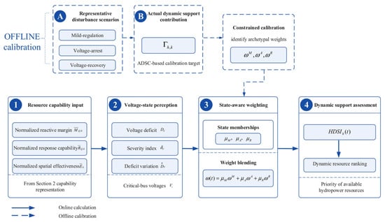
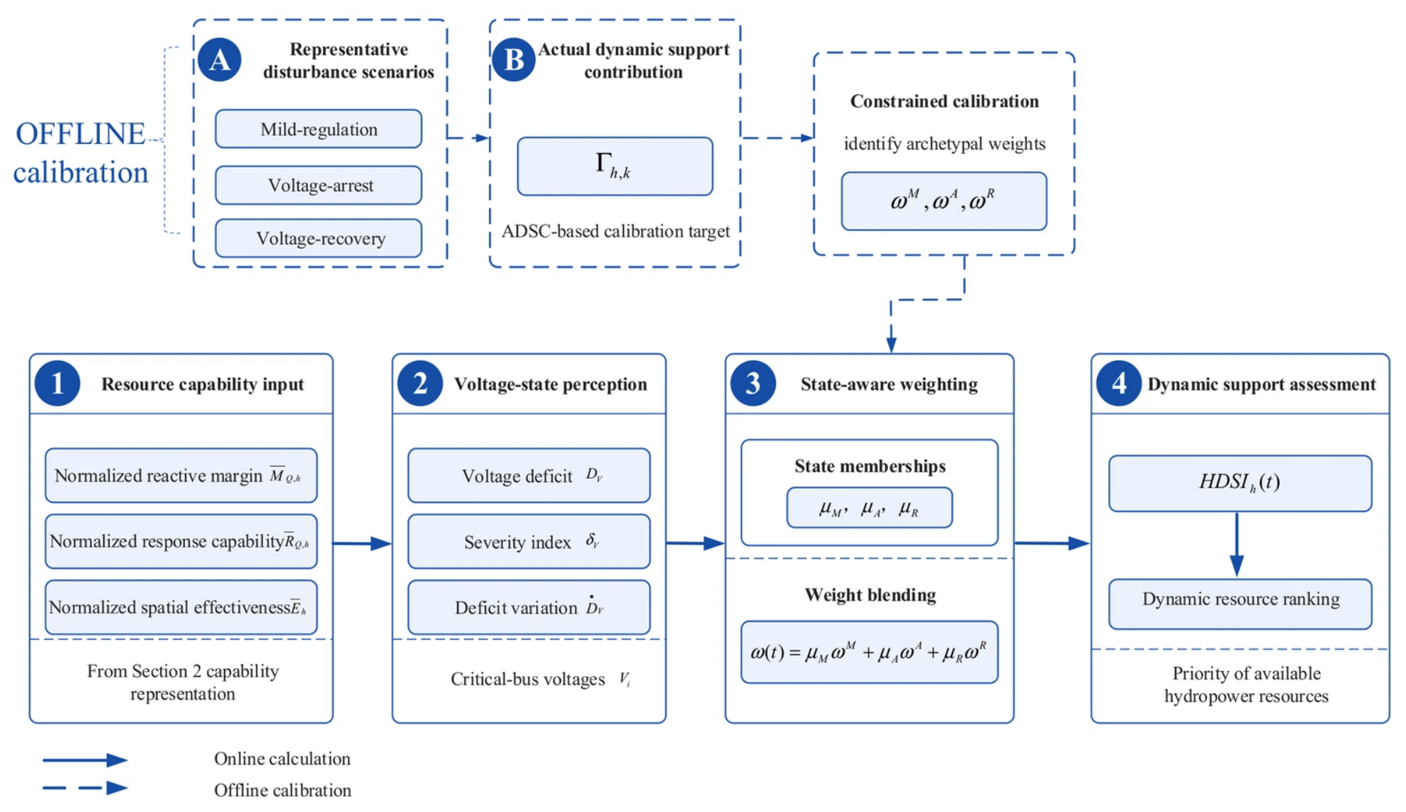
The computational process for operational-state-aware HDSI can be summarized as comprising four steps, as illustrated in Figure 3: input of resource capacity, detection of system voltage status, updating of state-dependent weights, and evaluation of dynamic support capacity.

Figure 3. Construction of the operating-state-aware hydropower dynamic support index.

As shown in Figure 3, the inputs from the resource side include the normalized dynamic reactive power margin, dynamic response capability and spatial voltage support efficiency; the inputs from the system side include voltage shortfalls at key nodes, disturbance severity and its rate of change. During the offline phase, the constrained calibration method is utilized to obtain reference weights for various typical operating states; during the online phase, state membership is calculated based on real-time voltage conditions, and weight fusion and HDSI updates are performed. Ultimately, the resulting HDSI is used to establish a dynamic resource priority ranking for the current operating state.

3.3. HDSI-Based Resource Ranking and Validation Criterion

The purpose of the HDSI is not merely to generate a dimensionless score but also to ensure that this score is consistent with the actual contribution of a resource to postdisturbance voltage recovery. An independent physical benchmark, which does not participate in the HDSI calculation itself, is therefore introduced to evaluate the validity of the resource ranking. For an offline disturbance scenario k, the weighted voltage-deficit integral without dynamic hydropower support is first defined as

$$J_{V,k,s}^0={\displaystyle {\int }_{t_{k,s}^{\mathit{start}}}^{t_{k,s}^{\mathit{end}}}{\displaystyle \sum _{i\in {\mathrm{\Omega }}_C}{\alpha }_i}}{[V_i^{\mathit{ref}}-V_{i,k}^0(t)]}_{+}\mathit{dt},$$

(24)

where $t_{k,s}^{\mathit{start}}$ and $t_{k,s}^{\mathit{end}}$ denote the starting and ending times of the evaluation window for operating state s in disturbance scenario k, respectively, and $V_{i,k}^0(t)$ represents the voltage response of critical bus i in the baseline case without dynamic hydropower support.

Under the same initial operating condition and disturbance, hydropower resource h is then enabled to provide dynamic reactive power support, yielding

$$J_{V,h,k,s}={\displaystyle {\int }_{t_{k,s}^{\mathit{start}}}^{t_{k,s}^{\mathit{end}}}{\displaystyle \sum _{i\in {\mathrm{\Omega }}_C}{\alpha }_i}}{[V_i^{\mathit{ref}}-V_{i,h,k}(t)]}_{+}\mathit{dt}.$$

(25)

The actual dynamic support contribution (ADSC) of resource (h) in scenario (k) is defined as

$${\mathrm{\Gamma }}_{h,k,s}=\max \left\{{\displaystyle \frac{J_{V,k,s}^0-J_{V,h,k,s}}{\max \{J_{V,k,s}^0,{10}^{-8}\}}},0\right\}$$

(26)

Here, s ∈ M,A,R denotes the mild-regulation, voltage-arrest, and voltage recovery states, respectively. The corresponding offline ADSC evaluation windows are [t_{c,k} + 0.65,1.8] s, [t_{c,k},t_{c,k} + 0.05] s, and [t_{c,k} + 0.05,t_{c,k} + 0.65] s, where t_{c,k} is the fault-clearing time of scenario (k). The voltage-arrest window represents the early post-fault response interval in the offline calibration.

For each disturbance scenario, the baseline case without dynamic hydropower support and three single-resource support cases are simulated under identical initial conditions and disturbances. The reactive power margin and response capability are extracted from the last pre-fault capability snapshot, while spatial effectiveness is sampled at 35% of the corresponding state-specific evaluation window. The resulting capability vector is paired with the ADSC calculated from the reduction in the critical bus voltage-deficit integral over the same scenario and state-specific window. Thus, each calibration sample establishes an explicit correspondence between prospective resource capability, state-dependent electrical effectiveness, and the actual support contribution.

A larger Γ_h,k,s indicates a greater contribution of resource h to reducing the voltage deficit during state s of scenario k. The state-specific ADSC targets are normalized using calibration-derived reference bounds before construction of the pairwise ranking samples in Equation (21). The ADSC is used only for offline calibration and independent validation, rather than as an online control input.

For offline calibration, the reactive power margin and response capability are obtained from the final pre-fault capability snapshot, while spatial effectiveness is sampled at 35% of the corresponding state-specific evaluation window. Each capability vector is paired with the ADSC calculated over the same disturbance scenario and state-specific interval.

To prevent information leakage between weight calibration and performance assessment, the offline scenarios are separated into a calibration set $𝒟$_cal and an independent validation set $𝒟$_val. For the validation scenarios, resource rankings based on the HDSI and the actual support contribution are generated as

$$\begin{array}{l}{\mathcal{R}}_{k,s}^{\mathit{HDSI}}={\mathrm{argsort}}_{h\in {\mathrm{\Omega }}_H}(-\mathit{HDS}{I}_{h,k,s})\hfill \\ {\mathcal{R}}_{k,s}^{\mathit{ADSC}}={\mathrm{argsort}}_{h\in {\mathrm{\Omega }}_H}(-{\overline{\mathrm{\Gamma }}}_{h,k,s})\hfill \end{array}.$$

(27)

For each validation scenario (k) and operating state (s), the three hydropower resources are ranked separately according to their HDSI values and normalized ADSC targets, as defined in Equation (27). To assess the overall monotonic association between the estimated support values and actual contributions, the Spearman coefficient in Equation (28) is calculated from the pooled resource–scenario–state samples rather than averaged over individual scenarios. Specifically, the 60 independent validation scenarios, three operating states, and three hydropower resources yield 540 pooled samples. Average ranks are assigned to tied values before computing the rank correlation. By contrast, Top-1 accuracy, ranking consistency, and mean rank error are evaluated within each scenario–state group and then averaged over the 180 groups.

$${\rho }_S^{\mathit{pool}}={\mathrm{corr}}_P\left(\mathrm{rank}(H),\mathrm{rank}(\overline{\Gamma })\right),$$

(28)

Here, H and $\overline{\Gamma }$ denote the aggregated HDSI and normalized ADSC sample vectors, respectively; corr_P denotes the Pearson correlation coefficient; and ‘rank’ refers to ranking in ascending order, with tied values assigned the average rank.

A value of ${\rho }_S$ approaching unity indicates strong consistency between the HDSI-predicted resource value and the actual voltage recovery contribution. During online operation, all available hydropower resources are used to update the HDSI in real time according to Equation (23), and a dynamic resource priority list is formed based on their values, from highest to lowest.

4. HDSI-Guided Hierarchical Coordinated Voltage Control

4.1. Hierarchical Coordinated Voltage-Control Architecture

Dynamic voltage support in an ADN containing heterogeneous hydropower resources involves multiple control timescales. Following a disturbance, voltage dynamics are generally faster than supervisory communication, state updating, and optimization.

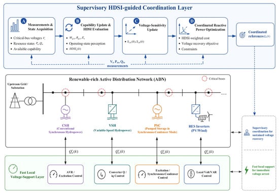
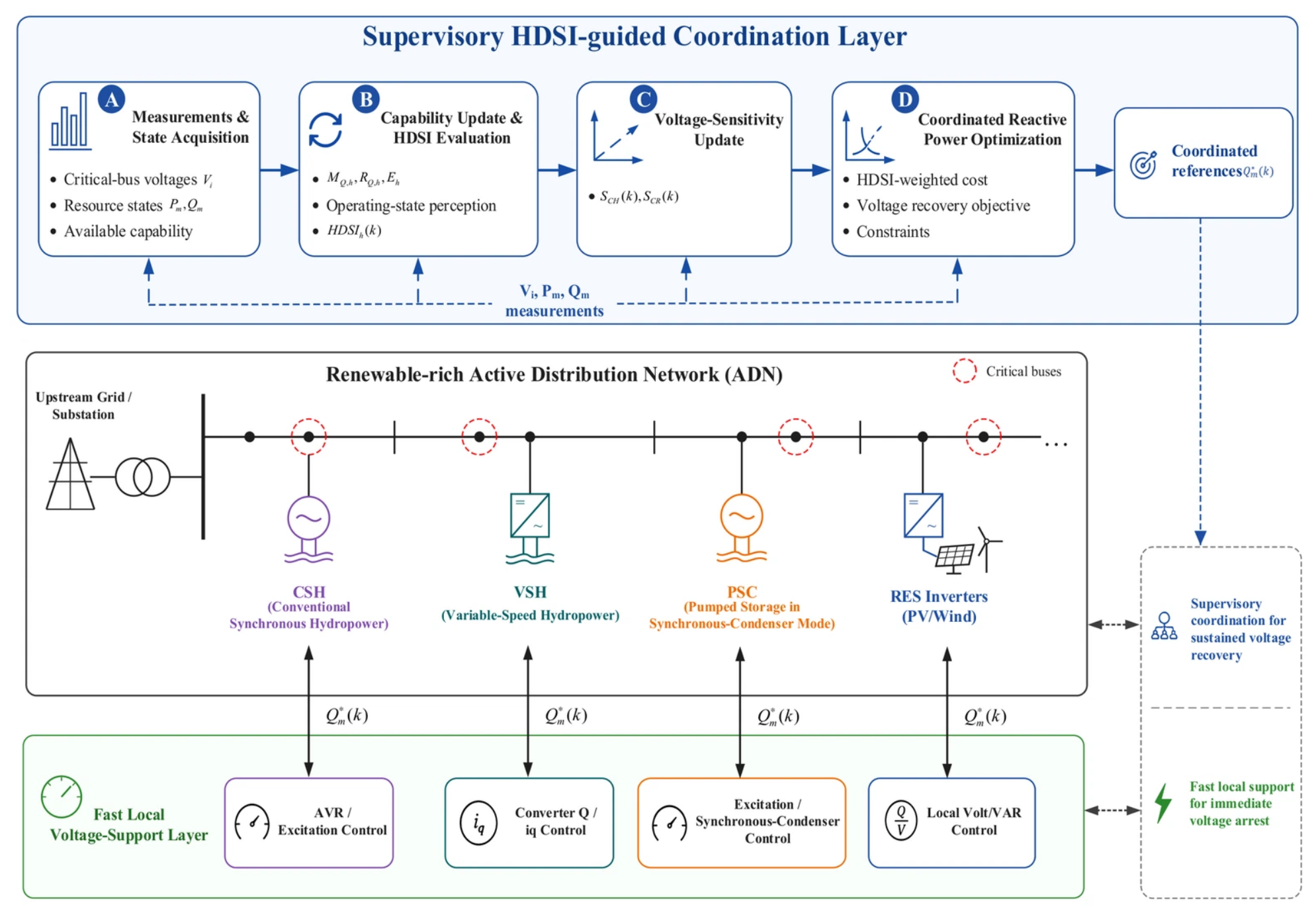
Therefore, the initial voltage response should not rely entirely on centralized coordination [22,23,24]. A fast local support–supervisory coordination architecture is adopted, as illustrated in Figure 4.

Figure 4. HDSI-guided hierarchical coordinated voltage-control architecture.

The fast local support layer acts directly through device-level controllers. For CSH and PSC units, the excitation system rapidly adjusts excitation and reactive power according to the terminal voltage deviation. For VSH units and renewable inverters, converter-based reactive power or q-axis current control provides rapid dynamic support. Because this layer does not depend on supervisory communication, it provides the first response for arresting further voltage deterioration. The supervisory coordination layer operates with a control interval T_s. The coordination center acquires critical bus voltages, the current P/Q operating states of hydropower and renewable resources, and the available resource capability. The HDSI_h(k) of each hydropower resource is then updated using the method developed in Section 3. Based on these quantities, the supervisory optimizer calculates additional reactive power adjustments for the available resources.

Let the set of all controllable reactive power resources be Ω_U = Ω_H ∪ Ω_R, where Ω_H and Ω_R denote the hydropower-resource set and renewable-inverter set, respectively. For resource m ∈ Ω_U, the coordinated reactive power target at supervisory interval k is

$$Q_m^{*}(k)=Q_m(k)+\Delta Q_m^{\mathit{sup}}(k).$$

(29)

Here, Q_m(k)denotes the measured reactive power output, which already includes the fast local support, and $\Delta Q_m^{\mathit{sup}}(k)$ is the additional supervisory adjustment. Importantly, $Q_m^{*}(k)$ represents a commanded reference rather than the reactive power instantaneously delivered to the network. In the implemented controller-level simulation, this reference is coordinated with the fast local voltage support request, and the actual reactive power output evolves according to the device-specific first-order dynamics, ramp-rate limits, and capability saturation. The device states are updated at a 1 ms simulation step, while the supervisory references are updated every 50 ms. Therefore, the optimized increment is applied as a device reference and is not directly imposed as the actual reactive power injection at the next supervisory instant.

4.2. HDSI-Guided Coordinated Reactive Power Optimization

The principal task of supervisory coordination is to allocate incremental reactive power among available resources according to the current voltage condition while respecting their dynamic capability constraints. To ensure that the HDSI directly influences the control decision, it is embedded in the hydropower regulation cost rather than being used merely as a pre-dispatch ranking criterion.

At supervisory interval k, let the incremental reactive power vectors of hydropower resources and renewable inverters be denoted by ΔQ_H(k) and ΔQ_R(k), respectively. Based on the voltage–reactive power sensitivity relationship established in Section 2.1, a quasi-static voltage estimate associated with the supervisory reactive power increments is obtained as

$${\widehat{V}}_C(k+1)=V_C(k)+S_{\mathit{CH}}(k)\Delta Q_H(k)+S_{\mathit{CR}}(k)\Delta Q_R(k),$$

(30)

where V_C(k) is the current critical bus voltage vector, while S_CH and S_CR denote the hydropower-to-critical bus and renewable-to-critical bus submatrices extracted from S_VQ, respectively.

Equation (30) is a quasi-static voltage-sensitivity approximation used for computationally efficient supervisory coordination. It evaluates the voltage effect of the commanded reactive power increments without explicitly incorporating their finite delivery rates; therefore, the estimated voltage change may differ from the actual change within one 50 ms interval. For example, the first-order CSH model with a 0.200 s time constant delivers approximately 22% of a reference step within 50 ms before ramp limitations are considered. In the closed-loop simulation, this response lag is explicitly represented by the discretized device dynamics rather than being eliminated by the ramp constraint in Equation (34). The resulting prediction mismatch is quantitatively assessed in Section 5.3.

To give a hydropower resource with a high HDSI a greater tendency to participate in the coordinated response, its HDSI-dependent regulation-cost coefficient is defined as

c_h(k) = ε_c + 1 − HDSI_h(k),  h ∈ Ω_H,

(31)

where ε_c > 0 is a small positive constant. Because the revised normalization guarantees 0 ≤ HDSI_h(k) ≤ 1 throughout the feasible operating envelope, the HDSI-dependent regulation-cost coefficient satisfies ε_c ≤ c_h(k) ≤ 1 + ε_c,  ε_c > 0. Therefore, the regulation-cost coefficient remains strictly positive for all feasible reactive power operating points, including those involving reactive power absorption. A resource with a higher HDSI receives a lower but strictly positive regulation penalty, which preserves the intended continuous resource-allocation mechanism.

Accordingly, HDSI_h(k) ↑   ⇒ c_h(k)↓. Hence, a resource with a larger dynamic support value incurs a lower marginal regulation penalty and is naturally assigned a larger share of the coordinated reactive power when beneficial. Unlike hard priority-based dispatch, this formulation preserves continuous optimization and allows multiple resources to participate simultaneously according to their capabilities and electrical locations.

Considering critical bus voltage recovery, hydropower support value, renewable-inverter utilization, and control smoothness, the supervisory objective is formulated as

$$\begin{array}{l}{\min }_{\Delta Q_H,\Delta Q_R,{\xi }^{+},{\xi }^{-}}J(k)={\lambda }_V{‖W_V\left[{\widehat{V}}_C(k+1)-V_C^{\mathit{ref}}\right]‖}_2^2+{\lambda }_H{\displaystyle \sum _{h\in {\mathrm{\Omega }}_H}{c}_h}(k){\left[\Delta Q_h(k)\right]}^2\\ +{\lambda }_R{‖W_R\Delta Q_R(k)‖}_2^2+{\lambda }_{\Delta }{‖\Delta Q(k)-\Delta Q(k-1)‖}_2^2+{\lambda }_{\xi }\left({‖{\xi }^{+}‖}_2^2+{‖{\xi }^{-}‖}_2^2\right)\\ \Delta Q={\left[\Delta Q_H^T,\Delta Q_R^T\right]}^T\end{array}.$$

(32)

The first term minimizes the critical bus voltage deviation, with W_V representing the critical bus weighting matrix. The second term is the HDSI-weighted hydropower regulation cost and constitutes the principal coupling between capability assessment and coordinated control. The third term limits excessive reactive power utilization of the renewable inverters, where W_R may reflect their remaining capability or regulation cost. The fourth term suppresses abrupt variations in consecutive coordination commands, while the last term penalizes voltage-constraint relaxation. The coefficients λ_V, λ_H, λ_R, λ_Δ, and λ_ξ are nonnegative weighting factors.

During or immediately after a severe fault, some critical bus voltages may temporarily lie outside the normal operating range. Directly imposing hard voltage limits could therefore make the coordination problem infeasible. Nonnegative slack variables ξ⁺ and ξ⁻ are introduced:

$$V_C^{\mathit{min}}-{\xi }^{-}\le {\widehat{V}}_C(k+1)\le V_C^{\mathit{max}}+{\xi }^{+},\hspace{1em}{\xi }^{+},{\xi }^{-}\ge \mathbf{0}.$$

(33)

A sufficiently large λ_ξ ensures that the slack variables are activated only when the normal voltage limits cannot be satisfied. This preserves feasibility under severe disturbances without weakening the voltage-security requirement during normal operation.

For hydropower resource h, the supervisory reactive power increment is jointly constrained by its current reactive capability and response rate. Define

$$\begin{array}{l}\Delta Q_h^{\mathit{min}}(k)=\max \left[Q_h^{\mathit{min}}(k)-Q_h(k),-R_{Q,h}^{\mathit{max}}{T}_s\right]\\ \Delta Q_h^{\mathit{max}}(k)=\min \left[Q_h^{\mathit{max}}(k)-Q_h(k),R_{Q,h}^{\mathit{max}}{T}_s\right]\\ \Delta Q_h^{\mathit{min}}(k)\le \Delta Q_h(k)\le \Delta Q_h^{\mathit{max}.}(k),\hspace{1em}h\in {\mathrm{\Omega }}_H\end{array}.$$

(34)

For CSH and PSC units, $Q_h^{\mathit{min}}/Q_h^{\mathit{max}}$ are determined by excitation and machine capability limits. For VSH units, the dynamic reactive power boundary additionally depends on the current active power operating point and converter-current limit. Equation (34) limits the admissible supervisory reactive power increments but does not eliminate the finite response lag of the devices. In the actual closed-loop simulations, the commanded references are tracked through the first-order device dynamics with explicit ramp-rate and reactive power saturation limits. Therefore, the supervisory voltage estimate should be interpreted as an approximate coordination signal rather than a strict guarantee of next-step voltage-limit satisfaction.

For renewable inverter r, its active power output is treated as known over one supervisory interval. The available reactive power limit is

$$\begin{array}{l}{Q}_r^{\mathit{lim}}(k)=\sqrt{S_r^2-P_r^2(k)}\\ -Q_r^{\mathit{lim}}(k)-Q_r(k)\le \Delta Q_r(k)\le Q_r^{\mathit{lim}.}(k)-Q_r(k),\hspace{1em}r\in {\mathrm{\Omega }}_R\end{array}.$$

(35)

Equation (35) represents the nominal apparent power capability of renewable inverters under prescribed active power operation. It effectively adopts an active power-priority allocation, with reactive power constrained by the remaining nominal capacity. However, the present controller-level model does not explicitly incorporate PCC-voltage-dependent current saturation, fault-period reactive-current priority, or active power curtailment. Therefore, Equation (35) should not be interpreted as a guarantee of instantaneous converter-current feasibility during deep voltage sags. The supervisory optimizer allocates reactive power within the adopted nominal capability boundaries according to the HDSI values, network sensitivities, and available resources.

Equations (30)–(35) therefore constitute the proposed HDSI-guided incremental reactive power coordination model. Importantly, the HDSI does not prescribe the reactive power output of an individual resource. Instead, it modifies the marginal regulation cost through (31) and (32).

5. Case Studies

5.1. Test System and Simulation Setup

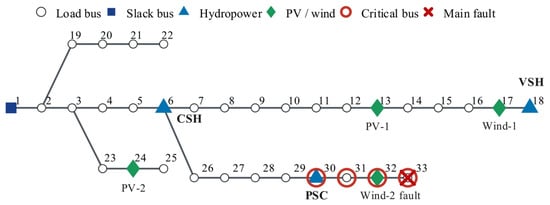
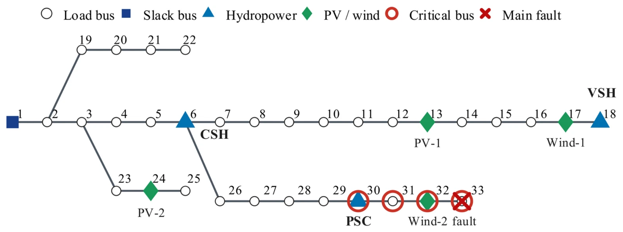
To evaluate the proposed operating-state-aware HDSI and hierarchical coordinated voltage-control strategy, a modified IEEE 33-bus active distribution network is implemented in MATLAB 2024b. As shown in Figure 5, the base voltage and base power are 12.66 kV and 10 MVA, respectively, with a nominal load of 3.715 MW/2.300 Mvar. The CSH, VSH, and PSC units are connected to buses 6, 18, and 30, while PV-1, PV-2, Wind-1, and Wind-2 are connected to buses 13, 24, 17, and 32, respectively. The critical bus set is Ω_C = {30,31,32,33}.

Figure 5. Configuration of the modified IEEE 33-bus active distribution network used for case studies.

The renewable penetration level in the main case is 40%, with active power allocation shares of 0.24/0.26/0.22/0.28. The main system and controller parameters are summarized in Table 2. Figure 5 also identifies the heterogeneous hydropower resources, renewable units, critical buses, and main-fault location.

Table 2. Main parameters of the test system and coordinated controllers.

Parameter	Symbol	Value	Unit
Base voltage/power	Vbase/Sbase	12.66/10	kV/MVA
Nominal active/reactive load	PL/QL	3.715/2.300	MW/Mvar
Hydropower buses (CSH/VSH/PSC)	ΩH	6/18/30	–
RES buses (PV-1/PV-2/Wind-1/Wind-2)	ΩR	13/24/17/32	–
Critical bus set	ΩC	({30,31,32,33})	–
Hydropower rated apparent powers	SH	1.50/1.20/1.50	MVA
Initial hydropower active powers (main case)	PH,0	0.975/0.360/0	MW
Hydropower reactive power limits (main case)	[QH,min,QH,max]	[−0.55, 0.80]/[−0.60, 1.145]/[−1.00, 1.20]	Mvar
Hydropower time constants	τH	0.200/0.025/0.100	s
Local gains/ramp limits	KH/rH	0.34/0.25; 0.55/2.50; 0.42/0.45	–/p.u./s
Main-case RES penetration	ηRES	40	%
RES power factor/time constant	pfRES/τRES	0.86/0.020	–/s
Main fault	nf,tf/tc,Zf	33, 0.50/0.60, (0.050 + j0.050)	–/s/p.u.
Simulation step/horizon	Δt/Tsim	0.001/3.0	s
Supervisory control period	Tsup	0.050	s
HDSI parameters	DV,sat/κ	0.10/10	p.u./–
QP weighting factors	λV/λH/λRES/λΔ	1400/200/80/1.8	–

Note: The VSH reactive power upper limit depends on its active power operating point and is recalculated for each scenario. The values reported here correspond to the representative main-fault scenario.

The rated apparent powers of the CSH, VSH, and PSC units are 1.50, 1.20, and 1.50 MVA, respectively. In the representative main-fault scenario, their active power outputs are 0.975, 0.360, and 0 MW, respectively. For the VSH unit, the reduced active power loading increases its nominal reactive power capability to $\sqrt{{1.20}^2-{0.360}^2}=1.145$ Mvar, compared with 0.960 Mvar at the default 0.720 MW operating point. The VSH capability limit is recalculated according to the active power operating point of each scenario. The reactive power time constants of the three hydropower resources are set to 0.200, 0.025, and 0.100 s, respectively. Both local reactive power regulation and supervisory coordination are constrained by the scenario-specific capability limits, which are also enforced during the device-level dynamic updates.

The main disturbance is a three-phase symmetrical fault at bus 33, initiated at t_f = 0.50 s and cleared at t_c = 0.60 s, with Z_f = 0.050 + j0.050 p.u. The simulation horizon is 3.0 s with a fixed integration step of 0.001 s. Fast local controllers are updated at each simulation step, whereas HDSI evaluation and supervisory coordination are executed every T_sup = 0.050 s, thereby establishing a clear two-timescale control structure. The reference and recovery-threshold voltages are 1.00 and 0.95 p.u., respectively. Voltage recovery is declared only when all critical bus voltages remain above 0.95 p.u. for at least 0.10 s. The HDSI severity saturation and membership-smoothing parameters are set to D_V,sat = 0.10 and κ = 10, respectively. The principal QP weighting factors are 1400/200/80/1.8.

A total of 120 calibration scenarios and 60 independent validation scenarios are generated using separate random seeds of 2026 and 12,026, respectively. The calibration ranges include renewable penetration of 20–70%, load scaling of 0.8–1.2, fault durations of 30–100 ms, and VSH active power loading of 30–90%. Fault locations are uniformly selected from buses 12, 18, 22, 25, 29, and 33. The fault impedance is z(0.75 + j0.25), where z is uniformly sampled from 0.05 to 0.15 p.u. Hydropower reactive capability, response time, and ramp-limit multipliers are sampled from 0.65–1.00, 0.25–4.00 (log-uniform), and 0.35–2.00, respectively.

The normalization reference bounds for M_Q, R_Q, and E are [0,1], [0,1], and [0,0.45], respectively. The ADSC target bounds for mild regulation, voltage arrest, and voltage recovery are [0,0.719741], [0,0.210259], and [0,0.286917], respectively. These state-specific ADSC normalization bounds are determined exclusively from the 120 calibration scenarios and subsequently applied unchanged to the 60 independent validation scenarios, thereby preventing information leakage between calibration and validation.

The fitted weight vectors, ordered as (M_Q,R_Q,E), are ω^M = (0.225872,0.133519,0.640609), ω^A = (0.393841,0.199277,0.406882), and ω^R = (0.245105,0.154731,0.600164). The fixed-weight comparator C2 uses their arithmetic mean, ω^F = (0.288273,0.162509,0.549218), without online state-dependent updating.

5.2. HDSI Assessment and Validation

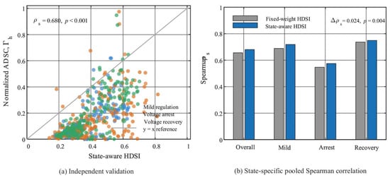
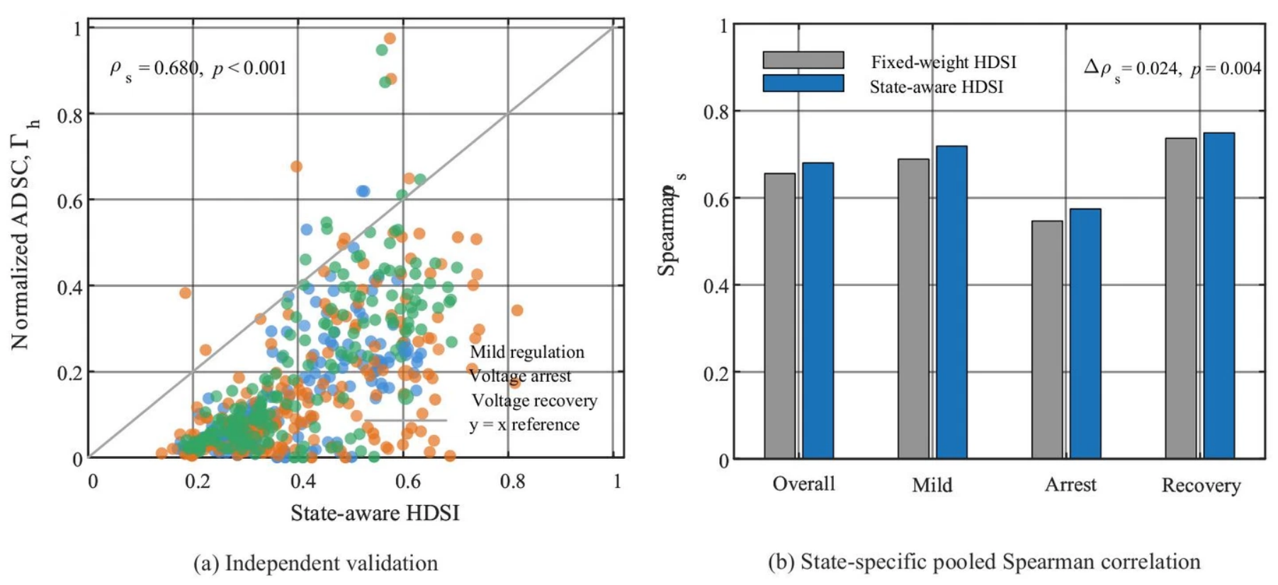
To evaluate whether the proposed HDSI accurately represents the actual dynamic support value of heterogeneous hydropower resources, 60 validation scenarios that are completely independent of the 120 calibration scenarios are first considered. Figure 6 shows the relationship between the state-aware HDSI and the normalized actual dynamic support contribution (ADSC). The validation samples cover the mild-regulation, voltage-arrest, and voltage recovery states. Across the 540 pooled resource–scenario–state samples, the proposed state-aware HDSI achieves a Spearman correlation of ${\rho }_s^{\mathit{pool}}=0.680$ with normalized ADSC (p < 0.001), which indicates a positive overall monotonic association. This pooled correlation evaluates the representation of the relative support value across different operating conditions and should not be interpreted as a direct measure of resource-ordering accuracy within an individual scenario. The y = x line in Figure 6a is included only as a visual reference, as HDSI is intended for relative resource-value assessment rather than direct numerical regression of ADSC.

Figure 6. Validation of the proposed HDSI against actual dynamic support contribution.

Table 3 further compares the capacity-only index, spatial-sensitivity index, fixed-weight HDSI, and proposed state-aware HDSI. The capacity-only metric yields a Spearman coefficient of only 0.348. Although spatial sensitivity achieves relatively high Top-1 identification accuracy, its overall rank correlation remains limited to 0.399. These results indicate that both capacity and electrical location provide useful information but are insufficient individually to characterize dynamic support value. As summarized in Table 3, the proposed state-aware HDSI increases the pooled Spearman correlation from 0.655 to 0.680 compared with the fixed-weight HDSI. The improvement of 0.0244 is supported by a scenario-clustered paired bootstrap analysis (95% CI: [0.0103, 0.0384]; (p = 0.004)). However, this improvement concerns pooled resource-value association rather than within-scenario resource ordering. When Spearman correlations are calculated separately for each of the 180 scenario–state groups and then averaged, the fixed-weight and proposed methods yield 0.778 and 0.772, respectively. Both methods achieve the same Top-1 accuracy of 81.1%, while the fixed-weight method exhibits slightly higher ranking consistency (86.7% versus 85.9%) and lower mean rank error (0.267 versus 0.281). Therefore, the proposed method does not establish superior within-scenario ordering accuracy. Its demonstrated advantage lies in a stronger pooled monotonic association between HDSI and ADSC across operating conditions while maintaining broadly comparable within-scenario ranking performance.

Table 3. Independent validation of alternative indices and the proposed state-aware HDSI.

Index	Spearman ρs	Top-1 Accuracy	Ranking Consistency	Mean Rank Error
Capacity only	0.348	62.8%	68.3%	0.604
Spatial sensitivity only	0.399	85.0%	69.3%	0.583
Fixed-weight HDSI	0.655	81.1%	86.7%	0.267
Proposed state-aware HDSI	0.680	81.1%	85.9%	0.281

The proposed method does not dominate every discrete ranking metric. Spatial sensitivity achieves the highest Top-1 accuracy, while the fixed-weight HDSI yields slightly better ranking consistency and mean rank error. The principal advantage of the proposed HDSI is therefore its improved global monotonic representation of relative resource value across changing operating states while maintaining comparable discrete ranking performance. This property is consistent with its subsequent use as a continuous weighting signal in the coordinated optimization rather than merely as a selector of the single highest-ranked resource.

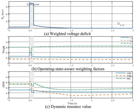
Figure 7 illustrates the online evolution of the HDSI during the main disturbance. Following fault inception, the weighted voltage deficit D_V increases sharply and subsequently decays after fault clearance. Meanwhile, the relative importance of the three support dimensions changes continuously. During severe voltage deterioration, reactive power availability and response capability become more important, while the relative weight of spatial effectiveness is temporarily reduced. The weighting factors are redistributed again during the subsequent voltage recovery process.

Figure 7. Dynamic evolution of operating-state-aware weights and HDSI following the main disturbance.

These changes are further reflected in the HDSI trajectories of the CSH, VSH, and PSC resources. Their dynamic support values evolve differently during fault arrest and recovery, which confirms that the HDSI is not a fixed resource-type score but rather a state-dependent quantity jointly determined by the resource operating condition and the evolving system requirement.

5.3. Comparative Performance of Coordinated Voltage Control

Four control strategies are compared to evaluate the closed-loop benefit of incorporating the HDSI into supervisory coordination: C0 uses only local device-level control; C1 employs a uniform-cost QP; C2 incorporates a fixed-weight HDSI; and C3 represents the proposed state-aware HDSI-guided hierarchical control. C1–C3 use identical network models, dynamic capability constraints, and voltage-control objectives, with the resource-value weighting mechanism being the principal difference.

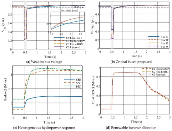
Figure 8a shows the voltage response of the weakest critical bus, bus 33. The fault-period voltage minima are nearly identical for all four strategies, with V_min,fault equal to 0.2305, 0.2306, 0.2306, and 0.2306 p.u. for C0–C3, respectively. This indicates that the instantaneous voltage nadir is primarily determined by the fault severity and fast local response rather than by the 50 ms supervisory layer. The differences emerge mainly during post-fault voltage recovery.

Figure 8. Dynamic voltage response and reactive power allocation under different control strategies.

The recovery time decreases from 0.344 s under C0 to 0.187, 0.173, and 0.172 s under C1, C2, and C3, respectively. The proposed strategy therefore reduces the recovery time by 50.0% relative to local control and by approximately 8.0% relative to the uniform-cost QP. Meanwhile, J_V decreases from 0.06841 p.u.·s under C0 to 0.06552 p.u.·s under C3. Figure 8b further confirms that all critical buses recover above the specified 0.95 p.u. threshold under the proposed method.

Under the representative main fault, C2 and C3 exhibit very similar voltage trajectories. The corresponding closed-loop voltage-control performance and resource-utilization metrics for all four control strategies are summarized in Table 4. As reported in Table 4, compared with C2, C3 reduces the total incremental reactive power effort from 0.8145 to 0.8129 p.u.·s and decreases hydropower saturation exposure from 2.219 to 1.933 unit·s, corresponding to a 12.9% reduction. This result demonstrates improved resource utilization under the representative disturbance, while its consistency across different operating conditions is further examined through the paired robustness analysis in Section 5.5.

Hydropower saturation exposure is defined as the time integral, from fault initiation to the end of the simulation, of the number of hydropower resources whose reactive power outputs reach at least 99% of their scenario-specific upper reactive power limits. Figure 8c shows the differentiated reactive power responses of the CSH, VSH, and PSC resources. The peak VSH reactive power output under C3 is 1.142 Mvar, remaining below the scenario-specific upper limit of 1.145 Mvar. Figure 8d further indicates similar aggregate renewable-inverter support among the three coordinated strategies.

The corresponding RES reactive power utilizations are 0.674, 0.680, and 0.682 for C1–C3, respectively, which indicates that the lower hydropower saturation achieved by C3 results from a modest redistribution of reactive support rather than a uniform reduction in resource utilization.

Table 4. Closed-loop voltage-control performance and resource utilization under the main fault.

Method	Vmin,fault (p.u.)	Trec(s)	JV (p.u.·s)	Total ▲ Q Effort (p.u.·s)	Hydro Saturation (Unit·s)	RES Q Utilization	Mean tQP (ms)	Convergence
C0 Local only	0.2305	0.344	0.06841	0.5223	0.000	0.723	—	100.0%
C1 Uniform-cost QP	0.2306	0.187	0.06572	0.8156	2.121	0.674	1.905	100.0%
C2 Fixed HDSI	0.2306	0.173	0.06553	0.8145	2.219	0.680	0.734	100.0%
C3 Proposed state-aware HDSI	0.2306	0.172	0.06552	0.8129	1.933	0.682	0.756	100.0%

Table 4. Closed-loop voltage-control performance and resource utilization under the main fault.

Method	Vmin,fault (p.u.)	Trec(s)	JV (p.u.·s)	Total ▲ Q Effort (p.u.·s)	Hydro Saturation (Unit·s)	RES Q Utilization	Mean tQP (ms)	Convergence
C0 Local only	0.2305	0.344	0.06841	0.5223	0.000	0.723	—	100.0%
C1 Uniform-cost QP	0.2306	0.187	0.06572	0.8156	2.121	0.674	1.905	100.0%
C2 Fixed HDSI	0.2306	0.173	0.06553	0.8145	2.219	0.680	0.734	100.0%
C3 Proposed state-aware HDSI	0.2306	0.172	0.06552	0.8129	1.933	0.682	0.756	100.0%

The influence of the quasi-static supervisory predictor was further examined using the recorded closed-loop trajectories. For the main disturbance, retrospective one-step voltage prediction over 48 post-fault supervisory intervals yielded a mean absolute error of 0.00124 p.u. and a maximum error of 0.00272 p.u. across the four critical buses. The actual post-fault voltage-limit violation rate was 6.98% over the 0.6–3.0 s observation period, with all violations confined to the initial recovery interval ending at 0.771 s. No further voltage violations were observed after 0.8 s. These results indicate that the simplified supervisory approximation can support effective closed-loop voltage recovery when combined with explicit device-level dynamics and fast local control. Nevertheless, the predictor does not provide a strict one-step voltage-feasibility guarantee, particularly during rapid disturbances or under binding device constraints.

All coordinated strategies achieve 100% optimization convergence. The mean QP solution time of C3 is 0.756 ms, substantially below the 50 ms supervisory interval. The main-fault results therefore demonstrate that the proposed strategy preserves effective post-fault voltage recovery while reducing excessive hydropower saturation, without introducing a significant computational burden.

5.4. Ablation and Parameter Sensitivity Analysis

To examine the necessity of the three HDSI dimensions, the dynamic reactive power margin M_Q, response capability R_Q, and spatial effectiveness E are individually removed. For each ablated model, the remaining weighting factors are recalibrated using the same calibration dataset and constraints as the complete HDSI to ensure a fair comparison.

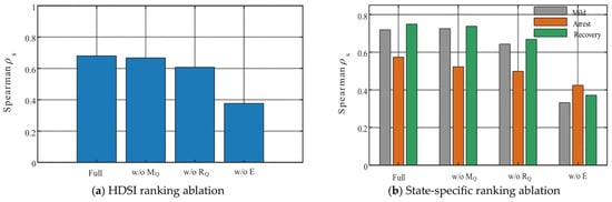
As shown in Figure 9a and Table 5, the complete HDSI achieves a Spearman coefficient of 0.680. Removing M_Q decreases the coefficient to 0.667, corresponding to a 1.9% reduction. Removing R_Q reduces it to 0.607, whereas removing E produces the most pronounced degradation to 0.376, corresponding to a 44.7% decrease. All three dimensions therefore contribute to resource-value assessment, with spatial electrical effectiveness being particularly important in the radial ADN considered in this study.

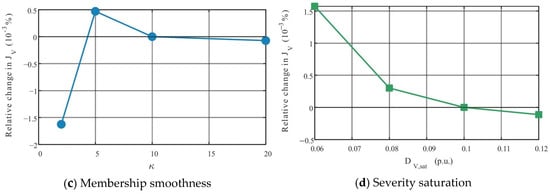
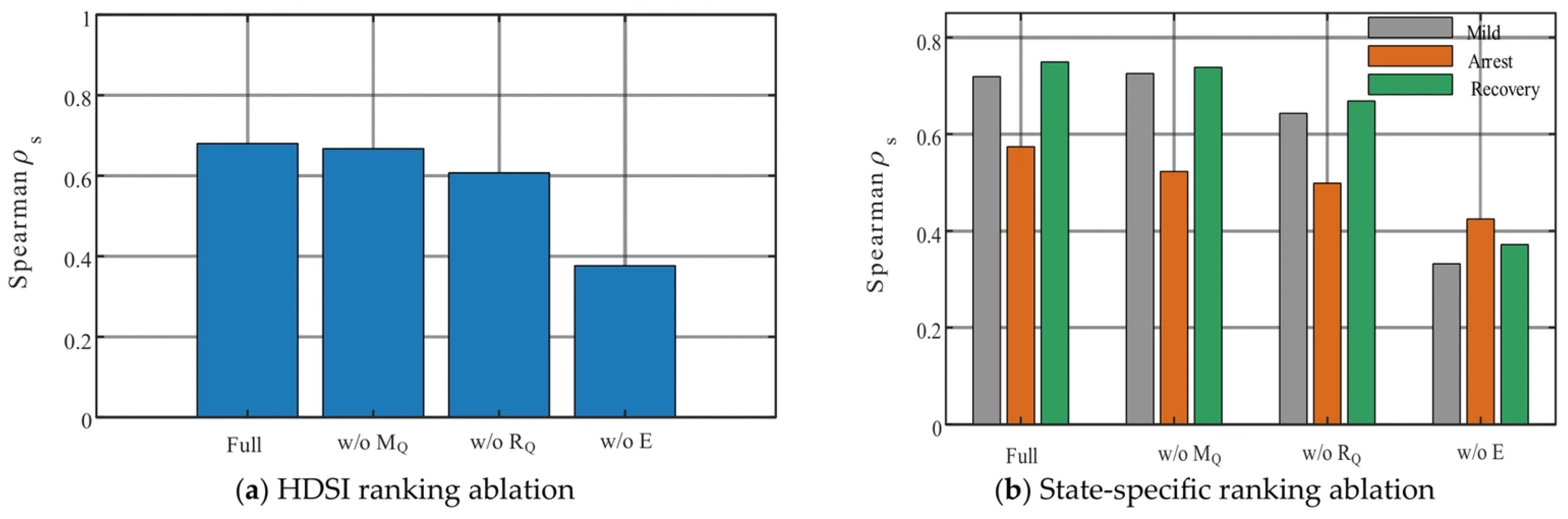
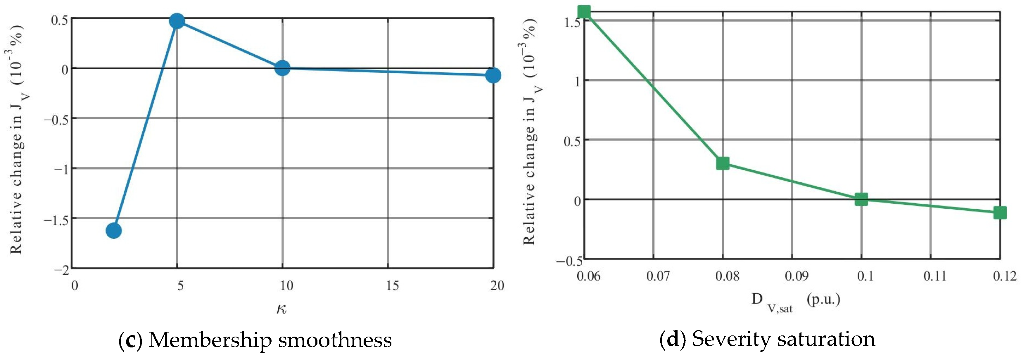
Figure 9. Ablation and parameter-sensitivity analysis of the proposed HDSI.

Table 5. Ablation results of the HDSI dimensions.

Variant	Spearman ρs	Decrease in ρs	Mean JV (p.u.·s)	Std. JV (p.u.·s)	Median Trec(s)
Full HDSI	0.680	0.0%	0.02699	0.02314	0.258
w/o MQ	0.667	1.9%	0.02701	0.02315	0.258
w/o RQ	0.607	10.7%	0.02699	0.02313	0.258
w/o E	0.376	44.7%	0.02689	0.02313	0.247

The state-specific results in Figure 9b further show that the influence of each dimension varies across the mild-regulation, voltage-arrest, and voltage recovery states. Removing response capability noticeably degrades ranking performance during disturbance-related states, whereas removing spatial effectiveness causes substantial degradation across all three states.

The closed-loop J_V and T_rec values in Table 5 remain relatively close among the different ablation variants, and some simplified variants even produce marginally lower values for an individual voltage metric. This does not imply that the removed dimension is unnecessary. All variants retain the same voltage regulation and reactive capability constraints, which allows the closed-loop optimizer to partially compensate for ranking errors. The principal purpose of the ablation analysis is therefore to evaluate the fidelity of resource-value identification rather than to require every removed dimension to cause pronounced closed-loop voltage deterioration.

Figure 9c,d further examine the membership-smoothing coefficient κ and severity saturation parameter D_V,sat. Over 2 ≤ κ ≤ 20 and 0.06 ≤ D_V,sat ≤ 0.12, the relative variation in J_V remains on the order of 10⁻³%. The proposed strategy is therefore insensitive to moderate changes in these two parameters and does not rely on fine hyperparameter tuning.

5.5. Robustness and Computational Performance

The robustness of the proposed state-aware controller (C3) is evaluated using structured disturbance scenarios, randomized cases, and communication-delay stress tests. The structured test set combines three renewable penetration levels, four fault buses, and four fault durations, which results in 48 scenarios. An additional 60 randomized operating and disturbance cases are also considered. As summarized in Table 6, the control success rate of C3 is 100% for both datasets, with network convergence rates of 100% for the structured cases and 99.78% for the randomized cases. To further assess the consistency of its benefit over fixed weighting, an additional paired comparison between C2 and C3 is conducted under the same structured and randomized scenarios.

Table 6. Robustness and online computational performance of the proposed controller.

Aggregate Robustness Results
Scenario set	N	Success rate	Mean Vmin,post (p.u.)	P95 Trec (s)	Median JV (p.u.·s)	Network convergence
Structured grid	48	100.0%	0.913	0.332	0.04239	100.00%
Random cases	60	100.0%	0.914	0.496	0.02624	99.78%
Communication delay	4	100.0%	0.911	0.270	0.07655	100.00%
Representative structured disturbance cases
RES penetration	Fault bus	Fault duration (ms)	Vmin,fault (p.u.)	Vmin,post (p.u.)	Trec (s)	JV (p.u.·s)	Converged
40%	18	80	0.8322	0.9090	0.186	0.01308	100%
40%	25	100	0.8456	0.9066	0.192	0.01415	100%
40%	30	120	0.1330	0.9174	0.154	0.09950	100%
40%	33	150	0.1110	0.9219	0.142	0.11096	100%
Online QP computation time
Median (ms)	95th percentile (ms)		Maximum (ms)		Supervisory period (ms)
0.848	1.550		12.440		50.0
Paired comparison between fixed-weight and state-aware HDSI controllers
Scenario set	Metric		Mean C2	Mean C3	Mean difference (C3 − C2)	95% CI
Structured (n = 48)	Saturation exposure (unit·s)		1.961375	1.952500	−0.008875	/
Structured (n = 48)	Recovery time (s)		0.1909167	0.1908333	−0.0000833	/
Randomized (n = 60)	Saturation exposure (unit·s)		1.315183	1.307383	−0.007800	[−0.0185167, 0.0004000]
Randomized (n = 60	Recovery time (s)		0.2026187	0.2025853	−0.0000333	[−0.0002667, 0.0002000]

For the structured dataset, the mean post-fault minimum voltage is 0.913 p.u. and the 95th-percentile recovery time is 0.332 s. The corresponding values for the random dataset are 0.914 p.u. and 0.496 s. The representative 40%-RES cases in Table 6 further show substantial variations in the fault-period voltage nadir with fault location and duration. Nevertheless, the post-fault minimum voltages remain between 0.9066 and 0.9219 p.u., with recovery times between 0.142 and 0.192 s, which indicates that the coordinated controller remains effective under spatially different disturbances.

To evaluate the consistency of state-dependent weighting, C2 and C3 are compared under the same 48 structured and 60 randomized scenarios, with identical operating conditions, disturbances, and measurement-noise realizations within each pair. The differences in hydropower saturation exposure and voltage recovery time are defined as C3 minus C2, with negative values indicating improvement. As summarized in Table 6, the mean saturation exposure decreases by 0.008875 unit·s (0.45%) in the structured scenarios and 0.007800 unit·s (0.59%) in the randomized scenarios. C3 achieves lower saturation exposure in 28 structured and 31 randomized scenarios while showing identical results in 17 and 22 scenarios, respectively. For the randomized cases, 95% confidence intervals are obtained using 20,000 paired bootstrap resamples. The confidence intervals for saturation exposure and recovery time are [−0.0185167, 0.0004000] unit·s and [−0.0002667, 0.0002000] s, respectively. Both intervals include zero, which indicates that the observed average improvements are not statistically significant. Both controllers achieve voltage recovery in all tested scenarios, with negligible differences in recovery time. Therefore, the benefit of state-dependent weighting is scenario-dependent, and the 12.9% reduction observed under the representative main fault should not be interpreted as a consistent improvement across all disturbances.

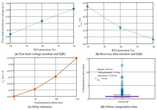
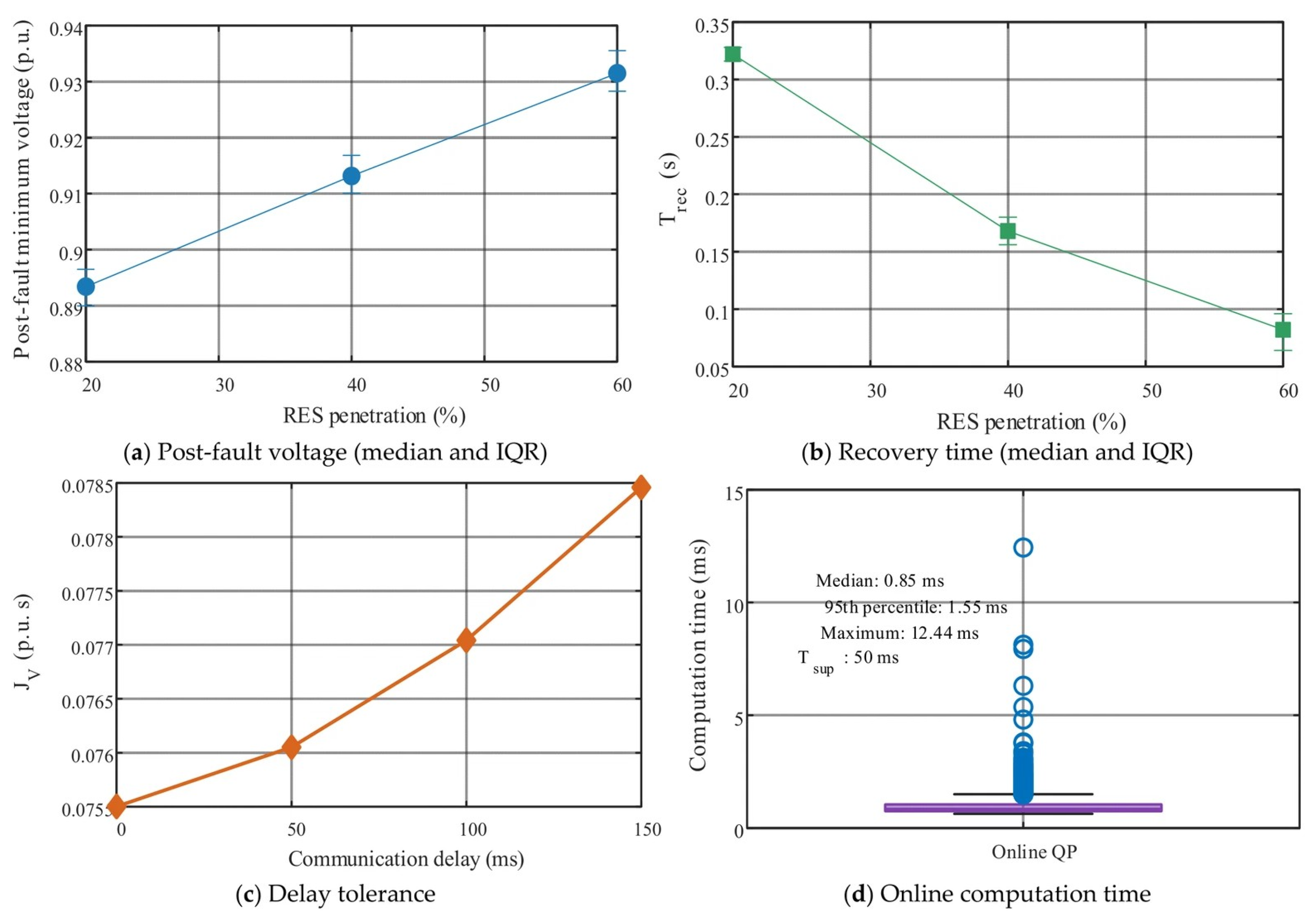
Figure 10a,b present the statistical results under different renewable penetration levels. As the renewable penetration increases from 20% to 60%, the post-fault minimum voltage increases while the recovery time decreases. This trend should be interpreted in conjunction with the inverter-sizing assumption adopted in this study: increasing renewable penetration simultaneously increases the aggregate converter-based reactive power capability. Therefore, these results do not imply that increasing renewable penetration necessarily improves voltage stability in general but rather characterize the system behavior when renewable active power penetration and available converter reactive capability increase simultaneously.

Figure 10. Robustness and online computational performance of the proposed controller.

Figure 10c evaluates the impact of communication delay. The voltage-deficit metric J_V increases monotonically as the delay is increased from 0 to 150 ms, which indicates a gradual degradation due to stale supervisory information, while all tested cases remain successfully controlled. The 100 and 150 ms cases exceed the 50 ms supervisory period and are therefore treated as stale-command stress tests rather than nominal communication conditions. The results also indicate that the fast local support layer preserves the basic voltage support function when supervisory updates are delayed.

The online computational performance is summarized in Figure 10d and Table 6. The median, 95th-percentile, and maximum QP solution times are 0.848, 1.550, and 12.440 ms, respectively, all substantially below the 50 ms supervisory interval. Even the maximum recorded solution time occupies only approximately 24.9% of one supervisory interval, providing adequate computational margin for online implementation.

Overall, the proposed controller maintains stable closed-loop performance across different renewable penetration levels, fault locations, fault durations, and communication-delay conditions. More importantly, the online computation time remains well below the supervisory update interval, which demonstrates that incorporating the state-aware HDSI does not compromise real-time feasibility.

6. Conclusions

This paper proposed an operating-state-aware hydropower dynamic support index (HDSI) and an HDSI-guided hierarchical coordinated voltage-control strategy for renewable-rich active distribution networks. By jointly considering dynamic reactive power margin, response capability, and spatial effectiveness and directly embedding the HDSI into supervisory reactive power coordination, the proposed framework couples dynamic support assessment with closed-loop voltage control. The main conclusions are as follows.

(1) The proposed HDSI effectively characterizes the operating-state-dependent dynamic support value of heterogeneous hydropower resources. Over 60 independent validation scenarios, the state-aware HDSI achieves a Spearman rank correlation of 0.680 with the actual dynamic support contribution, compared with 0.655 for the fixed-weight HDSI. The correlation improvement of 0.0244 is statistically supported by 1000 paired cluster-bootstrap resamples with p = 0.004.

(2) The HDSI-guided hierarchical controller accelerates post-fault voltage recovery while improving heterogeneous reactive resource utilization. Under the representative main fault, the recovery time is reduced from 0.344 to 0.172 s, while (J_V) decreases from 0.06841 to 0.06552 p.u.·s. Compared with the fixed-weight HDSI, the proposed method maintains a nearly identical voltage trajectory while reducing hydropower saturation exposure from 2.219 to 1.933 unit·s, corresponding to a 12.9% reduction. However, the paired robustness analysis indicates that this benefit is scenario-dependent, and no statistically significant average advantage over fixed weighting is established by the randomized tests.

(3) The proposed strategy demonstrates satisfactory robustness and real-time feasibility. A 100% control success rate is obtained for both 48 structured disturbance scenarios and 60 randomized scenarios. The median, 95th-percentile, and maximum online QP solution times are 0.848, 1.550, and 12.440 ms, respectively, all below the 50 ms supervisory interval.

Future work will extend the proposed framework to larger practical networks and electromagnetic-transient or hardware-in-the-loop platforms, with further consideration of model uncertainty, communication abnormalities, and multi-area heterogeneous resource coordination.

References

- Zhang, Z.; da Silva, F.F.; Guo, Y.; Bak, C.L.; Chen, Z. Double-layer stochastic model predictive voltage control in active distribution networks with high penetration of renewables. Appl. Energy 2021, 302, 117530. [Google Scholar] [CrossRef] [Scilit]
- Cao, D.; Zhao, J.; Hu, W.; Ding, F.; Yu, N.; Huang, Q.; Chen, Z. Model-free voltage control of active distribution system with PVs using surrogate model-based deep reinforcement learning. Appl. Energy 2022, 306, 117982. [Google Scholar] [CrossRef] [Scilit]
- Gao, Y.; Yu, N. Model-augmented safe reinforcement learning for Volt-VAR control in power distribution networks. Appl. Energy 2022, 313, 118762. [Google Scholar] [CrossRef] [Scilit]
- Pippi, K.D.; Kryonidis, G.C.; Nousdilis, A.I.; Papadopoulos, T.A. A unified control strategy for voltage regulation and congestion management in active distribution networks. Electr. Power Syst. Res. 2022, 212, 108648. [Google Scholar] [CrossRef] [Scilit]
- Zhang, W.; Sheng, W.; Liu, K.; Kang, T.; Zhan, H. Toward optimal voltage/VAR control with smart PVs in active distribution networks. Electr. Power Syst. Res. 2024, 228, 110076. [Google Scholar] [CrossRef] [Scilit]
- Meng, L.; Yang, X.; Zhu, J.; Wang, X.; Meng, X. Network partition and distributed voltage coordination control strategy of active distribution network system considering photovoltaic uncertainty. Appl. Energy 2024, 362, 122846. [Google Scholar] [CrossRef] [Scilit]
- Jiao, W.; Wu, Q.; Chen, J.; Tan, J.; Song, G.; Huang, S.; Wang, C. Analytical target cascading based real-time distributed voltage control for MV and LV active distribution networks. Int. J. Electr. Power Energy Syst. 2024, 159, 110024. [Google Scholar] [CrossRef] [Scilit]
- Zhang, Z.; Li, P.; Ji, H.; Zhao, J.; Xi, W.; Wu, J.; Wang, C. Combined central-local voltage control of inverter-based DG in active distribution networks. Appl. Energy 2024, 372, 123813. [Google Scholar] [CrossRef] [Scilit]
- Cheng, G.; Wu, X.; Yin, Z.; Zhou, J.; Qu, K. Power quality control strategy of double-layer multi-coordination for active distribution networks. Electr. Power Syst. Res. 2026, 255, 112813. [Google Scholar] [CrossRef] [Scilit]
- Xu, Z.; Deng, C.; Yang, Q. Flexibility of variable-speed pumped-storage unit during primary frequency control and corresponding assessment method. Int. J. Electr. Power Energy Syst. 2023, 145, 108691. [Google Scholar] [CrossRef] [Scilit]
- Fank, D.; Renner, H. Deployment of a full-size converter utilised hydropower plant to enhance inter-area oscillation damping. IET Gener. Transm. Distrib. 2024, 18, 1992–2005. [Google Scholar] [CrossRef] [Scilit]
- Liu, Z.; Yin, X.; Qiao, J.; Yao, W.; Yin, X.; Yang, N.; Xiao, F. Novel low voltage ride-through strategy for doubly-fed variable-speed pumped storage units using negative sequence demagnetization. Int. J. Electr. Power Energy Syst. 2026, 178, 111980. [Google Scholar] [CrossRef] [Scilit]
- Liu, X.; Xin, H.; Zheng, D.; Chen, D.; Tu, J. Transient stability of synchronous condenser co-located with renewable power plants. IEEE Trans. Power Syst. 2024, 39, 2030–2041. [Google Scholar] [CrossRef] [Scilit]
- Yuan, X.; Ma, H.; Cui, C.; Liu, M.; Gao, Z. Research on impact of synchronous condenser excitation strategy based on PIDA controller and feedforward voltage control on transient voltage of grid. Int. J. Electr. Power Energy Syst. 2024, 162, 110262. [Google Scholar] [CrossRef] [Scilit]
- Gui, Y.; Subedi, S.; Yin, Z.; Jia, W.; Wang, H. Limiter-aware adaptive excitation control for hydropower generators with legacy voltage regulation systems. Int. J. Electr. Power Energy Syst. 2026, 178, 111966. [Google Scholar] [CrossRef] [Scilit]
- Hadavi, S.; Saunderson, J.; Mehrizi-Sani, A.; Bahrani, B. A planning method for synchronous condensers in weak grids using semi-definite optimization. IEEE Trans. Power Syst. 2023, 38, 1632–1641. [Google Scholar] [CrossRef] [Scilit]
- Wu, X.; Fan, J.; Cheng, Y.; Li, W.; Tian, H.; Zhao, Z.; Hu, Z.; Li, G. Unsteady behavior of vaneless space water ring and draft-tube free surface during synchronous condenser operation of pump-turbine. J. Energy Storage 2026, 164, 122168. [Google Scholar] [CrossRef] [Scilit]
- Zhu, D.; Wang, Z.; Ma, Y.; Hu, J.; Zou, X.; Kang, Y. Hybrid LVRT control of doubly-fed variable speed pumped storage to shorten crowbar operational duration. IEEE Trans. Power Electron. 2024, 39, 14192–14203. [Google Scholar] [CrossRef] [Scilit]
- Huang, Y.; Yang, W.; Liao, Y.; Zhao, Z.; Ma, W.; Yang, J.; Yang, J. Improved transfer function method for flexible simulation of hydraulic-mechanical-electrical transient processes of hydro-power plants. Renew. Energy 2022, 196, 390–404. [Google Scholar] [CrossRef] [Scilit]
- Yang, W.; Zhao, Z.; Pérez-Díaz, J.I.; Hunt, J.D.; Vagnoni, E.; Nøland, J.K.; Quaranta, E.; Wang, R.; Li, X.; Cheng, Y. Pumped storage hydropower operation for supporting clean energy systems. Nat. Rev. Clean Technol. 2025, 1, 454–473. [Google Scholar] [CrossRef] [Scilit]
- Yan, X.; Kan, K.; Li, Y.; Li, H.; Chen, H.; Zheng, Y. Multi-scale flow and hydraulic force decomposition in a pump-turbine operating in synchronous condenser mode. Energy 2026, 360, 141821. [Google Scholar] [CrossRef] [Scilit]
- Li, Y.; Wang, Y.; Ye, H.; Xie, W.; Hua, B.; Lu, C. An integrated dynamic voltage control strategy in active distribution network based on improved model predictive control. IET Gener. Transm. Distrib. 2023, 17, 993–1006. [Google Scholar] [CrossRef] [Scilit]
- Li, Y.; Lu, C.; Tang, Y.; Fang, C.; Cui, Y. Dynamic control and time-delayed channel scheduling co-design for voltage control in active distribution networks. IEEE Trans. Smart Grid 2024, 15, 1837–1848. [Google Scholar] [CrossRef] [Scilit]
- Xu, X.; Li, Y.; Yan, Z.; Ma, H.; Shahidehpour, M. Hierarchical central-local inverter-based voltage control in distribution networks considering stochastic PV power admissible range. IEEE Trans. Smart Grid 2023, 14, 1868–1879. [Google Scholar] [CrossRef] [Scilit]
Disclaimer/Publisher’s Note: The statements, opinions and data contained in all publications are solely those of the individual author(s) and contributor(s) and not of MDPI and/or the editor(s). MDPI and/or the editor(s) disclaim responsibility for any injury to people or property resulting from any ideas, methods, instructions or products referred to in the content. |
© 2026 by the authors. Licensee MDPI, Basel, Switzerland. This article is an open access article distributed under the terms and conditions of the Creative Commons Attribution (CC BY) license.