


Abstract
Long maintenance outages require advance planning. This article presents a sequential hybrid framework for the paired phenolic joint seals of 50 generating units at the Santo Antônio Hydropower Plant, Brazil. A unit-specific long short-term memory (LSTM) model estimates the time to recorded replacement and supplies the horizon for Monte Carlo propagation using length-indexed Weibull wear models. An empirical hazard yields seal-specific outputs. Their maximum provides a signaling index based on the logical OR rule, under which either seal can trigger a signal, rather than an exact calibrated joint probability. The main historical configuration uses seven inputs, including gross head, on a 10-day grid. The corresponding archive contains 8858 forecasts across 89 of 100 selected cycles, with a pooled timing mean absolute error (MAE) of 33.58 days and disjoint network-training and validation records. Replacing arithmetic averaging with the maximum raises the mean index from 90.526% to 94.230%. A known-horizon check and a latent-wear sensitivity analysis are reported separately. A chronological calendar experiment uses fitted models held fixed during evaluation, separate development data, and a later test period containing 29 replacements. At the 90% cutoff, false-positive rates are 48.57% and 47.43% for descriptive action windows of 100 and 200 days. Precision is 8.84% and 16.89%. Higher cutoffs reduce false positives but can reduce event-warning coverage. A supervised joint-event probability extension improves Brier loss relative to a constant-risk reference while overestimating mean event risk. The results demonstrate a coupling of temporal prediction and stochastic condition projection, but do not establish an optimal cutoff, satisfactory probability calibration, or prospective operational effectiveness.
1. Introduction
Hydropower remains a major contributor to electricity supply and the operation of renewable energy systems. In 2024, it accounted for approximately 14% of global electricity generation, making it the largest individual renewable source in the generation mix reported by the International Energy Agency [1]. Maintaining this contribution requires sustained availability of generating equipment as well as adequate water resources. Within a power plant, maintenance therefore involves more than identifying a defective component: interventions must be anticipated early enough to coordinate equipment outages, spare parts, and specialized personnel. For components whose replacement requires prolonged shutdowns, the time available for this preparation is a central attribute of a useful forecast.
This operational challenge is particularly relevant in Brazil, where renewables represented 88.2% of the electricity supply in 2024, according to the Brazilian Energy Balance [2]. At the plant level, the Santo Antônio Hydropower Plant, located on the Madeira River in Porto Velho, Rondônia, comprises 50 generating units (GUs) and has an installed capacity of 3568 MW [3]. Its multi-unit configuration creates a practical need to coordinate maintenance demands across units with different condition histories. Studies of hydropower maintenance logistics have shown how crew and spare-parts configurations can be assessed through stochastic simulation [4]. Such planning benefits from component-level forecasts that indicate when an intervention may become necessary, in addition to describing equipment condition at the latest inspection.
The application considered here concerns the upper and lower phenolic joint seals associated with shaft-sealing maintenance at Santo Antônio Hydropower Plant. The available inspection records contain the residual length of each joint seal, inspection dates, and hydraulic head. In this article, wear denotes material loss, while the residual length of a seal, referred to simply as its length, denotes the measured dimension remaining after wear. The upper and lower seals are replaced together when the condition of either motivates an intervention. Consequently, the maintenance decision concerns the pair, even when the two length trajectories evolve differently. Anticipation of this shared replacement need is intended to support the preparation of long-duration outages across the generating units.
Several characteristics make this forecasting task difficult. Inspections are irregularly spaced, the observed rates of dimensional change vary across cycles, and the upper and lower seals need not exhibit the same wear behavior. Moreover, a recorded replacement is an operational event: its timing can reflect maintenance opportunities and engineering decisions as well as physical condition. A model trained on recorded replacement dates therefore estimates time to observed replacement under the historical maintenance practice.
Condition-based maintenance offers a framework for connecting inspection information to intervention planning. Hydropower reviews discuss monitoring and diagnostic methods for assessing equipment health [5,6]. For the present application, however, identifying an unfavorable current condition provides only part of the information needed by maintenance teams. They also need an estimate of the remaining planning horizon and an assessment of the plausibility of the projected condition at that horizon. This motivates a formulation that retains both a temporal prediction and an explicit representation of future dimensional wear.
Existing approaches provide complementary ways to construct such information. Mechanistic wear models relate material loss to contact mechanics, geometry, and operating conditions. For example, Xu et al. model brush-seal wear and leakage while accounting for rotor eccentricity, radial deformation, and hysteresis [7]. Their study illustrates the importance of representing seal-specific behavior, but concerns brush seals in turbomachinery rather than the phenolic joint seals studied here. Inspection-based statistical modeling offers another approach when forecasting relies on historical dimensional measurements.
Stochastic degradation models describe variability in the evolution of equipment condition and can propagate that variability into reliability or lifetime estimates. Gamma processes, for example, represent non-negative degradation increments and have been applied to hydraulic rotary-joint wear [8]. Event-based reliability formulations address a different quantity: Elusakin et al. use Weibull-distributed degradation-state transition times within a stochastic Petri-net model for offshore wind maintenance [9]. These approaches provide useful precedents for modeling uncertainty while emphasizing that a distribution of wear increments, a distribution of transition times, and a distribution of replacement times carry different interpretations.
The Weibull distribution is a widely used parametric family in reliability modeling. Since the publication that established its broad applicability [10], it has served as a reference model in reliability engineering for non-negative, right-skewed lifetime and degradation variables, because a single shape parameter spans decreasing, constant, and increasing hazard behavior and nests the exponential as a special case [11]. In maintenance applications, it describes power-transformer defect times [12], cutting-tool hazards with vibration covariates [13], degradation-state transitions in offshore wind [9], and recurrent time-to-event prediction [14]. These precedents motivate considering Weibull wear-rate models but do not establish their superiority for the present records. The choice of this family is supported by its flexibility and the descriptive fits reported from an empirical comparison with other candidate distributions, which is presented in Section 2.3.
Sequence-learning methods can extract predictive relationships from histories of condition measurements. LSTM networks provide a recurrent structure for learning temporal dependencies [15,16]. In hydropower, Wang et al. combine a comprehensive deterioration index, ensemble empirical mode decomposition (EEMD), and LSTM prediction to forecast unit degradation trends from monitoring data [17]. In machining, neural models have also been used to forecast dimensional wear and to infer remaining life from a wear-limit crossing [18,19]. Related work has examined multi-sensor and multi-model fusion for remaining-useful-life prediction of fan slewing bearings [20] and LSTM-based prediction in a dynamic multi-objective-optimization setting [21]. These studies provide examples of sequence learning and model integration across maintenance applications.
LSTM networks, Weibull distributions, Monte Carlo simulation, and empirical hazards are established methods. The principal methodological contribution of this work is their sequential integration into a replacement-forecasting architecture for paired phenolic joint seals. The LSTM does not merely accompany the stochastic model: its unit-specific time-to-replacement estimate supplies the horizon over which the Weibull-based wear trajectories are simulated. The empirical replacement hazard then converts those trajectories into seal-specific outputs at that estimated horizon, and an OR-based index represents intervention prompted by either seal. The final forecast therefore combines a temporal estimate learned from inspection histories with a stochastic assessment of seal condition at that predicted time. This coupling, and its formulation for paired seals under the plant replacement practice, distinguish the proposed methodology. No claim is made to a new LSTM cell or distribution family, or to being the first to combine neural and Weibull models.
The LSTM estimates time to recorded replacement from recent inspection sequences. Length-indexed Weibull distributions describe positive wear rates, and a truncated exponential represents small losses during intervals with zero recorded change. Censoring and mixture models support the treatment of small unresolved observations [22,23], while maximum entropy provides a rationale for choosing the exponential distribution for a specified range and mean [24,25]. Section 2.3.2 and Section 3.2 report the parameter selection and the corresponding sensitivity analysis.
The LSTM estimate sets the projection horizon, and the historical replacement hazard is applied along the simulated wear trajectories. This produces a model-derived replacement probability for each seal. Because either seal may motivate replacement of both, the maximum marginal output is the principal signaling index. The arithmetic mean remains a secondary descriptive summary of the two simulations. Identification bounds for the union event express unresolved dependence without assuming independence. Neither aggregation is presented as an exact calibrated joint probability. The aggregation comparison uses the archived historical outputs, while the latent-wear parameters are evaluated separately.
A chronological calendar experiment separates training, development, and test periods to assess false alarms, warning trade-offs, and a supervised joint-replacement probability extension. This experiment is reported separately from the historical archive and does not convert the original maximum index into an exact joint probability.
The main contributions are as follows:
- A plant-specific formulation of phenolic joint-seal replacement assessment for 50 generating units, explicitly distinguishing time to recorded replacement from time to a physical wear-limit crossing.
- An application-specific integration of unit-level LSTM time-to-replacement estimates, length-indexed Weibull wear-rate distributions, Monte Carlo simulation, and an empirical replacement hazard. The LSTM-predicted horizon controls stochastic wear propagation, linking recent condition to seal-specific model outputs and a unit-level OR index at the predicted replacement time.
- A retrospective assessment separating historical timing-error summaries, a conditional known-horizon stochastic check, and a paired comparison of seal-output aggregations. Network-training records are disjoint from validation records. A temporal-representation experiment uses an explicit chronological split. The known-horizon check is not a prospective forecast or evidence of probability calibration. A separate calendar experiment evaluates event signaling and a supervised probability extension during a later test period.
Related Work
Research on hydropower prognosis provides direct precedents for learning degradation trends, although the monitored variables and prediction targets differ from those considered here. Wang et al. construct a comprehensive deterioration index from time- and frequency-domain information and forecast it with an EEMD–LSTM model [17]. Their evaluation uses vibration data from a hydropower plant and a chronological training/test split. This supports the use of temporal models for hydropower condition assessment, but the predicted quantity is an index rather than seal length or observed replacement time. In a related energy-sector application, Le et al. investigate remaining-life prediction from vibration-derived indicators for wind turbine rotating components [26]. Such indicators are useful when direct dimensional measurements are unavailable, but their relationship to a replacement decision must be defined for each component.
Studies of physical wear make the distinction between current-state estimation and future-state forecasting particularly clear. Krupp et al. combine wear regression with autoregressive LSTM forecasting and determine remaining tool life from the predicted crossing of a wear limit [18]. Their evaluation also shows how errors in estimated current wear can propagate into future-life estimates and how changing machining conditions affect transferability. Jiang et al. use spindle power and vibration information in a wear estimator based on a residual neural network (ResNet) and an LSTM forecasting stage for subsequent drilling operations [19]. Both studies concern machining. Their relevance to phenolic seals lies in forecasting the evolution of a dimensional wear variable, rather than in a shared material, operating regime, or replacement policy.
Mechanistic and stochastic approaches offer alternative representations of the same forecasting chain. Xu et al. relate brush-seal wear and leakage to the contact configuration and demonstrate the importance of hysteresis in their experimental case [7]. Zhang et al. use a gamma degradation process with random effects to account for variation in initial condition and degradation rate when evaluating hydraulic rotary-joint reliability [8]. At the maintenance-system level, Elusakin et al. represent degradation transitions and maintenance activities through stochastic Petri nets [9].
Multi-model fusion extends this family: Liu et al. combine a nonlinear Wiener process with an Arrhenius temperature law and fuse multi-sensor temperature data through principal component analysis (PCA) into a health index for fan slewing bearings, with maximum-likelihood initialization and Bayesian online updating of the drift parameters [20]. Their formulation assumes densely sampled sensor channels, a physical law that links a measured covariate to the degradation drift, and a health index whose increments may be positive or negative. The present records consist of sparse, irregular inspections of a monotonically decreasing length, recorded in whole millimeters, with zero readings in most intervals. These conditions motivate the simpler single-family wear-rate model of Section 2.3.
These studies differ in both the physical quantity modeled and the way uncertainty enters the prediction. They therefore provide methodological comparisons rather than interchangeable models for the present seals.
Combining a recurrent network with a Weibull distribution also has precedents. Martinsson’s Weibull time-to-event recurrent neural network (WTTE-RNN) predicts Weibull time-to-event parameters from sequential covariates and accommodates censoring [14]. It differs from the present framework in the random quantity modeled: WTTE-RNN places the Weibull distribution on event time, while this study fits Weibull distributions to wear rates and uses the LSTM to supply a separate time-to-replacement estimate. Table 1 compares these formulations by their inputs, outputs, and relevance to the present application. The table provides a methodological comparison rather than a ranking of predictive accuracy across different datasets. No same-dataset benchmark against alternative forecasting architectures is reported, so the contribution lies in formulating and assessing the coupling. An accuracy advantage over existing methods has not been demonstrated.
Table 1.
Representative methodologies for degradation and replacement assessment. The other applications provide methodological analogies for phenolic joint-seal replacement.
Together, these works support the integration of sequence learning and stochastic wear modeling. The present study connects a predicted replacement horizon for paired phenolic joint seals with an explicit projection of their measured lengths. Timing error, wear-distribution fit, and replacement outputs are assessed at lead times relevant to outage planning.
The remainder of this article is organized as follows. Section 2 presents the inspection data, preprocessing, and stochastic wear and replacement-probability formulation. Section 3 is organized around the stochastic model, the LSTM predictor, and their integrated assessment. Finally, Section 4 presents the conclusions.
2. Materials and Methods
The proposed methodology combines two complementary components to assess joint-seal condition and replacement timing. A generating-unit-specific LSTM model uses recent regularized length sequences to estimate the time to replacement, in days. In parallel, a stochastic model fits Weibull distributions to observed wear rates in successive length bands, describing possible future changes in seal length.
The methodological contribution lies in the directed coupling between these components: the LSTM estimates a unit-specific horizon from the inspection sequence. That estimated horizon then determines how long each seal is propagated through its length-dependent stochastic wear model. The empirical hazard maps the simulated trajectories to seal-specific replacement outputs at the predicted horizon. The final assessment pairs the predicted time with an OR-based seal index. This is a sequential hybrid formulation, not a new recurrent cell, a new Weibull family, or an end-to-end jointly trained probabilistic model. Uncertainty in the estimated LSTM horizon is not propagated by the present conditional simulations.
The complete framework combines both components. The current inspection supplies the starting seal length, while the LSTM estimate supplies the forecast horizon. Monte Carlo realizations draw future wear from fitted Weibull distributions and project length to that horizon. A historical replacement hazard then determines absorption along each trajectory. The framework reports a time-to-replacement estimate, possible future lengths, and a model-derived probability conditional on these fitted assumptions.
2.1. Data Description and Preprocessing
The input dataset comprises inspection records for the upper and lower phenolic joint seals of the 50 generating units at the Santo Antônio Hydropower Plant. Each record includes the date of inspection, the measured residual length of each joint seal, and the corresponding gross head at the time of measurement. The data span multiple years, with irregular intervals between inspections, requiring preprocessing to ensure consistency for modeling.
Preprocessing for the reported results follows these steps:
- Filtering erroneous data: removing outliers and correcting inconsistencies in the recorded measurements.
- Cycle labeling: identifying replacements made while a seal remains in good condition, so operational decisions can be interpreted separately from wear-driven replacements.
- Causal within-cycle regularization: for the LSTM, evaluation cycles and forecast origins are identified before replay input sequences are constructed, and validation records are excluded from network training. At each forecast origin, the upper- and lower-seal histories are truncated to inspections recorded no later than that origin, and cubic-spline interpolation is then applied to the available observations to obtain the 10-day grid. Consequently, no inspection occurring after the forecast origin contributes to an interpolated LSTM input or to any feature derived from it. Interpolation is always restricted to the current wear cycle and never crosses a replacement boundary.
Before interpolation, a cycle comprising the observed inspections of the upper and lower joint seals is defined in Equation (1):
In Equation (1), denotes one wear cycle, indexes its M observed inspections, and identifies the generating unit. The cycle age is measured in days, and are the observed upper- and lower-seal lengths in millimeters, and denotes the recorded gross-head information for unit i, expressed in meters. For compactness, the notation omits the inspection index for the head information. It does not impose constant head within a cycle. The length series is regularized before model features and wear rates are computed.
Equation (2) defines the complete dataset as the union of all cycles for all generating units:
In Equation (2), is the number of retained cycles for generating unit i, is its cycle index, and is that cycle’s inspection set. The union operator ⋃ collects these sets into the complete dataset .
2.2. LSTM-Based Time-to-Replacement Modeling
2.2.1. LSTM Formulation for Time-to-Replacement Estimation
The neural component maps a sequence of joint-seal measurements to a time-to-replacement estimate in days. An LSTM network is a recurrent neural network that maintains a memory state while processing successive observations. Its gates control which information is retained, updated, and exposed to the output, allowing earlier measurements to inform the interpretation of the latest condition [15,16]. In the present application, the network combines the current length with its recent evolution: the same length can be preceded by different rates of change, even after interpolation onto a common 10-day grid.
Let q index positions within an input sequence and let denote the seven-dimensional standardized feature vector at that position, obtained from the features in Equation (4).
Equation (3) gives the conventional LSTM state update:
In Equation (3), is the logistic function for a scalar argument v, tanh is the hyperbolic tangent, and both act element-wise. ⊙ denotes element-wise multiplication. The vectors , , and are the forget, input, and output gates. is the candidate memory update, and and are the updated memory and hidden-output states. The preceding states are and . For each pathway , maps the input features, maps the preceding hidden state, and is the bias vector. With hidden width , their dimensions are , , and , respectively. All gates and states have components. These weights and biases are learned from the training sequences. The network advances through feature vectors defined on the regularized 10-day grid.
One independent network is fitted for each generating unit. Measurements from both seals enter the same network, which produces one time-to-replacement estimate for the unit rather than separate upper- and lower-seal lifetimes. The regression model supplies the replacement horizon, and the stochastic component supplies the condition-based assessment.
The following subsections describe the configuration used for the reported results: seven LSTM features including gross head and causal spline interpolation on a 10-day grid for all 50 units. The network-training and validation records are disjoint. The chronological comparison is reported separately. Section 3.4 also reports a separate archived feature-sensitivity comparison. Its results do not establish that the seven-input configuration has superior accuracy.
Figure 1 illustrates the sequence-to-one operation: each regularized feature vector updates the hidden and memory states, and the final hidden representation feeds the scalar regression layer. Figure 2 shows the gates and state variables within one recurrent step, updated by Equation (3).
Figure 1.
Unrolled LSTM sequence-to-one regression. Each regularized feature vector updates the hidden state (solid arrows) and memory state (dashed arrows). The final representation is mapped to an estimate of the time to replacement in days.
Figure 2.
Schematic LSTM cell. The gates regulate retention of previous memory, incorporation of new information, and exposure of the updated state.
2.2.2. LSTM Data Preparation, Features, and Target Construction
For each generating unit, inspection records are ordered by collection date. Records with either residual length above 18 mm are discarded. Retained negative lengths are set to zero and values between 15 and 18 mm are capped at 15 mm. Recorded replacements delimit wear cycles. Replacements made while the seals remain in good condition are identified as operational decisions and retained in the LSTM assessment, where disagreement with the wear model is informative. The last two completed cycles of each generating unit are selected for the main retrospective evaluation. The records belonging to these selected validation cycles are not used to train the LSTM networks. For a given forecast origin, the inspection history of the current cycle is first truncated to observations whose dates do not exceed that origin. Cubic-spline interpolation is subsequently performed on this truncated history to obtain the 10-day grid. The procedure is repeated independently for each forecast origin, both when constructing causal input examples and when evaluating selected historical cycles. Therefore, every regularized length and every derived LSTM feature available at a given origin depends exclusively on information that would have been available at that date. Interpolation does not cross a replacement boundary.
For grid point k in a cycle, let denote its date and and the regularized lengths.
Equation (4) defines the ordered LSTM input:
where in days, for , and . Here denotes gross head, the seventh input. Only head measurements available at the forecast origin may contribute to its construction.
The first interval and the first differences in each cycle are set to zero. Subsequent regular grid points are 10 days apart. The signed LSTM change rates differ from the non-negative material-loss rates in Equation (6). Gross head is included because the main historical timing and integrated results are reported for the seven-input configuration identified for that archive. This describes the evaluated configuration without claiming that adding head improves accuracy. A separate archived comparison of six- and seven-feature configurations is summarized in Section 3.4 and Supplementary Table S1. This separate comparison does not establish an average accuracy advantage of including gross head. The target is the number of days from the forecast origin to the recorded replacement of that cycle, rather than the time to a simulated 4 mm crossing.
2.2.3. Sequence Construction and Training per Generating Unit
A separate LSTM is used for each of the 50 generating units. In the 7-feature formulation, sequences of 4–10 regularized points are left-padded to a tensor. The architecture has one LSTM layer with 64 hidden units, dropout of 0.2, a dense layer with 16 rectified-linear units, and a scalar linear output. The documented training settings use Adam and mean squared error in standardized target space, a batch size of 16, a maximum of 300 epochs, and early stopping based on training loss with a patience of 20 epochs. Fitted networks and input/target standardizers are specific to each unit and are reused during the main replay.
The records used to train each LSTM network are disjoint from the validation records. Input and target standardizers are fitted exclusively on the corresponding training data and remain fixed during validation. The selected validation cycles do not contribute to network-weight fitting or estimation of the standardization parameters. At each forecast origin, interpolation and feature construction use only inspections available up to that date. The experiment in Section 2.2.6 likewise fits networks and scalers using preceding cycles only.
2.2.4. Inference and Validation
At each validation origin, only inspections recorded no later than that date are considered. The current-cycle history is truncated at the forecast origin and the spline is refitted using only those available observations. The resulting 10-day grid is then used to construct the most recent eligible sequence in the feature order of Equation (4), which is standardized using the corresponding unit’s archived parameters. The network output is inverse-transformed to days. On a calendar day between regular grid points, the elapsed time since the most recent grid point is subtracted from the prediction anchored at that point. This walk-forward procedure is repeated independently at every validation origin. Later inspections and the recorded replacement date do not enter interpolation, feature construction, scaling, or network inference. The replacement date is used only after prediction to compute the validation target and error.
2.2.5. LSTM Assessment and Reporting Protocol
The LSTM and integrated results in Section 3 are assessed on the two completed validation cycles of every generating unit. For each cycle, daily forecast origins run from 200 to 100 days before its recorded replacement. The main replay uses frozen networks and standardizers fitted exclusively on training records disjoint from the validation records. Although the assessment is retrospective in the sense that the replacement outcomes are already known for scoring, the information supplied to the model at each origin is strictly causal: interpolation and feature construction use only inspections available up to that date. For prediction j, define .
Equation (5) defines the pooled MAE:
Cycle-Level Error Summaries and Evaluation Criterion
For cycle c with valid origins, define and . We summarize the distribution of across evaluable cycles using its mean, median, quartiles, and interquartile range (IQR), assigning equal weight to each cycle. Separately, we report the median across cycles of their within-cycle median absolute errors. These are different summaries of prediction error. The principal criterion is days, representing approximately one month of tolerance for the mean error in the predicted replacement horizon. This descriptive evaluation criterion was not prespecified before evaluation or validated operationally by the plant. Limits of 20 and 40 days are used for descriptive sensitivity analyses and do not replace the principal criterion. A cycle without any valid forecast is non-evaluable and is never counted as meeting a criterion.
The reported percentages are calculated by dividing the number of cycles meeting the criterion either by the number of evaluable cycles or by all 100 selected cycles. Each confidence interval (CI) is estimated using 10,000 percentile-bootstrap replicates with random seed 20261014. Each replicate draws 100 whole selected cycles with replacement, preserving their origin records and multiplicities, and recomputes both percentages. In each replicate, the evaluable denominator excludes cycles without valid forecasts, while the denominator for selected cycles remains 100. The limits of the 95% interval are the 2.5th and 97.5th percentiles, using linear quantile interpolation. Daily origins are not resampled independently. As a complementary sensitivity analysis for dependence shared within a generating unit, 50 generating units are also resampled with replacement while retaining both selected cycles of each sampled unit. These intervals are conditional on the fitted networks and do not include uncertainty from retraining. Error summaries exclude non-evaluable cycles, while coverage retains all selected cycles. The pooled daily MAE weights cycles according to their numbers of valid origins. The mean cycle MAE gives equal weight to each evaluable cycle.
The number of valid origins is reported alongside the error because not every candidate day contains sufficient historical information for causal sequence construction. Daily predictions within a cycle are correlated and are therefore not treated as independent replacement events. Prospective assessment remains future work. A separate retrospective calendar evaluation of signaling and a supervised joint-event probability extension is described in Section 2.4.3.
2.2.6. Assessment of Irregular Inspection Intervals
The 10-day grid is part of the original LSTM formulation. A retrospective experiment compared this representation with an ablation using observations on their actual inspection dates and examined associations between inspection timing and prediction error. This comparison used the six length-derived and timing features in Equation (4), omitting gross head from both variants. Thus, its input tensors have six columns, while the main archived replay uses seven. In the actual-date representation (raw), is the observed interval. In the regularized representation (grid10), successive grid intervals are 10 days. Length changes are divided by the corresponding interval in each representation. The experiment evaluates temporal representation in the LSTM. It does not test sensitivity of the Weibull fits or replacement probabilities to inspection intervals.
The same measurement database and recorded replacement boundaries were used for both representations. Before sequence construction, records with either length above 18 mm were removed, retained lengths were clipped to mm, and measurements sharing a collection date were averaged in both versions. For grid10, a natural cubic spline was refitted at each origin using only the current-cycle inspections available by that date. The grid began at the first inspection and ended at the last 10-day point not later than the latest available inspection, without extrapolation. Interpolated lengths were also clipped to mm. Interpolation can update the representation of earlier lengths when another inspection becomes available, but previously issued forecasts were not recomputed using future information. Interpolated points do not constitute independent inspections.
For each unit, training was restricted to cycles completed by the beginning of its first reserved test cycle. Both test cycles were excluded from network and scaler fitting, and the fitted model was frozen for their evaluation. Eligible training origins required at least four distinct inspections and four grid points. The two representations used the same training origins and sequence widths, from four to , where the two counts refer to available actual-date and grid points. Their scalers were fitted exclusively on their respective training sequences and targets. Networks used the architecture and optimization settings of Section 2.2.3, with seed for generating unit i, matched initial weights within each pair, and no test-based hyperparameter selection. Early stopping used training loss. The resulting numbers of epochs could differ between paired models. A single seed was used per unit.
The targets for both representations referred to the same recorded replacement. Training targets were measured from the last input point of each representation. The grid anchor could precede the latest inspection by up to nine days. At inference, the horizon estimated at that anchor was bounded below by zero and the elapsed time to the daily forecast origin was subtracted. Negative remaining times after this correction were retained when scoring. Each model used its native most recent sequence of up to ten points at inference. These sequences could therefore span different physical durations or contain different numbers of points. The comparison measures the effect of these complete representations rather than isolating spline interpolation with otherwise identical input tensors.
Daily test origins again covered the 101 days from 200 to 100 days before recorded replacement. This outcome-conditioned window is retrospective. Error comparisons used only origins with valid predictions from both representations. Availability was also reported separately against all requested origins. The target construction, chronological training cutoff, date aggregation, and common training support define a distinct evaluation protocol. Its raw–grid10 contrast is directly paired, while its absolute errors do not directly reproduce those of the main LSTM evaluation in Section 3.4. Differences from the primary results cannot be attributed solely to temporal representation.
For interval analyses, the main exposure was the median or coefficient of variation (CV) of the intervals between up to the ten most recent actual inspections available at an origin. The CV is the sample standard deviation (SD) divided by the mean. Both measures were defined identically for the two representations. This describes the recent inspection cadence. The spline itself uses the full available prefix. Median intervals were grouped as , , , and >30 days. Absolute error (AE) was additionally regressed on recent-interval CV with cycle fixed effects and controls for , , and . Cycle fixed effects also absorb fixed unit differences. An analysis using one record per cycle and unit fixed effects examined cycle-wide interval statistics. These retrospective descriptors were never supplied to the networks. Sensitivity analyses excluded GU06 and GU30 and examined the paired difference in absolute error. Associations are observational and do not identify causal effects of inspection scheduling.
Confidence intervals for the paired MAE difference used 2000 bootstrap replicates resampling whole cycles. A complementary analysis resampled whole generating units with their cycles together. Uncertainty for the interval groups and regressions was likewise estimated using cluster resampling rather than independent daily observations. Groups with fewer than ten cycles or five units were flagged as having limited support, and groups with fewer than two clusters received no inferential interval. Bootstrap intervals are conditional on the fitted networks and do not quantify training-seed variability. The availability audit used collection dates, with no independent record of ingestion time or prospective forecast issuance. Perturbing inspection lengths dated after an origin did not alter its constructed inputs.
2.3. Weibull-Based Wear and Replacement-Probability Modeling
The team received joint-seal wear data covering hundreds of complete cycles, each with a known replacement date. Three observations from these cycles informed the wear-rate model:
- More than 70% of the retained 10-day grid intervals show no change in processed length. These zeros can reflect finite measurement resolution, genuinely negligible wear, and preprocessing. Their frequency is modeled separately from the distribution of positive rates.
- The initial joint-seal length is 15 mm, and replacement is preferred at 4 mm, although some seals wear below this value.
- Cycle age initially appeared to affect the wear rate, but further analysis showed that the rate depends on the length of the seal instead. Each length band therefore has its own wear-rate distribution.
The Weibull family was adopted for the nonzero wear rates based on the reliability literature, the properties of the observed rates, and an empirical comparison with competing parametric distributions. It is the established parametric model for non-negative, right-skewed reliability and degradation quantities [10,11], and the maintenance studies cited in Section 1 that use this family [9,12,13,14] adopt it for this reason. Its shape parameter represents both the concentration of very small rates and the long upper tail seen in the inspection records, the location parameter places the support at the smallest rate admitted by the fits, and the exponential is recovered as the special case . Fitting the family separately in each length band, with the zero readings described by , limits the number of parameters per band and keeps the fitted model transparent, allowing the plant team to refit it as new cycles are completed. Multi-model fusion approaches such as the nonlinear Wiener process with an Arrhenius temperature law of Liu et al. [20] were not pursued because they require densely sampled covariates, a physical degradation law, and increments that may take either sign, while the present records are sparse, integer-millimeter inspections of a monotone length with zero readings in most intervals. Furthermore, sampling wear rates directly from a nonparametric empirical distribution would remove the parametric family assumption, but it provides no probability mass beyond the largest observed rate and becomes fragile in length bands with fewer nonzero observations, motivating the retention of a three-parameter parametric family.
To empirically justify the choice of the Weibull formulation over competing parametric families, three-parameter Weibull, gamma, exponential, log-normal, and normal distributions were fitted by maximum likelihood to all pooled nonzero daily wear rates ( nonzero wear intervals out of 8962 total recorded intervals, corresponding to a zero-wear proportion of ). This pooled analysis serves as a global check across every nonzero wear rate recorded in the dataset, and the same ranking and tail behavior hold across the individual length bands defined below, which directly motivated the adoption of the Weibull distribution in this work. Table 2 summarizes the number of parameters and the maximum log-likelihood scores obtained for each distribution, and Figure 3 illustrates the corresponding probability density function (PDF) and cumulative distribution function (CDF) fits. The three-parameter Weibull distribution attained the highest log-likelihood score (), outperforming the gamma (), exponential (), log-normal (), and normal () distributions. Across the length bands, the Weibull fit closely tracks the high density of small wear rates while appropriately bounding the right tail of sparse larger increments, providing a practical and empirically supported wear model for assessment on the plant’s inspection data.
Table 2.
Empirical comparison of candidate parametric distributions fitted by maximum likelihood to the pooled nonzero daily wear rates.
Figure 3.
Comparison of fitted probability density functions (left) and cumulative distribution functions (right) for the three-parameter Weibull, gamma, exponential, log-normal, and normal distributions on the pooled nonzero daily wear rates, ranked by maximum log-likelihood. The star symbol in the legends identifies the distribution with the highest log-likelihood among the candidate models.
2.3.1. Weibull-Based Wear Modeling
The wear rate is the reduction in interpolated length between consecutive 10-day grid points divided by the elapsed time.
For cycle r and observation index i, Equation (6) defines the wear rate:
where is the interpolated length in millimeters at cycle age in days, so is expressed in millimeters per day. The stochastic-data extractor uses monotonicity correction followed by piecewise cubic Hermite interpolation (PCHIP) on a 10-day grid. These grid values provide a common time base for the recorded inspections. The final interval of each cycle is excluded from the fits.
Each wear rate is assigned to the length band that contains the length at the start of its interval.
Equation (7) defines these lower-open, upper-closed bands :
with and an open uppermost band, , although the retained lengths do not exceed 15 mm. Here, ℓ is the band index, and are the lower and upper band limits in millimeters, and M is the number of bands. Rates with are pooled across cycles. Among them, are zero, and the remaining nonzero rates form the sample . The counts and refer to usable zero and positive intervals, respectively, so their sum is the number of usable intervals in the band.
Equation (8) defines the corresponding dimensionless zero-reading probability :
A three-parameter Weibull distribution is fitted to in each band. Its parameter vector is , where is the shape, is the scale, and is the location parameter.
Equation (9) defines the probability density function (PDF):
Equation (10) defines the corresponding cumulative distribution function (CDF):
In Equations (9) and (10), x is a value at which the wear-rate distribution is evaluated in mm/day and the subscript ℓ identifies the fitted length band. The shape k is dimensionless, while the scale and location are in mm/day. The density has inverse-rate units and is zero for . The CDF is dimensionless. Admissible fitting parameters satisfy , , and , where is the smallest positive rate in the band, placing all fitted observations inside the support.
The reference for fitting is an empirical CDF built with Benard’s median-rank equation [27].
With the nonzero rates sorted as , Equation (11) assigns to the j-th ordered rate the cumulative probability
In Equation (11), j is the ordered-sample rank, is the sample size of positive rates, is the j-th ordered rate, and is its dimensionless plotting probability. These plotting positions lie strictly between zero and one, as required by the transformation used in rank regression [27,28].
Three methods provide candidate parameters in each band. The first is maximum likelihood estimation (MLE). It numerically maximizes the log-likelihood of the nonzero rates obtained from Equation (9) under the assumption of independent observations.
Equation (12) gives this log-likelihood:
In Equation (12), is the likelihood of the positive rates , with indexing those intervals. The symbol log denotes the natural logarithm. Its maximizing parameter estimate is denoted by . A hat denotes an estimated quantity.
The second, rank regression (RR) fits the Weibull CDF to the Benard positions in Weibull probability-plot coordinates, using the transformation for a cumulative probability u.
The candidate minimizes the least-squares criterion in Equation (13):
In Equation (13), is the dimensionless sum of squared discrepancies between the transformed empirical and fitted probabilities. The transformation T is defined for probabilities strictly between zero and one, and j runs over the ordered positive sample. The superscript identifies rank regression.
The third, greedy search (GS), samples admissible parameter triples within the intervals of Equation (14):
In Equation (14), the subscripts min and max denote the lower and upper search bounds for each parameter. The supplied fitting routine uses , , mm/day, , , and . Here, denotes the empirical quantile at probability p of the band’s positive rates. The scale and location bounds are therefore rate-valued. The shape bounds are dimensionless.
Each triple is scored by its Kolmogorov–Smirnov (KS) distance to the empirical step CDF [29].
Equation (15) defines that reference CDF:
In Equation (15), is the empirical step CDF of the positive rates, x is its rate threshold in mm/day, and equals one when the condition in braces holds and zero otherwise.
Considering both sides of each jump of the step CDF, the KS distance is given by Equation (16):
In Equation (16), is the largest absolute CDF discrepancy, which is dimensionless, takes the supremum over rate thresholds, and the two terms inside the maximum evaluate the right and left limits of each empirical jump.
With denoting the finite set of parameter triples evaluated in band ℓ, the search returns a best-performing evaluated triple through Equation (17):
In Equation (17), arg min denotes the set of parameter triples attaining the smallest evaluated KS discrepancy, and is a selected member of that set.
The three candidates are compared by the MAE between the fitted CDF and the Benard empirical CDF, given by Equation (18):
In Equation (18), G is the number of evaluation-grid points for the current band, indexes them, and is a rate in mm/day. The supplied routine uses a common uniformly spaced grid spanning the range from the smallest to the largest positive rate, capped at 10,000 points. The dimensionless reference is the linear interpolation of the Benard plotting probabilities. Tied rates retain their highest rank. It is distinct from the empirical step CDF used for KS scoring. The discrepancy is dimensionless.
In Equation (19), m indexes the three candidate estimators, is a method attaining the lowest CDF MAE, and is its candidate parameter vector. The selected components , , and are the fitted shape, scale, and location for band ℓ. The selection is made independently in each band, so different methods may be chosen at different lengths. The literal-zero reference is used for the descriptive wear checks, while the replacement simulation substitutes the latent branch defined below.
Equation (20) combines the zero-reading probability with the selected fit to define the reference CDF of band ℓ:
In Equation (20), is the dimensionless CDF of a draw that is zero with probability and otherwise follows the fitted Weibull distribution, with negative draws clipped at zero. is the evaluation rate in mm/day.
2.3.2. Latent Wear for Zero Readings and Replacement Hazard
Seal lengths are recorded mainly in whole millimeters. Small losses can therefore occur between identical recorded readings. The simulation represents this wear with a small positive rate when the zero-reading branch is selected. This treatment follows the use of continuous distributions for observations below a reporting limit [22,23].
Here x is a wear rate, is the exponential scale, and is the upper cutoff, all in mm/day. The CDF is zero below zero and one above the cutoff. A truncated exponential provides a simple maximum-entropy distribution for a chosen range and mean [24,25].
Equation (22) gives its mean and the sampling rule:
In Equation (22), is the mean rate in mm/day, denotes expectation, and U is a uniform random draw between zero and one.
The sensitivity study uses mm/day and mm/day. With a 10-day step, the cutoff limits loss to 0.5 mm, half the nominal recording increment, and the mean loss is 0.008 mm. The scale also controls accumulated wear during long plateaus. For the longest retained plateau, steps or 1010 days, we set a loss budget mm with target probability .
In Equation (23), denotes probability, is the rate drawn for step j, days, and and are the CDF and quantile function of a unit-scale gamma distribution with shape . Truncating the exponential draws reduces accumulated loss. Choosing mm/day gives a lower probability bound of 98.79% for staying within the plateau loss budget.
Equation (24) shows how the two wear branches contribute to the simulated mean:
Here, is the simulated rate in length band ℓ, is its zero-reading probability, and is a draw from its fitted Weibull distribution. Rates and means are in mm/day. The first term measures the wear added by the latent branch. Section 3.2 compares this setting with literal zeros, half and double the scale, alternative cutoffs, and uniform distributions. Each start-length and horizon combination uses 100,000 realizations. Historical probability summaries are presented separately in Section 3.3 and Section 3.6.
The replacement hazard is estimated from cycles ending at or below mm. Their final lengths are floored to integer levels.
For level v, counts replacements at that level, and Equation (25) counts the cycles that reached it:
Equation (26) gives the probability of replacement at a reached level:
Here, is a probability, v is the floored length in millimeters, and mm is the replacement goal. For each simulated seal, one replacement trial is drawn at its starting level and at every newly entered integer level. A successful trial terminates that trajectory.
The certain-replacement condition applies to the integer level , where L is continuous simulated residual length in millimeters. Consequently, any mm is assigned a level at or below four. This discretized hazard condition is not an exact continuous crossing of 4.000 mm. In particular, any positive loss from exactly 5 mm enters a level with certain replacement. This is the boundary effect evaluated in Section 3.2. The separate time-to-goal comparison retains its recorded-length passage convention.
2.3.3. Monte Carlo Projection of Seal Length and Replacement Probability
Monte Carlo simulation represents uncertainty in future wear by generating possible sequences of wear increments. The simulation advances in steps of days, the interval between regularized observations, so each drawn rate is held for the same span that one fitted wear rate represents. Because the wear-rate distribution depends on length, the rate for each step is drawn from the band that contains the simulated length at its start: for realization m at step d, is the simulated length and the index of its band, such that .
First, Equation (27) selects the fitted positive-rate branch or the latent branch associated with processed zero readings:
In Equation (27), N is the total number of Monte Carlo realizations, indexes them, d indexes simulation steps, and is the length-band index at the start of that realization’s step. The notation denotes a zero/one draw whose probability of one is p. Thus, equals zero with probability and one otherwise.
Second, Equation (28) draws a candidate wear rate from the band’s selected Weibull fit:
In Equation (28), is the candidate rate in mm/day before clipping. Its selected shape is dimensionless, while its scale and location have units of mm/day. Their values follow from Equation (19).
Combining both branches gives the sampled wear rate in Equation (29):
In Equation (29), is the non-negative simulated wear rate in mm/day, and is an independent latent rate in the same units drawn from Equation (21). The selector weights the clipped Weibull branch when it is one and the latent branch when it is zero. Taking the maximum with zero discards negative draws when , and draws are independent across steps and realizations.
Starting from the current length, , the simulated length is updated at each step by subtracting the wear increment, as shown in Equation (30).
In Equation (30), is the measured starting length, is the length of realization m before step d, and is its length at horizon H. All lengths are in millimeters. The horizon H is measured in whole days, is the number of simulated steps, and denotes rounding upward to an integer. Multiplying the rate by the holding time in days gives that step’s loss in millimeters. For , the step duration is , except in the last step, where holds the drawn rate for the remaining days only. When , and no wear update is performed. The update must be sequential because the band at step depends on the wear accumulated through step d.
Replacement is superimposed on the wear trajectories as an absorbing event governed by the hazard of Equation (26). Before the first step, each realization draws one Bernoulli trial with the hazard of its starting floored level, whose replacement decision may still be pending. At the end of each step, one trial is drawn for every integer level newly entered during the step, from the highest to the lowest. A success causes replacement, after which the seal stops wearing and no trials are drawn at lower levels. The indicator equals one when realization m is replaced within the horizon and zero otherwise.
The expected final length is estimated by averaging the simulated lengths, as expressed in Equation (31).
In Equation (31), N is the number of Monte Carlo realizations, indexes them, and is the arithmetic mean of their final lengths in millimeters, with replaced realizations retaining the length at which they were absorbed.
The replacement probability at the forecast horizon is the fraction of absorbed realizations, given by Equation (32).
In Equation (32), is the zero/one indicator that realization m was absorbed by horizon H, and is the dimensionless absorbed fraction, estimating the conditional replacement probability from the starting length . Evaluating the hazard along each realized trajectory, rather than on the mean length, incorporates the uncertainty in future wear. As h describes historical replacement practice, is a model-derived probability conditional on the fitted wear model and hazard.
2.4. Integration of the LSTM and Weibull Models
This subsection describes the historical integrated outputs and their reaggregation. The archived probabilities retain the configuration used in their original calculation. The latent-wear reference in Section 2.3.2 is evaluated separately and is not substituted into these archived outputs. The aggregation comparison changes only the summary across the seals. No stochastic or neural predictions are regenerated.
The two models contribute different quantities at a common forecast origin. At an eligible origin, the LSTM receives the recent sequence of regularized features and returns a time-to-replacement estimate in days, , which, rounded to whole days, defines the forecast horizon H. The current length initializes the stochastic model. The LSTM does not generate wear increments, and the Weibull fits do not determine the neural estimate.
For that horizon, each Monte Carlo realization samples one wear rate per step from the band containing its current simulated length, as in Equations (29) and (30), while the replacement hazard of Equation (26) decides absorption at each integer level entered as the realization wears. The realizations produce a distribution of final lengths, summarized by , and the absorbed fraction gives in Equation (32). The same process assesses both seals using their respective current lengths, while the LSTM supplies one unit-level time-to-replacement estimate. The operational intervention concerns both seals: either seal can motivate their joint replacement. The arithmetic mean is used to summarize the two simulation outputs in a single descriptive quantity, but it can dilute a high output from one seal when the other is low. We therefore retain that mean only as a secondary summary and use the maximum as the principal signaling index.
At the same origin and horizon, write and for the upper- and lower-seal marginal model outputs.
Equation (33) defines their arithmetic mean and maximum:
Equation (34) applies the common working cutoff to the maximum index:
This encodes the operational OR rule. It does not establish the technical necessity of intervention. The horizon and marginal simulations remain fixed when comparing the two aggregations. No horizon-extension search is used to force a crossing.
Let and denote the corresponding model-defined seal-level replacement events.
If the two marginal probabilities are compatible under the same conditioning, Equation (35) gives the probability of their union:
Equation (36) gives the corresponding identification bounds:
Here, the horizon argument is suppressed for brevity. The maximum coincides with the lower bound but is not generally the exact union probability. Simultaneous recorded replacement does not identify dependence between the individual intervention-need events. No independence assumption or arbitrary pairing of independent simulation paths is used to estimate dependence. These are identification bounds under the marginal model, not confidence intervals or calibrated empirical event probabilities.
2.4.1. Aggregation Assessment
The aggregation assessment postprocesses the archived marginal scores at all 8858 valid origins without retraining, generating new neural predictions, or producing new Monte Carlo realizations. Archived outputs use 10,000 realizations and record seed 42. Numerical reconciliation verified 108 published counts, means, and standard deviations against the previous integration table. Each indicator is first calculated per origin and then summarized by unit, cycle, and across origins. These summaries are conditional on the archived marginal outputs and isolate the effect of the seal-aggregation rule. The widths quantify the dependence-related identification range. At , we distinguish cases in which the lower bound reaches the cutoff, the upper bound remains below it, or the bounds lie on opposite sides.
The explicitly adopted aggregation-comparison rule is ≥0.90. A strict >0.90 check is reported because the original wording did not uniquely document the operator. Classification uses unrounded values. Paired 95% percentile intervals use 5000 whole-cycle bootstrap replicates from 89 evaluable cycles, with seed 20261016. A sensitivity analysis resamples all 50 units with their evaluated cycles together. All indicators retain the same origins and bootstrap weights within each replicate. Intervals are conditional on existing scores and exclude retraining and full Monte Carlo uncertainty. Non-evaluable origins and cycles are retained in coverage reporting, without zero-valued predictions.
Figure 4 shows how the models exchange information. The integrated framework is assessed retrospectively at historical forecast origins and scored against known outcomes, as described in Section 3. It has not been prospectively validated. Cutoff sensitivity is assessed by fixed-score postprocessing in Section 2.4.2. A separate chronological calendar assessment of false alarms is described in Section 2.4.3. The 90% cutoff is used as a descriptive working threshold. The source does not establish that it was prespecified before evaluation.
Figure 4.
Integration of the generating-unit-specific LSTM time-to-replacement estimate with length-indexed Weibull wear distributions. The neural estimate sets the forecast horizon. Projected trajectories are absorbed according to the empirical replacement hazard to yield seal-specific marginal outputs. Their maximum supplies the OR-based signaling index. The arithmetic mean is a secondary descriptive summary and union bounds express uncertainty due to unidentified dependence. Gray denotes the inspection history; blue denotes the LSTM model; green denotes the wear-rate modeling and Monte Carlo projection; and orange denotes the projected seal lengths and replacement-hazard evaluation.
2.4.2. Sensitivity to the Signaling Cutoff
The 90% cutoff is retained as a descriptive reference, not as an optimized or plant-validated decision threshold. The use of 0.90 was documented in historical code dated 24 September 2026 for a known-horizon verification. That record does not establish the original rationale or that the cutoff was fixed before the reported evaluation. Documentary evidence of prior specification could not be established.
We evaluated by postprocessing the same archived scores. At each origin, signaling was defined as , with , using saved values before rounding. Inputs, marginal outputs, stochastic parameters, and the archived LSTM-derived horizon were held fixed across cutoffs. No networks were retrained and no new neural predictions or Monte Carlo simulations were generated. A horizon-extension search to force a crossing was excluded, and the actual future replacement date was not substituted for the predicted horizon. The historical latent-wear settings were not replaced by the parameters used in the sensitivity analysis.
For each cutoff, we counted signaled origins, cycles with at least one signal, and units with at least one signal. We also summarized the lead from the first observed signal in the 200–100-day window to recorded replacement, conditional on a signal being observed. A cycle already signaling at its first valid origin has an observation-boundary-limited onset: its first actual warning may have occurred earlier. Cycles without a signal were not assigned zero lead, and cycles without a valid prediction remained non-evaluable. Absence of a signal in this window does not establish absence of a warning before replacement.
Uncertainty was assessed with 5000 whole-cycle percentile-bootstrap replicates, using seed 20261017 and the same resamples for every cutoff. The selected set of 100 cycles, including the 11 non-evaluable cycles, was retained for availability accounting. Signaling fractions used the appropriate available-origin or evaluable-cycle denominators within each replicate. Whole-unit resampling, preserving each unit’s cycles, provided a sensitivity analysis. Paired differences were calculated against . The intervals are conditional on the existing models and scores, excluding retraining uncertainty. Monotonicity across cutoffs, fixed scores and horizons, missing-value handling, and sensitivity to strict inequality were checked. This selected window does not support estimates of calendar false alarms, premature-warning rates, or event recall over the final action window.
2.4.3. Chronological Calendar Evaluation
A separate retrospective calendar experiment evaluated event signaling and a supervised probability extension. It used fitted model artifacts held fixed during evaluation rather than reproducing the archived 8858-origin assessment. Networks, standardizers, Weibull distributions, and the empirical hazard were fitted using training data restricted to completed cycles ending by 31 December 2020. The development period covered 2021–2022, with target windows purged to prevent overlap with the test period. Daily test origins began on 1 January 2023 and continued to the last confirmed follow-up for each unit. Origins were selected by calendar, without conditioning on future replacement proximity. The experiment retained causal interpolation on the 10-day grid and used only inspections available at each origin. Its new fitting data, calendar, and model artifacts distinguish it from the primary historical results. Its metrics are not interchangeable with those results.
Three outputs were distinguished. First, the integrated rule used the maximum seal index at the LSTM-estimated horizon, held fixed per origin while varying the cutoff. No horizon-extension search was used. Second, stochastic marginal scores were evaluated at fixed horizons and 200 days. Third, a simple regularized supervised mapping, fitted separately for each W using development data only, produced an empirical probability of recorded joint replacement. This mapping is a separate probability extension, not evidence that the original maximum is an exact joint probability. The fixed horizons are descriptive action-window scenarios, not plant-approved tolerances. They define the evaluated outcome and do not replace the internal LSTM horizon of the integrated signaling rule.
For an origin t, the observed outcome was one if the next recorded joint replacement occurred in , and zero only when follow-up through confirmed no replacement. Insufficient follow-up was censored rather than labeled negative. Joint replacement records do not identify which seal motivated intervention or its individual physical necessity. Consequently, the maximum index was assessed as a signaling rule and through its relationship with observed event frequency, while probability losses and calibration diagnostics concerned the supervised joint-event extension.
For the integrated rule, true positives (TPs), false positives (FPs), true negatives (TNs), and false negatives (FNs) were counted at evaluable origins. Sensitivity was , precision was , and the false-positive rate was . The fraction of signals without an event was , a different quantity. Cutoffs were the same eight values used in Section 2.4.2. Consecutive signals were also summarized as episodes, with missing forecasts and uncertain episode boundaries retained. Signals were associated with the next replacement in their own cycle, without reusing an earlier-cycle warning for a subsequent event.
In interpreting origin-level precision and false-positive rates under this calendar protocol, two structural properties of the coupled formulation must be accounted for. First, at each daily origin t, the integrated index evaluates cumulative hazard absorption over the unit’s dynamic LSTM-estimated remaining lifetime , rather than over the fixed scoring horizon days. When a cycle is in an earlier phase and the LSTM accurately projects a long remaining horizon , projecting wear over H days naturally yields high absorption () because the seal is expected to reach replacement condition by . Scoring directly against the short fixed window without conditioning on assigns a negative window label to every origin preceding and therefore tallies valid early-cycle condition signals as origin-level false positives. Second, because daily origins are evaluated continuously across multi-year cycles while each replacement generates at most W positive daily labels, the daily event prevalence is inherently low. A persistent warning episode that activates at lead time prior to a verified replacement contributes negative-window daily origins before entering the W-day action window and at most W positive-window origins inside it, mathematically bounding single-cycle daily precision at even when the cycle culminates in an actual replacement. Consequently, origin-level precision reflects daily prevalence and early warning onset rather than the accuracy of event-level detection or condition consistency within the maintenance-planning window.
At the event level, warning presence and prediction coverage were recorded separately. Adequate coverage was defined descriptively as forecasts on at least 80% of eligible days in the action window, with a 100% coverage sensitivity check. These are analytical conventions rather than validated operational criteria. A warning can be observed even when coverage is insufficient, so these attributes are not mutually exclusive categories. Events without forecasts were not automatically treated as model misses. First observed lead was measured from the first observed signal in the cycle to replacement. A signal already active at the first available prediction has an unknown earlier onset. A signal before the action window or without replacement within W does not establish that a physical intervention would have been unnecessary.
For the probability extension, Brier score and log loss were evaluated on held-out labeled origins. A constant-risk reference estimated in development was scored on exactly the same test origins as the extension. Observed prevalence, mean predicted probability, and reliability summaries were reported. Calibration diagnostics included an intercept and slope estimated jointly and a calibration-in-the-large intercept with slope fixed to one. The latter is distinguished from the intercept of a free-slope regression. The extension and the integrated rule can have different sets of evaluable origins because their required outputs differ.
Confidence intervals used 5000 whole-unit bootstrap replicates, preserving each sampled unit’s cycles, daily origins, episodes, and events. Paired cutoff comparisons reused the same resamples. Intervals are conditional on the fitted artifacts held fixed during evaluation and do not include retraining uncertainty. A Monte Carlo check compared 32 selected outputs with 50,000-trajectory estimates. Completeness of replacement follow-up was confirmed by the authors using the production dashboard, without an independent service-order audit. Inspections were assumed available on their collection date. This is a retrospective chronological test, not a prospective field trial.
3. Results
The results are organized into three assessments: the stochastic wear model, the LSTM time-to-replacement predictor, and their integration. The LSTM and integrated assessments use completed cycles recorded by the technical team at the Santo Antônio Hydropower Plant. The last two cycles of each generating unit define the primary retrospective replay. The records used to train the LSTM networks are disjoint from these validation records. The temporal-representation comparison has explicit chronological test-cycle exclusion. The team provided the operational rates, errors, and thresholds used to frame the problem.
Table 3 lists the statements established during the study based on theoretical and practical considerations.
Table 3.
Statements guiding validation and practical use of the framework.
3.1. Weibull Fit of Wear Rates per Length Band
The procedure of Section 2.3 produced length bands. The nine intermediate bands are 1 mm wide, from to mm, while the extreme bands and mm were merged to reach at least 50 nonzero wear rates. In every band, the three candidate fits were compared by the MAE of Equation (18), and the fit with the lowest value was selected according to Equation (19). MLE was selected in eight bands, greedy search in two, and mm, and rank regression in one, mm. Figure 5 shows one band for each selected method.
Figure 5.
Weibull CDFs fitted to the nonzero wear rates in three length bands, compared with the Benard empirical CDF (gray points). In the legends, “Correlation” denotes rank regression and “KS Monte Carlo” denotes greedy search. The selected fit, with the lowest MAE, is drawn as a thick solid line. The zero-wear probability of each band is given in the panel title. (a) Band mm: MLE selected. (b) Band mm: greedy search selected. (c) Band mm: rank regression selected.
Figure 6 overlays the fitted PDF on the histogram of the mm band. The close agreement indicates that the Weibull distribution is a good model for the wear rates in this band.
Figure 6.
Weibull PDF overlaid on the observed wear-rate histogram for the mm band.
In the mm band (Figure 5a), MLE follows the empirical points across the full range of rates with , while rank regression underestimates the upper tail and reaches . This band has the fewest nonzero rates () and the highest wear rates, as expected for seals near the end of their lives. In the mm band (Figure 5b), MLE and greedy search nearly coincide with the data, and greedy search is selected by a small margin ( against ). In the mm band (Figure 5c), rank regression and MLE describe the data similarly, while greedy search fits the steep central portion of the distribution at the expense of the tail. Each method therefore performed best in at least one length range, supporting the retention of all three candidates and selection among them within each band.
Across all bands, the selected MAE ranged from to , so the fitted CDFs deviate from the empirical CDFs by less than 2.5 percentage points on average. Combined with in the literal-zero reference of Equation (20), the fitted models reproduce the observed mean daily wear of every band within 3%, except for the mm band, where the difference is 7%. The processed zero-reading probability ranged from 31% to 79% across bands, supporting a separate description of zero and positive rates. These fit statistics concern the processed wear data and the literal-zero reference, not the latent exponential used for replacement projection.
3.2. Resolution-Constrained Calibration and Zero-Branch Sensitivity
The latent-wear model met the cumulative-loss criterion for unchanged readings defined by Equation (23). Relative to literal zero wear, it increased the pooled expected wear rate by 4.3%, representing a small positive allowance for wear below the recording resolution.
Table 4 shows the replacement results for a representative starting length and horizon. The latent-wear reference increased the replacement probability from 3.18% to 3.52%. Halving or doubling the exponential scale produced small changes around this result. Alternative cutoffs and a uniform distribution with the same mean also gave results close to the latent-wear reference.
Table 4.
Replacement probability from a starting length of 12 mm over 200 days.
Across starting lengths of 8–15 mm, the increase relative to literal zeros was at most 5.4 percentage points. A larger change occurred at exactly 5 mm: over 30 days, the replacement probability rose from 76.5% to 100%. At this boundary, any positive loss enters the integer level assigned certain replacement by the hazard rule in Equation (26). The sensitivity results therefore show both the small wear contribution of the branch and its stronger effect at the replacement boundary.
3.3. Conditional Retrospective Verification of the Replacement Hazard
Before assessing replacement probability, we compare the simulated and measured wear trajectories. For each starting length from 15 to 5 mm, the Monte Carlo model of Equations (29) and (30) simulated the number of days needed to reach the 4 mm replacement goal, starting from the measured initial length of each observed cycle passing through that length. In this comparison, the zero branch retains a literal zero rate, allowing simulated readings to remain unchanged, as measured readings do. In both the data and the simulation, a passage ends at the last reading of the value first observed at or below the goal. Table 5 reports both distributions, the relative error of the simulated mean, and whether the simulated mean falls within one standard deviation of the measured durations.
Table 5.
Days to reach the 4 mm replacement goal from each starting length: measured cycles compared with 10,000 Monte Carlo simulations. The relative error is the simulated mean minus the measured mean, divided by the measured mean.
The simulated mean falls within one standard deviation of the measured durations at every starting length. From 10 to 15 mm, which covers the longest remaining lives, the relative error stays between and . The relative error grows for shorter remaining lives, reaching 40.9% at 5 mm, but this reflects the small denominator: in absolute terms, the simulated mean differs from the measured one by at most 42 days at any starting length, or up to four 10-day simulation steps. Below 10 mm, the simulation is slightly conservative, predicting a later arrival at 4 mm than observed. The simulated standard deviation is smaller than the measured one because part of the measured dispersion comes from differences between generating units and operating conditions that the pooled wear model does not represent, so individual cycles may deviate more from the simulated mean than the simulated spread suggests.
The following historical replacement check uses the original recorded probability outputs. It complements the parameter sensitivity study in Section 3.2.
This is conditional retrospective verification of the stochastic model, not an independent forecast evaluation or a calibration result. Independence of the fitted Weibull distributions and hazard from these cycles is not documented. The historical replacement check uses each completed seal cycle and its recorded replacement date to define the forecast horizon. At each inspection, the measured seal length initializes the simulation, and the replacement probability is the fraction of simulated trajectories absorbed by the historical hazard. Lead time is measured from the first inspection at which the output reaches the 90% working cutoff to the recorded replacement. Supplementary Figure S1 presents the trajectories.
Of the 242 cycles, 222 (92%) exceeded the descriptive 90% cutoff before the recorded replacement, with a mean lead time of 622.6 days and a median of 550.0 days. Among the cycles that crossed the cutoff, 90% did so at least 100 days before replacement and 86% at least 200 days before. Relative to all 242 cycles, these shares are 82% and 79%. Every one of the 123 cycles whose last measured length was below 5 mm reached the threshold, and so did 99 of the 119 cycles replaced at 5 to 8 mm. The 20 cycles that did not reach it lasted at most 240 days and were replaced between 5 and 8 mm, before approaching the 4 mm goal.
Cycle duration also affects lead time. The 46 cycles lasting more than 1000 days and the 80 cycles lasting 500 to 1000 days all exceeded the cutoff at their first inspection, because, over a horizon of that length, nearly every simulated trajectory is absorbed by the replacement hazard. This result depends on the known horizon. In practice, that horizon is supplied by the LSTM estimate (Section 2.4). Of the 72 cycles between 200 and 500 days, 71 exceeded the cutoff, 62 of them at the first inspection and 65 at least 200 days in advance. In Supplementary Figure S1, first-inspection crossings appear as isolated markers at the start of their cycles, so the visible curves belong to later crossings. Several trajectories initially decrease because the probability falls while the reading holds and the horizon shortens, and then rise steeply to the threshold once measurable wear resumes.
Short cycles are the most difficult case: of the 44 cycles lasting less than 200 days, 25 (57%) exceeded the cutoff, with a median lead time of 20 days. These cycles start at 11 to 14 mm, like the longer ones, but wear several times faster than the simulated mean of Table 5, so the model-derived output only rises when the measured length is already close to the replacement lengths. In this known-horizon historical check, cycles lasting at least 200 days frequently crossed the working cutoff: among the 198 cycles lasting at least 200 days, 197 reached the threshold, 194 at least 100 days before replacement and 191 at least 200 days before.
3.4. LSTM Time-to-Replacement Prediction
The LSTM assessment uses the last two completed wear cycles of each of the 50 GUs, defined by consecutive recorded replacements. These 100 cycles were selected for retrospective evaluation. The records used for LSTM network training are entirely separate from the records used for this validation. A model was fitted for every GU. For each cycle, a forecast is attempted on every calendar day from 200 to 100 days before the recorded replacement. Only input grid points dated no later than the evaluation day are supplied. When the most recent input point precedes that day, the elapsed days are subtracted from the estimate anchored at that point. The target is the number of days from the evaluation day to the recorded replacement. There are 101 candidate days per cycle, or 10,100 over the 100 cycles, and a valid estimate was obtained at 8858 origins belonging to 89 cycles. Valid-origin coverage is 87.70% (8858/10,100). Eleven selected cycles had no valid estimates and are reported as non-evaluable, without assigning them zero error. The other missing origins lacked eligible measurements or sufficient history. The networks and scalers were fitted exclusively on the training data and remained frozen throughout the validation replay.
Figure 7 and Figure 8 present two illustrative units. In the prediction panels, the dashed line denotes equality between predicted and observed time to replacement. In the error panels, the vertical axis shows the absolute difference between them. GU01 has an MAE of 13.29 days over its 202 estimates, with 6.58 days in the first cycle and 19.99 days in the second, which generally anticipates replacement. GU39 has an MAE of 10.53 days overall, with 13.55 and 7.51 days in the respective cycles, although one estimate at the beginning of the first cycle has an absolute error of 124 days. Abrupt changes in the curves occur when a new measurement enters the input history.
Figure 7.
Retrospective LSTM estimates for GU01 at 200–100 days before the recorded replacement. Each colored line represents one of the two most recent completed cycles. The dashed line in panel (a) indicates perfect time-to-replacement prediction. (a) Predicted versus observed time to replacement. (b) Absolute prediction error.
Figure 8.
Retrospective LSTM estimates for GU39 over its two most recent completed cycles, using the same axes and conventions as Figure 7. The isolated large error at the beginning of the first cycle remains visible in panel (b). (a) Predicted versus observed time to replacement. (b) Absolute prediction error.
For every GU, Table 6 gives the mean and sample SD of the daily absolute errors on selected historical cycles, and the overall row pools the 8858 valid daily estimates. Across all GUs, the MAE is 33.58 days with an SD of 66.26 days. At the unit level, 38 of 50 GUs have a pooled daily MAE below 30 days. This differs from the cycle-level criterion reported below. The much larger errors of GU06 (279.60 days) and GU30 (168.70 days) increase the pooled mean and dispersion substantially. Daily predictions within a cycle are correlated, so these SDs describe the spread of daily errors rather than uncertainty intervals for independent cycles. Network training and standardizer fitting use records disjoint from the validation data. The reported metrics characterize retrospective performance within the specified 200–100-day evaluation window. At each forecast origin, interpolation and feature construction were recomputed using only inspections available up to that date. The assessment is retrospective and has not established prospective performance under deployment conditions. No inspection occurring after a forecast origin contributes to the corresponding model input. The replacement dates are used to select and score the retrospective evaluation window, rather than as model inputs.
Table 6.
Absolute LSTM time-to-replacement error by generating unit, in days. Values are the mean ± sample SD across valid daily estimates. n is the number of such estimates. The overall row pools all units by daily estimate rather than averaging the unit means.
Figure 9 summarizes performance across all 50 units, retaining the full error range. The plotted unit means pool valid daily origins within each unit and are distinct from the equally weighted cycle summaries in Table 7.
Figure 9.
Pooled daily LSTM mean absolute error for each generating unit over the retrospective 200–100-day windows. All unit means are shown, including GU06 and GU30. The dashed line marks 30 days as a visual reference. The cycle-level acceptance proportions are calculated separately. No unit-level confidence interval is implied by the bars.
Table 7.
LSTM error summaries over 89 evaluable cycles. Confidence intervals use 10,000 whole-cycle bootstrap replicates sampled from all 100 selected cycles. Non-evaluable cycles remain in coverage reporting and do not receive an error value.
3.4.1. Cycle-Level Performance and Error Criterion
The 8858 valid daily origins belong to 89 of the 100 selected cycles. The remaining 11 cycles are non-evaluable. The mean cycle MAE is 33.54 days (95% whole-cycle bootstrap CI 22.65–48.24), and its median is 19.99 days (16.39–22.61). The first and third quartiles of cycle MAE are 12.56 and 26.16 days, giving an IQR of 13.59 days. The median of the within-cycle median absolute errors is 19.00 days (15.00–22.00). Table 7 presents these summaries and their uncertainty intervals. These quantities distinguish the distribution of cycle MAEs from the median error within a cycle.
Under the principal 30-day criterion, 69 of 89 evaluable cycles meet the limit, or 77.53% (95% CI 68.48–86.02%). Relative to all 100 selected cycles, 69.00% meet the criterion (60.00–78.00%). The remaining cycles comprise 20 with errors above the limit and 11 that are non-evaluable. Table 8 gives the 20- and 40-day sensitivity results. Resampling whole generating units while preserving their two cycles yields 95% intervals of 67.42–86.90% among evaluable cycles and 59.00–78.00% among selected cycles for the principal criterion, showing the sensitivity to the unit of resampling.
Table 8.
Cycle-level LSTM error criteria in the 100 selected cycles. A cycle meets a criterion when its MAE over all valid origins is no greater than the stated limit. The 30-day limit is the principal evaluation criterion used in this study; 20 and 40 days are descriptive sensitivity limits. Eleven cycles have no valid forecast and are not classified as meeting a criterion. Confidence intervals are percentile intervals from 10,000 whole-cycle bootstrap replicates.
3.4.2. Diagnostic Assessment of GU06 and GU30
Table 9 separates the two cycles of each unit. In GU06, the first cycle has an MAE of 49.20 days and a mean signed error of days. In the available origin-level records, its absolute error increases from 20 to 39 days on 1 September 2020 and to 80 days on 22 October 2020, coinciding with new inspections. The second cycle has an MAE and signed error of days and contains only three recorded inspections, dated 12 May, 26 May, and 23 June 2022. The error is already 510 days at the first scored origin and remains constant throughout the 101-origin window. The same latest inspection is used in those records, and its age increases from 38 to 138 days. The corresponding predicted replacement date remains 10 July 2024, compared with the recorded replacement on 16 February 2023. The raw upper-seal values include two readings of 16 mm capped to 15 mm. The final recorded upper and lower lengths are both 15 mm.
Table 9.
Recorded cycle diagnostics for GU06 and GU30. Every cycle has 101 valid origins out of 101 candidate origins. Signed error is predicted minus observed remaining time. Inspection counts refer to the records within the complete cycle, while inspection age refers only to the scored 200–100-day window. These associations are descriptive and do not establish causality.
In GU30, the first-cycle MAE is 13.55 days with a mean signed error of days. The second cycle has nine recorded inspections and an MAE of 323.85 days, entirely associated with positive signed errors. Its error increases from 223 to 322 days on 29 June 2023 and to 336 days on 14 July 2023, again coinciding with new recorded inspections. It then remains at 336 days through the last scored origin on 28 September 2023. The final recorded seal lengths are 11 mm for both seals. These records do not contain predictions between the 100-day boundary and the actual replacement, so no error trajectory is extrapolated over that interval.
There are no missing length or gross-head values and no records excluded for lengths above 18 mm in the four diagnostic cycles. The repeated lengths and preprocessing caps described above are diagnostic observations. These observations identify the temporal pattern but do not demonstrate that inspection frequency, operating conditions, or maintenance decisions caused the errors. Five reference cycles nearest to the median cycle MAE were selected by a fixed descriptive rule. They include GU21 cycle 2, with a mean latest-inspection age of 111 days, one distinct latest-inspection date, and a cycle MAE of 20 days. Thus an old inspection history is not, by itself, sufficient to explain a large error. The replacement records provide dates but no motives, and operational histories needed to test causal interpretations are unavailable. Consequently, the diagnostic assessment is limited to observed error patterns and available measurement quality indicators. Operating-regime robustness and the influence of maintenance opportunities cannot be established from these records. Neither the absence of missing measurements nor the gross-head ablation substitutes for those tests.
3.4.3. Gross-Head Sensitivity Analysis
We compared the unit-level MAEs from the six-feature LSTM with those from a model that also included gross head. The unweighted mean of the 50 unit-level MAEs increased from 32.88 to 33.45 days, a change of days (). The corresponding medians were 20.24 and 20.86 days. The change was heterogeneous: MAE decreased in 21 generating units and increased in 29. The number of units with an MAE no greater than 30 days changed from 38 to 37. Thus, adding gross head did not reduce the average unit-level MAE in this comparison, although its effect varied among units. The full per-unit results are reported in Supplementary Table S1. This separate archived feature comparison does not document the provenance of the marginal scores reaggregated in Section 3.6. The main replay describes the seven-input historical configuration, including gross head. The six-versus-seven comparison is retained as a separate archived sensitivity result, not as evidence that seven inputs are optimal or that head improved the primary forecasts. Its run identity and fitting data must not be inferred solely from similarities between rounded unit-level MAEs. These are unweighted summaries of unit-level MAEs and are distinct from the pooled daily MAE of 33.58 days reported above. The comparison does not establish that gross head is generally irrelevant to seal behavior.
3.5. Assessment of Irregular Inspection Intervals
The original LSTM uses a 10-day grid, although actual inspections are irregular. Across the selected test cycles, 3419 intervals between distinct retained inspection dates had a median of 13.00 days, mean of 18.59 days, standard deviation of 29.19 days, IQR of 13.00 days, and range of 1–504 days. Only 204 intervals were within days; 3215 lay outside this tolerance. Thus, regularization standardizes the network time step but does not eliminate uncertainty associated with sparse or irregular measurements.
3.5.1. Paired Comparison of Temporal Representations
The protocol in Section 2.2.6 produced 88 fitted networks, 1 raw and 1 grid10 model for each of 44 units with common eligible training histories. Six units lacked that common support. Among the 10,100 requested origins for all 50 units and 100 cycles, grid10 produced 8061 predictions in 81 cycles, while raw produced 7922 in 80 cycles. These counts correspond to coverage of 79.81% and 78.44%, respectively. Among the 8888 candidate origins in the 44 trainable units, coverage was 90.70% and 89.13%. Missing predictions were not assigned zero error.
The direct comparison contained 7889 common origins in 80 cycles from 44 units (Table 10). Grid10 reduced the pooled MAE from 114.99 to 110.99 days, a point difference of days. The 95% interval was days when resampling cycles and days when resampling units. Excluding GU06 and GU30 left 7586 common origins in 77 cycles from 42 units. The paired difference was days, with intervals of by cycle and by unit. These intervals do not establish a consistent advantage of grid10. They also do not establish equivalence or absence of an effect.
Table 10.
Temporal-representation comparison at the same 7889 origins in 80 cycles from 44 generating units. Errors and bias are in days. Bias is predicted minus recorded time to replacement. Percentages use absolute error thresholds and are descriptive, not plant-validated operational tolerances.
This comparison retains the original grid formulation as the reference representation and assesses an actual-date ablation. The MAEs are substantially larger than the primary pooled MAE of 33.58 days in Section 3.4. They arise under the target-alignment, chronological-fit, and common-training-support protocol specified above, and therefore do not reproduce that primary estimate. The within-experiment raw–grid10 difference supports conclusions about temporal representation under this protocol. The difference from the primary MAE cannot be interpreted as the effect of interpolation. In 922 of the 7889 common origins, the two representations also used different numbers of input points. Different physical spans and prediction availability are part of the comparison.
3.5.2. Inspection Cadence and Adjusted Associations
Table 11 summarizes grid10 performance by the median of recent actual inspection intervals. Errors did not increase monotonically across groups. The group above 30 days contained only 3 cycles and 3 units, despite having 117 predictions, and therefore provides limited support. Cycles can contribute predictions to several groups. Group counts are not independent events to be summed.
Table 11.
Grid10 absolute errors by median interval between up to the ten most recent actual inspections available at an origin. Intervals and errors are in days. Confidence intervals resample whole cycles. The >30-day group has limited support.
After controlling for cycle differences, mean inspection spacing, inspection count, and time since the latest inspection, the association between recent-interval CV and absolute error remained inconclusive (Table 12). For grid10, the coefficient was days per unit of CV, with a cycle-bootstrap interval of days and a unit-bootstrap interval of days. For raw, the coefficient was days, with corresponding intervals of and days. The association between CV and the paired difference in absolute error also included zero. Removing GU06 and GU30 did not produce a clear association: for grid10 the coefficient was days, with intervals of by cycle and by unit. Cycle-wide CV in the unit-fixed-effects analysis was likewise inconclusive. These results do not establish that greater irregularity improves or worsens predictions.
Table 12.
Adjusted associations with absolute error in the experiment. Recent CV coefficients are days per unit of CV. The inspection-age coefficient is days per unit of . Paired delta denotes grid10 minus raw absolute error. Origin-level regressions include cycle fixed effects and the controls described in Section 2.2.6. The cycle-wide analysis uses unit fixed effects.
In contrast, the age of the latest inspection was positively associated with error in grid10: the coefficient of was 4.59 days, with intervals of [0.87, 8.27] by cycle and [0.63, 8.21] by unit. This coefficient does not represent an increase of 4.59 days of error per elapsed day. It describes a conditional observational association. Cycle evolution and unrecorded operating conditions may confound it. Unlike inspection-only origins, the daily origins in this experiment permit inspection age to vary between measurements.
The experiment therefore quantifies uncertainty around the effect of temporal representation and the association of cadence with error, rather than demonstrating that interpolation corrects irregular sampling. Grid10 can increase availability without adding independent measurements: GU06’s second test cycle contained only three real inspections, for which raw produced no eligible sequence while grid10 produced 101 predictions with an MAE of 282.68 days. That cycle contributes to grid10 coverage but is excluded from the common-origin comparison. Limited training histories, at most two test cycles per unit, sparse support for long intervals, one training seed per unit, and the outcome-conditioned retrospective window restrict generalization. No corresponding sensitivity experiment was conducted for the Weibull component or the integrated replacement score.
3.6. Integrated LSTM and Replacement-Probability Assessment
All aggregation statistics in this subsection concern the original historical marginal scores. The latent-wear reference and its sensitivity results in Section 3.2 remain separate. The reaggregation does not recompute these probabilities with the new parameters and provides no evidence of their calibration or performance.
The aggregation comparison uses the same 8858 valid origins in 89 evaluable cycles and 50 units as the main timing replay. The archived upper- and lower-seal scores, horizons, and availability are unchanged. Only the summary across seals is recalculated. The configuration used to generate these scores uses a 10-day grid with seven inputs including gross head. The archived scores reproduce the previous integration table numerically. Network training and standardizer fitting use records separate from the validation data. The results below are conditional on these archived marginal outputs and do not constitute an independently validated rerun. There were 10,100 candidate origins, including 1242 without valid integrated outputs, and 11 cycles were non-evaluable. No missing score was replaced by zero.
3.6.1. Mean Versus OR-Based Maximum
The arithmetic mean summarized both simulations as a single descriptive quantity. Because either seal can motivate replacement of both, the maximum in Equation (33) is the principal signaling index. It avoids diluting a high output from one seal with a lower output from the other. It is not generally an exact or calibrated union probability.
Table 13 compares the indicators after calculation at each origin. The mean index increases from 90.526% under arithmetic averaging to 94.230% under the maximum, a paired difference of 3.704 percentage points (95% cycle-bootstrap interval [2.510, 5.120], unit-bootstrap interval [2.430, 5.256]). The fraction of origins reaching 90% increases from 72.917% to 84.252%, a difference of 11.334 percentage points (cycle interval [7.064, 16.101], unit interval [7.364, 15.823]). This increase is an aggregation effect, not an increase in predictions verified as correct. The LSTM horizons and timing MAE of 33.58 days are unchanged.
Table 13.
Comparison at 8858 valid origins in 89 cycles and 50 units. Values are percentages unless reported as counts. The mean and SD describe origin-level indices. Counts of units or cycles apply the cutoff to their mean index. The union upper bound is an identification bound, not an estimated calibrated event probability.
With equal weight assigned to each evaluable cycle, the mean indices are 90.483% and 94.223%, respectively, and the mean within-cycle fractions of origins reaching 90% are 72.812% and 84.143%. These differ from both pooled-origin fractions and the proportions of cycle means above the cutoff. Under the maximum, six more units have a mean index reaching 90%: GU17, GU26, GU38, GU40, GU41, and GU46.
At the origin level, 1004 previously below-cutoff cases become signals under the maximum, distributed across 30 cycles and 28 units (Table 14). No origin signals under the mean while remaining below the cutoff under the maximum, as required by . The main rule is ≥0.90 applied before rounding. A strict >0.90 rule changes one maximum-index tie: 7462 origins signal and 1003 are newly signaled, compared with 7463 and 1004, respectively, under the adopted rule. The mean has no tie at 0.90. Thus, the operator sensitivity is small here but is explicitly distinguished from the production rule.
Table 14.
Paired classification at a common cutoff of ≥0.90. Fractions use all 8858 valid origins. Categories describe signal changes, not verified intervention outcomes.
3.6.2. Dependence and Identification Bounds
The maximum reaches 90% at 7463 origins (84.252%), so the lower bound in Equation (36) supports a crossing when the model marginals are compatible. At 244 origins (2.755%), even the upper bound remains below the cutoff. At the remaining 1151 origins (12.994%), the bounds straddle the cutoff and a classification based on the union probability is not identified without further dependence information. The mean width is 4.737 percentage points, the median is 0.080, and the 95th percentile is approximately 25.62 percentage points. The maximum width is 48.600. These ranges reflect unidentified dependence, not sampling confidence intervals. Shared replacement dates do not establish the joint distribution of individual intervention needs, and no independence formula is used to fill that gap.
3.6.3. Seal-Level Diagnostics
The maximum can substantially change the summary when the seals disagree. Over GU22’s 82 origins, the mean index increases from 42.830% to 84.946%. For GU06, it increases from 86.385% to 89.992%. The latter rounds to 90.0% but remains below the cutoff at full precision. GU30’s mean maximum is 100.000%, despite its timing MAE of 168.703 days. Across the 193 origins with timing errors exceeding 240 days, both mean and maximum indices are 100%. These cases demonstrate that changing aggregation does not correct an inaccurate LSTM horizon and that high scores do not independently confirm replacement need.
The original selected-unit marginal summaries are retained in Table 15 solely to show the individual seal outputs and their arithmetic mean. The primary unit-level signaling index is the maximum. The selected rows do not define a new maximum-based ranking.
Table 15.
Secondary descriptive summaries for the units previously selected by their arithmetic-mean scores, plus GU06. Values are mean ± sample SD over valid origins. Seal-specific entries are marginal model outputs and their mean is not a joint-event probability. These rows are not a ranking under the new maximum index.
The integrated assessment distinguishes timing accuracy from event signaling. For timing, the descriptive cycle-level criterion is an MAE no greater than 30 days, with 20- and 40-day sensitivity limits, as defined in Section 2.2.4. For event signaling, the calendar evaluation defines the outcome as a recorded replacement within an action window of 100 or 200 days and reports sensitivity, precision, false-positive rates, and event-level warning coverage (Section 3.6.5). These criteria address different aspects of the framework and are not combined into a single validated operational success label. In particular, a high seal index does not establish an accurate replacement-time estimate, and a small timing error does not establish that the replacement was driven by seal wear.
The 90% working cutoff and the previously discussed 42-day and 82% benchmarks are descriptive rather than prespecified operational success criteria. The arithmetic-mean benchmarks are not transferred to the maximum index. Accordingly, an increase in the fraction of signaled origins is interpreted as a change in signaling, not as an increase in successful integrated predictions. The calendar evaluation quantifies warning performance separately, while prospective operational validation would require an agreed timing tolerance, action window, and treatment of missed and premature warnings defined before evaluation.
3.6.4. Sensitivity to the Signaling Cutoff
The cutoff analysis confirmed consistency across the same 8858 valid origins in 89 evaluable cycles from 50 units. Prediction coverage remained 87.703% of the 10,100 requested origins at every cutoff. At , 7463 origins signaled (84.252%), reproducing the main aggregation result. Table 16 shows the effect of varying only the cutoff.
Table 16.
Sensitivity of the maximum seal index to the signaling cutoff. All rows use the same 8858 valid origins and 89 evaluable cycles. The 11 cycles without valid forecasts are non-evaluable, not cycles without a warning. A signal is before rounding. Counts refer only to the observed 200–100-day window and do not establish event-prediction accuracy.
Signaling was sensitive to the cutoff. Relative to 90%, the fraction of signaled origins increased by 9.991 percentage points at 70% (95% cycle-bootstrap interval [5.912, 14.551]) and decreased by 20.185 points at 99% ([−26.085, −14.509]). Even the change from 90% to 95% reduced signaling by 8.049 points ([−12.298, −4.568]). At 90%, the signaled-origin fraction had a cycle-bootstrap interval of [78.051, 89.735]%, and 84/89 cycles had a signal (94.382%, interval [89.011, 98.851]%). The corresponding unit-bootstrap intervals were [78.088, 89.639]% and [89.362, 98.837]%, respectively. These fractions describe different sampling units and are not calibrated replacement-event probabilities.
The median first observed lead was 200 days, with an interquartile range of 200–200 days, at every cutoff. This concentration reflects the observation boundary, not demonstrated stability of actual warning onset. At 90%, 83 of the 84 signaled cycles already signaled at their first valid origin. The corresponding counts were 86/88 at 70% and 72/76 at 99%. Thus, the actual first warning could precede the observed window. The bootstrap distribution of the median was degenerate at that boundary and was not interpreted as a precise confidence interval for true warning onset. The five evaluable cycles without a signal at 90% are described only as having no signal within the observed window, as warnings in the final 100 days were not assessed. A strict rule removed one exact tie, yielding 7462 signaled origins.
Lower cutoffs increased signaling and the number of cycles with a signal, while higher cutoffs reduced both. These changes do not show that extra signals are correct or that removed signals are false alarms. The selected retrospective window lacks representative non-event calendar periods and complete warning histories. Consequently, this archived-window analysis alone provides only a partial assessment of the trade-off involving actual lead time, missed event warnings, and premature warnings. Section 3.6.5 reports a calendar experiment addressing that gap on a separate test configuration. No optimal cutoff, probability calibration, or operational superiority of 90% is inferred. Such expanded evaluation requires compatible calendar forecasts and a defined action window with complete follow-up or explicit censoring, as implemented separately below.
3.6.5. Calendar Signaling, Event Warnings, and Probability Assessment
The experiment enabled network training for 49 of 50 units. GU03 had no eligible training sequences by the training cutoff. The test dataset contained 51,570 daily origins across 50 units and 79 at-risk periods/cycles, with 29 recorded replacements. Integrated predictions were available at 48,181 origins (93.43%). Fixed-horizon stochastic outputs were available at 50,736 origins. These are prediction-availability counts, not the labeled denominators after censoring. Missing forecasts were retained as unavailable.
At 90%, at least one signal occurred within the action window for 24 of 29 replacements at and 27 of 29 at . Five and two events, respectively, had no observed warning and met the stated coverage criterion. One event had insufficient coverage. This coverage attribute overlaps the warning-presence classification and is not a separate event to be added to those totals. Event-level warning presence differs from origin-level sensitivity: an event can receive at least one warning even when many of its preceding daily origins do not signal.
Across the observed portions of their cycles, 27 events had at least one signal at 90%. For 18 events, the signal was already active at the first valid prediction, leaving its true onset unknown. Median first observed lead among cycles with a signal was 346.0 days (interquartile range 240.5–857.0). This conditional, observation-limited statistic is not a precise estimate of the historical first-warning time and does not establish a required preparation interval.
This early warning onset and the low daily base rate of replacement windows directly explain the apparent origin-level precision (8.84% at and 16.89% at ) and false-positive rates (48.57% and 47.43%) in Table 17. First, because daily origins are evaluated continuously across multi-year cycles while each replacement produces at most W positive daily labels, the empirical prevalence of positive origins is only 6.44% () for and 13.91% () for , which mathematically bounds daily origin-level precision. Second, in the integrated architecture, evaluates cumulative wear absorption over the unit’s dynamic LSTM-predicted horizon rather than truncating projection to a fixed W-day window. When a unit is early in a cycle and the LSTM projects a long remaining lifetime , projecting wear over H days naturally reaches , yielding the observed median lead time of 346.0 days (interquartile range 240.5–857.0 days). Under unconditioned fixed-window scoring, a cycle that signals continuously from the median lead of 346 days until a verified replacement generates 246 daily origins prior to the 100-day window that are tallied as false positives against at most 100 true-positive daily origins inside the window, capping single-cycle daily precision at even when 100% of signaled cycles culminate in replacement. Consistently, expanding the evaluation window from to days reclassifies 1422 signaled prereplacement daily origins from false positives to true positives (increasing true positives from 1945 to 3367 and nearly doubling precision from 8.84% to 16.89%), confirming that a substantial fraction of the apparent false positives at are early warnings of genuine upcoming replacements rather than spurious alarms on non-degrading units. In operational use, is therefore designed to act as a physical condition-consistency check paired with the LSTM remaining-life estimate (which locates the replacement horizon with a median cycle MAE of 19.99 days inside the 200–100-day planning window) and evaluated through event-level warning coverage (24/29 [82.8%] at and 27/29 [93.1%] at , or 24/28 [85.7%] and 27/28 [96.4%] among adequately covered events), rather than as an unconditioned daily binary classifier for a fixed 100-day window.
Table 17.
Calendar experiment: integrated rule at the 90% cutoff, evaluated against recorded replacement within W. Counts and percentages refer to labeled origins with available integrated forecasts. Daily observations are correlated. Brackets contain 95% whole-unit bootstrap intervals.
The cutoff comparison quantified the trade-off. For , increasing the cutoff from 70% to 99% reduced the number of events with a warning within the window from 25 to 23 out of 29, reduced the false-positive rate from 57.6% to 37.5%, and increased precision from 8.0% to 10.3%. For , the corresponding event counts changed from 27 to 26, the false-positive rate from 56.4% to 36.3%, and precision from 15.6% to 19.1%. Compared with 90%, the 99% cutoff reduced the false-positive rate by 11.05 percentage points at (95% interval [−15.65, −6.90]) and by 11.14 points at ([−16.10, −6.79]). The median lead time among events with a warning was not monotonic across cutoffs because the conditional event set changed. No cutoff was selected as optimal on the test data.
Figure 10 compares mean predicted probabilities with observed replacement frequencies in occupied probability bins. The accompanying counts show that the amount of data differs across bins. In particular, the 0.2–0.3 bin at contains only 24 origins from one unit and no positive outcomes, so its apparent deviation should not be generalized. Daily origins within units are correlated. Neither the number of origins nor the plotted proximity to the diagonal establishes independent validation across that many events.
Figure 10.
Held-out calibration curves for the supervised joint-replacement probability extension at days (left) and days (right). Points compare the mean predicted probability within each occupied bin with its observed replacement frequency. The dotted diagonal denotes agreement. Vertical bars display the uncertainty intervals supplied with the analysis. Tables give bin-level counts of forecast origins, positive origins, and generating units. Positive origins are overlapping forecast instances, not distinct replacements. The extension was fitted on development data and evaluated on the later test period. These curves do not establish calibration of the original maximum seal index.
When fixed-horizon probability forecasting is specifically targeted via the supervised probability extension, the model achieves a substantial reduction in held-out Brier loss relative to the development constant-risk reference—improving by 39.2% at days (0.0418 vs. 0.0687) and by 46.6% at days (0.0821 vs. 0.1537)—while exhibiting positive calibration slopes above unity (1.3894 and 1.3252) that confirm strong discriminative ordering of replacement risk across probability bins (Table 18). Absolute calibration remained imperfect because mean predicted risk (0.1053 and 0.2144) exceeded observed test prevalence (0.0612 and 0.1325), yielding negative calibration-in-the-large intercepts ( and ) that reflect a baseline shift in replacement frequency between the 2021–2022 development period and the censored post-2023 test window. Thus, improved prediction loss and strong risk stratification are distinguished from exact calibration-in-the-large and do not retroactively validate the original maximum as a fixed-window probability. Physical calibration of individual seal-need events could not be assessed from joint replacement dates.
Table 18.
Held-out assessment of the supervised joint-replacement probability extension. Each constant-risk reference uses development data and is evaluated on the same labeled test origins as the extension. These results do not establish calibration of the original maximum index. Brackets contain conditional 95% whole-unit bootstrap intervals.
In the numerical simulation check, all 32 comparisons with 50,000 trajectories were within five estimated standard errors. The largest absolute score difference was 0.00772. One signaling state changed at the nearest cutoff, indicating that classifications close to a cutoff retain numerical uncertainty. These checks do not prove full Monte Carlo convergence.
The calendar results provide chronological evidence for the fitted configuration. They do not retrospectively validate every archived historical artifact or the latent-wear sensitivity. While unconditioned daily origin-level precision and false-positive rates reflect the structural mismatch between a dynamic horizon index and a short fixed scoring window W under low daily prevalence, the high event-level warning rates (24/29 and 27/29 replacements) and the 39.2–46.6% Brier-score reductions of the fixed-horizon probability extension demonstrate the operational utility of coupling LSTM timing estimation with stochastic wear projection. Only 29 test replacements were available, follow-up completeness was based on author confirmation, and inspection ingestion times and intervention motives were unavailable. Temporal drift, stale inspections, incomplete windows, and conditional uncertainty remain limitations. The evidence supports transparent comparison of warning rules and probability diagnostics, without claiming a universally optimal 90% cutoff, technical necessity of intervention, or prospective field validation.
4. Conclusions
This article has formalized and assessed a sequential hybrid framework for anticipating the replacement of the upper and lower phenolic joint seals of the 50 generating units at the Santo Antônio Hydropower Plant. A generating-unit-specific LSTM maps recent inspection sequences to a time-to-replacement estimate, while a length-indexed, zero-inflated Weibull wear model propagates the measured lengths through Monte Carlo simulation, and an empirical replacement hazard converts the projected trajectories into a replacement probability at the predicted horizon. The assessments use distinct evaluation samples. The main timing and aggregation archive contains 100 selected generating-unit cycles, of which 89 are evaluable, across 50 units. The conditional historical replacement check contains 242 seal cycles. The paired temporal-representation comparison uses 80 evaluable cycles from 44 units at common origins, and the latent-wear sensitivity compares simulated starting-length/horizon scenarios. A chronological calendar experiment contains 51,570 test origins and 29 replacements, using fitted model artifacts held fixed during evaluation and a separately developed probability extension. These units of analysis and denominators are not interchangeable. The principal methodological contribution is the coupling itself: a learned replacement horizon controls the stochastic projection, which is converted into paired-seal replacement outputs at that predicted time. Its potential benefit lies in providing complementary timing and condition information. Superiority over alternative forecasting methods has not been demonstrated.
The stochastic component provided an in-sample descriptive fit to the observed wear-rate distributions. The selected Weibull fits deviate from the empirical wear-rate CDFs by less than 2.5 percentage points on average in every length band, and the simulated times to the 4 mm replacement goal fall within one standard deviation of the measured durations at every starting length, with relative errors between and for the longest remaining lives. In a conditional retrospective check using the recorded replacement date as the forecast horizon, the model-derived output exceeded the descriptive 90% cutoff in 92% of 242 historical cycles, with a median lead time of 550 days, and 82% and 79% of all cycles crossed it at least 100 and 200 days in advance. This is not an independent forecast evaluation or evidence of probability calibration. The 20 cycles without a crossing lasted at most 240 days and ended at 5 to 8 mm. The available records do not establish why these replacements occurred.
The zero-reading branch uses a small positive wear rate. Its scale is mm/day and its cutoff is mm/day. Equation (22) gives a mean loss of 0.008 mm per 10-day step, and Equation (23) links the scale to the observed plateau duration. The corresponding increase in expected wear is 0.97–6.38% across bands. At 12 mm and a 200-day horizon, replacement outputs are 3.180% with literal zeros and 3.517% with the latent-wear reference. The comparisons of scales, cutoffs, and distributions clarify the effect of latent wear. These values describe the sensitivity scenarios only. The historical replacement and integrated outputs were not regenerated with this reference. Parameter calibration to a resolution constraint is not event-probability calibration.
The neural component estimates time to recorded replacement from the available inspection histories. In the retrospective 200–100-day validation window, it produced 8858 daily forecasts from 89 of 100 selected cycles, with a pooled mean absolute error of 33.58 days. The mean cycle MAE was 33.54 days and its median was 19.99 days (95% whole-cycle bootstrap interval 16.39–22.61 days). Under the descriptive criterion of cycle MAE no greater than 30 days, 69 of 89 evaluable cycles met the limit (77.53%, 95% interval 68.48–86.02%), equivalent to 69 of all 100 selected cycles. 11 cycles were non-evaluable. The criterion is descriptive and has not been validated as an operational tolerance by the plant. Diagnostics of GU06 and GU30 identified strongly overestimated horizons in their second selected cycles, but the available inspection and replacement records do not establish the causes. These results support further prospective evaluation of the timing component while keeping extreme errors and prediction coverage explicit.
A temporal-representation experiment retained the original 10-day grid and compared it with an actual-inspection-date ablation. Across 7889 paired origins in 80 cycles from 44 units, the MAE was 110.99 days for the grid and 114.99 days for actual dates. The paired difference was days (95% interval by cycle and by unit). This comparison did not establish a consistent advantage or equivalence. Adjusted associations between interval CV and error were inconclusive, while the age of the latest inspection was positively associated with error under the evaluated specification. These observational findings do not identify causal effects of inspection timing. The experiment used a distinct target-alignment, chronological-training, and common-support protocol. Its larger errors do not reproduce the primary 33.58-day MAE and cannot be used to attribute a change from that estimate solely to interpolation. Its availability and error results show why error reporting must also describe inspection coverage and the temporal protocol. The analysis concerns the LSTM and does not establish robustness of the Weibull or integrated outputs to irregular inspections.
The historical integrated comparison follows the operational rule that either seal can motivate replacement of both. The maximum of the two marginal outputs is the principal signaling index, while the arithmetic mean remains a secondary descriptive summary. Across the same 8858 archived origins, the mean index changes from 90.526% to 94.230%, and the fraction reaching 90% changes from 72.917% to 84.252%. The paired increase in the mean is 3.704 percentage points (95% cycle-bootstrap interval [2.510, 5.120]). The maximum reclassifies 1004 origins in 30 cycles and 28 units, and the number of units whose mean index reaches 90% changes from 33 to 39. These are changes in aggregation and signaling, rather than further intervention predictions verified as correct.
A fixed-score sensitivity analysis showed that signaling depends materially on the cutoff. The fraction of signaled origins was 94.242% at 70%, 84.252% at 90%, and 64.066% at 99%. The corresponding numbers of cycles with a signal were 88, 84, and 76 out of 89. Raising the cutoff from 90% to 95% reduced signaling by 8.049 percentage points (95% cycle-bootstrap interval [−12.298, −4.568]). The median first observed lead remained 200 days because most signaled cycles already signaled at the start of observation. This does not establish stability of the true warning onset. The analysis demonstrates the sensitivity of the descriptive signaling rule, not an optimal threshold or a quantified calendar false-alarm trade-off. Prespecification of 90% could not be established, and the reference was retained without optimization on the evaluation data.
For compatible marginal probabilities, the maximum is the lower identification bound for the union event and is not generally its exact probability. In 12.994% of origins, the union bounds straddle the 90% cutoff, leaving that probability-based classification unidentified without dependence information. The bounds do not assume independence or prove calibration. A high maximum also does not correct a poor timing estimate, as illustrated by GU30 and the origins with errors above 240 days. The current evidence therefore supports an OR-based descriptive index and explicit treatment of unidentified dependence, rather than a validated joint-event probability or established operational usefulness.
The calendar evaluation supplied event and non-event periods for assessing warning rules. At 90%, false-positive rates were 48.57% for a 100-day action window and 47.43% for 200 days, with precision of 8.84% and 16.89%. At least one warning occurred within those windows for 24 and 27 of 29 replacements, respectively. Daily sensitivity and event-level warning coverage are distinct measures. Increasing the cutoff reduced false positives while potentially reducing the number of events with a warning. The supervised probability extension improved Brier loss over its constant-risk reference estimated from development data, but mean probabilities exceeded observed prevalence at both horizons. These findings address the need for event-based assessment while limiting claims of operational readiness: they do not demonstrate satisfactory calibration of the original index or identify an optimal cutoff.
The historical aggregation comparison isolates the effect of combining the seal-specific outputs: it postprocesses the same archived scores without new network fitting or stochastic simulation. The main configuration uses seven inputs on a 10-day grid, with networks and standardizers fitted exclusively on training records disjoint from the validation data. The temporal-representation and calendar experiments are reported separately, according to their respective fitting protocols and evaluation samples. Likewise, the historical probability summaries and the latent-wear sensitivity retain their respective parameter configurations and should be interpreted as distinct experiments.
The calendar assessment provides chronological evidence on event signaling and the supervised probability extension. Its observed calibration behavior, false-positive rates, and 29 recorded replacements define the scope of the operational conclusions. Prospective evaluation should register forecasts before outcomes occur and follow each case until replacement or a defined censoring date. The present results support continued evaluation of the framework for maintenance planning, without treating the tested cutoff as an established optimal intervention policy.
Supplementary Materials
The following supporting information can be downloaded at https://www.mdpi.com/article/10.3390/en19215232/s1: Figure S1: Conditional retrospective verification of the replacement hazard. Blue curves show the model-derived output for cycles evaluated with the known recorded replacement day as the horizon. Red markers identify the first crossing of the descriptive 90% cutoff. Curves are truncated 10 days after first crossing. The original plot labels the 90% cutoff as a confidence threshold; here it is only a descriptive model-output cutoff and is not a calibrated confidence level. The plot does not represent prospective forecasts or probability calibration. Table S1: Unit-level LSTM sensitivity to gross head. Absolute-error statistics are expressed in days, and gross head was the added input. GU denotes generating unit, MAE denotes mean absolute error, and SD denotes standard deviation.
Author Contributions
Conceptualization, J.A.M.R., V.T.d.F.C., V.F.V., L.D.H., L.M.H. and A.L.M.M.; methodology, J.A.M.R., V.T.d.F.C., V.F.V., L.D.H., L.M.H. and A.L.M.M.; software, J.A.M.R., V.T.d.F.C., V.F.V. and L.D.H.; validation, J.A.M.R., V.T.d.F.C., V.F.V., L.M.H. and A.L.M.M.; formal analysis, J.A.M.R., V.T.d.F.C., V.F.V., L.D.H., P.P.D.C., L.M.H. and A.L.M.M.; investigation, J.A.M.R., V.T.d.F.C., V.F.V., P.P.D.C., L.M.H. and A.L.M.M.; resources, J.A.M.R., V.T.d.F.C., V.F.V. and P.P.D.C.; data curation, J.A.M.R., V.T.d.F.C., V.F.V. and P.P.D.C.; writing—original draft preparation, V.T.d.F.C. and V.F.V.; writing—review and editing, J.A.M.R., P.P.D.C., L.M.H. and A.L.M.M.; visualization, J.A.M.R., V.T.d.F.C., V.F.V., L.D.H., P.P.D.C., L.M.H. and A.L.M.M.; supervision, J.A.M.R., P.P.D.C., L.M.H. and A.L.M.M.; project administration, P.P.D.C., L.M.H. and A.L.M.M.; funding acquisition, P.P.D.C., L.M.H. and A.L.M.M. All authors have read and agreed to the published version of the manuscript.
Funding
This work was supported by the Federal University of Juiz de Fora; the Brazilian National Council for Scientific and Technological Development (CNPq) under grant numbers 307843/2023-8 and 404859/2025-9; ANEEL R&D project PD-06683-0225/2025; Axia Energia; and FAPEMIG under grant TEC-APQ-02800/23.
Data Availability Statement
The datasets presented in this article are not publicly available due to restrictions of datasets. Requests for access should be directed to the corresponding author.
Conflicts of Interest
Author Vinícius Ferreira Vidal was employed by the company IDEPE TECH. Authors João Alisson Mendes Reis and Pedro Paulo Dominguete Carvalho were employed by the company Engineering Department, Santo Antônio Energia. The remaining authors declare that the research was conducted in the absence of any commercial or financial relationships that could be construed as potential conflicts of interest.
References
- International Energy Agency. Global Energy Review 2025: Electricity, 2025. Available online: https://www.iea.org/reports/global-energy-review-2025/electricity (accessed on 26 September 2026).
- Empresa de Pesquisa Energética. EPE Publishes the Summary Report Brazilian Energy Balance 2025, 2025. Base Year 2024. Available online: https://www.epe.gov.br/en/press-room/news/epe-publishes-the-summary-report-brazilian-energy-balance-2025 (accessed on 26 September 2026).
- Santo Antônio Energia. A Usina. Available online: https://ri.santoantonioenergia.com.br (accessed on 26 September 2026).
- Melani, A.H.D.A.; Michalski, M.A.D.C.; Murad, C.A.; Caminada Netto, A.; de Souza, G.F.M. Generalized Stochastic Petri Nets for Planning and Optimizing Maintenance Logistics of Small Hydroelectric Power Plants. Energies 2022, 15, 2742. [Google Scholar] [CrossRef] [Scilit]
- de Santis, R.B.; Gontijo, T.S.; Costa, M.A. Condition-based maintenance in hydroelectric plants: A systematic literature review. Proc. Inst. Mech. Eng. Part O J. Risk Reliab. 2022, 236, 631–646. [Google Scholar] [CrossRef] [Scilit]
- García Márquez, F.P.; Peinado Gonzalo, A.; Papaelias, M. A comprehensive review of condition monitoring systems for hydropower stations: Technologies, applications, and future trends. Electr. Power Syst. Res. 2026, 251, 112339. [Google Scholar] [CrossRef] [Scilit]
- Xu, Y.; Ma, T.; Kong, L.; Zhao, J.; Li, Y. Wear and Leakage Behaviors of Brush Seal Considering Eccentricity and Radial Deformation. Energies 2023, 16, 3394. [Google Scholar] [CrossRef] [Scilit]
- Zhang, Z.; Gao, D.; Guan, T.; Liang, Y.; Zhao, J.; Wang, L.; Tang, J. A Reliability Evaluation Method for Gamma Processes with Multiple Random Effects. Machines 2023, 11, 905. [Google Scholar] [CrossRef] [Scilit]
- Elusakin, T.; Shafiee, M.; Adedipe, T.; Dinmohammadi, F. A Stochastic Petri Net Model for O&M Planning of Floating Offshore Wind Turbines. Energies 2021, 14, 1134. [Google Scholar] [CrossRef] [Scilit]
- Weibull, W. A Statistical Distribution Function of Wide Applicability. J. Appl. Mech. 1951, 18, 293–297. [Google Scholar] [CrossRef] [Scilit]
- NIST/SEMATECH. e-Handbook of Statistical Methods: Section 8.1.6.2, Weibull. Available online: https://www.itl.nist.gov/div898/handbook/apr/section1/apr162.htm (accessed on 14 September 2026).
- Yang, J.; Wu, H.; Yang, Y.; Zhao, X.; Xun, H.; Wei, X.; Guo, Z. A Transformer Maintenance Interval Optimization Method Considering Imperfect Maintenance and Dynamic Maintenance Costs. Appl. Sci. 2024, 14, 6845. [Google Scholar] [CrossRef] [Scilit]
- Zhang, Y.; Guo, G.; Yang, F.; Zheng, Y.; Zhai, F. Prediction of Tool Remaining Useful Life Based on NHPP-WPHM. Mathematics 2023, 11, 1837. [Google Scholar] [CrossRef] [Scilit]
- Martinsson, E. WTTE-RNN: Weibull Time to Event Recurrent Neural Network. Master’s Thesis, Chalmers University of Technology and University of Gothenburg, Gothenburg, Sweden, 2017. Available online: https://odr.chalmers.se/items/a48cefc9-f542-4280-ba0d-c0a8f5106b9d (accessed on 14 September 2026).
- Hochreiter, S.; Schmidhuber, J. Long Short-Term Memory. Neural Comput. 1997, 9, 1735–1780. [Google Scholar] [CrossRef] [Scilit] [PubMed]
- Gers, F.A.; Schmidhuber, J.; Cummins, F. Learning to Forget: Continual Prediction with LSTM. Neural Comput. 2000, 12, 2451–2471. [Google Scholar] [CrossRef] [Scilit] [PubMed]
- Wang, Y.; Xiao, Z.; Liu, D.; Chen, J.; Liu, D.; Hu, X. Degradation Trend Prediction of Hydropower Units Based on a Comprehensive Deterioration Index and LSTM. Energies 2022, 15, 6273. [Google Scholar] [CrossRef] [Scilit]
- Krupp, L.; Wiede, C.; Friedhoff, J.; Grabmaier, A. Explainable Remaining Tool Life Prediction for Individualized Production Using Automated Machine Learning. Sensors 2023, 23, 8523. [Google Scholar] [CrossRef] [Scilit] [PubMed]
- Jiang, Z.; Wang, F.; Zeng, D.; Zhu, S.; Fu, R. In-Process Tool Condition Forecasting of Drilling CFRP/Ti Stacks Based on ResNet and LSTM Network. Appl. Sci. 2023, 13, 1881. [Google Scholar] [CrossRef] [Scilit]
- Liu, M.; Dong, Z.; Shi, H. Multi-Sensor Information Fusion and Multi-Model Fusion-Based Remaining Useful Life Prediction of Fan Slewing Bearings with the Nonlinear Wiener Process. Sustainability 2023, 15, 12010. [Google Scholar] [CrossRef] [Scilit]
- Xu, B.; Rang, G.; Xie, R.; Li, W.; Gong, D.; Fan, Z.; Yang, S.; He, J. A Prediction Approach Based on Long Short-Term Memory Networks for Dynamic Multiobjective Optimization. Expert Syst. Appl. 2025, 283, 127792. [Google Scholar] [CrossRef] [Scilit]
- Wilks, D.S. Maximum Likelihood Estimation for the Gamma Distribution Using Data Containing Zeros. J. Clim. 1990, 3, 1495–1501. [Google Scholar] [CrossRef] [Scilit]
- Moulton, L.H.; Halsey, N.A. A Mixture Model with Detection Limits for Regression Analyses of Antibody Response to Vaccine. Biometrics 1995, 51, 1570–1578. [Google Scholar] [CrossRef] [Scilit]
- Jaynes, E.T. Information Theory and Statistical Mechanics. Phys. Rev. 1957, 106, 620–630. [Google Scholar] [CrossRef] [Scilit]
- Muñoz-Cobo, J.L.; Mendizábal, R.; Miquel, A.; Berna, C.; Escrivá, A. Use of the Principles of Maximum Entropy and Maximum Relative Entropy for the Determination of Uncertain Parameter Distributions in Engineering Applications. Entropy 2017, 19, 486. [Google Scholar] [CrossRef] [Scilit]
- Le, T.T.; Lee, S.J.; Dinh, M.C.; Park, M. Design of an Improved Remaining Useful Life Prediction Model Based on Vibration Signals of Wind Turbine Rotating Components. Energies 2024, 17, 19. [Google Scholar] [CrossRef] [Scilit]
- Benard, A.; Bos-Levenbach, E.C. Het uitzetten van waarnemingen op waarschijnlijkheids-papier. Stat. Neerl. 1953, 7, 163–173. [Google Scholar] [CrossRef] [Scilit]
- NIST/SEMATECH. e-Handbook of Statistical Methods: Section 8.2.2.1, Probability Plotting. Available online: https://www.itl.nist.gov/div898/handbook/apr/section2/apr221.htm (accessed on 14 September 2026).
- Massey, F.J., Jr. The Kolmogorov–Smirnov Test for Goodness of Fit. J. Am. Stat. Assoc. 1951, 46, 68–78. [Google Scholar] [CrossRef]
- NIST/SEMATECH. e-Handbook of Statistical Methods: Section 8.1.8.5, Standby Model. Available online: https://www.itl.nist.gov/div898/handbook/apr/section1/apr185.htm (accessed on 16 October 2026).
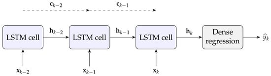
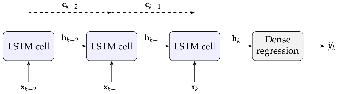
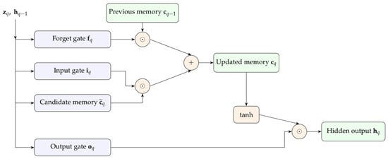
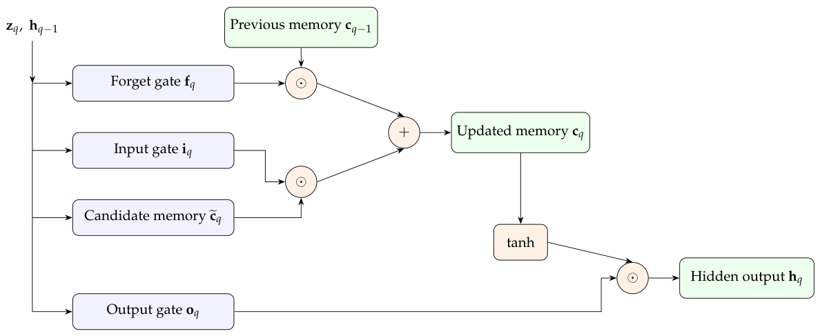
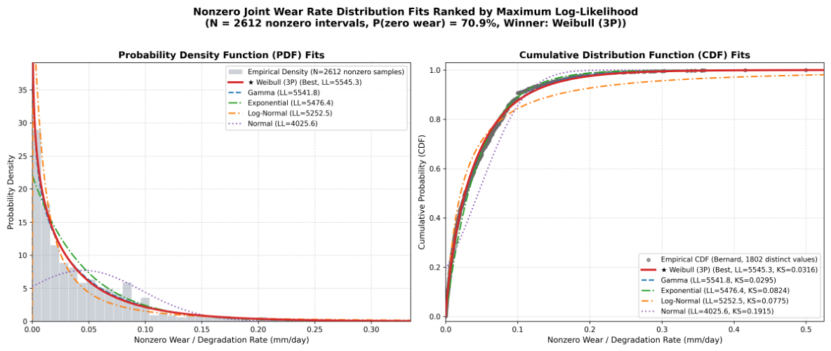
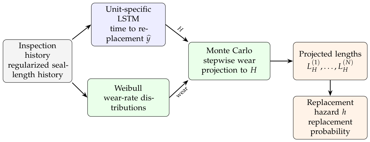
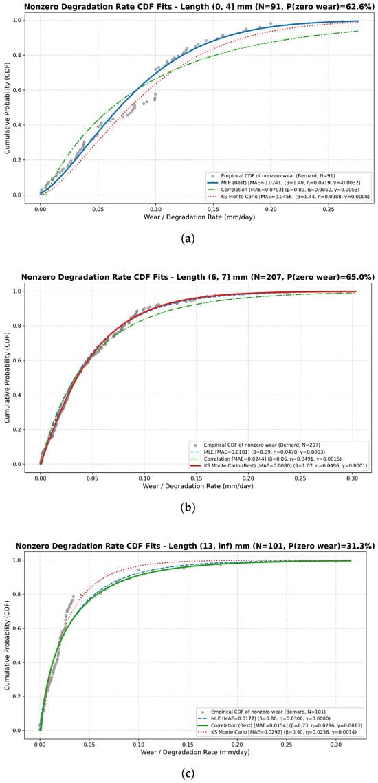
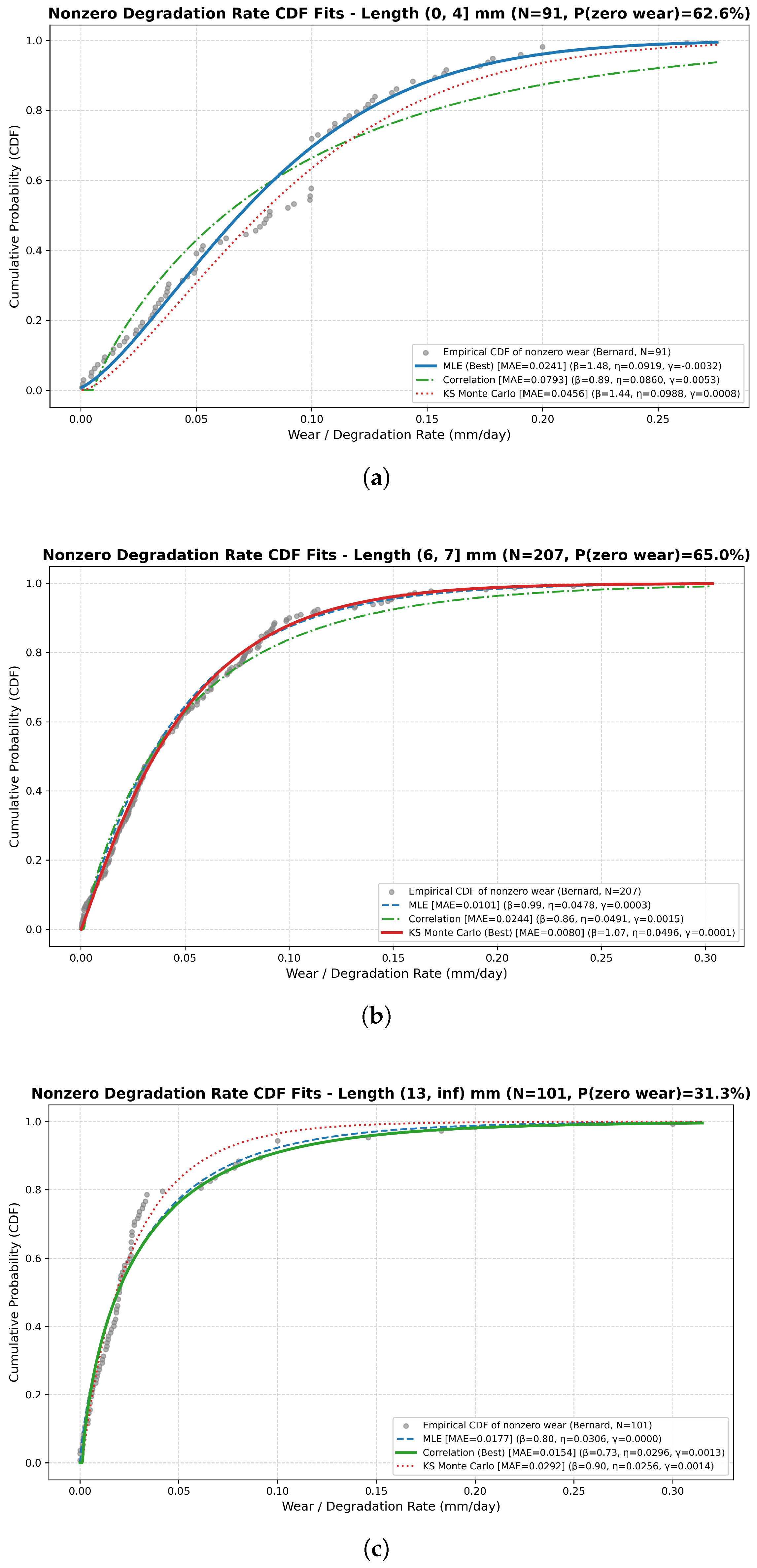
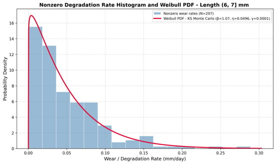
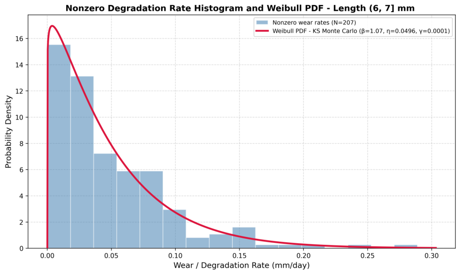
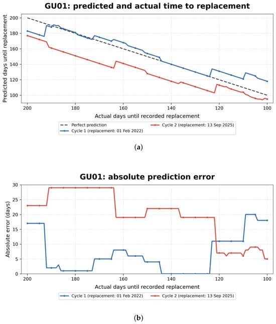
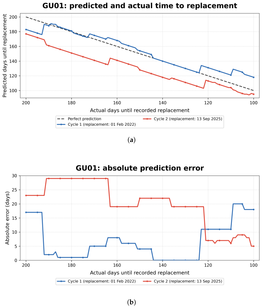
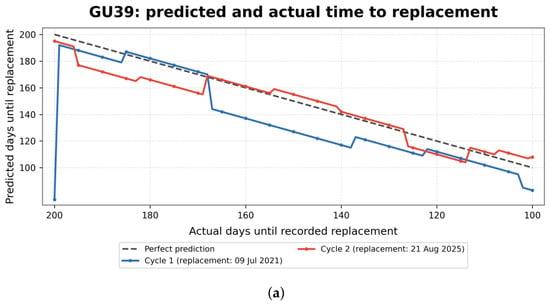
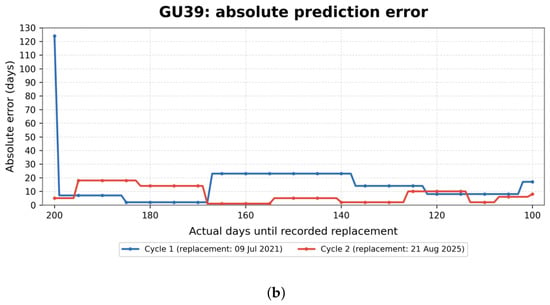
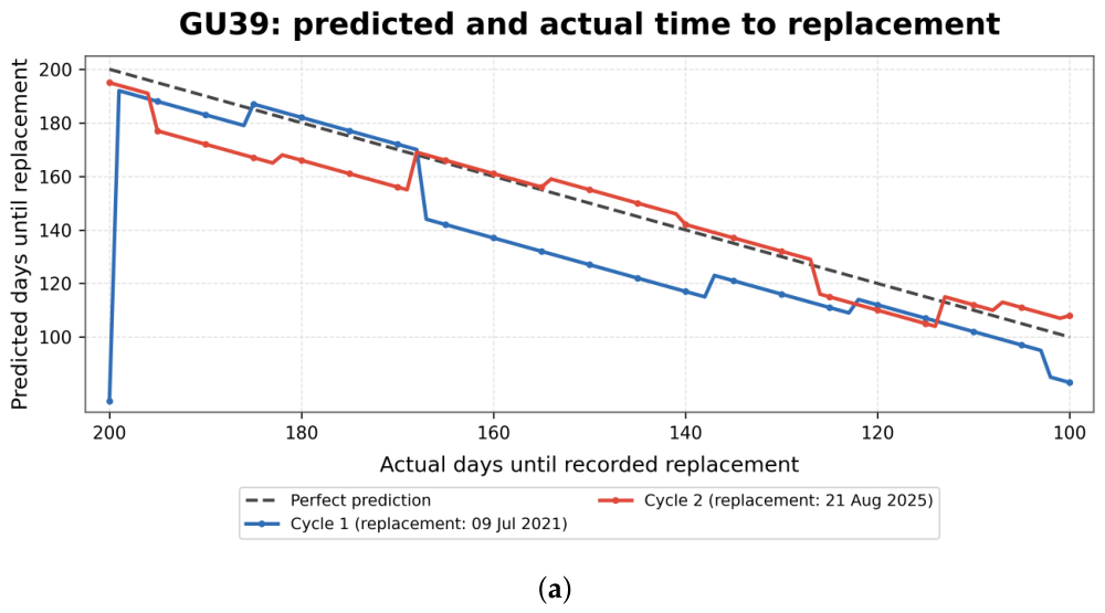
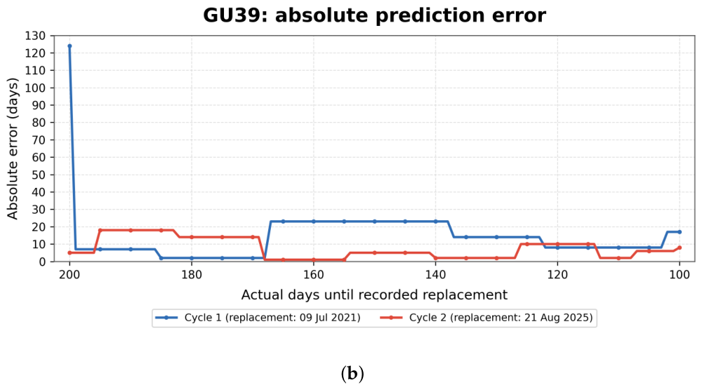
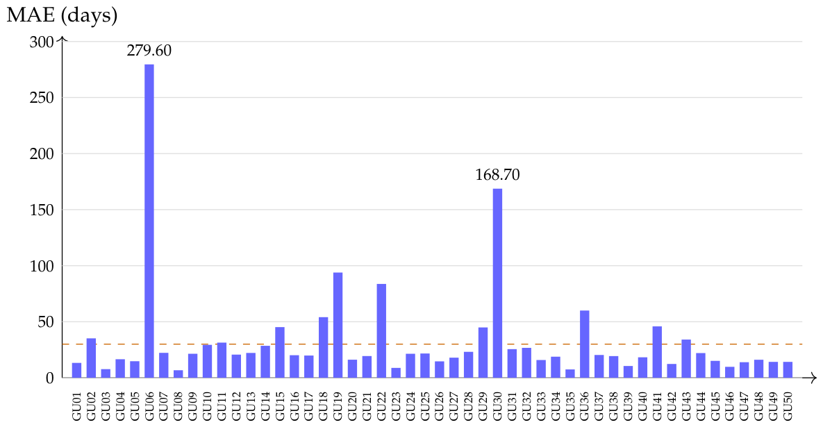
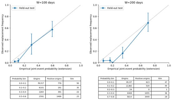
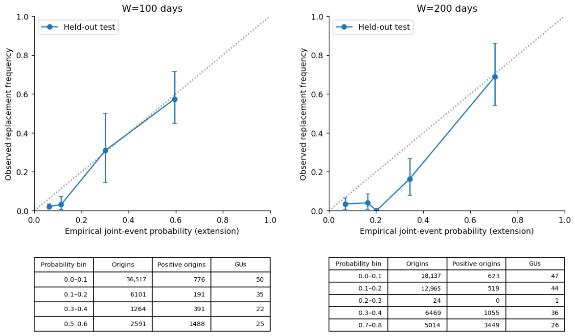

Disclaimer/Publisher’s Note: The statements, opinions and data contained in all publications are solely those of the individual author(s) and contributor(s) and not of MDPI and/or the editor(s). MDPI and/or the editor(s) disclaim responsibility for any injury to people or property resulting from any ideas, methods, instructions or products referred to in the content. |
© 2026 by the authors. Licensee MDPI, Basel, Switzerland. This article is an open access article distributed under the terms and conditions of the Creative Commons Attribution (CC BY) license.