


Abstract
Conservation voltage reduction (CVR) factors are usually estimated from field measurements by regressing load power on voltage. At the level of an individual industrial branch circuit, this regression is confounded, because a branch’s own current draw lowers its own bus voltage through simple Ohm’s-law feeder impedance. The naive coefficient then reflects reverse causation rather than the demand response to voltage that CVR programs are meant to quantify. This paper demonstrates the problem and tests a partial remedy using minute-resolution voltage (PT) and current/power (CT) data from 24 branch–hub pairings (23 analyzable) at three industrial facilities: a textile mill (SHIC), a metal heat-treatment plant (YC2), and a metal fabrication job shop (DSPM). All three sites are metered hierarchically, so every branch shares a common upstream (hub) bus, and the data span 63–90 days each across two non-overlapping calendar years. Naive ordinary least squares (OLS) regressions of log power on log branch voltage, with hour-of-day and day-of-week fixed effects and standard errors clustered by calendar day (residual autocorrelation remains above 0.68 at a 3 h lag, so conventional heteroskedasticity-robust errors are not adequate), produce CVR factors as extreme as −67, far outside the physically expected 0–2 range. Instrumenting each branch’s voltage with the site’s hub-bus voltage in a two-stage least squares (2SLS) design brings 5 of 13 severely biased branches within a credible magnitude bound (|β_IV| ≤ 2) across the three sites; all five, however, retain a negative sign that is physically anomalous for a passive load, so none become plausible by the strict 0-to-2 definition used throughout this paper. Properly clustered inference shows this magnitude-bound result is also precisely estimated, i.e., reliably distinguishable from zero, for only two of the five. The branches that reach the magnitude bound track each site’s hub-bus exogeneity rather than any branch-level property. At the one site with a near-exogenous hub (YC2, r = −0.07 between hub voltage and total site power), three of three severely biased branches have their magnitude brought within bound, though none precisely and all remain negative-signed. At the two sites with a substantially endogenous hub (SHIC, r = −0.57; DSPM, r = −0.71, using a same-facility proxy bus after its designated main proved unusable because its logged period did not overlap the rest of the site’s instrumentation), only 1 of 5 branches at each site has its magnitude brought within bounds, precisely (t < −6 in both cases) but still negative-signed. The same low magnitude-bounding rate recurs at a third site in a different calendar year; with only three site-level observations, we treat this as an exploratory extension of the pattern rather than an independent statistical replication. A further robustness check instruments YC2 with a second, more upstream measurement point. It fails outright: the cluster-robust first-stage F falls to 0.005–0.89 for every branch, against 3.5 × 10³–2.1 × 10⁶ for the hub used in the main design. The reason is that this alternative point sits on the far more tightly regulated side of the site’s service transformer (voltage SD ≈ 0.5% of mean) and shares little variation with the internally generated fluctuations (SD ≈ 3%) it would need to instrument. A valid instrument must share the endogenous variable’s own variation; sitting further upstream is not enough. The method requires no logged transformer tap-change event, unlike existing measurement-based CVR practice, and uses only the hierarchical metering structure already present in many industrial submetering deployments. Its contribution, however, is to bound the magnitude of a severe bias, not to restore full physical plausibility: without a ground-truth benchmark, we cannot claim the shifted estimates are closer to the true CVR factor, only that their magnitude changed and, in five of 13 cases, moved within a credible bound. The result is partial, site-conditional, persistently wrong-signed, and in most cases imprecise.
1. Introduction
Conservation voltage reduction (CVR) lowers a distribution feeder’s operating voltage, within the allowed service range, to reduce the active power drawn by voltage-sensitive loads and the associated energy consumption and peak demand [1,2]. The technique requires no new generation or storage and has been implemented at utility scale for decades [1]. However, quantifying how much power a given feeder or facility will actually save at a given voltage reduction still depends on the composition of the connected load, which varies by feeder, by facility, and by time of day [2]. This quantity is the CVR factor: the percentage change in power per percentage change in voltage. For industrial facilities specifically, a recent comprehensive review of CVR research identifies the response of industrial and composite commercial/industrial loads as one of the technology’s persistently unclear technical aspects, alongside the practical difficulty of obtaining a reliable, facility-specific load model [3].
Two broad families of methods are used to estimate a CVR factor from field measurement rather than from a bottom-up appliance model. The first instruments an actual voltage change, most directly a transformer load-tap-changer (OLTC) tap operation, and compares load immediately before and after it. A recent method demonstrated on the Korean utility KEPCO’s system estimates CVR factors directly from the voltage and load changes that occur at the moment of a naturally occurring tap change, without requiring an intentional test change [4]. The second regresses power on voltage over an extended measurement period, typically within a ZIP (constant-impedance, constant-current, constant-power) load-model framework. This approach has been made robust to time-varying load composition and measurement noise using recursive least squares with a variable forgetting factor and outlier-robust weighting, applied to substation-level phasor measurement unit (PMU) data [5]. A separate strand of this regression-based literature estimates ZIP coefficients and CVR factors for individual residential appliances under a controlled, intentionally varied supply voltage [6].
Both existing families depend on something that is often unavailable at the level of an individual industrial facility’s internal branch circuits. The tap-change method [4] requires a logged OLTC operation. Many industrial submetering deployments, including all three facilities studied here, record potential-transformer (PT) and current-transformer (CT) measurements continuously but do not log any voltage-regulation event at all. The regression-based methods [5,6] treat voltage as if it varies independently of the load whose response is being estimated. This is a defensible approximation at a substation fed by a wide-area transmission system weakly loaded by any single feeder, but not at an individual branch circuit a few tens of meters from the metered bus, whose current directly produces the voltage drop being regressed against. On such a branch, a load increase at time t simultaneously raises P(t) and, through the feeder’s own impedance, lowers V(t). A regression of P on V estimated this way conflates the demand response to voltage that a CVR program is meant to quantify with this reverse, Ohm’s-law channel running from load to voltage. This is a standard endogeneity problem, but to our knowledge it has not been demonstrated or corrected using real, multi-point, hierarchically metered industrial branch-circuit data. Nor has it been exploited as an opportunity: the same metering hierarchy that creates the problem at the branch level also supplies, at every site with more than one metered branch, a natural candidate instrument, the voltage at the common bus every branch shares upstream. That common bus depends on any single branch’s current only weakly, since the current is diluted by every other branch sharing the same bus.
The contributions of this study are to:
- Demonstrate the branch-level endogeneity problem empirically, using minute-resolution PT/CT data from 24 branch–circuit pairings at three real industrial facilities. Naive OLS regression of log power on log voltage produces CVR factors as extreme as −67, more than thirty times the physically expected magnitude, once standard errors are clustered by calendar day to account for residual autocorrelation too persistent for conventional heteroskedasticity-robust errors alone.
- Propose and implement a common-bus instrumental-variable (IV) correction, via two-stage least squares (2SLS), that requires only the metering hierarchy already present at each site and no logged tap-change event.
- Show that the correction brings 5 of 13 severely biased branches within a credible magnitude bound (|β_IV| ≤ 2), though all five remain negative-signed and therefore outside the strict physically plausible range; only 2 of the 5 are also statistically distinguishable from zero once inference accounts for serial correlation. A site-level property of the shared hub bus, how strongly its own voltage already co-varies with the site’s own total demand, separates branches whose magnitude is brought within bound from those that are not.
- Show that the standard first-stage F-statistic correctly flags the one structurally degenerate instrument pairing tested, but remains large for every other pairing regardless of whether the magnitude bound is reached. We propose a complementary site-level exogeneity screen for this reason.
- Test a robustness check that instruments with an alternative, more upstream measurement point, which fails for every branch tested. This refines the design principle for choosing a common-bus instrument: proximity to the grid is not sufficient, and the instrument must carry enough of the same variation as the branches it instruments.
- Show that a third site, whose designated main bus could not be used at all because its logged period did not overlap the rest of the site’s instrumentation, shows the same low magnitude-bounding-rate pattern found at the first high-endogeneity site, using an ordinary sibling bus as a substitute instrument. With only three site-level observations, we treat this as an exploratory extension of the pattern from two sites to three, not as an independent statistical replication, and it shows that the diagnostic still functions when a facility’s true point of common coupling is unusable.
Taken together, these contributions give industrial CVR assessment a diagnostic method: a way to test, rather than assume, whether a given multi-point metering deployment supports a valid branch-level voltage-power sensitivity estimate.
2. Related Work
Measurement-based CVR estimation. The foundational utility-scale CVR demonstrations [1,2] established the empirical practice of comparing feeder load before and after a deliberate or naturally occurring voltage-regulation event. Building on this, ref. [4] proposed a direct method and a mean-absolute-deviation-adjusted direct method to estimate active- and reactive-power CVR factors from KEPCO distribution data at the moment of an OLTC tap change, explicitly avoiding the need for an intentionally scheduled test. This remains, to our knowledge, the closest prior measurement-based approach to the setting of the present paper. It is also the approach whose data requirement, a logged tap event, our method is designed to avoid.
Regression- and load-model-based CVR estimation. Where no discrete voltage event is available, CVR factors are more commonly estimated within a ZIP load-model framework by regressing power on voltage over a continuous measurement window. Reference [5] develops a robust recursive least-squares estimator with a variable forgetting factor and a Huber M-estimator to track time-varying ZIP parameters from noisy, possibly gap-ridden PMU data at substation scale. Reference [6] estimates ZIP coefficients and CVR factors for individual residential appliances and an aggregated residential feeder under a controlled, intentionally stepped supply voltage. Neither treats voltage as a variable that the regression’s own dependent variable can feed back into. That is a reasonable simplification at a substation or under laboratory voltage control, but not, as Section 4.2 shows, at an industrial branch circuit under normal operation.
Endogeneity and instrumental variables. The reverse-causation problem this paper addresses is a textbook case of regressor endogeneity: a regressor (voltage) is itself partly determined by the outcome it is used to explain (power), through a channel (feeder impedance) outside the regression. Econometrics standardly addresses this with instrumental variables and two-stage least squares [7,8]. A valid instrument must be correlated with the endogenous regressor (relevance) but uncorrelated with the regression’s error term through any channel other than that regressor (the exclusion restriction), and the strength of the first stage is routinely screened with an F-statistic against a critical value derived for typical econometric sample sizes [9]. We are not aware of a prior application of this framework to branch-level, field-measured CVR factor estimation. The contribution here is to show both that the underlying metering hierarchy of a multi-branch industrial facility supplies a natural candidate instrument, and that its validity must be checked at the site level rather than assumed from a large first-stage F-statistic alone.
Instrumental variables in energy economics. Outside power-systems engineering, IV designs routinely isolate a genuine response from confounded field data, for example, the effect of feed-in tariffs on renewable generation [10], the household-level impact of rural electrification [11], smart-meter feedback as a natural experiment [12], price elasticity under high-frequency autocorrelation [13], and demand response under instrumented price variation [14]. All share our identification logic: variation plausibly unrelated to the unit’s own shock. None, to our knowledge, use it for voltage as the endogenous regressor of an individual metered load.
Load modeling beyond the substation aggregate. ZIP coefficients have been determined experimentally for modern loads [15], compared against an exponential alternative for CVR evaluation [16], estimated with a Bayesian approach [17], and determined per-appliance in a smart-home testbed [18]. All of this work operates at the level of an appliance or a laboratory feeder, where voltage can be varied independently of the load under test, a condition an industrial branch circuit under normal operation does not satisfy.
Voltage control and distributed energy resources. Both SHIC and YC2 operate OLTC and SVG equipment, though neither logs tap or reactive-power events for this study (Section 5.3). This connects the analysis to work on joint CVR/Volt-VAR optimization [19], OLTC control under rising renewable penetration [20], and reinforcement-learning Volt-VAR control [21]. On-site generation and storage further complicate CVR delivery and its measurement. Related work covers feeder-voltage design for PV hosting capacity [22], direct analysis of PV’s interaction with CVR effectiveness [23], and battery storage for voltage regulation [24] and multi-service ancillary support [25]. This literature is why YC2’s photovoltaic branch (A03) is treated separately from conventional loads in Section 4.2.
Industrial submetering and load characterization. Continuous PT/CT measurement at branch-circuit level is increasingly common, but it has mostly been studied for purposes other than CVR. Industrial non-intrusive load monitoring remains less mature than its residential counterpart [26]. Embedded sensor networks [27] and deployed monitoring systems [28] target energy efficiency, and industrial power quality has been assessed with low-cost [29] and high-resolution [30] instrumentation. Where PMUs are available, load composition can be estimated at higher rates [31], trading resolution for the broader deployment that the one-minute PT/CT setting used here already offers. Smart-meter measurements have similarly been used to identify distribution-network topology and line impedance [32,33]. Our contribution is to show that this same hierarchical structure can also support CVR-factor identification.
Graph neural networks for network-structured causal inference. Beyond power-system applications, a growing literature uses graph neural networks (GNNs) to address hidden confounding and interference in networked observational data. This includes adjusting for network confounding when covariates and topology jointly drive selection bias [34], estimating causal effects under general network interference and intervention [35], and learning invariant graph representations to isolate a causal effect from a spurious network correlation [36]. A different methodological tradition, classical spatial econometrics, instruments a spatially lagged endogenous variable with neighboring units’ characteristics [37]. Section 5.4 discusses how these ideas could extend the present paper’s single-instrument design to a network-structured one, using the electrical coupling between branches that Section 3.4 currently treats only as a nuisance.
3. Materials and Methods
3.1. Site Description and Data Acquisition
Data were collected from three industrial facilities, denoted SHIC (a textile mill), YC2 (a metal heat-treatment plant), and DSPM (a metal fabrication job shop centered on laser cutting), each instrumented with potential transformers (PT, one per metered bus, reporting per-phase and average line-to-line voltage) and current transformers (CT, one or more per bus, reporting per-phase current and active/reactive power) at one-minute resolution. All three sites are metered hierarchically: every branch bus is fed, directly or through intermediate switchgear, from a single site-wide hub bus at the point of utility interconnection, so every branch’s voltage and the hub bus’s voltage are electrically coupled through the same upstream service transformer and conductors. SHIC and YC2 were logged over the same 90-day window (1 January 2026 to 1 April 2026); DSPM was logged independently over a 90-day window one calendar year earlier (1 January 2025 to 31 March 2025, plus a separate, non-overlapping 10-day log for one bus discussed below), so the cross-site comparison in Section 4 spans two non-overlapping periods, not only three facilities.
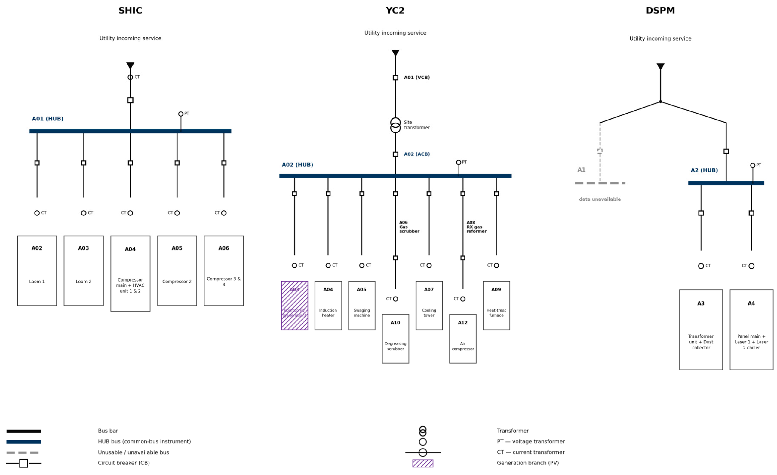
SHIC’s hub bus (A01) directly aggregates the site’s main incoming feed. Five further buses (A02–A06) each carry their own dedicated PT and one to three CT channels serving individual loom, compressor, and HVAC circuits. YC2 distinguishes two upstream measurement points: a vacuum circuit breaker (VCB) bus (A01) and, downstream of the site transformer, an air circuit breaker (ACB) bus (A02). Ten further buses (A03–A12) meter individual process loads (induction heating, swaging, degreasing, heat treatment, and a rooftop photovoltaic interconnect at A03) plus one air compressor. A11 is also instrumented but is not included in this paper’s branch-level analysis in Section 4. We treat A02 (ACB) as each site’s common hub bus for the instrumental-variable design in Section 3.4, since it is the point common to every downstream branch. A01 (VCB) is retained as a branch in its own right, providing an internal validity check (Section 4.3).
DSPM’s device list designates A1 as its main bus, but A1’s own PT log covers only 1 April 2025 to 10 April, a window that overlaps none of the site’s other instrumentation, including A1’s own CT children, which are logged 1 January 2025 to 31 March 2025 like the rest of the site. Even A1’s branch-level regression cannot be estimated as a result. We therefore instrument the remaining branches (A3, A4) with A2 instead. Among the three buses with usable overlapping data, A2 has the weakest (least negative) correlation with the site’s total metered power (r = −0.71, versus −0.76 for A3 and −0.91 for A4), making it the least contaminated available substitute for the unusable main bus. A2 is an ordinary sibling bus rather than a validated point of common coupling, so DSPM’s results in Section 4 test the method under a realistically imperfect hub choice rather than the idealized design of Section 3.4.
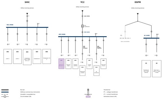
Figure 1 shows simplified single-line diagrams of each site’s metering hierarchy, marking the hub bus used as the common-bus instrument, every branch bus, and the PT/CT measurement location at each. For YC2, the diagram places the site service transformer explicitly between A01 (VCB) and A02 (ACB) to show that these are two measurement points on either side of one transformer, not independent buses; this is the physical basis for the diagnostic results of Section 4.3 and Section 4.5. For DSPM, the diagram marks A1 as unusable, with its non-overlapping logging period noted, and A2 as the substitute hub actually used in its place (Section 3.1). This figure is a schematic representation of the metering hierarchy described above and in Table 1, constructed from the site’s device-mapping records and the relationships stated in this section; it is not a reproduction of the facilities’ own as-built electrical single-line drawings, which were not available to us in digital form.
Figure 1.
Schematic representation of each site’s metering hierarchy (not an as-built electrical drawing), showing the hub bus used as the common-bus instrument, branch buses, and PT/CT measurement locations, constructed from the site description in Section 3.1 and the device-mapping records.
Table 1.
Site and dataset summary.
3.2. Data Preprocessing
For each PT/CT pairing sharing a bus, active power (P), reactive power (Q), and average line-to-line voltage (V) were merged on a common one-minute timestamp index over each site’s full measurement period. Timestamps with non-positive active power (idle or sign-convention artifacts, predominantly overnight at intermittently used branches) or line-to-line voltage below 100 V were dropped prior to estimation; the latter condition indicates a sensor fault or de-energized bus, and one YC2 branch that reads a near-constant ~0.00003 V throughout is excluded on this basis. DSPM’s A4 bus reads a plausible but markedly lower line-to-line voltage (≈212 V, versus 370–390 V at every other bus across all three sites). This is consistent with a separately regulated or lower-voltage-class tap rather than a sensor fault, since it fluctuates coherently with A4’s own load (Section 4.4), and it is retained because the log-log specification below identifies a relative, not absolute, voltage–power relationship. Two calendar features, hour-of-day (0–23) and day-of-week (0–6), were retained as categorical fixed effects.
3.3. Naive OLS Specification
For branch i with voltage V_i(t) and active power P_i(t), the conventional log-log CVR factor regression is
where D_hour and D_dow are hour-of-day and day-of-week dummy vectors, and β_OLS is the estimated CVR factor for active power (the elasticity of P with respect to V). An initial heteroskedasticity-robust (HC1) pass is used only to diagnose the severity of serial correlation in the naive specification; every coefficient reported as a result in this paper, here and throughout, instead uses the calendar-day clustered standard errors described in Section 3.5. Textbook ZIP-model CVR factors for real power fall between 0 (pure constant-power load, no sensitivity to voltage) and 2 (pure constant-impedance load). We define the physically plausible range as 0 ≤ β ≤ 2: both the sign and the magnitude must be correct. An estimate with |β| ≤ 2 but a negative sign is not plausible by this definition; we call it magnitude-bounded, and distinguish the two terms consistently throughout (Section 3.4).
ln P_i(t) = α + β_OLS ln V_i(t) + γ′ D_hour(t) + δ′ D_dow(t) + ε(t)
3.4. The Endogeneity Problem and a Common-Bus Instrumental Variable
At an individual branch circuit, V_i(t) is not exogenous to ε(t). The same current that produces P_i(t) also produces a voltage drop across the branch’s own feeder impedance, so an unobserved shock that raises P_i(t) (e.g., an additional motor starting) mechanically lowers V_i(t) at the same instant. This biases the OLS estimate β_OLS away from the true demand response, potentially by a very large factor, as Section 4.2 shows. Algorithm 1 summarizes the resulting correction procedure, including the diagnostics of Section 3.5 and Section 5.1 that decide whether a given branch–hub pairing may be trusted.
| Algorithm 1. Common-Bus Instrumental-Variable Correction for a Branch CVR Factor |
| Input: branch series V_i(t), P_i(t); hub series V_main(t); calendar dummies D_hour(t), D_dow(t) Output: IV-estimated CVR factor β_IV, clustered SE, first-stage F, plausibility flag, hub-exogeneity diagnostic r_hub 1: Merge V_i, P_i, V_main on timestamp t; drop P_i(t) ≤ 0 or V(t) < 100 V; 2: Fit first stage: ln V_i(t) = π0 + π1 ln V_main(t) + γ′D_hour + δ′D_dow + u(t); 3: F ← cluster-robust F-statistic on π1 (clusters = calendar day); 4: if F < 10 then 5: flag pairing INVALID INSTRUMENT; return ∅; 6: end if 7: V̂_i(t) ← fitted values from Step 2; 8: Fit second stage: ln P_i(t) = α + β_IV ln V̂_i(t) + γ′D_hour + δ′D_dow + ε(t), with SE clustered by calendar day; //via a joint IV2SLS estimator (Section 3.5); SE reflects first-stage estimation uncertainty, not a naive plug-in-OLS SE 9: if 0 ≤ β_IV ≤ 2 then 10: flag PLAUSIBLE; 11: else if |β_IV| ≤ 2 then 12: flag MAGNITUDE-BOUNDED, WRONG SIGN; 13: else 14: flag UNCORRECTED; 15: end if 16: r_hub ← corr(V_main(t), P_main(t)); //site-level exogeneity screen, reported alongside flag (Section 5.1), not used as a pass/fail gate 17: return β_IV, SE, F, flag, r_hub. |
We address this with a standard two-stage least squares (2SLS) design, instrumenting each branch’s voltage with the site’s hub-bus voltage V_main(t):
First stage: ln V_i(t) = π0 + π1 ln V_main(t) + γ′ D_hour(t) + δ′ D_dow(t) + u(t)
Second stage: ln P_i(t) = α + β_IV ln V_fit,i(t) + γ′ D_hour(t) + δ′ D_dow(t) + ε(t), where V_fit,i(t) is the first stage’s fitted value
The identifying logic is that V_main(t) is correlated with V_i(t), because both are drawn down by the same upstream transformer and service impedance (relevance). Any single branch i’s own current, however, is only one of many contributors to V_main(t), diluted by every other branch sharing the same hub. V_main(t) is therefore plausibly much less directly driven by branch i’s own idiosyncratic load shock than V_i(t) is (exclusion restriction). This exclusion restriction is an approximation rather than an identity, and Section 4.3 and Section 4.4 examine its validity empirically rather than assume it.
3.5. Estimation Protocol and Diagnostics
One-minute field data of this kind are strongly serially correlated. For a representative branch, the residual autocorrelation of the naive specification is 0.99 at a 1 min lag and still 0.85 and 0.68 at 1 h and 3 h lags, respectively, far beyond what a fixed-lag Newey–West window can practically span. We therefore report cluster-robust standard errors with calendar day as the cluster (79–90 clusters per branch, depending on data coverage), which allows arbitrary within-day correlation while treating days as the approximately independent unit. Conventional heteroskedasticity-robust (HC1) errors, used only for the exploratory pass that motivated this design, understate the true sampling uncertainty by an order of magnitude or more at this autocorrelation level. Both stages were estimated jointly by a formal two-stage least squares estimator (Python 3.12; linearmodels v7.0 IV2SLS, cross-checked against statsmodels v0.14.6 first-stage OLS; pandas v3.0.5 for data handling) for every branch–hub pairing with at least 2000 valid observations, excluding the pairing’s own hub bus from the set of source branches. The reported second-stage standard errors come from this joint estimator’s cluster-robust covariance, which propagates first-stage sampling uncertainty into the second stage; they are not computed by running an ordinary OLS regression of the second stage on the first stage’s fitted values alone, which would understate the true standard error by ignoring that additional source of variation. Three diagnostics accompany every estimate. The first is the cluster-robust partial first-stage F-statistic (equivalently, the squared cluster-robust t-statistic) on the excluded instrument, screened against the conventional critical value of 10 [9]. The second is the branch’s load share, its mean active power as a fraction of the hub bus’s mean active power, used as a proxy for how much a branch’s own current could plausibly contribute to hub-bus voltage and thus violate the exclusion restriction. The third is statistical significance of β_IV itself (|t| > 1.96), since a point estimate inside the credible-magnitude bound is not informative if its confidence interval is very wide. Section 4.3, Section 4.4 and Section 4.5 show that none of these, alone, fully explains which branches reach the magnitude bound; Section 4.5 adds a robustness check that instruments with a second, alternative hub at YC2.
The PT/CT hardware used at all three sites (Rootech ACCURA 2300S for voltage, ACCURA 2350-3P for current; Rootech Inc., Suwon, Republic of Korea) is rated at ±0.2% of reading for both voltage and current, and IEC 61557-12 Class 0.5 for active power. The measured line-to-line voltage standard deviation is several times larger than this accuracy band (≈0.9% of the mean at SHIC’s hub, ≈3% at YC2’s), so instrument noise is unlikely to be the dominant source of the OLS bias reported in Section 4.2. It cannot, however, be ruled out as a contributor to the near-zero, low-precision estimates discussed in Section 4.4.
4. Results
4.1. Site-Level Voltage–Load Coupling
Before turning to branch-level estimates, we characterize each site’s hub bus (or, for DSPM, its best-available substitute; Section 3.1). Section 4.4 shows that this characterization anticipates where the instrumental-variable correction will and will not work. Over each site’s full study period, the Pearson correlation between the hub bus’s own voltage and its own total active power is r = −0.57 at SHIC, r = −0.07 at YC2, and r = −0.71 at DSPM (all p < 0.001; n > 110,000 at SHIC/YC2, n ≈ 126,000 at DSPM). The SHIC and DSPM hub buses are materially more coupled to their own site’s aggregate demand than YC2 is. Weekly operating rhythm differs correspondingly. SHIC runs close to continuously (mean active power on Saturday/Sunday is 97%/98% of the Monday–Friday mean). YC2 follows a conventional five-day schedule (51% and 31% of the weekday mean). DSPM’s job-shop laser-cutting operation is the most variable of the three, plausibly consistent with the strongest self-generated share of its own hub-bus voltage variation.
4.2. Naive OLS CVR Factors Are Frequently Implausible
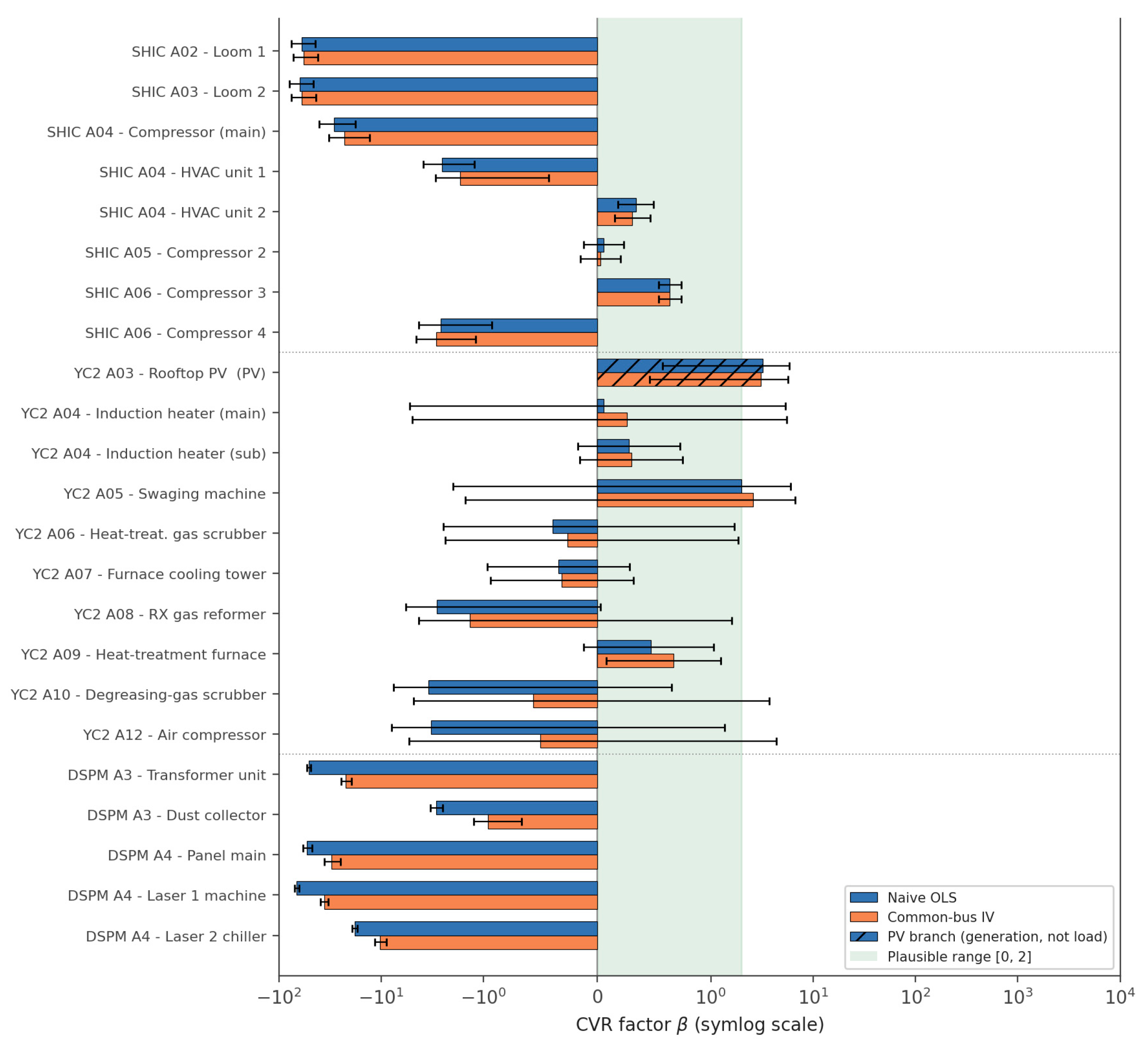
Table 2 reports the naive OLS and IV-corrected CVR factor for every branch–hub pairing across all three sites. Of 24 pairings tested, one (YC2 A01, the VCB bus) is excluded from interpretation because its instrument is structurally degenerate (Section 4.3), and one (YC2 A03, the rooftop photovoltaic interconnect) reflects generation-side physics rather than a load CVR factor and is reported separately. Of the remaining 22 load branches, naive OLS places 7 within the physically plausible range 0 ≤ β ≤ 2 (SHIC’s A04 HVAC unit 2, A05 Compressor 2, and A06 Compressor 3; YC2’s A04 induction heater main and sub, A05 swaging machine, and A09 heat-treatment furnace). Two further branches, YC2’s A06 heat-treatment gas scrubber (−0.39) and A07 furnace cooling tower (−0.34), have a naive-OLS magnitude within the credible bound but a negative sign; we report these separately rather than as plausible, since bounded magnitude alone does not establish plausibility (Section 3.3). The remaining 13 branches are severely biased in magnitude under naive OLS, from −2.55 to as extreme as −67 at DSPM’s Laser 1 machine branch (A4), narrowly beyond the two SHIC loom branches (A02, A03) and the SHIC compressor-main branch (A04). All 13 are more than an order of magnitude beyond the plausible range, and every one of DSPM’s five tested branches falls in this severely biased group.
Table 2.
Naive OLS and common-bus IV-corrected CVR factor for active power, by branch. Standard errors clustered by calendar day, in parentheses. Bold marks branches with |β| > 2, the credible-magnitude bound; this flags magnitude only, not sign (Section 3.3).
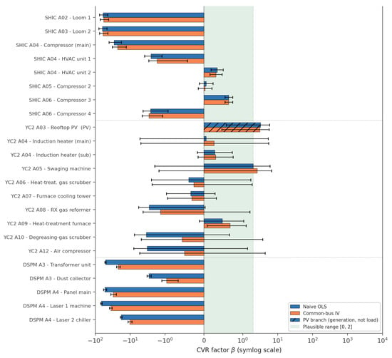
Figure 2 plots the naive and IV-corrected point estimates on a symmetric-log scale with 95% confidence intervals from the day-clustered standard errors, shaded to mark the physically plausible range 0 to 2. The correction reduces the magnitude of every severely biased branch’s point estimate, but only rarely brings it fully inside that range, since most of the magnitude-bounded estimates remain negative in sign.
Figure 2.
CVR factor by branch, naive OLS vs. common-bus IV (symlog scale; error bars: 95% CI). Shaded band = physically plausible range [0, 2] (Section 3.3); several IV estimates fall below zero and are therefore outside this band despite being brought within |β| ≤ 2.
4.3. Instrument Diagnostics: A Genuinely Invalid Pairing and a Misleadingly Reassuring F-Statistic
YC2’s A01 (VCB) bus is excluded from Table 2’s interpretation because its instrumented estimate is not credible: β_IV = −1743 (clustered SE = 6282), three orders of magnitude beyond every other estimate. Its cluster-robust first-stage F is 0.07, far below the conventional weak-instrument threshold of 10 [9], correctly flagging the problem. The cause is structural, and it is the same mechanism Section 4.5’s robustness check independently uncovers for the same two buses: A01 (VCB) sits on a comparatively stiff, tightly regulated part of the interconnection, with a voltage standard deviation of only about 0.5% of its mean, while A02 (ACB), on the other side of the same site service transformer, varies roughly six times more (≈3%). A01 simply does not move enough to explain A02’s much larger, locally generated voltage swings, so the first stage is weak rather than merely imprecise. This is not the near-collinearity failure that “two metering points on the same transformer” might suggest; near-collinearity would instead produce a spuriously strong, not a weak, first stage. It is a relevance failure, consistent with the direct variance comparison Section 4.5 reports for these same two buses. This is a useful negative result in its own right: a metering hierarchy with only two upstream measurement points on the same transformer does not automatically supply a usable instrument for this design, and the diagnostic correctly flags it, for the reason Section 4.5 confirms directly.
For every one of the remaining 23 pairings across all three sites, the cluster-robust first-stage F is still large, from 1.4 × 10³ to 2.1 × 10⁶, regardless of whether the corresponding IV estimate in Table 2 is physically plausible or precisely estimated. Properly clustering the standard errors (Section 3.5) brings these values down by several orders of magnitude from a naive HC1 calculation, but they remain well above the weak-instrument threshold for every pairing except A01. The first-stage F-statistic can therefore rule out a genuinely degenerate instrument, as it did for A01, but it says nothing about whether the second-stage estimate it supports is precisely estimated or economically plausible. Different diagnostics, developed in Section 4.4 and Section 4.5, are needed for that.
4.4. Where the Magnitude Bound Is Reached, and Why Precision Differs Across Branches
Among the 13 branches severely biased under naive OLS (excluding A01), the common-bus IV correction brings 5 point estimates within the credible-magnitude bound |β_IV| ≤ 2: YC2’s degreasing-gas scrubber (A10, −3.44 → −0.56), air compressor (A12, −3.26 → −0.50), and RX gas reformer (A08, −2.85 → −1.35); SHIC’s HVAC unit 1 (A04, −2.55 → −1.68); and DSPM’s dust collector (A3, −2.90 → −0.96). Every one of these five estimates is negative, so none of them actually falls inside the physically plausible range 0 ≤ β ≤ 2 defined in Section 3.3: the correction reduces the magnitude of a severe bias without restoring the physically expected sign, and we do not describe any of the five as plausible. Under day-clustered inference, SHIC’s HVAC unit 1 (t = −2.63) and DSPM’s dust collector (t = −6.39) are precisely estimated, meaning their confidence intervals reliably exclude zero; this is a statement about estimation precision, not about physical plausibility—a negative coefficient estimated precisely is still a negative, physically anomalous coefficient. The three YC2 corrections have |t| < 1.0 (RX reformer −0.90, scrubber −0.26, compressor −0.20); their confidence intervals span most of the credible-magnitude band and beyond, and do not exclude either zero or the original OLS estimate. The remaining 8 severely biased branches, both SHIC looms (A02, A03), SHIC’s compressor-main and A06 COMP#4, and all four other DSPM branches (A3 transformer unit; A4 panel main, Laser 1 machine, Laser 2 chiller), stay beyond the credible-magnitude bound and remain strongly significant (|t| ≥ 3.0 at SHIC, |t| > 11 at every DSPM branch). Both sites’ uncorrected estimates are confidently wrong rather than merely noisy. The looms and DSPM’s transformer unit barely move at all (SHIC: −59.98 → −56.89 and −62.67 → −59.69, both |t| > 7; DSPM: −51.22 → −22.12, |t| > 16).
This site pattern is not confined to the branches that started out implausible. Across every load branch at YC2 (excluding the invalid A01 pairing and the generation branch A03), not one naive OLS coefficient is significant at the 5% level; the closest, RX reformer, has t = −1.94. At SHIC, 7 of 8 are significant regardless of whether the point estimate is plausible. At DSPM, all 5 tested branches are significant (|t| ≥ 6.4, naive OLS |t| > 13 in every case). We initially suspected that fewer complete calendar-day clusters at several YC2 branches (26–66 days of usable data, versus 79–87 at SHIC, reflecting YC2’s greater missing-data fraction) mechanically widened YC2’s clustered SEs. DSPM, however, has fewer usable days than SHIC (62–63) yet produces the most confidently estimated coefficients of any site, so day-count alone cannot be the main driver. The more likely explanation is first-stage relevance itself. Where a branch’s own voltage moves largely independently of the hub, as evidently happens for several YC2 branches, the first stage’s fitted values carry little variation, and 2SLS trades its magnitude shift for wider confidence intervals on exactly the branches where a good instrument matters most. SHIC’s and DSPM’s tested branches retain enough hub-explained variation to be estimated precisely, for better, in their one magnitude-bounded case each, or worse, in every branch that stays implausible.
We tested two further branch-level explanations for which point estimates reach the magnitude bound before returning to the site-level pattern. First, load share (Section 3.5) does not separate the outcomes. Across all three sites, computed as each branch’s mean active power over its own hub’s mean active power (Section 3.5), corrected branches range from 2.3% (SHIC’s HVAC unit 1) to 24.9% (DSPM’s dust collector), and uncorrected branches range from 7.2% (SHIC’s Loom 2) to 174% (DSPM’s Panel main, whose own mean load exceeds that of A2, the substitute hub it is referenced to): heavily overlapping ranges, not a clean threshold. Second, whether a branch is the sole load on its own dedicated PT/CT pairing, as both SHIC looms and every DSPM branch are, versus sharing a bus with siblings, does not separate them either. YC2’s corrected degreasing scrubber and compressor are each the sole CT child of their own bank, exactly like the uncorrected SHIC looms and every DSPM branch, whether corrected or not.
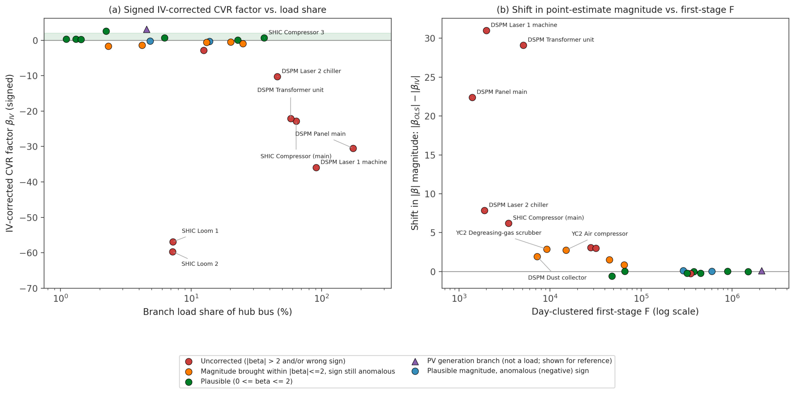
What separate the point-estimate outcomes is site membership. Of SHIC’s five severely biased branches, only one has its magnitude brought within bounds (20%); of YC2’s three, all three do (100%, though none precisely, and all remain negative-signed); of DSPM’s five, only one does (20%, precisely, and it too remains negative-signed). This tracks the hub-bus exogeneity gradient of Section 4.1. SHIC’s and DSPM’s hub buses are themselves strongly coupled to their own site’s total demand (r = −0.57 and −0.71, respectively), which is precisely the condition the exclusion restriction of Section 3.4 requires to be small. A contaminated hub shifts the point estimate persistently in a particular direction, and, because the contamination is systematic rather than random, does so with high apparent precision. SHIC’s and DSPM’s wrong answers are confident ones, and their one magnitude-bounded case at each site is also confidently estimated—confidently negative, not confidently plausible. YC2’s cleaner hub (r = −0.07) brings magnitude within bound more often but, as shown above, at the cost of precision, and still without achieving the correct sign. DSPM shows the same low-rate, high-confidence pattern as SHIC, at a different facility, using a different substitute instrument, in a different calendar year. This is exploratory rather than independently validated evidence: it rests on a third site-level observation, not a fourth independent one, and the branches within each site share that site’s hub and so cannot themselves supply additional independent support for a site-level relationship. It is, nonetheless, consistent with the pattern tracking the hub’s own exogeneity rather than an idiosyncrasy of one site or one time period. Figure 3 summarizes both diagnostics side by side.
Figure 3.
Instrument diagnostics. (a) Signed IV-corrected CVR factor vs. branch load share (sign retained; see Section 3.3). (b) Shift in point-estimate magnitude (|OLS| − |IV|) vs. day-clustered first-stage F (log scale); a large shift is not evidence of bias reduction without a ground-truth benchmark (Section 5.3). Only outlier branches are labeled by name (panel (a): |β_IV| > 5 or load share > 30%; panel (b): magnitude shift > 5 or first-stage F < 2 × 10⁴); unlabeled points are the remaining branches, whose values fall within this unremarkable range and can be identified individually in Table 2.
4.5. Robustness Check: Instrumenting with a Second, More Upstream Bus
A natural objection to Section 3.4’s design is that YC2’s A01 (VCB), sitting upstream of the site’s service transformer, should be an even better instrument than A02 (ACB): further diluted from any single branch’s own current, if dilution were all that mattered. We tested this directly, re-instrumenting A02 and every downstream branch (A03–A12) with A01 in place of A02. The result is unambiguous failure. The cluster-robust first-stage F falls to 0.005–0.89 for every branch tested, versus 3.5 × 10³–2.1 × 10⁶ for the same branches instrumented by A02, and the corresponding β_IV estimates become numerically meaningless (e.g., A03: −58.6; A10: −398; A12: −1009).
The reason is visible in the raw data rather than in any regression. A01’s line-to-line voltage has a standard deviation of about 1.9 V (≈0.5% of its mean), while A02’s is about 11.1 V (≈3%), nearly six times larger. A01 sits on a comparatively stiff, tightly regulated part of the interconnection and simply does not move enough to explain the much larger, locally generated voltage swings that A02 and every downstream branch share. Relevance (Section 3.4) requires the instrument to co-vary with the endogenous regressor, and being further upstream does not guarantee this if the additional distance also removes the shared variation the design depends on. The practical implication is a refinement of Section 3.1’s hub choice: prefer the measurement point that best captures the site’s own internally generated voltage fluctuation, not simply the one closest to the grid. DSPM’s substitute-hub choice (Section 3.1) put this refinement into practice out of necessity rather than as a controlled test. A2 was selected precisely because it best fits this criterion among the three usable buses, and the resulting first-stage F (1.4 × 10³–7.2 × 10³) confirms that an ordinary sibling bus can still serve adequately when chosen this way, even though it is not the site’s designated main.
Table 3 summarizes these outcomes by category across all three sites, using the plausibility definition of Section 3.3, which requires both sign and magnitude to be correct, rather than a magnitude-only criterion. It is a diagnostic result rather than a success claim: of the 13 severely biased branches, the method brings five within the credible-magnitude bound |β_IV| ≤ 2, but none acquire the physically correct sign, so none become plausible by the strict definition; properly clustered inference confirms the magnitude-bound result as statistically precise for only two of those five, and the site-level hub-exogeneity check of Section 4.1 anticipates this pattern before any IV regression is run.
Table 3.
Outcome of the common-bus IV correction by branch category, classified by both sign and magnitude (Section 3.3); “magnitude-bounded” is not a synonym for “plausible.”
5. Discussion
5.1. A Practical Validity Screen for Common-Bus CVR Instruments
For a practitioner with only continuous PT/CT logs and no OLTC or SVG event log, the situation at all three facilities studied here, the results suggest two low-cost checks to run before trusting a common-bus instrumental-variable CVR estimate at any individual branch. Both are computable from the hub bus’s own data before any branch-level regression is attempted. The first is to compute the correlation between the hub bus’s own voltage and the site’s own total active power. A magnitude comparable to SHIC’s or DSPM’s (|r| ≈ 0.6–0.7 here) warns that the hub is itself substantially endogenous, biasing branch-level corrections referenced to it in a direction that a large first-stage F-statistic will not reveal. A magnitude comparable to YC2’s (|r| ≤ 0.1) is more reassuring for bias, though only YC2 falls in this range, and our three-site comparison can fix only the direction of a universal threshold, not its value. The second check is to compare the hub’s own voltage variance against the variance at each candidate branch (Section 4.5). An instrument whose variance is much smaller than the branches it would instrument, as SHIC’s A01 (VCB) is relative to A02 and beyond, is likely to be too weak or too imprecise to be useful even where it is not biased. DSPM’s substitute-hub selection (Section 3.1) applied exactly this criterion in practice, among buses that all happened to be substantially endogenous. Neither check guarantees a precise estimate: Section 4.4 shows that precision can fail even where the point-estimate shift is substantial. Together, however, they flag the cases most likely to mislead. We emphasize what these two checks are not. Neither establishes the exclusion restriction itself: a hub bus can have a weak correlation with site-wide power and a variance comparable to its branches while still responding, through some channel these checks do not observe, to a load shock correlated with an individual branch’s own demand. We therefore present them as diagnostic screens that flag where a branch-level estimate is more or less likely to be trustworthy, not as validation that any specific branch’s magnitude-bounded estimate identifies a causal CVR factor; an estimate that passes both screens is, at most, diagnostically consistent with validity, not causally confirmed.
5.2. Relation to Existing Measurement-Based CVR Estimation
The KEPCO tap-change method [4] and the recursive-least-squares ZIP estimator [5] both remain preferable where their data requirements are met. A logged tap-change event gives a genuinely exogenous voltage perturbation that no instrument-based workaround fully replicates, and substation-level PMU data face a much weaker version of the branch-level endogeneity problem addressed here, because a substation’s own current is a small share of the current on the transmission-side bus feeding it. The contribution of the present method is to the setting where neither condition holds: a facility with continuous multi-point submetering but no logged regulation event, and branch circuits close enough to their measurement point that self-caused voltage drop is material. This describes a large share of industrial energy-monitoring deployments as currently installed. The bottom-up alternative in this setting is a ZIP-composition estimate built from published or laboratory-measured per-equipment-type coefficients [6], weighted by each branch’s measured share of site load. This approach does not require solving the endogeneity problem at all, but it depends on the assumption that a generic equipment-type coefficient transfers to the specific unit installed on site. The two approaches are complementary rather than competing. Where they agree, confidence in the estimate increases; where they disagree, as our uncorrected SHIC branches illustrate, the disagreement itself is diagnostic information about the site.
5.3. Limitations
Six limitations apply. First, day-clustering assumes approximate independence across calendar days. The residual autocorrelation we measure (0.68 at a 3 h lag) does not fully vanish within a day, so even the clustered standard errors reported here should be read as a substantial improvement on HC1 rather than an exact correction. Second, and most fundamentally, this paper has no ground truth. We observe that IV point estimates shift relative to OLS, in some cases substantially (e.g., −3.44 to −0.56), but without a known true CVR factor, a controlled voltage-step experiment, or an OLTC-event benchmark, we cannot establish that these shifted estimates are actually closer to the true CVR factor than the OLS estimates are; we can only describe them as changed, and, where the new magnitude falls within |β| ≤ 2, as magnitude-bounded. The supporting evidence for the exclusion restriction itself is similarly indirect: estimate plausibility, the hub-exogeneity correlation of Section 4.1, and the upstream-instrument failure of Section 4.5, not a ground-truth experiment. A site with a logged OLTC/SVG event would allow a direct comparison against the tap-change method [4] and would be the natural way to close this gap. Third, only three sites, one country and voltage class, are available, and one of the three (DSPM) could only be tested using a substitute hub after its designated main hub proved unusable. The hub-exogeneity criterion of Section 5.1 now rests on three site-level values (−0.57, −0.07, −0.71) that group into a low-endogeneity site and two higher-endogeneity sites with a similar ~20% magnitude-bounding rate, but these are three independent observations, not 23: the branches within a site share that site’s hub and cannot supply additional independent evidence for a site-level relationship, and three site-level observations still cannot establish a continuous threshold, only its direction. Fourth, the uncorrected branches at SHIC and DSPM, notably the two SHIC looms and DSPM’s transformer unit, all confidently beyond −50, are not fully explained. We rule out load share and shared-versus-dedicated metering, but we cannot identify the mechanism, which may be a local, non-common-mode impedance-drop component that no site-wide hub voltage can instrument for. Fifth, every one of the five branches whose magnitude the IV correction brings within |β| ≤ 2 (Section 4.4) retains a negative sign, which the ZIP framework does not admit for a passive, non-generating load; none of these five is therefore plausible by the strict definition of Section 3.3, only bounded in magnitude. We attempt no power-factor or harmonic decomposition to explain this persistent sign anomaly, and it stands as an open question this method does not resolve. Finally, the photovoltaic branch (YC2 A03) reflects generation-side physics rather than a load CVR factor and is reported for completeness only.
5.4. Toward a Network-Structured Instrument: A Role for Graph Neural Networks
The common-bus design of Section 3.4 uses exactly one instrument, V_main(t), for every branch at a site. Section 4.4 traces YC2’s imprecise, though less biased, estimates partly to this choice. A single hub voltage that shares only part of a branch’s own variation yields first-stage fitted values with limited variation, which inflates the second-stage standard error. Section 4.5 further shows that instrument choice is delicate: a physically more upstream point can be a much worse instrument if it fails to share the branch’s own fluctuation. Both findings point the same way. If a branch’s variation is better explained by a weighted combination of several other metered buses than by the single hub, a data-driven, per-branch instrument set could recover some of the precision lost in Section 4.4 without reintroducing the endogeneity bias that Section 3.4 addresses.
Graph neural networks (GNNs) are a natural way to construct such an instrument. Recent power-systems work uses GNNs to estimate bus-level voltage and state from partial, topology-aware measurements [38,39], showing that a graph-structured model can recover useful electrical relationships from metering data alone, without a maintained network diagram, precisely the setting of the present paper. Separately, a growing econometrics and machine-learning literature applies GNNs directly to causal-inference problems under network interference and confounding [34,35,36], problems structurally similar to ours. A site’s hub bus being itself endogenous to the site’s own demand (Section 4.1) is a form of network confounding, and the electrical coupling between branches sharing a bus (Section 3.4) is a form of network interference. A concrete design would apply a graph convolutional architecture [40] over a site’s metered buses, with edges initialized from the metering hierarchy of Section 3.1 or, where available, a correlation- or impedance-based graph, to learn, per branch, a weighted combination of neighboring bus voltages as an over-identified instrument, in the spirit of spatial two-stage least squares [37], trained end-to-end against the second-stage objective rather than fixed as a single hub voltage.
We do not implement this extension here, for two reasons that are themselves diagnostic rather than merely practical. First, a GNN of this kind is data-hungry, and the present paper’s 24 branch–hub pairings across three sites, even with DSPM added, are almost certainly too few to train one reliably. A meaningful evaluation would need a substantially larger multi-site corpus than this paper’s data alone can supply. Second, and more fundamentally, Section 4.5’s central lesson applies as much to a learned graph as to a hand-chosen hub. Nothing about being graph-based guarantees a valid instrument, and a GNN that learns to weight a poorly related bus highly would reproduce the same exclusion-restriction failure in a harder-to-diagnose form. Such an extension would need the same validation this paper develops for the single-instrument case, first-stage strength, a site-level exogeneity screen, and a check against the physical plausibility of the resulting weights, applied to every edge the network learns to use, not assumed because the model is more expressive.
5.5. Future Work
Four extensions follow directly. First, the hub-exogeneity and hub-variance screens proposed in Section 5.1 should be tested across substantially more than the three sites studied here, which already show a low-endogeneity site behaving differently from two higher-endogeneity ones but cannot yet fix a continuous threshold. This is the same multi-site corpus that Section 5.4 identifies as a prerequisite for training a network-structured instrument. Second, the precision cost identified in Section 4.4, YC2’s reduction in estimated magnitude traded against wider confidence intervals, suggests combining the common-bus IV estimate with the bottom-up ZIP-composition estimate discussed in Section 5.2, explicitly modeling their disagreement rather than treating either as ground truth. This is a promising direction for sites like SHIC and branches like YC2’s, where neither approach alone is fully satisfactory. Third, the first-stage F critique in Section 4.3 used the classical Stock–Yogo threshold [9]; more recent weak-instrument diagnostics designed for exactly this large-sample, potentially many-instrument regime [41,42] could refine or replace the simple screens proposed in Section 5.1. A similarly principled treatment of the day-clustering assumption itself (Section 5.3), for example, block-bootstrap inference at longer block lengths, would test how much of the reported precision loss at YC2 is real versus an artifact of the clustering choice. Fourth, once a sufficient multi-site corpus exists, the graph neural network instrument sketched in Section 5.4 should be benchmarked directly against the single-hub design on the same validation criteria used throughout this paper, rather than assumed to improve on it.
6. Conclusions
Naive regression-based estimation of conservation voltage reduction factors from field-measured branch-circuit data is vulnerable to a reverse-causation bias that this paper shows can be severe. Log-log OLS regressions of active power on voltage, with hour and day-of-week fixed effects and standard errors clustered by calendar day, produced CVR factors as extreme as −67 at three industrial facilities spanning two non-overlapping calendar years, far outside the physically expected range of 0 to 2. A common-bus instrumental-variable correction, which requires only the hierarchical metering structure already present at any multi-branch facility and no logged transformer tap-change event, brought five of 13 severely biased branches within a credible magnitude bound (|β| ≤ 2). All five, however, remain negative in sign, which is physically anomalous for a passive load, so none become plausible by the strict 0-to-2 definition used throughout; the contribution is a bound on magnitude, not a restoration of physical plausibility, and no ground truth in this dataset can confirm that the shifted estimates are actually closer to the true CVR factor (Section 5.3). Properly clustered inference showed this magnitude-bound result is also precisely estimated for only two of the five; the other three, all at YC2, had confidence intervals too wide to distinguish from zero. Which point estimates had their magnitude brought within bound did not depend on load share or on whether a branch shared its measurement point with other loads. It depended on which site the branch was at: one of five severely biased branches at SHIC (20%) and one of five at DSPM (20%), versus three of three at YC2 (100%). This split tracked how strongly each site’s shared hub bus voltage was itself coupled to the site’s own total demand (r = −0.57 at SHIC, −0.71 at DSPM, versus −0.07 at YC2): a contaminated hub shifts point estimates persistently and precisely in a particular direction, while a cleaner hub trades this systematic shift for estimation imprecision. DSPM showed the same pattern at a different facility, in a different calendar year, and using an ordinary sibling bus as a substitute instrument after its own designated main proved unusable; with only three site-level observations in total, we treat this as an exploratory extension of the pattern from two sites to three rather than an independently validated relationship. A robustness check instrumenting YC2 with a second, more upstream measurement point failed for every branch tested (first-stage F below 1 in every case), because that point was too tightly regulated (voltage SD ≈ 0.5% of mean) to share the internally generated fluctuations (SD ≈ 3%) it needed to instrument for. An instrument must be closely related to the endogenous variable, not merely further upstream. The conventional first-stage F-statistic correctly identified the one instrument pairing that was structurally degenerate, but remained large for every other pairing regardless of whether the magnitude bound was reached, or how precisely. For industrial CVR assessment, these results argue for treating a multi-point metering deployment’s suitability for branch-level voltage-power sensitivity estimation as something to test, using the low-cost screens proposed here, rather than something to assume, and for reporting how precisely, not just how plausibly—and, as this revision stresses, not just how boundedly—a magnitude-bounded estimate is known.
Author Contributions
Conceptualization, S.P.; methodology, S.P.; software, S.P.; validation, S.P. and Y.K.; formal analysis, S.P.; investigation, S.P.; resources, S.P. and Y.K.; data curation, S.P. and Y.K.; writing—original draft preparation, S.P.; writing—review and editing, Y.K.; visualization, S.P.; supervision, Y.K.; project administration, Y.K.; funding acquisition, Y.K. All authors have read and agreed to the published version of the manuscript.
Funding
This work was supported by the Korea Institute of Energy Technology Evaluation and Planning (KETEP) and the Ministry of Climate, Energy & Environment (MCEE) of the Republic of Korea (No. RS-2022-KP002749).
Data Availability Statement
The industrial measurement data are not publicly available because they contain facility-specific operational information. They may be available from the corresponding author upon reasonable request and subject to the applicable data-sharing restrictions. The analysis workflow and non-confidential diagnostic outputs may be shared through a project repository or by the corresponding author where permitted.
Acknowledgments
During manuscript preparation, the authors used Claude Sonnet 5 (Anthropic, 2026) for English-language editing and formatting assistance. The authors reviewed and revised all generated text and take full responsibility for the manuscript’s content.
Conflicts of Interest
The authors declare no conflicts of interest.
Abbreviations
The following abbreviations are used in this manuscript:
| Abbreviation | Definition |
| CVR | Conservation voltage reduction |
| PT | Potential (voltage) transformer |
| CT | Current transformer |
| OLS | Ordinary least squares |
| IV | Instrumental variable |
| 2SLS | Two-stage least squares |
| ZIP | Constant-impedance, constant-current, constant-power load model |
| SE | Standard error |
| HC1 | Heteroskedasticity-consistent covariance estimator (type 1) |
| PV | Photovoltaic |
| VCB | Vacuum circuit breaker |
| ACB | Air circuit breaker |
| KEPCO | Korea Electric Power Corporation |
| ACF | Autocorrelation function |
| n.s. | Not statistically significant (|t| ≤ 1.96) |
References
- Kirshner, D. Implementation of Conservation Voltage Reduction at Commonwealth Edison. IEEE Trans. Power Syst. 1990, 5, 1178–1182. [Google Scholar] [CrossRef] [Scilit]
- Schneider, K.P.; Fuller, J.C.; Tuffner, F.K.; Singh, R. Evaluation of Conservation Voltage Reduction (CVR) on a National Level; PNNL-19596; Pacific Northwest National Laboratory: Richland, WA, USA, 2010.
- Alzubi, I.; Albatran, S.; Smadi, I.A.; Harasis, S. Conservation Voltage Reduction in Distribution Networks: A Comprehensive Review. IEEE Access 2025, 13, 25097–25114. [Google Scholar] [CrossRef] [Scilit]
- Shim, K.-S.; Go, S.-I.; Yun, S.-Y.; Choi, J.-H.; Nam-Koong, W.; Shin, C.-H.; Ahn, S.-J. Estimation of Conservation Voltage Reduction Factors Using Measurement Data of KEPCO System. Energies 2017, 10, 2148. [Google Scholar] [CrossRef] [Scilit]
- Zhao, J.B.; Wang, Z.; Wang, J. Robust Time-Varying Load Modeling for Conservation Voltage Reduction Assessment. IEEE Trans. Smart Grid 2018, 9, 3304–3312. [Google Scholar] [CrossRef] [Scilit]
- Sundaram, M.S.B.; Chor, W.T.; Selvaraj, J.; Abu Bakar, A.H.; Tan, C.K. Categorization of Residential Appliances Using ZIP Load Modeling and Conservation Voltage Reduction Analysis. Energies 2025, 18, 1999. [Google Scholar] [CrossRef] [Scilit]
- Angrist, J.D.; Pischke, J.-S. Mostly Harmless Econometrics: An Empiricist’s Companion; Princeton University Press: Princeton, NJ, USA, 2009. [Google Scholar]
- Wooldridge, J.M. Introductory Econometrics: A Modern Approach, 7th ed.; Cengage Learning: Boston, MA, USA, 2020. [Google Scholar]
- Stock, J.H.; Yogo, M. Testing for Weak Instruments in Linear IV Regression. In Identification and Inference for Econometric Models: Essays in Honor of Thomas Rothenberg; Andrews, D.W.K., Stock, J.H., Eds.; Cambridge University Press: New York, NY, USA, 2005; pp. 80–108. [Google Scholar]
- Smith, M.G.; Urpelainen, J. The Effect of Feed-in Tariffs on Renewable Electricity Generation: An Instrumental Variables Approach. Environ. Resour. Econ. 2014, 57, 367–392. [Google Scholar] [CrossRef] [Scilit]
- Thomas, D.R.; Harish, S.P.; Kennedy, R.; Urpelainen, J. The Effects of Rural Electrification in India: An Instrumental Variable Approach at the Household Level. J. Dev. Econ. 2020, 146, 102520. [Google Scholar] [CrossRef] [Scilit]
- Gans, W.; Alberini, A.; Longo, A. Smart Meter Devices and the Effect of Feedback on Residential Electricity Consumption: Evidence from a Natural Experiment in Northern Ireland. Energy Econ. 2013, 36, 729–743. [Google Scholar] [CrossRef] [Scilit]
- Tiedemann, S.; Sgarlato, R.; Hirth, L. Price Elasticity of Electricity Demand: Using Instrumental Variable Regressions to Address Endogeneity and Autocorrelation of High-Frequency Time Series. arXiv 2023, arXiv:2306.12863. [Google Scholar]
- Frondel, M.; Kussel, G. Switching on Electricity Demand Response: Evidence for German Households. Energy J. 2019, 40, 91–106. [Google Scholar] [CrossRef] [Scilit]
- Bokhari, A.; Alkan, A.; Dogan, R.; Diaz-Aguiló, M.; de León, F.; Czarkowski, D.; Zabar, Z.; Birenbaum, L.; Noel, A.; Uosef, R.E. Experimental Determination of the ZIP Coefficients for Modern Residential, Commercial, and Industrial Loads. IEEE Trans. Power Deliv. 2014, 29, 1372–1381. [Google Scholar] [CrossRef] [Scilit]
- Hossan, M.S.; Chowdhury, B. Comparison of the ZIP Load Model and the Exponential Load Model for CVR Factor Evaluation. In Proceedings of the 2017 IEEE Power & Energy Society General Meeting, Chicago, IL, USA, 16–20 July 2017. [Google Scholar] [CrossRef] [Scilit]
- Li, H.; Chen, Q.; Fu, C.; Yu, Z.; Shi, D.; Wang, Z. Bayesian Estimation on Load Model Coefficients of ZIP and Induction Motor Model. Energies 2019, 12, 547. [Google Scholar] [CrossRef] [Scilit]
- Bircan, M.; Durusu, A.; Kekezoğlu, B.; Elma, O.; Selamoğulları, U.S. Experimental Determination of ZIP Coefficients for Residential Appliances and ZIP-Model-Based Appliance Identification: The Case of YTU Smart Home. Electr. Power Syst. Res. 2020, 179, 106070. [Google Scholar] [CrossRef] [Scilit]
- Ozdemir, G.; Baran, M.E. A New Method for Volt–Var Optimization with Conservation Voltage Reduction on Distribution Systems. Electr. Eng. 2020, 102, 493–502. [Google Scholar] [CrossRef] [Scilit]
- Sarimuthu, C.R.; Ramachandaramurthy, V.K.; Agileswari, K.R.; Mokhlis, H. A Review on Voltage Control Methods Using On-Load Tap Changer Transformers for Networks with Renewable Energy Sources. Renew. Sustain. Energy Rev. 2016, 62, 1154–1161. [Google Scholar] [CrossRef] [Scilit]
- Su, S.; Zhan, H.; Zhang, L.; Xie, Q.; Si, R.; Dai, Y.; Gao, T.; Wu, L. Volt-VAR Control in Active Distribution Networks Using Multi-Agent Reinforcement Learning. Electronics 2024, 13, 1971. [Google Scholar] [CrossRef] [Scilit]
- Zhu, D.; Jain, A.K.; Broadwater, R.; Bruna, F. Feeder Voltage Profile Design for Energy Conservation and PV Hosting Capacity Enhancement. Electr. Power Syst. Res. 2018, 164, 263–271. [Google Scholar] [CrossRef] [Scilit]
- Cheng, R.; Wang, Z.; Guo, Y.; Bu, F. Analyzing Photovoltaic’s Impact on Conservation Voltage Reduction in Distribution Networks. arXiv 2021, arXiv:2110.14777. [Google Scholar]
- Alrashidi, M. Community Battery Storage Systems Planning for Voltage Regulation in Low-Voltage Distribution Systems. Appl. Sci. 2022, 12, 9083. [Google Scholar] [CrossRef] [Scilit]
- Mushid, F.C.; Khan, M.F. Battery Energy Storage for Ancillary Services in Distribution Networks: Technologies, Applications, and Deployment Challenges—A Comprehensive Review. Energies 2025, 18, 5443. [Google Scholar] [CrossRef] [Scilit]
- Tanoni, G.; Principi, E.; Squartini, S. Non-Intrusive Load Monitoring in Industrial Settings: A Systematic Review. Renew. Sustain. Energy Rev. 2024, 202, 114703. [Google Scholar] [CrossRef] [Scilit]
- Doyle, F.; Duarte, M.J.R.; Cosgrove, J. Design of an Embedded Sensor Network for Application in Energy Monitoring of Commercial and Industrial Facilities. Energy Procedia 2015, 83, 504–514. [Google Scholar] [CrossRef] [Scilit]
- Nguyen Dat, M.; Duong Trung, K.; Vu Minh, P.; Dinh Van, C.; Tran, Q.T.; Nguyen Ngoc, T. Assessment of Energy Efficiency Using an Energy Monitoring System: A Case Study of a Major Energy-Consuming Enterprise in Vietnam. Energies 2023, 16, 5214. [Google Scholar] [CrossRef] [Scilit]
- Artale, G.; Caravello, G.; Cataliotti, A.; Cosentino, V.; Di Cara, D.; Dipaola, N.; Guaiana, S.; Panzavecchia, N.; Sambataro, M.G.; Tinè, G. PQ and Harmonic Assessment Issues on Low-Cost Smart Metering Platforms: A Case Study. Sensors 2020, 20, 6361. [Google Scholar] [CrossRef] [Scilit] [PubMed]
- Elrajoubi, S.M.H.; Faesing, M.; Eckoldt, H.-J.; Ponci, F.; Monti, A. Assessment of Power Quality in an Industrial Facility: A Case Study at DESY Hamburg. IEEE Open J. Instrum. Meas. 2025, 4, 9000211. [Google Scholar] [CrossRef] [Scilit]
- McCamish, B.; Kulkarni, J.; Ke, Z.; Harpool, S.; Huo, C.; Brekken, T.; Cotilla-Sanchez, E.; Zhang, J.; von Jouanne, A.; Yokochi, A. A Rapid PMU-Based Load Composition and PMU Estimation Method. Electr. Power Syst. Res. 2016, 143, 44–52. [Google Scholar] [CrossRef] [Scilit]
- Tong, L.; Chai, W.; Wu, D. Topology and Impedance Identification Method of Low-Voltage Distribution Network Based on Smart Meter Measurements. Front. Energy Res. 2022, 10, 895397. [Google Scholar] [CrossRef] [Scilit]
- Wang, C.; Lou, Z.; Li, M.; Zhu, Z.; Jing, D. Identification of Distribution Network Topology and Line Parameter Based on Smart Meter Measurements. Energies 2024, 17, 830. [Google Scholar] [CrossRef] [Scilit]
- Leung, M.P.; Loupos, P. Graph Neural Networks for Causal Inference Under Network Confounding. arXiv 2022, arXiv:2211.07823. [Google Scholar]
- Ma, Y.; Tresp, V. Causal Inference under Networked Interference and Intervention Policy Enhancement. In Proceedings of the 24th International Conference on Artificial Intelligence and Statistics (AISTATS 2021), Virtual, 13–15 April 2021; PMLR: New York, NY, USA, 2021; Volume 130, pp. 3700–3708. [Google Scholar]
- Sui, Y.; Tang, C.; Chu, Z.; Fang, J.; Gao, Y.; Cui, Q.; Li, L.; Zhou, J.; Wang, X. Invariant Graph Learning for Causal Effect Estimation. In Proceedings of the ACM Web Conference 2024 (WWW ’24), Singapore, 13–17 May 2024. [Google Scholar] [CrossRef] [Scilit]
- Kelejian, H.H.; Prucha, I.R. A Generalized Spatial Two-Stage Least Squares Procedure for Estimating a Spatial Autoregressive Model with Autoregressive Disturbances. J. Real Estate Financ. Econ. 1998, 17, 99–121. [Google Scholar] [CrossRef] [Scilit]
- Za’ter, M.E.; Hodge, B.-M. Learning a Generalized Model for Substation Level Voltage Estimation in Distribution Networks. arXiv 2025, arXiv:2510.16063. [Google Scholar]
- Suri, D.; Mangal, M. PowerGNN: A Topology-Aware Graph Neural Network for Electricity Grids. arXiv 2025, arXiv:2503.22721. [Google Scholar]
- Kipf, T.N.; Welling, M. Semi-Supervised Classification with Graph Convolutional Networks. In Proceedings of the International Conference on Learning Representations (ICLR 2017), Toulon, France, 24–26 April 2017. [Google Scholar]
- Andrews, I.; Stock, J.H.; Sun, L. Weak Instruments in IV Regression: Theory and Practice. Annu. Rev. Econ. 2019, 11, 727–753. [Google Scholar] [CrossRef] [Scilit]
- Mikusheva, A.; Sun, L. Inference with Many Weak Instruments. Rev. Econ. Stud. 2022, 89, 2663–2686. [Google Scholar] [CrossRef] [Scilit]

Disclaimer/Publisher’s Note: The statements, opinions and data contained in all publications are solely those of the individual author(s) and contributor(s) and not of MDPI and/or the editor(s). MDPI and/or the editor(s) disclaim responsibility for any injury to people or property resulting from any ideas, methods, instructions or products referred to in the content. |
© 2026 by the authors. Licensee MDPI, Basel, Switzerland. This article is an open access article distributed under the terms and conditions of the Creative Commons Attribution (CC BY) license.