Adaptive Grid-Following/Grid-Forming Fusion Control of a PV-BESS Grid-Connected System Based on Online SCR Identification

Abstract

The grid integration of photovoltaic battery storage systems under weak-grid conditions exhibits reduced stability, and abrupt switching between grid-following and grid-forming control causes modulation discontinuities. This paper investigates an adaptive grid-following/grid-forming fusion control method for a 500 kVA photovoltaic battery storage case. A bounded piecewise-linear map schedules a grid-forming weight reference from a short-circuit ratio input, and a first-order low-pass filter limits the weight change rate. An online SCR identification framework is formulated for grid strength scheduling. In the reported reduced-order study, the controller behavior is validated using prescribed SCR trajectories, while the identification procedure is discussed as an implementable scheduling mechanism. A low-order phase margin model selects boundaries of short-circuit ratio low = 1.5, short-circuit ratio high = 7, and T_α = 0.5 s. Four event response cases—a short-circuit ratio step, identification noise, voltage sag, and photovoltaic fluctuation—compare adaptive fusion control with pure grid-following, pure grid-forming, and fixed-threshold switching. A check evaluates scheduled-weight sensitivity to the short-circuit ratio input error. In the weak-grid case, adaptive fusion control reduces point-of-common-coupling voltage oscillation by about 70% relative to pure grid-following and reduces the peak current impulse versus fixed-threshold switching. Under a ±10% short-circuit ratio error, the scheduled weight changes by at most 0.055.

1. Introduction

With the increasing share of power electronics-interfaced resources, including photovoltaic generation, wind power, and energy storage, power systems are experiencing reduced inertia and damping. As a result, converter-dominated grids face more demanding stability support requirements under weak-grid conditions, low inertia, and multiple-converter coupling. A photovoltaic battery energy storage system (PV-BESS) combines renewable energy access with fast power regulation capabilities and represents an important configuration for improving renewable energy accommodation and grid dynamic support. Their controllers must simultaneously address power tracking, direct current (DC)-side energy buffering, alternating current (AC)-side voltage support, and current limiting during faults.

Grid-following (GFL) control obtains the grid angle through a phase-locked loop (PLL) and regulates the grid-connected current as well as active and reactive power through a power outer loop and a current inner loop. It has the advantages of fast power tracking and clear current-limiting implementation. However, in weak grids with a low short-circuit ratio (SCR), the coupling among the PLL, current loop, and grid impedance can substantially reduce damping and may even lead to voltage, current, and power oscillations [1]. Grid-forming (GFM) control no longer fully relies on the external grid angle. Instead, it actively establishes the output voltage magnitude and phase through power synchronization control, virtual synchronous machines, droop control, and related mechanisms, thereby changing the converter from an approximately controlled current source to a controlled voltage source. This capability can improve frequency and voltage support in weak grids and in systems with a high proportion of power electronics equipment [2]. In high-power-electronics power systems, grid-forming inverters are regarded as key grid-connected resources for supporting voltage, frequency, and system inertia [3].

Aiming to combine the fast power-tracking capabilities of GFL control with the weak-grid support capabilities of GFM control, coordinated GFL/GFM control has become an important research direction for the grid integration of renewable energy at high penetration levels. Rocabert et al. systematically reviewed droop control, voltage/current control, and energy management methods in AC microgrids, showing that grid-connected converters can be adjusted between current-source and voltage-source characteristics by reconstructing the outer-loop objectives [4]. Rathnayake et al. summarized grid-forming inverter technologies from the perspectives of modeling, control, and applications and indicated that GFM control must simultaneously address synchronization, power sharing, current limiting, and protection constraints [5]. Zhang et al. analyzed the control strategies, stability, and engineering challenges of grid-forming converters in renewable energy-dominated grids and emphasized the importance of voltage-source support under weak-grid conditions [6]. Geng and Hiskens established a unified GFL/GFM inverter control framework and demonstrated that the two types of control can be continuously represented within the same mathematical structure [7]. Zhong and Weiss proposed the synchronous converter concept, which utilizes virtual inertia and damping to enable the inverter to simulate the dynamics of a synchronous generator, thereby providing a typical implementation approach for GFM control [8]. Sun proposed an impedance-based stability criterion, providing a frequency-domain tool for analyzing converter–grid impedance interactions [9]. Cespedes and Sun developed an impedance model for voltage-source converters, revealing the coupling between control loops and grid impedance [10]. Wen et al. presented a dq small-signal impedance modeling method for three-phase grid-connected inverters, providing a synchronous-reference-frame tool for weak-grid stability analysis [11]. Han et al. [12] analyzed hybrid-mode GFL/GFM stability across different grid strengths. Liu et al. [13] proposed an adaptive hybrid GFL/GFM control to enhance small-signal stability under varying SCRs, and a subsequent study [14] examined SCR-dependent hybrid proportions and their mechanism for improving converter oscillatory stability. Chao et al. [15] regulated the hybrid coefficient during transitions to suppress transient current in a VSC-HVDC application. Liao et al. [16] developed a seamless transition strategy based on adaptive fusion between GFL and GFM inverters for wide-ranging grid strength fluctuations using D-partition analysis. These studies have established hybrid GFL/GFM operation, SCR-dependent adaptation, weighted modulation or controller fusion, stability analysis incorporating the hybrid coefficient, and smooth coefficient transition as active research directions.

Online SCR identification for grid strength scheduling has also been investigated. Impedance-based metrics have been proposed as alternatives to the SCR for evaluating grid strength in converter-dominated systems [17].

In summary, existing studies have advanced GFL/GFM coordinated control from the perspectives of microgrid control, GFM control modeling, unified control frameworks, adaptive regulation, and impedance analysis. However, in the context of PV-BESS grid integration, three issues still require particular attention. First, a direct link between online grid strength estimation and control weight mapping should be established to avoid chattering near the critical SCR when fixed-threshold switching is used. Second, a small-signal analysis model incorporating the fusion weight should be developed to provide a quantitative tuning basis for selecting SCR thresholds. Third, the relationships among the rate of weight variation, energy storage power constraints, PLL bandwidth, current-loop dynamics, and current-limiting protection should be coordinated.

To address these issues, this paper develops a continuous GFL/GFM fusion control method for PV-BESS grid-connected converters. The study focuses on the integration of online SCR identification, a bounded α(SCR) map, a weight filter, and PV-BESS power balancing for the investigated parameterized case. An online SCR identification method based on a small reactive power perturbation is first designed to provide the grid strength scheduling input, with sliding averaging and saturation introduced to improve disturbance rejection. The estimated SCR is then mapped to a continuous GFM weight, which convexly combines the GFL and GFM modulation waves and avoids abrupt control mode transitions. An approximate small-signal open-loop transfer function model that includes the fusion weight α is further established to clarify how GFM participation affects the phase margin and to guide the selection of the SCR thresholds and low-pass-filter time constant. Finally, the proposed method is verified under four operating conditions: an SCR step change, voltage sag, PV output fluctuations, and SCR estimation errors.

The main contributions of this paper are as follows:

(1)

SCR identification for scheduling. A reactive power perturbation-based online SCR identification framework is formulated to provide the grid strength scheduling input. The perturbation amplitude, duration, and refresh period are specified, and the identified SCR is used as the scheduling variable for GFL/GFM weight adaptation in the PV-BESS case.

(2)

SCR-to-weight mapping. A bounded piecewise-linear GFM weight reference with case-specific boundaries SCR_low = 1.5 and SCR_high = 7 and slope −1/5.5 is used. The mapping provides a continuous and bounded scheduling law for the investigated case.

(3)

Parameter tuning. A low-order phase margin relation is used to guide the selection of SCR_low, SCR_high, and T_α = 0.5 s for the investigated 500 kVA case. The tuning procedure is case-specific and complements the stability analyses above by focusing on a bounded scheduling law and its parameter selection.

(4)

Weight filtering. A first-order low-pass filter limits the rate of change of the applied fusion weight. Its effect is evaluated as weight channel smoothing under a prescribed SCR-input noise case.

(5)

PV-BESS integration. The above components are integrated with an algebraic BESS power buffer for a parameterized 500 kVA PV-BESS case, and four reduced-order event response comparisons are provided. The comparisons are limited to the specified model and disturbances.

2. Materials and Methods

2.1. Average-Value Model of the PV-BESS Grid-Connected System

2.1.1. System Structure

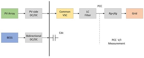
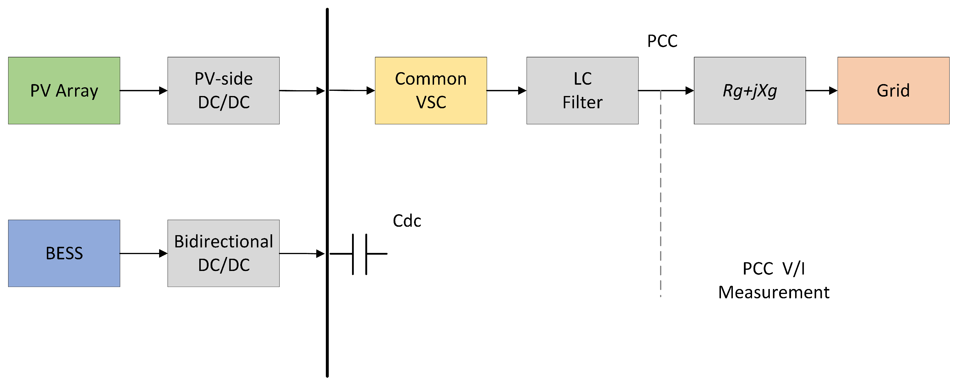
The object of this study is a grid-connected system consisting of a PV array, a BESS, and a VSC, as shown in Figure 1. The DC side includes the PV array, PV-side DC/DC converter, BESS, bidirectional DC/DC converter, and DC-link capacitor. The AC side includes the VSC, LC filter, point of common coupling (PCC), equivalent grid impedance Rg+jXg, and three-phase grid. Renewable-energy grid-connected converters must be coordinately designed with respect to power conversion, grid current quality, and grid support [18]. The BESS can undertake the energy support task in virtual synchronous control through fast power buffering [19].

Figure 1. Structure of the PV-BESS grid-connected system.

The average-value model represents the VSC modulation command as the average AC-side output voltage. It neglects switching ripple while retaining low-frequency dynamics such as power, voltage, and frequency and is therefore suitable for analyzing the effects of grid strength variation and GFL/GFM weight transition on system transients.

2.1.2. DC-Side Power Coordination

Neglecting converter losses, the DC-link power balance is

$$C_{\mathit{dc}}{U}_{\mathit{dc}}{\displaystyle \frac{d{U}_{\mathit{dc}}}{\mathit{dt}}}=P_{\mathrm{PV}}+P_{\mathrm{BESS}}-{\mathrm{P}}_{\mathrm{VSC}}$$

(1)

where P_PV is the PV output power; P_BESS is the BESS charging/discharging power, with P_BESS > 0 indicating discharging; P_VSC is the power absorbed by the VSC from the DC side; C_dc is the DC-link capacitance; and U_dc is the DC-link voltage. The BESS power reference is set as

$$P_{\mathrm{BESS}}^{\ast }=P_g^{\ast }-P_{\mathrm{PV}}+k_{\mathit{dc}}\left(U_{\mathit{dc}}^{\ast }-U_{\mathit{dc}}\right)$$

(2)

where $P_g^{\ast }$ is the grid-connected active power command, $U_{\mathit{dc}}^{\ast }$ is the DC-link voltage reference, and k_dc is the regulation coefficient. In the physical design, the BESS power is saturated according to the upper and lower limits of the state of charge (SOC), so that the main impact of PV fluctuations is confined to the DC side and the response burden on the AC-side controller is reduced. In the reported reduced-order response study, the BESS is represented as an algebraic power buffer: $P_{\mathrm{BESS}}=P_g^{\ast }-P_{\mathrm{PV}}$ is computed at each time step without integrating the battery energy or SOC and without activating an SOC-dependent charging or discharging constraint. The BESS power rating is 300 kW. For Case 4, with $P_g^{\ast }=0.65$ p.u. and the PV output varying between 0.42 and 0.68 p.u., the calculated BESS contribution ranges from +0.23 p.u. (115 kW) to −0.03 p.u. (−15 kW), remaining within the 300 kW rating.

2.1.3. VSC Average-Value Model

Let the three-phase modulation quantity be m_abc and the DC-link voltage be U_dc. The equivalent AC-side output voltage reference is

$$v_{\mathit{inv},\mathit{abc}}^{\ast }={\displaystyle \frac{U_{\mathit{dc}}}{2}}{m}_{\mathit{abc}}$$

(3)

This relationship preserves the dominant link between the modulation quantity and the AC output voltage and can be used to verify the effect of GFL/GFM fusion weight variation on system dynamics.

2.2. Adaptive GFL/GFM Fusion Control

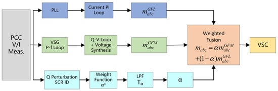
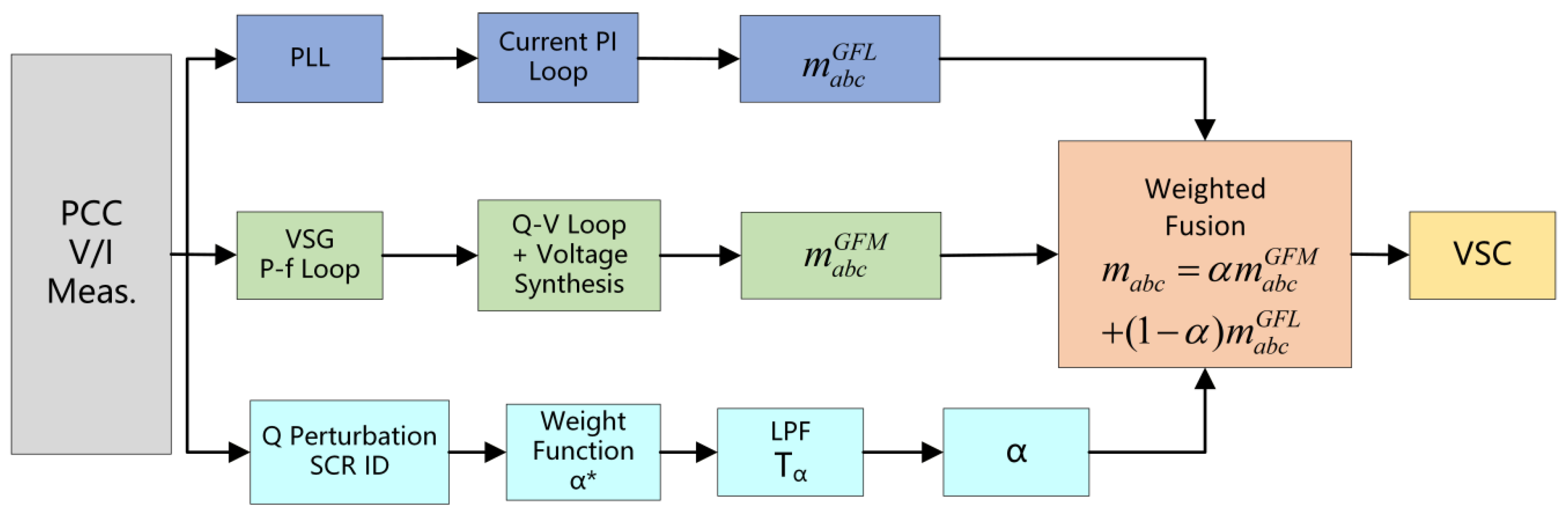
Figure 2 shows the proposed control structure. The GFL and GFM controllers operate in parallel on the same VSC. The online SCR identification module estimates the grid strength in real time, and the continuous weight function and low-pass filter generate the actual fusion weight α. The two modulation waves are fused according to

$$m_{\mathit{abc}}=\alpha m_{\mathit{abc}}^{\mathrm{GFM}}+\left(1-\alpha \right)m_{\mathit{abc}}^{\mathrm{GFL}}, 0\le \alpha \le 1$$

(4)

where $m_{\mathit{abc}}^{\mathrm{GFL}}$ and $m_{\mathit{abc}}^{\mathrm{GFM}}$ are the three-phase modulation waves output by the GFL and GFM channels, respectively. When α = 0, the controller degenerates to pure GFL control; when α = 1, it degenerates to pure GFM control. Because (4) is always a convex combination of the two types of modulation waves, no hard switching of the topology or control structure occurs during the weight variation process, thereby reducing modulation discontinuities at their source.

Figure 2. Structure of the proposed GFL/GFM adaptive fusion control. Here, α∗ denotes the reference GFM fusion weight before low-pass filtering, whereas α denotes the actual GFM fusion weight after low-pass filtering.

The GFL controller adopts the standard structure of a PLL, power outer loop, and current inner loop. With the PCC voltage vector orientation and u_q≈0, the current references corresponding to the power references are

$$i_d^{\ast }={\displaystyle \frac{2P_g^{\ast }}{3u_d}}, i_q^{\ast }=-{\displaystyle \frac{2Q_g^{\ast }}{3u_d}}$$

(5)

where $Q_g^{\ast }$ is the grid-connected reactive power command and u_d is the d-axis component of the PCC voltage. In weak grids, the interaction between the PLL and grid impedance forms a PLL–current loop–grid impedance coupling loop, which may induce power oscillations when the SCR is low.

The GFM controller adopts a virtual synchronous generator (VSG) scheme. The active power–frequency loop is

$$J{\omega }_0{\displaystyle \frac{\mathit{d\omega }}{\mathit{dt}}}=P_g^{\ast }-P_g-D_p(\omega -{\omega }_0)$$

(6)

and the reactive power–voltage loop is

$$E_{\mathit{pu}}^{\ast }=1+n_q\left(Q_{g,\mathit{pu}}^{\ast }-Q_{g,\mathit{pu}}\right)$$

(7)

where U_N = 380 V line-to-line RMS is the voltage base, S_N = 500 kVA is the apparent power base, and n_q = 0.02 p.u./p.u. relates the normalized reactive power deviation to the normalized voltage deviation. The controller is implemented in per-unit quantities for the reactive power–voltage loop, and the rated 380 V line-to-line RMS voltage serves as the base quantity rather than being multiplied directly by the per-unit droop coefficient. Here, J is the virtual inertia, D_p is the active power damping coefficient, ω₀ is the rated angular frequency.

Equation (6) is written in power-balance form; accordingly, D_p has units of W·s/rad, which differs from the torque-form VSG convention, where D_p would carry units of N·m·s/rad and require an additional factor ω₀. The GFM channel achieves autonomous synchronization through negative feedback on the active power deviation without using a PLL; therefore, under weak-grid conditions, it can reduce the risk of synchronization oscillations caused by coupling between the PLL and grid impedance. Virtual synchronous-machine implementations commonly embed virtual inertia, damping, and droop elements into the converter outer loop, so that the converter exhibits approximate synchronous-machine power-angle dynamics under power disturbances. In a PV-BESS system, the BESS provides fast active power buffering and can supply DC-side energy support for the inertia and damping responses of the GFM channel.

From the perspective of control objectives, the GFL channel emphasizes current constraints and fast power tracking, whereas the GFM channel emphasizes voltage angle establishment and weak-grid support. The proposed adaptive fusion control scheme (AFSC) does not simply switch between the two modes. Instead, it uses the SCR estimate to adjust in real time the contribution of each channel to the modulation wave, so that the converter behaves more like a current source in strong grids and more like a voltage source in weak grids. Virtual impedance can improve power sharing and damping in parallel systems by reshaping the converter output impedance. Its compensation for grid strength variation is generally an indirect adjustment at the impedance level and can complement the online update of GFL/GFM weights [20].

A comparison of the proposed AFSC method with representative existing GFL/GFM control approaches is presented in Table 1.

Table 1. Comparison of closely related GFL/GFM methods and the investigated AFSC case across control structures, fusion mechanisms, stability models, coefficient adaptation, and validation.

Method/Source	Control Structure	Fusion Mechanism	Stability Model	Coefficient Adaptation	Validation
Hard switching/state initialization [21,22]	Separate GFL/GFM controllers	Hard switching	Separate pre-/post-switching	Fixed thresholds	Simulation
Virtual impedance/impedance reshaping [23,24]	GFM with virtual impedance	Impedance reshaping	Impedance-based	Indirect	Simulation + measurement
Droop/VSG gain adjustment [25,26]	Droop or VSG	Continuous gain adjustment	Local linearization	Empirical	Simulation
Fixed-structure hybrid control [27,28]	Unified GFL/GFM	Fixed/semi-fixed	Local small-signal	Partial; SCR-based	Inverter case studies
SCR-adaptive hybrid control [29,30]	Adaptive mixed GFL/GFM	Adaptive proportion/hybrid coefficient	Small-signal or impedance-based	SCR-based	Small-signal/impedance analysis and inverter case studies
Proposed method (AFSC)	Parallel GFL/GFM modulation-reference fusion	Bounded piecewise-linear α(SCR) map with first-order filter	Low-order phase margin relation with α	Online SCR identification (0.5 s refresh)	Reduced-order event response study

2.3. Small-Signal Stability Analysis and Parameter Tuning

2.3.1. Small-Signal Model of the Fusion System

Following the classification of power system stability, this paper focuses on converter-dominated small-disturbance synchronization stability under weak-grid conditions [31]. The extended stability definition incorporates converter-driven stability into the power system stability classification framework [32]. On this basis, an engineering small-signal model is constructed by introducing the fusion weight into the dominant weak-grid stability channel. Around the rated operating point, the GFL channel is represented as a synchronization-coupling element formed by the PLL, current loop, and grid impedance, whereas the GFM channel is represented as a voltage-source synchronization element formed by the VSG active power–frequency loop, reactive power–voltage droop, and filter impedance. Because both channels ultimately act on the same modulation wave, the dominant open-loop gain can be approximately expressed as a weighted superposition under a unified base:

G_open,fus(s,α,SCR)≈αG_GFM(s,SCR) + (1 − α)G_GFL(s,SCR)

(8)

Specifically, the SCR variation changes the PCC voltage response and power angle dynamics observed by the VSG loop, thereby influencing the effective synchronization behavior of the GFM channel.

Here, G_GFL(s,SCR) represents the dominant coupling channel formed by the PLL, current loop, and grid impedance, and G_GFM(s,SCR) represents the equivalent synchronization channel of the VSG active power–frequency loop and the reactive power–voltage loop. Grid impedance enters both channels through the shared network and PCC variables. Although the GFM controller does not rely on a PLL for synchronization, its dynamic behavior is still influenced by the SCR through the PCC voltage response, power feedback, and converter–grid interaction. Therefore, both the GFL and GFM channels are implicitly SCR-dependent, and the adaptive coefficient α/alpha adjusts their relative contributions rather than compensating for only the GFL instability. Equation (8) is derived by linearizing the modulation fusion relation

m = (1 − α)m_GFL + αm_GFM

(9)

about a fixed operating point:

δm = (1 − α₀)δm_GFL + α₀δm_GFM + (m_GFM,0 − m_GFL,0)δα

(10)

Equation (8) retains the first two terms for a frozen weight (δα = 0), places both channels on a common base, and neglects cross-coupling and higher-order dynamics. It is an approximate tuning relation, not an exact identity for the complete closed loop.

Equation (8) is a low-order engineering model for scheduling the GFL/GFM fusion weight. To provide an independent small-signal reference, a complete averaged dq-domain AC-side model is established and linearized around the operating point [33]. The state vector is

$$\mathbf{x}={\left[\hspace{0.17em}{i}_{\mathit{fd}},\hspace{0.25em}{i}_{\mathit{fq}},\hspace{0.25em}{v}_{\mathit{cd}},\hspace{0.25em}{v}_{\mathit{cq}},\hspace{0.25em}{i}_{\mathit{gd}},\hspace{0.25em}{i}_{\mathit{gq}},\hspace{0.25em}{\xi }_{\mathit{id}},\hspace{0.25em}{\xi }_{\mathit{iq}},\hspace{0.25em}{\theta }_{\mathrm{PLL}},\hspace{0.25em}{\xi }_{\mathrm{PLL}},\hspace{0.25em}{\delta }_{\mathrm{GFM}},\hspace{0.25em}\Delta {\omega }_{\mathrm{GFM}}\hspace{0.17em}\right]}^T$$

(11)

The grid impedance Zg = Rg + jXg, determined from the SCR value, is included in the dq-axis network equations and modifies the coupling between the converter current and PCC voltage.

The nonlinear model is first linearized around the steady-state operating point (x₀, u₀), and the closed-loop state matrix is obtained as A = ∂f(x, u)/∂x|(x₀, u₀). The grid impedance determined by the SCR value is included in the dq-domain network equations and affects both the GFL and GFM channels through the PCC voltage and current feedback paths. The resulting eigenvalues are used as the reference for evaluating the stability trend of the proposed low-order phase margin model.

With ω₀ = 2πf₀, the electrical subsystem is

$$\begin{array}{cc}\hfill {\displaystyle \frac{d{i}_{\mathit{fd}}}{\mathit{dt}}}& ={\displaystyle \frac{{\omega }_0}{L_{f,\mathit{pu}}}}\left(v_{\mathit{inv},d}-v_{\mathit{cd}}-R_{f,\mathit{pu}}{i}_{\mathit{fd}}\right)+{\omega }_0{i}_{\mathit{fq}},\hfill \\ \hfill {\displaystyle \frac{d{i}_{\mathit{fq}}}{\mathit{dt}}}& ={\displaystyle \frac{{\omega }_0}{L_{f,\mathit{pu}}}}\left(v_{\mathit{inv},q}-v_{\mathit{cq}}-R_{f,\mathit{pu}}{i}_{\mathit{fq}}\right)-{\omega }_0{i}_{\mathit{fd}},\hfill \\ \hfill {\displaystyle \frac{d{v}_{\mathit{cd}}}{\mathit{dt}}}& ={\displaystyle \frac{{\omega }_0}{C_{f,\mathit{pu}}}}\left(i_{\mathit{fd}}-i_{\mathit{gd}}\right)+{\omega }_0{v}_{\mathit{cq}},\hfill \\ \hfill {\displaystyle \frac{d{v}_{\mathit{cq}}}{\mathit{dt}}}& ={\displaystyle \frac{{\omega }_0}{C_{f,\mathit{pu}}}}\left(i_{\mathit{fq}}-i_{\mathit{gq}}\right)-{\omega }_0{v}_{\mathit{cd}},\hfill \\ \hfill {\displaystyle \frac{d{i}_{\mathit{gd}}}{\mathit{dt}}}& ={\displaystyle \frac{{\omega }_0}{X_{g,\mathit{pu}}}}\left(v_{\mathit{cd}}-1-R_{g,\mathit{pu}}{i}_{\mathit{gd}}\right)+{\omega }_0{i}_{\mathit{gq}},\hfill \\ \hfill {\displaystyle \frac{d{i}_{\mathit{gq}}}{\mathit{dt}}}& ={\displaystyle \frac{{\omega }_0}{X_{g,\mathit{pu}}}}\left(v_{\mathit{cq}}-R_{g,\mathit{pu}}{i}_{\mathit{gq}}\right)-{\omega }_0{i}_{\mathit{gd}}.\hfill \end{array}$$

(12)

Grid strength enters through

$$X_{g,\mathit{pu}}={\displaystyle \frac{1}{\mathrm{SCR}}}, R_{g,\mathit{pu}}={\displaystyle \frac{0.1}{\mathrm{SCR}}}$$

(13)

At each pair (SCR,α), the nonlinear equilibrium x₀ is solved numerically, and the complete small-signal model is obtained from the Jacobian

$$\Delta \dot{\mathbf{x}}=\mathbf{A}\left(\mathrm{SCR},\alpha \right)\Delta \mathbf{x}+\mathbf{B}\left(\mathrm{SCR},\alpha \right)\Delta \mathbf{u}$$

(14)

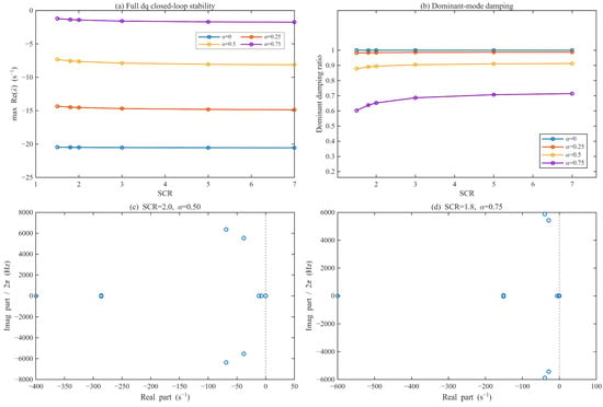
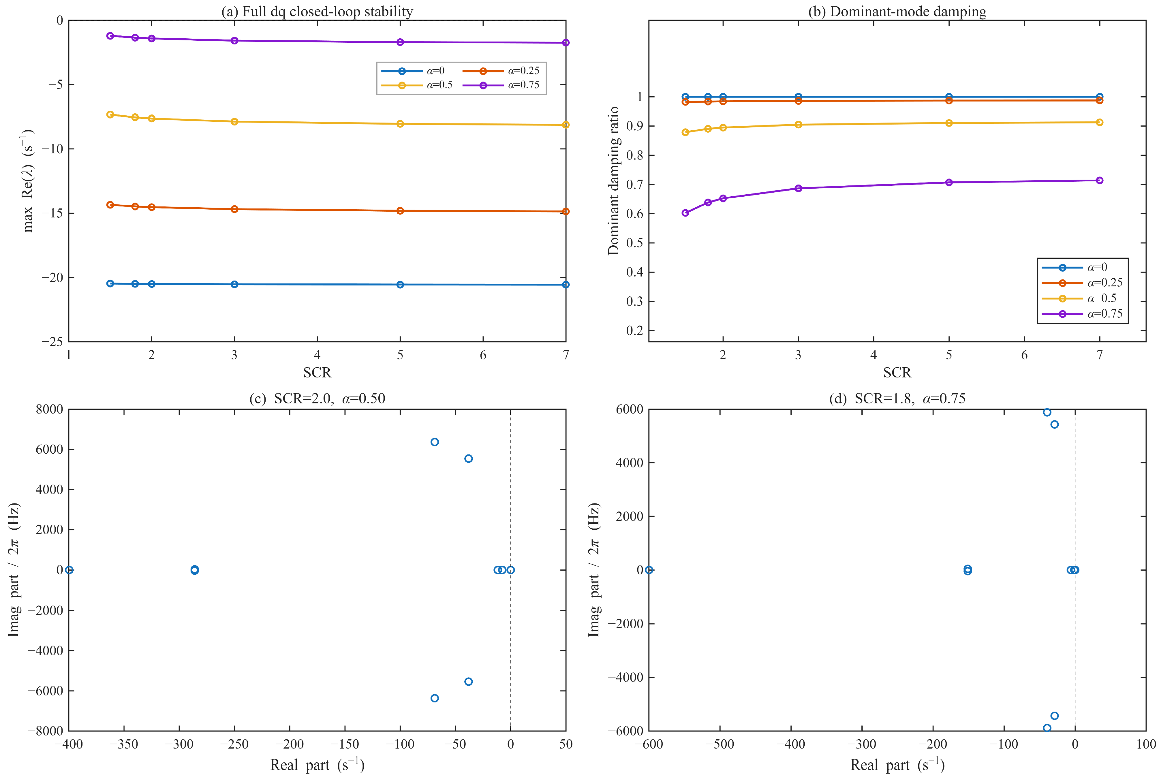
The complete dq model is a multi-input/multi-output closed-loop system. The complete dq-domain validation is therefore carried out through the closed-loop eigenvalues and the dominant synchronization-mode damping over the SCR–α grid. All active modes in the evaluated grid lie in the open left-half plane, and the dominant-mode damping remains positive. At the two representative operating points, the dominant-mode damping ratios are 0.895 (SCR = 2.0, α = 0.50) and 0.638 (SCR = 1.8, α = 0.75), with corresponding dominant-mode frequencies of 0.607 Hz and 0.259 Hz. The complete dq model retains the LC filter dynamics and controller state interactions that are omitted from Equation (8). Figure 3 summarizes the full-dq closed-loop stability, dominant-mode damping, and representative eigenvalue loci used for this validation.

Figure 3. Complete dq-domain small-signal validation: (a) maximum real part of the closed-loop eigenvalues over SCR for selected GFM weights; (b) dominant synchronization-mode damping ratio; (c) eigenvalue locus at SCR = 2.0 and α = 0.50; (d) eigenvalue locus at SCR = 1.8 and α = 0.75. In subfigures (c,d), the blue open circles represent the closed-loop eigenvalues, while the vertical dashed lines indicate Re(λ) = 0, corresponding to the stability boundary between the left and right half-planes.

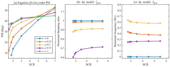
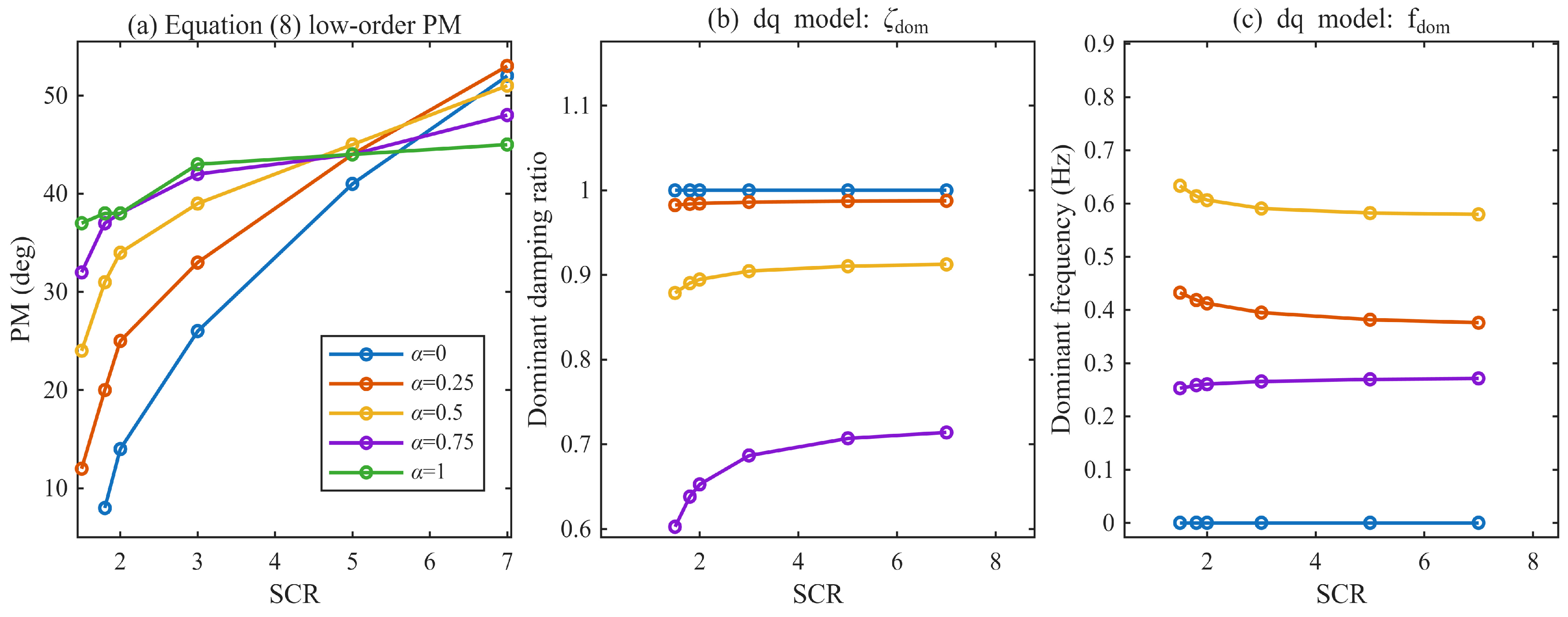
Figure 4 provides a complementary comparison between the low-order phase margin trend and the dominant synchronization-mode characteristics of the complete dq model. The low-order PM increases markedly with GFM participation in weak grids, while the complete dq-domain model retains positive dominant-mode damping across the investigated points.

Figure 4. Low-order and complete dq-domain stability trends versus SCR: (a) Equation (8) low-order phase margin for selected GFM weights; (b) dominant synchronization-mode damping ratio from the complete dq model; (c) corresponding dominant-mode frequency. The colors in subfigures (b,c) correspond to the same GFM weights as indicated by the legend in subfigure (a); the α = 1 case is shown only in subfigure (a).

2.3.2. Effect of GFM Weight on Phase Margin

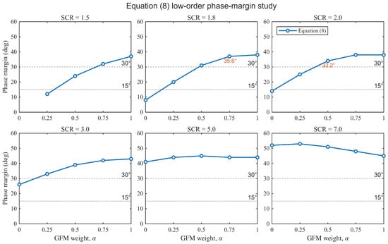
Within the reported low-order parameter study, the phase margin (PM) at crossover is used as an illustrative tuning index, with the values listed in Table 2. A 30° margin is adopted as a case-specific design target, and 15° marks the low-margin portion of the table.

Table 2. System phase margin (°) under different SCRs and GFM weights α.

SCR	α = 0 (100% GFL)	α = 0.25	α = 0.50	α = 0.75	α = 1 (100% GFM)
7.0	52	53	51	48	45
5.0	41	44	45	44	44
3.0	26	33	39	42	43
2.0	14	25	34	38	38
1.8	8	20	31	37	38
1.5	Unstable	12	24	32	37

The 30° value is consistent with widely adopted minimum phase margin guidance in feedback control and power electronics design, where a PM between 30° and 60° is recommended for a satisfactory dynamic response without sustained oscillation [34]. Related stability margin considerations are widely used in grid-connected converter and synchronization-loop design [35,36]. For weak-grid PLL design, the cited study gives a minimum requirement of PM ≥ 30°. The 15° value is consistent with the empirical stability criteria used in converter control practice [37]. In this paper, the 15° value is used only as a design caution marker to identify the low-margin region of the parameter study.

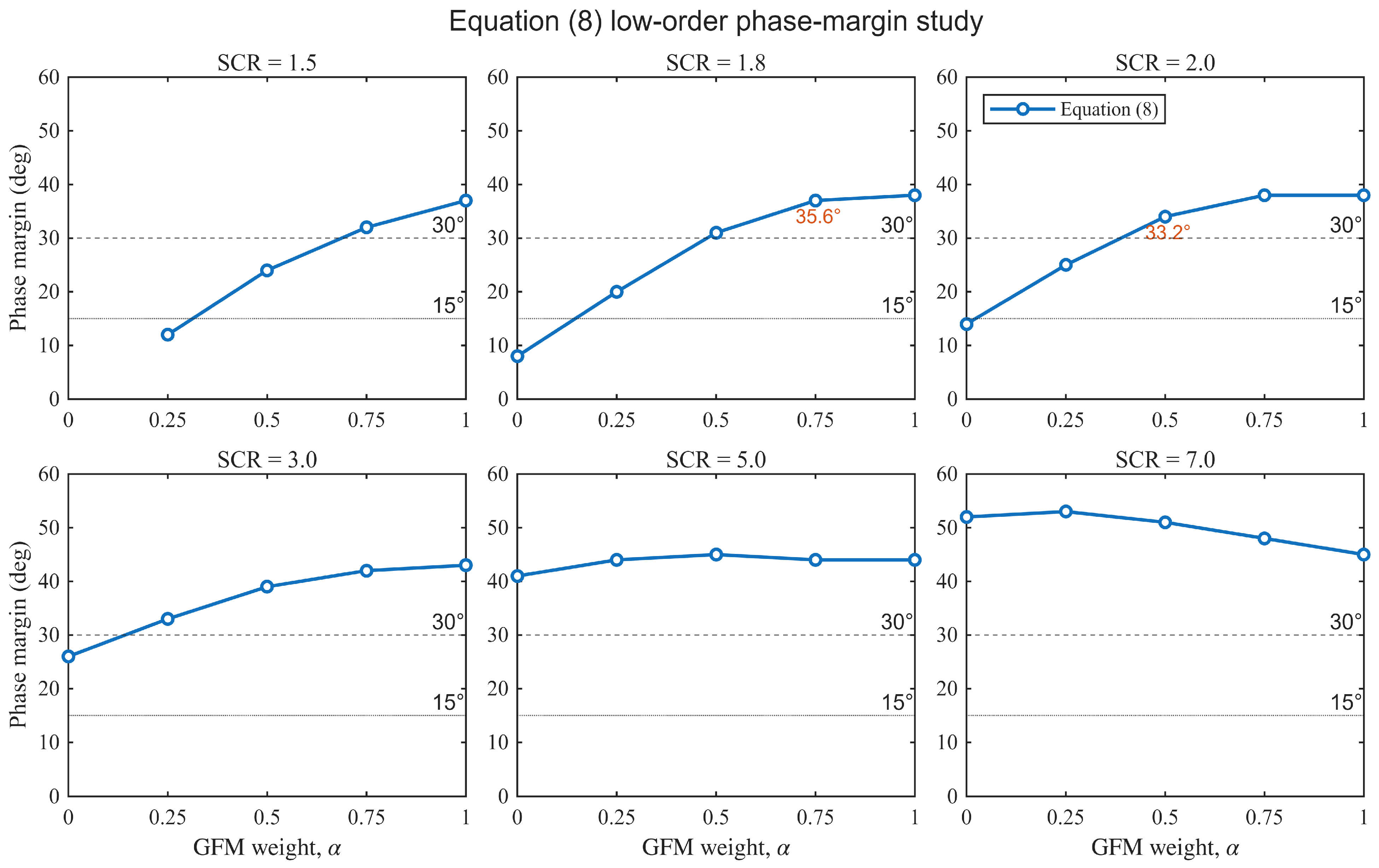
As shown in Table 2, when SCR = 7, the PM of pure GFL control is approximately 52°, satisfying the engineering requirement. However, when the SCR decreases to 1.8, the PM is only 8°, approaching the instability boundary. Under the same condition, increasing α to 0.75 restores the PM to 37°, indicating a significant improvement. Pure GFM control maintains a PM between 38° and 45° under different SCR values and is clearly less sensitive to grid strength variation than pure GFL control. It should be noted that α is not necessarily better when larger: an excessively high GFM weight in a strong grid reduces the power-tracking speed, whereas an excessively low GFM weight in a weak grid cannot provide sufficient voltage-source support. The same low-order phase margin data are plotted in Figure 5 to make the SCR–α dependence and the two representative full-model comparison values directly visible.

Figure 5. Phase margin of the low-order model in Equation (8) under different SCRs and GFM weights.

2.3.3. Tuning Criteria for Key Parameters

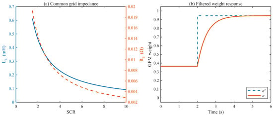
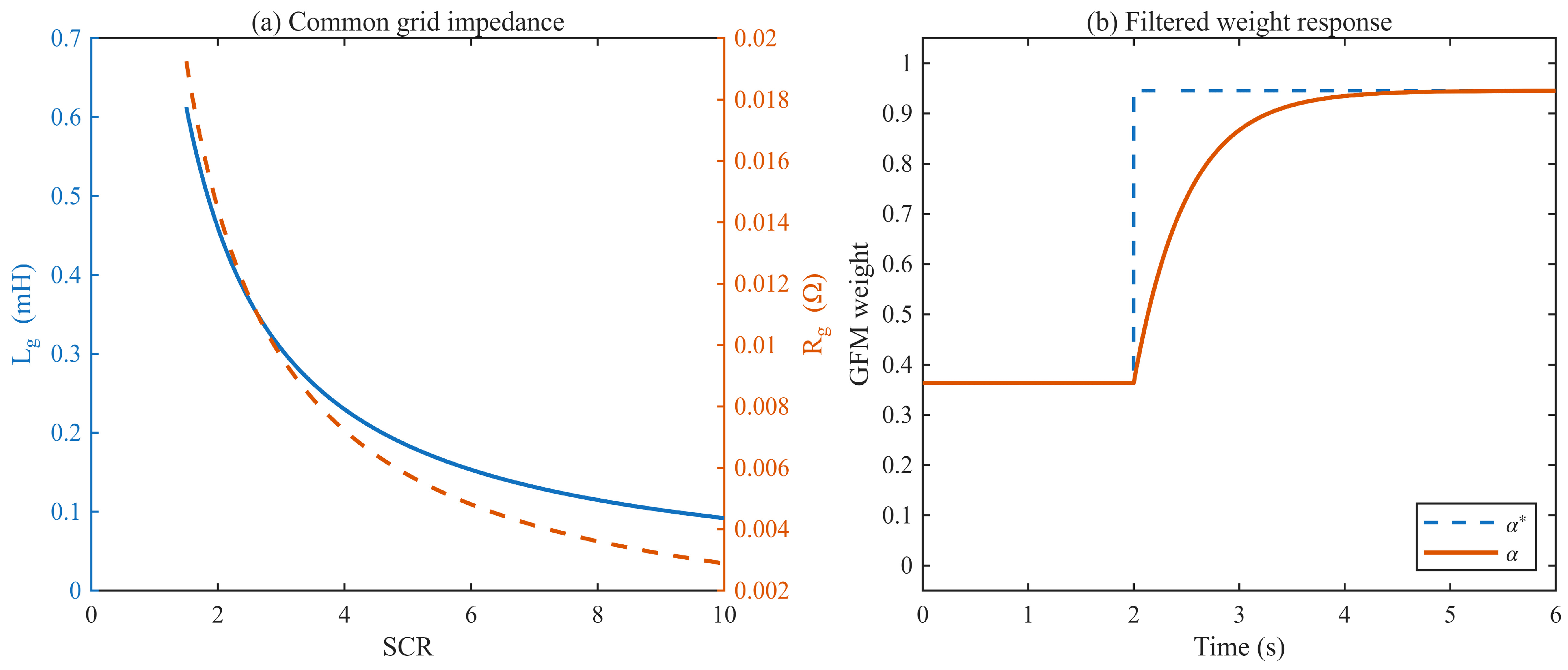
The parameters are tuned by first ensuring weak-grid stability and then preserving the fast response under strong-grid conditions and finally limiting weight dynamics. The extreme weak-grid boundary is set to SCR_low = 1.5. As seen in Table 2, when SCR = 1.5 and α = 1, the PM is approximately 37°, satisfying the weak-stability boundary requirement of PM ≥ 30°. The lower boundary of the strong-grid region in which pure GFL control maintains a relatively high PM is selected as the endpoint of GFM weight attenuation; thus, SCR_high = 7 is adopted. At this point, the PM of pure GFL control is approximately 52°, and the GFM weight can be reduced to 0 to retain fast power-tracking capabilities. The transition interval SCR_high − SCR_low = 5.5 helps to avoid frequent weight chattering under medium grid strength. Finally, the weight-filter time constant T_α should be greater than the dominant variation period of the identification noise but should not be substantially slower than the grid transient process. Considering the SCR identification refresh period T_id = 0.5 s and the typical time scale of grid transients, T_α = 0.5 s is used in this paper. The three key quantities adopted by the algorithm are therefore SCR_low, SCR_high, and T_α. Figure 6a shows the common grid impedance used by both control branches as a function of the SCR, and Figure 6b illustrates the first-order filtered fusion weight response for an SCR change from 5 to 1.8.

Figure 6. SCR-dependent network and weight dynamics used in the AFSC design: (a) common grid inductance Lg and resistance Rg versus SCR; (b) reference GFM weight α* and filtered applied weight α for an SCR step from 5 to 1.8.

2.4. Adaptive Fusion Control Algorithm

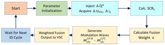
Online SCR identification, the continuous weight function, and low-pass filtering jointly constitute the core of the AFSC algorithm. The SCR identification module provides a real-time estimate of the grid strength, the continuous weight function maps this estimate to the GFM reference weight, and the low-pass filter further limits the rate of weight variation to ensure the continuity of the modulation command.

2.4.1. Online SCR Identification

The proposed physical identification procedure applies a reactive power command perturbation of ΔQ^* = 0.02 p.u. to estimate the equivalent grid impedance and SCR. The perturbation is applied as a rectangular pulse train: a 20 ms rectangular pulse is injected once every identification period T_id = 0.5 s. The pulse waveform is

$$\Delta Q^{\ast }\left(t\right)=\{\begin{array}{ll}0.02 \mathrm{p}.\mathrm{u}.,& 0\le t-k{T}_{\mathit{id}}<20 \mathrm{ms},\\ 0,& \mathrm{otherwise},\end{array}$$

(15)

for each identification period index k = 0,1,2,…. The before/after quantities are obtained from 10 ms averaging windows placed immediately before and after the pulse:

$$\Delta U_{\mathrm{PCC},k}={\overline{U}}_{\mathrm{PCC},k}^{\mathit{after}}-{\overline{U}}_{\mathrm{PCC},k}^{\mathit{before}}, \Delta i_{q,k}={\overline{i}}_{q,k}^{\mathit{after}}-{\overline{i}}_{q,k}^{\mathit{before}}$$

(16)

The 20 ms perturbation duration equals one fundamental period at 50 Hz. The before/after quantities are evaluated using adjacent 10 ms averaging windows. The amplitude ΔQ^* = 0.02 p.u. is a compromise between estimator sensitivity and the deliberate disturbance, corresponding to 2% of the rated reactive power. Measurement filtering and the three-period sliding average described below are used to suppress fundamental frequency and measurement noise components.

$$X_{g,k}={\displaystyle \frac{\Delta U_{\mathrm{PCC},k}}{\Delta i_{q,k}}}, {\mathrm{SCR}}_{\mathit{est},k}={\displaystyle \frac{U_N^2}{S_N{X}_{g,k}}}\approx {\displaystyle \frac{1}{X_{g,k,\mathit{pu}}}}$$

(17)

where k denotes the k-th identification period; U_N is the rated line voltage root mean square value; and S_N is the system rated capacity. The before/after averaging window is T_avg = 10 ms. The sliding-average window applied across identification periods is N_avg = 3, corresponding to a total averaging horizon of 1.5 s. The SCR estimate is saturated to

SCR_est ∈ [SCR_min,SCR_max] = [1.2, 12]

(18)

To first order, the q-axis perturbation estimate in Equation (17) recovers X_g rather than the full impedance magnitude $\left|Z_g\right|=X_g\sqrt{1+{\rho }^2}$. The resulting relative error in the SCR is

$${\displaystyle \frac{{\mathrm{SCR}}_{\mathit{est}}-{\mathrm{SCR}}_{\mathit{true}}}{{\mathrm{SCR}}_{\mathit{true}}}}\approx \sqrt{1+{\rho }^2}-1$$

(19)

where ρ = R_g/X_g. For the investigated grid model with ρ = 0.1, the resulting SCR error is approximately 0.5%; even for ρ = 0.2, the error remains approximately 2.0%.

Measurement filtering is applied before identification. The PCC voltage magnitude and the q-axis current used in the identification are passed through a second-order Butterworth low-pass filter with a cutoff frequency f_m = 500 Hz. This filter removes switching-frequency ripple and high-frequency measurement noise while preserving the fundamental frequency component and the transient associated with the 20 ms perturbation pulse. The filter is applied to both the before and after windows.

Background operating point variations are handled by the differential structure of the identification. Because the before and after windows are adjacent to the perturbation pulse, slow variations in the background operating point (e.g., gradual changes in PV output or grid voltage) affect both windows approximately equally and are largely cancelled out in ΔU_PCC,k and Δi_q,k. Fast variations within a single 30 ms measurement window would introduce errors; to suppress this, the sliding average across N_avg = 3 periods is used. If a large operating point change is detected between consecutive periods, the sliding-average buffer is re-initialized. This re-initialization logic is part of the intended physical implementation; it is not exercised in the reported reduced-order response study because the SCR scheduling signal is prescribed.

2.4.2. Continuous GFM Weight Function

According to the phase margin analysis above, a weaker grid requires a higher GFM weight, whereas a stronger grid should reduce the GFM weight to preserve the fast power-tracking capabilities of GFL control. In Equation (20), SCR denotes the saturated SCR estimate used by the scheduler (i.e., SCR = SCR_est); therefore, the GFM reference weight is defined as

$${\alpha }^{\ast }\left(\mathrm{SCR}\right)=\{\begin{array}{ll}1,& \mathrm{SCR}\le {\mathrm{SCR}}_{\mathit{low}},\\ {\displaystyle \frac{{\mathrm{SCR}}_{\mathit{high}}-\mathrm{SCR}}{{\mathrm{SCR}}_{\mathit{high}}-{\mathrm{SCR}}_{\mathit{low}}}},& {\mathrm{SCR}}_{\mathit{low}}<\mathrm{SCR}<{\mathrm{SCR}}_{\mathit{high}},\\ 0,& \mathrm{SCR}\ge {\mathrm{SCR}}_{\mathit{high}}.\end{array}$$

(20)

Equation (20) is a bounded, with deliberately conservative piecewise-linear interpolation between the two selected SCR endpoints, with slope −1/5.5 in the transition interval. It is not derived as the pointwise minimum-weight solution of phase margin optimization. At SCR = 3, Table 2 gives PM = 33° already at α = 0.25, whereas Equation (20) gives α^* ≈ 0.73. At SCR = 1.8, Table 2 gives PM = 31° already at α = 0.50, whereas Equation (20) gives α^* ≈ 0.95. Equation (20) selects a higher GFM weight as a deliberate design reserve, traded against the active power tracking speed: a larger GFM weight provides an additional damping margin beyond the 30° target under model uncertainty and grid strength estimation errors and reduces the sensitivity of the closed-loop damping to SCR identification noise. The loss in active power tracking speed is bounded, because the GFM weight is reduced to zero as soon as SCR ≥ SCR_high = 7. The phase margin study summarized in Table 2 provides a qualitative trend—a lower SCR requires a higher GFM weight—which motivates the direction of Equation (20).

2.4.3. Weight Low-Pass Filtering

Online SCR estimation inevitably contains sampling noise, response delays to power perturbations, and sliding average errors. If α^* is directly used in (4), the weight will fluctuate with estimation noise and induce high-frequency variations in the modulation wave. Therefore, a first-order low-pass filter is introduced into the weight channel:

$${\displaystyle \frac{\alpha \left(s\right)}{{\alpha }^{\ast }\left(s\right)}}={\displaystyle \frac{1}{T_{\alpha }s+1}}, f_c={\displaystyle \frac{1}{2\pi T_{\alpha }}}$$

(21)

where f_c is the cutoff frequency of the weight channel. When T_α = 0.5 s, f_c is approximately 0.318 Hz, which attenuates high-frequency weight fluctuations near the identification period while not being significantly slower than typical grid transients. In engineering digital control, the following discrete implementation can be adopted:

$${\alpha }_k=\lambda {\alpha }_{k-1}+\left(1-\lambda \right){\alpha }_k^{\ast }, \lambda =\exp \left(-{\displaystyle \frac{T_s}{T_{\alpha }}}\right)$$

(22)

where T_s = 10⁻⁴ s is the controller sampling period and λ = exp(−T_s/T_α) = 0.99980002 is the filter memory factor for T_α = 0.5 s. In the intended physical implementation, the GFL current-loop PI controller, the GFM VSG loops, the PLL, the SCR identification module, and the fusion weight update are all sampled at the same rate T_s = 10⁻⁴ s (10 kHz). This single-rate implementation is adopted for simplicity and to avoid multi-rate coupling effects in the online SCR identification loop. The SCR identification refresh period T_id = 0.5 s is a scheduling-level period, not a sampling-level period; within each refresh period, the SCR estimate is held constant while the fusion weight recursion continues to be updated at T_s = 10⁻⁴ s. The reported reduced-order response study only updates the weight recursion at this time step; the GFL, GFM, PLL, and physical estimator are not separately discretized in this model.

2.4.4. Algorithm Implementation

(1)

Initialize SCR_low, SCR_high, T_α, and the BESS power saturation parameters, and set the initial α to be consistent with the α^* corresponding to the initial SCR estimate.

(2)

During each identification period T_id, inject a small perturbation into the reactive power command, collect ΔU_PCC and Δi_q, calculate the SCR estimate using (17), and apply sliding averaging and saturation.

(3)

Calculate the GFM reference weight α^* according to (20), and update the actual weight α according to (22).

(4)

Run the GFL and GFM controllers separately, obtain the two modulation waves, perform weighted fusion according to (4), and send the fused result to the VSC modulation stage.

In terms of implementation, AFSC changes only the modulation-wave fusion weight and does not alter the hardware topology or the main controller structure. It can therefore be implemented on an existing GFL grid-connected control platform by adding a GFM channel, an online SCR identification module, and a weight-filtering module, which gives the method good engineering portability.

The overall procedure for online SCR identification and adaptive GFL/GFM weight fusion is illustrated in Figure 7.

Figure 7. Flowchart of the online SCR identification and weight fusion algorithm (SCR_k denotes the k-th SCR estimate, SCR_est,k). The asterisk in ΔQ^∗ indicates a reference or commanded quantity. ΔQ^∗ denotes the reactive power reference perturbation (0.02 p.u.) injected for online SCR identification.

3. Results and Discussion

3.1. Simulation Model and Parameters

A reduced-order response study of the defined 500 kVA PV-BESS case was implemented in MATLAB (R2025a, MathWorks, Natick, MA, USA) using the settings in Table 3. Four strategies are compared: pure GFL (α = 0), pure GFM (α = 1), fixed-threshold switching (FTS; α = 1 when SCR_est < 3 and α = 0 otherwise), and AFSC. FTS applies its binary reference directly without the AFSC weight filter. The plotted PCC voltage, power, and current curves follow prescribed event response expressions rather than a solved network-coupled converter model.

Table 3. Simulation parameters of the PV-BESS grid-connected system.

Parameter	Symbol	Value	Unit
System rated capacity	SN	500	kVA
Rated line voltage	UN	380	V
Rated frequency	f0	50	Hz
DC-link voltage reference	$U_{\mathit{dc}}^{\ast }$	800	V
DC-link capacitance	Cdc	10	mF
LC filter inductance	Lf	2	mH
GFL current-loop proportional/integral gain	kp/ki	5/100	—
PLL proportional/integral gain	kp,PLL/ki,PLL	60/1400	—
VSG virtual inertia	J	0.5	kg·m2
VSG active power damping	Dp	10	W·s/rad
Reactive power–voltage droop coefficient	nq	0.02	p.u./p.u.
Lower/upper SCR thresholds	SCRlow/SCRhigh	1.5/7	—
Weight time constant	Tα	0.5	s
Controller sampling period	Ts	1 × 10−4	s
Identification period	Tid	0.5	s
Maximum BESS charging/discharging power	Pmax	300	kW
LC filter capacitance	Cf	2	μF

A 1.5 p.u. fault current design limit is used as the common current ceiling for all four strategies. The limiter is implemented differently for each control structure. For the GFL channel, the current reference is limited by $\left|i_{\mathit{dq}}^{\ast }\right|\le I_{\mathit{max}}=1.5$ p.u., with current-priority allocation [38]:

$$i_d^{\ast }=\min \left(i_{d,0}^{\ast },I_{\mathit{max}}\right), i_q^{\ast }=\mathrm{sign}\left(i_{q,0}^{\ast }\right)\max \left(I_{\mathit{max}}^2-{\left(i_d^{\ast }\right)}^2,0\right)$$

(23)

When the current reference is clipped, the current-controller integrator states are frozen to prevent wind-up. For the GFM channel, a virtual impedance-based voltage limitation is used [39,40]:

$$v_{\mathrm{GFM},\mathit{dq}}^{\ast }=v_{\mathrm{GFM},\mathit{dq}0}-Z_v{i}_{\mathit{dq}}$$

(24)

where Z_v = k_v(|i_dq| − I_th) when |i_dq| ≥ I_th. For FTS, the limiter inherits the current mode. For AFSC, both limiters are applied simultaneously and the two limited modulation waves are fused:

$$v_{\mathit{inv},\mathit{dq}}=\left(1-\alpha \right)v_{\mathrm{GFL},\mathit{dq}}^{\mathit{lim}}+\alpha v_{\mathrm{GFM},\mathit{dq}}^{\mathit{lim}}$$

(25)

In Case 3, the current limiter is not activated because the peak currents remain below 1.5 p.u.

Note: The filter inductance is L_f = 2 mH and the filter capacitance is C_f = 2 μF. The LC resonance frequency is

$$f_{\mathit{LC}}={\displaystyle \frac{1}{2\pi \sqrt{L_f{C}_f}}}\approx 2516 \mathrm{Hz}\approx 2.5 \mathrm{kHz},$$

(26)

which is well above the PLL bandwidth. In the physical design, active damping based on capacitor current feedback is adopted. A virtual resistance R_ad is synthesized by feeding the capacitor current through a gain k_ad into the modulation command:

$$R_{\mathit{ad}}={\displaystyle \frac{1}{k_{\mathit{ad}}}}.$$

(27)

The adopted value is k_ad = 0.2 p.u./p.u., corresponding to R_ad = 5 Ω and a damping ratio of approximately

$${\zeta }_{\mathit{ad}}\approx {\displaystyle \frac{1}{2R_{\mathit{ad}}}}\sqrt{{\displaystyle \frac{L_f}{C_f}}}\approx 0.08.$$

(28)

The grid impedance is converted according to the SCR definition: $X_g=U_N^2/\left(S_N\cdot \mathrm{SCR}\right)$, R_g = 0.1X_g, where U_N is the rated line voltage root mean square value and S_N is the three-phase rated capacity. The corresponding grid inductance is Lg = Xg/ω0.

Statistical definition: The active power recovery time is defined as the time required for the active power to enter and remain within ±2% of the final steady-state value.

3.2. Case 1: Step Change in Grid Strength

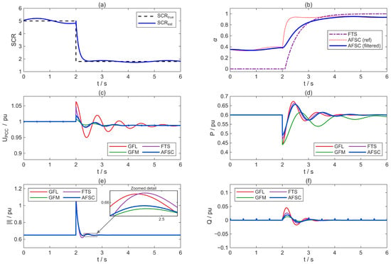
The initial SCR is 5, P_g* = 0.6 p.u., and Qg* = 0. At t = 2 s, tie-line removal is simulated and the SCR decreases to 1.8. This condition is used to examine the changes in SCR identification, fusion weight, voltage oscillation, and current impulse during a transition from a strong grid to a weak grid. The results are shown in Figure 8.

Figure 8. Simulation results under a step decrease in grid strength in Case 1: (a) comparison between the prescribed SCR scheduling input and the true SCR; (b) evolution of the FTS grid-forming mode indicator and the AFSC GFM fusion weight; (c) PCC voltage magnitude; (d) grid-connected active power; (e) converter current magnitude; (f) grid-connected reactive power.

As shown in Figure 8a, after the SCR step change, the prescribed scheduling input reaches the new grid strength level after approximately one refresh period. In Figure 8b, the FTS curve is the grid-forming mode indicator. Because the initial SCR is 5, FTS starts in GFL mode, so β = 0. The AFSC weight α is determined by (20)–(22), and its initial value is approximately 0.36. Therefore, the different starting points of the two curves are not a simulation error. After the SCR decreases, FTS directly crosses the threshold and exhibits a large switching slope, whereas AFSC transitions through the LPF to approximately 0.94 with a smoother variation. Figure 8c–f show that pure GFL control exhibits obvious low-frequency oscillation under the weak-grid condition, with a PCC voltage oscillation amplitude of approximately 0.063 p.u. GFM control has better damping but slower active power recovery. FTS reaches a current peak of 1.15 p.u. at the switching instant. AFSC yields a voltage oscillation amplitude of approximately 0.019 p.u., an active power recovery time of about 2.3 s, and a maximum current of about 1.05 p.u., achieving a favorable tradeoff between stability and power-tracking speed.

3.3. Case 2: Effectiveness of Weight Filtering

This case uses the same SCR step from 5 to 1.8 and compares AFSC with and without the weight LPF. Both runs receive the same synthetic SCR estimation error. The synthetic SCR estimation error is defined as follows. Zero-mean Gaussian noise is added to the SCR estimation input:

$${\mathrm{SCR}}_{\mathit{est}}\left(t_k\right)={\mathrm{SCR}}_{\mathit{true}}\left(t_k\right)+n_k, n_k\sim \mathcal{N}\left(0,{\sigma }_n^2\right).$$

(29)

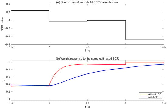
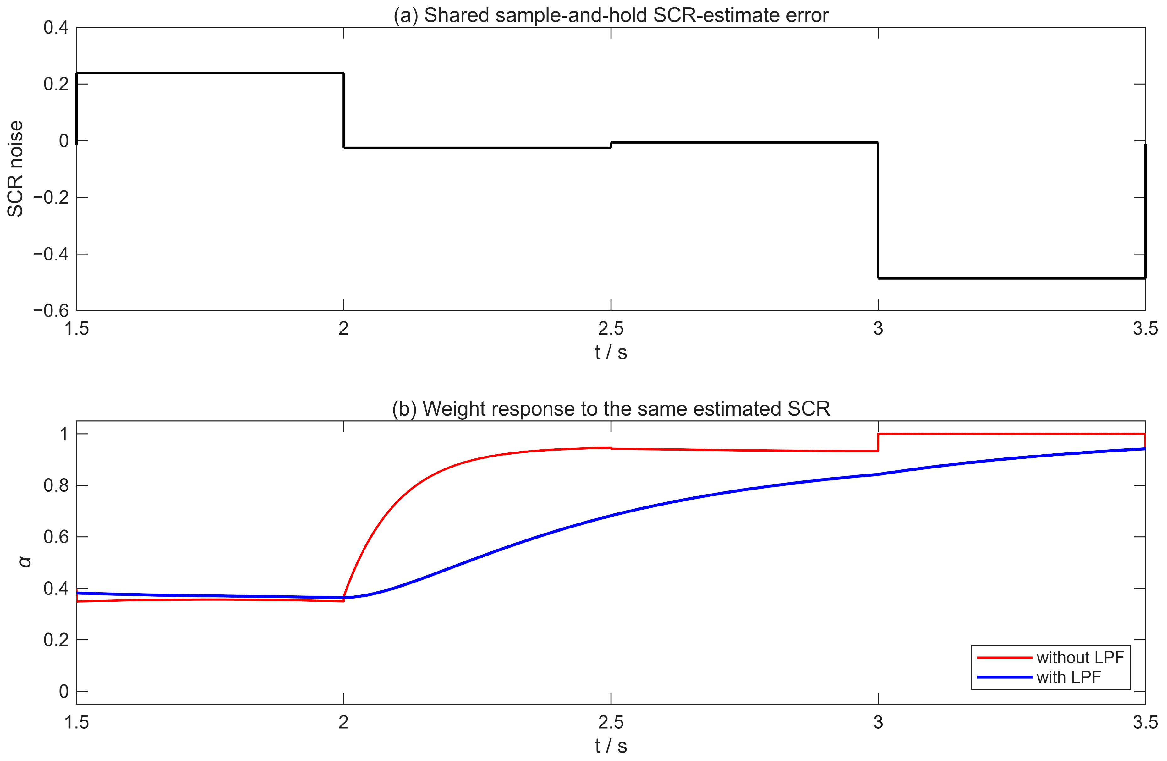
The standard deviation is σ_n = 0.20 SCR units, corresponding to approximately 4% of the SCR value in the range studied. The noise sequence n_k is refreshed once every identification period T_id = 0.5 s and held constant between updates, so the noise entering the weight channel is a zero-order-hold sample-and-hold signal. The random sequence is generated with a fixed random seed (seed 11), so the same noise realization is applied to both the with-LPF and without-LPF runs.

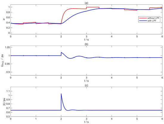
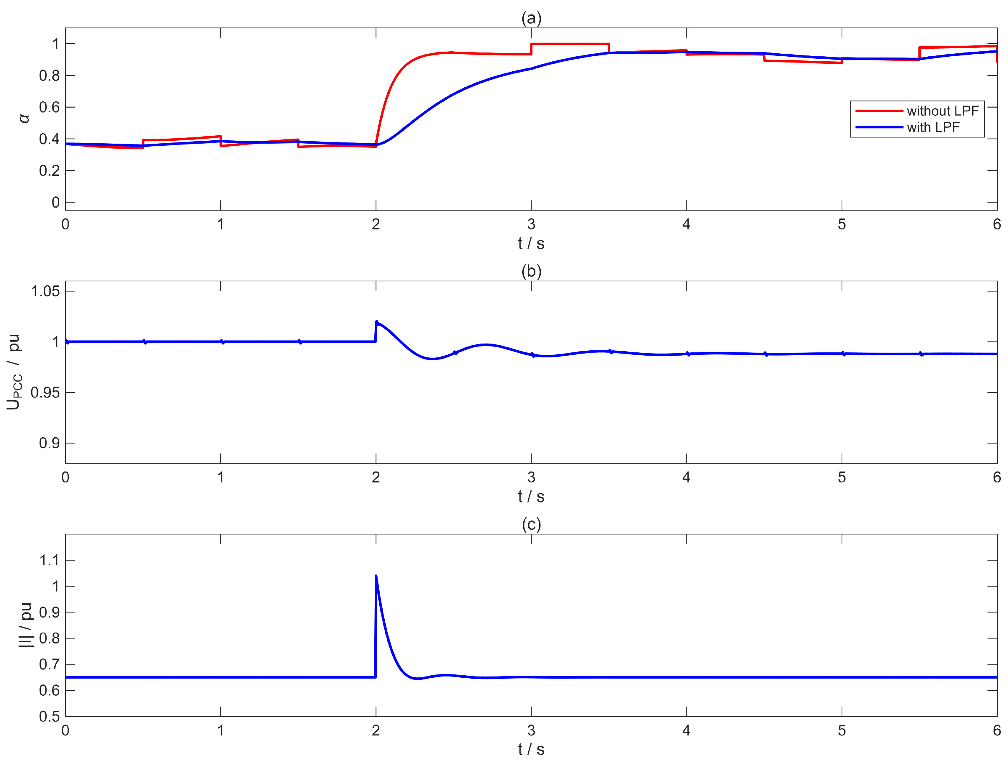
The resulting responses are shown in Figure 9. Figure 9a shows that the unfiltered weight exhibits abrupt changes as the SCR scheduling input changes, whereas the first-order LPF produces a smooth transition toward the new reference value. Figure 9b,c show the corresponding prescribed PCC voltage and converter current response templates. In this reduced-order ablation, these two response templates are the same for the with-LPF and without-LPF cases; therefore, the comparison is used specifically to demonstrate the smoothing of the fusion weight channel rather than to infer an independent change in closed-loop voltage or current stability. With Tα = 0.5 s, the applied weight approaches the reference without overshoot and with a transition rate consistent with the intended bumpless fusion mechanism. Figure 10 shows the shared sample-and-hold SCR estimation error used in both runs and the corresponding fusion weight trajectories with and without the LPF.

Figure 9. Effect of the weight low-pass filter in Case 2: (a) GFM reference weight and applied weight with/without the LPF; (b) prescribed PCC voltage response; (c) prescribed converter current response.

Figure 10. Case 2 SCR estimation error diagnostic: (a) shared sample-and-hold SCR estimation error (standard deviation = 0.20 SCR units, seed 11); (b) resulting GFM fusion weight trajectories with and without the low-pass filter.

3.4. Case 3: Three-Phase Symmetrical Voltage Sag

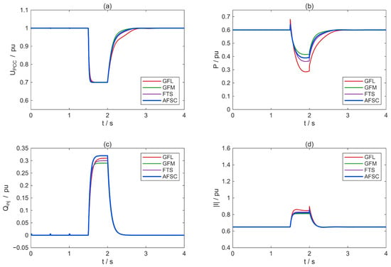
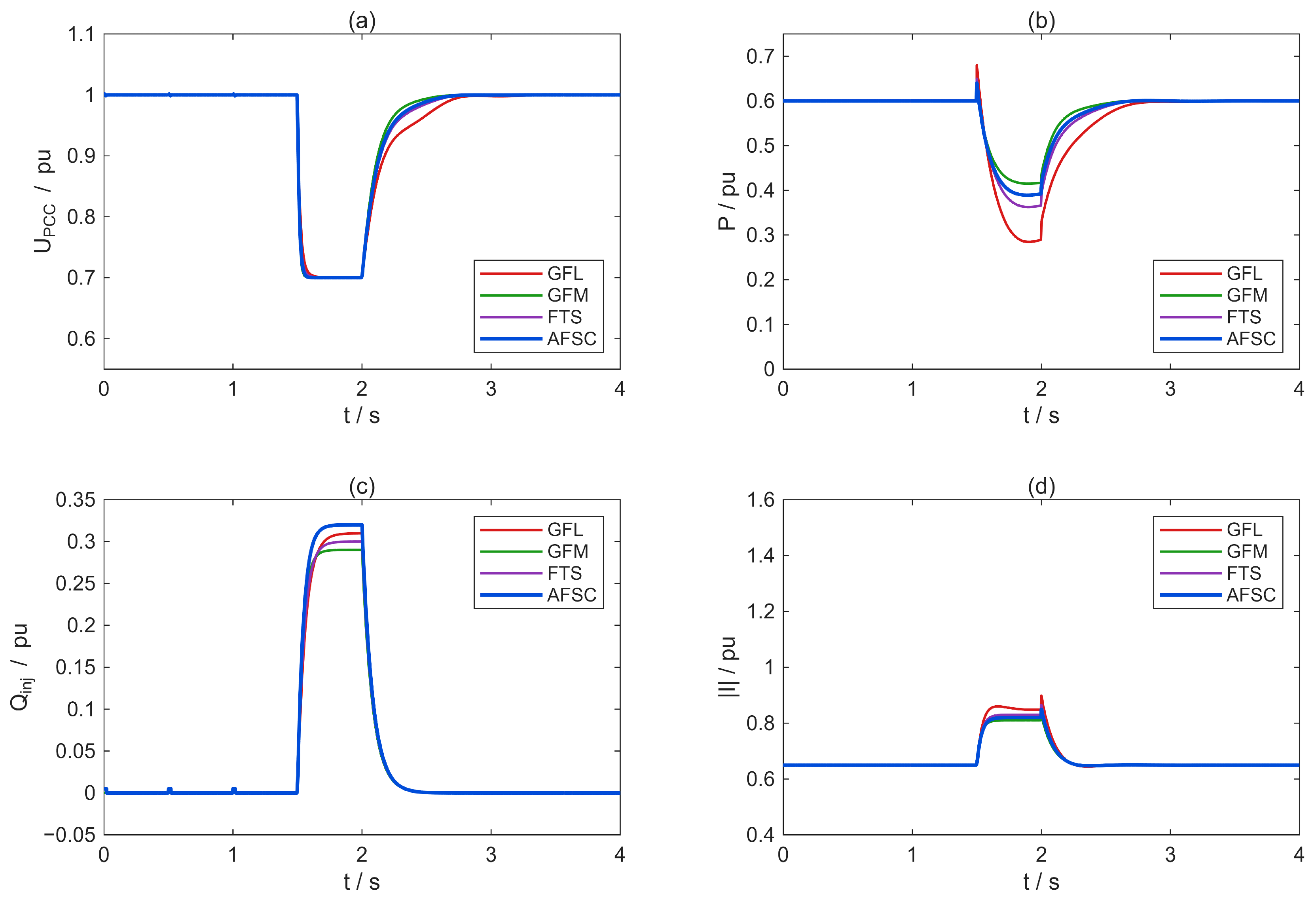
The system operates at SCR = 3. At t = 1.5 s, a three-phase symmetrical voltage sag is applied. In the intended physical network model, the sag is applied at the ideal grid voltage source behind the grid impedance Zg = Rg + jXg. Specifically, the grid-source voltage magnitude is reduced from 1.0 p.u. to 0.7 p.u. for 0.5 s, while the grid impedance and converter-side network remain unchanged. In the reported reduced-order response study, the PCC voltage trajectories are assigned by strategy-dependent event response expressions. This 0.7 p.u./0.5 s profile is an illustrative disturbance rather than a specific grid code requirement. The resulting responses are shown in Figure 11.

Figure 11. Prescribed reduced-order responses under the three-phase symmetrical voltage sag in Case 3: (a) PCC voltage magnitude; (b) grid-connected active power Pg; (c) grid-connected reactive power Qg; (d) converter current magnitude with the 1.5 p.u. design reference.

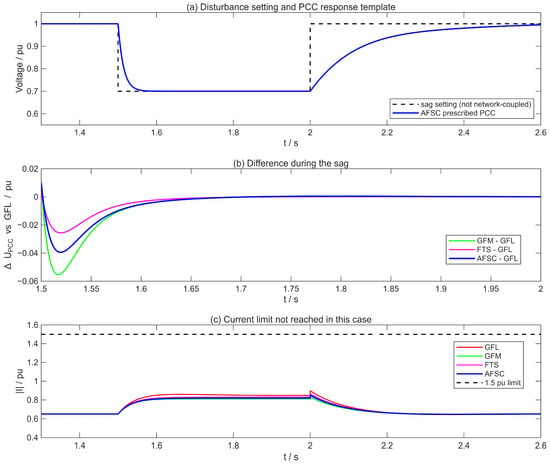
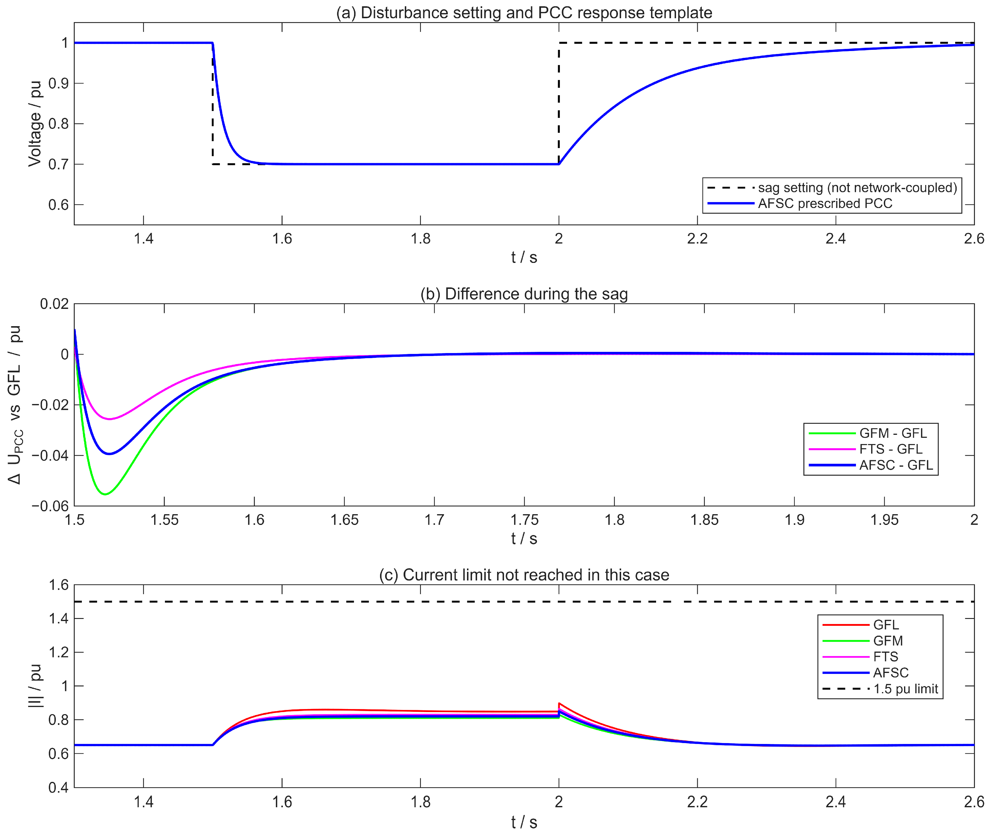
Figure 11 compares the prescribed responses of GFL, GFM, FTS, and AFSC during the voltage sag. The whole-case peak currents are approximately 0.899, 0.830, 0.865, and 0.850 p.u., respectively, all below the 1.5 p.u. design reference shown in Figure 11d. During the 1.5–2.0 s sag, the maximum absolute difference from the GFL PCC voltage curve is approximately 0.055 p.u. for GFM, 0.026 p.u. for FTS, and 0.039 p.u. for AFSC; the corresponding mean absolute deviations are 0.031, 0.017, and 0.024 p.u. The peak reactive power injections are approximately 0.31, 0.29, 0.30, and 0.32 p.u. for GFL, GFM, FTS, and AFSC, respectively. These results provide a direct relative comparison of the four control strategies under the same prescribed voltage sag condition. Figure 12 further isolates the prescribed sag setting, the PCC voltage differences relative to GFL, and the current limit margin for this case.

Figure 12. Case 3 sag diagnostic: (a) prescribed sag setting and PCC voltage response template; (b) PCC voltage difference relative to the GFL curve during the sag; (c) converter current magnitude relative to the 1.5 p.u. design limit.

The maximum voltage differences from the GFL curve during the sag are 0.055 p.u. for GFM, 0.026 p.u. for FTS, and 0.039 p.u. for AFSC.

3.5. Case 4: PV Output Fluctuation

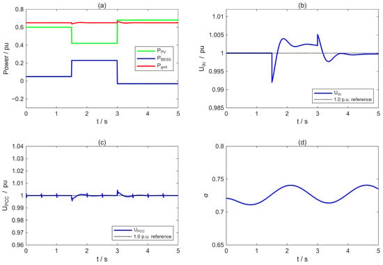
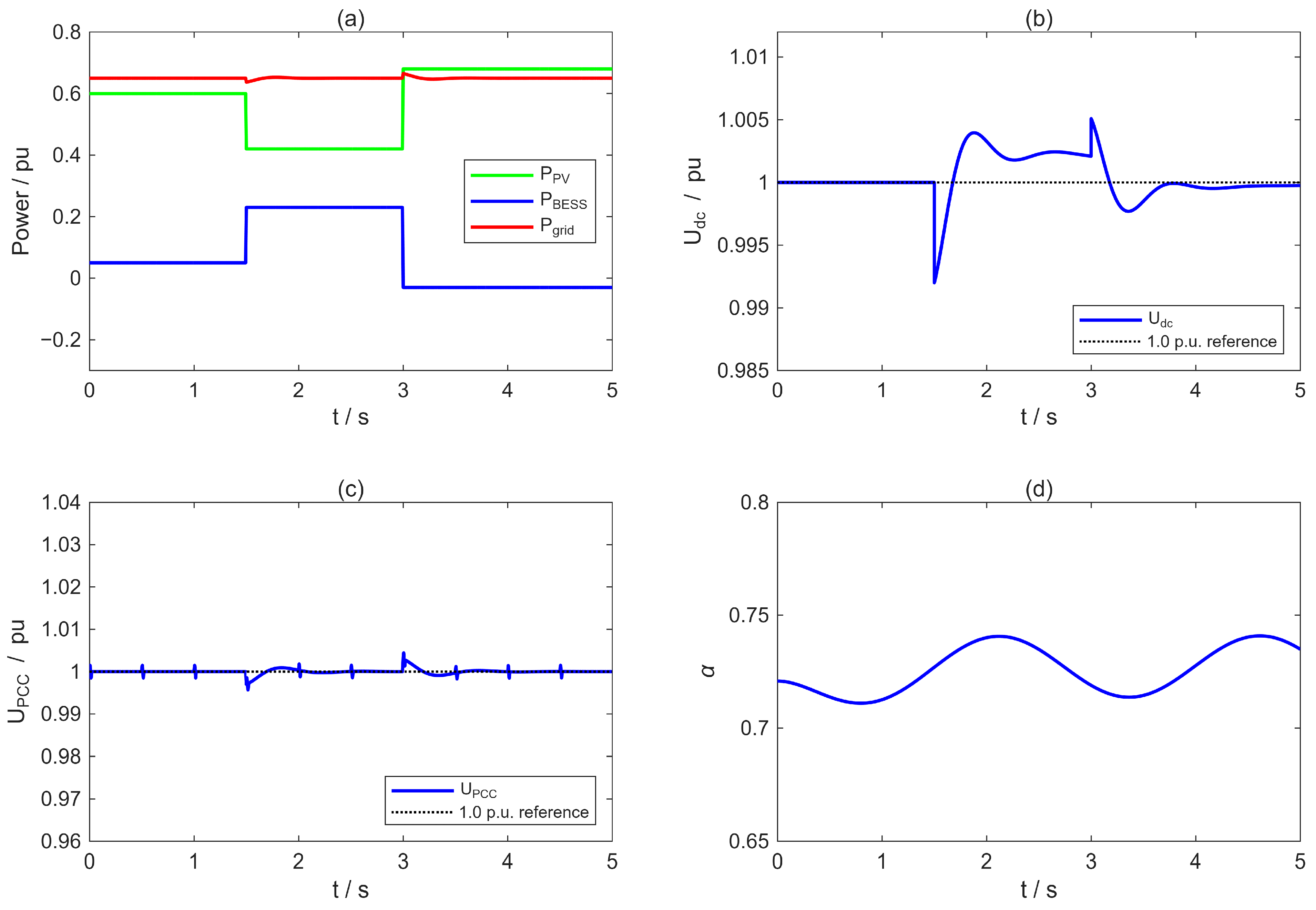
Under SCR = 3 and $P_g^{\ast }=0.65$ p.u., the PV output decreases from 0.60 p.u. to 0.42 p.u. at t = 1.5 s and increases to 0.68 p.u. at t = 3.0 s. This condition mainly examines BESS compensation, DC-link stability, and whether the fusion weight is falsely triggered under source-side power fluctuations. The results are shown in Figure 13.

Figure 13. Simulation results under PV power fluctuations in Case 4: (a) PV, BESS, and grid-connected active power; (b) DC-link voltage; (c) PCC voltage magnitude; (d) GFM fusion weight α. The black dotted lines in subfigures (b,c) indicate the 1.0 p.u. reference values for the DC-link voltage and PCC voltage, respectively.

Figure 13a shows that, when the PV output decreases, the BESS rapidly compensates approximately 0.18 p.u. of power. After the output increases, the BESS absorbs approximately 0.03 p.u. of power, keeping the grid-connected active power close to its command value. In Figure 13b, the maximum DC-link deviation under AFSC is approximately 0.007 p.u. In Figure 13c, the PCC voltage remains stable, and the maximum deviation in the grid-connected active power is approximately 0.015 p.u. Because the grid SCR does not change, the GFM fusion weight in Figure 13d fluctuates only slightly around 0.72, indicating that the weight is governed primarily by the grid strength rather than by the PV-side power disturbance.

3.6. Sensitivity to SCR Input Error

The SCR-to-weight map is evaluated analytically at the nominal true SCR = 3 without assigning a simultaneous Case 1 step disturbance. The operating point is Pg^* = 0.60 p.u. and Qg^* = 0. Prescribed estimate errors of 0%, ±5%, and ±10% are applied to the true SCR = 3.

Reference basis. The reference case is the zero-error case, in which the prescribed SCR estimate equals the true value SCR_est = 3.000. The corresponding reference weight is

$${\alpha }^{\ast }\left(3\right)={\displaystyle \frac{7-3}{7-1.5}}=0.7273.$$

(30)

All signed deviations Δα^* in Table 4 are reported relative to this zero-error reference. By construction, the 0% row has Δα^* = 0.

Table 4. Analytical SCR input error sensitivity and closed-loop stability status of the scheduled GFM weight at true SCR = 3, P^* = 0.60 p.u., Q^* = 0, reference weight α^*(3) = 0.7273.

Estimation Error	Prescribed SCR Estimate	Scheduled α*	Signed Δα*	|Δα*| vs. 0%	Min ζdom	maxRe(λi) s−1)	System Stable
0%	3.000	0.7273	+0.0000	0.0000	0.6938	−1.9505	Yes
+5%	3.150	0.7000	−0.0273	0.0273	0.7203	−2.5021	Yes
−5%	2.850	0.7545	+0.0273	0.0273	0.6762	−1.4754	Yes
+10%	3.300	0.6727	−0.0545	0.0545	0.6729	−3.1215	Yes
−10%	2.700	0.7818	+0.0545	0.0545	0.6828	−1.0878	Yes

Note: The reference basis for all deviations is the zero-error case, in which SCR_est = 3.000 and α^* = 0.7273. Signed Δα^* = α^*(SCR_est) − α^*(3). For each listed input, α^* = (7 − SCR_est)/5.5. These values are calculated directly from the scheduling law in Equation (20). The closed-loop stability status is obtained from the complete dq model of Section 2.3.1. The stability criterion is max_iRe(λ_i) < 0 for the closed-loop eigenvalues and ζ_dom > 0 for the dominant synchronization-mode damping ratio. The operating point is P^* = 0.60 p.u. and Q^* = 0, and no simultaneous grid strength step is applied.

For each of the five error cases, the closed-loop stability is evaluated using the complete dq model of Section 2.3.1. The system is classified as stable if

$$\underset{i}{\max }\mathrm{Re}\left({\lambda }_i\right)<0,$$

(31)

where λ_i are the eigenvalues of the closed-loop Jacobian, and the dominant synchronization-mode damping ratio ζ_dom = −Re(λ_dom)/|λ_dom| is positive.

In all five cases, all active eigenvalues lie in the open left-half plane, and the dominant synchronization-mode damping ratio remains positive.

3.7. Quantitative Comparison

Table 5 lists the quantitative transient performance indices under Case 1, Case 3, and Case 4. Case 2 is not included because it only compares AFSC with and without the weight LPF under identical response templates; it is discussed separately in Section 3.3.

Table 5. Quantitative comparison of transient performance for different control strategies.

Case	Index	Pure GFL	Pure GFM	FTS	AFSC
Case 1	PCC voltage oscillation amplitude/p.u.	0.063	0.008	0.021	0.019
Case 1	Active power recovery time/s	1.8	3.5	2.1	2.3
Case 1	Maximum current impulse/p.u.	1.08	1.02	1.15	1.05
Case 3	Voltage recovery time/s	0.85	0.62	0.70	0.68
Case 3	Peak reactive power injection/p.u.	0.31	0.29	0.30	0.32
Case 4	Maximum DC-link deviation/p.u.	0.010	0.008	0.009	0.007
Case 4	Maximum grid-connected active power deviation/p.u.	0.018	0.025	0.020	0.015

Note: The current impulse of FTS at the switching instant is 1.15 p.u., significantly higher than that of AFSC. The active power recovery time of AFSC lies between those of pure GFL and pure GFM because AFSC retains part of the fast-response characteristic of the GFL channel. Current limiting reshapes the VSG power angle curve and transient stability boundary; therefore, subsequent engineering evaluations should supplement the transient stability margin index under current-limiting modes.

4. Conclusions

This paper has proposed an adaptive GFL/GFM fusion control method based on online SCR identification to address the stability degradation of PV-BESS grid-connected systems under weak-grid conditions. The main conclusions are as follows.

(1)

Small-signal analysis shows that increasing the GFM weight can significantly improve the phase margin under low-SCR conditions. When SCR = 1.8, increasing α from 0 to 0.75 raises the PM from 8° to 37°, providing a quantitative basis for tuning the fusion weight.

(2)

The parameter tuning criteria derived from the phase margin analysis (SCR_low = 1.5, SCR_high = 7 and T_α = 0.5 s) are case-specific settings for the investigated 500 kVA parameterized case. These values reflect the specific stability margins, controller bandwidths, and operating conditions of this case. They are not claimed as universal thresholds or as a transferable parameter set for other PV-BESS systems. A different converter rating, grid impedance, controller bandwidth, or identification scheme requires its own phase margin assessment and parameter selection.

(3)

The continuous weight function and first-order low-pass filter jointly constitute the core of the fusion algorithm, enabling the smooth transition of the modulation wave between GFL and GFM. For the prescribed SCR scheduling trajectory used in the reduced-order study, the 0.5 s refresh period and weight filtering produce the smooth adaptation of the GFM weight; in Case 1, the maximum current impulse is reduced from 1.15 p.u. under FTS to 1.05 p.u. under AFSC.

(4)

The simulation results under four operating conditions demonstrate the effectiveness of the proposed method. Under weak-grid conditions, the PCC voltage oscillation amplitude is approximately 30% of that under pure GFL control, and active power tracking is faster than under pure GFM control. For prescribed SCR input errors of ±10%, the scheduled GFM weight changes by at most 0.055 relative to the zero-error reference, while the complete dq state-space model remains stable for all five evaluated error cases. As high-penetration renewable energy systems evolve toward lower inertia and higher power electronics penetration, future work should further verify the proposed method in multi-converter parallel systems, protection coordination, and grid code-constrained scenarios [41].

References

- Dong, D.; Wen, B.; Boroyevich, D.; Mattavelli, P.; Xue, Y. Analysis of phase-locked loop low-frequency stability in three-phase grid-connected power converters considering impedance interactions. IEEE Trans. Ind. Electron. 2015, 62, 310–321. [Google Scholar] [CrossRef] [Scilit]
- Zhang, L.; Harnefors, L.; Nee, H.P. Power-synchronization control of grid-connected voltage-source converters. IEEE Trans. Power Syst. 2010, 25, 809–820. [Google Scholar] [CrossRef] [Scilit]
- Lasseter, R.H.; Chen, Z.; Pattabiraman, D. Grid-forming inverters: A critical asset for the power grid. IEEE J. Emerg. Sel. Top. Power Electron. 2020, 8, 925–935. [Google Scholar] [CrossRef] [Scilit]
- Rocabert, J.; Luna, A.; Blaabjerg, F.; Rodriguez, P. Control of power converters in AC microgrids. IEEE Trans. Power Electron. 2012, 27, 4734–4749. [Google Scholar] [CrossRef] [Scilit]
- Rathnayake, D.B.; Akrami, M.; Phurailatpam, C.; Me, S.P.; Hadavi, S.; Jayasinghe, G.; Zabihi, S.; Bahrani, B. Grid forming inverter modeling, control, and applications. IEEE Access 2021, 9, 114781–114807. [Google Scholar] [CrossRef] [Scilit]
- Zhang, H.; Xiang, W.; Lin, W.; Wen, J. Grid forming converters in renewable energy sources dominated power grid: Control strategy, stability, application, and challenges. J. Mod. Power Syst. Clean Energy 2021, 9, 1239–1256. [Google Scholar] [CrossRef] [Scilit]
- Geng, S.; Hiskens, I.A. Unified grid-forming/following inverter control. IEEE Open Access J. Power Energy 2022, 9, 489–500. [Google Scholar] [CrossRef] [Scilit]
- Zhong, Q.C.; Weiss, G. Synchronverters: Inverters that mimic synchronous generators. IEEE Trans. Ind. Electron. 2011, 58, 1259–1267. [Google Scholar] [CrossRef] [Scilit]
- Sun, J. Impedance-based stability criterion for grid-connected inverters. IEEE Trans. Power Electron. 2011, 26, 3075–3078. [Google Scholar] [CrossRef] [Scilit]
- Cespedes, M.; Sun, J. Impedance modeling and analysis of grid-connected voltage-source converters. IEEE Trans. Power Electron. 2014, 29, 1254–1261. [Google Scholar] [CrossRef] [Scilit]
- Wen, B.; Boroyevich, D.; Burgos, R.; Mattavelli, P.; Shen, Z. Analysis of dq small-signal impedance of grid-tied inverters. IEEE Trans. Power Electron. 2016, 31, 675–687. [Google Scholar] [CrossRef] [Scilit]
- Han, F.; Zhang, X.; Li, M.; Li, F.; Zhao, W. Stability control for grid-connected inverters based on hybrid-mode of grid-following and grid-forming. IEEE Trans. Ind. Electron. 2024, 71, 10750–10760. [Google Scholar] [CrossRef] [Scilit]
- Liu, P.; Xie, X.; Shair, J. Adaptive hybrid grid-forming and grid-following control of IBRs with enhanced small-signal stability under varying SCRs. IEEE Trans. Power Electron. 2024, 39, 6603–6607. [Google Scholar] [CrossRef] [Scilit]
- Liu, P.; Xie, X.; Miao, Q.; Su, K.; Huo, Y.; Wang, X. Adaptive grid-forming and grid-following hybrid control and its mechanism for enhancing converter’s oscillatory stability. Proc. CSEE 2025, 45, 6062–6069. [Google Scholar] [CrossRef]
- Chao, W.; Dai, L.; Feng, Y.; Huang, J.; Wang, J.; Lin, X.; Zhang, C. Adaptive hybrid grid-following and grid-forming control with hybrid coefficient transition regulation for transient current suppression. Energies 2026, 19, 549. [Google Scholar] [CrossRef] [Scilit]
- Liao, Z.; Hu, Q.; Huang, Z.; Ge, J.; Yang, D.; Ma, X. A seamless transition control strategy based on adaptive fusion between grid-following and grid-forming inverters for wide-ranging grid-strength fluctuations. Electronics 2026, 15, 1298. [Google Scholar] [CrossRef] [Scilit]
- Henderson, C.; Egea-Alvarez, A.; Knueppel, T.; Yang, G.; Xu, L. Grid strength impedance metric: An alternative to SCR for evaluating system strength in converter-dominated systems. IEEE Trans. Power Deliv. 2024, 39, 386–396. [Google Scholar] [CrossRef] [Scilit]
- Carrasco, J.M.; Franquelo, L.G.; Bialasiewicz, J.T.; Galvan, E.; Portillo, R.C.; Prats, M.A.M.; Leon, J.I.; Moreno-Alfonso, N. Power-electronic systems for the grid integration of renewable energy sources: A survey. IEEE Trans. Ind. Electron. 2006, 53, 1002–1016. [Google Scholar] [CrossRef] [Scilit]
- Fang, J.; Tang, Y.; Li, H.; Li, X. A battery/ultracapacitor hybrid energy storage system for implementing the power management of virtual synchronous generators. IEEE Trans. Power Electron. 2018, 33, 2820–2824. [Google Scholar] [CrossRef] [Scilit]
- He, J.; Li, Y.W. Analysis, design, and implementation of virtual impedance for power electronics interfaced distributed generation. IEEE Trans. Ind. Appl. 2011, 47, 2525–2538. [Google Scholar] [CrossRef] [Scilit]
- Ruan, H.; Xiao, Y.; Yang, Y.; Luo, H.; Blaabjerg, F. A plug-and-play switching strategy for seamless transition between grid-following and grid-forming control modes. IEEE Trans. Ind. Appl. 2026. [Google Scholar] [CrossRef] [Scilit]
- Zhang, Z.; Yan, J.; Shi, X.; Wang, Z.; Lin, L. A switching method for seamless transitions between grid-following and grid-forming control without inner current loop. In Proceedings of the IECON 2025—51st Annual Conference of the IEEE Industrial Electronics Society, Madrid, Spain, 14–17 October 2025. [Google Scholar] [CrossRef] [Scilit]
- Wu, L.; Bao, Y.; Xian, L.; Qiu, N.; Chen, W. Reactive power coordination control strategy of multi-parallel network converter. Glob. Energy Interconnect. 2025, 8, 918–930. [Google Scholar] [CrossRef] [Scilit]
- Lou, M.; Meng, J.; Liu, H.; Yu, S. Coordinated control strategy of multi-time-scale virtual impedance for grid-forming converters under weak grid conditions. In Proceedings of the 2026 7th International Conference on Electrical Technology and Automatic Control (ICETAC), Nanjing, China, 12–14 June 2026; pp. 182–186. [Google Scholar] [CrossRef] [Scilit]
- Liu, H.; Wang, H.; Huang, H.; Zhang, M.; Zhang, X. Stability analysis and parameter optimization method of multiple grid-forming converter system with VSG and droop control. Glob. Energy Interconnect. 2026, 9, 828–841. [Google Scholar] [CrossRef] [Scilit]
- Zhou, X.; Zhang, L.; Peng, H.; Hong, L.; Xu, Q.; Zhang, Z.; Shao, J.; Ma, J.; Hu, Y. An improved grid-forming control method with adaptive virtual impedance combining current limitation and transient stability improvement. Int. J. Electr. Power Energy Syst. 2026, 175, 111659. [Google Scholar] [CrossRef] [Scilit]
- Nag, S.; Qu, Z.; Xu, Y. A unified grid-forming and grid-following primary control design with optimized enforcement of grid operational constraints. IEEE Access 2023, 11, 57415–57427. [Google Scholar] [CrossRef] [Scilit]
- Ingalalli, A.; Aygun, A.I.; Kamalasadan, S. A unified control design of three phase inverters suitable for both grid-forming and following modes of operation. IET Renew. Power Gener. 2025, 19, e70043. [Google Scholar] [CrossRef] [Scilit]
- Pavankumar, Y.; Luo, X.; Batzelis, S.I.; Singh, A.K.; Saridaki, G.; Kotsampopoulos, P.; Hatziargyriou, N. Seamless transition between grid forming and grid following inverters based on online grid impedance estimation. In Proceedings of the 2025 IEEE Power & Energy Society General Meeting (PESGM), Austin, TX, USA, 27–31 July 2025; pp. 1–5. [Google Scholar] [CrossRef] [Scilit]
- Zheng, X.; Yang, S.; Xie, Z.; Zhang, X. Equivalence of grid-tied inverters operating in the grid-following and grid-forming modes just through adapting the control parameters. IEEE Trans. Energy Convers. 2026, 1–14. [Google Scholar] [CrossRef] [Scilit]
- Kundur, P.; Paserba, J.; Ajjarapu, V.; Andersson, G.; Bose, A.; Canizares, C.; Hatziargyriou, N.; Hill, D.; Stankovic, A.; Taylor, C.; et al. Definition and classification of power system stability IEEE/CIGRE joint task force on stability terms and definitions. IEEE Trans. Power Syst. 2004, 19, 1387–1401. [Google Scholar] [CrossRef] [Scilit]
- Hatziargyriou, N.; Milanovic, J.V.; Rahmann, C.; Ajjarapu, V.; Canizares, C.; Erlich, I.; Hill, D.J.; Hiskens, I.A.; Kamwa, I.; Pal, B.; et al. Definition and classification of power system stability—Revisited and extended. IEEE Trans. Power Syst. 2021, 36, 3271–3281. [Google Scholar] [CrossRef] [Scilit]
- Harnefors, L. Modeling of three-phase dynamic systems using complex transfer functions and transfer matrices. IEEE Trans. Ind. Electron. 2007, 54, 2239–2248. [Google Scholar] [CrossRef] [Scilit]
- Erickson, R.W.; Maksimovic, D. Fundamentals of Power Electronics, 3rd ed.; Springer: Cham, Switzerland, 2020. [Google Scholar] [CrossRef] [Scilit]
- Franklin, G.F.; Powell, J.D.; Emami-Naeini, A. Feedback Control of Dynamic Systems, 8th ed.; Pearson: Harlow, UK, 2019. [Google Scholar]
- Li, G.; Pan, H.; Liu, X.; Yin, L.; Goh, H.H. PLL phase margin design and analysis for mitigating sub/super-synchronous oscillation of grid-connected inverter under weak grid. Int. J. Electr. Power Energy Syst. 2023, 151, 109124. [Google Scholar] [CrossRef] [Scilit]
- Blaabjerg, F.; Teodorescu, R.; Liserre, M.; Timbus, A.V. Overview of control and grid synchronization for distributed power generation systems. IEEE Trans. Ind. Electron. 2006, 53, 1398–1409. [Google Scholar] [CrossRef] [Scilit]
- Taul, M.G.; Wang, X.; Davari, P.; Blaabjerg, F. Current limiting control with enhanced dynamics of grid-forming converters during fault conditions. IEEE J. Emerg. Sel. Top. Power Electron. 2020, 8, 1062–1073. [Google Scholar] [CrossRef] [Scilit]
- Chen, J.; Prystupczuk, F.; O’Donnell, T. Use of voltage limits for current limitation in grid-forming converters. CSEE J. Power Energy Syst. 2020, 6, 259–269. [Google Scholar] [CrossRef] [Scilit]
- Ordono, A.; Sanchez-Ruiz, A.; Zubiaga, M.; Asensio, F.J.; Cortajarena, J.A. Current limiting strategies for grid forming inverters under low voltage ride through. Renew. Sustain. Energy Rev. 2024, 202, 114657. [Google Scholar] [CrossRef] [Scilit]
- Kroposki, B.; Johnson, B.; Zhang, Y.; Gevorgian, V.; Denholm, P.; Hodge, B.M.; Hannegan, B. Achieving a 100% renewable grid: Operating electric power systems with extremely high levels of variable renewable energy. IEEE Power Energy Mag. 2017, 15, 61–73. [Google Scholar] [CrossRef] [Scilit]
Disclaimer/Publisher’s Note: The statements, opinions and data contained in all publications are solely those of the individual author(s) and contributor(s) and not of MDPI and/or the editor(s). MDPI and/or the editor(s) disclaim responsibility for any injury to people or property resulting from any ideas, methods, instructions or products referred to in the content. |
© 2026 by the authors. Licensee MDPI, Basel, Switzerland. This article is an open access article distributed under the terms and conditions of the Creative Commons Attribution (CC BY) license.