


Abstract
This review examines when neural networks can replace or accelerate finite-rate chemistry in combustion simulations. It analyzes how reaction-step errors propagate, computes the accuracy each target requires for methane, hydrogen, and ammonia/hydrogen, and assesses 125 studies against these requirements. Set by the true increment of the state per step, they differ between targets. The ignition delay responds logarithmically to a bias but nearly proportionally to a relative error in the radical increments where the radicals carry the explosive mode, as in hydrogen below the extended second explosion limit. For NO, the formation route matters: thermal NO responds linearly to a bias accumulated over the residence time, whereas fuel NO forms with large increments during ignition. Root-mean-square errors reported for a hydrogen flame exceed the computed bias tolerances of hydrogen ignition by three to six orders of magnitude and cannot show whether ignition is predicted. In controlled comparisons, coverage of the flow states, exact element conservation, and training on sequences of steps made coupled runs stable. Networks reproduced flame speeds and mean temperatures within a few percent; low-temperature ignition, extinction, nitrogen species, and heat loss needed training aimed at their states and time scales. With equal hardware and mechanisms, networks accelerated the chemistry about tenfold and whole simulations a few times, within the bound set by the chemistry share.
1. Introduction
Gas turbines, engines, and furnaces are being adapted to hydrogen, ammonia, and their blends with hydrocarbons, and the processes that decide whether these fuels can be burned cleanly and stably (ignition, flame stabilization, extinction, and the formation of NO and N2O) are controlled by finite-rate chemistry [1]. Predicting them requires reaction mechanisms with tens to thousands of species, and integrating their stiff kinetic equations in every cell and time step often dominates the cost of a reacting-flow simulation. In LES-PDF of a piloted methane jet flame with a 38-species mechanism, 65% of the run time was spent in the reaction step [2], and the share grows with the size of the mechanism [3]. Mechanism reduction, tabulation [4], implicit solvers with analytical Jacobians [5,6], and GPU integrators [7,8] have lowered this cost, and since the mid-1990s, neural networks have been trained to stand in for the reaction step itself [9,10,11].
Deep networks of several kinds are now applied to the problem, solver frameworks make them usable in production codes [12,13], and network chemistry has been run on tens of thousands of supercomputer nodes [14]. The reported speedups range from a slowdown to about , and the evidence behind them extends from single-step errors on held-out states to LES of practical combustors. These reports do not yet answer the question a combustion modeler faces: for which quantities, flames, and conditions can a network replace the chemistry of a CFD solver, and how much shorter does the simulation then become? Accuracy is mostly reported as an error per step averaged over the test states, which does not show how errors grow when the network is applied to its own output in a flow; and speedups mix the gain of the method with those of the hardware, the reference solver, and the mechanism.
Previous reviews of machine learning in combustion include network chemistry among other topics [15,16,17], and two recent preprints propose reporting standards for chemistry surrogates and manifold models [18,19]. Their coverage is compared in Table S9 of the Supplementary Materials. This review combines an analysis of the reaction step with an assessment of the evidence. It derives the accuracy each combustion target requires from the modes of the reaction step, the states that transport creates, and the propagation of errors over repeated calls; it quantifies these requirements with calculations of the exact reaction map for methane, hydrogen, and ammonia/hydrogen; and it uses them to assess the evidence on combustion predictions and cost, quantity by quantity. The evidence comprises 125 studies published between 1995 and 2026, found by a documented search (Appendix A), read in full, and coded on the same criteria.
Three findings result. First, the accuracy a combustion target requires is set by the true increments of the reaction step, that is, by how much the state changes over one time step, and errors averaged over all test states cannot show whether a network meets it. For ignition, the ignition regime decides which species a network must reproduce in relative terms, and the computational singular perturbation (CSP) pointer of the explosive mode identifies these species; for NO, the required accuracy depends on whether NO forms in the flame front or in the post-flame gas.
Second, in controlled comparisons, coverage of the flow states, exact element conservation, and training on sequences of steps made coupled runs stable. Networks reproduced flame speeds and mean temperatures within a few percent, whereas low-temperature ignition, extinction, nitrogen species, and heat loss were reproduced only with training aimed at their states and time scales. Extinction limits and flame–wall quenching have not yet been predicted. Third, the gain is bounded by the share of the run time spent in the chemistry: on equal hardware and with the same mechanism, networks have made the chemistry about ten times and the simulation a few times faster, for mechanisms of a few tens of species.
The scope is finite-rate chemistry: regression of flamelet and manifold tables and subgrid reaction-rate closures are discussed only where they bear on the argument. Section 2 derives the physical requirements, the following sections review how networks meet them in coupled simulations and at what cost, and Section 8 states when a network can replace the reaction step and which problems, including plasma-assisted combustion, remain open.
2. The Reaction Step in a Flow Solver: Time Scales, Composition Space, and Error Propagation
A network for finite-rate chemistry replaces or assists one operation of a reacting-flow solver: integrating the chemical source terms over a time step, called the reaction step in what follows. What this operation must preserve, and where an approximation is fragile, follows from the structure of chemical kinetics and from how transport couples the reaction steps of neighboring fluid elements. This section defines the reaction step under operator splitting, classifies its modes, and describes the states that transport creates. From these, it derives the accuracy that each combustion target requires of the step and computes it for methane, hydrogen, and ammonia/hydrogen mixtures in air.
2.1. The Reaction Step Under Operator Splitting
In a reacting-flow solver, the species mass fractions and the enthalpy obey transport equations with chemical source terms. Many solvers split each time step into a transport step and a reaction step [20]. In the reaction step, every cell, and in transported probability density function (PDF) methods, every notional particle or stochastic field [21,22,23], is treated as a closed reactor. In low-Mach-number solvers and in PDF methods, this reactor is usually adiabatic and at constant pressure, so that its enthalpy is conserved [24], and the reaction step integrates
over the flow time step . Here, is the molar production rate of species k, its molar mass, its specific enthalpy, and and the mixture density and specific heat. Compressible solvers that split the chemistry may instead hold the reactor density and internal energy constant, and solvers that advance the whole system explicitly without splitting, as many DNS codes do [25], need only the source terms. In all cases, the reaction step defines a map
from the thermochemical state at the beginning of the step to that at its end; the pressure, or the density in a compressible solver, is a parameter of the step, and the enthalpy can replace the temperature as a state variable. A network can approximate this map directly or the source terms from which it is computed.
An LES with cells run for time steps evaluates the map times, and a PDF method multiplies this number by the number of particles or stochastic fields per cell. Coupled studies of network chemistry have used flame-resolved LES on 12 million cells [26] and LES-PDF with eight stochastic fields over 95,000 steps [27]. However, the recursion runs along each fluid element, not across all calls. The state of a cell or particle at the start of a step is the output of its own previous reaction step, modified by transport; a chain of recursive calls is as long as the number of time steps a fluid element spends in the domain, and transport mixes neighboring chains between the calls (Figure 1). An error in one cell propagates along that cell’s chain and, through transport, into its neighbors.
Figure 1.
The reaction step of a reacting-flow solver under operator splitting and the four roles of a network in it. : thermochemical state (Equation (2)); : chemical source terms. Blue fill: network; gray fill: conventional components; blue outline: the reaction step that a network replaces or assists.
With realistic mechanisms, Equation (1) is stiff. Implicit methods, such as the backward differentiation formulas of CVODE [5] or Rosenbrock’s and extrapolation methods [28], must evaluate the Jacobian and factorize the matrix it forms, and with dense linear algebra, their cost grows with the cube of the number of species [3,6]. Mechanisms for C1 and C2 fuels have fewer than about a hundred species, those for realistic engine fuels hundreds of species and thousands of reactions [2,3].
2.2. Modes of the Reaction Step
How an error in an approximation of evolves when the map is applied repeatedly depends on the local dynamics of the kinetics. Linearized about a state, the right-hand side of Equation (1) has the Jacobian . A small perturbation along its i-th eigenvector grows or decays as , where is the eigenvalue, and is the time scale of that mode [29,30,31]. This description is local: it holds while the state, and with it , changes little. It is used here to classify the modes state by state. Figure 2 shows the time scales along the constant-pressure autoignition of a lean methane/air mixture computed with GRI-Mech 3.0 (53 species, 325 reactions). Four kinds of modes appear.
Figure 2.
Chemical time scales along the constant-pressure autoignition of methane/air (, 1100 K, 10 bar; GRI-Mech 3.0). (a) Temperature rise and NO mass fraction, normalized by their equilibrium values. (b) Time scales of the eigenvalues of the Jacobian of Equation (1); orange: explosive modes; time scales above 100 s, which include the element modes, are not shown. Blue band: Range of the flow time steps of the coupled simulations, to s.
Conserved directions. The reaction step conserves the mass of each element and, at constant pressure, the enthalpy. A perturbation in these quantities passes through the step unchanged, neither damped nor amplified. In the variables of Equation (1), each element gives a zero eigenvalue at every state, five in the example. The enthalpy is not a linear function of T and , and its eigenvalue vanishes only at equilibrium. After ignition, it is already small, s−1 at 0.2 s, so that six modes are neutral on the time scales of a simulation. In variables in which the enthalpy is linear, such as the enthalpy itself, the sixth eigenvalue is zero at every state [32]. The following steps do not correct an error a network makes in these directions. The error persists, and errors from later calls add to it. Near equilibrium, where the true change in the state per step is almost zero, the same applies to a small bias in the predicted increment.
Fast, contracting modes. All other eigenvalues after ignition have negative real parts. The fastest time scale, s, lies more than three orders of magnitude below the most common flow time step of 1 µs, used by 21 of the 44 coupled studies that state their step. Only the smallest explicit DNS steps, s, come close. Modes much faster than the step relax within it, and the chemistry damps perturbations away from the slow manifold along which the state evolves. This is why compositions stay close to low-dimensional manifolds [29,30] and why stiff integrators are needed. Training data that lie only on such a manifold contain no information on how the exact map removes perturbations away from it.
Explosive modes. During the induction period, one eigenvalue has a positive real part, and in its last 0.35 ms, a second one: chain branching and heat release amplify perturbations. In the example, the first of them lies between 240 and 450 s−1 from 1 to 10 ms, most of the induction, and rises to s−1, an e-folding time of 2.2 µs, at 1743 K, less than 1 µs before ignition. Chemical explosive mode analysis uses this eigenvalue to locate ignition and extinction in flames [31]. For a network, an error in the radical pool during induction is amplified rather than damped. Fuels with low-temperature chemistry add a first stage of ignition and a region of negative temperature coefficient.
Slow modes. After ignition, the slowest of the remaining modes has a time scale of 0.14 s. At 0.2 s, its eigenvalue is s−1, and its eigenvector is the net conversion of N2 and O2 into NO, consuming 0.47 of N2 and 0.53 of O2 per unit mass of NO. The CSP pointer, which measures the participation of each variable in a mode [29], is 0.89 for NO and 0.08 for the temperature. This mode is NO formation. NO reaches 90% of its equilibrium value 0.33 s after the start, 24 times the ignition delay of 13.7 ms, while the temperature falls by only 16 K from its value just after ignition as the endothermic formation of NO takes up heat (Figure 2a). Over a flow time step of 1 µs, the state moves along this mode by of its remaining distance from equilibrium. A network has to reproduce such small, persistent changes over many steps, whereas the heat release, which dominates a loss built on temperature and the major species, is completed early.
2.3. Coupling with Transport and the Accessible Composition Space
A homogeneous reactor keeps its element composition and its enthalpy and follows a single trajectory from its initial state to equilibrium. In a flow, transport changes the state between reaction steps, and each transport process moves the state along a direction in the composition space that a network replacing the chemistry must cover (Figure 3).
Figure 3.
Composition space of methane/air combustion (GRI-Mech 3.0; flames and mixtures with unburned gas at 300 K). (a) Counterflow diffusion flames with unit Lewis numbers and equilibrium states; enthalpy defects as fractions of the sensible enthalpy of the products. (b) Premixed flames, adiabatic mixtures of unburned and burned gas, and constant-pressure ignition.
- Mixing of fuel and oxidizer changes the element composition, measured by the mixture fraction Z. The states of a counterflow diffusion flame form a curve in the plane of temperature and mixture fraction that falls further below the limit of complete combustion as the strain rate increases. In the example, the peak temperature fell from 2036 K at a strain rate of 327 s−1 to 1794 K at 2046 s−1, beyond which the flame extinguished (Figure 3a).
- Mixing of burned and unburned gas, by turbulence or recirculation, produces partially burned states between the burning flames and the mixing line of the unburned streams, the region shaded in Figure 3a, which, with unit values of the Lewis number, contains all adiabatic states; local extinction and re-ignition fill the same region. Because the specific heat rises with temperature, the temperature of such adiabatic mixtures is not linear in the mixing ratio: for the burned and unburned gas of the premixed flame of Figure 3b, it lies up to 64 K above the straight line between the two.
- Diffusion of heat and radicals into the cold gas ahead of a premixed flame produces states that a homogeneous reactor never visits. At 1000 K, the OH mass fraction in the flame of Figure 3b is , whereas a homogeneous reactor of the same mixture starting from 1000 K, and thus from a higher enthalpy than the flame, holds at most before its temperature has risen by 10 K. Mixtures of burned and unburned gas at the same temperature hold more OH still.
- Differential diffusion changes the element composition locally. In the same flame, the local equivalence ratio, computed from the element mass fractions, falls from 0.80 in the fresh gas to 0.775 inside the flame with mixture-averaged transport and stays constant with unit Lewis numbers. The laminar flame speed is 0.269 m/s with mixture-averaged transport and 0.244 m/s with unit Lewis numbers. In lean hydrogen flames, the effect is much stronger.
- Heat loss to walls and by radiation lowers the enthalpy. Burner-stabilized flames with half and a quarter of the adiabatic mass flux reach peak temperatures of 1822 K and 1669 K instead of 2003 K, and an enthalpy defect of 20% or 40% of the sensible enthalpy of the products lowers the equilibrium temperature at the stoichiometric mixture fraction from 2225 K to 1955 K or 1624 K. In the plane of temperature and mixture fraction, these states overlap with partially burned adiabatic ones, from which they differ in enthalpy and composition.
- Pressure changes rates and equilibria, and varies in engines, in pressure-gain combustion, and with acoustic oscillations.
The turbulence–chemistry closure determines which of these states the reaction step actually receives. In transported PDF methods, the mixing model moves notional particles in composition space: mixing with the mean, as in the IEM model, creates states along straight lines between burned and unburned gas, whereas models that mix only particles close in composition keep them nearer the flamelet manifold [21]. Stochastic fields represent the subgrid PDF by a small number of fields that fluctuate about the resolved values [22,23]. The linear-eddy model resolves one-dimensional stirring and diffusion within each cell and therefore passes flame-like states to the reaction step [33], the eddy-dissipation concept passes the states of homogeneous fine-structure reactors with a residence time set by the turbulence [34,35], and flame-resolved LES and DNS pass the states of resolved fronts. The coupled studies used all of these closures, most often LES-PDF, but none used a thickened-flame model. Because each closure passes different states to the reaction step, a network trained for one closure receives unfamiliar states under another.
Data from homogeneous reactors and canonical flames therefore cover only low-dimensional subsets of the space that a turbulent flame visits. Which of these subsets a network has been trained on and how it behaves between them largely determine its behavior in coupled runs.
2.4. Error Propagation over Repeated Calls
Let an approximate map make an error at step n of the reference trajectory. To first order, the error of the state then evolves as
where is the Jacobian of the approximate map, the counterpart of the mapping gradient of ISAT [4], and the product is ordered with later steps to the left. A network is trained to reduce , but whether its errors are damped or accumulate depends on the products of , which a loss on single steps does not constrain. The exact map leaves the element and enthalpy content of the state unchanged, contracts the fast modes, amplifies the explosive mode by about per step, and never lowers the entropy of the reactor at fixed enthalpy and pressure. An unconstrained approximate map is not guaranteed to have any of these properties [36]. For the four kinds of modes, Equation (3) gives simple estimates for an error per step along a mode with eigenvalue .
- Conserved directions (). Nothing restores the conserved quantity, so the errors add: a bias, an error of the same sign at every step, grows as , a random, uncorrelated error as in root-mean-square value.
- Fast directions (, ). The exact map removes a perturbation within one step, so the error stays of order , provided the approximate map also contracts in that direction, which depends on and not on .
- Slow directions (, ). A bias accumulates over about steps and settles at ; a random, uncorrelated error of the same size settles, in root-mean-square value, at only about . For a species formed from zero, such as thermal NO after ignition, a bias is a constant fraction of the species at all times, where is the true increment per step at the start of the formation: the response is linear and cumulative.
- Explosive directions (). During induction, the component of the state along the explosive mode grows as . A bias added at every step acts as an artificial source of radicals: it adds a component that grows at the same rate and advances the ignition by aboutwhere is the increment per step of the mode early in the induction, expressed in the units of . The response to a bias is logarithmic, and a relative delay error is reached forwhich depends only on the number of e-foldings of the explosive mode during the induction, , as long as the bias feeds the explosive mode throughout the induction. An error proportional to the true increments, , instead multiplies the growth rate by about if it falls on the species that carry the explosive mode, and changes the delay bywhich, for small r, is nearly proportional to r.
Two dimensionless numbers determine which regime matters in a given flow. The ratio of the flow time step to a mode’s time scale separates the modes that relax within a step () from those that advance by a fraction per step and must be learned as small increments. The number of calls along a fluid element, , the residence time divided by the time step, sets how long errors in the conserved and slow directions accumulate. In the example, NO has at µs, and a residence time of 10 ms corresponds to calls. A smaller step reduces the true increment of every slow mode per step and increases the number of calls over a residence time, so the accuracy required per step for NO and the conserved directions tightens in proportion to . A larger step reduces the number of calls but makes the map more nonlinear and increases the error of splitting transport from reaction [20].
Figure 4 tests these estimates with the exact reaction map of the methane example and prescribed errors, at µs. No network is involved. At equilibrium, a bias of per step in the composition, which moves mass from CO2 to H2O, made the element balance drift linearly unless it was corrected after each step (Figure 4a). A bias of K per step in the temperature gave a temperature error of 8.9 K after steps, 8.3 K with the elements corrected, and below K once the temperature was computed from the conserved enthalpy (Figure 4b). A temperature drift below 1 K over calls therefore requires a bias below K per step.
Figure 4.
Response of the exact reaction map to prescribed errors (methane/air, , 1100 K, 10 bar, GRI-Mech 3.0; µs). (a) Largest absolute error of the element mass fractions at equilibrium for a composition bias of per step. (b) Temperature error at equilibrium for a temperature bias of K per step. (c) Ignition advance against a bias per step in the mass fractions of H, O, and OH; markers: computed advances; dashed: logarithmic fit, Equation (4). (d) NO error after ignition for an error per step of 0.01 and 0.1 times the first NO increment.
During the induction, a bias of per step in the mass fractions of H, O, and OH advanced the ignition by 3.6%, and one of by 58%. Over six decades of the error, the advances follow Equation (4) with an effective of 440 s−1, within the range of the explosive eigenvalue during the induction, and an effective increment of per step (Figure 4c).
After ignition, an error per step of 1% and 10% of the first NO increment, , produced NO errors of about 0.95% and 9.1% that persisted while NO formed (Figure 4d). The same calculation at 10 µs gave the same errors to within 0.01 percentage points, because the response depends only on .
2.5. Accuracy Required for Ignition and NO
Equations (4) to (6) and the linear response of a slow species give the accuracy each target requires (Table 1). Calculations with the exact reaction map for methane/air and for hydrogen/air and ammonia/hydrogen/air (70/30 by volume), the latter two with the mechanism of Stagni et al. [37], from 1000 to 1200 K and 1 to 20 bar (methane: 1100 and 1200 K, 5 to 20 bar), show how this accuracy changes with fuel, temperature, and pressure (Figure 5; all conditions in Table S10 of the Supplementary Materials).
Table 1.
Accuracy required of the reaction step at µs for selected conditions ( in air; all conditions in Table S10 of the Supplementary Materials).
Figure 5.
Accuracy required of the reaction step across fuels and ignition regimes ( in air, µs; mechanisms as in Table 1). (a–c) Hydrogen/air: Ignition delay, CSP pointer of the explosive mode on H, O, and OH at half the delay, and delay change for a 5% relative error in their increments; open markers: pointer mainly on HO2 and H2O2. (d) Bias per step in H, O, and OH for a 5% ignition advance and (e) in NO for a 10% NO error at the end of a 10 ms interval starting at ; bands: range over all pressures computed.
For a bias, the tolerance follows the true increments of the induction. The ignition delay of the methane example stays within 5% up to 0.35 times the effective increment of the explosive mode, about in the mass fractions of H, O, and OH, and within 10% up to 0.82 times this increment. These absolute values are small because the increments of the induction are small: those of H, O, and OH themselves are below per step in the first millisecond. Across the mixtures, the bias tolerance for a 5% advance spans to for hydrogen, to for ammonia/hydrogen, and to for methane. For hydrogen and ammonia/hydrogen, it rises by one to two and a half orders of magnitude from 1000 to 1200 K, because the increments of the induction grow with the rates. Its dependence on pressure is less regular.
For a relative error, pressure acts mainly through the ignition regime. The regime decides which species carry the explosive mode, and with them the species a network must reproduce in relative terms; the CSP pointer of the explosive mode identifies these species. Below the extended second explosion limit of hydrogen, where H + O2 → O + OH carries the chain branching [38], the pointer falls on H, O, and OH (at least 0.95). There, a 5% relative error in their increments changed the delay by 3.6% to 4.2% where the induction lasts 40 steps or more, close to the 4.8% of Equation (6). Above the limit, the pointer falls on HO2 and H2O2 (at least 0.88) and at most 0.03 on H, O, and OH, and the same error changed the delay by at most 0.4%. At 1000 K, the limit lies between 2 and 5 bar, where the delay jumps from 0.22 to 7.9 ms. In methane, H, O, and OH relax to quasi-steady values within each step, and at half the ignition delay, the pointer falls on CH2O (0.78 to 0.85 in the conditions computed), with smaller contributions of HO2 and H2O2. In ammonia/hydrogen, it falls mainly on the temperature and, at 1000 K and 5 bar or more, on NO2, NO, and HONO. In both mixtures, the pointer on H, O, and OH is at most 0.04, and a 5% relative error in their increments changed the delay by at most 0.0084% in methane and 0.76% in ammonia/hydrogen.
NO behaves differently in the three mixtures. In methane and hydrogen, NO is thermal: it forms mainly after ignition, and its largest change over one step during ignition is at most (methane) and (hydrogen) of that of water. In ammonia/hydrogen, NO forms from the fuel nitrogen during ignition, with largest changes per step of 0.21 to 0.32 times those of water, and then relaxes slowly.
A bias in NO accumulates: over a residence time , a bias of would give an error of 10% if it accumulated without damping, which requires , not only , to be short compared with the time scale of the NO mode. The NO tolerance of Table 1 is the bias per step that gives an NO error of 10% at the end of a 10 ms interval starting at , scaled from runs with a bias added to NO over this interval. The undamped estimate gave errors of 5.6% to 9.9% in these runs, and the computed tolerances are up to 1.8 times this estimate; the largest ratio occurs for hydrogen at 1200 K and 20 bar, where NO approaches equilibrium within the residence time. Because the tolerance scales with the NO level, the tolerance of fuel NO in ammonia/hydrogen, to , is 4 to 15 times that of thermal NO in methane at the same temperature and pressure. Relative to thermal NO in hydrogen, which forms faster at high temperature and pressure, the factor falls from 36 at 1000 K and 1 bar to below one at 1200 K and 20 bar.
Three further results qualify these findings. Where the hydrogen induction lasts only 11 to 25 steps of 1 µs, at 1200 K and 2 to 10 bar, the tolerances depend on the step. The delay change for a 5% relative error was 2.5% to 3.1% and, where computed, approached the 4.8% at smaller steps. At 5 and 10 bar, where the largest bias tolerances of hydrogen come from inductions of only 12 and 11 steps, the bias tolerance expressed per microsecond was 1.8 to 2.3 times smaller at 0.1 µs (Table S11). With the H/O/N subset of the mechanism of Glarborg et al. [1], the hydrogen results changed little, but the advances of ammonia/hydrogen were 3 to 15 times larger: for ammonia, the bias tolerance is as uncertain as the initiation chemistry of the mechanism. Finally, the fitted to the advances with Equation (4) is an effective parameter. For methane, and for hydrogen below the extended second explosion limit with inductions of 40 steps or more, it lies within 28% of the integral of the explosive eigenvalue over the first 90% of the induction, consistent with a bias that grows with the explosive mode (Section S5).
The single-step errors that studies report are root-mean-square values over the test states. In a hydrogen flame at µs, they were , , and in the mass fractions of H, O, and OH [13], 3 to 6 orders of magnitude above the bias tolerances of hydrogen at 1 bar, to between 1000 and 1200 K. Errors of the same size were reported for ethylene at a step of 0.1 µs [39], which makes the increments of a given state, and with them the tolerances, about ten times smaller than at 1 µs. Such an average is dominated by the flame front and the burned gas, where the radical concentrations are large. It does not resolve the error in the states of the induction, and it does not distinguish a bias from a relative error. It therefore cannot show whether a network predicts ignition; networks that resolved the induction did so to within a few percent (Section 5.1).
3. Neural-Network Formulations of the Reaction Step
A network can replace the integration of the reaction step or assist it, and what it must reproduce depends on how it enters the step. This section places networks among the conventional ways of reducing the cost of the step, against which their gains have to be judged, and then defines the forms in which they enter it.
3.1. Conventional Acceleration and the Development of Network Chemistry
Networks are one of several ways to reduce the cost of the reaction step, and their benefit depends on which costs remain after the others have been applied. Skeletal reduction by directed relation graphs [40,41], time-scale methods such as quasi-steady-state approximations and computational singular perturbation [29], rate-controlled constrained equilibrium [42], and dynamic adaptive chemistry, which reduces the mechanism cell by cell [43,44], lower the number of species; a reduced mechanism is valid only near the conditions for which it was reduced, and it remains stiff unless the fast scales are removed [3,45]. Intrinsic low-dimensional manifolds [30], flamelet-generated manifolds [46], and flamelet/progress-variable tables [47] tabulate the chemistry in advance on a few variables; the memory of a table grows rapidly with its number of dimensions, and states away from the manifold, such as those of Figure 3 that canonical flames do not visit, are not represented.
Repro-modeling [48], PRISM [49], and in situ adaptive tabulation (ISAT) instead store the results of integrations. ISAT stores the mappings of the states actually met in the simulation, with error control; in its first tests, for methane with 16 species in a statistically homogeneous turbulent reactor, it was about 1000 times faster than direct integration [4], but its memory can grow rapidly when a wide range of states is accessed, as in turbulent flames [50]. Analytical and sparse Jacobians [6,51] and vectorized or GPU implementations of the integrators and source terms [7,8,52,53,54,55,56,57,58] reduce the cost of each integration without changing the chemistry. Networks address several of these limits at once: their memory does not grow with the dimension of the composition space as that of a table does, the cost of one evaluation does not depend on the stiffness of the mechanism, and their dense matrix operations run efficiently on GPUs.
The first networks for chemistry were developed for transported PDF calculations of turbulent jet flames. Christo et al. trained multilayer perceptrons to return the change in a few reactive scalars over a fixed reaction time [9,10,59], and Blasco et al. introduced the time step as an input and divided the composition space into regions with one network each [11,60,61], a partitioning that has remained common. Memory was then as important an argument as speed, against ISAT [50] as against flamelet/progress-variable tables [62]. Sen and Menon replaced the stiff integration of the reaction rates in the linear-eddy subgrid model of LES with networks [33,63,64,65,66], later implemented in OpenFOAM [67]. Their studies already showed the dependence on the training states that runs through this review: networks trained on laminar premixed flames gave the largest errors in the turbulent simulation, whereas networks trained on states from stand-alone linear-eddy simulations performed close to direct integration [33]. Networks were also combined with rate-controlled constrained equilibrium [68,69] and with principal-component transport [70,71,72]. These early networks were shallow, with one or two hidden layers of tens of neurons; the field grew with deep networks, GPU hardware, and open-source solver frameworks [12,13], and 88 of the 125 studies appeared from 2021 on.
3.2. Roles of a Network in the Reaction Step
A network can enter the reaction step in the four ways of Figure 1: as a state map that approximates of Equation (2), as a model of the source terms of Equation (1), as a trajectory over a time window, or as an auxiliary decision for a conventional solver. Which properties of the reaction step it has to reproduce depends on this role (Table 2): a state map has to reproduce the conservation, damping, and amplification of the map itself; a source-term model leaves the time integration, and with it the stiffness, to a solver; and an auxiliary network leaves the chemistry to the conventional integrator altogether. Two further choices complete the description of a method: the variables the network works on (the full state of the mechanism, temperature and a subset of species, or latent coordinates) and the treatment of the time step. Of the 125 studies, 76 use state maps (Table S5 of the Supplementary Materials).
Table 2.
The four roles of a network in the reaction step and what each has to reproduce of the reaction step.
In the auxiliary role, a network can predict the error and cost of stiff solvers to choose one per cell and step [82], select reduced mechanisms or active species on the fly [83,85], flag fast and slow reactions in place of an eigen-decomposition of the Jacobian [86], or detect states unlike the training data so that they can be computed directly [84]. Hybrid schemes more generally combine a network with a conventional solver, by fitting networks to the records of ISAT [50], by letting the reference solver handle states for which the network is expected to be inaccurate [87,88,89], or by adding a network for one quantity, such as the NO source term, to reduced chemistry [90]. These schemes give up part of the speedup to control the error where their indicators detect it.
3.3. State Maps, Trajectories, and Physics-Informed Training
A state map replaces the integrator for one time step. In residual form,
where is the network with parameters and is a transform of the inputs, for example, logarithmic or Box–Cox transforms of the mass fractions that make minor species visible to the loss [74]. One call replaces the entire stiff integration, so the cost per call does not depend on stiffness, and the state map is the most common form, from the earliest studies [11,59] to the most recent. Of the 76 state maps, 61 are trained for one or a few fixed steps, so that the flow solver has to use that step or sub-cycle it; maps that take as an input remove this restriction at the price of a larger training space [50,91,92]. The composition space can also be partitioned into clusters with one network each [69,93].
The parameters of a state map are usually fitted to pairs of states one step apart, generated with the reference solver, by minimizing the error of a single step. Training on sequences of steps instead applies the network to its own output for m unrolled steps after the first and minimizes the errors summed over all of them [94]; it thus constrains the recursive behavior that determines how errors grow (Section 2.4).
Operator networks such as DeepONet and the Fourier neural operator learn a solution operator, which returns the state at any time in a window after the initial state [78,79,80], as do recurrent networks that predict whole trajectories [95]. Some operator networks take the step as an input [92,96], and others are trained for one fixed step and applied recursively [97]. Predicting a trajectory avoids recursion in a homogeneous reactor. A flow solver, however, changes the state by transport at every step, so a coupled simulation still applies the operator recursively, one flow step at a time, and recursive use was found to accumulate error [78]. Only one operator-network study ran its network inside a flow solver, where it served as a state map [89].
Physics-informed training, which can be combined with any of these forms, adds to the loss the residual of the kinetic equations, the difference between the time derivative of the predicted state and the right-hand side of Equation (1). Such losses have been used to solve a stiff one-step hydrogen system and flamelet equations with differentiable chemistry [81], to learn 0D ignition trajectories from few labeled solutions [79], and to regularize state maps [91,98]. Physics-informed networks for stiff kinetics were first demonstrated on non-combustion test problems [99], and apart from coupled DNS of a two-dimensional laminar Bunsen flame and a three-dimensional turbulent jet flame in one study [91], the combustion applications have so far been homogeneous or one-dimensional.
3.4. Source Terms and Latent Variables
When the network returns the source terms,
a conventional integrator advances the state and chooses the step. This form was used in the linear-eddy subgrid models of LES [33,64] and in principal-component transport [71,72]; neural ODEs are trained through the integrator, on trajectories rather than on rates [76,77,100,101]. These models are not tied to a time step, but they keep whatever stiffness the learned system has, and the network is evaluated at every internal step of the integrator; their savings in homogeneous reactors are accordingly modest, 2.3 times for a hydrogen neural ODE against the full mechanism [76] and 2 times for a Kolmogorov–Arnold network of the same kind [77].
Reducing the number of variables can give larger savings. In latent formulations, an encoder maps the state to a few coordinates, which evolve as and are decoded as . With principal components, the encoder is linear; in one-dimensional turbulence simulations of Sandia flame F, a flame with local extinction and re-ignition, three transported components reproduced the temperature and major species of the simulation that transported the original scalars at an estimated one twentieth of its computational time, while intermediate species were reproduced less well where gradients were large [71]. Autoencoders replace the linear projection with a nonlinear one and are combined with neural ODEs [102,103,104]. The latent dynamics can be much less stiff than the mechanism, because the nonlinear encoder redistributes the probability density of the states: ignition, a rare event among the states in the physical variables, becomes a probable one in the latent variables [105]. For propane ignition in a plug-flow reactor, such a model was 3.1 times faster than the detailed mechanism and predicted the ignition time within 0.4%, and in a stirred reactor, the speedup was 1.3 [102]. A few coordinates represent minor species poorly, and this weakness matters most for the slow species, which carry little mass and little heat release.
4. Reliability in Coupled Simulations: Training States, Conservation, and Recursive Stability
A network that is accurate for single steps can still fail in a flow solver for two reasons: the flow visits states that the training data do not contain, and errors grow when the map is applied to its own output. The studies addressed both. Comparisons within a study in which only the training states, the constraints, or the training procedure were changed, called controlled comparisons in what follows, identify what improved the coupled runs, and they receive most weight here.
4.1. Training States and Transfer
A network’s accuracy depends on how well its training data cover the states the reacting flow visits, and these states are unknown before the simulation. Where studies changed the training states while keeping the network architecture fixed, the outcome of the coupled runs changed with the coverage.
Homogeneous reactors and laminar flames. Ignition trajectories of homogeneous reactors are cheap and cover wide ranges of temperature, pressure, and equivalence ratio, but they contain neither the states with diffused radicals of a flame front nor mixtures of burned and unburned gas (Figure 3). In DNS of a premixed ammonia/air jet, a neural ODE trained on homogeneous ignition followed the reference until 0.15 ms, then departed as mixing between burned and unburned gas intensified [106]. Laminar premixed and counterflow flames add the states of the flame front, but they lie near a low-dimensional manifold and do not contain the states that turbulence produces around it. In linear-eddy LES of a lean methane/air flame, a network trained at a single equivalence ratio produced an unphysical flame because the simulated states covered a region of composition space rather than the single line of its training data, whereas a network trained over a range of equivalence ratios gave a flame topology very similar to direct integration [63]. Principal-component source terms tabulated from a planar flame did not capture the compositions that a two-dimensional turbulent flame reached at later stages [72].
Mixing reactors and randomized states. States produced by mixing can be generated by particle micro-mixing models without solving a flow [107] or, as in the early work, by a small-scale PDF presimulation of the target flame [10]. Sampling around the manifold of laminar flames, or across the composition space within physical bounds, reaches states that no canonical calculation visits. In a systematic comparison, a network trained on manifold data captured the chemistry in limited configurations but was sensitive to perturbations, which are inevitable in a coupled flow; Monte Carlo and generative sampling covered a wider space but missed the radicals at small mass fractions, below about , whereas a multi-scale random sampling without any flame data gave a single network that remained stable from 0D ignition to three-dimensional DNS [74]. Random states generated around flamelet states combine the two approaches [73], but can still leave gaps: near-equilibrium states with high temperature and low heat release were poorly covered until random equilibrium data were added [108]. Synthetic states can also be added by interpolation across steep flame fronts followed by constrained random perturbations [109] or by a generative network constrained by temperature bounds and element balances [110].
The target simulation itself. Training on states of the simulation in which the network is later used reduces the coverage problem but weakens the cost argument, because the data then come from the simulation that the network is meant to replace. Of the 66 studies that ran their networks in a flow solver, 19 took training states from the simulation in which the network was tested or from a precursor of it, such as a coarser or shorter run, 44 used canonical reactors, flames, or random states only, and 3 do not describe their training data.
Transfer. What counts as a new condition varies widely between studies, and many tests outside the training data stay close to the training conditions. Small distances can already matter for ignition. An operator network for hydrogen ignition kept the normalized error of its trajectories below 0.1% inside the training ranges and below 4.0% outside them, yet ignited early at the lowest initial temperature tested, 20 K below the range [96]. For a latent-space neural ODE, the ignition-delay error reached about 100% outside the training range [111].
Larger transfers succeeded where the sampling was designed for them. Networks trained with ten unrolled steps, on randomized states from the first 30 ms of a counterflow flame and from one steady flame, ran a three-dimensional turbulent jet with partial extinction and re-ignition without retraining [94]. An ethylene network trained on flames at an unburned temperature of 500 K predicted flame speeds at 300 K [39], and networks trained without any data from the PRECCINSTA combustor ran their LES-PDF to a steady state [27]. Conversely, an offline network trained on one-dimensional flames failed to capture the NNH field of a two-dimensional ammonia/hydrogen DNS, which an online-retrained network reproduced [84].
A test outside the training data is informative only if its distance from the data is stated. Conditions that differ from the flames used to generate the data can still lie inside randomized or perturbed training ranges, as did the time steps and, to within 20 K, the unburned temperatures tested in one DNS study [112]. Such tests measure interpolation in composition space rather than extrapolation. Test data have the same weakness when they are drawn at random from the trajectories that also supplied the training states, as in 37 studies.
4.2. Conservation
The reference solver conserves the elements and the enthalpy of each reactor within its tolerance. A regression network does not: the errors of its outputs are not tied to one another by the element balances or the reaction stoichiometry, and a violation in one call persists in all later ones. The studies used three kinds of measures, which differ in what they guarantee, and one common simplification.
Transforms and positivity. Logarithmic, power, and Box–Cox transforms make minor species visible to the loss [74,92], and a logarithmic transform of the outputs also keeps them positive [91]; exponential or softmax output layers [81,113], absolute values [114], and clipping of negative values [79] serve the same purpose. These measures are not neutral for trace species: a lower clipping bound of , needed for a logarithmic transform, shifted predicted values below that bound and caused visible discrepancies in micro-mixing calculations for a staged (rich-quench-lean) hydrogen burner [115].
Conservation in the loss. Penalties for the element balance, the sum of the mass fractions, the enthalpy, or the heat release rate [77,97,104,116,117,118], sometimes with the residual of the kinetic equations [91,98], reduce the violation without removing it, and their weight has to be balanced against the data loss. A penalty on the element balance delayed the divergence of a state map in a premixed dimethyl ether/air flame from 0.16 ms to about 6 ms, whereas exact enforcement kept it stable over the 10 ms simulated [75]. A penalty on entropy generation kept a surrogate in DNS of a lean methane/air flame bounded over the training horizon of 0.15 ms, within which the unconstrained surrogate diverged, but the constrained surrogate also diverged near three times that horizon [36].
Exact enforcement. Some species are computed from the element balances instead of being predicted, for example H2 and O2 in hydrogen chemistry [88,89,95]. One residual species per element can be recalculated after all others have been predicted, which satisfies mass and element conservation to machine precision but does not guarantee that the residual species are non-negative [119]. The source terms of a reduced set of species can be corrected to preserve the atomic budgets [107], or the prediction can be projected onto the states that conserve the elements; Wang et al. [75] projected in the Box–Cox-transformed variables because a direct projection of the mass fractions is sensitive to numerical noise. Softmax output layers and invertible maps to coordinates make the mass fractions sum to one by construction [80,113,120], and the temperature can be computed from the conserved enthalpy rather than predicted [39,75,115], removing the error in the energy direction altogether.
Nitrogen as a diluent. Several networks keep N2 constant or normalize the other mass fractions by [39,88,95,121]. This is harmless for hydrocarbon and hydrogen flames without nitrogen chemistry, but not for ammonia, where N2 is a main product; Li et al. [39] note that treating N2 as inert is no longer valid for ammonia-based fuels.
Exact conservation prevents the drift but does not make the individual species accurate. An atom-conservation correction that recomputed the largest hydrogen and oxygen carriers generally improved the predictions in micro-mixing calculations of a staged hydrogen burner, but not those of the nitrogen radicals [115]: a network can conserve every element exactly and still put mass into the wrong species. Only 18 of the 125 studies report the conservation error over a recursive or coupled run.
4.3. Recursive Error Growth and Failure Modes
Where long runs were examined, the failures followed a few patterns, each tied to a mode of the reaction step or to the states created by transport (Table 3).
Table 3.
Failure modes of neural-network chemistry in recursive and coupled runs, their cause in the reaction step or in transport, examples, and the remedies shown to improve them.
Drift near equilibrium. Close to equilibrium, the true change in the state per step is nearly zero, and a network that does not return the state unchanged adds its bias at every call. A counterflow flamelet at a strain rate of 1 s−1, run for 0.1 s, accumulated the error of 100,000 predictions of near-equilibrium states, and its temperature profile deviated considerably from direct integration [121]. In a burned ammonia/hydrogen/air mixture integrated at equilibrium over hundreds of thousands of steps, an uncorrected network accumulated error almost linearly and then drifted rapidly, and a correction for element conservation kept the solution consistent with CVODE [13]. In 16 methane/air reactors integrated for 50,000 steps of 1 µs, the mean error of the equilibrium temperature was about 50% for a baseline network with the Box–Cox transform and about 0.1% for the same framework with a generalized Box–Cox scaling of the outputs [122].
Divergence after a finite time. Wang et al. also ran 100 random hydrogen/air reactors. The exactly constrained map reached the final temperature within 50 K in all cases after 2000, 3000, and 5000 steps, while the success rate of the unconstrained and the penalized maps decreased with the number of steps [75].
Equal training loss, different recursive behavior. The clearest controlled comparison was made in a two-dimensional methane/air counterflow flame with GRI-Mech 3.0 (Figure 6). Four networks trained on single steps, with the same hyperparameters and nearly identical loss histories, agreed during the first 1000 steps, which cover the ignition, and then drifted apart: after 100 ms, their peak temperatures lay between about 1690 and 2120 K, against 2120 K for the reference, and their peak NO mass fractions between and , against (values read from the published figures). The training loss did not indicate which network would remain stable, as Equation (3) anticipates: the loss constrains , not the products of .
Figure 6.
Peak temperature and peak NO mass fraction in a two-dimensional methane/air counterflow flame (GRI-Mech 3.0, µs) with four independently trained networks per training procedure and the reference solver: (a,b) constant strain rate of 10 s−1; (a) networks without unrolling only; and (c,d) strain rate raised to 310 s−1 between 100 and 400 ms. No unrolling: trained on single steps; one and ten unrolled steps: trained on sequences of two and eleven steps. Redrawn from data digitized from Liu et al. [94] and its Supplementary Materials (CC BY 4.0).
With ten unrolled steps, all four networks reproduced the steady flame and its NO (Figure 6b). When the global strain rate was then raised from 10 to 310 s−1, two of four networks trained with one unrolled step remained in the oscillating phase that precedes extinction instead of extinguishing, whereas all four networks trained with ten unrolled steps extinguished with the reference, in a run of 400 ms at µs [94].
Errors in fast transients. In a two-dimensional flame run for 21 ignition delays, a stand-alone network missed the heat-release peak of ignition, although the ignition states were well represented in its training data, and its integrated heat release showed spikes during propagation. A hybrid that recomputed a state with CVODE whenever the sum of the mass fractions deviated from one by more than removed both problems [88]. The reference solver was needed at ignition, where the explosive mode amplifies errors, and during flame propagation.
Long runs without visible error growth. Stable runs have also been shown at the scale of practical flames. LES-PDF of the PRECCINSTA combustor ran over 45,000 reactive steps to steady state and 50,000 further steps for averaging, with no significant error in its recirculation zones based on time-averaged profiles [27]. In flame-resolved LES of non-swirling stratified flames of the Cambridge burner, the global element ratios after ten flow-through times differed by at most about 1.5% from those of the reference [26]. Such results are most informative when they report the run length in steps, the error against the number of steps, and the agreement of instantaneous fields, because time averages can hide errors of opposite sign; 36 of the 66 coupled studies state only that the run was completed.
Safeguards. A safeguard returns selected states to the reference solver, limiting the error wherever its indicator detects a problem, at the cost of some speedup. Rule-based checks sent 12.58% of the cell updates of a one-dimensional hydrogen front to the reference solver [89]. Other studies retrain the networks during the run, every 200 to 300 iterations [87] or whenever an autoencoder detects states unlike the training data, which happened six times in a two-dimensional ammonia/hydrogen DNS, the online data amounting to 1.9% of the run [84]; the fraction of states returned shows how much of the simulation the network actually computed.
5. Predictive Capability for Ignition, Flame Propagation, Extinction, and Heat Transfer
This section takes the combustion quantities in turn: what controls each quantity, how sensitive it is to an error of the reaction step, and what networks have been shown to predict after recursive or coupled use. Table 4 summarizes the evidence, including that for the pollutants of Section 6, and Table S1 of the Supplementary Materials lists the 63 of the 66 coupled studies that ran a network in two or three dimensions, with representative ones in Table S4.
Table 4.
Evidence by combustion quantity after recursive or coupled use. Studies: Number of studies, with a quantified error in brackets; for heat loss, studies with non-adiabatic states in their tests, then those comparing the wall heat flux.
5.1. Autoignition and Low-Temperature Chemistry
The ignition delay is set during the induction period, in which the radical pool grows by many orders of magnitude from very small values while the temperature hardly changes. In a hydrogen reactor at 1000 K and 1 atm, starting from intermediates seeded at , the radical mass fractions sweep ten to twelve decades before thermal runaway [89], and a loss dominated by the large increments of the heat-release phase hardly penalizes errors in them. A bias competes with this small true initiation (Equation (4)), and a relative error in the increments of the radicals changes the rate of chain branching where these radicals carry the explosive mode (Equation (6)).
Where the induction was learned poorly, ignition came early or not at all. Networks with untransformed outputs, whose errors at small mass fractions act as such a bias, underpredicted the ignition delay of lean hydrogen [124], principal-component models missed the early stage of ignition without a nonlinear scaling of the small source terms [125,126], and a model transferred to a higher initial temperature without fine-tuning never reached thermal runaway [127]. Transforms that resolve small values, separate networks for the induction, and training states perturbed around the trajectories allowed for the networks to follow the induction [128,129,130].
Inside their training ranges, recursive runs in homogeneous reactors then reproduced the ignition delays of hydrogen, methane, ammonia, and dimethyl ether to within about 1% to 10%. The mean error was 0.8% for hydrogen at 25 to 45 atm [128], and at most 1% for dimethyl ether at 30 to 50 atm [130]. The errors concentrated where the induction is long, at low temperature and low pressure, and in lean hydrogen mixtures [128]. For ammonia, they were at most 7.5% from 1500 K upward and grew at lower temperatures inside the training data [106]. Outside the training ranges, they grew quickly.
These percentages are not fully comparable: the delay is defined by the maximum of , a temperature rise of 400 K, or a radical peak, the references differ, mean errors are reported more often than maxima, and two physics-informed state maps receive information derived from the reference delay as an input [91,98].
In the first stage of ignition and the region of negative temperature coefficient, where the delay depends on the competition between chain-branching and chain-propagating paths [38], the rates are orders of magnitude smaller than in the hot ignition and act over long times. Networks have followed both stages of dimethyl ether and n-heptane in homogeneous reactors with separate networks below 1400 K, clustering by stage, or scaling of the small source terms [126,130,131]. In one study, conventional chemistry computed all but 24 representative species and, from a transition time near the onset of the second stage, all species [131]. In another, the first-stage and total delays of dimethyl ether were within 1% [130]. A principal-component model trained at 850 K and 40 atm showed a noticeable ignition error at 900 K, although this change in the initial temperature shifted the total delay of a homogeneous reactor only from 2.49 to 2.32 ms; the first-stage delay changed from 0.40 to 0.27 ms [125]. A network must reproduce the low-temperature trajectory, not only the total delay. Tests presented as low-temperature oxidation of n-dodecane used JetSurF 2.0, a mechanism developed for high temperatures with only a lumped low-temperature submodel for n-dodecane [92,96]. At 20 atm and 730 to 860 K, its homogeneous reactors ignite in two stages, which the networks followed, but the first-stage delay and its error were not reported.
In coupled simulations, the reference solver was needed at ignition: a stand-alone network missed the heat-release peak of an igniting hydrogen kernel [88], methane hot spots ignited at the reference time when sparsely populated regions of composition space were left to direct integration [87], and in RANS of a piloted CH4/H2 jet, networks that could not follow the steep temperature rise below 800 K delayed the onset of reaction [35]. In two-dimensional simulations, the networks that captured low-temperature ignition were trained on the configurations in which they were tested [75,125]. No study has yet reported the error of a first-stage ignition delay outside a homogeneous reactor, or two-stage ignition of a large fuel in a coupled simulation that was not used for training.
5.2. Premixed Flame Propagation and Differential Diffusion
The laminar flame speed is set by the balance of reaction and diffusion in the reaction zone, where the increments are large and networks are most accurate, and it scales with the square root of a uniform multiplier of the reaction rates [38], so that a small uniform error in the rates appears halved in the flame speed. It is therefore among the least sensitive targets. In one-dimensional tests, networks reproduced the flame speeds of hydrogen, methane/hydrogen blends, ethylene, and dimethyl ether to within 0.3% to 4.9% [13,39,75,124,132], including a methane/hydrogen configuration and an unburned temperature not used to generate the training data [39,132]. A single network trained on random states without any flame data gave a mean error of 6.9% and a maximum of about 20% over unburned temperatures of 300 to 800 K and equivalence ratios of 0.5 to 2.0, which its authors attribute to errors accumulated and transported between grid points [74].
The flame speed was also reproduced by networks that were inaccurate in other quantities: two of three lean-hydrogen networks matched it within 1.25% but ignited too early in a homogeneous reactor [124], and a dimethyl ether network with a conservation penalty matched it within 4.9%, as did the exactly constrained network, while diverging in the burned gas [75]. Several studies leave the cold part of the flame to the reference solver, below 800, 950, or 1400 K [74,75,106], or use no training states below 500 K [132]. Agreement in flame speed therefore says little about the preheat zone, where diffused radicals meet cold gas (Figure 3b), or about the relaxation of the burned gas.
Differential diffusion changes the element composition locally, a direction that the reaction step conserves and does not restore. Networks followed it where their training states covered such shifts. Random states with element ratios varied around those of the flamelets gave profiles of one-dimensional premixed methane flames virtually coinciding with direct integration in almost all cases [73], and networks trained on flames with equal diffusivities approached direct integration in flames with non-equal diffusivities once element conservation was enforced exactly [119]. In flame-resolved LES of non-swirling stratified flames, networks trained on flamelets with mixture-averaged transport captured the trend of the rise in the equivalence ratio near the bluff body caused by differential diffusion; every solver gave a much smaller rise than measured, and in one of the three flames, the network gave a smaller rise than direct integration [26]. An earlier LES-PDF of the same burner with unit Lewis numbers did not show the rise with either direct integration or networks [133]. The only lean hydrogen study in more than one dimension used unit Lewis numbers [88], as did the training flames of an ammonia/hydrogen DNS [112].
In turbulence, the burning velocities of two-dimensional flame kernels at 1 atm agreed with direct integration to within 0.72% for ethylene [39] (7% for Jet-A in the preprint of the same study [116]) and 4.9% for hydrogen [13], and the global fuel consumption rate of a lean methane flame to within 2.4% over 0.15 ms with an entropy constraint [36]. All of these networks were trained on laminar-flame states widened by perturbation or augmentation, or on states of the target simulation. Unwidened laminar-flame data gave about 1.5 times the H mass fraction of direct integration in linear-eddy LES of a premixed syngas flame [33], and randomly perturbed rather than generatively augmented data failed at the turbulent flame brush [110]. Such global measures integrate the reaction over the flame and hide local errors, which appeared when studies examined local quantities. These tests were two-dimensional, lasted at most a few milliseconds, and, apart from a supercritical kernel [108], were run at 1 atm. A thermodiffusively unstable lean hydrogen flame has not yet been computed with a network, nor has a stretched-flame speed, Markstein length, or curvature-conditioned consumption speed.
5.3. Extinction and Re-Ignition
A flame extinguishes when the time available for reaction, set by the strain rate or the scalar dissipation rate, falls below the chemical time at the end of the burning branch (Figure 3a); it re-ignites when the radical pool of partially burned states grows again. Both processes take a network into states that canonical training data sample sparsely, and both depend on its recursive behavior near a turning point. In laminar counterflow and flamelet calculations, however, the networks were least accurate at low strain rather than near extinction. The accuracy of flamelet networks decreased slightly as the strain rate was lowered from 530 to 25 s−1, and the flamelet at 1 s−1 drifted near equilibrium [121]. In hydrogen counterflow flames, the error decreased as the strain rate increased from 1500 to 3500 s−1 [134]. At low strain, a fluid element stays near equilibrium for a time of the order of the inverse strain rate, and the bias of each call accumulates along the conserved directions; near the extinction limit, the residence time, and with it the number of calls, is small.
Extinction itself has been computed with a network in one laminar study, the counterflow flame of Figure 6, strained beyond the strain rates of the flames that supplied the training states; it extinguished reliably only with training on sequences of steps [94]. In reactors, an autoencoder model reproduced the extinction turning point of a steady S-curve but not the ignition turning point [135]. Networks trained at one condition of a partially stirred reactor lost accuracy near extinction, where mean-profile errors rose from 1.4% at the training condition to 6.9% [61]. Showing that a flame extinguishes is a weaker test than predicting the strain rate at which it extinguishes.
In turbulent non-premixed jet flames with local extinction, LES-PDF of Sandia flames D to F, Sydney flame L, and the Sandia dimethyl ether flames reproduced the time-averaged mean and rms profiles of the same LES-PDF with direct integration or RCCE closely, with deviations of minor species mainly downstream [69,73,121,136]. These networks were trained on states of igniting and extinguishing flamelets strained up to or beyond extinction or, in three of the four studies, on random states generated from them [73,121,136]. Mean and rms profiles average burning and extinguished samples, however, and do not show whether the extinguished fraction is right: local extinction was judged from snapshots [69,73] rather than from conditional statistics at the stoichiometric mixture fraction.
Conditional statistics through extinction were compared in two temporal jets. In a methane jet with partial extinction and re-ignition, a network trained on single steps produced more frequent local extinction and a peak conditional mean temperature about 50 K too low at 60 jet times and about 150 K too low at 100 jet times, whereas a network trained with ten unrolled steps agreed with the reference in conditional mean and rms [94]. In LES with a linear-eddy subgrid model of a syngas jet, networks for the instantaneous rates followed the history of the maximum conditional OH obtained with the stiff solver in the same LES, but gave less than half the conditional OH of a much finer DNS at the time of strongest extinction. The authors attribute this difference to the coarse grid as well as to the network [65]. Comparisons with measurements alone cannot separate the error of the network from that of the turbulence–chemistry model: networks and direct integration alike missed the extinction measured at in Sydney flame L [121].
Extinction thus depends not only on the accuracy of a network for one step but also on whether it damps its errors away from the manifold near the turning point: a network that does not can keep a flame burning beyond its extinction point or lose reactivity in a turbulent flame. The extinction tests used methane, dimethyl ether, syngas, or hydrogen at atmospheric pressure, mostly with unit Lewis numbers or equal diffusivities. No network has yet predicted an extinction strain rate or scalar dissipation rate quantitatively, and conditional extinction statistics against direct integration in LES-PDF, extinction with heat loss beyond optically thin radiation, and blow-off with detailed chemistry have not been computed.
5.4. Turbulent Flame Structure and Statistics
In a turbulent flow, two simulations whose chemistry differs slightly diverge over time, and an error that shifts a thin front produces local differences of the order of the full temperature rise. Instantaneous fields and statistics measure different things. In two-dimensional DNS of premixed ammonia/air flames, mean and conditional profiles agreed with direct integration after 10,000 network steps, but the instantaneous temperature error, below 80 K at a Karlovitz number of 72, reached 750 K in pockets at 373 [112]. The authors attribute these pockets to the deviation of the flame position and the rapid accumulation of errors under intense turbulence. Conversely, a statistic can expose a bias that mean profiles hide: in the flame-resolved LES of non-swirling stratified flames, the network matched the mean and rms of temperature and species but missed the distribution of the displacement speed in the burnout zone, which depends on small reaction rates near equilibrium [26].
In time-averaged profiles, minor and trace species deviate more than temperature and the major species, by about 10% for HO2 and C2H6 in the PRECCINSTA combustor [27] and by 30% to 100% for H2O2 and HCO in a sooting ethylene jet [137]. The errors grew where fluid elements receive many calls: in recirculation zones behind bluff bodies [123,132,134], where the mean temperature of a hydrogen flame deviated by up to 9.1% [134], near equilibrium in the burnout zone [134], and far downstream in jets [132,137]. The same networks accumulated errors in nitrogen intermediates in a recirculating swirl flame but not in a jet flame, where these errors were flushed out [123]. The relevant run length is thus the number of calls along a fluid element’s path rather than the total number of steps. The error against the number of steps has been reported only in DNS of at most 2 ms, in the laminar counterflow flame run for 400 ms and, at three instants, in a turbulent jet run for 16 ms [94]. No study has yet separated the network error from the divergence of two turbulent runs, for example by repeating the reference simulation from a perturbed initial field.
5.5. Non-Adiabatic Combustion and Flame–Wall Interaction
Heat transfer enters a reacting-flow simulation through the enthalpy defect of the gas, which shifts the states the reaction step receives, and through the near-wall temperature gradient, which sets the wall heat flux. The reaction step conserves enthalpy and does not restore it, so states in a cooled flame stay displaced in the enthalpy direction and reach the network at enthalpies below those of adiabatic training data. Enthalpy conservation does not settle the question, because a network can conserve the reduced enthalpy exactly and still return wrong rates at that enthalpy; what matters is whether the training data cover the low-enthalpy states.
The enthalpy is a separate dimension of the state, not a small perturbation of adiabatic states (Figure 7a). At the compositions of an adiabatic premixed methane flame, lowering the sensible enthalpy of each state by 20% or 40% raised the heat release rate per unit mass by factors of 1.4 and 2.1 at the progress variable of the adiabatic peak (, 1571 K) and by factors of 6.3 and 10 in the post-flame gas at . A radical pool formed at the adiabatic temperature recombines exothermically when the gas is cooled faster than the pool relaxes, as happens near a cold wall. A network trained only on adiabatic states has seen none of these combinations of composition and enthalpy, and the response it would have to learn is large and opposite to what a dependence of the rates on temperature alone suggests: the heat release rises as the enthalpy falls.
Figure 7.
Effect of heat loss on the heat release rate and on the coverage of the states. (a) Heat release rate per unit mass at the compositions of a freely propagating methane/air flame (, 300 K, 1 atm, GRI-Mech 3.0) with the sensible enthalpy reduced by 20% and 40% at fixed composition, relative to the adiabatic flame; progress variable , with b: burned gas. (b) CO2 content against enthalpy: Regions holding 99% of the states of the training flames and states of LES-PDF of the PRECCINSTA combustor; from data digitized from Figure 8a of Darzi et al. [27] (CC BY 4.0).
The evidence for networks comes in four levels of increasing demand: running in a flow with heat loss, reproducing the temperature and species fields there, reproducing the wall heat flux, and reproducing quenching at a wall. The studies reached the first two levels in several configurations, with non-adiabatic states in the tests of eight studies, the third in one configuration, and the fourth in none.
Three ways of covering the enthalpy dimension in the training data have been used in coupled tests: adiabatic flamelets with randomized inlet temperatures, canonical problems with an explicit heat sink, and training on a simulation of the target flow. Adiabatic flamelets with inlet temperatures between 150 and 350 K, together with random perturbations, widened the enthalpy range enough to cover the states of piloted jet and bluff-body flames with optically thin radiation, whose enthalpy defect is small [132]. The same group notes that this approach had not been tested on strongly non-adiabatic problems [27]. Heat-sink problems were used for stronger losses: micro-mixing particles whose burned products were cooled by a linear heat-loss term [107,138], and burner-stabilized flames and flames with a prescribed temperature profile [27]. With the micro-mixing route, MILD combustion, which relies on dilution by recirculated and cooled burned gas, was tested in one furnace, where the computed species agreed with measurements except on one side of the furnace, without a direct-integration reference [138]. The third route trained the network on a two-dimensional simulation of the target configuration [139].
In the PRECCINSTA combustor, with isothermal walls at 1400 and 700 K and radiation, a large part of the states lay outside the enthalpy range of freely propagating flames but inside that of the heat-sink flames (Figure 7b). Of the states shown, 46% lie below MJ/kg, the lower end (first percentile) of the free flames, and those that contain CO2 reach MJ/kg. A priori, adding these flames reduced major-species errors by up to an order of magnitude, and the network trained on free flames alone had its largest errors at low enthalpy. A posteriori, the network trained with heat-sink flames reproduced the time-averaged temperature and major species of LES-PDF with direct integration [27]. The benefit of the coverage in the coupled run rests on this a priori comparison, because the study did not run the same flow with a network trained without the heat-sink flames.
The wall heat flux is set by the near-wall temperature gradient, which depends on the wall boundary condition, the transport, and the chemistry of the cooled products. It has been compared in one configuration, a non-premixed syngas oxy-flame along a water-cooled wall at 3.4 bar with unit Lewis numbers, in two studies of the same group [107,139]. A convolutional network trained on a two-dimensional DNS of the same configuration reproduced the mean wall heat flux of GRI-Mech 3.0 within 3%, an interpolation test; in three dimensions, where only a reduced scheme was available as reference, the network and the reduced scheme differed by 14% [139]. In combustors, the thermal boundary condition mattered more than the differences between network and direct integration. In flame-resolved LES of the Cambridge burner with adiabatic walls, all solvers, with networks or with direct integration, overpredicted the temperature of the inner recirculation zone, and the authors give the adiabatic walls as the likely reason: in their test with a non-adiabatic wall, the profiles of this zone were 30 to 70 K cooler [26]. Head-on or side-wall quenching of a premixed front, where the flame loses heat and radicals recombine at the cold wall, has not yet been computed with a network, nor has a quenching distance or near-wall CO.
5.6. Elevated Pressure, Real Fluids, and Compressible Flows
Pressure changes the rates, the time scales, and the balance between chain branching and termination, and with them the increments per step and the tolerances of the reaction step (Figure 5). In one study, the hydrogen chemistry proceeded 20 times faster at 20 bar than at 1 bar [115]. The studies that spanned a range of pressures reduced the step in proportion to the pressure [115,140], one of them with a separate network for each pressure [115], and networks without pressure as an input are restricted to one level [94].
Coupled tests at elevated pressure are few: dimethyl ether flames at 5 atm [75], DNS at 5 and 10 atm in which the network reconstructs only fast species [84], LES of a supercritical hydrogen/oxygen coaxial jet at 7 MPa, inside the 6 to 8 MPa range of its training data [108], and a supercritical reacting Taylor–Green vortex at 10 MPa, with errors stated only against the unoptimized network code [14]. With real-fluid thermodynamics, the evaluation of the properties becomes a second expensive operation, and networks have been trained for it as well [108].
Detonations, in which a shock compresses the gas before it reacts, were computed in a one-dimensional hydrogen tube with a network that was trained on one-dimensional detonations and took the density instead of the pressure as input. It reproduced the front, the von Neumann spike, and the post-shock state, shown as profiles without a stated error [13].
The evidence for engines and gas turbines is sparse. For engines, it consists of two-dimensional constant-volume DNS of autoignition at 40 atm with principal-component models trained on coarse simulations of the same case [125,126], a priori tests at the conditions of ECN Spray A and of a reactivity-controlled compression-ignition engine [114,141], and a network that selects ODE integrators in RANS of Spray A [82]. A priori, the errors of the principal-component source terms at Spray A conditions were largest in the low-temperature and edge-flame regions, 77% and 43%, for networks trained on laminar flames at one scalar dissipation rate, and fell to 65% and 22% with two [114]. A gas-turbine model combustor and laboratory burners were run at atmospheric or unreported pressure [26,27,117,133], without liquid fuels or thermoacoustic oscillations. No coupled multidimensional simulation has yet used one network across a wide range of pressures at a fixed flow time step, and no engine simulation with moving boundaries, compression, sprays, and network chemistry in the loop has been reported.
6. Pollutant Formation and Nitrogen Chemistry
The species that determine emissions carry little of the heat release, so a loss based on temperature and the major species gives them little weight. They form by routes with different sensitivities to temperature, radicals, and residence time, slow in the post-flame gas and fast in the flame front, and this section relates these routes to the response of the reaction step before it reviews what coupled simulations have shown.
6.1. Formation Routes and Their Sensitivity
NO forms by several routes, which a chemistry network must reproduce in different parts of the flame [1].
- Thermal NO is initiated by O + N2 → NO + N, which has an activation energy of about 75 kcal/mol and is the rate-limiting step [1]. Its rate depends on the temperature both through this activation energy and through the concentration of O atoms. With GRI-Mech 3.0, the initial rate of NO formation in the products of a lean methane/air mixture at 10 bar and 2000 K, with the nitrogen species other than N2 removed, rises by 19% and falls by 16% when the temperature is changed by ±20 K at fixed composition, an effective activation temperature of about 34,000 K. When the composition is brought to equilibrium at each temperature, the O-atom concentration rises with the temperature, and the rate changes by +38% and −28%, an effective activation temperature of about 65,000 K. A 1% temperature error therefore changes the formation rate by about a sixth if the radicals are unaffected, and by about a third if they follow the temperature, as in burned gas near equilibrium. Thermal NO forms mainly in the post-flame gas, over the residence time of the burned gas, and is the slowest mode of Figure 2.
- Prompt NO is formed in hydrocarbon flames, mainly through CH + N2, and depends on the concentration of CH [1], a minor radical confined to a thin layer of the flame front.
- The N2O route, initiated by the recombination of N2 with O atoms, may be important under lean conditions at high pressure and moderate temperatures [1].
- The NNH route, initiated by the recombination of N2 with H atoms, is most significant under slightly reducing conditions and at higher temperatures; in diffusion flames, NNH may form on the fuel-rich side of the flame sheet and react with O inside it [1].
- Fuel nitrogen, in ammonia and its blends, is oxidized to NO through NH2, NH, and HNO, in competition with its reduction to N2 [1]; NO then forms with large increments during ignition and relaxes slowly toward equilibrium.
An error in NO can arise in three ways: in the small, persistent increments of a slow mode, accumulated over many steps; in the minor radicals of the flame front, which are present at small concentrations; and in the temperature that drives thermal NO, whether the temperature error comes from the network itself or from the chemistry model that supplies its inputs. The studies reviewed below contain examples of all three. CO, the other slow species of practical interest, is oxidized mainly by OH in the post-flame gas [38] and is sensitive to the same radical pool.
6.2. Coupled Prediction of Pollutant Species
The NO error after recursive or coupled use is quantified in six studies, in which different formation routes dominate; none reports the error by route, and five further studies show NO after such use only as profiles or curves [106,111,115,142,143].
Slow transients. In the first a posteriori test of NO, a network in a lean methane partially stirred reactor, started from equilibrium with NO removed, overpredicted the transient of NO with a normalized error of 11.6%, against 0.55% for single steps and at most 0.65% for the other variables (0.44% for OH). The steady-state NO was reasonably predicted, and the authors attribute the error to training samples dominated by the steady state [61]. In the counterflow flame of Figure 6, the peak NO of networks trained on single steps differed by more than a factor of two; one unrolled step sufficed for the fast radicals, but consistent NO required ten [94]. In both cases, the radicals were accurate while NO was not, consistent with the sensitivity of a slowly forming species to persistent errors in its small increments: NO needs training data that contain it away from equilibrium and a loss that constrains its increments over many steps.
Residence time. Ding et al. ran LES-PDF of Sandia flame D and the Sydney swirl flame SMA2 with GRI-Mech 3.0, including its nitrogen chemistry, with networks trained on flamelets that start from a constrained equilibrium without nitrogen species and on random states, but on no data from the target flames. The networks reproduced the mean and rms of NO in flame D. In SMA2, the same networks let the error in the trace intermediate HOCN grow in the recirculation zone behind the bluff body until, 10,000 steps after ignition, it was unacceptable. Once the flame was fully developed, the maximum concentrations of N2O and NO2 were about ten times those of direct integration, and that of NO twice. The CH4 and H2 concentrations deviated by about 25% near the axis. In flame D, the same HOCN errors stayed at low mixture fraction and were flushed out of the domain. A second set, with additional networks for small concentrations, agreed closely with direct integration, except for overpredicted peaks of several species 10 and 20 mm downstream of the bluff body in the recirculation zone [123].
Temperature field. In LES of a pilot-scale hydrogen furnace, reported in a preprint, a network trained on LES data of the same furnace supplied the NO production rate from the resolved state of a reduced nine-species mechanism or an alternative ten-species mechanism, without feedback and without transporting NO. The mean emission indices were 2166 and 2685 mg/MJ, compared with 1543 mg/MJ for the detailed 38-species mechanism and a measured 1500 to 2000 mg/MJ, while the a priori error of the network on the integrated rate was 4.2% to 9.7%. Applied to the detailed and reduced fields, the same network gave more NO from the reduced fields, mainly above about 2400 K, which the authors attribute to the thermochemical field of the reduced mechanism rather than to the network [90].
Ammonia. In two-dimensional DNS of premixed ammonia and ammonia/hydrogen flames, where NO is a product of the fuel nitrogen, the domain-averaged normalized error of NO after 1 ms in a stoichiometric ammonia/air flame was 2% to 3% with training data sets of moderate complexity, including the one used for all later results, and 15% to 18% with the most complex. With the moderate sets, the NO error was smaller than that of OH, 5% to 6%, and the conditional means of NH2, NH, and HNO agreed with direct integration except at the extremely lean edge of the training data [112]. This is consistent with the large increments of fuel NO during its formation (Section 2.5). A small NO error in ammonia flames therefore says little about thermal NO in hydrocarbon or hydrogen flames, and NO errors several times those of the major species, as in the methane studies above, are not a general rule.
Other nitrogen species. The networks failed first for minor nitrogen species. In methane flames, these were the trace intermediates HOCN and NCO [123] and NH3, a slow intermediate whose maximum differed by nearly an order of magnitude between networks trained on single steps [94]. A single network for radicals and products with different time scales could not represent the NOx species of a 15-species hydrogen mechanism [115]. In DNS of an ammonia/hydrogen flame at 10 atm, NNH, a fast species reconstructed by a network, carried the largest error and needed online retraining [84], and NO2 in the mixing regions on the unburned side of an ammonia/methane flame needed a separate formulation of the network output below 1000 K [109]. In DNS of a premixed methane/air flame at 5 atm with GRI-Mech 3.0, a network reconstructed the fast species while NO and NO2 were transported with rates from the mechanism. After 30,000 steps, the normalized root-mean-square error of NO was about , or with online retraining, the level of the temperature, H2O, and CO2, whereas that of NO2 was 20 to 30 times larger [84].
CO and soot precursors. CO, a major intermediate, was reproduced with normalized errors below 1% in a stirred reactor [61] and in two-dimensional DNS [36], and with peak values within 0.6% to 2.2% in LES with a linear-eddy subgrid model [67]; where it deviated from measurements, the reference solutions deviated in the same way [26,59,69]. Agreement in CO does not prove that the slow chemistry is accurate, because its weak point is the near-equilibrium burnout zone [26,134]. Network tabulation of 74 species of a 148-species PAH mechanism reproduced the peak values of most PAHs in a turbulent sooting ethylene flame within 5% to 15% of direct integration, but those of pyrene only within the same order of magnitude, with errors growing downstream and a negligible effect on the soot volume fraction [137].
All coupled NO results are at pressures of at most 5 atm. None of the turbulent-flame tests with the network in the loop covers the residence times over which thermal NO forms in the post-flame gas; longer times were run only in a stirred reactor, for 10 ms, and in a laminar counterflow flame, for 100 ms [61,94]. Of the 33 studies whose mechanism contains nitrogen chemistry, 17 do not show NO.
6.3. Network Error and the Uncertainty of the Chemistry
Whether an error of a few percent in NO is small or large depends on how accurately NO is known. Three numbers answer different questions: the error of the network against the reference solver with the same mechanism, the spread between established mechanisms for the same flame, and the deviation of the reference from measurements. Only the first is the error of the network, and the studies seldom report more than one of them. In the LES-PDF of Ding et al., NO computed with direct integration was itself about twice the measured value, which the authors attribute mainly to the mechanism in flame D and to the grid resolution together with GRI-Mech 3.0 in SMA2 [123]. Where the networks were accurate, their NO error was small compared with this gap and, in the furnace study, with the error of the simplified chemistry that supplied their inputs; where they failed, the NO error reached the size of the mechanism error, and the N2O and NO2 errors were larger still. None of the studies compares a network error with the spread between established mechanisms for the same flame.
The mechanism spread depends on the fuel and on the route of formation. For methane flames, prompt-NO predictions are probably not better than a factor of two; thermal NO, whose chemistry was validated in hydrogen flames and a flow reactor, is predicted to within about 25% only under well-controlled conditions; and for the NNH route, the reported rate constants of NNH + O → NH + NO vary by more than an order of magnitude [1]. In practical systems, Glarborg et al. expect the accuracy of thermal-NO calculations to be limited more by uncertainties in temperature and in turbulence–chemistry interaction than by the rate constant of its rate-limiting step [1]; for a network, its own temperature error limits the accuracy of thermal NO in the same way. A network error smaller than the mechanism spread is not thereby acceptable: it adds to the total uncertainty, and in a quantity used to compare mechanisms or to tune a burner, it may be decisive even when it is small.
7. Computational Cost in Reacting-Flow Simulations
The savings a network offers depend on three factors: the share of the run time that the chemistry takes, the comparison behind a reported factor (the reference solver, its tolerance, and the hardware), and the size of the mechanism. The clearest evidence comes from controlled comparisons, in which only one of these was changed.
7.1. From Chemistry Acceleration to Overall Simulation Cost
A faster reaction step can shorten the simulation by at most the fraction of the run time spent on chemistry. If f is that fraction in the reference run, the speedup of the reaction step, and the rest of the run is unchanged, the speedup of the simulation is
Amdahl’s bound [144]. For f between 0.6 and 0.9, the simulation cannot become more than 2.5 to 10 times faster, however fast the network is. Once the chemistry is fast, the rest of the solver sets the cost (Figure 8a). In three LES-PDF runs, the share of the reaction step fell from between 79% and 84% of the run time to between 14% and 27%, and the authors of a study with GRI-Mech 3.0 attribute the remaining time to the transport of many species and the flow field [123]. Some of this remaining cost also grows with the number of species, through the transport equations and the evaluation of mixture-averaged diffusion coefficients, whose cost grows with the square of the number of species. In DNS of the autoignition of a primary reference fuel with a 116-species mechanism, this evaluation was the main cost of a time step, and a principal-component model that tabulated the diffusion coefficients of its components made the whole step 15 times faster [125]. With real-fluid thermodynamics, networks for the chemistry and for the properties made these parts of a supercritical hydrogen jet 14.4 and 27 times faster, but the unchanged flow solver then took 71% of the run, and the simulation became 5.8 times faster [108].
Figure 8.
Chemistry acceleration and whole-simulation cost. (a) Run time with the reference solver and with the network, normalized by the reference run time, from the timing tables of the studies [27,108,132,134]; numbers: whole-run speedup; a network on four GPUs against CVODE on 32 CPU cores. (b) Reported whole-simulation speedup against that predicted by Equation (9) (Table S2); open markers: time outside the chemistry identical in both runs; for the supercritical jet, f and include the real-fluid properties; band: ±15%.
The assumption that the rest of the run is unchanged can be tested when a study times the chemistry and the whole run, or their averages per step, for both the reference and the network (Table S2 of the Supplementary Materials). Studies whose tables time the parts outside the chemistry only once were not used, because the agreement would hold by construction.
Of the 19 comparisons from 13 studies that allow this test, with chemistry shares of 63% to 97% (for the supercritical jet, the share of the chemistry and the properties together, which the networks replaced), 3 give the same time outside the chemistry for both runs to the precision reported, so it cannot be shown that they test the assumption. In 12 of the other 16, the reported whole-run speedup lay within 15% of Equation (9) (Figure 8b).
The deviations show where the rest of the run changed. In LES-PDF of Sandia flame D, the rest of the run took longer with the network, and the speedup fell 20% short of the prediction: the time outside the reaction step rose from 0.27 to 0.353 of the reference reaction time [132]. In two-dimensional ethylene and Jet-A flames, the time outside the chemistry fell by 40% and 48%, for reasons the study does not give [39]. In a reacting Taylor–Green vortex the flow solver and the properties were moved to the GPU together with the network, so that the simulation became 310 times faster on one GPU than on one CPU core, against 10 from Equation (9) [145]. Accelerating the flow solver in this way shortens the simulation, but it is an acceleration of the CFD rather than of the chemistry.
The gap between the speedup of the chemistry and that of the whole run goes back to the first coupled calculations. Christo et al. found that a network evaluated the chemistry of a fluid sample at 6% of the cost of direct integration for three reactions and 1% for five. Yet in the Monte Carlo PDF calculation of their jet flame, the network run took 1230 min against 1226 min with direct integration at a jet velocity of 50 m/s, because the network represented a short reaction time and had to be applied repeatedly [59].
7.2. Reference Solver, Hardware, and Reduced Chemistry
Within single studies, the way the reference was run changed the speedup by more than an order of magnitude. When the same C++ implementation of Cantera was run with adaptive steps, an autoencoder with a neural ODE was 2.66 times faster for hydrogen and 8.61 times for ammonia/hydrogen; when both were run at a constant step equal to their own smallest adaptive step, about s for the network against and s for Cantera, the comparison gave 41 and 415 [111]. A reduction in CPU time by up to 70% reported for a neural ODE came from integrating the network with an explicit solver at tolerances of , against the detailed mechanism with BDF at a relative tolerance of ; with BDF for both, the network was slower [100]. In 27 studies, at least one value is measured against a fixed-step or loose-tolerance reference, or against an unnamed stiff solver.
When a network on a GPU is compared with a reference on CPU cores, the factor mixes the gain of the method with that of the hardware. With one RTX 4090 against CVODE on 16 CPU cores, the thermochemistry was 42 and 131 times faster in two-dimensional counterflow and turbulent flames, 26 and 62 times when the data transfer between CPU and GPU was counted, and the simulations were 6.1 and 5.6 times faster [13]. One A100 was about 1000 times faster than SEULEX on one CPU core, and the same network on one CPU core was more than ten times faster [94]. The two effects were separated by running the same network on the same eight CPU cores as the CVODE reference, 7.0 times faster in the chemistry and 4.9 times overall, and then with one GPU added, 30.3 and 9.7 times [112]. How a network is invoked affects its cost as much as its size: the gain depends on how many states are evaluated together, from 2 to 12 on a CPU and above 70 on a GPU as the batch grew [128], and from 3.3 at a batch of 64 to none for a single state [95].
Conventional integrators gain factors of the same order from the same hardware. A GPU solver with analytical kinetics integrated homogeneous reactors 75 to 180 times faster on one GPU card than on one CPU core, for mechanisms of 10 to 109 species [8], and an explicit stabilized integrator on a GPU was up to 57 times faster than the implicit VODE on six CPU cores [53]. The comparison that isolates the method is between a network and a GPU integrator of the same chemistry on the same hardware. It has been made once, in flame-resolved LES of stratified flames run on 56 CPU cores with four GPUs. Relative to CVODE on the 56 cores, the chemistry time fell to 11.9% with a network and to 30.5% with a GPU implementation of the SEULEX integrator, and the total time to 27.1% and 41.8% (values of Figure 20a of Ref. [26]). The network was thus 2.6 times faster than the GPU integrator in the chemistry and 1.5 times faster overall [26]. With the network on the GPUs and the flow solver on the CPU cores, the network itself still took 37.6% of the run time [26].
When the reference integrates a larger mechanism or transports more species than the network replaces, part of the gain comes from the reduction. In LES of a hydrogen furnace, an approximately sevenfold faster time step came from replacing the 38-species mechanism with a nine-species reduced mechanism or a ten-species hydrogen mechanism; the network restored only the NO source term, at negligible cost [90]. A factor of 14 came from networks that predicted temperature and five species instead of integrating GRI-Mech 3.0 [146], and representative-species and latent networks that evolve three to eight variables were 1500 to 2500 times faster than Cantera on the full 348-species mechanism [92,96]. These are legitimate results for reduced models, but they conflate reduction and learning.
7.3. Networks Against Conventional Acceleration
Networks have been compared with conventional methods in individual studies (Table 5). Against storage and retrieval, the consistent gain is in memory: a network needed between 1/75 and 1/830 of the memory of ISAT or a look-up table, except for the small table of a three-step scheme. In speed, the outcome depends on what the conventional method returns. Networks were about as fast as ISAT or a few times faster, in one case at the price of larger errors in some reaction rates [50,147], whereas look-up tables, which return stored values by interpolation, were faster than networks in most comparisons [11,59]. The memory advantage lets a network represent a composition space with more dimensions than a table can store, which was already an argument in the early work; against the best conventional methods, the speed advantage is a factor of a few rather than orders of magnitude.
Table 5.
Networks against conventional acceleration methods in the same study; times and memory are given for the network first.
7.4. Mechanism Size and the Cost of Training
Large mechanisms offer more room for a gain: the cost of an implicit integrator grows faster with the number of species than that of a network, which is set mainly by its hidden layers and grows with the number of species only through its input and output layers. Analytical Jacobians and sparse or iterative linear algebra reduce this growth for the integrator [6,51]. The like-for-like chemistry speedups collected rise with the number of species, but with a scatter of more than three orders of magnitude at a given size up to 30 species (Figure S5 of the Supplementary Materials), because the comparisons differ in the reference solver, the accuracy required, the size of the network, the batch size, and the deployment. Within single studies, larger mechanisms gave larger factors, for example 72 against 102 for ethylene with 24 species and Jet-A with 41 on the same hardware [39], but such comparisons change the fuel together with the size, and none of the studies varied the size of the mechanism at fixed fuel and accuracy. Half of the networks represent at most 16 species, and 8% more than 100: they have been demonstrated mostly where direct integration is cheapest, while their motivation comes from the large mechanisms of realistic fuels.
The speedup of a run does not include the cost of producing the network. If generating the training data costs , training costs , and one simulation costs with the reference solver and with the network, the network pays off, provided that , after
simulations of the kind it was trained for. When the training data come from a converged simulation of the same case with the reference solver, and : the network cannot pay off on that case alone, only on further runs such as parameter variations. Few studies report the cost of data and training, and one that included training in its overall factor still left out the converged conventional run that supplied the data [148]. Networks trained on canonical reactors or flames spread this cost over all the simulations that reuse them, provided that tests of transfer support the reuse.
7.5. Gains Supported by Like-for-Like Comparisons
Pooled over the studies, the reported values range from a slowdown to about (Figure S4 of the Supplementary Materials). The median chemistry speedup is 10 when the network is compared with an adaptive stiff integrator using the same mechanism on stated, identical hardware, but 186 when a network on a GPU is compared with a reference on CPU cores; the median whole-simulation speedup in like-for-like comparisons is 3.7. In LES-PDF of Sandia flame F and of the Sandia dimethyl ether flames, where the reaction step dominates, chemistry speedups of 12 and 16 gave overall speedups of 3.1 and 10 [73,136]. The larger like-for-like factors, from several hundred to about , are timings of the chemistry alone, in single calls, homogeneous reactors, or one reaction step [60,68,143]; where the same network was also timed in a flow solver, the gain shrank from about 10,000 for the stand-alone network to 42 for the whole calculation [143]. The like-for-like evidence from coupled simulations therefore supports gains of about one order of magnitude in the chemistry and of a few times in the whole simulation, for mechanisms of a few tens of species; the larger factors mostly come with a change of hardware, mechanism, or reference.
These factors are measured with equal hardware and mechanisms, not at equal accuracy in a combustion target. The comparison that matters to a user, the total cost of reaching the accuracy that the target quantity requires, including training, is not reported by any of the studies reviewed.
8. When a Network Can Replace the Reaction Step
8.1. Conditions and Evidence
Whether a network can replace or accelerate the reaction step of a CFD solver depends on the target, and the evidence reviewed here supports four conditions for it. The first three decide whether the network is reliable, the fourth how much it saves.
- The target is set by large increments, or the network resolves the small ones. The flame speed, the heat release, the mean temperature, and the major species are set by large increments in states that the training data sample densely. The ignition delay and thermal NO are set by small increments, and the network must be shown to resolve them, with errors relative to these increments within tolerances computed for the target conditions, such as those of Table 1.
- The training states cover the target flow. They include the mixtures of burned and unburned gas, the states with diffused radicals or shifted element composition, and the enthalpy defects that the flow creates.
- The map does not drift over the calls a fluid element receives. Within each reaction step, the elements and the energy of the reactor, the enthalpy at constant pressure or the internal energy at constant volume, stay constant, which exact conservation guarantees, for instance with the temperature computed from the conserved energy. The map also stays accurate throughout these calls, which training on sequences of steps achieved in the controlled comparisons.
- For a several-fold gain, the chemistry dominates the run time. Its share f bounds the whole-simulation speedup to (Equation (9)). With the median chemistry speedup of about 10 on equal hardware, the shares of 63% to 97% in the timed comparisons (Table S2) give whole-simulation speedups of 2.3 to 7.9.
The conditions are necessary rather than sufficient, and each must be shown for the target and the flow at hand. They have been met in laboratory flames for flame propagation, heat release, and the major species. They have not yet been shown for the first-stage ignition delay, extinction limits, thermal NO over long residence times, or flame–wall quenching in coupled simulations, nor for mechanisms with hundreds of species; Section 8.2 takes up these open problems.
The evidence for the individual combustion quantities is summarized in Table 4, and its departures from the general pattern fit the same requirements. Mean temperatures deviated most in recirculation zones, where fluid elements receive many calls, and NO was reproduced better in ammonia flames, where it forms from the fuel nitrogen with large increments, than in methane flames with recirculation. Agreement in global quantities does not validate a network for ignition, extinction, local flame structure, or pollutants. The distribution of the evidence across quantities and fuels is shown in Figure S3 of the Supplementary Materials.
8.2. Open Problems
Nitrogen chemistry for hydrogen and ammonia. The evidence on nitrogen chemistry is thinnest for the carbon-free fuels whose main pollutants are nitrogen species. In hydrogen flames, a network must reproduce both the slow thermal route of the post-flame gas and the NNH and N2O routes of the flame front; in ammonia and its blends, minor nitrogen species were the first to fail, and the rates of the routes to N2O, NH3, and NNH are themselves uncertain [1]. Networks for these fuels should be judged on the nitrogen species, against the spread between mechanisms, and in configurations with the residence times over which NO forms.
Fast and slow modes at one step size. Where fluid elements have long residence times, the networks that reproduced NO did so by training on sequences of steps or by using separate networks for small concentrations [94,123]. It is open whether a loss weighted by the true increments, or an architecture that separates the time scales, can represent the fast and the slow modes together at one step size.
Heat loss, walls, and pressure. The enthalpy defect near cooled walls and in radiating flames, and the pressure variations of engines and gas turbines, add dimensions to the composition space that most training sets do not cover. Pressure also changes the ignition regime, and with it which species the network must resolve (Figure 5), so a network used across pressures must resolve the regime changes as well as the rates. Whether heat-sink flames and pressure as an input can cover these dimensions without multiplying the training data and whether a network trained this way reproduces wall heat flux and the quenching of a premixed front at a cold wall remain open.
Large mechanisms and low-temperature chemistry. Networks have been tested least on the fuels whose mechanisms motivate network chemistry, with hundreds of species and two-stage ignition. It remains unclear whether the gain scales with mechanism size at fixed fuel and accuracy, which no study has varied, and whether a network can follow the first stage of ignition and the region of negative temperature coefficient in a coupled simulation not used for training.
Error indicators for PDF methods. Transported PDF methods and stochastic fields, where a network can save most, have been run with networks trained on canonical flames and random states [27,73,121,136], and their mixing models create states that such data do not cover. Uncertainty estimates from ensembles have been proposed as a switch between network and reference solver [118], but no study has demonstrated such a switch in a coupled run, and an indicator calibrated on temperature or on the sum of the mass fractions does not guarantee the accuracy of the slow modes, and hence of NO.
Plasma-assisted combustion. Nonequilibrium discharges accelerate ignition and stabilize lean flames through electron-impact excitation, dissociation, and ionization, which produce excited species, ions, and atomic oxygen on time scales from nanoseconds in the pulse to milliseconds in the afterglow [149,150]. For the reaction step, this adds species and reactions, the reduced electric field or the deposited energy as inputs, the charge as a further conserved quantity, an energy source, and a periodic perturbation of the radical pool, and hence of the explosive mode, by the pulses.
Machine learning has entered plasma chemistry mainly through mechanism reduction, which must preserve how the electron energy is divided among excitation, ionization, and dissociation [151]: a graph-based reduction with a machine-learning lumping step took an isooctane/air plasma mechanism from 2805 to 300 species [152]. Decision trees and random forests have predicted plasma-assisted ignition kernels from the initial degree of ionization [153], networks have solved the electron Boltzmann equation [154], and networks that approximated the reaction step of a zero-dimensional air plasma accumulated errors when applied to their own output and were slower than the conventional solver in the cases tested [155]. Solvers that couple a discharge to a reacting flow now exist [156], but no study has yet coupled a chemistry network with one, which is where the accuracy and the cost of network chemistry for plasma-assisted combustion would be decided.
8.3. Evaluation Priorities
The physics of the reaction step defines five items that evaluations should report. The full list of reporting items, each tied to the claim that makes it necessary, is given in Table S7 of the Supplementary Materials.
- Single-step errors of the radicals of the induction and of the slow species relative to the true increment of the step, the measure that the tolerances of ignition and NO require.
- The error against the number of calls along a fluid element, over which errors in the conserved and slow directions accumulate, with the run length in steps and the failure cases.
- The element and enthalpy residuals after a recursive or coupled run.
- The errors in the combustion quantities a study claims to predict, which differ in their response to a step error.
- The chemistry share of the run time with both methods, together with the reference solver, its tolerance, the hardware, and the cost of data and training.
Not every study has to report every item. An item is needed when a study claims the capability that the item tests: a network developed for homogeneous ignition with a mechanism without nitrogen chemistry needs no NO evaluation, whereas a network presented for LES of an ammonia combustor with cooled walls needs all of them. Of the 125 studies, 17 make their code, trained networks, or data available. Community data sets exist for combustion machine learning in general [157]. A small set of shared test cases for chemistry networks, each probing one physical requirement and coming with reference solutions at stated tolerances, would allow for methods to be compared on the same states. It could comprise homogeneous ignition over wide ranges of temperature and pressure, including the low-temperature region of a fuel with a negative temperature coefficient and both sides of the extended second explosion limit of hydrogen, a counterflow flame driven to extinction, a lean hydrogen flame with differential diffusion, a flame interacting with a cooled wall, a turbulent flame computed with a PDF method, and an ammonia/hydrogen flame for nitrogen chemistry.
9. Conclusions
This review examined when neural networks can replace or accelerate the finite-rate chemistry of a reacting-flow simulation, from the physics of the reaction step and 125 studies read in full. The main conclusions are as follows.
- A network can replace the reaction step reliably only when the target is set by large increments in well-sampled states, or the network resolves the small ones, and when the training states cover the target flow. Within each reaction step, the map must also conserve the elements and the energy, and it must stay accurate over the calls a fluid element receives. In controlled comparisons, coverage of the flow states, exact element conservation, and training on sequences of steps made coupled runs stable. A network shortens the simulation several times only when, in addition, the chemistry dominates the run time. These conditions must be shown for each target and flow.
- The accuracy a target requires is set by the true increments of the reaction step. The ignition advance grows logarithmically with a bias, and the bias tolerated scales with the small increments of the induction. A relative error in the increments of the species that carry the explosive mode changes the delay nearly in proportion; the CSP pointer of this mode identifies these species, which, for hydrogen, change from H, O, and OH to HO2 and H2O2 across the extended second explosion limit. Thermal NO responds linearly to a bias accumulated over the residence time, whereas NO from fuel nitrogen forms during ignition with large increments and tolerates a larger bias than thermal NO in methane at the same temperature and pressure. Root-mean-square single-step errors cannot show whether a network predicts ignition: those reported for a hydrogen flame exceed the computed bias tolerances of hydrogen ignition by three to six orders of magnitude.
- Networks reproduced laminar flame speeds and mean temperatures within a few percent inside their training ranges, and the ignition delays of homogeneous reactors within 1% to 10% once the small increments of the induction were resolved. Low-temperature ignition, extinction, nitrogen species, and heat loss were reproduced only with training aimed at their states and time scales. Extinction limits, thermal NO over the residence times of the post-flame gas in turbulent flames, flame–wall quenching, and the replacement of mechanisms with hundreds of species have not yet been shown in coupled simulations.
- The chemistry share of the run time, not the network speed, bounds the whole-simulation gain. In the comparisons that report the times of both runs separately, the reported speedup agreed with the prediction from the chemistry share and the chemistry speedup unless the rest of the solver changed. On equal hardware and with the same mechanism, networks accelerated the chemistry about 10 times and the whole simulation a few times, mostly for mechanisms of a few tens of species; against ISAT and look-up tables, they saved memory but were at most a few times faster.
Network chemistry should therefore be judged by the accuracy that the target quantity requires, by its error after the calls a fluid element receives, and by the total cost of reaching that accuracy, including data and training.
Supplementary Materials
The following supporting information can be downloaded at https://www.mdpi.com/article/10.3390/en19215207/s1: Supplementary Materials (PDF): Section S1: Representative coupled flame simulations; Section S2: State of practice; Section S3: Reported speedups and mechanism size; Section S4: Coverage of previous reviews; Section S5: Accuracy required of the reaction step for all conditions; Tables S4 to S11; Figures S1 to S6. Workbook: Table S1: Two- and three-dimensional coupled simulations with neural-network chemistry; Table S2: Data of the test of Equation (9); Table S3: Evidence table with the codes of all studies. References [158,159,160,161,162,163,164] are cited in the Supplementary Materials.
Author Contributions
Conceptualization, M.W. and T.X.; methodology, M.W. and T.X.; software, M.W. and T.X.; validation, M.W. and T.X.; formal analysis, M.W. and T.X.; investigation, M.W. and T.X.; data curation, M.W. and T.X.; writing—original draft preparation, M.W. and T.X.; writing—review and editing, M.W. and T.X.; visualization, M.W. and T.X. All authors have read and agreed to the published version of the manuscript.
Funding
This research received no external funding.
Institutional Review Board Statement
Not applicable.
Informed Consent Statement
Not applicable.
Data Availability Statement
The coded evidence table and its codebook are provided as Table S3 of the Supplementary Materials. The search records, the screening decisions, the verification records, the data digitized from published figures, and the scripts that compute every figure and number of the text, including the calculations with Cantera 3.2.0 in Section 2, Section 5, and Section 6 (Appendix A.3), are available from the authors on request.
Acknowledgments
During the preparation of this manuscript, the authors used Claude Code with Claude Opus 5.5 (Anthropic) to automate the storage and organization of the literature-search and extraction database, including the extraction of candidate fields with their supporting passages (Appendix A), to assist with the LATEX structure of the manuscript, and to check its grammar. The authors have reviewed and edited the output and take full responsibility for the content of this publication.
Conflicts of Interest
The authors declare no conflicts of interest.
Abbreviations
The following abbreviations and symbols are used in this manuscript:
| BDF | Backward differentiation formula |
| CFD | Computational fluid dynamics |
| CPU | Central processing unit |
| CSP | Computational singular perturbation |
| CVODE | Variable-order stiff ODE integrator of the SUNDIALS suite |
| DeepONet | Deep operator network |
| DNS | Direct numerical simulation |
| DRGEP | Directed relation graph with error propagation |
| ECN | Engine Combustion Network |
| GPU | Graphics processing unit |
| IEM | Interaction by exchange with the mean |
| ISAT | In situ adaptive tabulation |
| LES | Large-eddy simulation |
| MILD | Moderate or intense low-oxygen dilution |
| ODE | Ordinary differential equation |
| PAH | Polycyclic aromatic hydrocarbon |
| Probability density function | |
| RANS | Reynolds-averaged Navier–Stokes |
| RCCE | Rate-controlled constrained equilibrium |
| rms | Root mean square |
| Reaction map over one flow time step | |
| Thermochemical state ; the pressure is a parameter of the reaction step | |
| Equivalence ratio | |
| Laminar flame speed | |
| Flow time step | |
| , | Eigenvalue of the Jacobian of the chemical source terms (right-hand side of Equation (1)) and time scale of its mode |
| Explosive eigenvalue (positive real part) | |
| Error of an approximate reaction map per step; r: error relative to the true increment | |
| Increment per step of a slow species at the start of its formation | |
| Effective increment per step of the explosive mode, fitted in Figure 4c | |
| Ignition delay | |
| Transform of the network inputs | |
| Number of calls of the reaction step along a fluid element; : residence time | |
| Z | Mixture fraction |
| f | Share of the run time spent in the chemistry with the reference solver |
| , | Speedup of the reaction step and of the whole simulation |
| Number of simulations after which a network pays off |
Appendix A. Literature Search, Coding, and Calculations
Appendix A.1. Scope, Search, and Screening
The review covers neural networks that represent or accelerate the integration of finite-rate chemistry in combustion simulations. Regression of precomputed flamelet or other manifold tables, subgrid reaction-rate closures, mechanism development, and kinetics outside combustion, including plasma kinetics, are discussed only where they bear on the argument.
The literature was searched in September 2026. Eleven Boolean queries were run on the titles and abstracts indexed by OpenAlex, combining network terms (neural network, deep learning, neural ODE, DeepONet, neural operator, Kolmogorov–Arnold, autoencoder, physics-informed) with chemistry terms (chemical kinetics, chemistry integration, tabulation, reaction rate, source term, stiff ODE) and combustion terms. Forward citations of 34 seed papers were added, together with six arXiv queries for recent preprints and the papers of the seed list that the queries did not return. Duplicates and non-research items (datasets, software, editorials) were removed before screening. The searches returned 4196 records with overlaps, or 1956 unique records; title and abstract screening retained 182, kept 349 as context, and excluded 1425, and the 182 records retained were assessed for eligibility (Figure A1). Records kept as context were sorted into categories for flamelet and manifold-table regression, subgrid reaction-rate and PDF closures, mechanism development, kinetics outside combustion, non-network machine learning for chemistry, training-data generation, GPU and HPC chemistry, field-level surrogates, general stiff-ODE learning, reviews, and language models for combustion. Non-English records and duplicate versions were excluded.
Figure A1.
Search, screening, and assessment of the literature, in the form of a PRISMA 2020 flow diagram. Borderline records and records that do not meet the criteria for counting are kept in the evidence table but not counted in the statistics.
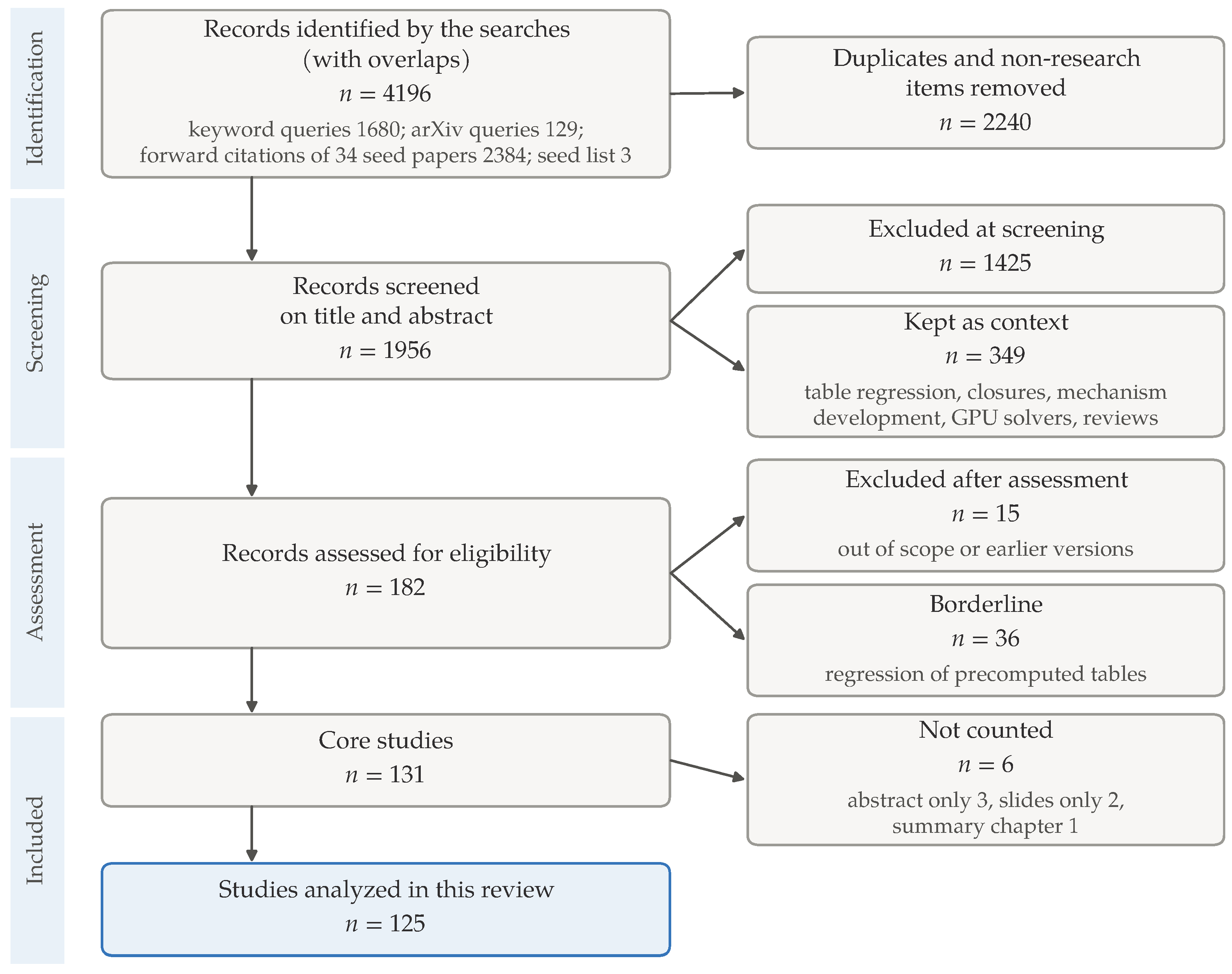
Each assessed record was assigned to one of three groups. Core studies use a network to represent or accelerate the integration of finite-rate chemistry; principal-component transport with source terms learned from finite-rate data counts as core, whereas networks that regress a manifold or table precomputed from canonical flamelets or homogeneous trajectories are borderline. The remaining records were excluded, including earlier versions of a study published again later. This gave 131 core, 36 borderline, and 15 excluded records. A record counts in the statistics if it is a core study, an original study (not a review or summary chapter), in English, and was read in full as a paper (not only as slides or an abstract): 125 studies. Of the core studies, 3 available only as abstracts, 2 available only as slides, and one summary chapter are listed in the evidence table but not counted. In the text, “the studies” means these 125 studies unless stated otherwise.
Appendix A.2. Extraction and Coding
For each record, a fixed set of fields was extracted from the full text: approach, architecture, inputs and outputs, fuel and mechanism, conditions, training data and training-set size, time step, constraints, a priori and a posteriori tests, platform, long-run behavior, minor species and pollutants, tests outside the training data, speedups with baseline, scope and hardware, and code and data. Each number was accompanied by a supporting quotation. Four codebooks then defined the categorical codes used for all counts: what the network gives the solver, its variables and time step, constraints, validation level, long-run evidence, transfer, NO and CO evidence, speedup comparisons and values, fallback, and code availability (codebook 2); training-data sources, the relation of training and tested cases, test splits, training-set size, constraint details, and conservation residuals (codebook 3); the combustion quantities compared a posteriori with their errors (codebook 4); and the physics of the tests, namely combustion regimes, configurations, flow and turbulence–chemistry models, species transport, differential diffusion, heat loss, walls, pressure, low-temperature chemistry, fuels, chemistry shares of the run time, and the explanations given by the authors (codebook 5). The previous reviews of Table S9 of the Supplementary Materials were coded with a separate codebook.
The supporting quotations were matched automatically against the full texts, and conflicting conventions between batches were harmonized by explicit rules and logged. In a second pass, a large language model checked every statement of the submitted version of this review that reports a result of a cited source against the full text of that source, quoting the passage and its location, and every statement that needed a change was corrected. The 9 statement–source pairs added in the revision were checked against the full texts in the same way, and the statements reworded in the revision were compared with their checked wording. Finally, the two authors checked by hand all 588 statement–source pairs, of the submitted version and of the revision, against the original papers, and the codes and speedup entries of all 182 rows of the evidence table, including the records not counted in the statistics, against their sources; they found no error. The data digitized from published figures, Figures 4b and 8a of Liu et al. [94] with Figures S6a, S9a, and S9c of its Supplementary Materials, and Figure 8a of Darzi et al. [27], were checked by overlaying them on the source figures. Figure 7b uses 8000 points of each digitized data set, drawn at random from 81,238 heat-sink, 20,786 free-flame, and 17,606 combustor points; the regions of the training flames are the highest-density regions holding 99% of these points, from a histogram smoothed with a Gaussian filter, and the combustor states with CO2 are drawn as points. The regions describe where the training states lie, not a strict boundary of their coverage. The coded table and its codebook are Table S3 of the Supplementary Materials; the verification records and the logs are available from the authors (Data Availability Statement).
Appendix A.3. Calculations with Cantera
The calculations of Section 2, Section 5, and Section 6 analyze idealized reactors and flames with published mechanisms, to quantify the requirements against which the reviewed studies are assessed. They used Cantera 3.2.0 [165] and air as 21% O2 and 79% N2 by volume. For methane, they used GRI-Mech 3.0 [166] as distributed with Cantera (53 species, 325 reactions); for hydrogen and ammonia/hydrogen (70/30 by volume), the mechanism of Stagni et al. [37] (31 species, 203 reactions) and, as a check at 1000 K, the H/O/N subset of the mechanism of Glarborg et al. [1] (31 species, 210 reactions). The autoignition of Figure 2 was computed in an adiabatic constant-pressure reactor with relative and absolute tolerances of and ; the ignition delay is the time of the largest . The Jacobian of Equation (1) in the variables was evaluated by central differences at 1262 states along the trajectory, spaced logarithmically in time and down to 0.02 µs apart around ignition, with relative perturbations of (at least K for the temperature and for the mass fractions), and its eigenvalues and eigenvectors were computed with NumPy; the CSP pointer of a mode is the element-wise product of its right and left eigenvectors [29]. The counterflow flames of Figure 3a, for methane and air at 300 K and 1 atm with unit Lewis numbers, were obtained by continuation in the strain rate with the scaling of the Cantera extinction example, from the lowest strain rate to the last burning solution; the strain rate is the largest axial velocity gradient. The equilibrium curves mix the two streams linearly in mass fractions and enthalpy; the enthalpy defect is a fraction of the sensible enthalpy of the adiabatic equilibrium products above 300 K, and the limit of complete combustion converts CH4 and O2 to CO2 and H2O at the mixture enthalpy. The premixed flames of Figure 3b (, 300 K, 1 atm) are freely propagating flames with mixture-averaged transport and with unit Lewis numbers, and burner-stabilized flames with mixture-averaged transport and mass fluxes of one half and one quarter of , all refined successively to about 3000 grid points, because, with first-order upwind convection, grids of about 200 points give flame speeds up to 1.6% higher; the mixtures of burned and unburned gas mix mass fractions and enthalpy linearly and take the temperature from the enthalpy. The sensitivity of thermal NO was computed from the initial net production rate of NO in the products of a mixture with at 10 bar, with all nitrogen species except N2 removed, at 1980, 2000, and 2020 K, either at the composition of 2000 K or with the composition brought to equilibrium at each temperature.
For Figure 4, the exact reaction map was the same reactor advanced over one time step and restarted at every step from the state returned by the previous step, with the prescribed error added. The step was 1 µs throughout; at equilibrium, the error was a bias of K per step in temperature and of per step in mass fraction moved from CO2 to H2O; the element balance was restored, where stated, by the smallest correction weighted by the mass fractions, and the temperature was computed, where stated, from the enthalpy, pressure, and composition. During the induction, an error was added per step to the mass fractions of H, O, and OH, and the ignition delay was taken as the time to a temperature rise of 400 K, interpolated within the step. After ignition, an error of a fixed fraction of the first NO increment was added to the NO mass fraction at every step from 20 ms to 0.6 s; a repetition at 10 µs gave the same relative errors.
For Figure 5 and Table 1, lean mixtures () were computed from 1000 to 1200 K and 1 to 20 bar (methane: 1100 and 1200 K, 5 to 20 bar) with additive errors of to per step in the mass fractions of H, O, and OH and with their increments over each step multiplied by , to 1, the temperature being kept when the mass fractions were reset. The bias for a 5% advance was interpolated logarithmically between the computed advances, and was obtained from the fit of Equation (4) and compared with the integral of the eigenvalue with the largest real part from 0 to , evaluated at 240 states of the reference trajectory. For the NO tolerance, the bias of the undamped estimate was added to the NO mass fraction at every step over 10 ms after , and the tolerance for 10% is this bias scaled by the ratio of 10% to the error it produced. The largest increments of NO and H2O per step during ignition are the changes of the exact map over one step. For hydrogen at 1000 K and 1 bar, 1100 K and 5 bar, and 1200 K and 5 and 10 bar, the response to a relative error and the bias for a 5% advance, with the same bias per unit time, were also computed at steps of 0.25 and 0.1 µs (Table S11 of the Supplementary Materials). The CSP pointer of the explosive mode, the mode of the eigenvalue with the largest real part, was evaluated at half the ignition delay.
Seven of these conditions were recomputed with an independent implementation of these definitions, with different integrator tolerances, one persistent reactor, and its own interpolation and fit. The delays, the bias tolerances, and the NO quantities, including the NO errors of the runs with a bias, agreed to four significant digits, the advances larger than 0.1% of the delay to three, and the delay changes for a relative error to within 0.001 percentage points. The smaller advances, which approach the accuracy of the integrators, differed by up to 34%. The fitted differed by up to 5%. The methane ignition delays from 1000 to 1400 K at 5, 10, and 20 bar with an error of per step are shown in Figure S6 of the Supplementary Materials.
For Figure 7, the heat release rate was evaluated at the states of a mixture-averaged free flame at the conditions of Figure 3b, solved on 953 grid points, at their own enthalpy and with their sensible enthalpy above 300 K reduced by 20% and 40% at fixed composition, with the temperature following from the reduced enthalpy.
The calculations behind Figure 2 and Figure 3 were repeated with a second, independent implementation of the definitions above, with different numerical choices: fourth-order differences that keep the mass fractions non-negative, checked against an analytical Jacobian, every integrator step as a state, and interpolated crossing times. The two scripts agree to within 0.3% on every recomputed number, with the flame speeds extrapolated to zero grid spacing; the largest difference is in the extinction strain rate of the counterflow flame, 2052 against 2046 s−1, which the two continuations approach in different steps.
Appendix A.4. Limitations
The counts are not weighted by the quality or size of a study: a conference paper and a journal article count once each. Restricting the set to the 87 journal articles changes the main proportions little; for example, 52% of them ran a network inside a flow solver (53% of all studies), and their median like-for-like chemistry speedup is 10 (10 for all studies). The codes record what a study reports, so a test that was done but not reported counts as not done. Some codes require judgment, notably the comparison behind a speedup and a test’s distance from the training data; their definitions are given in the codebooks. The search relied mainly on OpenAlex and likely missed conference papers without indexed abstracts; theses were excluded by design.
Appendix A.5. Relation to Previous Reviews
To define what previous reviews of machine learning in combustion cover, the thirteen reviews closest to this topic were coded from their full texts with the same questions as the primary studies (Table S9 of the Supplementary Materials). Most of them describe the methods study by study and cite between 3 and 38 studies of neural-network chemistry. Several discuss constraints and tests outside the training data, whereas only one recent preprint treats error accumulation over long runs in a paragraph or more, none treats slow species, and only two treat the comparison behind reported speedups or reporting standards. Shateri et al. synthesize 125 surrogate studies across all scales of combustion and propose minimum reporting requirements for chemistry surrogates, including a defined baseline with mechanism size, solver tolerances, and hardware, and separate training, inference, and end-to-end timings [18]. Mirgolbabaei grades the evidence for data-driven low-dimensional manifold models, of which about 14 cited studies concern network chemistry as defined here, and proposes a reporting standard [19].
References
- Glarborg, P.; Miller, J.A.; Ruscic, B.; Klippenstein, S.J. Modeling nitrogen chemistry in combustion. Prog. Energy Combust. Sci. 2018, 67, 31–68. [Google Scholar] [CrossRef] [Scilit]
- Pope, S.B. Small scales, many species and the manifold challenges of turbulent combustion. Proc. Combust. Inst. 2013, 34, 1–31. [Google Scholar] [CrossRef] [Scilit]
- Lu, T.; Law, C.K. Toward accommodating realistic fuel chemistry in large-scale computations. Prog. Energy Combust. Sci. 2009, 35, 192–215. [Google Scholar] [CrossRef] [Scilit]
- Pope, S. Computationally efficient implementation of combustion chemistry using in situ adaptive tabulation. Combust. Theory Model. 1997, 1, 41–63. [Google Scholar] [CrossRef] [Scilit]
- Hindmarsh, A.C.; Brown, P.N.; Grant, K.E.; Lee, S.L.; Serban, R.; Shumaker, D.E.; Woodward, C.S. SUNDIALS: Suite of nonlinear and differential/algebraic equation solvers. ACM Trans. Math. Softw. 2005, 31, 363–396. [Google Scholar] [CrossRef] [Scilit]
- Perini, F.; Galligani, E.; Reitz, R.D. An Analytical Jacobian Approach to Sparse Reaction Kinetics for Computationally Efficient Combustion Modeling with Large Reaction Mechanisms. Energy Fuels 2012, 26, 4804–4822. [Google Scholar] [CrossRef] [Scilit]
- Curtis, N.J.; Niemeyer, K.E.; Sung, C.J. An investigation of GPU-based stiff chemical kinetics integration methods. Combust. Flame 2017, 179, 312–324. [Google Scholar] [CrossRef] [Scilit]
- Cai, Y.; Ban, Y.; Dang, G.; Gong, T.; Wang, H.; Zhang, F.; Chen, Z.X. A GPU-accelerated stiff ODE solver for combustion CFD with fully analytical chemical kinetics and heterogeneous CPU/GPU integration. Fuel 2026, 408, 137627. [Google Scholar] [CrossRef] [Scilit]
- Christo, F.; Masri, A.; Nebot, E.; Turanyi, T. Utilising artificial neural network and repro-modelling in turbulent combustion. In Proceedings of the ICNN’95—International Conference on Neural Networks; IEEE: New York, NY, USA, 1995; Volume 2, ICNN-95, pp. 911–916. [Google Scholar] [CrossRef] [Scilit]
- Christo, F.; Masri, A.; Nebot, E.; Pope, S. An integrated PDF/neural network approach for simulating turbulent reacting systems. Symp. (Int.) Combust. 1996, 26, 43–48. [Google Scholar] [CrossRef] [Scilit]
- Blasco, J.; Fueyo, N.; Dopazo, C.; Ballester, J. Modelling the Temporal Evolution of a Reduced Combustion Chemical System With an Artificial Neural Network. Combust. Flame 1998, 113, 38–52. [Google Scholar] [CrossRef] [Scilit]
- Mao, R.; Lin, M.; Zhang, Y.; Zhang, T.; Xu, Z.Q.J.; Chen, Z.X. DeepFlame: A deep learning empowered open-source platform for reacting flow simulations. Comput. Phys. Commun. 2023, 291, 108842. [Google Scholar] [CrossRef] [Scilit]
- Li, H.; Xiao, K.; Xu, Y.; Zhang, H.; Chen, Z.; Mao, R.; Chen, Z.X. DFODE-Kit: Deep learning package for solving flame chemical kinetics with high-dimensional stiff ordinary differential equations. Comput. Phys. Commun. 2026, 321, 110013. [Google Scholar] [CrossRef] [Scilit]
- Guo, Z.; Mao, R.; Liu, L.; Tan, G.; Jia, W.; Chen, Z.X. Deep Learning-Enabled Supercritical Flame Simulation at Detailed Chemistry and Real-Fluid Accuracy Towards Trillion-Cell Scale. In Proceedings of the SC ’25, International Conference for High Performance Computing, Networking, Storage and Analysis; ACM: New York, NY, USA, 2025; pp. 1888–1900. [Google Scholar] [CrossRef] [Scilit]
- Zhou, L.; Song, Y.; Ji, W.; Wei, H. Machine learning for combustion. Energy AI 2022, 7, 100128. [Google Scholar] [CrossRef] [Scilit]
- Ihme, M.; Chung, W.T.; Mishra, A.A. Combustion machine learning: Principles, progress and prospects. Prog. Energy Combust. Sci. 2022, 91, 101010. [Google Scholar] [CrossRef] [Scilit]
- Echekki, T.; Farooq, A.; Ihme, M.; Sarathy, S.M. Machine Learning for Combustion Chemistry. In Machine Learning and Its Application to Reacting Flows; Springer International Publishing: Cham, Switzerland, 2023; pp. 117–147. [Google Scholar] [CrossRef] [Scilit]
- Shateri, A.; Yang, Z.; Yan, Y.; Paul, M.C.; Xie, J. AI-Powered Surrogate Modelling for Multiscale Combustion: A Critical Review and Opportunities. arXiv 2026. [Google Scholar] [CrossRef] [Scilit]
- Mirgolbabaei, H. The Evolution of Data-Driven Low-Dimensional Manifolds for Combustion: From Canonical Flames to Biofuels. Preprints 2026. [Google Scholar] [CrossRef] [Scilit]
- Ren, Z.; Pope, S.B. Second-order splitting schemes for a class of reactive systems. J. Comput. Phys. 2008, 227, 8165–8176. [Google Scholar] [CrossRef] [Scilit]
- Haworth, D. Progress in probability density function methods for turbulent reacting flows. Prog. Energy Combust. Sci. 2010, 36, 168–259. [Google Scholar] [CrossRef] [Scilit]
- Valiño, L. A Field Monte Carlo Formulation for Calculating the Probability Density Function of a Single Scalar in a Turbulent Flow. Flow Turbul. Combust. 1998, 60, 157–172. [Google Scholar] [CrossRef] [Scilit]
- JONES, W.; NAVARROMARTINEZ, S. Large eddy simulation of autoignition with a subgrid probability density function method. Combust. Flame 2007, 150, 170–187. [Google Scholar] [CrossRef] [Scilit]
- Day, M.S.; Bell, J.B. Numerical simulation of laminar reacting flows with complex chemistry. Combust. Theory Model. 2000, 4, 535–556. [Google Scholar] [CrossRef] [Scilit]
- Chen, J.H.; Choudhary, A.; de Supinski, B.; DeVries, M.; Hawkes, E.R.; Klasky, S.; Liao, W.K.; Ma, K.L.; Mellor-Crummey, J.; Podhorszki, N.; et al. Terascale direct numerical simulations of turbulent combustion using S3D. Comput. Sci. Discov. 2009, 2, 015001. [Google Scholar] [CrossRef] [Scilit]
- Zhang, M.; Dang, G.; Mao, R.; Cai, Y.; Yang, R.; Li, H.; Chen, Z.X. Performance comparison of machine learning and GPU accelerated solvers in high-fidelity simulation of Cambridge stratified flames. Fuel 2026, 426, 139562. [Google Scholar] [CrossRef] [Scilit]
- Darzi, A.; Jones, W.; Rigopoulos, S. Machine learning tabulation of thermochemistry: Transfer learning for non-adiabatic flames. Energy AI 2026, 24, 100746. [Google Scholar] [CrossRef] [Scilit]
- Hairer, E.; Wanner, G. Solving Ordinary Differential Equations II; Springer: Berlin/Heidelberg, Germany, 1996. [Google Scholar] [CrossRef] [Scilit]
- Lam, S.H.; Goussis, D.A. The CSP method for simplifying kinetics. Int. J. Chem. Kinet. 1994, 26, 461–486. [Google Scholar] [CrossRef] [Scilit]
- Maas, U.; Pope, S. Simplifying chemical kinetics: Intrinsic low-dimensional manifolds in composition space. Combust. Flame 1992, 88, 239–264. [Google Scholar] [CrossRef] [Scilit]
- LU, T.F.; YOO, C.S.; CHEN, J.H.; LAW, C.K. Three-dimensional direct numerical simulation of a turbulent lifted hydrogen jet flame in heated coflow: A chemical explosive mode analysis. J. Fluid Mech. 2010, 652, 45–64. [Google Scholar] [CrossRef] [Scilit]
- Wu, W.; Piao, Y.; Xie, Q.; Ren, Z. Flame Diagnostics with a Conservative Representation of Chemical Explosive Mode Analysis. AIAA J. 2019, 57, 1355–1363. [Google Scholar] [CrossRef] [Scilit]
- Sen, B.A.; Menon, S. Linear eddy mixing based tabulation and artificial neural networks for large eddy simulations of turbulent flames. Combust. Flame 2010, 157, 62–74. [Google Scholar] [CrossRef] [Scilit]
- Laubscher, R. Utilization of basic multi-layer perceptron artificial neural networks to resolve turbulent fine structure chemical kinetics applied to a CFD model of a methane/air piloted jet flame. J. Therm. Eng. 2018, 4, 1828–1846. [Google Scholar] [CrossRef] [Scilit]
- Reiter, T.; Volgger, J.; Früh, M.; Hochenauer, C.; Prieler, R. RANS Simulation of Turbulent Flames Under Different Operating Conditions Using Artificial Neural Networks for Accelerating Chemistry Modeling. Processes 2025, 13, 2220. [Google Scholar] [CrossRef] [Scilit]
- Ukorigho, O.; Owoyele, O. Entropy-constrained machine learning with residual data augmentation for modeling chemical kinetics. Proc. Combust. Inst. 2026, 42, 106456. [Google Scholar] [CrossRef] [Scilit]
- Stagni, A.; Arunthanayothin, S.; Dehue, M.; Herbinet, O.; Battin-Leclerc, F.; Bréquigny, P.; Mounaïm-Rousselle, C.; Faravelli, T. Low- and intermediate-temperature ammonia/hydrogen oxidation in a flow reactor: Experiments and a wide-range kinetic modeling. Chem. Eng. J. 2023, 471, 144577. [Google Scholar] [CrossRef] [Scilit]
- Law, C.K. Combustion Physics; Cambridge University Press: Cambridge, UK, 2006. [Google Scholar] [CrossRef] [Scilit]
- Li, H.; Yang, R.; Xu, Y.; Zhang, M.; Mao, R.; Chen, Z.X. Comprehensive deep learning for combustion chemistry integration: Multi-fuel generalization and a posteriori validation in reacting flow. Phys. Fluids 2025, 37, 015162. [Google Scholar] [CrossRef] [Scilit]
- Lu, T.; Law, C.K. A directed relation graph method for mechanism reduction. Proc. Combust. Inst. 2005, 30, 1333–1341. [Google Scholar] [CrossRef] [Scilit]
- PEPIOTDESJARDINS, P.; PITSCH, H. An efficient error-propagation-based reduction method for large chemical kinetic mechanisms. Combust. Flame 2008, 154, 67–81. [Google Scholar] [CrossRef] [Scilit]
- Keck, J.C. Rate-controlled constrained-equilibrium theory of chemical reactions in complex systems. Prog. Energy Combust. Sci. 1990, 16, 125–154. [Google Scholar] [CrossRef] [Scilit]
- Liang, L.; Stevens, J.G.; Farrell, J.T. A dynamic adaptive chemistry scheme for reactive flow computations. Proc. Combust. Inst. 2009, 32, 527–534. [Google Scholar] [CrossRef] [Scilit]
- Contino, F.; Jeanmart, H.; Lucchini, T.; D’Errico, G. Coupling of in situ adaptive tabulation and dynamic adaptive chemistry: An effective method for solving combustion in engine simulations. Proc. Combust. Inst. 2011, 33, 3057–3064. [Google Scholar] [CrossRef] [Scilit]
- Turányi, T.; Tomlin, A.S. Analysis of Kinetic Reaction Mechanisms; Springer: Berlin/Heidelberg, Germany, 2014. [Google Scholar] [CrossRef] [Scilit]
- OIJEN, J.V.; GOEY, L.D. Modelling of Premixed Laminar Flames using Flamelet-Generated Manifolds. Combust. Sci. Technol. 2000, 161, 113–137. [Google Scholar] [CrossRef] [Scilit]
- PIERCE, C.D.; MOIN, P. Progress-variable approach for large-eddy simulation of non-premixed turbulent combustion. J. Fluid Mech. 2004, 504, 73–97. [Google Scholar] [CrossRef] [Scilit]
- Turányi, T. Parameterization of reaction mechanisms using orthonormal polynomials. Comput. Chem. 1994, 18, 45–54. [Google Scholar] [CrossRef] [Scilit]
- Tonse, S.R.; Moriarty, N.W.; Brown, N.J.; Frenklach, M. PRISM: Piecewise Reusable Implementation of Solution Mapping. An Economical Strategy for Chemical Kinetics. Isr. J. Chem. 1999, 39, 97–106. [Google Scholar] [CrossRef] [Scilit]
- Chen, J.Y.; Blasco, J.; Fueyo, N.; Dopazo, C. An economical strategy for storage of chemical kinetics: Fitting in situ adaptive tabulation with artificial neural networks. Proc. Combust. Inst. 2000, 28, 115–121. [Google Scholar] [CrossRef] [Scilit]
- Niemeyer, K.E.; Curtis, N.J.; Sung, C.J. pyJac: Analytical Jacobian generator for chemical kinetics. Comput. Phys. Commun. 2017, 215, 188–203. [Google Scholar] [CrossRef] [Scilit]
- Shi, Y.; Green, W.H.; Wong, H.W.; Oluwole, O.O. Redesigning combustion modeling algorithms for the Graphics Processing Unit (GPU): Chemical kinetic rate evaluation and ordinary differential equation integration. Combust. Flame 2011, 158, 836–847. [Google Scholar] [CrossRef] [Scilit]
- Niemeyer, K.E.; Sung, C.J. Accelerating moderately stiff chemical kinetics in reactive-flow simulations using GPUs. J. Comput. Phys. 2014, 256, 854–871. [Google Scholar] [CrossRef] [Scilit]
- Sewerin, F.; Rigopoulos, S. A methodology for the integration of stiff chemical kinetics on GPUs. Combust. Flame 2015, 162, 1375–1394. [Google Scholar] [CrossRef] [Scilit]
- Stone, C.P.; Alferman, A.T.; Niemeyer, K.E. Accelerating finite-rate chemical kinetics with coprocessors: Comparing vectorization methods on GPUs, MICs, and CPUs. Comput. Phys. Commun. 2018, 226, 18–29. [Google Scholar] [CrossRef] [Scilit]
- Hernández Pérez, F.E.; Mukhadiyev, N.; Xu, X.; Sow, A.; Lee, B.J.; Sankaran, R.; Im, H.G. Direct numerical simulations of reacting flows with detailed chemistry using many-core/GPU acceleration. Comput. Fluids 2018, 173, 73–79. [Google Scholar] [CrossRef] [Scilit]
- Barwey, S.; Raman, V. A Neural Network-Inspired Matrix Formulation of Chemical Kinetics for Acceleration on GPUs. Energies 2021, 14, 2710. [Google Scholar] [CrossRef] [Scilit]
- Uranakara, H.A.; Barwey, S.; Hernández Pérez, F.E.; Vijayarangan, V.; Raman, V.; Im, H.G. Accelerating turbulent reacting flow simulations on many-core/GPUs using matrix-based kinetics. Proc. Combust. Inst. 2023, 39, 5127–5136. [Google Scholar] [CrossRef] [Scilit]
- Christo, F. Artificial neural network implementation of chemistry with pdf simulation of H2/CO2 flames. Combust. Flame 1996, 106, 406–427. [Google Scholar] [CrossRef] [Scilit]
- Blasco, J.; Fueyo, N.; Larroya, J.; Dopazo, C.; Chen, Y.J. A single-step time-integrator of a methane–air chemical system using artificial neural networks. Comput. Chem. Eng. 1999, 23, 1127–1133. [Google Scholar] [CrossRef] [Scilit]
- Blasco, J.; Fueyo, N.; Dopazo, C.; Chen, J.Y. A self-organizing-map approach to chemistry representation in combustion applications. Combust. Theory Model. 2000, 4, 61–76. [Google Scholar] [CrossRef] [Scilit]
- Ihme, M.; Schmitt, C.; Pitsch, H. Optimal artificial neural networks and tabulation methods for chemistry representation in LES of a bluff-body swirl-stabilized flame. Proc. Combust. Inst. 2009, 32, 1527–1535. [Google Scholar] [CrossRef] [Scilit]
- Sen, B.; Menon, S. Representation of Chemical Kinetics by Artificial Neural Networks for Large Eddy Simulations. In Proceedings of the 43rd AIAA/ASME/SAE/ASEE Joint Propulsion Conference & Exhibit; American Institute of Aeronautics and Astronautics: Reston, VA, USA, 2007. [Google Scholar] [CrossRef] [Scilit]
- Sen, B.A.; Menon, S. Turbulent premixed flame modeling using artificial neural networks based chemical kinetics. Proc. Combust. Inst. 2009, 32, 1605–1611. [Google Scholar] [CrossRef] [Scilit]
- Sen, B.; Menon, S. Artificial Neural Networks Based Chemistry-Mixing Subgrid Model for LES. In Proceedings of the 47th AIAA Aerospace Sciences Meeting including The New Horizons Forum and Aerospace Exposition; American Institute of Aeronautics and Astronautics: Reston, VA, USA, 2009. [Google Scholar] [CrossRef] [Scilit]
- Sen, B.A.; Hawkes, E.R.; Menon, S. Large eddy simulation of extinction and reignition with artificial neural networks based chemical kinetics. Combust. Flame 2010, 157, 566–578. [Google Scholar] [CrossRef] [Scilit]
- Sinaei, P.; Tabejamaat, S. Large eddy simulation of methane diffusion jet flame with representation of chemical kinetics using artificial neural network. Proc. Inst. Mech. Eng. Part E J. Process. Mech. Eng. 2016, 231, 147–163. [Google Scholar] [CrossRef] [Scilit]
- Chatzopoulos, A.; Rigopoulos, S. A chemistry tabulation approach via Rate-Controlled Constrained Equilibrium (RCCE) and Artificial Neural Networks (ANNs), with application to turbulent non-premixed CH4/H2/N2 flames. Proc. Combust. Inst. 2013, 34, 1465–1473. [Google Scholar] [CrossRef] [Scilit]
- Franke, L.L.; Chatzopoulos, A.K.; Rigopoulos, S. Tabulation of combustion chemistry via Artificial Neural Networks (ANNs): Methodology and application to LES-PDF simulation of Sydney flame L. Combust. Flame 2017, 185, 245–260. [Google Scholar] [CrossRef] [Scilit]
- Mirgolbabaei, H.; Echekki, T. A novel principal component analysis-based acceleration scheme for LES–ODT: An a priori study. Combust. Flame 2013, 160, 898–908. [Google Scholar] [CrossRef] [Scilit]
- Echekki, T.; Mirgolbabaei, H. Principal component transport in turbulent combustion: A posteriori analysis. Combust. Flame 2015, 162, 1919–1933. [Google Scholar] [CrossRef] [Scilit]
- Owoyele, O.; Echekki, T. Toward computationally efficient combustion DNS with complex fuels via principal component transport. Combust. Theory Model. 2017, 21, 770–798. [Google Scholar] [CrossRef] [Scilit]
- Ding, T.; Readshaw, T.; Rigopoulos, S.; Jones, W. Machine learning tabulation of thermochemistry in turbulent combustion: An approach based on hybrid flamelet/random data and multiple multilayer perceptrons. Combust. Flame 2021, 231, 111493. [Google Scholar] [CrossRef] [Scilit]
- Zhang, T.; Yi, Y.; Xu, Y.; Chen, Z.X.; Zhang, Y.; E, W.; Xu, Z.Q.J. A multi-scale sampling method for accurate and robust deep neural network to predict combustion chemical kinetics. Combust. Flame 2022, 245, 112319. [Google Scholar] [CrossRef] [Scilit]
- Wang, T.; Yi, Y.; Yao, J.; Xu, Z.Q.J.; Zhang, T.; Chen, Z. Enforcing physical conservation in neural network surrogate models for complex chemical kinetics. Combust. Flame 2025, 275, 114105. [Google Scholar] [CrossRef] [Scilit]
- Owoyele, O.; Pal, P. ChemNODE: A neural ordinary differential equations framework for efficient chemical kinetic solvers. Energy AI 2022, 7, 100118. [Google Scholar] [CrossRef] [Scilit]
- Koenig, B.C.; Kim, S.; Deng, S. ChemKANs for combustion chemistry modeling and acceleration. Phys. Chem. Chem. Phys. 2025, 27, 17313–17330. [Google Scholar] [CrossRef] [Scilit] [PubMed]
- Goswami, S.; Jagtap, A.D.; Babaee, H.; Susi, B.T.; Karniadakis, G.E. Learning stiff chemical kinetics using extended deep neural operators. Comput. Methods Appl. Mech. Eng. 2024, 419, 116674. [Google Scholar] [CrossRef] [Scilit]
- Jo, J.; Kang, K.; Wiersema, P.; Yoo, J.; Mayhew, E.; Lee, T. Fast and accurate prediction of H 2 combustion via data-augmented physics-informed operator learning. Eng. Appl. Artif. Intell. 2025, 160, 111850. [Google Scholar] [CrossRef] [Scilit]
- Nath, K.; Pandey, A.; Susi, B.T.; Babaee, H.; Karniadakis, G.E. AMORE: Adaptive multi-output operator network for stiff chemical kinetics. J. Comput. Phys. 2026, 562, 115030. [Google Scholar] [CrossRef] [Scilit]
- Babić, M.; Rohrhofer, F.M.; Posch, S. Differentiable Chemistry in PINNs for Solving Parameterized and Stiff Reaction Systems. arXiv 2026. [Google Scholar] [CrossRef] [Scilit]
- Lapointe, S.; Mondal, S.; Whitesides, R.A. Data-driven selection of stiff chemistry ODE solver in operator-splitting schemes. Combust. Flame 2020, 220, 133–143. [Google Scholar] [CrossRef] [Scilit]
- D’Alessio, G.; Cuoci, A.; Parente, A. Feature extraction and artificial neural networks for the on-the-fly classification of high-dimensional thermochemical spaces in adaptive-chemistry simulations. Data-Centric Eng. 2021, 2, e2. [Google Scholar] [CrossRef] [Scilit]
- Kim, M.H.; Mo, H.S.; Lacey, C.E.; Jung, K.S.; Chen, J.H.; Yoo, C.S. MG-ANN: An online extension of reduced-order modeling with continual learning for turbulent reacting flows. Proc. Combust. Inst. 2026, 42, 106546. [Google Scholar] [CrossRef] [Scilit]
- Mishra, R.; Mousavi, M.; Nelson, A.; Jarrahbashi, D. Supervised learning-adaptive global pathway selection method coupled with in-situ adaptive tabulation to accelerate reacting simulations. Fuel 2026, 415, 138379. [Google Scholar] [CrossRef] [Scilit]
- Zhang, Y.; Du, W. Intelligent Time-Scale Operator-Splitting Integration for Chemical Reaction Systems. IEEE Trans. Neural Netw. Learn. Syst. 2021, 32, 3366–3376. [Google Scholar] [CrossRef] [Scilit] [PubMed]
- Chi, C.; Janiga, G.; Thévenin, D. On-the-fly artificial neural network for chemical kinetics in direct numerical simulations of premixed combustion. Combust. Flame 2021, 226, 467–477. [Google Scholar] [CrossRef] [Scilit]
- Mehl, C.; Aubagnac-Karkar, D. On-the-fly accuracy evaluation of artificial neural networks and hybrid method to improve the robustness of neural network accelerated chemistry solving. Phys. Fluids 2023, 35, 067115. [Google Scholar] [CrossRef] [Scilit]
- Jo, J.; Kang, K.; Mayhew, E.; Yoo, J.; Lee, T. Deep operator network enabled CFD framework for accelerating finite-rate stiff combustion chemistry. SSRN Prepr. 2026. [Google Scholar] [CrossRef] [Scilit]
- Zhang, P.; Chindada, S.; Duwig, C. Reduced-chemistry LES of hydrogen combustion using neural-network-based NO source-term prediction. SSRN Prepr. 2026. [Google Scholar] [CrossRef] [Scilit]
- Zhang, S.; Zhang, C.; Wang, B. CRK-PINN: A physics-informed neural network for solving combustion reaction kinetics ordinary differential equations. Combust. Flame 2024, 269, 113647. [Google Scholar] [CrossRef] [Scilit]
- Amarathunga, D.V.; Echekki, T. React-NIF: A neural implicit flow-based framework for complex fuel combustion chemistry acceleration. Fuel 2026, 412, 138166. [Google Scholar] [CrossRef] [Scilit]
- Nguyen, H.T.; Domingo, P.; Vervisch, L.; Nguyen, P.D. Machine learning for integrating combustion chemistry in numerical simulations. Energy AI 2021, 5, 100082. [Google Scholar] [CrossRef] [Scilit]
- Liu, W.; Kronenburg, A.; Zirwes, T. A randomization and unrolling framework to improve deep neural networks modelling chemistry integration across multiple combustion regimes. Appl. Energy Combust. Sci. 2026, 25, 100445. [Google Scholar] [CrossRef] [Scilit]
- Akeweje, E.; Vanovskiy, V.; Vishnyakov, A. Surrogate Models of Hydrogen Oxidation Kinetics based on Deep Neural Networks. Theor. Found. Chem. Eng. 2023, 57, 196–204. [Google Scholar] [CrossRef] [Scilit]
- Kumar, A.; Echekki, T. Combustion chemistry acceleration with DeepONets. Fuel 2024, 365, 131212. [Google Scholar] [CrossRef] [Scilit]
- Weng, Y.; Li, H.; Zhang, H.; Chen, Z.X.; Zhou, D. Extended Fourier Neural Operators to learn stiff chemical kinetics under unseen conditions. Combust. Flame 2025, 272, 113847. [Google Scholar] [CrossRef] [Scilit]
- Liu, Z.; Ma, H.; Wang, H.; Liu, J.; Zeng, W. Ms-CRK-PINN:A Multi-Step Physics-Informed Neural Network for Surrogate Modeling and Acceleration of RP-3 Aviation Kerosene Combustion Kinetics. SSRN Prepr. 2026. [Google Scholar] [CrossRef] [Scilit]
- Ji, W.; Qiu, W.; Shi, Z.; Pan, S.; Deng, S. Stiff-PINN: Physics-Informed Neural Network for Stiff Chemical Kinetics. J. Phys. Chem. 2021, 125, 8098–8106. [Google Scholar] [CrossRef] [Scilit] [PubMed]
- Bansude, S.; Imani, F.; Sheikhi, R. A Data-Driven Framework for Computationally Efficient Integration of Chemical Kinetics Using Neural Ordinary Differential Equations. ASME Open J. Eng. 2023, 2, 021022. [Google Scholar] [CrossRef] [Scilit]
- Kumar, T.; Kumar, A.; Pal, P. A physics-constrained neural ordinary differential equations approach for robust learning of stiff chemical kinetics. Combust. Theory Model. 2025, 29, 332–347. [Google Scholar] [CrossRef] [Scilit]
- Dikeman, H.E.; Zhang, H.; Yang, S. Stiffness-Reduced Neural ODE Models for Data-Driven Reduced-Order Modeling of Combustion Chemical Kinetics. In Proceedings of the AIAA SCITECH 2022 Forum; American Institute of Aeronautics and Astronautics: Reston, VA, USA, 2022. [Google Scholar] [CrossRef] [Scilit]
- Vijayarangan, V.; Uranakara, H.A.; Barwey, S.; Galassi, R.M.; Malik, M.R.; Valorani, M.; Raman, V.; Im, H.G. A data-driven reduced-order model for stiff chemical kinetics using dynamics-informed training. Energy AI 2024, 15, 100325. [Google Scholar] [CrossRef] [Scilit]
- Kumar, T.; Kumar, A.; Pal, P. Phy-ChemNODE: An end-to-end physics-constrained autoencoder-NeuralODE framework for learning stiff chemical kinetics of hydrocarbon fuels. Front. Therm. Eng. 2025, 5, 1594443. [Google Scholar] [CrossRef] [Scilit]
- Vijayarangan, V.; Uranakara, H.A.; Hernández-Pérez, F.E.; Im, H.G. Understanding the role of autoencoders for stiff dynamical systems using information theory. Energy AI 2025, 21, 100567. [Google Scholar] [CrossRef] [Scilit]
- Saito, M.; Xing, J.; Nagao, J.; Kurose, R. Data-driven simulation of ammonia combustion using neural ordinary differential equations (NODE). Appl. Energy Combust. Sci. 2023, 16, 100196. [Google Scholar] [CrossRef] [Scilit]
- Wan, K.; Barnaud, C.; Vervisch, L.; Domingo, P. Chemistry reduction using machine learning trained from non-premixed micro-mixing modeling: Application to DNS of a syngas turbulent oxy-flame with side-wall effects. Combust. Flame 2020, 220, 119–129. [Google Scholar] [CrossRef] [Scilit]
- Cai, Y.; Yang, R.; Li, H.; Xu, J.; Xiao, K.; Chen, Z.X.; Wang, H. Efficient machine learning method for supercritical combustion: Predicting real-fluid properties and chemical ODEs. Aerosp. Sci. Technol. 2025, 159, 110034. [Google Scholar] [CrossRef] [Scilit]
- Xiao, K.; Xu, Y.; Li, H.; Chen, Z.X. Enhancing deep learning of ammonia/natural gas combustion kinetics via physics-aware data augmentation and scale separation. Fuel 2026, 419, 138904. [Google Scholar] [CrossRef] [Scilit]
- Weng, Y.; Li, H.; Li, K.; Chen, Z.X.; Zhou, D.; Lu, X. A Stiff Chemical Kinetics Solver based on Neural Network Models Trained by Low-Dimensional Generative Adversarial Network-augmented Data. SSRN Prepr. 2026. [Google Scholar] [CrossRef] [Scilit]
- Baykan, M.Y.; Vijayarangan, V.; Shin, D.h.; Im, H.G. Accelerated integration of stiff reactive systems using gradient-informed autoencoder and neural ordinary differential equation. Combust. Theory Model. 2025, 29, 783–814. [Google Scholar] [CrossRef] [Scilit]
- Wu, S.; Liang, W.; Luo, K.H. Deep learning based combustion chemistry acceleration method for widely applicable NH3/H2 turbulent combustion simulations. Combust. Flame 2025, 278, 114218. [Google Scholar] [CrossRef] [Scilit]
- Sharma, A.J.; Johnson, R.F.; Kessler, D.A.; Moses, A. Deep Learning for Scalable Chemical Kinetics. In Proceedings of the AIAA Scitech 2020 Forum; American Institute of Aeronautics and Astronautics, 2020. [Google Scholar] [CrossRef] [Scilit]
- Dalakoti, D.K.; Wehrfritz, A.; Savard, B.; Day, M.S.; Bell, J.B.; Hawkes, E.R. An a priori evaluation of a principal component and artificial neural network based combustion model in diesel engine conditions. Proc. Combust. Inst. 2021, 38, 2701–2709. [Google Scholar] [CrossRef] [Scilit]
- Béroudiaux, A.; Vervisch, L.; Domingo, P. Artificial neural network chemistry solving for high-pressure hydrogen–air combustion. Int. J. Hydrogen Energy 2025, 109, 669–683. [Google Scholar] [CrossRef] [Scilit]
- Li, H.; Yang, R.; Zhang, M.; Mao, R.; Chen, Z.X. A comprehensive study on the accuracy and generalization of deep learning-generated chemical ODE integrators. arXiv 2023. [Google Scholar] [CrossRef] [Scilit]
- Zhang, M.; Mao, R.; Li, H.; An, Z.; Chen, Z.X. Graphics processing unit/artificial neural network-accelerated large-eddy simulation of swirling premixed flames. Phys. Fluids 2024, 36, 055147. [Google Scholar] [CrossRef] [Scilit]
- Üstün, C.E.; Paykani, A. On-the-fly uncertainty-aware deep ensembles for stiff chemical kinetics. Proc. Combust. Inst. 2025, 41, 105896. [Google Scholar] [CrossRef] [Scilit]
- Readshaw, T.; Jones, W.P.; Rigopoulos, S. On the incorporation of conservation laws in machine learning tabulation of kinetics for reacting flow simulation. Phys. Fluids 2023, 35, 047103. [Google Scholar] [CrossRef] [Scilit]
- Pandey, A.; Wei, L.; Babaee, H.; Karniadakis, G.E. Kinetic-Mamba: Mamba-Assisted Predictions of Stiff Chemical Kinetics. J. Mach. Learn. Model. Comput. 2026, in press. [Google Scholar] [CrossRef] [Scilit]
- Readshaw, T.; Ding, T.; Rigopoulos, S.; Jones, W.P. Modeling of turbulent flames with the large eddy simulation–probability density function (LES–PDF) approach, stochastic fields, and artificial neural networks. Phys. Fluids 2021, 33, 035154. [Google Scholar] [CrossRef] [Scilit]
- Yi, Y.; Wang, W.; Zhang, T.; Xu, Z.Q.J. An output scaling layer boosts deep neural networks for multiscale ODE systems. arXiv 2025. [Google Scholar] [CrossRef] [Scilit]
- Ding, T.; Jones, W.; Rigopoulos, S. An improved machine learning method for thermochemistry tabulation, with application to LES-PDF simulations of piloted diffusion and swirl-bluff-body stabilised flames with NOx formation. Combust. Flame 2025, 277, 114130. [Google Scholar] [CrossRef] [Scilit]
- Mehl, C.; Aubagnac-Karkar, D. Simulation of reacting flows using artificial neural networks: Application to multi-regime combustion. In Proceedings of the 8th European Congress on Computational Methods in Applied Sciences and Engineering. CIMNE, 2022, ECCOMAS Congress 2022, Oslo, Norway, 5–9 June 2022. [Google Scholar] [CrossRef] [Scilit]
- Jung, K.S.; Kumar, A.; Echekki, T.; Chen, J.H. On the application of principal component transport for compression ignition of lean fuel/air mixtures under engine relevant conditions. Combust. Flame 2024, 260, 113204. [Google Scholar] [CrossRef] [Scilit]
- Son, G.H.; Park, H.R.; Jung, K.S. An assessment of the coupling between principal component analysis and nonlinear transformation in data-driven reduced-order models for combustion simulations. Combust. Flame 2026, 294, 115295. [Google Scholar] [CrossRef] [Scilit]
- Jung, K.S.; Echekki, T.; Chen, J.H.; Khalil, M. Transfer learning for predicting source terms of principal component transport in chemically reactive flow. Data-Centric Eng. 2024, 5, e42. [Google Scholar] [CrossRef] [Scilit]
- Han, X.; Jia, M.; Chang, Y.; Li, Y. An improved approach towards more robust deep learning models for chemical kinetics. Combust. Flame 2022, 238, 111934. [Google Scholar] [CrossRef] [Scilit]
- Haghshenas, M.; Mitra, P.; Santo, N.D.; Schmidt, D.P. Acceleration of Chemical Kinetics Computation with the Learned Intelligent Tabulation (LIT) Method. Energies 2021, 14, 7851. [Google Scholar] [CrossRef] [Scilit]
- Zhang, T.; Zhang, Y.; E, W.; Ju, Y. DLODE: A deep learning-based ODE solver for chemistry kinetics. In Proceedings of the AIAA Scitech 2021 Forum; American Institute of Aeronautics and Astronautics: Reston, VA, USA, 2021. [Google Scholar] [CrossRef] [Scilit]
- Alqahtani, S.; Gitushi, K.M.; Echekki, T. A Data-Based Hybrid Chemistry Acceleration Framework for the Low-Temperature Oxidation of Complex Fuels. Energies 2024, 17, 734. [Google Scholar] [CrossRef] [Scilit]
- Ding, T.; Rigopoulos, S.; Jones, W. Machine learning tabulation of thermochemistry of fuel blends. Appl. Energy Combust. Sci. 2022, 12, 100086. [Google Scholar] [CrossRef] [Scilit]
- Readshaw, T.; Franke, L.L.; Jones, W.; Rigopoulos, S. Simulation of turbulent premixed flames with machine learning - tabulated thermochemistry. Combust. Flame 2023, 258, 113058. [Google Scholar] [CrossRef] [Scilit]
- Zhang, M.; Chen, Q.; Li, Y.; Chen, Z.X. Investigation of stabilization regimes and flame structure in bluff-body turbulent H2/N2 flames with machine-learning accelerated chemistry. Int. J. Hydrogen Energy 2025, 188, 152085. [Google Scholar] [CrossRef] [Scilit]
- Zhang, P.; Sankaran, R. AUTOENCODER NEURAL NETWORK FOR CHEMICALLY REACTING SYSTEMS. J. Mach. Learn. Model. Comput. 2022, 3, 1–28. [Google Scholar] [CrossRef] [Scilit]
- Liu, A.; Ding, T.; Liu, R.; Rigopoulos, S.; Luo, K. Machine learning tabulation of thermochemistry for turbulent dimethyl ether (DME) flames. Fuel 2024, 360, 130338. [Google Scholar] [CrossRef] [Scilit]
- Liu, A.; Ding, T.; Luo, K. Machine learning tabulation of thermochemistry for the PAH mechanism and applications to laminar and turbulent sooting flames. Combust. Flame 2025, 279, 114148. [Google Scholar] [CrossRef] [Scilit]
- Nguyen, H.T.; Barnaud, C.; Domingo, P.; Nguyen, P.D.; Vervisch, L. Large-Eddy Simulation of flameless combustion with neural-network driven chemistry. Appl. Energy Combust. Sci. 2023, 14, 100126. [Google Scholar] [CrossRef] [Scilit]
- Wan, K.; Barnaud, C.; Vervisch, L.; Domingo, P. Machine learning for detailed chemistry reduction in DNS of a syngas turbulent oxy-flame with side-wall effects. Proc. Combust. Inst. 2021, 38, 2825–2833. [Google Scholar] [CrossRef] [Scilit]
- Mal’sagov, M.Y.; Mikhal’chenko, E.V.; Karandashev, I.M.; Nikitin, V.F. Simulation of Hydrogen Combustion at Different Pressures Using a Neural Network. Combust. Explos. Shock Waves 2023, 59, 145–150. [Google Scholar] [CrossRef] [Scilit]
- Feng, S.; Yu, R.; Bai, X.S. Hierarchical autoencoder enhanced chemistry coordinate mapping. Phys. Fluids 2025, 37, 075143. [Google Scholar] [CrossRef] [Scilit]
- Kapoor, R.; Lentati, A.; Menon, S. Simulations of methane-air flames using ISAT and ANN. In Proceedings of the 37th Joint Propulsion Conference and Exhibit; American Institute of Aeronautics and Astronautics: Reston, VA, USA, 2001. [Google Scholar] [CrossRef] [Scilit][Green Version]
- Cerri, G.; Michelassi, V.; Monacchia, S.; Pica, S. Kinetic combustion neural modelling integrated into computational fluid dynamics. Proc. Inst. Mech. Eng. Part A J. Power Energy 2003, 217, 185–192. [Google Scholar] [CrossRef] [Scilit]
- Amdahl, G.M. Validity of the single processor approach to achieving large scale computing capabilities. In Proceedings of the Spring Joint Computer Conference on—AFIPS ’67 (Spring), Atlantic City, NJ, USA, 18–20 April 1967; ACM Press: New York, NY, USA, 1967; pp. 483–485. [Google Scholar] [CrossRef] [Scilit]
- Mao, R.; Zhang, M.; Wang, Y.; Li, H.; Xu, J.; Dong, X.; Zhang, Y.; Chen, Z.X. An integrated framework for accelerating reactive flow simulation using GPU and machine learning models. Proc. Combust. Inst. 2024, 40, 105512. [Google Scholar] [CrossRef] [Scilit]
- Große, L.F.; Joos, F. Approximation of Chemical Reaction Rates in Turbulent Combustion Simulation. In Proceedings of the 18th European Symposium on Artificial Neural Networks, Computational Intelligence and Machine Learning (ESANN 2010), Bruges, Belgium, 28–30 April 2010; pp. 195–200. [Google Scholar]
- Porumbel, I.; Petcu, A.C.; Florean, F.G.; Hritcu, C.E. Artificial Neural Networks for Modeling of Chemical Source Terms in CFD Simulations of Turbulent Reactive Flows. Appl. Mech. Mater. 2014, 555, 395–400. [Google Scholar] [CrossRef] [Scilit]
- Bai, T.; Huai, Y.; Liu, T.; Jia, S.; You, M.; Chang, N. Acceleration of the complex reacting flow simulation with a generalizable neural network based on meta-learning. Fuel 2024, 372, 132173. [Google Scholar] [CrossRef] [Scilit]
- Starikovskiy, A.; Aleksandrov, N. Plasma-assisted ignition and combustion. Prog. Energy Combust. Sci. 2013, 39, 61–110. [Google Scholar] [CrossRef] [Scilit]
- Ju, Y.; Sun, W. Plasma assisted combustion: Dynamics and chemistry. Prog. Energy Combust. Sci. 2015, 48, 21–83. [Google Scholar] [CrossRef] [Scilit]
- Bellemans, A.; Kincaid, N.; Deak, N.; Pepiot, P.; Bisetti, F. P-DRGEP: A novel methodology for the reduction of kinetics mechanisms for plasma-assisted combustion applications. Proc. Combust. Inst. 2021, 38, 6631–6639. [Google Scholar] [CrossRef] [Scilit]
- Rekkas-Ventiris, G.; Duarte Gomez, A.; Deak, N.; Kincaid, N.; Pepiot, P.; Bisetti, F.; Bellemans, A. A novel machine learning based lumping approach for the reduction of large kinetic mechanisms for plasma-assisted combustion applications. Combust. Flame 2024, 260, 113252. [Google Scholar] [CrossRef] [Scilit]
- Shejan, M.E.; Bhuiyan, S.M.Y.; Schoen, M.P.; Mahamud, R. Assessment of Machine Learning Techniques for Simulating Reacting Flow: From Plasma-Assisted Ignition to Turbulent Flame Propagation. Energies 2024, 17, 4887. [Google Scholar] [CrossRef] [Scilit]
- Kawaguchi, S.; Takahashi, K.; Ohkama, H.; Satoh, K. Deep learning for solving the Boltzmann equation of electrons in weakly ionized plasma. Plasma Sources Sci. Technol. 2020, 29, 025021. [Google Scholar] [CrossRef] [Scilit]
- Yin, B.; Zhu, Y.; Chen, X.; Wu, Y. The capability of a deep learning based ODE solution for low temperature plasma chemistry. Phys. Plasmas 2024, 31, 063504. [Google Scholar] [CrossRef] [Scilit]
- Shao, X.; Lacoste, D.A.; Im, H.G. A unified fluid model for nonthermal plasmas and reacting flows. Plasma Sources Sci. Technol. 2025, 34, 085016. [Google Scholar] [CrossRef] [Scilit]
- Chung, W.T.; Jung, K.S.; Chen, J.H.; Ihme, M. BLASTNet: A call for community-involved big data in combustion machine learning. Appl. Energy Combust. Sci. 2022, 12, 100087. [Google Scholar] [CrossRef] [Scilit]
- Deng, S.; Wang, L.; Kim, S.; Koenig, B.C. Scientific machine learning in combustion for discovery, simulation, and control. Proc. Combust. Inst. 2025, 41, 105796. [Google Scholar] [CrossRef] [Scilit]
- Ihme, M.; Chung, W.T. Artificial intelligence as a catalyst for combustion science and engineering. Proc. Combust. Inst. 2024, 40, 105730. [Google Scholar] [CrossRef] [Scilit]
- Quaye, E.K.; Jianfeng, P.; Baowei, F.; Qingbo, L.; Yi, Z.; Chao, J.; Zhongjia, L.; Wenming, Y. A review of hybrid computational fluid dynamics and machine learning approaches for the combustion of alternative fuels. J. Energy Inst. 2026, 124, 102384. [Google Scholar] [CrossRef] [Scilit]
- Tao, C.; Liu, C.; Yang, B. Artificial intelligence in combustion reaction kinetics: Methods and applications. Appl. Energy Combust. Sci. 2025, 24, 100422. [Google Scholar] [CrossRef] [Scilit]
- Turányi, T.; Tomlin, A.S. Storage of Chemical Kinetic Information. In Cleaner Combustion; Springer: London, UK, 2013; pp. 485–512. [Google Scholar] [CrossRef] [Scilit]
- Wu, J.; Wang, X.; Zhang, G.; Liu, J.; Li, X.; Zhang, Y.; Zhang, H.; Lyu, J.; Wang, B.; Wu, Y. Physics-informed machine learning for combustion: A review. arXiv 2025, arXiv:2509.03347. [Google Scholar]
- Zhao, Y.; Wu, X.; Li, Y.; Hu, F.; Ma, C.; Liu, Q.; Zhang, C.; Lou, X.; Peng, Q.; Liao, H.; et al. Progress of machine learning in computational fluid dynamics combustion simulation. J. Energy Inst. 2026, 126, 102544. [Google Scholar] [CrossRef] [Scilit]
- Goodwin, D.G.; Moffat, H.K.; Schoegl, I.; Speth, R.L.; Weber, B.W. Cantera: An Object-oriented Software Toolkit for Chemical Kinetics, Thermodynamics, and Transport Processes, Version 3.2.0; Zenodo: Geneva, Switzerland, 2025. [Google Scholar] [CrossRef]
- Smith, G.P.; Golden, D.M.; Frenklach, M.; Moriarty, N.W.; Eiteneer, B.; Goldenberg, M.; Bowman, C.T.; Hanson, R.K.; Song, S.; Gardiner, W.C., Jr.; et al. GRI-Mech 3.0; University of California: Berkeley, CA, USA, 1999. [Google Scholar]
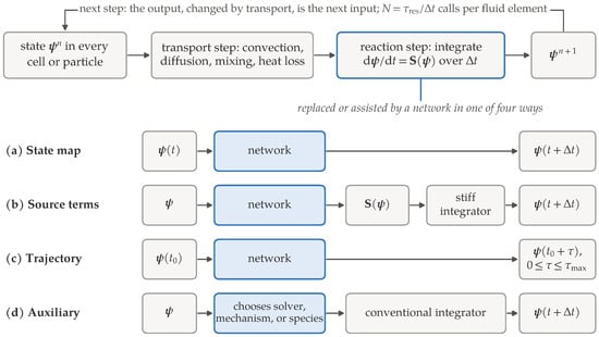
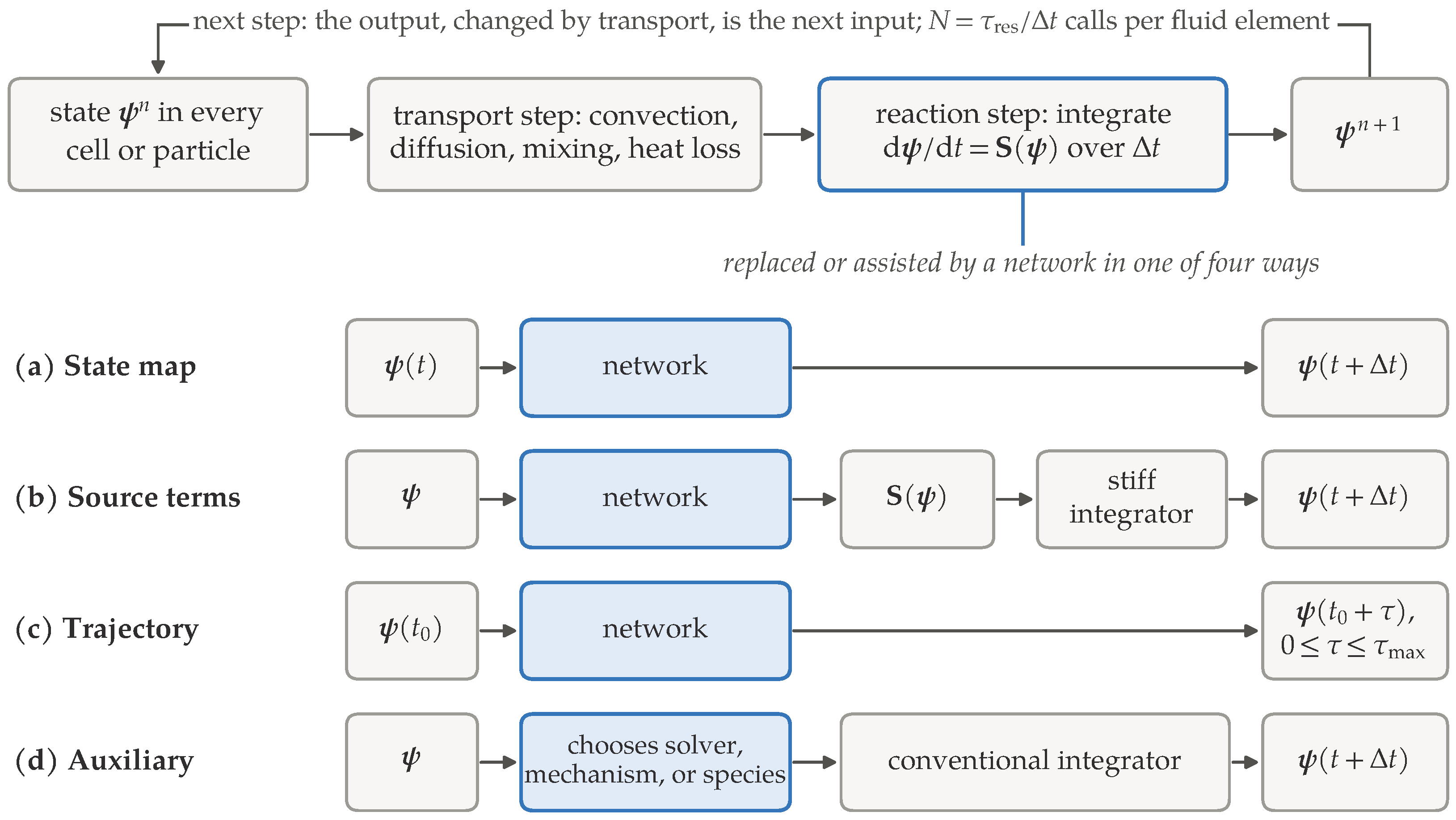
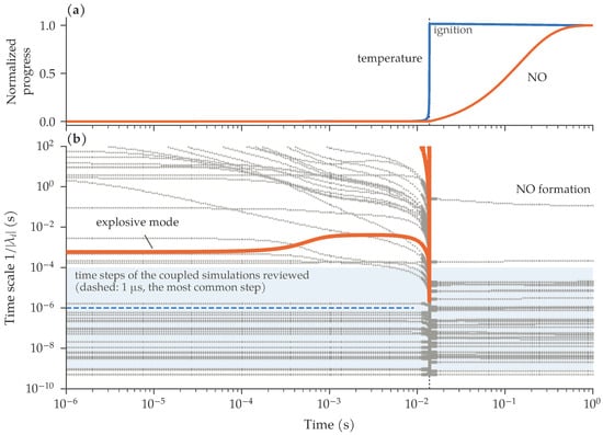
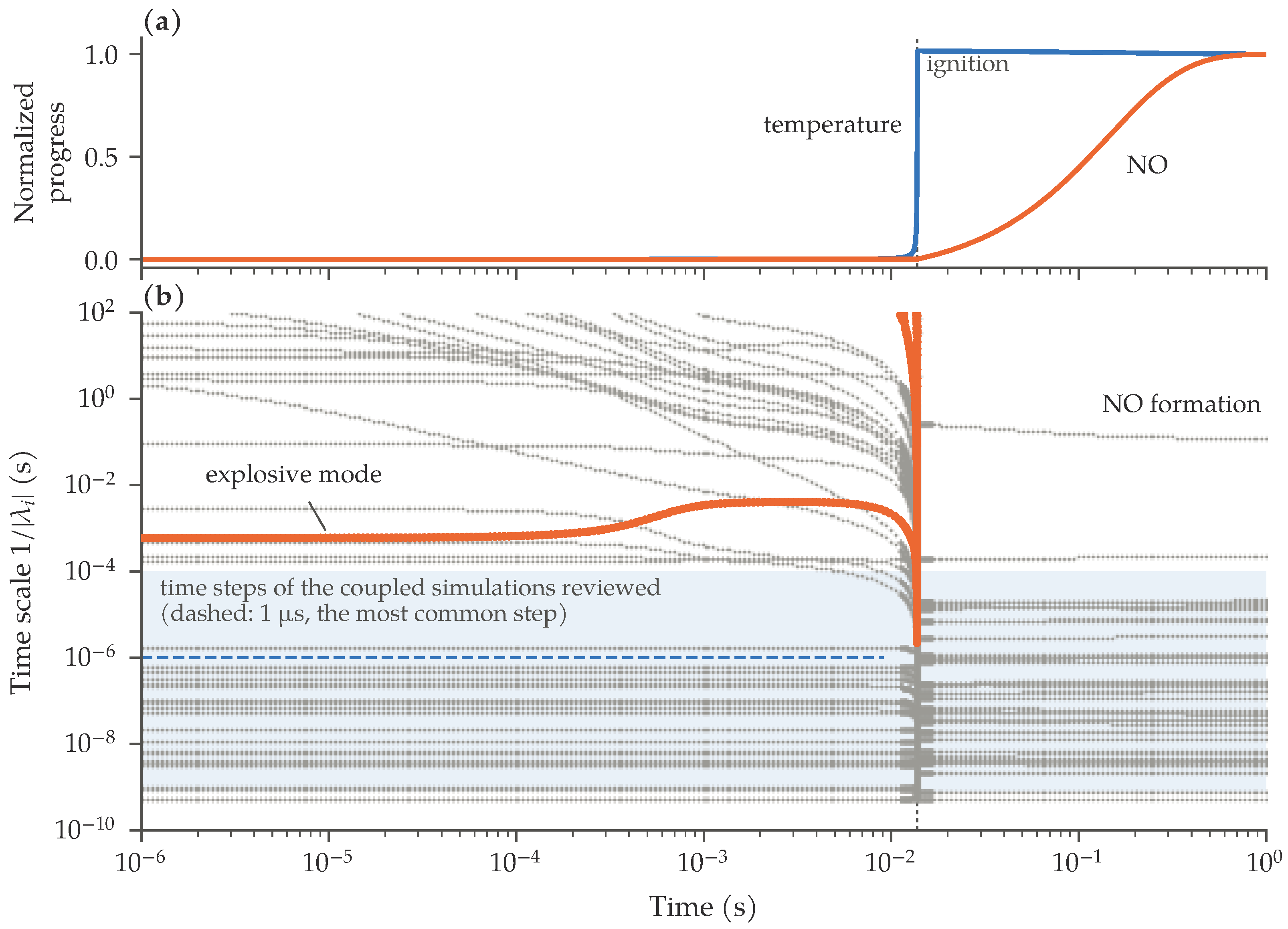
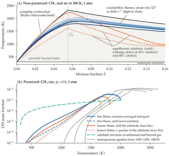
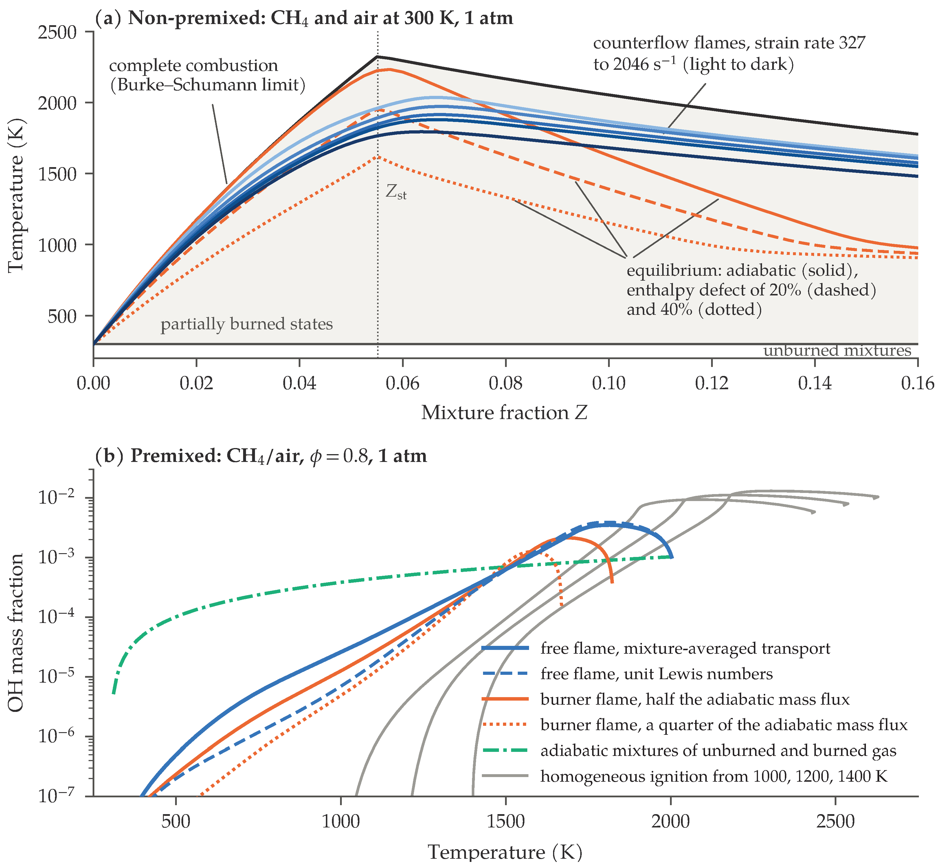
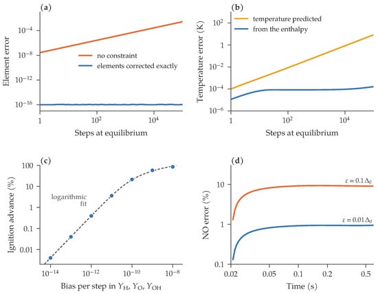
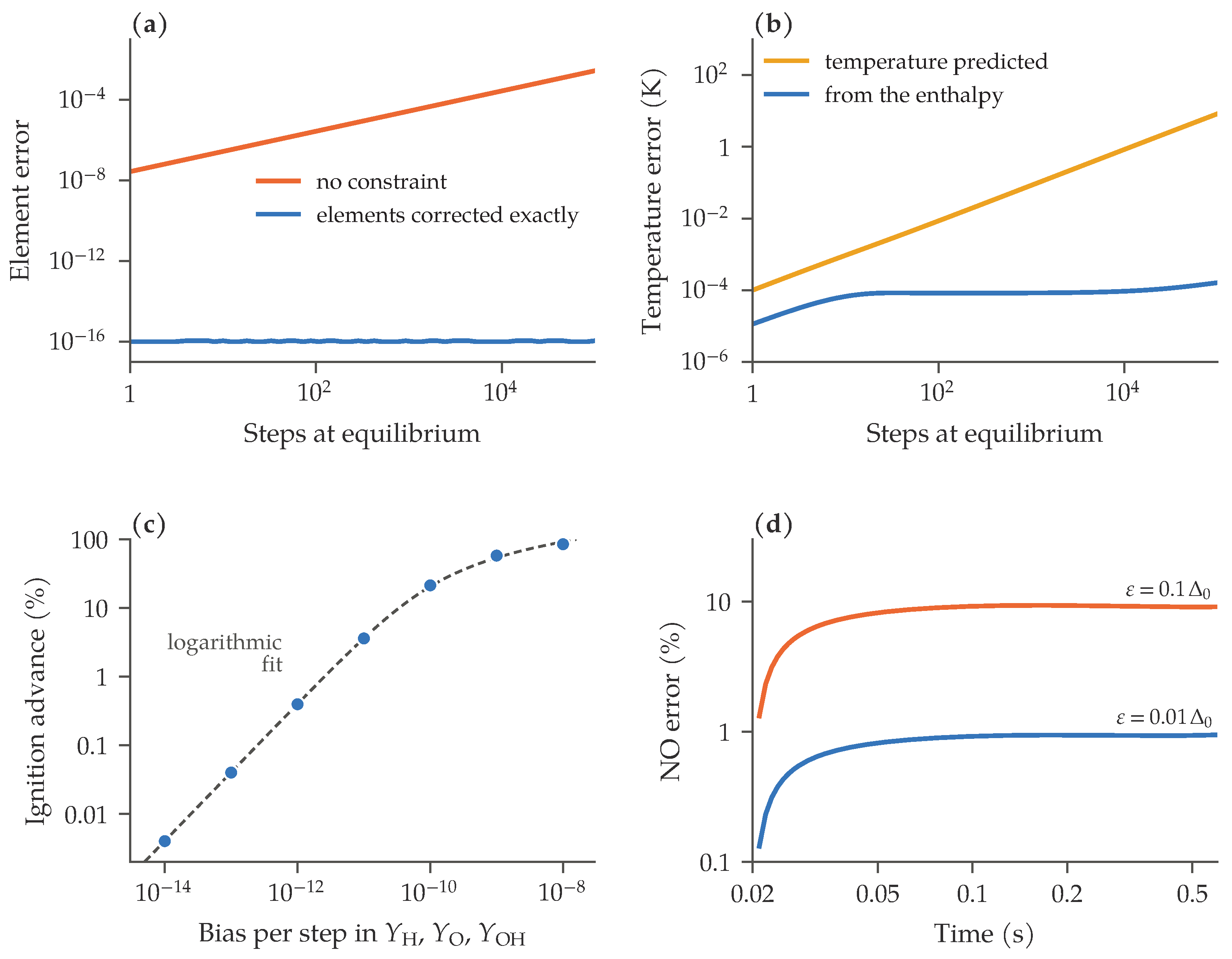
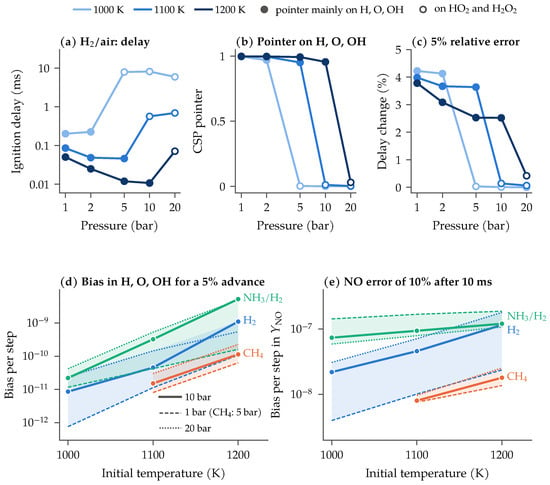
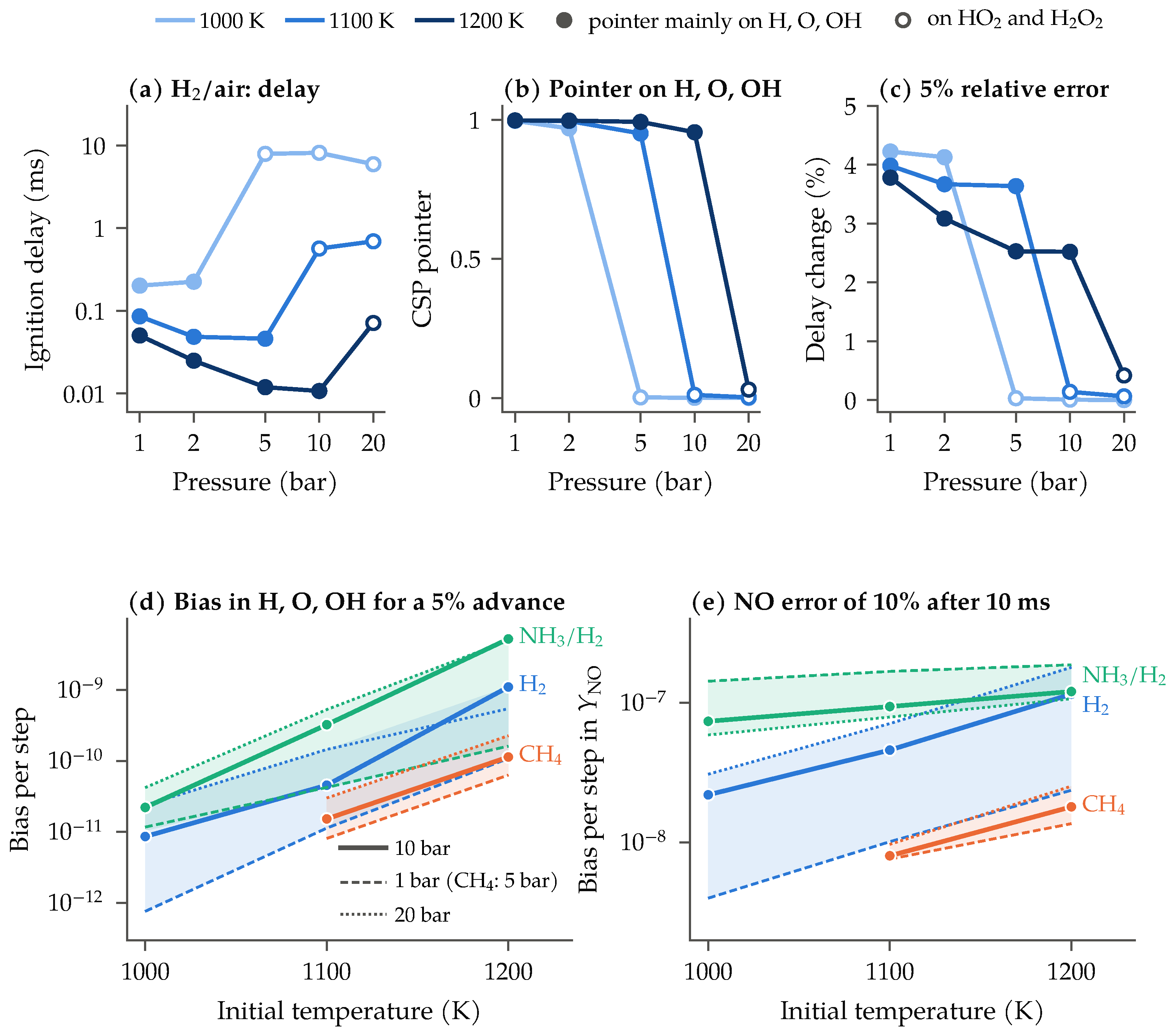
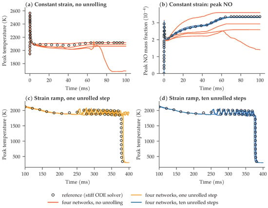
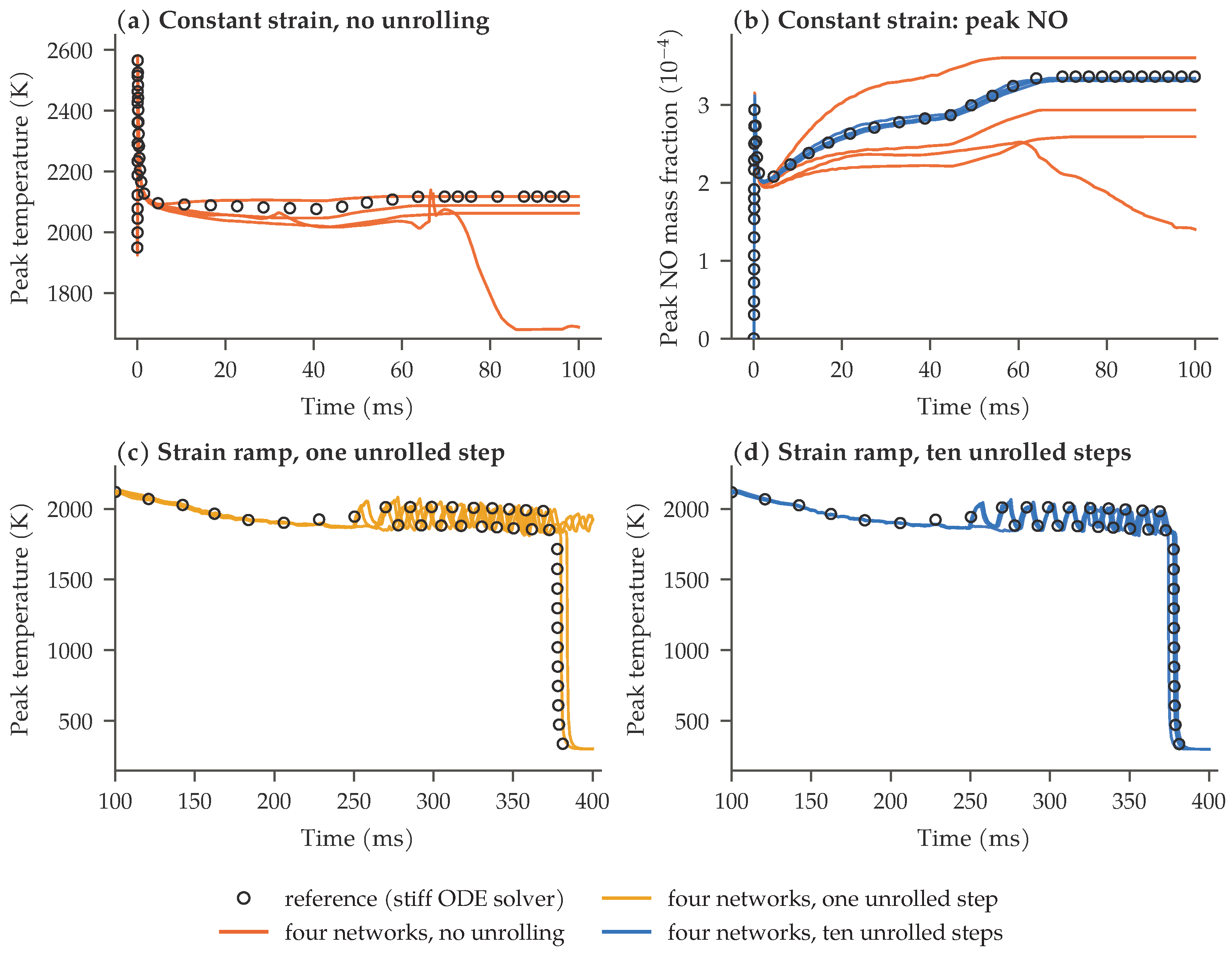
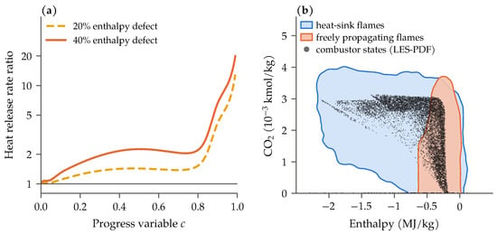
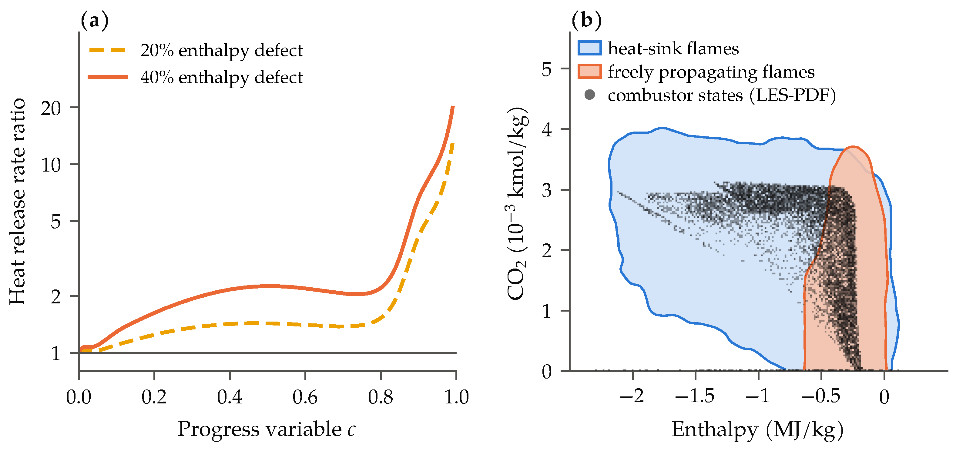
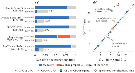
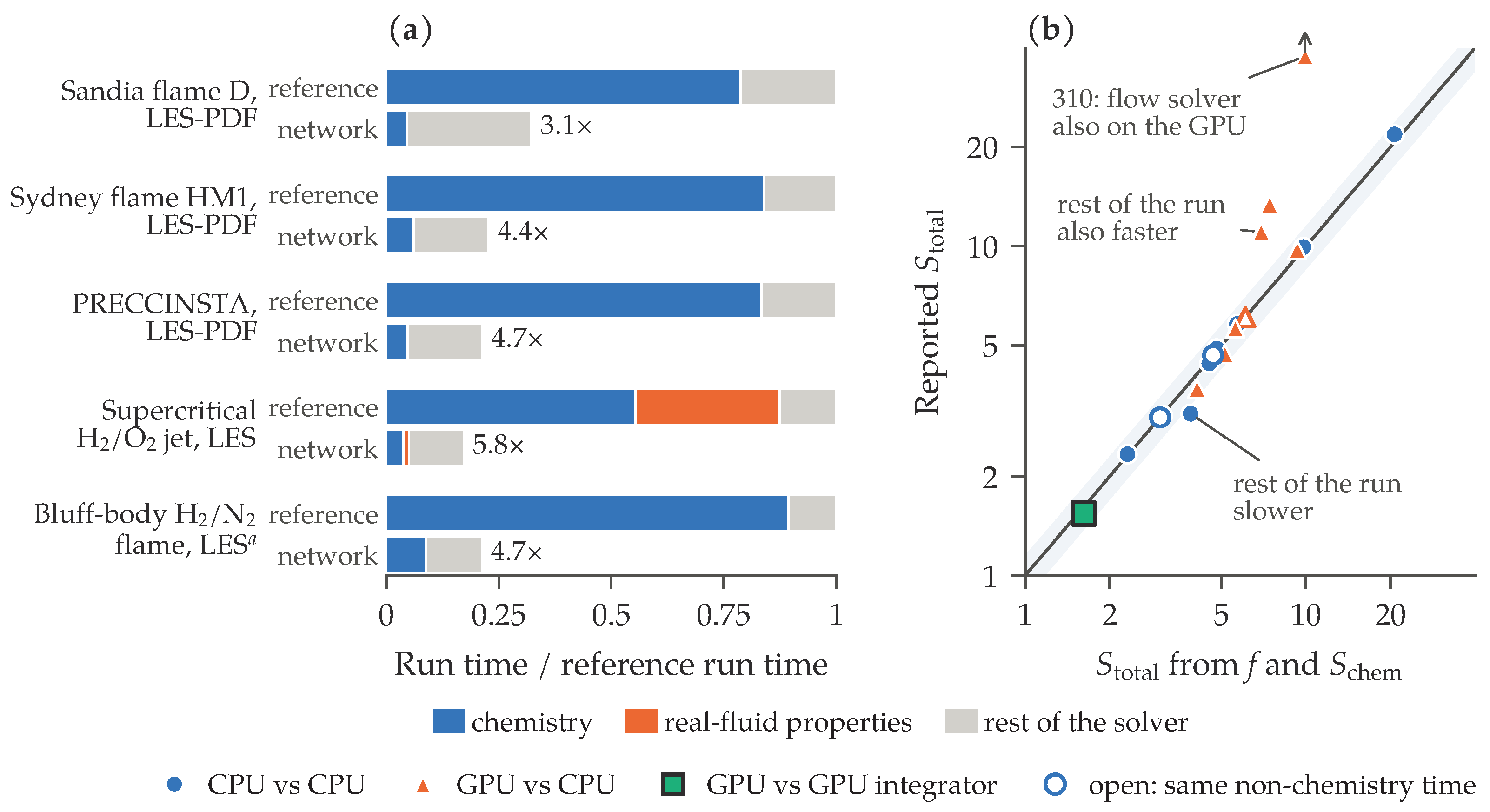

Disclaimer/Publisher’s Note: The statements, opinions and data contained in all publications are solely those of the individual author(s) and contributor(s) and not of MDPI and/or the editor(s). MDPI and/or the editor(s) disclaim responsibility for any injury to people or property resulting from any ideas, methods, instructions or products referred to in the content. |
© 2026 by the authors. Licensee MDPI, Basel, Switzerland. This article is an open access article distributed under the terms and conditions of the Creative Commons Attribution (CC BY) license.