


Abstract
Refrigerated warehouses are among the most energy-intensive food storage facilities, with their thermal performance influenced by local climatic conditions and building envelope characteristics. This study investigates the influence of thermal behavior of a refrigerated warehouse, west wall, under three representative Romanian climatic conditions (Iasi, Cluj-Napoca, and Constanta), using dynamic simulations performed in TRNSYS and a steady-state calculation approach implemented in EES. The TRNSYS simulations were conducted using hourly meteorological data over a complete year (8760 h), while the evaluation focuses on hours 2089–7129 (5041 hourly observations), selected to examine the high cooling demand period. The analysis across the three locations examines the influence of outdoor air temperature and solar radiation on heat transfer through the refrigerated warehouse selected envelope and their influence on the refrigeration load required to maintain the prescribed indoor temperature. Relative humidity is considered separately in the assessment of condensation risk within the wall assembly. For Iasi, the transient thermal behavior of the west-oriented wall is examined in detail through the evolution of its indoor and outdoor surface temperatures and heat flux, together with a comparison between the TRNSYS dynamic simulation and the hourly quasi-steady-state calculation performed in EES. The findings indicate that local climatic conditions influence variations in heat transfer and refrigeration load during the investigated period, as expected, and emphasize the difference between the two approaches. For the wall examined in Iasi, the indoor surface temperature exhibits relatively small variations, whereas the heat flux does not always follow the instantaneous changes in outdoor air temperature. This behavior is consistent with heat storage and release within the multilayer wall assembly, reflecting the transient nature of heat transfer. The EES–TRNSYS comparison for Iasi allows differences between steady-state and dynamic representations of heat transfer to be identified, highlighting the relevance of the wall thermal response when interpreting heat flux variations under the investigated climatic conditions.
1. Introduction
The preservation of perishable food products relies on cold chains capable of limiting biological and chemical degradation processes throughout storage and distribution. Refrigeration therefore plays a direct role in maintaining product quality and extending food shelf life; however, the thermal conditions required along the cold chain are associated with continuous energy consumption. In this context, energy-efficiency measures have become an essential component of sustainable cold-chain management, addressing not only refrigeration systems but also storage facilities, operational strategies, and the integration of renewable energy sources [1]. Refrigerated warehouses play an important role within this framework because they operate for extended periods under large temperature differences between the indoor and outdoor environments. In this context, Meneghetti et al. [2] investigated the integration of renewable energy sources into refrigerated warehouses. Authors emphasized how photovoltaic panels used to fuel refrigerated warehouses can lead to both yearly total cost and energy savings. They have also revealed how different climate conditions affect the economic and environmental performance of such systems. In order to mathematically model energy systems, two main approaches could be considered: steady-state, based on instantaneous response of the system to external factors, and dynamic one respectively, taking into account time response and influence on parameter variation. Transient modeling is an important part of late studies applied to refrigerating systems and has also been extended to other components of the cold chain, including refrigerated transport [3], emphasizing the importance of this approach. The need to represent climatic actions as time-dependent thermal excitations was highlighted by Larsson [4], who examined thermal effects induced by outdoor conditions and solar radiation. Citing Larsson’s work, Manconi et al. [5] used outdoor temperature and solar radiation time series to evaluate the transient thermal response of exposed surfaces.
The energy consumption of refrigerated warehouses is influenced by both the operating conditions imposed on the refrigeration system and the thermal loads entering the refrigerated space. Assessments conducted in commercial cold stores have shown that energy consumption can be reduced through measures targeting space heat loads, equipment operation, control settings, defrost cycles, and other operating parameters [6]. Along the same lines, Evans et al. [7] investigated improvements in the energy performance of cold stores through practical energy-efficiency measures, presenting results from 28 cold store audits across Europe. Their study emphasizes a potential for large energy savings to maximum 72% by optimizing usage of stores, repairing equipment and retrofitting of energy efficient equipment.
From a building perspective, Singh et al. [8] examined the influence of passive strategies associated with the building envelope and climatic conditions on the cooling demand of potato storage facilities. At a more detailed scale, Chourasia and Goswami [9] highlighted the interaction between heat transfer, airflow, and moisture transport in a commercial cold store, with direct effects on temperature distribution and storage conditions.
A recent comparison of experiments, CFD simulations, and refrigeration-load calculation software further indicate that the representation of heat-transfer mechanisms can influence the numerically predicted refrigeration load [10]. Their study emphasizes the importance of relations used to calculate convective and radiation heat transfer, underlying differences of up to 236% in heat load estimates. Their study is very important for rigorously applying empirical correlations in their validity conditions.
The thermal response of a refrigerated warehouse envelope cannot be described solely by a steady-state thermal transmittance (U). The thermal inertia of the wall alters the temporal relationship between the external thermal excitation and the heat flux transmitted towards the interior, even for building components with comparable thermal transmittance values [11]. Heat transfer through multilayer components is governed by the thermophysical properties of the constituent materials and by the boundary conditions applied at the two surfaces, in accordance with classical building-physics formulations and standardized calculation methods, as shown in [12,13]. When moisture transport is also considered, temperature and water-vapor partial-pressure gradients introduce additional coupled processes within the wall structure. The models developed by Künzel [14] and Tariku et al. [15,16], together with general treatments of the hygrothermal behavior of buildings [17], provide the theoretical basis for the transient assessment of coupled heat and moisture transfer. The numerical simulation frame of these processes is addressed in EN 15026 standard [18]. Furthermore, experimental determination of the thermal resistance of building components remains relevant for evaluating the parameters used in numerical models, as revealed in paper [19] by a comparison of different measuring methods of building fabric thermal resistance. The study published in Thermo [20] addressed conductive heat transfer and water vapour diffusion through the multilayer wall of a refrigerated warehouse, examining the thermal and hygrothermal properties of the constituent materials and the functions of the insulation and vapour barrier. Building on this formulation, the present analysis evaluates the transient thermal response of the wall under hourly climatic boundary conditions and relates the resulting refrigeration load to compressor electrical power and energy consumption.
For exterior walls, climatic conditions introduce an additional source of transient variation. Outdoor air temperature, solar radiation, long-wave radiative exchange, and wind-dependent convection jointly contribute to the energy balance at the external surface. The external convective heat-transfer coefficient is particularly sensitive to wind speed and to the correlation adopted in the numerical model, as emphasized in the review by Palyvos [21]. Classical engineering correlations for forced convection over exposed surfaces are also presented in the fundamental work of McAdams [22].
The influence of wall orientation on the transient thermal response of buildings has also been examined by Stanciu et al. [23], who investigated the thermal behavior of a two-story residential building under clear-sky conditions. Their analysis identified the main contributors to building heat losses and examined how the contribution of exterior walls to the thermal load varies with orientation. The study also highlighted the phase shift in the thermal response of the investigated walls. In a related investigation, Stanciu et al. [24] analyzed the influence of heat gains through differently oriented building elements on the indoor thermal conditions of rooms in a public building in Bucharest. Under conditions without mechanical ventilation or air conditioning, the maximum indoor air temperature occurred at approximately 9:00 AM in the room with an east-facing exterior wall, whereas the room with a west-facing exterior wall reached a slightly higher maximum at approximately 4:00 PM. Together, these findings illustrate the combined influence of wall orientation, solar exposure, and thermal inertia on the magnitude and timing of the thermal response, providing additional motivation for investigating transient heat transfer through west-facing walls.
The influence of envelope design on building cooling demand has also been investigated through dynamic thermal simulations. Berger et al. [25] examined external insulation and internal heat gains in office buildings in Vienna, finding that external insulation can slow nocturnal cooling during summer. Dabaieh et al. [26] compared 37 roof configurations for residential buildings in Cairo, assessing how roof geometry, materials and high-albedo surface treatments affect indoor thermal conditions and cooling energy requirements. At the climatic scale, Jylhä et al. [27] used IDA ICE to evaluate residential heating and cooling demand under historical and projected weather conditions in Finland. These investigations provide methodological context for assessing climate-dependent cooling demand, although their applications concern building air conditioning rather than frozen-food storage.
Heat gains through the building envelope ultimately contribute to the load imposed on the refrigeration system and therefore cannot be fully analyzed independently of refrigeration-system performance. Classical refrigeration-system analysis relates evaporating and condensing temperatures to refrigeration capacity, compressor work, and the coefficient of performance [28,29].
System-level studies of supermarket refrigeration systems further show that outdoor temperature and condensing-temperature control can affect electrical energy consumption. Arias and Lundqvist [30], for example, investigated the energy implications of floating condensing-temperature operation under varying outdoor conditions. Cecchinato et al. [31] investigated the energy performance of integrated refrigeration and air-conditioning systems and subsequently extended the analysis to systems using natural refrigerants [32]. Transcritical CO2 configurations with heat recovery were, in turn, investigated by Sawalha [33] and Polzot et al. [34]. Although these studies address refrigeration configurations that differ from those typically encountered in conventional refrigerated warehouses, they highlight the thermodynamic relationship between the thermal load imposed on the system, operating temperatures, and electrical energy consumption.
Energy efficiency, transient heat and moisture transfer through multilayer walls, the influence of climatic conditions, and refrigeration-system performance have been investigated as relevant aspects of refrigerated warehouse operation. However, these research directions are frequently addressed separately. Studies focusing on refrigerated warehouses often examine overall energy consumption or indoor airflow distribution, whereas investigations of the building envelope address transient transfer processes without necessarily tracing the resulting thermal response through to the refrigeration load. Conversely, refrigeration-system studies frequently assume a prescribed cooling load without explicitly resolving its hourly dependence on wall orientation, solar exposure, and local meteorological conditions. This separation limits an integrated assessment of how climatic excitation applied at the external wall surface propagates through the envelope and ultimately affects the energy performance of the refrigerated warehouse.
The present study extends our previous conference paper [35], which investigated the dynamic thermal behavior of a refrigerated warehouse using TRNSYS, with particular attention to the influence of wall orientation on heat transfer through the building envelope. The findings of that investigation provided the basis for selecting the west-facing wall for a more detailed analysis.
Unlike the previous study, the present work focuses on the thermal and hygrothermal behavior of a reference area of 1 m2 of the west-facing wall. The analysis examines the influence of insulation and vapor-barrier thickness on heat transfer and moisture-related performance, supported by a quantitative comparison between the EES and TRNSYS results. Furthermore, the calculated wall heat-transfer load is linked to a two-stage ammonia refrigeration cycle to evaluate the corresponding specific compressor electrical energy consumption. Two analytical relationships describing the exergetic efficiency of the refrigeration cycle are also introduced to assess the influence of operating temperature conditions on compressor performance. These contributions extend the scope of the previous research by connecting the transient thermal response of the building envelope with its hygrothermal characteristics and the associated refrigeration energy requirements.
2. Materials and Methods
2.1. Description of the Studied System
The investigated cold storage facility has a near-square plan to limit the surface-to-volume ratio and the associated transmission heat gains. The layout comprises four chambers (DC1–DC4) separated by insulated internal walls. Chamber DC1 measures 12 m × 12 m × 4 m. Access to the refrigerated spaces is provided through a northern loading dock used for loading and unloading. Wall dimensions and orientations are specified for the heat transfer analysis. The layer thicknesses and thermal conductivities used in the envelope model are listed in Table 1.
Table 1.
Thermophysical properties of the multilayer external wall assembly.
The selected wall configuration consists of a multilayer system comprising exterior and interior plaster layers, expanded concrete masonry, a vapor barrier, and a polystyrene insulation layer.
The initial heat flux peaks decreased progressively as the exclusion period was extended, while the maximum retained heat flux remained unchanged between the 144 h and 168 h thresholds. Based on this comparison, the first 144 h were excluded from the extended evaluation to reduce the influence of initialization transients. The principal analysis of the high cooling demand period, covering hours 2089–7129, was unaffected by this adjustment.
The storage facility thermal behavior was analyzed under the climatic conditions of three representative Romanian cities, namely Iasi, Cluj-Napoca, and Constanta. These locations were selected to represent different climatic sub-regions characterized by distinct outdoor temperature and humidity regimes. Their geographical distribution within Romania is presented in Figure 1. Constanța is located on the Black Sea coast, where the maritime influence results in mild winters and warm summers moderated by sea breezes. Among the three investigated locations, it exhibits the highest average annual outdoor temperature (11.53 °C) together with a high and relatively stable average annual relative humidity (79.13%). In contrast, Iasi experiences the largest annual thermal amplitude, characterized by cold, windy winters and hot summers. The average annual outdoor temperature is 9.45 °C, while the average annual relative humidity reaches 74.98%, with more pronounced seasonal variations than in Constanta. Cluj-Napoca, situated in a hilly basin, records the lowest average annual temperature (8.59 °C) and the highest average annual relative humidity (80.37%). Its climate is characterized by cool summers and long, relatively mild winters, reflecting the moderating influence of the surrounding topography.
Figure 1.
Location of the investigated cities in Romania: Iasi, Cluj-Napoca, Constanta.
Considering the indoor set-point temperature of −20 °C maintained inside the refrigerated chambers, the temperature difference between the indoor and outdoor environments may be as low as 4 °C under winter conditions, when the outdoor temperature reaches −16 °C. In contrast, during summer conditions, outdoor temperatures of up to +35 °C may result in a temperature difference of 55 °C. Furthermore, short-term outdoor temperature fluctuations of up to 10 °C can occur, particularly during the warm season, leading to significant variations in the thermal load imposed on the building envelope.
Climatic differences among the three locations affect both the magnitude and temporal distribution of the thermal loads imposed on the envelope. Under dynamic conditions, the influence of outdoor air temperature on the heat flux transmitted into the refrigerated space also depends on convective and radiative exchanges at the external surface and the ability of the multilayer wall assembly to store and release heat. As a result, variations in the heat flux at the internal wall surface do not necessarily follow instantaneous changes in outdoor air temperature. This behavior is further examined through the transient thermal response of the investigated wall in Iasi. Although outdoor relative humidity is not directly included in the thermal and refrigeration energy calculations, the study also examines moisture-related behaviour through a separate assessment of surface and interstitial condensation risk in the multilayer wall assembly.
To provide a more complete description of the climatic conditions considered in this study, Figure 2 illustrates the hourly variation in outdoor air temperature for Iasi, Cluj, and Constanta over the entire annual simulation period (8760 h). Together with the outdoor relative humidity, Figure 3, these parameters characterize the environmental conditions governing the transient heat and moisture transfer through the refrigerated warehouse envelope.
Figure 2.
Variation in outdoor air temperature (te) for Iasi, Cluj, and Constanta.
Figure 3.
Variation in outdoor relative humidity for the three representative climatic locations: Iasi, Cluj, and Constanta.
Figure 3 shows that the three representative climatic locations exhibit similar annual trends in outdoor relative humidity, while differing in the magnitude and temporal distribution of humidity fluctuations. Iasi presents the most pronounced seasonal variability, characterized by lower humidity values during the warm season and higher values during the colder months. Cluj follows a comparable pattern, although with a slightly more uniform annual distribution. In contrast, Constanta maintains generally higher and more stable relative humidity throughout the year, reflecting the moderating influence of the Black Sea. Although outdoor relative humidity is not directly included in the predictive model, it provides an important climatic descriptor for interpreting the transient thermal and hygrometric response of the refrigerated warehouse envelope under different environmental conditions.
2.2. Mathematical Modelling of Heat Transfer
The mathematical model is used to dig deeper inside heat transfer mechanisms, as detailed in Figure 4, to calculate the temperatures on the outer and inner sides of the outer wall of the cold storage facility and to calculate heat loads the facility is subjected to, firstly under steady-state conditions. The model will be further correlated with the numerical simulations performed in the TRNSYS environment for the transient regime, emphasizing wall thermal inertia and its importance.
Figure 4.
Heat transfer mechanisms through the outer wall of a cold storage facility from the external environment to the cold room.
(i) Description of the physical phenomenon
Let us consider a flat, multi-layer wall, with conductive thermal resistance which separates the external environment (air at temperature te) from the refrigerated space (air at temperature ti).
The outer face of the wall has a temperature tpe induced by heat transfer mechanisms by: convection with outside air (qconv,e) considering a convection coefficient he, absorbed solar radiation (qsol), long-wavelength thermal radiation (qrad) with the surroundings considering a radiative equivalent coefficient hrad and surroundings temperature trad.
These heat streams converge and pass through the wall through conduction (qcond) and turn inside into a single convective flow to the cold air for which a convection coefficient hi is considered. Accordingly, on the inner face, the wall temperature tpi is further determined.
(ii) Equations and solving algorithm
Heat flux densities [W∙m−2] are computed according to Newton, Fourier and Stepfan-Boltzmann heat transfer laws:
- -
- thermal conduction through the wall:
- -
- convection on the outer face of the wall:
qconv,e = he(te − tpe)
- -
- thermal radiation of long wavelength (infrared) to the outside:
- -
- absorbed solar radiation:
qsol = αs∙Is
- -
- indoor convection:
qconv,i = hi(tpi − ti)
The heat transfer is considered to take place in a steady-state regime:
q = qconv,e + qrad + qsol = qcond = qconv,i
Energy balance equations on the outer and inner wall surfaces lead to determination of tpi and tpe function on known data (ambient parameters and imposed interior air temperature). Consequently, the following equations might be written:
- -
- energy balance on the outer wall surface:
- -
- energy balance on the inner wall surface:
Unknown values of wall surface temperatures tpi and tpe are determined by solving Equations (7) and (8) together.
A further analytical development might be performed. Solving Equation (8) one obtains:
After replacing tpi from Equation (9) in (8), one obtains
in which
represents the overall coefficient of heat transfer through wall conduction and convection at the interface between the inner wall and the air in the refrigerated room.
It follows that:
q = Upe,i(tpe − ti),
Taking into account Equations (4), (7) and (12), Equation (6) becomes:
This equation is numerically solved for the temperature of the outer face of the wall, tpe. Once the problem is solved for tpe, substituting its value into Equation (9) gives the temperature of the inner surface of the wall tpi.
The density heat load transferred through the wall from the external environment to the inside of the cold room is now determined by Equation (6). This is an important variable of the problem for further determining the system response in terms of electric energy consumption to any change in environmental parameters or materials.
2.3. Sol-Air Outside Temperature (Tsa)
The sol (solar)–air temperature concept combines the effects of convection, solar radiation and thermal radiation in a single parameter.
The thermal balance on the outer surface of the wall includes convection with the outside air (Equation (2)), thermal radiation with the envelope of the external environment (sky + buildings + ground) (Equation (3)) and absorption of solar radiation (Equation (4)).
If the three heat fluxes are summed up, the result is:
q = he (Te − Tpe) + hrad (Trad − Tpe) + αs∙Is
Convection and radiation external heat flux is assimilated with a single convective effect:
where the global external heat transfer coefficient is:
q = ho (Tsa − Tpe)
ho = he + hrad,
Developing Equation (14) it follows that:
q = he∙Te + hrad∙Trad + αs∙Is − (he + hrad)Tpe,
Taking into account the notation from Equation (16), Equation (17) becomes:
q = he∙Te + hrad∙Trad + αs∙Is − hoTpe,
Identifying Equations (15) with (18) one obtains:
and finally
hoTsa = he∙Te + hrad∙Trad + αs∙Is,
Tsa = (he∙Te + hrad∙Trad + αs∙Is)/(he + hrad),
Sol-air temperature Tsa is a fictitious temperature that the air would have and a function of which the sum of all types of heat transfer from the outside is assimilated to a convective heat transfer from the air to the outer face of the wall.
In a similar way, Trad is the temperature of a fictitious black body that would change the sum of the radiant heats from the environment (sky + surrounding objects + ground) with the outer wall surface.
2.4. Refrigeration System Electric Power Consumption
In steady-state operation of maintaining a constant temperature of the refrigerated products, the refrigeration system evacuates the heat load transferred from the outside through the walls of the refrigerated room.
Due to the large temperature difference between condensation and vaporization ∆T = Tc − Tv (50 − 80 K), a two-stage refrigeration system is chosen: a high-performance cycle with two throttling valves, flash intermediate cooling followed by a liquid separator. The diagram of the refrigeration plant and the representation of the cycle processes in T-s coordinates are shown in Figure 5.
Figure 5.
Two-stage refrigeration system with full intermediate cooling and two throttling processes. (a) System diagram; (b) cycle representation in T-s diagram.
The refrigerant used is Ammonia (NH3), a natural refrigerant with excellent thermodynamic properties given that the cold store is located outside a dense urban agglomeration.
The temperature kept constant in the warehouse is ti = −20 °C, as previously defined.
Due to the use of secondary fluid for heat transfer, a temperature difference ∆Tv = 10 K is chosen in the evaporator (5 K from the inside air-cooling space to the secondary fluid and another 5 K from the fluid to the vaporizing NH3). Consequently, the evaporation temperature is determined:
tv = ti − 10 = −30 °C
In the condenser, a temperature difference of ∆Tc = 5 K is considered, so that the condensation temperature of the refrigerant is:
tc = te + ∆Tc
The focus is now to calculate the electric energy consumption of the refrigeration system according to the temperature lift ∆T = Tc − Tv, where Tv = constant and Tc(Te) follows environmental temperature fluctuations.
The calculation is presented for evacuating the unit heat load computed by Equation (6).
The exergetic (second-law) efficiency of the refrigeration cycle is:
in which
is the specific cooling power, [kg/s] is the refrigerant mass flow rate passing the evaporator, w [J/kg] is the compressor specific shaft work related to density heat load transfer (for 1 m2 wall), while indices LPcp and HPcp refer to low pressure (first stage) compressor and high pressure (second stage) compressor, respectively.
The term μ is used for the mass flow rate ratio between second and first compressor stages.
Equation (23) becomes:
In Equation (25) the ratio represents the coefficient of performance of a Carnot cycle refrigeration system that operates extracting heat from the temperature Tv and transferring it to the ambient temperature Te.
It follows from Relation (25) that
and finally
Equation (25) can be graphically represented emphasizing the exergetic efficiency dependence on the temperature difference ηex(∆T = Te − Tv). Thus, Figure 6 is plotted, in which the red solid line shows the exergetic efficiency calculated for the standard cycle, while the blue dashed line represents its second-order polynomial fit. Isentropic efficiency of 0.8 was considered for both compressor stages.
Figure 6.
The exergetic efficiency of the standard cycle dependence on the temperature lift between the vaporization and the ambient—red curve; the blue curve is the polyfit.
This allows determining the analytical function of the graphical representation ηex(∆T = Te − Tv) as:
and will be used in the calculation of the electric power consumed by refrigerating system compressor, corresponding to each outside temperature Te.
ηex = 0.584584132 + 0.0023231269∙∆T − 0.0000264797159∙∆T2
2.5. TRNSYS Numerical Simulation
The dynamic simulations were performed using TRNSYS Type 56, which provides the convective and radiative heat transfer rates at the internal surface of each exterior wall. The schematic of the studied system built in TRNSYS environment is presented in Figure 7. The transient thermal simulations were performed using TRNSYS 17 (version 17.01.0025), with Simulation Studio version 5.3.0.0.
Figure 7.
Computational workflow of the proposed TRNSYS model.
The refrigerated storage facility was represented using Type 56, which performs the dynamic thermal simulation of the building envelope and indoor zones. The meteorological data used in the dynamic TRNSYS simulations were obtained from Meteonorm weather files in TM2 format, corresponding to the Typical Meteorological Year (TMY2) format. Hourly meteorological data, with a temporal resolution of 1 h, were considered for three Romanian climatic locations: Iasi (47.17° N, 27.60° E; altitude 104 m; RO-Iasi-150900.tm2), Cluj-Napoca (46.78° N, 23.57° E; altitude 410 m; RO-Cluj-Napoka-151200.tm2), and Constanta (44.22° N, 28.63° E; altitude 13 m; RO-Constanta-154800.tm2). These meteorological files provided the climatic boundary conditions required for the transient thermal analysis of the refrigerated warehouse envelope.
Hourly weather conditions were introduced through Type 15, providing ambient temperature, relative humidity, wind speed and solar radiation data. Solar radiation incident on each wall orientation was determined using Type 16, while the sky temperature was evaluated through an auxiliary model based on the meteorological inputs. Additional psychrometric calculations and model parameters were incorporated to determine the external boundary conditions required for the transient heat-transfer analysis. The individual components were interconnected to ensure the continuous transfer of climatic and thermal information throughout the simulation. Consequently, the weather data directly influenced the conductive, convective and radiative heat transfer through the building envelope, allowing the refrigeration load to be evaluated under realistic operating conditions. The developed simulation framework was specifically designed to quantify the influence of climatic conditions and wall orientation on the refrigeration performance of the cold storage facility.
The heat gains through the building envelope were obtained from convective heat transfer at the internal wall surface and radiative heat transfer at the internal wall surface. This enables the direct evaluation of the total heat gains entering the refrigerated space while simultaneously accounting for both convective and radiative heat transfer mechanisms. The dynamic simulations were performed using TRNSYS 17 and the Type 56 multizone building model, with a simulation time step and wall transfer-function time base of 1 h. The refrigerated warehouse was represented by four thermal zones (ZONE_A1–ZONE_A4), corresponding to the four refrigerated chambers, while the loading dock was not modeled as a separate thermal zone. The indoor temperature was maintained at −20 °C using the ideal cooling function of Type 56. The simulations covered 8760 h, with the detailed analysis restricted to hours 2089–7129 (5041 hourly observations). The investigated west-facing wall of chamber DC1 corresponds to surface S4 (48 m2), with heat-transfer results normalized to 1 m2.
The model included separate constructions for the external and internal walls, roof slab, and floor. Reference temperatures of +20 °C above the roof slab and +1 °C for the ground were specified. Meteorological data from Meteonorm (TMY2 format) were processed using Type 109, while Type 33e provided psychrometric properties and Type 69b calculated the effective sky temperature supplied to Type 56 through TSKY. The effective ground radiative temperature, introduced through TSGRD, was assumed equal to the outdoor air temperature. For the vertical west-facing wall, the sky and ground view factors were both 0.50, with a solar absorptance of 0.40 and a long-wave emissivity of 0.90. No separate Type 16 component was required.
The analysis was designed to isolate heat transfer through the investigated wall rather than determine the total refrigeration load of the warehouse. Accordingly, infiltration, ventilation, and internal heat gains from occupants, lighting, equipment, and stored products were intentionally excluded from the specific refrigeration-load calculation. The thermal contribution of surface S4 was determined from the Type 56 outputs as q_S4 = (QCOMI_S4 − QABSI_S4)/(3.6 × 48), where both outputs are expressed in kJ/h and q_S4 in W/m2. QCOMI includes convective and long-wave radiative exchanges at the internal surface, while QABSI accounts for absorbed radiative gains. The corresponding surface temperatures and external heat-exchange quantities were also extracted from Type 56. The refrigeration electricity demand associated with this wall contribution was subsequently calculated using a separate two-stage vapor-compression cycle, rather than interpreted as the total electricity consumption of the warehouse.
2.6. Recommendations Regarding Convection Coefficients and Insulation and Vapor Barrier Thicknesses
In the mathematical model, the internal convective heat transfer coefficient, hi, was fixed at 8 W·m−2·K−1, while the external convective heat transfer coefficient, he, was calculated using a wind-speed-dependent correlation.
Convective heat transfer at a wall surface can be described by Newton’s law of cooling, which relates the convective heat flux to the temperature difference between the surrounding air and the surface in contact with it:
where qconv,e is the convective heat flux at the external wall surface, expressed in W/m2, te is the outdoor air temperature, tpe is the external wall surface temperature, and he is the external convective heat transfer coefficient, expressed in W/(m2·K). In this formulation, the temperature difference te − tpe provides the driving force for convective heat transfer, he, whereas characterizes the intensity of heat exchange between the moving outdoor air and the wall surface.
qconv,e = he (te − tpe)
Unlike the thermal conductivity of a material, the convective heat transfer, he coefficient is not an intrinsic property of the wall. Its value depends on the flow conditions within the air boundary layer adjacent to the surface and is influenced by wind speed, surface roughness and geometry, as well as airflow direction. The review conducted by Palyvos shows that numerous correlations have been proposed for estimating the external convective heat transfer coefficient, reflecting differences in the experimental conditions and the characteristics of the surfaces considered.
For the refrigerated warehouse considered, the internal and external wall surfaces are exposed to different thermal boundary conditions. On the indoor side, the air temperature is controlled by the refrigeration system. At the external surface, atmospheric conditions vary throughout the year; therefore, assuming a constant convective heat transfer coefficient he would neglect the influence of wind-speed variations on the external thermal boundary condition. Accordingly, he was evaluated at each hourly time step using the wind speed provided by the meteorological data.
The relevance of this variation is also reflected in the thermal resistance of the wall. The external convective thermal resistance is represented by the term , which contributes to the total thermal resistance together with the conductive resistances of the individual wall layers and the internal convective resistance. Consequently, variations affect both the external surface temperature and the temperature distribution across the multilayer wall. This relationship is particularly relevant for refrigerated warehouse walls, where the temperature gradient between the outdoor environment and the refrigerated space persists for extended periods.
At low wind speeds, convective heat transfer does not vanish as the air velocity approaches zero. In this range, linear correlations commonly express the external convective heat transfer coefficient as the sum of a velocity-independent term and a term proportional to wind speed. Larsson [4], citing the CEB (Comite Euro-International du Beton) recommendations for walls and slabs, reports this type of relationship for wind speeds up to 5 m/s.
This supports the use of a linear formulation in the low wind-speed range. Similar correlations are also reported by Palyvos [21] for exposed plane surfaces with different surface roughness characteristics.
where v is the wind speed, expressed in m/s. The constant term maintains a finite convective heat transfer coefficient under low-wind conditions, while the velocity-dependent term accounts for the progressive increase in convective heat transfer as the wind speed increases. Thus, for v = 0 m/s, he = 5.6 Wm−2 K−1, whereas at v = 5 m/s, he reaches approximately 25.35 Wm−2 K−1.
he = 5.6 + 3.95 v for v ≤ 5 m/s,
As wind speed increases, forced airflow exerts a progressively stronger influence on the boundary layer adjacent to the wall surface. In this range, power-law correlations are commonly reported in the literature. The CEB formulation presented by Larsson [4] also distinguishes wind speeds above 5 m/s from the low-velocity range, supporting the use of two separate calculation regimes. In the comparative review by Palyvos [21], the correlation he = 7.6 v0.78 is reported for rough surfaces at higher wind speeds, and the same form is used by Manconi et al. [5]. Accordingly, for v > 5 m/s, the following correlation was adopted:
he = 7.6 v0.78 for v > 5 m/s,
The exponent 0.78 accounts for the nonlinear dependence of the convective heat transfer coefficient on wind speed in a regime where forced convection becomes dominant. At v = 5 m/s, this correlation yields approximately 26.7 Wm−2 K−1, which is close to the value of 25.35 Wm−2 K−1 obtained from the linear correlation.
The threshold of 5 m/s was not introduced arbitrarily. The CEB formulation reported by Larsson [4], the correlations reviewed by Palyvos [21], and the formulation subsequently used by Manconi et al. [5] distinguish between the low wind-speed range and the range in which forced convection becomes more pronounced. Differences among the numerical coefficients reported in these sources reflect the empirical nature of the correlations and the specific conditions under which they were developed. Accordingly, the correlations adopted in the present model are used as an engineering representation of the external convective boundary condition for the vertical walls considered, rather than as universal relationships independent of surface geometry and roughness.
In the hourly calculation, the wind speed is first used to determine the value of by selecting the correlation corresponding to the appropriate velocity range. The resulting value is then introduced into Newton’s law of cooling to calculate the external convective heat flux.
This approach explicitly incorporates the hourly variability of wind speed into the external thermal boundary condition. Variations affect both the convective heat exchange and the external surface temperature, with the resulting thermal response subsequently propagating through the wall by conduction. For the investigated configuration, this formulation provides a more representative description of variable outdoor conditions than the use of a single constant external convective heat transfer coefficient.
A significant fraction of the refrigeration load in cold storage facilities originates from heat transfer through the building envelope. Increasing the insulation thickness reduces the conductive heat gains and improves the thermal performance of the refrigerated space. However, beyond a certain value, additional insulation becomes economically unjustified because the corresponding reduction in heat gains becomes progressively smaller. In what follows, important observations are made for choosing the optimum thickness for the insulation layer, but also for the vapor barrier. In this regard, Figure 8 illustrates the temperature and vapour-pressure profiles across the multilayer wall, together with the directions of heat and water-vapour transfer.
Figure 8.
Schematic representation of coupled heat and moisture transfer through the multilayer external wall assembly (reproduced from Constantin et al. [20] under the terms of the CC BY 4.0 license https://creativecommons.org/licenses/by/4.0/). The vapor barrier was incorporated into the wall assembly in order to limit water-vapor diffusion from the ambient environment toward the refrigerated space and to reduce the risk of moisture accumulation within the insulation layer. The use of vapor barriers in refrigerated buildings is widely recommended because moisture migration may deteriorate the thermal performance of insulation materials and promote condensation-related phenomena [20].
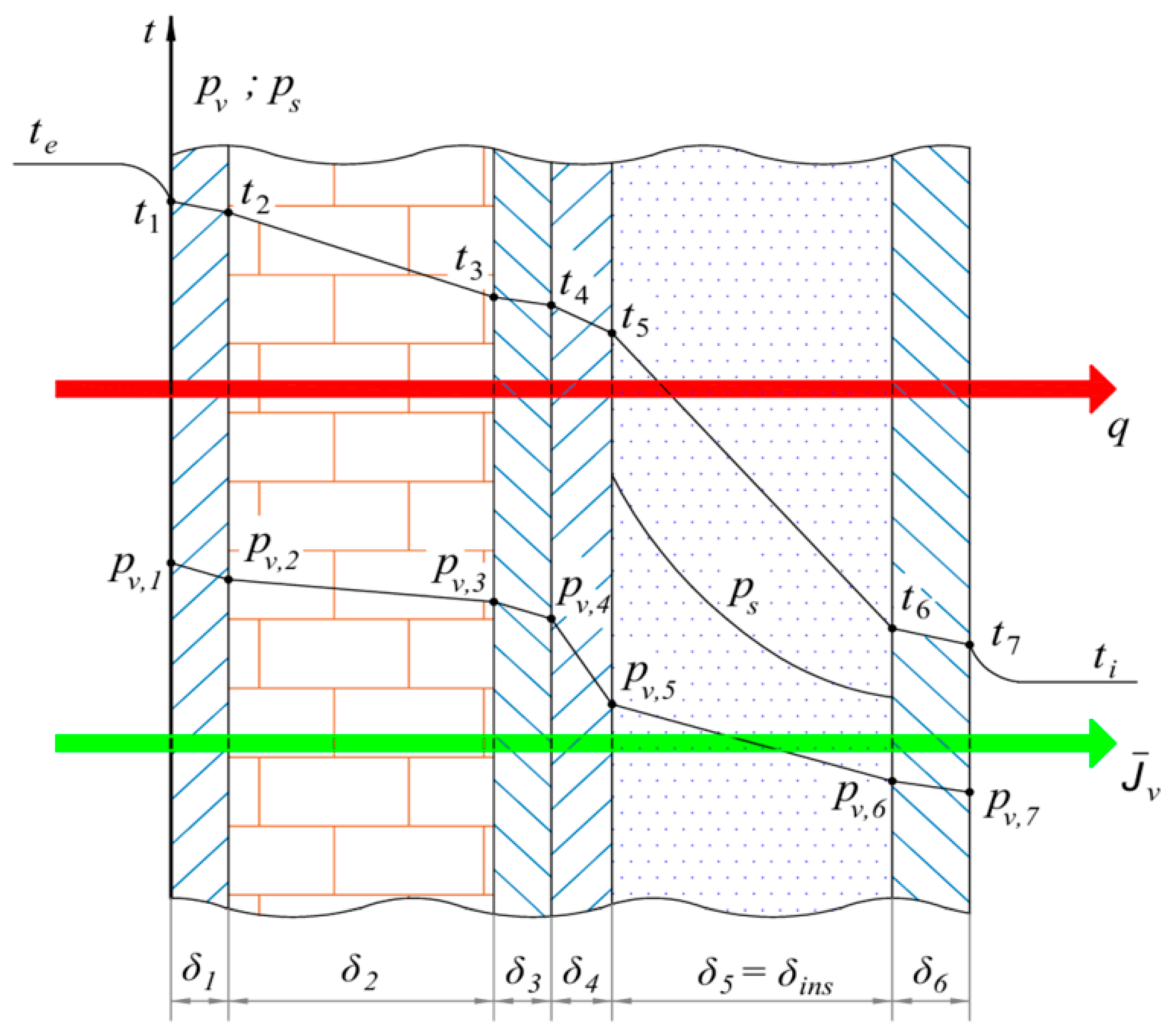
Moisture-related problems in refrigerated facilities may occur in the form of surface or interstitial condensation. Surface condensation develops when the interior wall surface temperature falls below the indoor air dew-point temperature, whereas interstitial condensation occurs when water vapor diffuses into the wall assembly and reaches saturation within its layers. Because interstitial moisture accumulation may progressively reduce the thermal performance of the insulation and accelerate material degradation, the present study focused primarily on this phenomenon. Surface condensation was also verified through the surface safety indicators, confirming the absence of condensation on the internal wall surface throughout the simulation period.
To prevent both moisture mechanisms, the wall configuration was evaluated using complementary surface and interstitial condensation indicators.
The selection of the wall configuration was performed using two complementary criteria. The first criterion was hygrothermal and aimed to identify combinations of insulation and vapor barrier thickness that prevent condensation throughout the entire simulation period. The second criterion considered the thermal performance of the wall through the average overall heat transfer coefficient, allowing the influence of additional material thickness on heat transfer to be evaluated.
The analysis was carried out in two successive stages. First, the influence of the insulation thickness was investigated while maintaining a constant vapor barrier thickness. Subsequently, the insulation thickness selected from the first stage was kept constant, and the vapor barrier thickness was varied in order to determine the minimum thickness capable of eliminating the risk of interstitial condensation over the entire year.
2.6.1. Influence of Insulation Thickness
The influence of insulation thickness was investigated by varying the thermal insulation layer from 8 to 20 cm while maintaining a constant vapor barrier thickness of 24 mm. The assessment was based on two complementary criteria: the hygrothermal response, evaluated using the minimum hygrothermal margin (MM), defined as the difference between the local saturation vapour pressure and the water-vapour partial pressure (MM = p_sat − p_v). Positive MM values indicate that the vapour pressure remains below saturation, whereas negative values indicate conditions associated with interstitial condensation. Table 2 presents the minimum hygrothermal margins obtained for the three investigated climatic locations over the insulation thickness range of 0.08–0.20 m.
Table 2.
Minimum hygrothermal margin as a function of insulation thickness for the three investigated climates.
The minimum hygrothermal margin, MM, remained positive for all three climatic locations throughout the investigated insulation range, indicating that the model predicted no interstitial condensation under the assessed conditions. Increasing the insulation thickness from 0.08 to 0.20 m reduced MM from 38.39 to 23.38 Pa for Iasi, from 35.05 to 20.29 Pa for Cluj, and from 35.05 to 14.09 Pa for Constanta. Thus, although the margin decreased with increasing thickness, the condensation-avoidance criterion remained satisfied across the investigated range.
At an insulation thickness of 0.14 m, MM was 31.77 Pa for Iasi, 31.23 Pa for Cluj, and 28.26 Pa for Constanta. This thickness was retained as the reference configuration for the subsequent analyses; the positive margins confirm its admissibility according to the adopted hygrothermal criterion.
2.6.2. Influence of Vapor Barrier (VB) Thickness
After selecting the insulation thickness, the influence of the vapor barrier thickness was investigated while maintaining a constant insulation thickness of 0.14 m. The vapor barrier thickness was varied to determine the minimum value capable of preventing interstitial condensation throughout the entire simulation period. The resulting minimum hygrothermal margins for the three climatic locations are summarized in Table 3.
Table 3.
Minimum hygrothermal margin as a function of vapor barrier thickness for the three investigated climates.
The tabulated values represent the minimum pressure difference between the local saturation pressure and the water-vapour partial pressure over the simulation. A positive value denotes the available hygrothermal reserve before saturation is reached. A negative value quantifies the extent to which the vapour pressure exceeds the local saturation pressure; under this condition, the excess water vapour can no longer remain in the gaseous state and interstitial condensation occurs.
The influence of vapor barrier thickness differed among the investigated climates. For Iasi and Cluj, the minimum hygrothermal margin increased from negative to positive values as the vapor barrier thickness increased, indicating the gradual elimination of interstitial condensation risk. In Constanta, the same trend was observed, although lower safety margins were obtained for intermediate thicknesses due to the combined effect of higher outdoor temperature and humidity. For the insulation thickness of 0.14 m, the critical vapour barrier thickness is 16 mm. Increasing the vapour barrier thickness beyond this value increases the calculated hygrothermal safety margin.
2.6.3. Recommended Final Configuration
The combined assessment of insulation and vapor-barrier thickness was used to define the wall configuration adopted in the subsequent analyses. An insulation thickness of 140 mm was retained as the reference value based on the thermal and hygrothermal assessment presented above. For the vapor barrier, a thickness of 16 mm was sufficient to prevent water vapor condensation, as indicated by the positive minimum hygrothermal margins obtained in all three climatic locations over the selected 5041 hourly observations (simulation hours 2089–7129). Increasing the vapor-barrier thickness to 24 mm resulted in MM values of 31.77 Pa for Iasi, 31.23 Pa for Cluj, and 28.26 Pa for Constanta. These values coincide with the minimum hygrothermal margins obtained for the 140 mm insulation case, providing a common reference point between the two parametric analyses. Accordingly, a configuration comprising 140 mm of thermal insulation and a 24 mm vapor barrier was retained for the subsequent thermal and energy analyses.
With the wall configuration fixed, the following analysis examines the climatic boundary conditions imposed on the model, focusing on the variations in outdoor air temperature and relative humidity across the three locations.
The primary scope of this paper is not to conduct a comprehensive transient hygrothermal analysis of the building envelope. Rather, the hygrothermal assessment was employed strictly as a preliminary sizing tool to justify the selected dimensions for the wall assembly—specifically, the insulation and vapor barrier (VB) thicknesses—in order to ensure that interstitial condensation is prevented under the investigated conditions.
3. Results
The diurnal evolution of the external and internal surface temperatures was examined for the west-facing wall of cold room DC1 by comparing EES predictions with the corresponding TRNSYS results for sample days in spring, summer, and autumn. These days illustrate the model responses under different climatic conditions without implying seasonal representativeness. The comparison was conducted on a unit-area basis of 1 m2, using the same prescribed boundary conditions for both models. It assesses how closely the quasi-steady EES formulation reproduces the surface temperature levels and temporal variations predicted by the dynamic TRNSYS model. Table 4 lists the input parameters used in both approaches and summarises their heat transfer modelling assumptions.
Table 4.
Comparison of input parameters and heat transfer modelling assumptions in EES and TRNSYS.
The following figures compare the exterior wall surface temperature, t_pe, predicted by EES and TRNSYS for the west-facing wall in Iasi during representative spring, summer and autumn periods.
The comparison in Figure 9 uses three sample days, one each in spring, summer, and autumn, to illustrate differences in the diurnal evolution of the external surface temperature predicted by EES and TRNSYS. These days were selected for graphical illustration rather than according to a formal criterion of seasonal representativeness. The statistical assessment covers all 5041 consecutive hourly observations from hour 2089 to hour 7129, rather than only the three days displayed.
Figure 9.
Comparison of the external surface temperature, t_pe, of the west-facing wall of cold room DC1 in Iasi, calculated using TRNSYS and EES for sample days in (a) spring, (b) summer, and (c) autumn.
EES reproduces the overall evolution of the external surface temperature, t_pe, predicted by TRNSYS, including the successive heating and cooling periods of the wall. Differences arise in the magnitude and timing of the temperature variations. These local differences coexist with a negative mean bias over the analysed seasonal intervals: MBE is −2.090 °C in spring, −2.735 °C in summer, and −1.900 °C in autumn. The discrepancies therefore include both a tendency towards lower EES predictions and variations associated with changing boundary conditions.
During the sample spring day (Figure 9a), both models predict an increase in external surface temperature from negative values to approximately 11–12 °C, followed by cooling. Immediately afternoon, the increasing solar contribution to the west-facing wall provides a useful interval for examining the different model responses. The quasi-steady EES formulation responds directly to the boundary conditions imposed at each time step, whereas TRNSYS also accounts for heat storage and release within the wall. As the external thermal forcing subsequently decreases, stored heat can sustain the surface temperature predicted by the dynamic model, while this storage effect is absent from EES. The spring RMSE of 2.706 °C and MAE of 2.141 °C quantify the discrepancies over the full seasonal interval.
The sample summer day (Figure 9b) exhibits the highest surface temperatures among the three days shown, reaching approximately 32–35 °C. EES predicts a higher temperature near the maximum, followed by a more rapid decrease. For the west-facing wall, this behaviour is consistent with the more direct response to outdoor air temperature and incident solar radiation in the quasi-steady formulation. Local EES overprediction near the peak does not contradict the negative summer MBE of −2.735 °C, which describes the mean difference over the full seasonal interval. Summer also has the highest RMSE and MAE, at 3.436 and 2.766 °C, respectively.
During the sample autumn day (Figure 9c), the surface temperatures rise from approximately 4–9 °C to a maximum close to 20 °C before decreasing. EES predicts slightly higher values near the maximum, whereas TRNSYS maintains higher temperatures during parts of the subsequent cooling period. This behaviour is consistent with the contribution of stored heat to the dynamic surface energy balance. Over the full autumn interval, MBE = −1.900 °C indicates predominantly lower EES predictions. The corresponding RMSE and MAE, 2.448 and 1.969 °C, are lower than those obtained for spring and summer. The seasonal statistics quantify the magnitude and direction of the discrepancies, while the sample-day profiles illustrate their evolution within individual diurnal cycles.
To quantitatively assess the differences between the results obtained with the EES model (steady state) and those obtained using TRNSYS (dynamic emphasizing wall thermal inertia), the Root Mean Square Error (RMSE), Mean Absolute Error (MAE), and Mean Bias Error (MBE) were used. RMSE quantifies the overall deviation while assigning greater weight to larger differences, MAE represents the mean magnitude of the absolute deviations, and MBE indicates the systematic tendency of the EES model to overestimate or underestimate the TRNSYS hourly results. These indicators are defined by the following equations:
- -
- Root Mean Square Error (RMSE)
- -
- Mean Absolute Error (MAE)
- -
- Mean Bias Error (MBE)
The seasonal values of the three indicators for the external surface temperature, t_pe, are presented in Figure 10a. RMSE ranges from 2.449 to 3.436 °C, while MAE ranges from 1.969 to 2.766 °C. MBE values are negative for all three seasons, ranging from −2.735 to −1.900 °C. The corresponding values for the internal surface temperature, t_pi, are presented in Figure 10b. For this temperature, RMSE ranges from 0.518 to 0.576 °C, MAE from 0.498 to 0.551 °C, and MBE from −0.551 to −0.498 °C.
Figure 10.
Seasonal RMSE, MAE, and MBE between the EES model and TRNSYS predictions for (a) exterior surface temperature, tpe, and (b) interior surface temperature, tpi, for the west-oriented wall in Iasi, DC1. MBE is defined as EES − TRNSYS.
TRNSYS is fully validated according to the ANSI/ASHRAE Standard 140 and the IEA BESTEST (Building Energy Simulation Test) framework [36,37], which are the industry standards for evaluating the accuracy of dynamic building energy simulation software. The transient nature of the TRNSYS Type 56 model inherently accounts for complex dynamic boundary conditions, time-dependent solar radiation, and the thermal inertia of multi-layer structures—phenomena that quasi-steady analytical models (like the one implemented in EES) cannot fully capture. Therefore, in the present paper TRNSYS is treated as the high-accuracy dynamic reference, and the error metrics are used to quantify the limitations of the quasi-steady EES model in replicating the true dynamic thermal damping and time-lag effects of the heavy building envelope.
Following the analysis of the external surface temperature, the thermal response at the inner boundary of the wall was examined through the internal surface temperature, tpi. A deeper analysis is further performed including the comparison between the three cities. Consequently, Figure 11 presents its variation for the west wall of DC1 under the climatic conditions of Iasi, Cluj, and Constanta. The same wall configuration and indoor operating conditions were maintained for all three locations, allowing differences in surface temperature to be examined in relation to the outdoor climatic conditions imposed in each simulation. Unlike tpe, which is directly exposed to hourly variations in the external boundary conditions, tpi represents the temperature response after the thermal disturbance has propagated through the multilayer wall.
Figure 11.
Variation in the indoor wall surface temperature, tpi, for the investigated locations: Iasi, Cluj, and Constanta.
Over the analysed period, from hour 2089 to hour 7129, the interior surface temperature, tpi, remains approximately between −19.4 and −18.3 °C. Iasi exhibits the highest values, while Cluj generally shows lower temperatures than Constanta, although the latter two profiles intersect during several intervals. The limited temperature variation is consistent with the combined effects of the thermal resistance and heat storage capacity of the multilayer wall and the controlled indoor air temperature.
Figure 12 presents the hourly variation in wall heat flux, q, for Iasi, Cluj, and Constanta over the analysis period from hour 2089 to hour 7129. The three profiles follow a broadly similar temporal pattern, with lower values towards the beginning and end of the interval and higher values during the intervening warmer months. Constanta frequently exhibits higher heat fluxes during the central and later parts of the period, whereas Iasi reaches comparable or higher values during several shorter intervals. Cluj generally shows the lowest heat fluxes. The profiles overlap and intersect repeatedly, indicating that the ranking of the locations varies throughout the analyzed period. Similar sequences of peaks and troughs are visible across the three locations, although their magnitudes differ. These variations reflect the combined influence of the external thermal forcing and the transient response of the multilayer wall. Heat storage and release within the wall affect the heat flux transmitted towards the refrigerated space, so its hourly evolution cannot be attributed to outdoor air temperature alone.
Figure 12.
Variation in the specific heat flux (q) through the west-oriented wall for Iasi, Cluj, and Constanta.
The comparison was subsequently extended to shorter sample day periods to examine the interior wall surface temperature, tpi, in greater detail. Figure 13 compares the EES and TRNSYS predictions for the west-oriented wall of DC1 over the selected periods. This comparison assesses how closely the quasi-steady EES model reproduces the temperature levels and temporal variations predicted by the dynamic TRNSYS model under the corresponding boundary conditions.
Figure 13.
Comparison of the indoor surface temperature of the west wall of cold room DC1 obtained using TRNSYS and the EES for sample days in: (a) spring, (b) summer, (c) autumn.
While the heat flux transmitted through the wall is the primary driver of the refrigeration load and is highly sensitive to small variations in the internal surface temperature (tpi), a direct hourly, peak, and annual comparison of the heat fluxes between the two models is not presented. This limitation arises from the fundamental differences in how the two approaches evaluate internal boundary conditions. The dynamic TRNSYS Type 56 model calculates the heat transfer within a 3D thermal zone by strictly separating the convective component from the long-wave radiative exchanges with other internal surfaces. Conversely, the quasi-steady EES model relies on a simplified 1D approach that lumps these mechanisms into a single equivalent internal heat transfer coefficient. Because of this disparate treatment of internal heat exchanges, reconstructing a directly comparable equivalent heat flux from the EES model that aligns mathematically with the TRNSYS outputs is not feasible without fundamentally altering the simplified nature of the mathematical model. Therefore, the comparative analysis between the two approaches is deliberately restricted to surface temperatures, which provide a direct and reliable metric to assess the thermal damping and time-lag effects of the envelope.
The seasonal comparison of the indoor surface temperature, tpi, shows in Figure 13 a considerably narrower variation than that previously observed for the external surface temperature, as expected, as the interior surface is not directly exposed to solar radiation and the wall layers act as a thermal damper. Throughout the analyzed periods, remains close to the imposed indoor temperature of −20 °C, while the differences between TRNSYS and EES are mainly reflected in the magnitude and short-term evolution of the temperature profiles.
For the spring period (Figure 13a), TRNSYS predicts values of approximately −19.10 to −19.01 °C, with only limited variation, whereas EES ranges from about −19.58 °C to −19.12 °C before decreasing again toward −19.38 °C, closely following the profile of tpe variation. In summer (Figure 13b), the TRNSYS profile remains within a relatively narrow range, while the EES temperature increases progressively until the two curves approach each other and subsequently decreases, resulting in a larger short-term amplitude.
In autumn (Figure 13c), TRNSYS remains approximately within −18.66 to −18.61 °C. The EES profile varies more markedly, increasing from about −19.27 °C to approximately −18.84 °C around hour 6903 and subsequently decreasing to about −19.24 °C.
Compared with the pronounced variations previously observed at the external surface, the seasonal profiles are characterized by smaller amplitudes and smoother temporal changes. The physical implications of this behavior, particularly in terms of thermal attenuation, time lag, and wall thermal inertia, are discussed in the following analysis.
The comparison between tpe and tpi reveals the different thermal response of the two wall boundaries. While the external surface responds directly to variations in outdoor air temperature, solar radiation, and convective heat transfer, these fluctuations are progressively attenuated as heat propagates through the multilayer wall. Consequently, the pronounced variations observed in tpe are reduced to relatively small temperature changes at the indoor surface.
This attenuation is accompanied by a time lag between the external thermal excitation and the corresponding response at the inner surface. Heat absorbed at the exterior is not transferred instantaneously through the wall; part of the energy is temporarily stored within the wall layers and subsequently released as the temperature field evolves. The resulting transient behavior explains why tpi varies more gradually and remains close to the controlled indoor condition even when tpe undergoes rapid changes.
The differences between TRNSYS and EES are also consistent with their treatment of this transient response. TRNSYS explicitly accounts for heat storage and the time-dependent propagation of thermal disturbances through the wall, leading to a smoother tpi profile. The EES formulation responds more directly to the boundary conditions imposed at each analyzed time step and therefore exhibits larger short-term variations. Within the investigated conditions, the combined attenuation and time shift between tpe and tpi reflect the thermal inertia of the multilayer wall and its role in limiting the transmission of short-term outdoor temperature fluctuations toward the refrigerated space.
Refrigerating System Power Consumption
Following the thermodynamic formulation introduced in Section 2.4, the influence of the wall thermal load was further evaluated in terms of the electrical power required by the refrigeration system. For each hourly time step, the refrigeration load obtained for 1 m2 of wall was combined with the corresponding outdoor temperature, Te, which influences the operating temperature lift of the refrigeration cycle. The exergetic efficiency, was then evaluated using the relationships defined in Section 2.4, and the compressor electrical power, Pcomp, was calculated for each operating condition.
This procedure was applied to the complete dataset for Iasi, Cluj, and Constanta. Since the analysis was performed on a unit wall area, Pcomp is expressed in kW/m2. Figure 14 presents the resulting hourly profiles, allowing the combined influence of the climate-dependent refrigeration load and refrigeration-cycle performance to be examined over the operating period.
Figure 14.
Hourly variation in the specific compressor power, Pcomp, for the investigated locations: Iasi, Cluj, and Constanta.
Figure 14 presents the hourly variation in specific compressor shaft power, Pcomp, for Iasi, Cluj, and Constanta over the selected analysis period, from hour 2089 to hour 7129. The three profiles exhibit a broadly similar temporal pattern, with lower values towards the beginning and end of the interval and higher values during the intervening warmer months. Iasi frequently exhibits the highest shaft power, particularly near the major peaks in the central part of the period, where values approach 0.0045 kW/m2. Cluj generally shows the lowest values, while Constanta occupies an intermediate position over many intervals. Intersections between the profiles indicate that this ranking is not maintained at every hourly time step. The superimposed fluctuations reflect variations in the wall heat flux and refrigeration-cycle operating conditions.
Specific compressor shaft power expresses the mechanical power required at the compressor shafts to meet the refrigeration load associated with 1 m2 of wall. The hourly wall heat flux obtained from the dynamic TRNSYS simulation provides the evaporator-load input for the refrigeration-cycle calculation; the EES heat flux is not used in this calculation. Outdoor air temperature and incident solar radiation influence the external surface energy balance, while heat storage and release within the multilayer wall affect the magnitude and timing of the load transmitted towards the refrigerated space. The prescribed cycle temperatures determine the compression requirement per unit of refrigeration delivered. Pcomp therefore reflects the combined influence of the TRNSYS-derived load and refrigeration-cycle performance at each hourly operating condition. Although the load incorporates the transient wall response, its contribution to the integrated shaft energy input cannot be isolated without a corresponding calculation using the EES heat flux under identical refrigeration-cycle assumptions.
The compressor calculation adopts an isentropic efficiency of 0.80. Mechanical transmission and motor losses, part-load behaviour, evaporator and condenser fan power, secondary-fluid pump power, and defrost are excluded. The reported values therefore represent compressor shaft power under the prescribed assumptions, rather than the total electrical demand of the refrigeration installation. Mechanical and motor losses would increase the electrical input required to deliver this shaft power, and auxiliary equipment would introduce additional demand. Part-load operation and defrost would also affect the operating profile. Quantifying these contributions and their influence on the comparison among locations requires equipment-specific performance data and operating schedules.
The energy ranking of the three locations must therefore be established from the integrated profiles rather than their peak values alone:
and, for the hourly data used in the model:
Therefore, the values presented in Figure 15 represent the cumulative effect of the hourly profiles shown in Figure 14.
Figure 15.
Specific electrical energy consumption, Eel, for the three climatic locations: Iasi, Cluj, and Constanta.
Integration of Pcomp over the selected period yields the specific shaft energy input associated with the TRNSYS-derived wall refrigeration load. Short peaks contribute according to their duration, whereas moderately elevated power levels sustained over longer intervals can contribute more to the integrated energy requirement. The comparison among locations must therefore account for the complete hourly profiles rather than their maximum values alone.
The integrated values quantify the compressor shaft energy required to offset the wall heat gain predicted by the dynamic TRNSYS model over hours 2089–7129. They do not represent the total electrical energy consumption of the refrigerated warehouse, since motor and mechanical losses and auxiliary consumption are excluded. Although the refrigeration load incorporates the transient wall response, these values alone do not isolate the effect of thermal inertia on energy demand; such an assessment would require comparison with the EES-derived load under identical refrigeration-cycle assumptions.
4. Discussion
The thermal response of the refrigerated warehouse wall depends on the external climatic forcing, its thermal resistance and heat storage capacity, and the controlled indoor conditions. Over the analysed interval, hours 2089–7129, the interior surface temperature varies within a relatively narrow range, while the wall refrigeration load exhibits more pronounced fluctuations. Maintaining a nearly constant indoor air temperature therefore does not imply a constant refrigeration load or compressor shaft power.
The statistical assessment comprises 5041 consecutive hourly observations. For the external surface temperature, tpe, RMSE is 2.706 °C in spring, 3.436 °C in summer, and 2.448 °C in autumn; the corresponding MAE values are 2.141, 2.766, and 1.969 °C. Summer exhibits the largest discrepancies, consistent with the sample-day differences near the temperature maximum and during subsequent cooling. The comparison does not, however, isolate the contribution of thermal inertia from other differences between the model formulations.
For the three seasonal intervals included in the statistical assessment, the external surface temperature MBE values are −2.090 °C in spring, −2.735 °C in summer, and −1.900 °C in autumn, using the convention MBE = EES − TRNSYS. These negative averages coexist with local changes in the magnitude and sign of the differences during the sample days. For the internal surface temperature, t_pi, MBE ranges from −0.551 to −0.498 °C, RMSE from 0.518 to 0.576 °C, and MAE from 0.498 to 0.551 °C.
In the transient TRNSYS model, the response to these excitations is also influenced by the thermal storage capacity of the wall structure, whereas the steady-state EES formulation does not explicitly account for heat storage and release within the constituent layers.
The comparison between EES and TRNSYS is restricted to the west-oriented wall in Iasi over the investigated interval (hours 2089–7129, corresponding to 5041 hourly observations). Differences between the calculated external and internal surface temperatures reflect the distinct treatment of transient heat transfer and boundary conditions in the two models. The external surface is directly exposed to variations in outdoor air temperature, solar radiation, and convective heat transfer, whereas the internal surface is subject to the controlled thermal conditions of the refrigerated space. The influence of external thermal disturbances is attenuated as heat propagates through the multilayer wall, owing to the combined effects of thermal resistance and thermal storage capacity.
The smaller absolute errors for t_pi indicate closer agreement in temperature units, but do not alone establish better relative model performance because t_pi varies over a much narrower range than t_pe. Likewise, the error indicators do not quantify attenuation or time lag; these characteristics require dedicated measures of the wall response.
Within the dynamic TRNSYS formulation, the transmitted heat flux depends on both the current boundary conditions and the preceding thermal history of the wall. Heat storage and release can modify the magnitude and timing of the load reaching the refrigerated space. Its hourly evolution cannot therefore be explained by outdoor air temperature alone, since solar radiation and convective and radiative exchanges also contribute to the surface energy balance.
The refrigeration-cycle calculation uses the hourly TRNSYS-derived wall heat flux to determine the specific compressor shaft power. Integrating this power over hours 2089–7129 yields the shaft energy input associated with the analysed wall load. Although the load incorporates the transient wall response, the calculation does not separately quantify the influence of thermal inertia on energy demand. Such an assessment would require both the EES and TRNSYS heat-flux series to be evaluated under identical refrigeration-cycle assumptions.
From an engineering perspective, reducing wall heat gains can lower the compression energy requirement under the prescribed operating conditions. The calculation is restricted to a unit area of the analysed wall and excludes loads associated with air infiltration, door openings, product loading, and lighting, together with mechanical transmission and motor losses, auxiliary equipment consumption, part-load behaviour, and defrost. The reported values consequently support a comparison of wall-related compressor shaft energy input under the adopted assumptions, rather than an estimate of total warehouse electrical consumption.
5. Conclusions
Dynamic TRNSYS simulations demonstrated that local climatic conditions significantly influence the thermal behavior of refrigerated warehouse envelopes under identical building and operating conditions.
Although the indoor surface temperatures remained relatively stable throughout the analysed period owing to the high thermal resistance of the insulated wall assembly, the heat transfer through the envelope and the associated specific refrigeration energy demand varied with the climatic conditions of the investigated locations.
The results also showed that the refrigeration load does not always follow the instantaneous variation in outdoor air temperature, reflecting the transient heat transfer through the multilayer building envelope and the influence of its thermal inertia.
The comparative analysis confirms that wall orientation represents an important design parameter affecting the long-term thermal and energy performance of refrigerated warehouses. Consequently, climatic conditions and building orientation should be considered during the early design stage together with appropriate envelope insulation in order to reduce refrigeration energy demand through passive design strategies. The methodology presented in this study may also provide a useful framework for evaluating refrigerated warehouse performance under different climatic conditions and for supporting energy-efficient design decisions.
Author Contributions
Conceptualization, L.-M.C. and A.D.; methodology, L.-M.C. and A.D.; software, L.-M.C. and T.C.; formal analysis, L.-M.C. and T.C.; writing—original draft preparation, C.I.; writing—review and editing, C.S. All authors have read and agreed to the published version of the manuscript.
Funding
This research received no external funding.
Data Availability Statement
The datasets presented in this study are available on request from the corresponding author. The raw data and computational codes are not publicly available but can be provided by the corresponding author on reasonable request.
Conflicts of Interest
The authors declare no conflicts of interest.
Nomenclature
| Symbol | Description | Unit |
| (t_e) | outdoor air temperature | °C |
| (t_i) | indoor air temperature in the refrigerated space | °C |
| (t_pe) | external wall surface temperature | °C |
| (t_pi) | internal wall surface temperature | °C |
| (t_rad) | equivalent radiative temperature of the external environment | °C |
| (T_e) | absolute outdoor air temperature | K |
| (T_pe) | absolute external wall surface temperature | K |
| (T_rad) | absolute equivalent radiative temperature of the external environment | K |
| (T_sa) | sol-air temperature | K |
| (T_v) | refrigerant evaporation temperature | K |
| (T_c) | refrigerant condensation temperature | K |
| (Δ T) | refrigeration-cycle temperature lift | K |
| (q) | heat flux transferred through the wall | W·m−2 |
| (q_cond) | conductive heat flux through the wall | W·m−2 |
| (q_conv,e) | convective heat flux at the external wall surface | W·m−2 |
| (q_conv,i) | convective heat flux at the internal wall surface | W·m−2 |
| (q_rad) | long-wave radiative heat flux | W·m−2 |
| (q_sol) | absorbed solar heat flux | W·m−2 |
| (h_e) | external convective heat-transfer coefficient | W·m−2·K−1 |
| (h_i) | internal convective heat-transfer coefficient | W·m−2·K−1 |
| (h_rad) | equivalent long-wave radiative heat-transfer coefficient | W·m−2·K−1 |
| (h_o) | combined external heat-transfer coefficient | W·m−2·K−1 |
| conductive thermal resistance of the multilayer wall | m2·K·W−1 | |
| (U_pe,i) | overall heat-transfer coefficient between the external wall surface and indoor air | W·m−2·K−1 |
| (U_med) | mean overall heat-transfer coefficient | W·m−2·K−1 |
| (I_s) | global solar irradiance incident on the vertical wall | W·m−2 |
| (α_s) | solar absorptivity of the external wall surface | – |
| (ε) | long-wave emissivity of the wall surface | – |
| (σ) | Stefan–Boltzmann constant, () | W·m−2·K−4 |
| (v) | wind speed | m·s−1 |
| (δ_ins) | insulation-layer thickness | m |
| (δ_VB) | vapor-barrier thickness | m |
| (MM) | minimum hygrothermal margin | Pa |
| ) | refrigerant mass flow rate through the evaporator | kg·s−1 |
| (Δ h_v) | specific refrigeration effect | J·kg−1 |
| (w_LPcp) | specific shaft work of the low-pressure compressor | J·kg−1 |
| (w_HPcp) | specific shaft work of the high-pressure compressor | J·kg−1 |
| (μ) | mass-flow-rate ratio between the high- and low-pressure compressor stages | – |
| (COP_el) | electrical coefficient of performance of the refrigeration system | – |
| (COP_Carnot) | coefficient of performance of the corresponding Carnot refrigeration cycle | – |
| (P_comp) | specific electrical compressor power | kW·m−2 |
| (QCOMI) | TRNSYS convective heat-transfer rate at the internal wall surface | kJ·h−1 |
| (QABSI) | TRNSYS radiative heat gain absorbed at the internal wall surface. | kJ·h−1 |
| (ρ) | Density | kg·m−3 |
| (cp) | Specific heat capacity at constant pressure | J·kg−1·K−1 |
| Abbreviation | Definition | |
| CFD | Computational Fluid Dynamics | |
| COP | coefficient of performance | |
| DC | refrigerated chamber | |
| EES | Engineering Equation Solver | |
| HP | high-pressure compressor stage | |
| LP | low-pressure compressor stage | |
| MAE | Mean Absolute Error | |
| MBE | Mean Bias Error | |
| NH3 | ammonia | |
| RMSE | Root Mean Square Error | |
| TRNSYS | Transient System Simulation Program | |
| VB | vapor barrier | |
References
- Marchi, B.; Bettoni, L.; Zanoni, S. Assessment of Energy Efficiency Measures in Food Cold Supply Chains: A Dairy Industry Case Study. Energies 2022, 15, 6901. [Google Scholar] [CrossRef] [Scilit]
- Meneghetti, A.; Dal Magro, F.; Simeoni, P. Fostering Renewables into the Cold Chain: How Photovoltaics Affect Design and Performance of Refrigerated Automated Warehouses. Energies 2018, 11, 1029. [Google Scholar] [CrossRef] [Scilit]
- Cirillo, L.; Greco, A.; Masselli, C. A Transient Analysis of Latent Thermal Energy Storage Using Phase Change Materials in a Refrigerated Truck. Energies 2024, 17, 2665. [Google Scholar] [CrossRef] [Scilit]
- Larsson, O. Climate Related Thermal Actions for Reliable Design of Concrete Structures. Doctoral Thesis, Lund University, Lund, Sweden, 2012. [Google Scholar]
- Manconi, M.; Shahmirzaloo, A.; Moonen, S.P.G.F. Thermo-Mechanical Analysis of Extreme Thermal Loads on a Flax Fiber Composite Sandwich Footbridge. Compos. Part B Eng. 2025, 292, 112084. [Google Scholar] [CrossRef] [Scilit]
- Evans, J.A.; Hammond, E.C.; Gigiel, A.J.; Foster, A.M.; Reinholdt, L.; Fikiin, K.; Zilio, C. Assessment of Methods to Reduce the Energy Consumption of Food Cold Stores. Appl. Therm. Eng. 2014, 62, 697–705. [Google Scholar] [CrossRef] [Scilit]
- Evans, J.A.; Hammond, E.C.; Gigiel, A.J.; Reinholdt, L.; Fikiin, K.; Zilio, C. Improving the Energy Performance of Cold Stores. In Proceedings of the 2nd IIR International Conference on Sustainability and the Cold Chain, Paris, France, 2–4 April 2013; International Institute of Refrigeration: Paris, France, 2013. [Google Scholar]
- Singh, R.; Buddhi, D.; Vatin, N.I.; Prakash, C.; Dixit, S.; Khera, G.S.; Solovev, S.A.; Ilyashenko, S.B.; John, V. Life Cycle Saving Analysis of an Earth-Coupled Building without and with Roof Evaporative Cooling for Energy Efficient Potato Storage Application. Energies 2022, 15, 4076. [Google Scholar] [CrossRef] [Scilit]
- Chourasia, M.K.; Goswami, T.K. Steady State CFD Modeling of Airflow, Heat Transfer and Moisture Loss in a Commercial Potato Cold Store. Int. J. Refrig. 2007, 30, 672–689. [Google Scholar] [CrossRef] [Scilit]
- Lança, M.; Garcia, J.; Gomes, J. Heat Transfer Mechanisms in Refrigerated Spaces: A Comparative Study of Experiments, CFD Predictions and Heat Load Software Accuracy. Energies 2025, 18, 6280. [Google Scholar] [CrossRef] [Scilit]
- Aste, N.; Angelotti, A.; Buzzetti, M. The Influence of the External Walls Thermal Inertia on the Energy Performance of Well Insulated Buildings. Energy Build. 2009, 41, 1181–1187. [Google Scholar] [CrossRef] [Scilit]
- ASHRAE. 2021 ASHRAE Handbook—Fundamentals; American Society of Heating, Refrigerating and Air-Conditioning Engineers: Atlanta, GA, USA, 2021. [Google Scholar]
- Hens, H. Building Physics: Heat, Air and Moisture—Fundamentals and Engineering Methods with Examples and Exercises, 2nd ed.; Ernst & Sohn/Wiley: Berlin, Germany, 2012. [Google Scholar] [CrossRef] [Scilit]
- Künzel, H.M. Simultaneous Heat and Moisture Transport in Building Components: One- and Two-Dimensional Calculation Using Simple Parameters; IRB Verlag: Stuttgart, Germany, 1995; ISBN 978-3-8167-4103-9. [Google Scholar]
- Tariku, F.; Kumaran, M.K.; Fazio, P. Transient Model for Coupled Heat, Air and Moisture Transfer through Multilayered Porous Media. Int. J. Heat. Mass. Transf. 2010, 53, 3035–3044. [Google Scholar] [CrossRef] [Scilit]
- Tariku, F.; Kumaran, M.K.; Fazio, P. Integrated Analysis of Whole Building Heat, Air and Moisture Transfer. Int. J. Heat. Mass. Transf. 2010, 53, 3111–3120. [Google Scholar] [CrossRef] [Scilit]
- Rose, W.B. Water in Buildings: An Architect’s Guide to Moisture and Mold; John Wiley & Sons: Hoboken, NJ, USA, 2005; ISBN 978-0-471-46850-9. [Google Scholar]
- EN 15026:2007; Hygrothermal Performance of Building Components and Building Elements—Assessment of Moisture Transfer by Numerical Simulation. European Committee for Standardization CEN: Brussels, Belgium, 2007.
- Desogus, G.; Mura, S.; Ricciu, R. Comparing Different Approaches to in situ Measurement of Building Components Thermal Resistance. Energy Build. 2011, 43, 2613–2620. [Google Scholar] [CrossRef] [Scilit]
- Constantin, L.M.; Grosu, L.; Catalina, T.; Percembli (Chelmuș), A.A.; Taban, D.; Ioniță, C.; Dobrovicescu, A. Analysis of Conductive Heat Transfer and Moisture Diffusion through the Insulated Wall of a Refrigerated Warehouse. Thermo 2026, 6, 27. [Google Scholar] [CrossRef] [Scilit]
- Palyvos, J.A. A Survey of Wind Convection Coefficient Correlations for Building Envelope Energy Systems’ Modeling. Appl. Therm. Eng. 2008, 28, 801–808. [Google Scholar] [CrossRef] [Scilit]
- McAdams, W.H. Heat Transmission, 3rd ed.; McGraw-Hill Kogakusha: Tokyo, Japan, 1954; p. 249. [Google Scholar]
- Stanciu, C.; Stanciu, D.; Benoist, J.; Feidt, M. L’influence des apports thermiques sur le fonctionnement d’un systeme de climatisation. Rev. Générale Froid Cond. D’air Nr. 2013, 1138, 33–36. [Google Scholar]
- Stanciu, C.; Şoriga, I.; Gheorghian, A.; Stanciu, D. Comfort air temperature influence on heating and cooling loads of a residential building. IOP Conf. Ser. Mater. Sci. Eng. 2016, 147, 012145. [Google Scholar] [CrossRef] [Scilit]
- Berger, T.; Amann, C.; Formayer, H.; Korjenic, A.; Pospichal, B.; Neururer, C.; Smutny, R. Impacts of external insulation and reduced internal heat loads upon energy demand of offices in the context of climate change in Vienna, Austria. J. Build. Eng. 2016, 5, 86–95. [Google Scholar] [CrossRef] [Scilit]
- Dabaieh, M.; Wanas, O.; Hegazy, M.A.; Johansson, E. Reducing cooling demands in a hot dry climate: A simulation study for non-insulated passive cool roof thermal performance in residential buildings. Energy Build. 2015, 89, 142–152. [Google Scholar] [CrossRef] [Scilit]
- Jylhä, K.; Jokisalo, J.; Ruosteenoja, K.; Pilli-Sihvola, K.; Kalamees, T.; Seitola, T.; Mäkelä, H.M.; Hyvönen, R.; Laapas, M.; Drebs, A. Energy demand for the heating and cooling of residential houses in Finland in a changing climate. Energy Build. 2015, 99, 104–116. [Google Scholar] [CrossRef] [Scilit]
- ASHRAE. 2018 ASHRAE Handbook—Refrigeration; American Society of Heating, Refrigerating and Air-Conditioning Engineers: Atlanta, GA, USA, 2018. [Google Scholar]
- Dinçer, I.; Kanoğlu, M. Refrigeration Systems and Applications, 2nd ed.; John Wiley & Sons: Chichester, UK, 2010. [Google Scholar] [CrossRef] [Scilit]
- Arias, J.; Lundqvist, P. Heat Recovery Float. Condens. Supermark. Energy Build. 2006, 38, 73–81. [Google Scholar] [CrossRef] [Scilit]
- Cecchinato, L.; Corradi, M.; Minetto, S. Energy Performance of Supermarket Refrigeration and Air Conditioning Integrated Systems. Appl. Therm. Eng. 2010, 30, 1946–1958. [Google Scholar] [CrossRef] [Scilit]
- Cecchinato, L.; Corradi, M.; Minetto, S. Energy Performance of Supermarket Refrigeration and Air Conditioning Integrated Systems Working with Natural Refrigerants. Appl. Therm. Eng. 2012, 48, 378–391. [Google Scholar] [CrossRef] [Scilit]
- Sawalha, S. Investigation of Heat Recovery in CO2 Trans-Critical Solution for Supermarket Refrigeration. Int. J. Refrig. 2013, 36, 145–156. [Google Scholar] [CrossRef] [Scilit]
- Polzot, A.; D’Agaro, P.; Cortella, G. Energy Analysis of a Transcritical CO2 Supermarket Refrigeration System with Heat Recovery. Energy Procedia 2017, 111, 648–657. [Google Scholar] [CrossRef] [Scilit]
- Constantin, L.; Catalina, T.; Ionita, C.; Dobrovicescu, A. Dynamic Operation Analysis of a Cold Storage Facility Using TRNSYS. In Proceedings of the Sixteenth International Conference on Thermal Engineering: Theory and Applications (ICTEA 2026), Valletta, Malta, 22–24 June 2026. [Google Scholar]
- ANSI/ASHRAE Standard 140-2020; Standard Method of Test for the Evaluation of Building Energy Analysis Computer Programs. ASHRAE: Atlanta, GA, USA, 2020.
- Judkoff, R.; Neymark, J. International Energy Agency Building Energy Simulation Test (BESTEST) and Diagnostic Method (No. NREL/TP-550-43827); National Renewable Energy Laboratory (NREL): Golden, CO, USA, 2008. [Google Scholar]
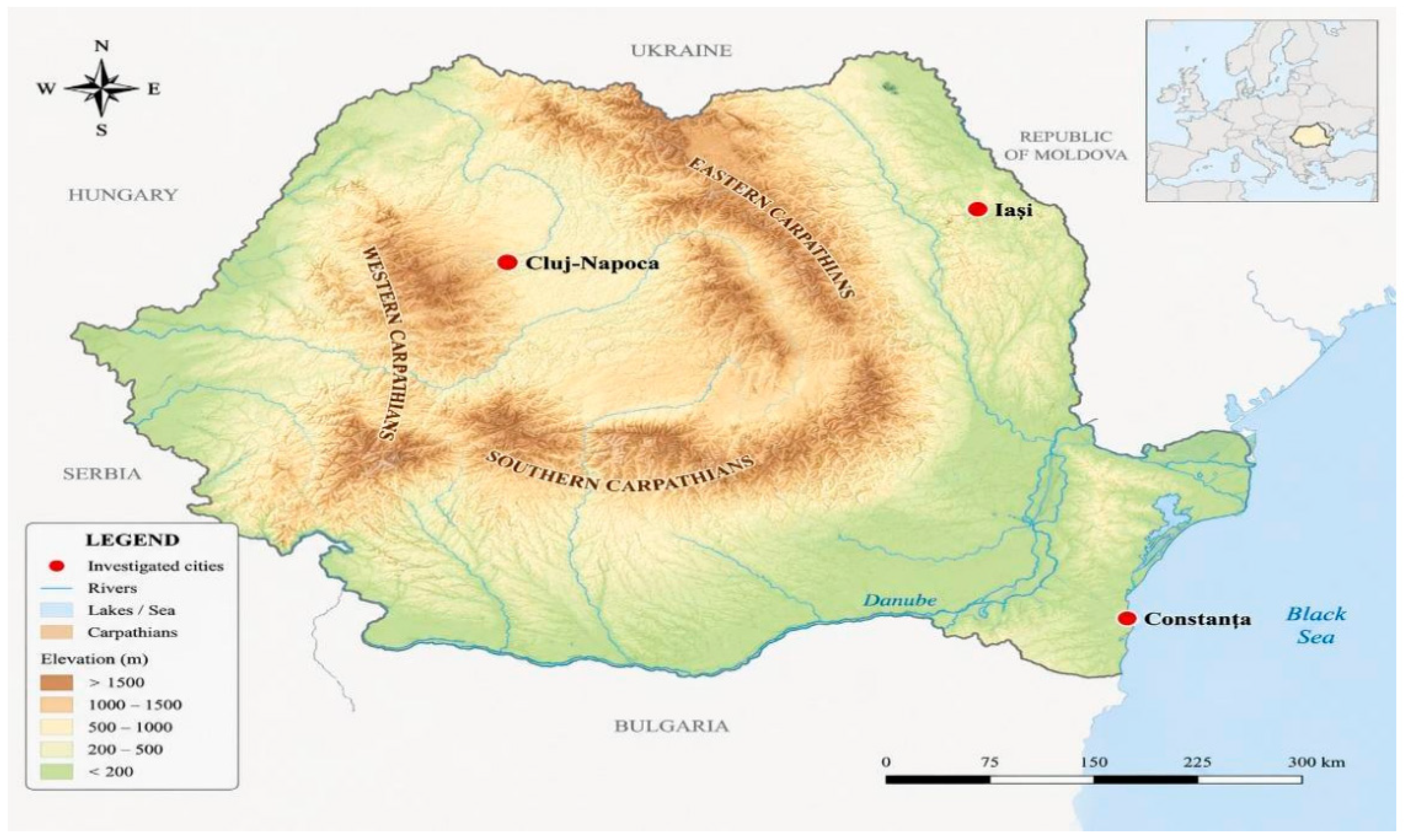
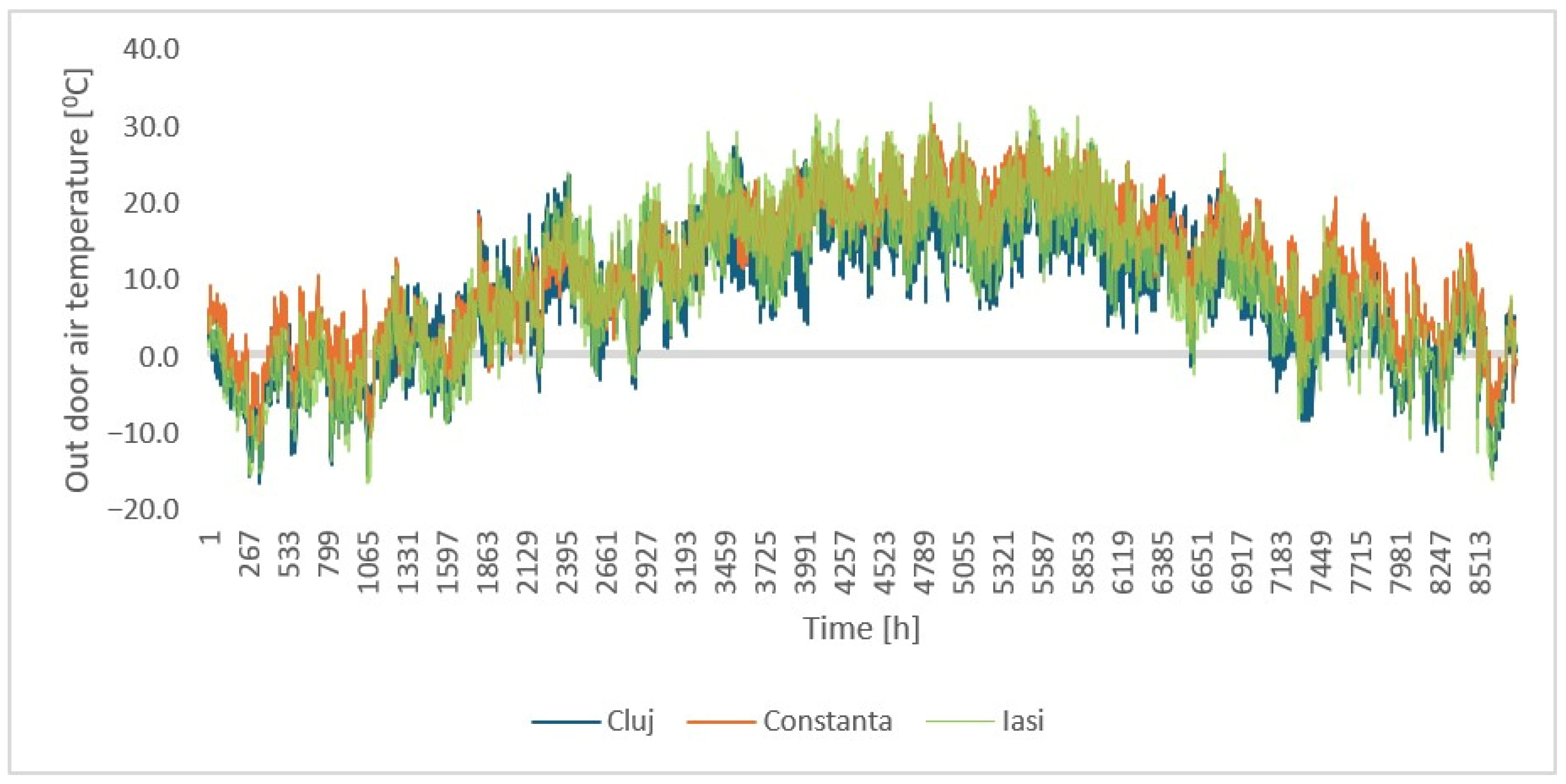
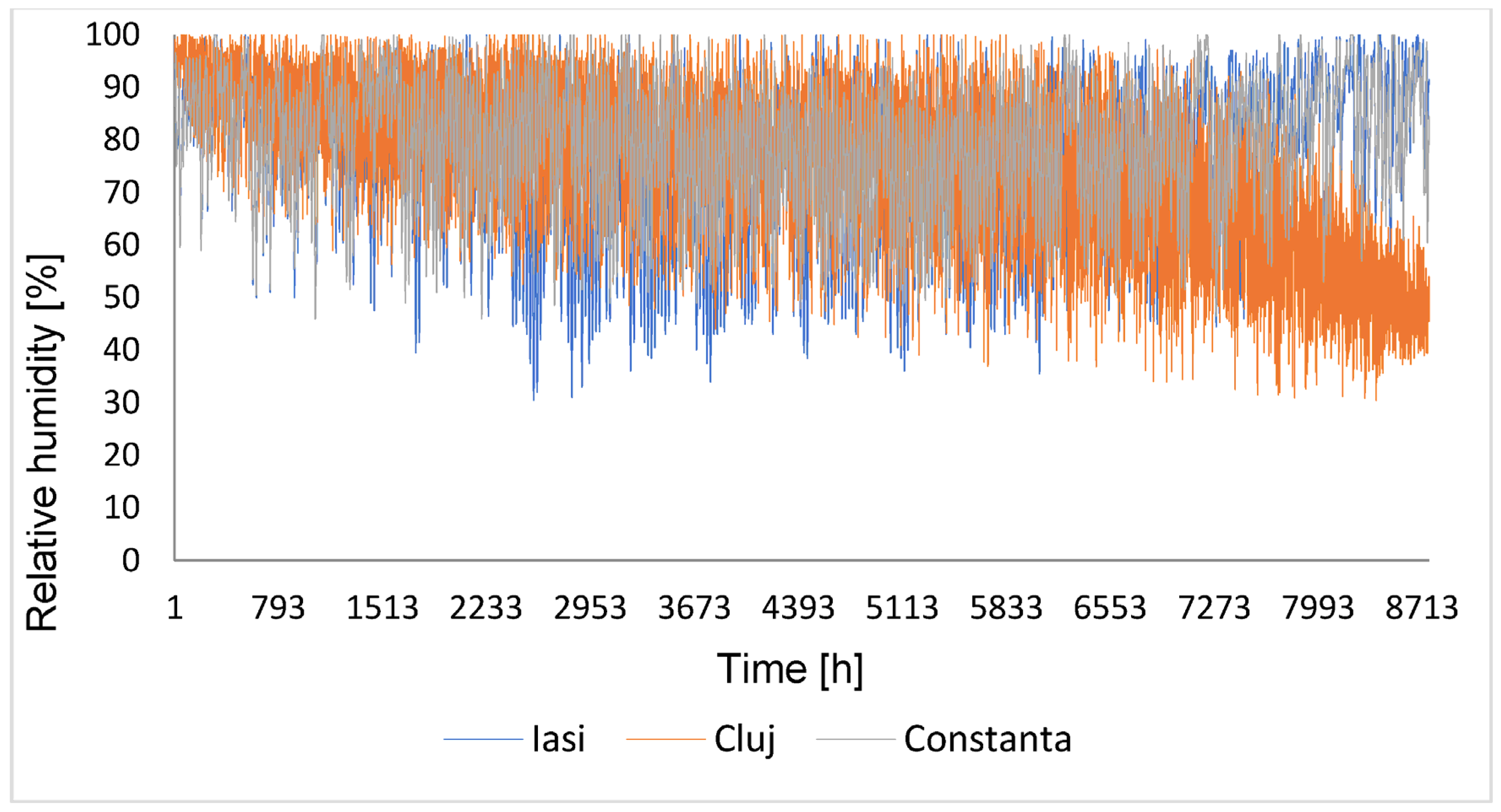
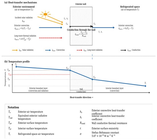
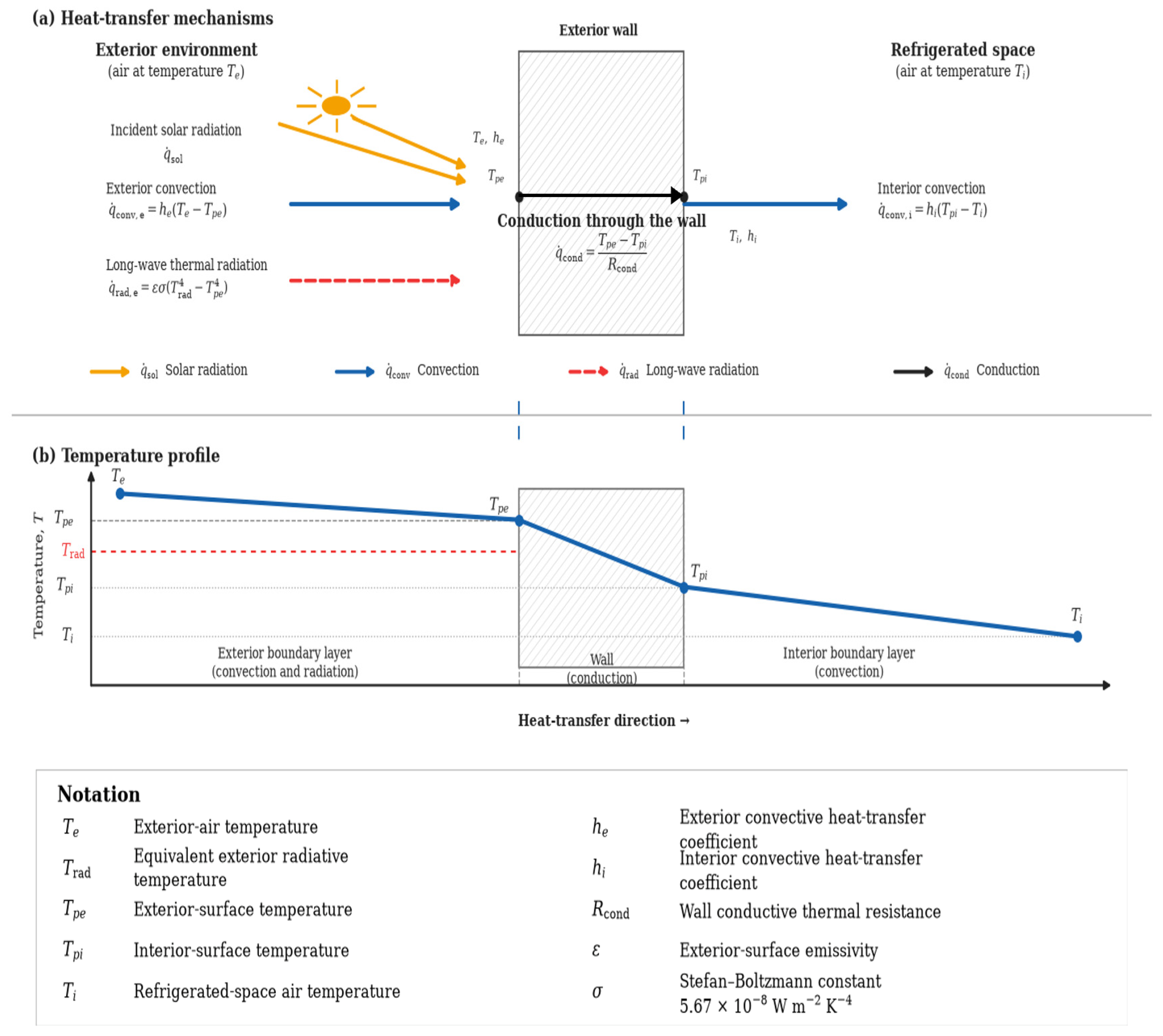
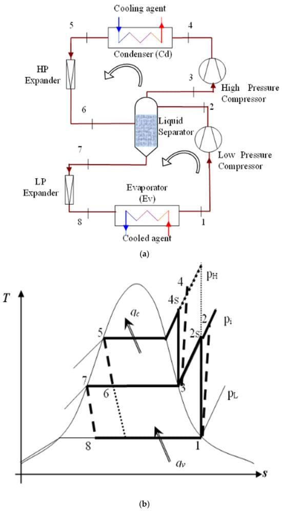
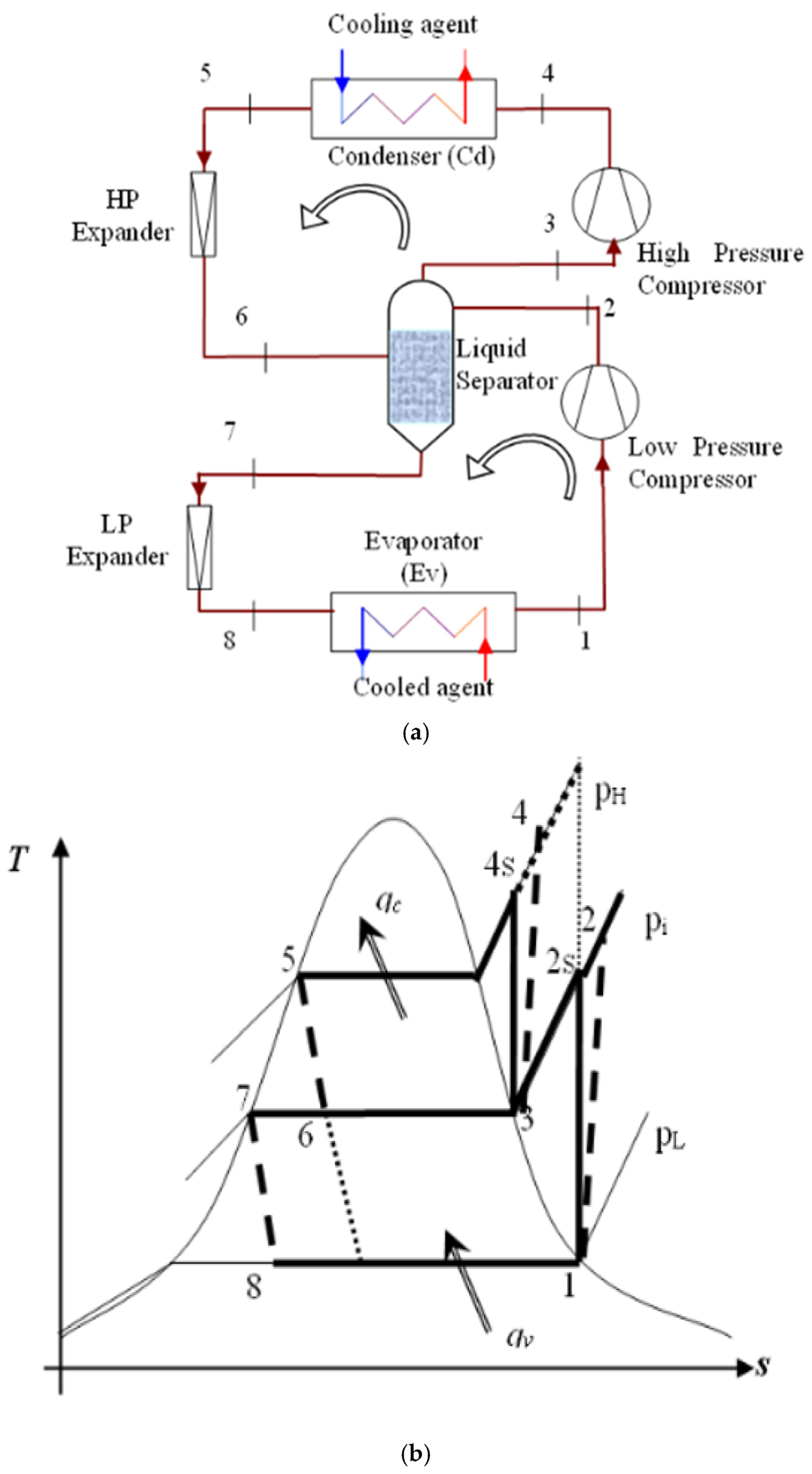
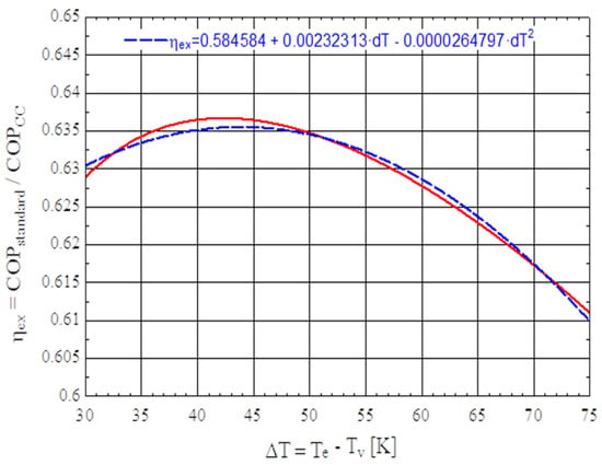
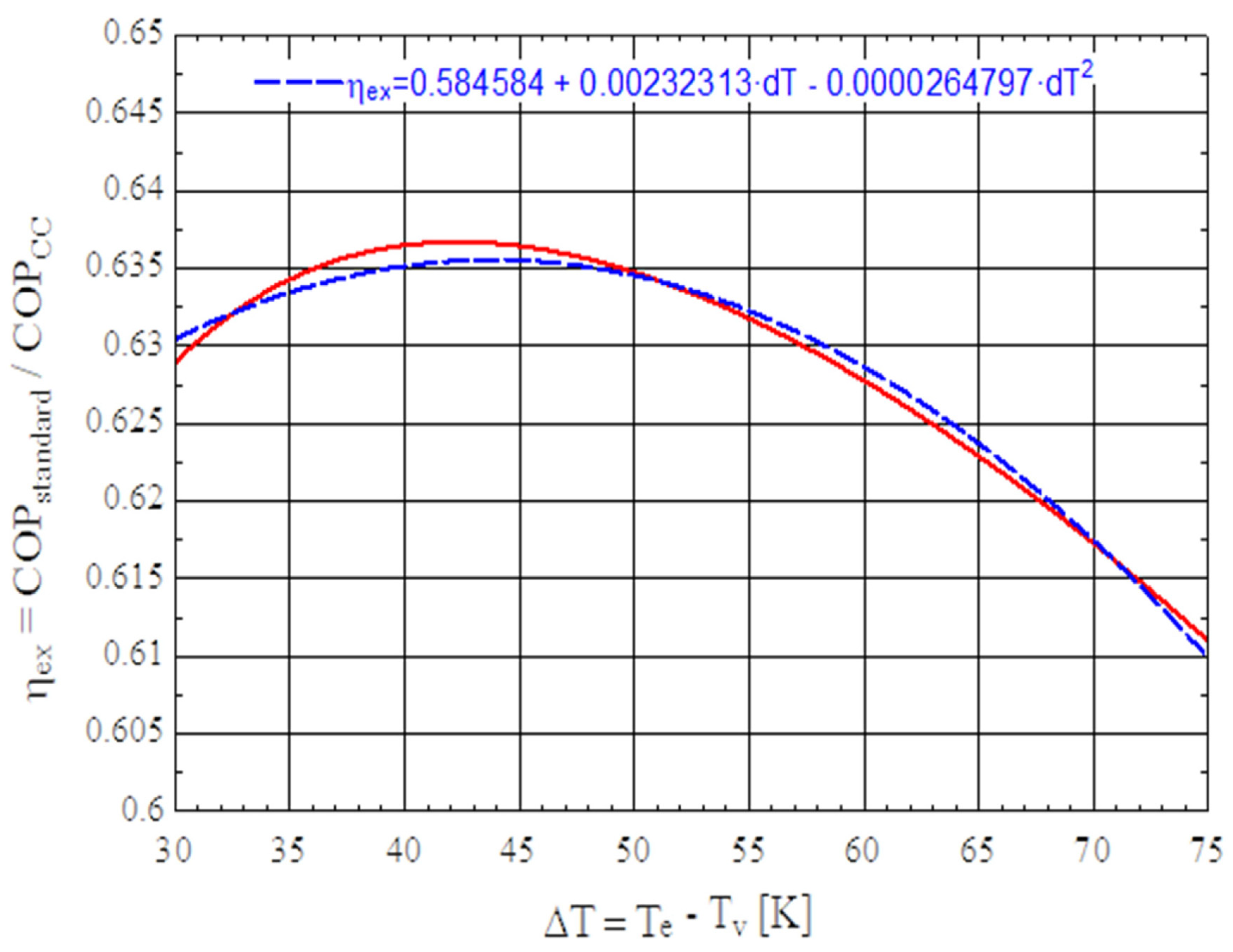
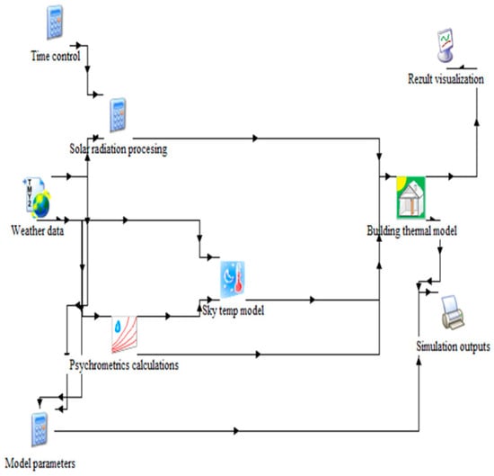
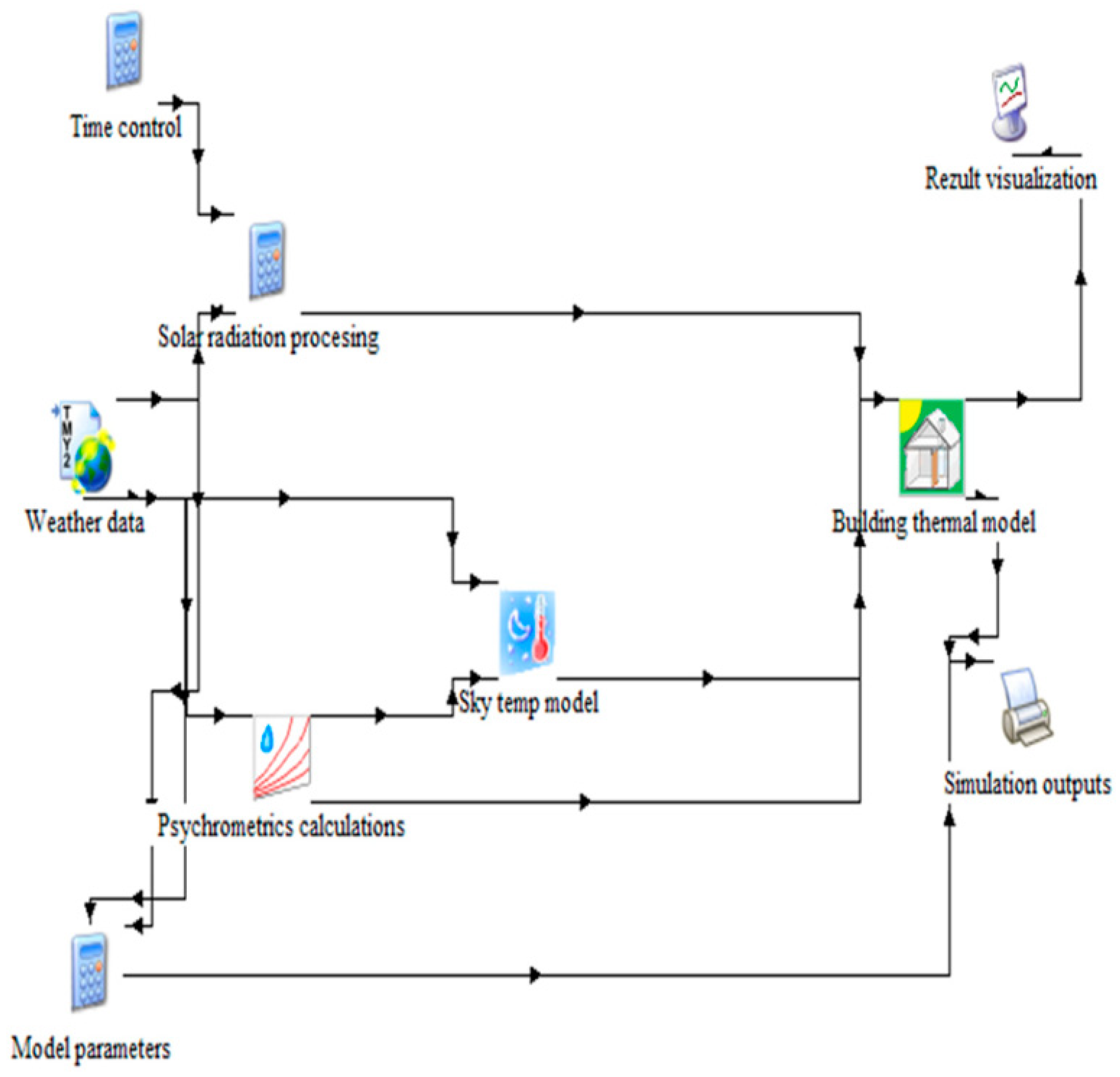
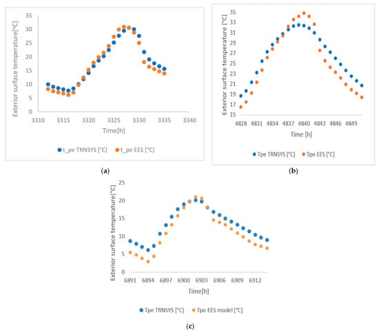
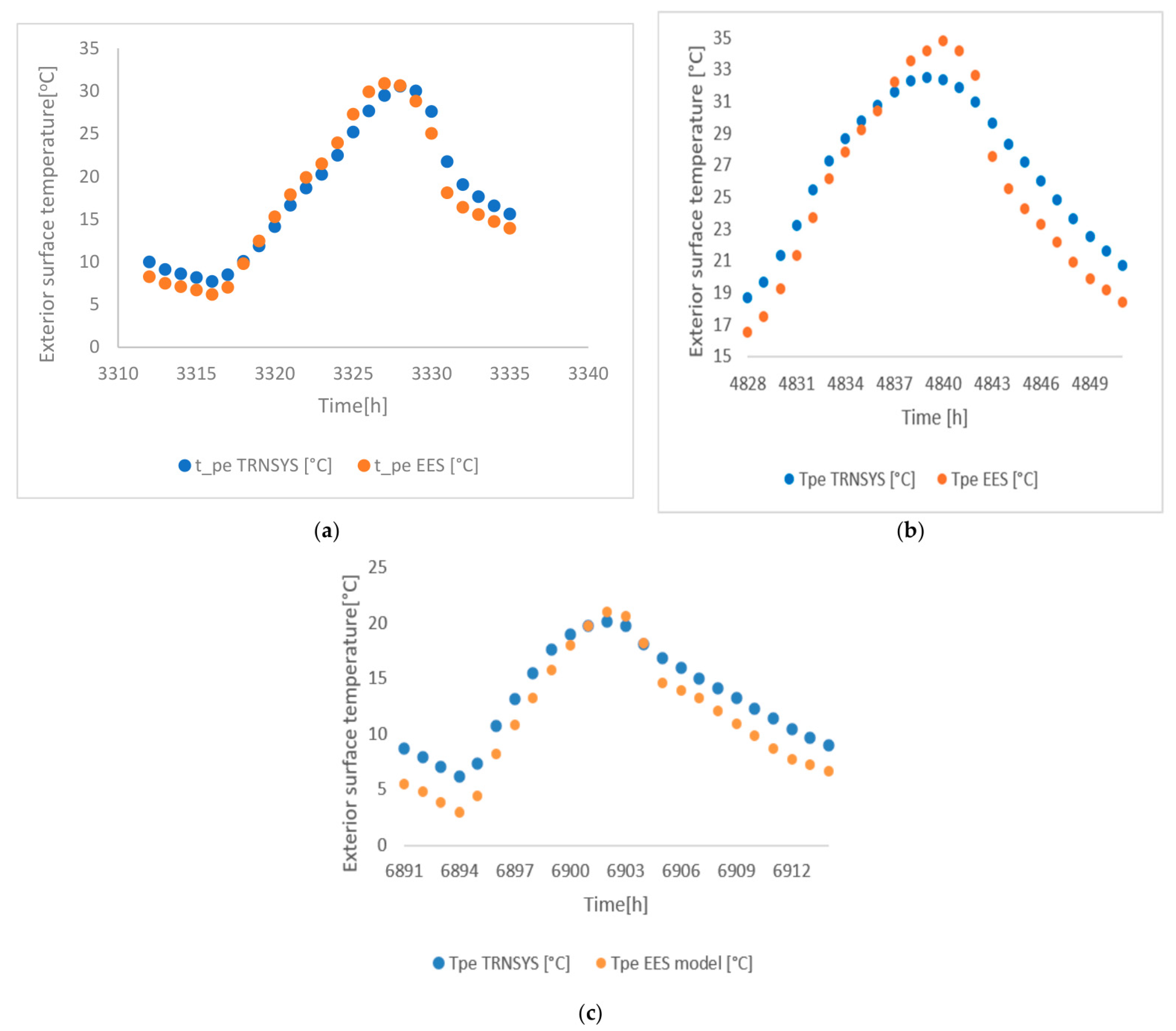
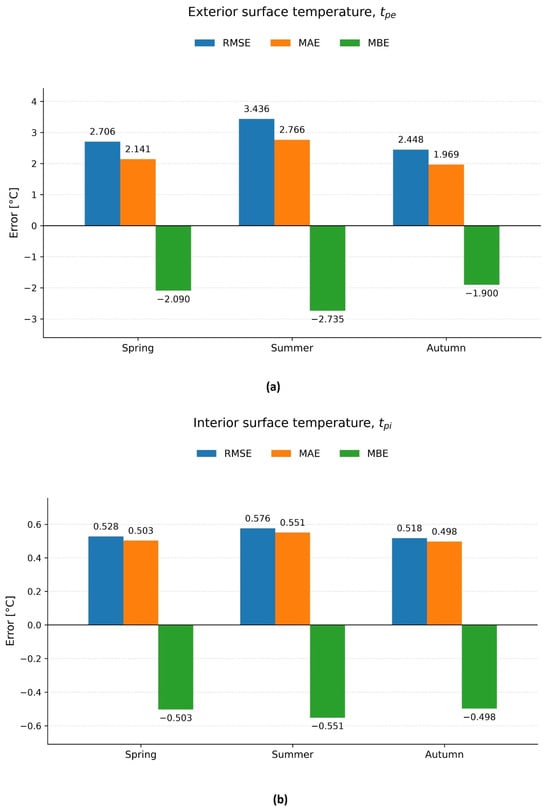
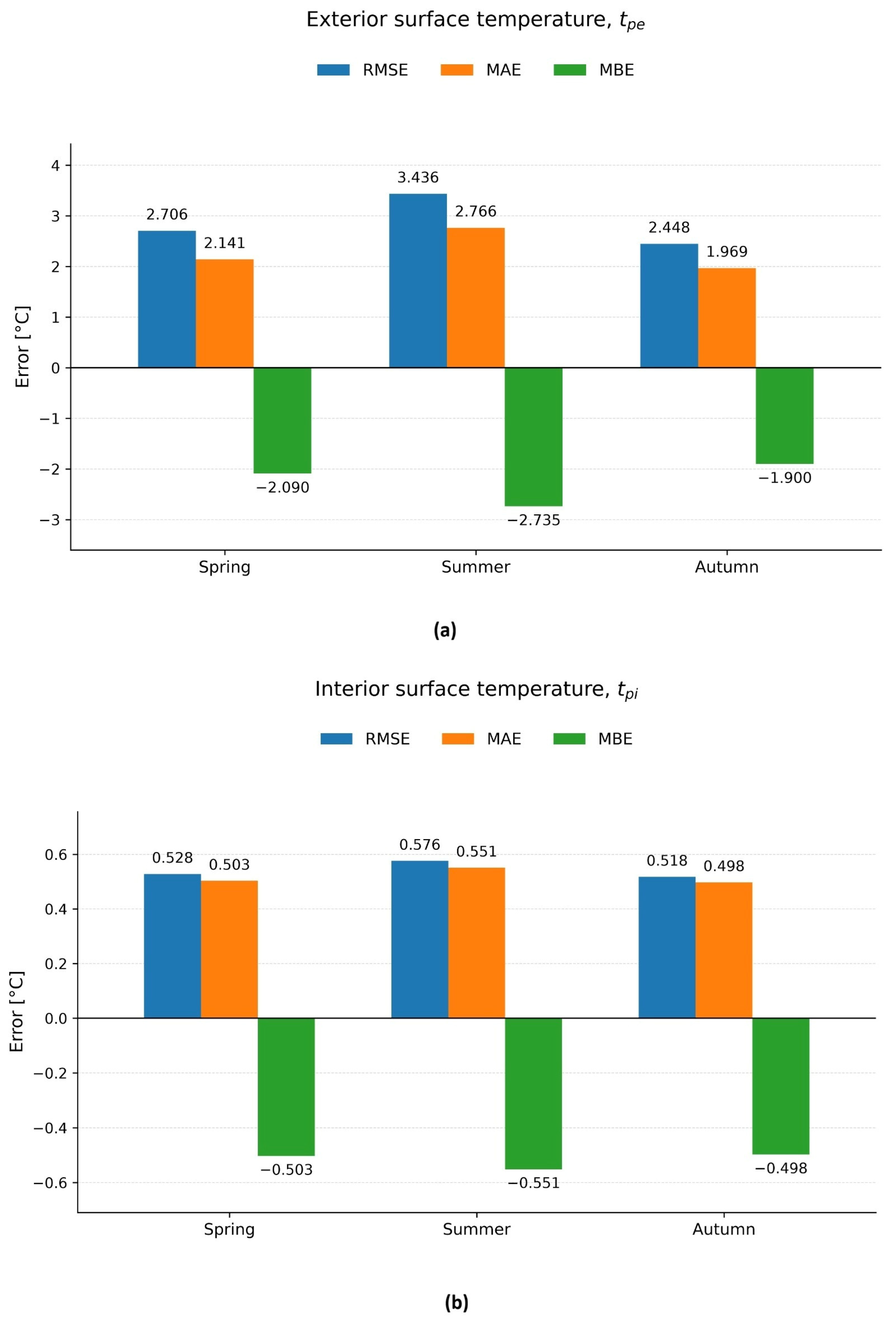
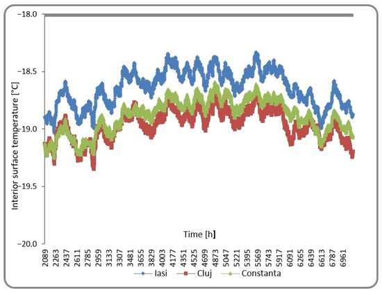
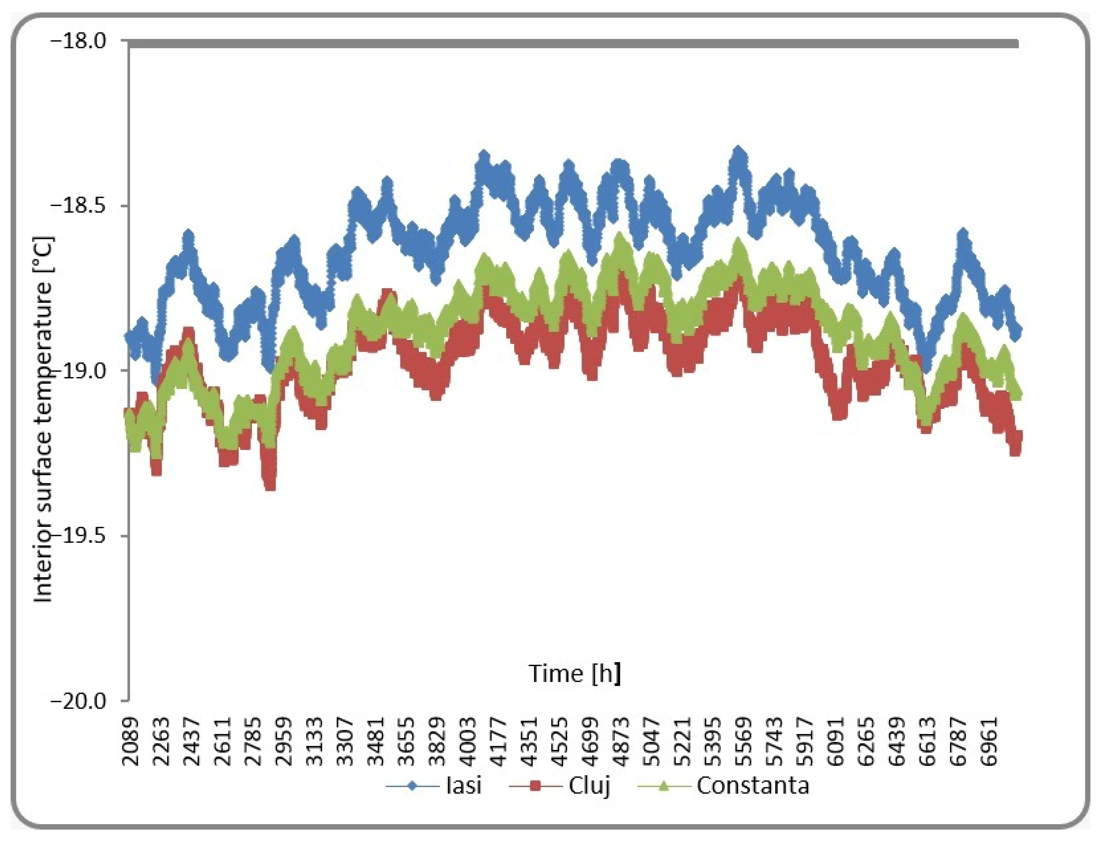
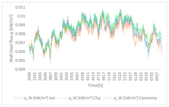
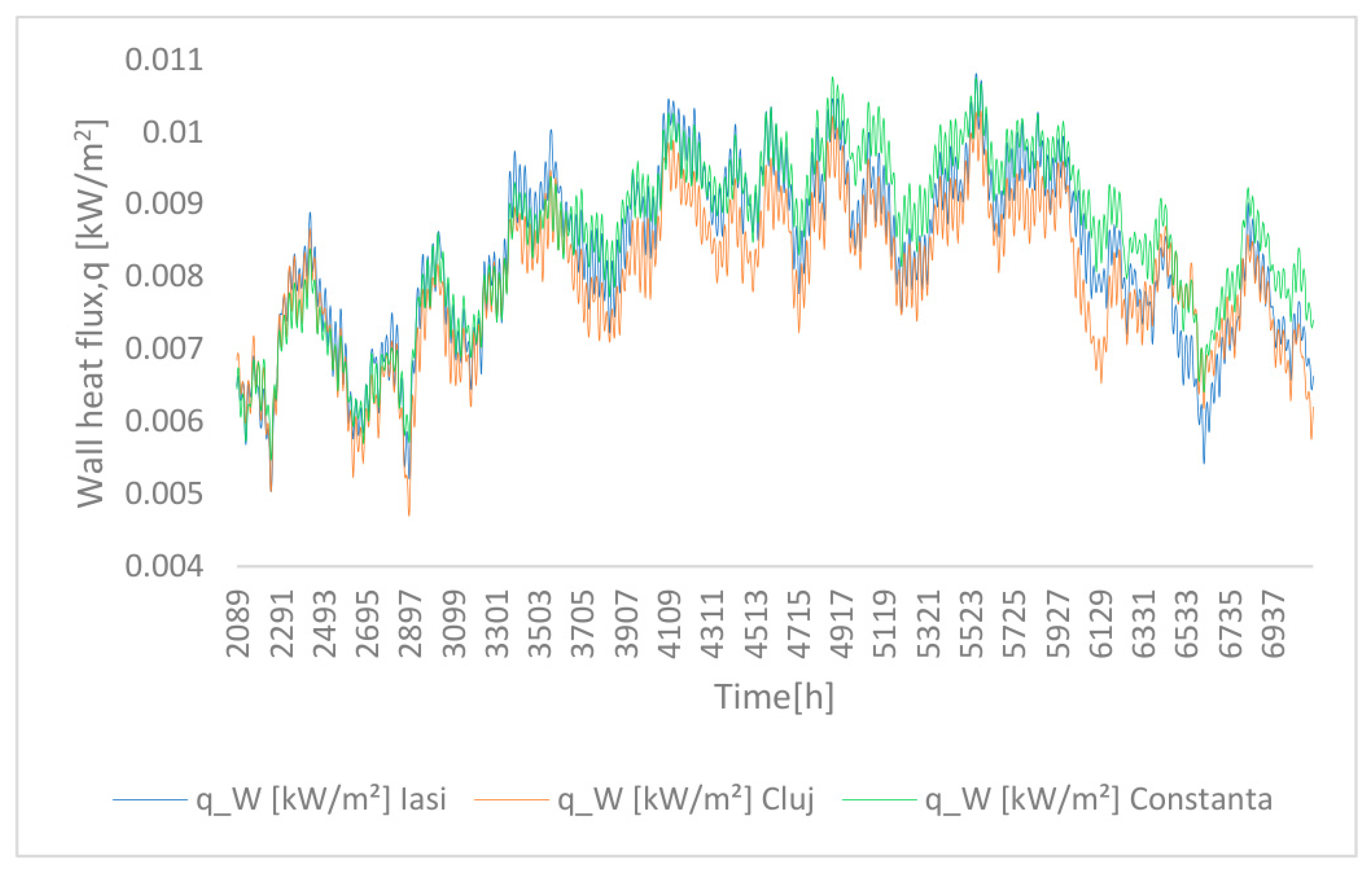
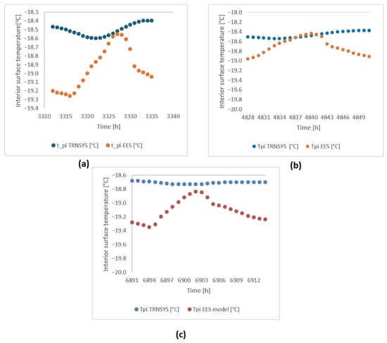
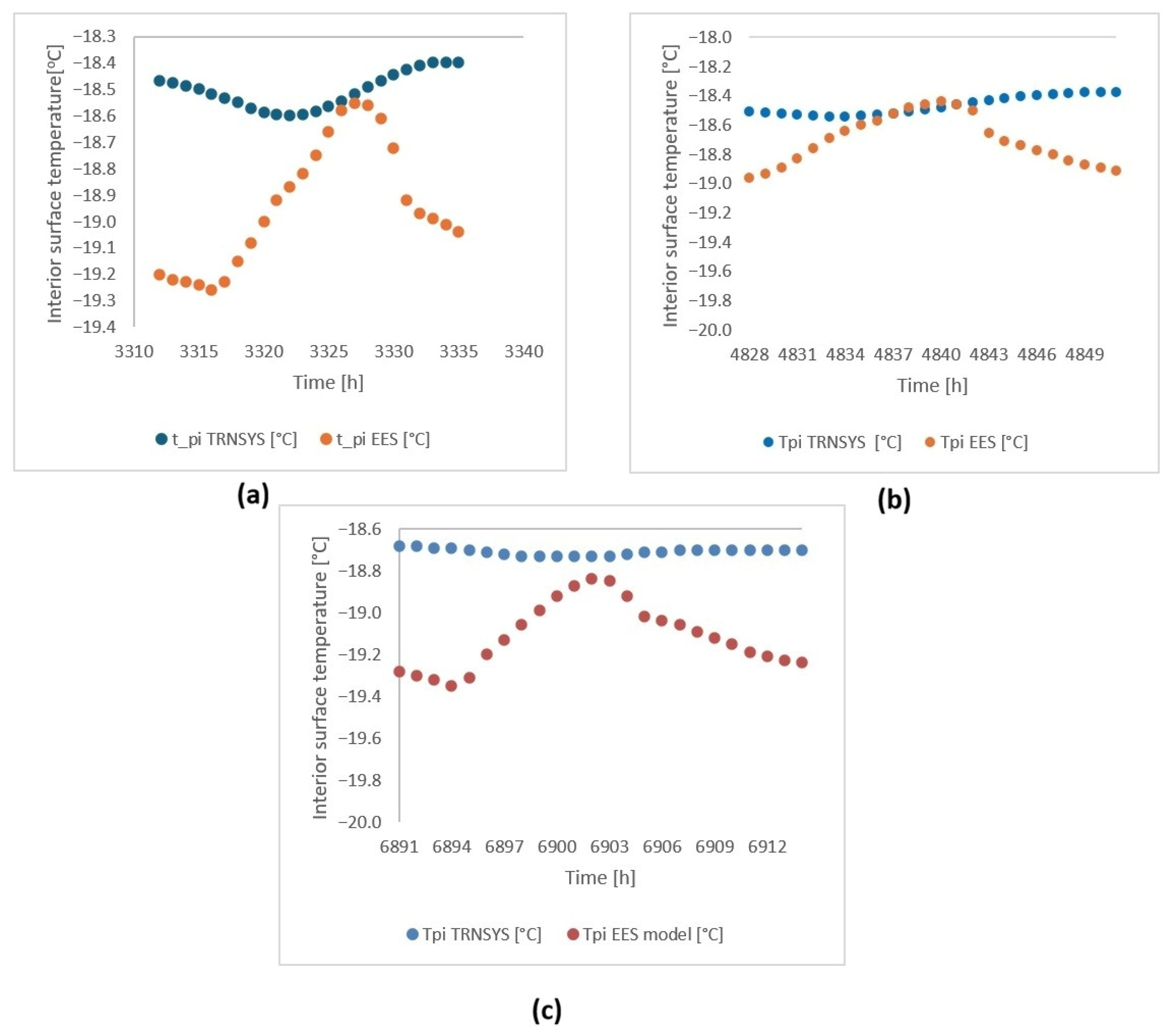
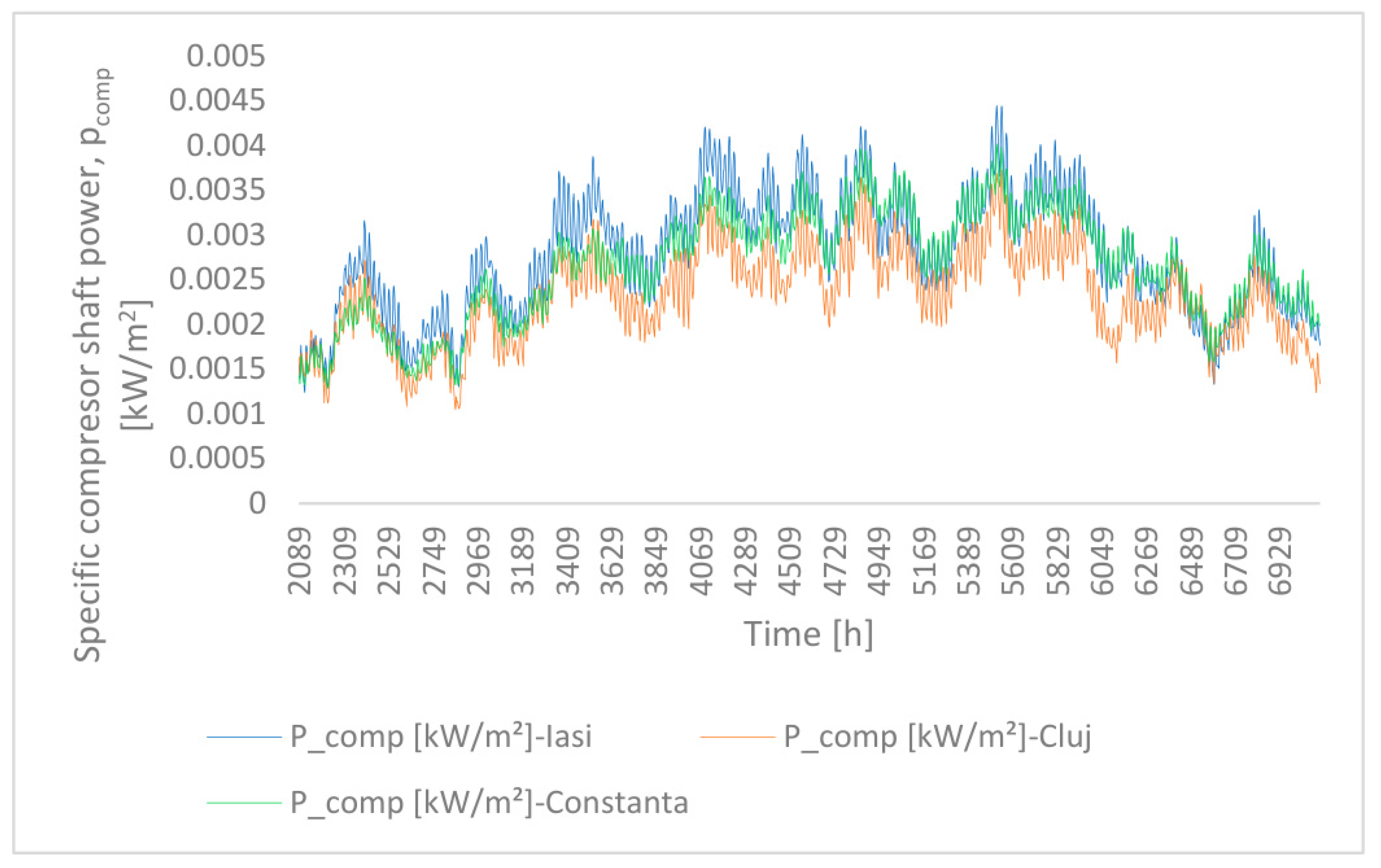
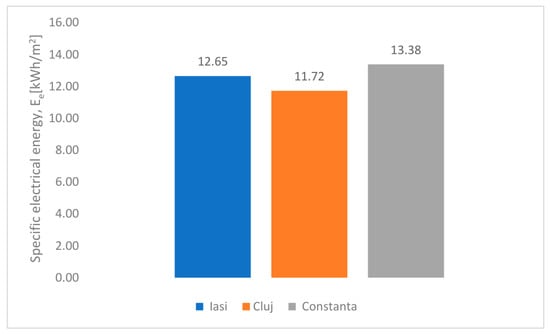
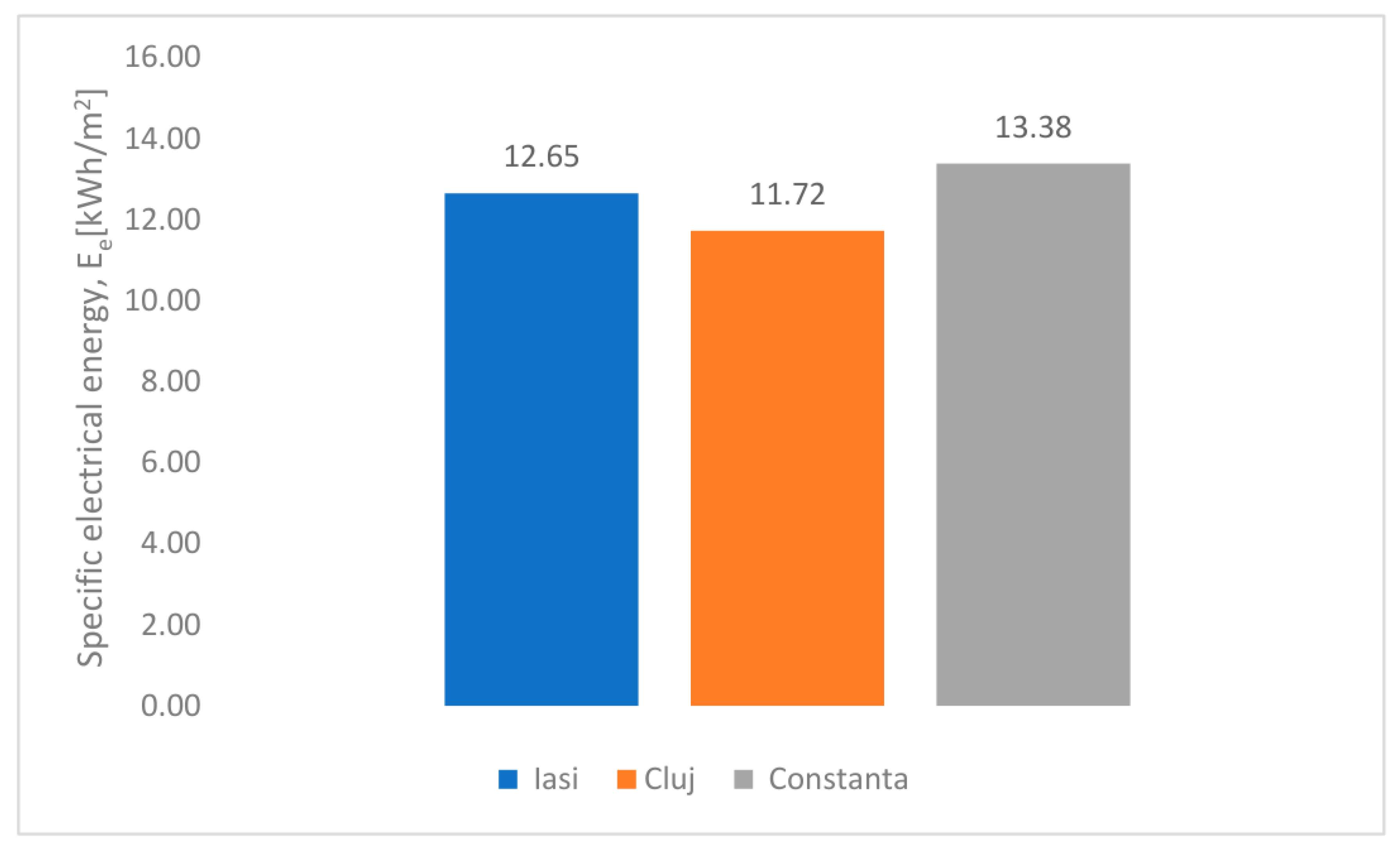

Disclaimer/Publisher’s Note: The statements, opinions and data contained in all publications are solely those of the individual author(s) and contributor(s) and not of MDPI and/or the editor(s). MDPI and/or the editor(s) disclaim responsibility for any injury to people or property resulting from any ideas, methods, instructions or products referred to in the content. |
© 2026 by the authors. Licensee MDPI, Basel, Switzerland. This article is an open access article distributed under the terms and conditions of the Creative Commons Attribution (CC BY) license.