


Abstract
This study presents a developed and characterized Simulink model of an off-grid hybrid photovoltaic (PV) and wind electric vehicle (EV) charging station and characterizes the performance of a rule-based energy management strategy (EMS) that coordinates its four power branches. Predominantly techno-economic studies of such architectures have not provided dynamic models sufficiently to characterize transient behavior, mode transitions, or control limitations. The model integrates a 78.1 kW PV array, a 20 kW wind turbine, a 150 kWh energy-storage unit, and a 25 kW EV port on a regulated 600 V DC bus. Each subsystem is characterized in isolation; the integrated system is exercised under a 50 s four-window stepped-irradiance scenario. During high- and low-irradiance windows, the EMS coordinates all four branches successfully, with bus voltage regulated within ±7 V of a +3.7% steady-state offset. At the intermediate-irradiance window, the filtered PV power oscillates across the hysteresis band, producing 74 charge/discharge transitions in 10 s and sub-millisecond bus voltage transients reaching 903 V, exceeding the 750 V safety threshold. Remediation experiments show that a 50 ms debounce eliminates the chatter but not the transient, identifying two independent architectural limitations of the rule-based design. The dynamic model and baseline established here inform a companion two-stage distributionally robust optimization (TSDRO) controller for the same architecture.
1. Introduction
The transition from internal combustion engines to EVs is accelerating globally, driven by climate commitments, falling battery costs, and tightening urban air-quality regulation [1]. Charging infrastructure has tracked this transition unevenly. In urban centers of high-income economies, grid-connected charging networks are scaling rapidly; in rural and developing-country contexts, the underlying grid that would support such networks is either absent or insufficiently reliable. The result is a structural barrier to EV adoption that is not addressed by improvements in vehicle technology alone.
This barrier is particularly acute in the two case-study contexts examined in this work. In Nigeria, sub-Saharan Africa’s most populous nation, approximately 100 million people lack access to reliable electricity [2], with rural electrification gaps persisting across the country’s six geopolitical zones despite a national energy-transition plan targeting 36% renewables by 2030. Techno-economic studies across representative Nigerian cities have established the viability of off-grid renewable generation, with PV/battery systems achieving a levelized cost of electricity in the range of USD 0.16–0.17 per kWh for 2023 deployment and projected to fall below USD 0.10 per kWh by 2029 [2]. In Fiji, an archipelago of approximately 100 inhabited islands, the centralized grid covers only the three main islands (Viti Levu, Vanua Levu, Ovalau), and outer-island communities depend on solar home systems and Department of Energy diesel generators that operate only for a few hours per evening [3]. Independent feasibility analyses for representative Fijian sites have found that fully renewable PV + wind + battery configurations are technically achievable if modest annual capacity shortages are permitted [3].
What both contexts share is the requirement that EV charging infrastructure must, in many siting decisions, be designed to operate without grid connection at all. The architectural question this raises is not whether off-grid renewable charging is feasible—the literature establishes that it is. Still, how should such stations be configured, controlled, and characterized in a way that supports both deployment confidence and the development of higher-performance control strategies? The present study addresses the second part of this question: it establishes a characterized Simulink model and characterizes the performance of a rule-based energy management strategy under representative operating conditions, providing the baseline against which the model-based control strategies developed in subsequent work will be compared.
1.1. The Hybrid PV–Wind Off-Grid Charging Architecture
A hybrid PV–wind generation architecture offers two operational advantages over PV-only or wind-only off-grid generation. First, diurnal complementarity is as follows: PV generation peaks at midday, while wind is often stronger nocturnally and during overcast conditions, reducing the magnitude of generation-load mismatch that the energy-storage system must absorb. Second, there is seasonal complementarity in many geographies: wind resource is often anti-correlated with solar resource at the seasonal scale, smoothing annual generation. Both effects reduce the energy-storage capacity required to meet a given reliability target, lowering capital cost relative to single-source architecture [1,4].
The architecture modeled in this study combines a 78.1 kW PV array, a 20 kW permanent-magnet synchronous-generator (PMSG) wind turbine, a 150 kWh Lithium-ion energy-storage unit, and a 25 kW EV charging port on a regulated 600 V DC bus. The capacity ratio between renewable generation, storage, and load is chosen to reflect a representative off-grid station serving small-vehicle charging traffic at a regional trading hub, with energy storage sized to bridge approximately one full day of typical EV demand under partial-generation conditions. PV-side capacity dominates the generation total, consistent with the techno-economic findings reported for Nigerian and Fijian off-grid systems [2,3].
A DC bus architecture is used rather than an AC bus because all branch sources and loads are inherently DC; an AC bus would impose unnecessary DC–AC–DC conversion stages and the synchronization and reactive-power management overheads associated with AC coupling. The 600 V bus voltage is selected as a compromise between the lower voltage of the Lithium-ion battery (380 V nominal) and the higher voltage that the PV array can deliver at its maximum power point (MPP) without aggressive boost ratios. Most of the closely related hybrid PV–wind EV charging literature has focused on grid-connected variants of this architecture [4]; the off-grid variant studied here introduces additional control challenges arising from the absence of an external voltage reference and the consequent requirement that the energy-storage branch must establish the bus voltage in its own right.
1.2. The Energy Management Problem
Coordinating the four branches—PV maximum power point tracking (MPPT), wind MPPT, battery charge/discharge, and EV charging—through transitions in generation availability and load is the core control problem of any hybrid off-grid charging station. The dominant approaches partition broadly into rule-based strategies, which select among a small set of operational modes based on instantaneous or filtered measurements, and model-based strategies, which compute control actions from an internal model of system dynamics under uncertainty.
Rule-based strategies are widely adopted in practice for their simplicity, transparent failure modes, and modest computational requirements. Their limitations are also well-established: they typically rely on per-branch calibration at nominal operating points, lack coordination across branches during mode transitions, and offer no formal accommodation of forecast uncertainty in renewable generation [1]. Model-based strategies, by contrast, can deliver coordinated branch control, account for forecast uncertainty, and provide stability guarantees under specified disturbance bounds but require validated dynamic models of the underlying system and a comparison baseline against which their performance can be evaluated.
The present study provides this comparison baseline. A complete dynamic model of the off-grid hybrid PV–wind EV charging station is developed in Simulink. Each subsystem is characterized in isolation, and the integrated system is exercised under a representative scenario with a rule-based two-mode energy management strategy that coordinates the battery charge and discharge controllers. The performance of this rule-based baseline is documented in detail, including the limitations that motivate the development of a two-stage distributionally robust optimization (TSDRO) model-based controller in subsequent work.
1.3. Contributions
This study makes the following specific contributions:
- A complete, characterized Simulink model of an off-grid hybrid PV–wind EV charging station integrating a 78.1 kW PV array, a 20 kW PMSG wind turbine, a 150 kWh Lithium-ion battery, and a 25 kW EV charging port on a regulated 600 V DC bus.
- Subsystem-level characterization of each branch: PV current–voltage (I–V) and power–voltage (P–V) curves at five irradiance levels and P–V curves at three cell temperatures; wind-branch power-duty cycle (P-D) characteristic on a 30-point steady-state grid; and wind-branch perturb-and-observe (P&O) MPPT transient response under a stair-step wind-speed profile.
- A rule-based, hysteresis-based two-mode energy management strategy coordinating the battery charge and discharge controllers, with full specification of mode thresholds, filter design, and safety overrides.
- Quantitative assessment of integrated-system performance under a four-window (W1–W4) characterization scenario, with per-window analysis of DC bus regulation, mode-transition behavior, branch power flows, and battery state-of-charge trajectory.
- Identification of specific architectural limitations of the rule-based baseline, including bus regulation offset, mode-transition transients, and dual-regime wind tracking, that motivate the model-based control strategies pursued in companion work.
2. Related Work
The technical literature on off-grid hybrid PV–wind charging systems sits at the intersection of five established research areas: techno-economic feasibility analysis of off-grid hybrid renewable systems in developing-country contexts; dynamic modeling of hybrid PV–wind power systems; DC microgrid bus regulation and converter control; rule-based and model-based energy management strategies for multi-source DC microgrids; and EV charging infrastructure modeling. The present study draws on each area and contributes a baseline, characterized Simulink model that combines all four branches (PV, wind, battery, EV) in a single off-grid topology with full controller-level disclosure and rule-based EMS coordination, extending prior dynamic-modeling work that has predominantly addressed grid-connected variants.
2.1. Off-Grid Hybrid Renewable Systems in Developing-Country Contexts
The dominant literature on off-grid hybrid renewable systems in developing-country contexts is techno-economic in orientation, typically using HOMER Pro or equivalent simulation environments to evaluate annual energy delivery, levelized cost of electricity, and renewable-fraction metrics across candidate system sizing. Representative country-specific studies include the Nigerian techno-economic studies across the country’s six geopolitical zones [2]; broader sub-Saharan Africa surveys [5]; the Nabouwalu (Vanua Levu, Fiji) feasibility analysis of Lal and Raturi [3]; and analogous studies for rural electrification contexts in other sub-Saharan African countries, the Pacific Islands, and Latin America [6,7,8]. The HOMER software environment itself, originally developed at the U.S. National Renewable Energy Laboratory [9], has become the de facto standard for techno-economic feasibility analysis of off-grid hybrid systems.
These studies establish that off-grid hybrid configurations are technically and economically viable across the geographies of interest to this study, with PV-dominant configurations achieving levelized costs below USD 0.20 per kWh in current deployment and projected to decline further with continued battery and module cost reductions [2]. The role of wind generation in such hybrid configurations is generally smaller than PV but contributes meaningfully to inter-day and seasonal energy balancing where the local wind resource is consistent [10,11]. Battery storage capacity sizing is treated extensively in the techno-economic literature, with several authors developing optimization frameworks for joint generation-storage sizing under uncertain load forecasts [12,13]. What the literature does not provide, however, is the dynamic-system model required to characterize transient behavior, control responses, or stability margins of the candidate architectures. The present study complements the techno-economic work by providing exactly such a model for a specific off-grid hybrid PV–wind EV charging architecture.
2.2. Dynamic Modeling of Hybrid PV–Wind Systems
A distinct strand of the literature has developed Simulink and equivalent dynamic-system models of hybrid PV–wind architectures. Foundational work on the PV side includes the widely used single-diode module model [14] and its derivatives [15], together with characterizations of boost-converter MPPT algorithms, including the P&O family [16], incremental-conductance variants [17], and more recent machine-learning-based approaches [18]. On the wind side, the textbook of Heier [19] provides the standard turbine aerodynamic formulation used in the present study, complemented by detailed treatments of PMSG modeling [20] and PMSG–rectifier–boost chain dynamics [21].
The closest published analogue to the present study’s architecture is the grid-connected PV–wind EV charging system of Tharwin Kumar and Asir Rajan [4], which models a similar four-branch configuration but with a stiff AC grid providing the bus voltage reference. Related grid-connected dynamic-modeling work includes integrated PV–wind battery systems for residential and commercial charging [22,23] and DC fast-charging station models with photovoltaic supplementation [24,25]. The grid-connected variant has been the dominant focus of dynamic-modeling work in this area because grid-connected operation simplifies the bus-voltage regulation problem: the grid provides an external voltage reference, and the energy-storage branch’s role reduces to power-balance management. The off-grid variant studied here introduces additional control challenges arising from the absence of an external voltage reference, including the structural requirement that the energy-storage branch must itself establish the DC bus voltage through its own controller dynamics. The review article by Ibezim et al. [1] surveys this literature in detail and identifies the off-grid dynamic-modeling case as an open area of work.
2.3. DC Microgrid Bus Regulation and Converter Control
A separate body of work addresses the bus regulation problem in DC microgrids more generally, independent of the specific generation or load technology. Droop control on the DC bus has been studied extensively as a means of distributing power flow among multiple source converters without explicit communication [26,27] with extensions to adaptive droop strategies [28] and consensus-based distributed control [29]. The bidirectional buck/boost converter used in the present study’s energy-storage branch is a standard topology in the literature [30], with several recent papers proposing improved control strategies, including sliding-mode control [31], predictive control [32] and observer-based disturbance rejection [33].
Stability analysis of DC microgrids with multiple constant-power loads, including EV chargers, has received particular attention because constant-power loads can destabilize an otherwise-stable bus through their negative incremental impedance [34,35]. The present study’s architecture, with the EV branch implementing a constant-current then constant-voltage charge profile, exhibits constant-power load behavior during the constant-current phase; the bus regulation strategy must, therefore, be robust to this loading characteristic.
2.4. Energy Management Strategies in Renewable DC Microgrids
Energy management strategies for multi-source DC microgrids partition broadly into rule-based and model-based approaches. Rule-based strategies—typically implemented as finite-state machines with hysteresis on filtered measurements—are the predominant choice in deployed off-grid systems for their simplicity, transparent failure modes, and modest computational requirements [1,36,37]. The principal limitations of rule-based designs documented in the literature include their reliance on per-branch calibration at nominal operating points, the lack of explicit coordination across branches during mode transitions, and the absence of any formal treatment of forecast uncertainty in renewable generation or load [38].
Model-based strategies promise improved coordination and explicit accommodation of uncertainty. Model-predictive control has been applied extensively to DC microgrid EMS problems [39,40], with formulations addressing both deterministic and stochastic disturbance models. Robust control approaches address worst-case disturbance bounds [41], while distributionally robust optimization (DRO) approaches hedge against ambiguity in the disturbance distribution itself [42,43,44]. Two-stage DRO formulations—in which a first-stage decision is made before disturbances are realized, and a second-stage decision is optimized over the worst-case distribution within an ambiguity set—have recently been applied to renewable-energy scheduling problems [45]. These approaches require both validated dynamic models of the underlying system and a rule-based baseline against which their performance can be evaluated. The present study provides this rule-based baseline; the companion work develops a two-stage DRO controller for the same architecture using the baseline characterization reported here as its comparison reference.
2.5. EV Charging Infrastructure and Renewable Integration
The integration of EV charging infrastructure with renewable energy sources has been studied extensively, primarily in grid-connected contexts. Standard constant-current (CC)–constant-voltage (CV) charging profiles for Lithium-ion batteries are well-characterized [46,47] and have been integrated into power-electronic charger designs [48]. Recent work has examined the techno-economic case for solar-powered EV charging in various geographies [49,50], with particular emphasis on workplace and parking-lot deployments. Off-grid EV charging, in which the entire energy supply chain operates without grid connection, remains a less-developed area of the literature [51], particularly for cases that combine multiple renewable sources with on-site storage to support charging across periods of low generation. The present study addresses this less-developed case directly.
3. System Model
3.1. System Architecture
The off-grid hybrid charging station modeled in this study consists of four power branches sharing a regulated 600 V DC bus, as shown in Figure 1. The renewable-generation branches comprise a 78.1 kW PV array, with 20 parallel strings of 13 series-connected Suntech STP300-24/Vd modules, and a 20 kW horizontal-axis wind turbine driving a permanent-magnet synchronous generator with three-phase passive rectification. The storage branch is a 150 kWh Lithium-ion energy-storage unit (ESU) at a nominal 380 V battery-side voltage, interfaced to the bus through a bidirectional buck/boost converter. The load branch is a single 25 kW EV charging port at a nominal 360 V EV-battery-side voltage, interfaced through a buck converter operating in CC then CV modes.
Figure 1.
System architecture of the off-grid hybrid PV–wind EV charging station baseline.
Each branch interfaces with the common bus through its own dedicated DC–DC power-electronic converter, allowing each branch to be characterized independently of the others. The PV and wind boost converters are each driven by their own P&O MPPT (see Section 5.1 and Section 6.1). The ESU bidirectional stage is split into two controllers, one for charging and one for discharging, with a single rule-based energy management strategy selecting which is active (see Section 7.2). The EV buck converter implements a CC charging profile when the EV is connected. DC bus filtering is provided by a bus-side capacitor common to all four branches. There is no AC-side coupling in the architecture; all power flow is DC throughout, which simplifies the converter topology and eliminates the synchronization and reactive-power requirements that would otherwise be imposed by an AC-side common bus.
The architecture’s nominal operating point is 600 V at the DC bus. Switching frequencies are 20 kHz for the PV-side boost converter and 10 kHz for the wind-side boost converter; the ESU and EV-side converters share the 20 kHz rate. The numerical sample time of the simulation is set by these switching dynamics and is fixed at Ts = 5 × 10⁻⁶ s throughout.
3.2. Solver and Numerical Settings
All simulations reported in this work were run in MATLAB/Simulink R2024b (The MathWorks, Inc., Natick, MA, USA) with the fixed-step ode4 (Runge–Kutta) integrator at a sample time of Ts = 5 × 10⁻⁶ s. This step size is set by the fastest sample-time requirement in the model, which is the 5 µs internal sample time of the three-phase Universal Bridge and the PWM sawtooth generators driving the four DC–DC converters; running the rest of the model at a larger step would force the converter dynamics to be aliased. Variable-step solvers were evaluated during early development and rejected, as the discontinuous switching events of the PWM blocks produced excessive zero-crossing detection load and severely degraded wall-clock performance. With the fixed-step configuration adopted here, a 50 s integrated simulation completes in approximately 22 min of wall-clock time on a standard workstation.
The converter and DC-bus component values that determine the model’s transient behavior are summarized in Table 1. Because this study’s principal findings concern fast converter and bus-voltage transients, these values are reported in full to support reproducibility. The four DC–DC converters share a common inductor–capacitor topology but differ in their component ratings and switching rates: the PV boost, bidirectional battery, and EV buck converters each switch at 20 kHz, while the wind boost converter switches at 10 kHz, a deliberate design choice reflecting the lower dynamic bandwidth required at the wind branch’s operating power. The PV and wind boost inductors are modeled as ideal (lossless) inductors, while the battery and EV converter inductors include a 1 mΩ series resistance; small line resistances (10 mΩ wind, 50 mΩ EV) are included on the respective branches. The DC bus is stabilized by a 5 mF bus capacitor initialized at the 600 V reference.
Table 1.
Converter and DC-bus parameters used in the integrated-system model.
Three distinct timescales govern the discrete-time implementation and should be distinguished, since a single 5 µs step is not used across all simulations. First, the solver step is the fixed-step ode4 integration period. In the integrated-system scenario (Section 9), where fast bus-voltage and mode-transition transients are the object of study, it is set to Ts = 5 µs, matched to the fastest sample-time requirement in the model (the internal sample time of the three-phase Universal Bridge and the PWM carriers). In the steady-state wind-branch P–D sweep (Section 6.2), where only the time-averaged delivered power at each operating point is measured, and no fast transient is resolved, a coarser solver step of 50 µs is used to reduce the wall-clock cost of the 30-point sweep without affecting the steady-state results Second, the PWM switching periods are 50 µs for the 20 kHz converters and 100 µs for the 10 kHz wind converter, realized as sawtooth carriers compared against each converter’s commanded duty cycle. Third, the control sampling periods at which the discrete controllers update their duty-cycle commands are not uniform: the boost, charge, and discharge controllers update at the 5 µs solver step, whereas the EV charging controller updates at 50 µs—ten-times the base solver step—which is sufficient for the seconds-scale CC-CV charging dynamics.
4. Simulation Setup and Characterization Protocol
The Simulink model in Section 3 was exercised through four subsystem characterization activities and one integrated-system scenario. The subsystem activities, presented in Section 4.1, comprise a static evaluation of the PV branch’s I–V and P–V characteristics, a 60 s pre-integration run of the standalone PV + ESU + EV configuration, a 30-point steady-state sweep of the wind branch’s P–D characteristic, and a stair-step transient characterization of the wind branch’s P&O MPPT. The integrated-system scenario, presented in Section 9.1, exercises all four branches together over 50 s under the rule-based EMS. Per-window data extraction is described in Section 4.2.
4.1. Subsystem Characterization Runs
The PV branch was characterized using two distinct activities. First, the array’s electrical characteristics were generated using the Simulink PV array block’s built-in characteristic display function, which evaluates the single-diode module model analytically over the voltage range [0, Voc] at user-specified irradiance and temperature operating points. Two characteristic sets were produced: I–V and P–V curves at five irradiance levels (200, 400, 600, 800, 1000 W/m2) under the standard test temperature (25 °C), and P–V curves at three cell temperatures (25, 45, 60 °C) under standard irradiance (1000 W/m2). These curves represent the steady-state electrical characteristics of the array as defined by the module model and do not include converter or system dynamics; they are reported in Section 5.2. Second, the standalone PV + ESU + EV configuration (the pre-wind baseline of Section 5.1) was simulated for 60 s under a stair-stepped irradiance profile compressing a diurnal cycle (1000 W/m2 for the first 30 s, then 500 W/m2 for 10 s, 200 W/m2 for 10 s, and 0 W/m2 for the final 10 s), with the EV connected at t = 1 s and the battery at 50% initial SoC. This simulation exercises the boost converter, MPPT, ESU charge/discharge, and EV CC-CV controllers together but without the wind branch, establishing a pre-integration baseline for the bus voltage and EMS mode behavior.
The wind branch’s P–D characteristic was mapped through a 30-point steady-state parameter sweep over wind speed Vwind ∈ {4, 6, 8, 10, 12, 14} m/s and boost-converter duty cycle D ∈ {0.35, 0.45, 0.55, 0.65, 0.75}. Each combination was simulated for 10 s at constant inputs, with the duty-cycle reference applied as a constant value rather than through the MPPT loop. Steady-state delivered power was averaged over the window t ∈ [3, 10] s, excluding the initial 3 s spin-up transient during which the PMSG rotor reaches its operating angular velocity. To eliminate state carry-over between sweep points, the model was unloaded and reloaded (close_system/load_system) between simulations; the sweep was, therefore, strictly stateless from one Vwind–D pair to the next. Two operating points exhibited extended initial transients near the diode-conduction threshold and required individual re-simulation to confirm steady-state values.
The wind branch’s P&O MPPT response was characterized through a transient simulation with a stair-step wind-speed profile, holding Vwind constant at 8, 10, 12, and then 14 m/s for 5 s per segment, for a total simulation duration of 20 s. The MPPT algorithm operated continuously throughout, perturbing the duty cycle as described in Section 6.1 and producing the rotor-speed and aerodynamic-power-coefficient time series reported in Section 6.3.
4.2. Measurement Points and Data Extraction
The signals logged from each simulation include the following: Vdc (DC bus voltage), Ibatt (battery current, sign convention positive on discharge), battery SoC, the EMS mode indicator, Ppv (PV-side instantaneous power), Pdelivered (wind-branch delivered power at the bus side), and Iev (EV charging current). For the integrated scenario, per-window summary statistics (mean, standard deviation, range) were computed over each operating window, with the first 0.5 s of each window excluded to remove the immediate post-transient. Transient events at scenario boundaries (EV connection at t = 1 s; PV steps at t = 30 s and t = 40 s) are reported with full-time resolution, where their magnitudes inform the discussion in Section 9.3 and Section 9.4.
5. PV Branch Model
5.1. PV Branch
The PV array is implemented as 20 parallel strings of 13 series-connected Suntech Power STP300-24/Vd polycrystalline modules in the Simulink PV array block. In standard test conditions (1000 W/m2, 25 °C), the array delivers a nameplate maximum power of 78.1 kW with an MPP voltage of ~480 V and MPP current of ~163 A. Per-module electrical parameters, array topology, and converter settings are listed in Table 2. The module-level parameters (open-circuit voltage Voc, short-circuit current Isc, voltages and currents at the MPP (Vmp and Imp,), temperature coefficients, and single-diode model parameters) are the supplied defaults from the NREL System Advisor Model preset for this module. The single-diode model formulation itself follows the standard treatment in the literature [14].
Table 2.
PV module and array parameters.
The array interfaces to the 600 V DC bus through a boost converter operating at a 20 kHz switching frequency. The converter is driven by a P&O MPPT [16] that operates in two stages. A feedforward duty cycle Dff = 1 − Vpv/Vdc,ref establishes the open-loop converter operating point using the measured array voltage and the 600 V bus reference. A PI correction with proportional gain Kp = 0.02 and integral gain Ki = 1.0 closes the voltage loop, driving the array operating point to a reference that is itself perturbed by the P&O algorithm. The P&O algorithm samples the array power Ppv = Vpv × Ipv at the converter switching rate, perturbs the voltage reference by a step ΔV, and updates the perturbation direction based on the sign of the resulting change in power in the standard manner.
The boost-converter topology and feedforward duty cycle constrain the array’s achievable operating range. At the 600 V bus reference, the converter can lower the array’s operating voltage but cannot raise it above the bus value. Under varying irradiance, the array MPP voltage shifts only modestly, from Vmp ≈ 480 V at 1000 W/m2 to Vmp ≈ 458 V at 200 W/m2; the boost stage tracks this shift through its feedforward term, with the P&O algorithm providing fine adjustment. The converter does not operate in synchronous or bidirectional mode; reverse power flow from the bus into the PV array is prevented by the converter’s inherent diode-conduction characteristic, which is sufficient for one-quadrant PV operation.
5.2. Photovoltaic Branch Characterization Results
Figure 2 shows the I–V and P–V characteristics of the PV array in array physical units across five irradiance levels (1000, 800, 600, 400, 200 W/m2) at the standard test temperature of 25 °C. They are computed from the single-diode module model of the Simulink PV array block, using the parameters listed in Table 2 and scaled to the 13-series × 20-parallel array. In standard test conditions, the array reaches its 78.1 kW nameplate maximum power at an MPP of Vmp = 480 V and Imp = 163 A, with an open-circuit voltage of Voc = 585 V and a short-circuit current of Isc = 174 A. As expected for the single-diode model, the MPP current scales approximately linearly with irradiance, from Imp ≈ 32 A at 200 W/m2 to Imp ≈ 163 A at 1000 W/m2, while the open-circuit voltage exhibits the characteristic modest logarithmic dependence, rising from Voc ≈ 541 V at 200 W/m2 to Voc ≈ 585 V at 1000 W/m2. The MPP voltage shifts only slightly, from Vmp ≈ 458 V at 200 W/m2 to Vmp ≈ 480 V at 1000 W/m2, and the peak power falls from 78.1 kW at 1000 W/m2 to 14.5 kW at 200 W/m2. These array-unit characteristics are consistent with the module datasheet and the system nameplate and are the operating envelope within which the boost converter’s feedforward duty cycle and P&O tracker place the array.
Figure 2.
P–V and I–V curves of the PV array across five irradiance levels, taken at T = 25 °C.
Figure 3 presents the temperature dependence of the P–V characteristic at three cell temperatures (25, 45, 60 °C) under standard irradiance (1000 W/m2). The open-circuit voltage declines from Voc ≈ 585 V at 25 °C to Voc ≈ 549 V at 45 °C, an empirical coefficient of −0.31%/°C, consistent with the datasheet Voc temperature coefficient. The peak power derates from Pmp = 78.1 kW at 25 °C to 72.6 kW at 45 °C and 68.4 kW at 60 °C, an empirical coefficient of −0.35%/°C, consistent with the module preset.
Figure 3.
Temperature effects of a PV array at three cell temperatures (25, 45, 60 °C) and G = 1000 W/m2.
These results characterize the steady-state electrical behavior of the PV array as defined by the module model: Figure 2 captures the irradiance dependence of both the I–V and P–V characteristics, and Figure 3 captures the cell-temperature dependence of the P–V characteristic. Transient verification of the PV branch (boost converter, MPPT, and ESU + EV interactions) was performed under the 60 s stair-stepped irradiance scenario described in Section 4.1; the bus-voltage and EMS-mode behavior from that run is consistent with the integrated-scenario findings reported in Section 9.2 and is, therefore, not reproduced here.
6. Wind Branch Model
6.1. Wind Branch
The wind branch comprises a 20 kW horizontal-axis turbine with rotor radius R = 4.5 m, a permanent-magnet synchronous generator (PMSG) with 10 pole pairs, a three-phase passive diode rectifier, a series blocking diode, and a boost converter operating at 10 kHz switching frequency. The turbine aerodynamic model is implemented as a MATLAB Function block in Simulink that computes mechanical power from rotor wind speed and rotor angular velocity through the standard turbine equation
where ρ is air density (1.225 kg/m3), is the tip-speed ratio, and the pitch angle is held at β = 0° throughout this work. The power coefficient Cp(λ,β) follows the Heier formulation [19], clamped at Cp,max = 0.48 with optimum tip-speed ratio λopt = 8. Turbine and electrical parameters are listed in Table 2.
The PMSG is implemented as the Simulink Permanent Magnet Synchronous Machine block with the parameters shown in Table 3. The flux linkage value ψ used here is a tuned parameter. It was set from the Simulink default value of 0.433 V·s to ψ = 0.9 V·s to align the open-circuit rectifier output voltage with the 600 V bus voltage at Vwind = 12 m/s, the turbine’s nominal operating wind speed. This is a substantial adjustment—a factor of approximately 2.1—that raises the machine’s back-EMF constant and shifts the impedance profile of the PMSG–rectifier chain accordingly. A flux linkage of this magnitude is representative of a low-speed, high-pole-count direct-drive machine rather than a geared unit. With the 10 pole pairs in Table 3 and the nominal operating speed of ≈206 rpm (21.6 rad/s), ψ = 0.9 V·s yields a self-consistent set of terminal quantities at the 20 kW operating point—a line-to-line back-EMF of ≈238 V, an electrical frequency of ≈34 Hz, a line current of ≈49 A and a shaft torque of ≈926 N·m, equivalent to a torque constant of 13.5 N·m/A and a voltage constant of 1632 V per 1000 rpm—which are characteristic of a direct-drive wind generator of this class. The value should nonetheless be regarded as parametrically selected to place the wind branch’s operating point at the target bus voltage rather than as that of a specific commercial unit and should be re-derived for the machine actually chosen at deployment. This tuning preserves the qualitative behavior of the PMSG–rectifier–boost chain while ensuring that bus-side voltage operating points are reachable across the wind-speed range of interest. The consequence of this parametric choice for the wind branch’s effective operating envelope is quantified in Section 6.4, and its deployment-scale implications are noted in Section 10.3.
Table 3.
PMSG parameters used in this simulation study.
The boost converter at the wind–bus interface is driven by a perturb-and-observe (P&O) maximum-power-point tracker that perturbs the duty cycle D directly, in contrast to the PV branch’s voltage-reference perturbation (Section 5.1). The algorithm samples the bus-side delivered power Pdelivered = Vdc × Iwind,dc, perturbs the duty cycle by ΔD = 0.002 and updates the perturbation direction based on the sign of the resulting power change. The duty cycle is bounded to D ∈ [0.30, 0.85] with an initial value of 0.50 to avoid edge-saturation transients during startup.
A series blocking diode between the rectifier output and the boost converter input enforces unidirectional power flow into the converter, preventing reverse conduction from the regulated bus into the wind branch at low wind speeds. Without this diode, the boost converter alone does not enforce one-quadrant operation with respect to the externally regulated bus, and reverse current contaminates the measured branch power at wind speeds below approximately 8 m/s. The diode adds a forward voltage drop (~0.7 V) and a residual reverse-leakage floor of about −0.13 W to the branch power. Both are visible in the P-D characterization results below.
6.2. Wind Branch P–D Characteristic
Figure 4 presents the wind-branch delivered power Pdelivered as a function of boost-converter duty cycle D for six wind speeds. Each curve was assembled from five operating points at D ∈ {0.35, 0.45, 0.55, 0.65, 0.75}, with steady-state averaging over the window t ∈ [3, 10] s following the protocol described in Section 4.1. The curves exhibit the unimodal P–D relationship expected of a boost converter loading a PMSG–rectifier source: low duty cycle imposes high boost ratio, and the converter operates inefficiently at low rotor-side voltage, while high duty cycle produces excessive bus-side current draw and forces the rotor below its optimum tip-speed ratio.
Figure 4.
Wind-branch delivered power Pdelivered as a function of boost-converter duty cycle D for six wind speeds, Vwind ∈ {4, 6, 8, 10, 12, 14} m/s. Panel (a) Active regime (Vwind ≥ 10 m/s) at kW scale, with maximum-power-point markers at Vwind = 10 m/s (D = 0.35) and Vwind = 12 m/s (D ≈ 0.65); the Vwind = 14 m/s MPP lies beyond the swept D range, as delivered power is still monotonically increasing at D = 0.75. Panel (b) Blocked/marginal regime (Vwind ≤ 8 m/s) at W scale, all traces bounded within ~ ±0.13 W of the diode reverse-leakage floor, arising from the rectifier’s finite reverse current.
The maximum-power-point duty cycle increases with wind speed, from D* ≈ 0.35 at Vwind = 10 m/s to D* ≈ 0.65 at Vwind = 12 m/s. At Vwind = 14 m/s, the MPP was not captured within the D ∈ [0.35, 0.75] sweep range—delivered power was still monotonically increasing at D = 0.75, indicating D* > 0.75, near the boost converter’s upper duty-cycle bound of 0.85. Across the well-characterized 8–12 m/s range, peak delivered power scales approximately as , slightly less than the ideal cubic scaling expected from aerodynamic theory; this attenuation reflects converter and rectifier losses, as well as the PMSG’s flux-linkage saturation at high rotor speeds. An analogous scaling for Vwind = 14 m/s cannot be reported from the P–D sweep alone because the MPP lies outside the swept D range. At Vwind = 4 m/s, delivered power falls below 200 W across all duty cycles tested, reflecting the turbine operating near its cut-in regime, where rotor torque cannot overcome the combined diode-conduction and converter switching losses; the dataset for this wind speed is reported for completeness but should not be interpreted as production-relevant.
Two operating points exhibited initial-condition behavior distinct from the rest of the sweep: Vwind = 6 m/s with D = 0.35 and Vwind = 10 m/s with D = 0.45. At these points, the spin-up transient extended beyond the standard 3 s exclusion window to allow the boost-converter PI loop and PMSG rectifier chain to reach steady state. The two operating points required individual re-simulation with a longer settling allowance owing to slower convergence at these boundary conditions to confirm steady-state values. The re-simulated data are plotted in Figure 4; the anomaly is attributed to operation near the diode-conduction threshold of the boost converter, where the converter alternates between conducting and non-conducting modes during the transient. At Vwind ≤ 6 m/s, the wind branch delivers power indistinguishable from the diode reverse-leakage floor (~ −0.13 W) across all tested duty cycles; the Vwind = 4 m/s and Vwind = 6 m/s traces are visually coincident in Figure 4b at the y-axis baseline.
6.3. Wind-Branch P&O MPPT Response
Figure 5 shows the transient response of the wind branch under the four-step stair-step wind-speed profile described in Section 4.1, with Vwind held constant at 8, 10, 12, and 14 m/s in successive 5 s segments. Four subplots are presented: (a) the wind-speed input Vwind, (b) the rotor angular velocity ωr, (c) the aerodynamic power coefficient Cp, and (d) the tip-speed ratio λ. The optimum tip-speed ratio λopt = 8.1 and the maximum power coefficient Cp,max = 0.48 are also shown (as horizontal reference lines) on panels (d) and (c), respectively.
Figure 5.
Wind stair-step MPPT Characterization response: (a) wind-speed input, (b) rotor angular velocity, (c) power coefficient with CP,max reference line, and (d) tip-speed ratio with λopt reference line.
Two distinct tracking regimes emerge from the data. Below Vwind = 12 m/s, the MPPT algorithm tracks effectively: the rotor angular velocity rises to the optimum tip-speed-ratio operating point (λ ≈ 8), and the aerodynamic power coefficient settles near Cp,max = 0.48 within approximately 2 s of each wind-speed step. Above 12 m/s, tracking degrades: at Vwind = 14 m/s, the rotor angular velocity saturates rather than continuing to rise, the operating tip-speed ratio falls below the optimum to λ ≈ 5.5, and the aerodynamic power coefficient drops to approximately Cp ≈ 0.33. The saturated regime, therefore, operates at markedly reduced aerodynamic efficiency relative to the optimum, with the delivered power (see Section 6.2) continuing to increase with wind speed but along a sub-optimal trajectory.
The transition between regimes is not abrupt. At Vwind = 12 m/s, the operating point sits near the boundary, with rotor speed approaching saturation but Cp still close to its optimum value. At Vwind = 14 m/s, the operating point is unambiguously saturated. The transition appears to be governed by the duty-cycle bounds of the boost converter rather than by an aerodynamic limit; at the saturated operating point, the P&O algorithm cannot raise the duty cycle further to extract additional power without exceeding the converter’s safe operating envelope.
6.4. Wind-Branch Dual-Regime Analysis
The wind branch’s MPPT response (Section 6.3) exhibits two distinct tracking regimes: effective tracking with Cp ≈ 0.48 for Vwind ≤ 12 m/s and degraded tracking with Cp ≈ 0.33 for Vwind = 14 m/s. The transition between regimes is governed not by an aerodynamic limit but by the duty-cycle bound of the boost converter.
The MPP duty cycle D*(Vwind) increases monotonically with wind speed. The steady-state P–D sweep (Section 6.2) gives D* ≈ 0.35 at Vwind = 10 m/s and D* ≈ 0.65 at 12 m/s; at 14 m/s, the delivered power was still rising at the top of the swept range (D = 0.75), indicating D* > 0.75. Because the true MPP at 14 m/s, therefore, lies close to the converter’s 0.85 upper duty-cycle bound, the P&O tracker cannot advance the duty cycle far enough to reach it: on approaching the bound, the tracker saturates and holds the operating point at a sub-optimal, reduced-Cp condition rather than at the aerodynamic optimum. The duty-cycle bound is, thus, the operative constraint at the highest wind speed, consistent with the degraded-tracking regime identified in Section 6.3.
The architectural implication concerns tracking efficiency rather than delivered capacity. Across the scenario’s wind-speed range, the branch delivers approximately 15–19 kW (Section 9), close to its 20 kW rating. At the highest wind speed (14 m/s), however, the MPP duty cycle approaches the converter’s 0.85 upper bound, so the P&O tracker saturates and holds a sub-optimal, reduced-Cp operating point (Cp ≈ 0.33 versus ≈ 0.48 in the effective-tracking regime). Because surplus aerodynamic power is available at 14 m/s, this degraded tracking does not materially reduce the delivered power—it manifests as reduced conversion efficiency rather than a lower power ceiling. The limitation is, therefore, one of tracking optimality at the duty-cycle bound, not of effective rating. This behavior, and the delivered power, remains contingent on the flux-linkage parameter discussed in Section 6.1 and should be re-derived for the machine selected at each site.
A model-based controller could address this limitation by combining the P&O algorithm’s local-search behavior with a feedforward duty-cycle term informed by a model of the converter’s loss characteristics. Such a controller would distinguish between “the boost converter has saturated” (the present regime, where increasing D produces no additional power) and “the wind speed has saturated the turbine’s aerodynamic envelope” (a different regime altogether) and could adapt its tracking strategy accordingly. The dual-regime behavior observed here motivates the inclusion of converter-level dynamics in the model that informs the TSDRO controller in companion work.
7. Battery Branch and EMS
7.1. Battery-Branch Model
The battery branch implements a Lithium-ion energy-storage unit (ESU) using the Simulink Battery block configured as a 150 kWh, 380 V nominal, 300 Ah Lithium-ion cell stack. The battery is initialized at 50% state of charge for all characterization and scenario runs; allowable operating bounds are 20% and 80% SoC, set by the EMS rather than the battery model (see Section 7.2). The Simulink Battery block implements a generic Lithium-ion battery model [52] that accounts for terminal-voltage dependence on SoC and instantaneous current; internal resistance and electrochemical capacity-fade dynamics are not modeled in this work, consistent with the sub-minute simulation horizon of the characterization runs.
The ESU interfaces to the 600 V DC bus through a bidirectional buck/boost converter operating at 20 kHz switching frequency. Power flow direction is determined by which of two separate controllers is active at any given time. The two controllers share the same converter hardware, but only one is enabled at a time, with the rule-based EMS issuing the enable signals (see Section 7.2).
The charge controller is a PI regulator that drives the battery current Ibatt to a current reference Iref supplied by the EMS, with proportional gain Kp = 0.01 and integral gain Ki = 2.0. The reference is bounded to the range Iref ∈ [5, 30] A, with the upper bound enforcing a maximum charge rate. The controller output is a duty cycle
where e(Bcurrent) = Iref − Ibatt, bounded to D ∈ [0.05, 0.70], with the integrator term clamped to ±0.30. An overcurrent branch is invoked when |Ibatt| exceeds 30 A: the integrator is decayed by 0.95 per step to prevent windup, and the duty cycle is held at the bias value plus the (decaying) integral term within the same output bounds. When the EMS disables the charge controller, its duty-cycle output is fixed at 0.05, and the integrator is reset to 0.
The discharge controller is a PI regulator that drives the bus voltage Vdc to the 600 V reference. The proportional gain is Kp = 0.001, and the integral gain is Ki = 0.2. The controller output is a duty cycle
bounded to D ∈ [0.20, 0.45], with the integrator term clamped to ±0.05. The duty-cycle bias of 0.37 was empirically calibrated against single-source operation, where it produces Vdc ≈ 620 V at the operating point Vbatt = 380 V, Ibatt = 50 A. An anti-windup mechanism freezes integration when Vdc exceeds 650 V, decaying the integrator at 0.95 per step to prevent overcorrection during transient overshoots. An overcurrent branch is invoked when |Ibatt| exceeds 50 A: the integrator decays and the duty cycle is held at the bias value within the normal output bounds. When the EMS disables the discharge controller, its duty-cycle output is fixed at 0, and the integrator is reset.
7.2. Energy Management Strategy
The energy management system (EMS) coordinates the two ESU controllers described above by producing a mode indicator and two enable flags (enable_charge, enable_discharge) that gate the charge and discharge controllers, respectively. The EMS implements two operational modes—charge and discharge—plus a no-fault safety state invoked under bus-voltage excursions. The two operational modes are mutually exclusive: when the EMS selects charge mode, the charge controller is enabled, and the discharge controller is disabled; the converse holds for discharge mode. The implications for mode-transition behavior are discussed in Section 9.3.
The mode-selection logic takes battery SoC, instantaneous PV power, and bus voltage as inputs and produces the mode indicator through hysteresis on filtered PV power. When the filtered PV power exceeds an upper threshold of 15 kW and the battery SoC is below 80%, the EMS selects charge mode. When falls below a lower threshold of 5 kW and the SoC exceeds 20%, the EMS selects discharge mode. For intermediate filtered PV power between the two thresholds, the EMS retains the previously selected mode, establishing a hysteresis band that prevents oscillation between modes at marginal PV conditions. A startup lockout forces charge mode for the first 1 s of simulation regardless of inputs, allowing converter capacitors and rotor speed to reach physically reasonable initial conditions before the EMS assumes control. Two hard-safety overrides disable both controllers: if the bus voltage Vdc exceeds 750 V, the EMS selects a no-fault safety state with both controllers disabled, and if Vdc falls below 200 V, the EMS enters a separate safety state with the mode indicator set to zero.
The PV power input to the mode selector is low-pass filtered to suppress switching-ripple-induced mode chatter, using a first-order recursive filter [k] = (1 − α) [k − 1] + α Ppv[k] with α = 0.002 at the base sample rate Ts = 5 × 10⁻⁶ s. The resulting time constant is τ = Ts/α = 2.5 ms, fast enough to follow physical irradiance transitions while suppressing the converter switching ripple. The numerical parameters of the EMS are summarized in Table 4.
Table 4.
Rule-based energy management parameters as set in the Simulink mode selector and discharge controller.
The selection of these EMS parameters is guided by the operating-point structure of the system rather than by formal optimization, consistent with the rule-based design philosophy. The upper and lower filtered-PV-power thresholds (15 kW and 5 kW) are positioned relative to the 25 kW EV load and the filtered PV power operating range so that the charge and discharge decision points are separated by a margin wide enough to avoid mode switching under normal boost-converter ripple while remaining narrow enough to respond to genuine irradiance transitions. As Section 9.3 shows, this margin is nonetheless insufficient at intermediate irradiance, where the filtered PV power settles inside the hysteresis band and drives the mode-transition chatter, one of this study’s central findings—a limitation of the threshold-placement approach itself rather than of the specific values chosen. The low-pass filter coefficient α = 0.002 (time constant 2.5 ms) is set to suppress switching-ripple-induced chatter while tracking physical irradiance steps. The 50 ms debounce value used in the remediation experiment in Section 9.3 was selected to exceed the characteristic chatter period identified in that analysis. The PI controller gains for the ESU charge and discharge loops were tuned for stable DC-bus current tracking within the converter’s inductor and bus-capacitor dynamics, with the integrator clamp described in Section 7.1 preventing windup during mode transitions.
7.3. Steady-State Bus-Voltage Offset
The battery-branch performance in the integrated scenario (Section 9) reveals a systematic bus-voltage offset, whose origin lies in the discharge-controller design presented in Section 7.1. In windows W1, W2, and W4, the DC bus voltage settled at means of 606, 610, and 623 V, respectively, with standard deviations at or below 7 V. Across these three steady windows, the mean bus voltage tracks a +3.7% offset from the 600 V reference. This offset is the integrated-scenario manifestation of a calibration trade-off in the discharge controller introduced in Section 7.1. The discharge controller’s duty-cycle bias of 0.37, calibrated for single-source operation, was selected to produce Vdc approximately 620 V at the calibration operating point (Vbatt = 380 V, Ibatt = 50 A). The bias is intentionally below the value that would yield Vdc = 600 V exactly, to provide headroom for the PI loop to respond to load increases without integrator saturation. The +3.7% offset is, therefore, a known property of the rule-based architecture, not an artefact of the integrated scenario.
The offset persists across W1, W2, and W4 for two reasons. First, the integrator clamp on the discharge controller is set to ±0.05 (see Section 7.1), which limits the PI loop’s authority to drive Vdc closer to the 600 V reference. Second, the charge controller does not regulate bus voltage at all—it tracks battery current to the EMS-supplied setpoint—and so does not compensate for the offset during charge mode. In windows W1 and W2, when the EMS is in charge mode, no controller in the architecture is actively driving Vdc to its 600 V reference; the bus voltage is determined by the equilibrium between PV/wind injection, EV draw, and battery charging dynamics. In window W4, when the discharge controller takes over, the bias-plus-clamped-integrator output cannot lift Vdc above ∼623 V before the integrator saturates. Window W3 exhibits a very different regulation state (mean Vdc = 535 V, standard deviation = 59 V) that is not a property of the bus-offset mechanism but a consequence of the mode-transition chatter, which is analyzed in Section 9.3.
From a control-design standpoint, the +3.7% offset is acceptable for the present rule-based baseline but illustrates a structural limitation: bus-voltage regulation is tied to a calibration parameter chosen at one operating point and applied across all operating conditions. A model-based controller informed by a system model of the four branches could in principle compute a duty-cycle trajectory that produces Vdc = 600 V across the operating envelope rather than relying on a single bias value. This is one of the specific limitations of the rule-based design that motivates the TSDRO-based control approach pursued in companion work.
8. EV Branch
The EV branch represents a single 25 kW EV charging port with a 360 V nominal Li-ion EV battery interfaced to the 600 V DC bus through a buck converter operating at 20 kHz switching frequency. The EV battery is modeled with the Simulink Battery block at lower energy capacity than the stationary ESU; it preserves terminal-voltage dependence on SoC and instantaneous current but does not model internal-resistance or capacity-fade dynamics, consistent with the simulation horizon.
The buck converter is driven by a CC-CV charge controller implementing the standard two-phase Li-ion charge profile [46]. In the CC phase, the controller drives the EV current Iev to a reference Icc = 61 A (corresponding to 22 kW at the 360 V nominal battery voltage), with proportional gain Kp = 0.01 and integral gain Ki = 1.0 acting on the current error e(EVcurrent) = Icc − Iev. When the EV terminal voltage Vev rises above the CV threshold Vcv = 403 V, the controller switches to voltage regulation, with the same gains acting on the voltage error e(EVvoltage) = Vcv − Vev; charge current then tapers naturally as the battery approaches full charge. The controller output is a duty cycle D = Kp · e + ∫Ki · edt, bounded to D ∈ [0.05, 0.95] with the integrator clamped to the same range. The controller has no static duty-cycle bias term; the integrator builds the duty cycle entirely from its reset value of zero. Therefore, the EV current does not reach its CC reference immediately upon EV connection but ramps up over approximately two seconds as the integrator accumulates, a behavior observed in the integrated characterization scenario in Section 9.
The controller is gated by three conditions: an EMS-supplied enable signal, an SoC cutoff that disables charging when the EV battery SoC reaches 80%, and a bus-voltage safety override that disables charging when Vdc falls below 500 V. When any disabled condition is active, the duty cycle is held at 0.05, and the integrator is reset to zero. The controller runs at a sample time of Ts = 5 × 10⁻⁵ s, ten-times the base solver step; this rate is sufficient for the seconds-scale CC-CV transitions while reducing computational load in the integrated simulation.
9. Integrated-System Scenario
9.1. Scenario Description
The integrated PV + wind + battery + EV system was exercised through a single 50 s characterization scenario constructed with four operating windows aligned to a stair-step PV irradiance profile. The irradiance was held at 1000 W/m2 for the first 30 s, stepped down to 500 W/m2 over t ∈ [30, 40] s, further reduced to 200 W/m2 over t ∈ [40, 50] s, and driven to 0 W/m2 at the scenario boundary. The four analysis windows W1–W4 are defined against this profile as W1 ∈ [1.5, 10] s (post-startup, full sun, EV connected), W2 ∈ [10.5, 30] s (full sun sustained), W3 ∈ [30.5, 40] s (intermediate irradiance 500 W/m2), and W4 ∈ [40.5, 50] s (low irradiance 200 W/m2). The EV was connected at t = 1 s immediately after the 1 s startup lockout of the EMS and remained connected for the duration of the scenario. The wind input was driven by the same stair-step profile used in the MPPT characterization in Section 4.1, ensuring that the integrated scenario exercises the wind branch across both its near-optimum and saturated tracking regimes; the wind segment active during each window is reported alongside the integrated results in Section 9.2 below. Four distinct EMS-exercise objectives motivated the scenario design. Windows W1 and W2 exercise the charge mode under high-irradiance generation with an active EV load, testing sustained steady-state coordination. Window W3, at intermediate irradiance where the PV branch produces approximately 26 kW filtered power (sitting between the EMS upper threshold of 15 kW and the operating point of the wind + EV balance), exercises the EMS at a decision-boundary operating point where the mode-selection logic is expected to be most sensitive. Window W4 exercises the discharge mode after PV generation has fallen well below both EMS thresholds and the EV load must be sustained by battery discharge. The wall-clock runtime of the 50 s scenario was approximately 22 min on the workstation configuration described in Section 3.2.
9.2. Eight-Panel System Response
Figure 6 presents the 50 s integrated-system scenario described in Section 9.1 above, with eight subplots: (a) PV irradiance profile, (b) EV connection signal, (c) DC bus voltage Vdc, (d) EMS mode indicator, (e) PV power Ppv, (f) wind delivered power Pwind, (g) battery current Ibatt, and (h) battery state of charge. The PV power subplot (e) additionally shows the EMS upper (15 kW) and lower (5 kW) hysteresis thresholds as dashed reference lines; the PV power signal that the EMS compares against these thresholds after low-pass filtering can be seen straddling the threshold band during window W3, foreshadowing the mode-transition mechanism analyzed in Section 9.3 below. The mode indicator subplot (d) annotates the number of charge/discharge transitions observed within window W3. Per-window summary statistics for the baseline rule-based EMS configuration (hysteresis thresholds [5, 15] kW, no debounce) are reported in Table 5. Two variant configurations, evaluated to isolate the mechanism of the mode-transition behavior observed in W3, are reported and discussed in Section 9.3.
Figure 6.
Integrated 50 s scenario showing all eight system signals under a stepped PV irradiance profile (1000 → 500 → 200 W/m2 at t = 30 s and t = 40 s) with the EV load connected from t = 1 s. Panels arranged left-to-right, top-to-bottom: PV irradiance, EV connection, DC bus voltage (Vdc reference and 750 V safety threshold shown), EMS mode indicator, PV power (raw and 500 ms moving average) with the 5 kW/15 kW hysteresis thresholds, wind delivered power, battery current (positive on discharge), and state of charge. At the intermediate irradiance level of 500 W/m2 (30 s ≤ t ≤ 40 s), the filtered PV power sits within the hysteresis band and the EMS oscillates between Charge (mode 1) and Discharge (mode 3) with 74 recorded mode transitions, driving the DC bus voltage chatter above the 750 V safety threshold and the corresponding battery current excursions of up to ±1300 A. At the low irradiance level of 200 W/m2 (t ≥ 40 s), the EMS settles in Discharge mode, and the system returns to stable operation. The wind-branch power excursions visible during W3 (t = 30–40 s) are bus-transient-driven measurement artefacts of the Vdc × Iwind computation, not physical wind-branch outputs; the steady-state wind power in each window remains within the branch rating (see Section 9.4).
Table 5.
Per-window summary statistics for the baseline rule-based EMS configuration (hysteresis thresholds [5, 15] kW, no debounce) over the 50 s integrated scenario.
Bus-voltage regulation. In windows W1, W2, and W4, the DC bus voltage settled at means of 606, 610, and 623 V, respectively, with standard deviations at or below 7 V. Across these three steady windows, the mean bus voltage tracks a +3.7% offset from the 600 V reference, consistent with the calibration outcome of the discharge controller’s duty-cycle bias disclosed in Section 7.1. In window W3, however, the mean bus voltage was 535 V, with a standard deviation of 59 V and a peak excursion of 890 V; this loss of regulation is discussed in Section 9.3 and Section 9.4.
EMS mode behavior. The EMS remained in charge mode throughout windows W1 and W2 under a sustained irradiance of 1000 W/m2. At the 500 W/m2 operating point of window W3, however, the EMS exhibited high-frequency chatter: 74 charge → discharge → charge transitions occurred between t = 30.15 s and t = 40.02 s, at intervals ranging from 6 ms to 120 ms. The final transition to discharge mode at t = 40.02 s coincided with the irradiance step from 500 to 200 W/m2 and was sustained through window W4. No mode transitions were observed during the EV connection event at t = 1 s, which occurred entirely within the startup lockout window, and none were observed during windows W1, W2, or W4.
Branch power flows. In windows W1 and W2, the PV branch delivered Ppv approximately 44 kW at the 1000 W/m2 operating point, corresponding to about 56% of the array’s 78.1 kW nameplate. This gap between nameplate and delivered power is expected and arises from three compounding factors: the nameplate rating is defined in standard test conditions that differ from the array’s actual operating point under load; the boost-converter conversion chain introduces losses between the array terminals and the bus; and the operating point selected by the MPPT loop does not coincide exactly with the nameplate maximum-power point. Such a systematic difference between rated and deliverable output is characteristic of the broader gap between the technical and deployable potential of solar generation [53] and is relevant to any deployment-scale energy-yield estimate derived from nameplate capacity. The wind branch contributed approximately 16–19 kW mean power across the wind-speed stair segments, close to its 20 kW rating and consistent with the PMSG mechanical (shaft) power over the same windows. The EV current settled at the 61 A constant-current reference within 5 s of connection and remained at this reference in all four windows. In window W3, the PV branch mean fell to Ppv approximately 26 kW—the design-expected output at 500 W/m2—but the instantaneous PV power ranged widely between 0.1 kW and 39 kW as the mode-chatter regime propagated disturbances through the boost converter. In W3, the wind branch delivered approximately 19 kW mean; the bus-side power signal additionally showed brief transient excursions to ~79 kW, well above the 20 kW nameplate, which are measurement artefacts analyzed in Section 9.4. In window W4, the PV branch collapsed to near zero, and the EV load was sustained entirely by battery discharge.
Battery current and SOC. The battery current showed Ibatt approximately −22 A in windows W1 and W2 (charging; sign convention positive on discharge). In W3, the mean battery current was +4 A but with a standard deviation of 126 A and excursions between −265 A and +1235 A, reflecting the coupled response of the ESU converter to the chattering mode command. In W4, the battery current settled at Ibatt approximately +119 A, sustaining discharge into the EV load. The state of charge increased monotonically from its 50.03% initial value through windows W1, W2, and W3, reaching 50.09% at t = 40 s. In window W4, the SoC decreased to 50.06% at the scenario end, reflecting the transition from net-charging to net-discharging operation.
Boundary transients. The EV connection at t = 1 s produced no detectable bus voltage transient, as the connection occurred inside the EMS startup-lockout period and was absorbed within the tightly regulated startup dynamics. The irradiance step from 1000 to 500 W/m2 at t = 30 s produced a peak transient of 883 V in Vdc within 145 ms of the step, exceeding the upper bus-voltage safety threshold of 750 V (Section 7.2). A second peak of 903 V occurred at t = 40.01 s, coincident with the 500 → 200 W/m2 step. Both peaks are of sub-millisecond duration, and both resolve into the subsequent operating window’s steady state within a few milliseconds. The mechanism of these transients, and their relationship to the mode-chatter regime of W3, are taken up in Section 9.3 and Section 9.4.
Table 5 summarizes the per-window operating statistics of the baseline rule-based EMS across the 50 s integrated scenario. The critical finding is window 3 (W3, 30 ≤ t ≤ 40 s), where the 500 W/m2 intermediate irradiance causes the filtered PV power to oscillate across the [5, 15] kW hysteresis band—with a mean of 26 kW but a range of 0.4–33.8 kW—repeatedly tripping both the 15 kW and 5 kW thresholds and triggering 74 charge ↔ discharge mode transitions. This chatter is the direct target of the model-based control framework developed in companion work. Windows W1 (0–30 s at 1000 W/m2) and W4 (40–50 s at 200 W/m2) show the expected stable behavior of the rule-based EMS at operating points outside the hysteresis band, confirming that the instability is confined to the intermediate-irradiance regime.
9.3. EMS Mode-Transition Mechanism
The 74 mode transitions observed in window W3 (Table 5) constitute a distinct failure mode of the rule-based EMS: sustained high-frequency chatter at an intermediate irradiance operating point. This section characterizes the mechanism through direct examination of the filter output that drives the mode selector and reports two remediation experiments—widening the hysteresis band and adding a debounce—that isolate the mechanism’s root cause.
The EMS implementation (see Section 7.2) drives mode selection from a first-order low-pass filter of the PV power signal with a 5 kW lower threshold and a 15 kW upper threshold. Under the 500 W/m2 operating point of W3, the PV array’s steady-state MPPT output is approximately 26 kW; this value sits above the 15 kW upper threshold, which, by the design intent, would hold the EMS in charge mode throughout W3. Direct inspection of the logged filter output during W3, however, reveals that ranged from 0.4 kW to 33.8 kW with mean = 26.0 kW and standard deviation = 11.1 kW—that is, the filter output ripples through the entire hysteresis band on every P&O tracking cycle. Each downward excursion of the filter output below 5 kW triggers a charge → discharge transition; each subsequent upward recovery above 15 kW triggers the reverse. The 6–120 ms interval between transitions corresponds to the P&O perturbation period operating in a region of the PV I–V curve, where the MPPT-induced power ripple exceeds the hysteresis band amplitude of 10 kW.
The immediate hypothesis is that the chatter reflects a calibration-scale mismatch: hysteresis thresholds chosen without consideration of the filter output’s ripple envelope. Two remediation experiments were conducted to test this hypothesis. In the first, the hysteresis band was widened to [3, 25] kW with all other parameters held constant; the wider band was chosen to place both thresholds outside the mean filter output range while retaining sensitivity to genuine irradiance changes. In the second, the hysteresis band was returned to the original [5, 15] kW and a 50 ms debounce was added to the mode-selector logic, gating mode transitions on a minimum inter-transition interval regardless of the threshold crossings. Both experiments used the identical 50 s scenario, EV connect time, wind profile, and battery initial conditions of the baseline. The window W3 outcomes of the three configurations are summarized in Table 6, with the DC bus voltage and EMS mode indicator time-series shown for a focused t ∈ [28, 42] s window in Figure 7.
Table 6.
Three-configuration comparison of the rule-based EMS at window W3 (500 W/m2).
Figure 7.
Three-configuration comparison at window W3 (500 W/m2, 30 ≤ t ≤ 40 s): DC bus voltage Vdc (top row) and EMS mode indicator (bottom row) for the baseline [5, 15] kW, wide-band [3, 25] kW, and 50 ms debounce configurations. The baseline exhibits sustained chatter (74 transitions) with Vdc excursions above the 750 V safety threshold. Widening the hysteresis band worsens the chatter (904 transitions), as the wider thresholds sit even closer to the filter-output ripple envelope. Only the 50 ms debounce (confirmation timer) suppresses the chatter, reducing it to a single transition. In the top-left (baseline) panel, the dotted line marks the 600 V DC-bus voltage reference and the dashed line the 750 V safety threshold.
The debounce experiment, by contrast, reduced the W3 mode-transition count from 74 to a single charge → discharge transition at t = 36.59 s, sustained through W4. The mechanism requires the new threshold condition to be satisfied continuously for 50 ms before a mode switch is committed: the ripple-driven crossings reverse well within 50 ms and are, therefore, rejected, whereas the genuine, sustained irradiance drop holds the condition long enough to trigger the single transition. We note that a simple minimum inter-transition dwell of 50 ms would not achieve this reduction—the baseline threshold crossings are spaced 10–120 ms apart, so a 50 ms post-transition lockout would block only the sub-50 ms crossings and could not reduce the count to one. The effective and correct description of the remediation is, therefore, a 50 ms debounce (confirmation timer) on the threshold condition, not a post-transition dwell. The battery-current standard deviation in W3 fell from 126 A (baseline) to 62 A (debounce), reflecting the elimination of the ESU-converter chatter.
Two implications for control-architecture design follow from the three-configuration comparison. First, the mode-chatter mechanism is not a threshold-calibration deficiency but a signal-processing mismatch: the filtered PV power at intermediate irradiance is not a monotonically slowly varying signal but a ripple-modulated envelope whose amplitude at some operating points exceeds any physically reasonable threshold gap. Any mode-selection rule based on instantaneous threshold comparisons on this signal will fail unless supplemented by temporal integration (as the 50 ms confirmation timer provides) or by an alternative signal (as a slower filter would provide, at the cost of transient response). Second, the debounce fix, while effective for chatter, introduces a fixed 50 ms response floor on the EMS’s mode-transition responsiveness. Under fast disturbances or coordinated multi-branch trajectories, this floor becomes a controller-bandwidth constraint that a model-based controller reasoning about predicted trajectories does not incur. The three-configuration comparison, therefore, establishes that rule-based hysteresis EMS with threshold-crossing logic has architectural limits that cannot be resolved by threshold-band tuning alone; the TSDRO controller of companion work addresses this by replacing threshold-crossing mode logic with an explicit predictive optimization over branch trajectories.
9.4. Safety-Threshold Exceedance During the Irradiance-Step Transients
The 883 V and 903 V peaks in Vdc observed at the t = 30 s and t = 40 s irradiance-step boundaries both exceed the upper bus-voltage safety threshold of 750 V (Section 7.2). The debounce configuration in Section 9.3, which eliminates W3-mode chatter almost entirely, nonetheless produces a Vdc transient of 888 V at t = 32 s—mid-window W3—without any mode transition. This observation isolates the safety-threshold exceedance as a mechanism independent of the mode-chatter phenomenon in Section 9.3. The two failure modes co-occur under the baseline configuration but have distinct causes.
The transient mechanism is a bandwidth-limited disturbance-rejection problem at the DC bus. Immediately before the t = 30 s step, the PV branch was injecting approximately 44 kW to the bus, the wind branch approximately 4 kW, and the EV branch was drawing 25 kW, with the battery branch absorbing the difference at Ibatt approximately −22 A. When the irradiance steps down from 1000 to 500 W/m2, the PV array’s available current at the boost converter’s previous operating duty cycle falls dramatically over milliseconds; the boost converter’s pre-step duty cycle no longer matches the post-step source characteristics, and the bus-side capacitor experiences a brief surge as the controllers adjust. The battery charge controller, whose current-tracking loop bandwidth is set by the ESU converter inductor and PI gains, cannot respond quickly enough to absorb this surge; the bus capacitor charges transiently to 883 V before the system finds a new operating equilibrium. The same mechanism at t = 40 s produces the 903 V transient. That the 888 V transient at t = 32 s in the debounce run occurs without any step event, in the middle of a supposedly steady window, confirms the tightness of the operating envelope: even normal P&O ripple in the boost converter, superimposed on wind-branch and EV load fluctuations, can drive the bus voltage transiently outside the 750 V envelope when the operating point sits at tight power-balance margins.
To confirm that these excursions are a physical consequence of the coupled converter–bus dynamics rather than an artefact of the fixed-step solver, the integrated scenario was re-simulated at three solver step sizes spanning a five-fold reduction, with all other model settings held fixed. The peak of the t = 40 s excursion at each step size is reported in Table 7. Across the five-fold reduction in step size, the peak excursion varied by less than 0.2%, with no monotonic trend. This convergence establishes that the reported ~900 V transients are a numerically resolved, physical consequence of the interaction between the 5 mF DC-bus capacitance and the converter inductances during the controller hand-off at the irradiance step (converter parameters in Table 1), and not a discretization artefact of the solver.
Table 7.
Solver-step convergence of the mode-transition DC bus voltage excursion (t = 40 s event).
A closely related transient artefact is visible in the wind-branch delivered power Pwind during W3. Table 6 reports a W3 maximum Pwind of 78.8 kW in the baseline configuration—almost four-times the 20 kW PMSG nameplate—and a maximum of 94.0 kW in the wide-band configuration and 39.7 kW in the debounce configuration. These excursions are not physical wind-branch outputs but bus-transient-driven measurement artefacts. The Pwind signal is computed at the bus side of the wind boost converter as Pwind = Vdc × Iwind; when Vdc surges to 800–900 V during a bus transient, the transient product with the wind-side current produces an apparently high delivered power for the transient’s duration. The strong monotonic correlation of Pwind excursion magnitude with configuration ordering (94.0 kW wide band > 78.8 kW baseline > 39.7 kW debounce) matches the ordering of Vdc transient prevalence and confirms the mechanism. To demonstrate this directly rather than by correlation alone, the branch’s mechanical (shaft) power Pmech was compared with the delivered electrical power over W3. The PMSG mechanical power remained at approximately 20 kW—the turbine’s rated power—and the steady-state delivered power tracked it closely at approximately 19 kW (about 95%, consistent with the combined generator and converter efficiency). The bus-side Pwind product, by contrast, reached 78.8 kW—nearly four-times the mechanical input—precisely at the instant when Vdc transiently rose to ~890 V. Because the delivered electrical power cannot exceed the mechanical input, these 78.8–94 kW excursions cannot represent real delivered power; they are confirmed as bus-side (Vdc × I) transient measurement artefacts coincident with the DC-bus voltage transients, whereas the steady-state delivered power is correctly bounded by the mechanical input. The actual PMSG-side power delivered through the boost converter is consistent with the branch nameplate under all three configurations. The artefact is, thus, a direct manifestation of the DC-bus voltage transient identified above as one of the two architectural limitations of the rule-based design, rather than an independent error in the measurement or calculation logic; the steady-state power computation, on which all reported branch-power means depend, is unaffected.
The EMS safety override on Vdc > 750 V is implemented (Section 7.2), but the rule-based architecture’s response to a sub-millisecond exceedance is limited. The override’s response time is set by the mode-selector sample rate (5 µs base solver rate); the override can in principle enter its safety state within one solver step of the threshold crossing, but disabling both controllers during the transient does not—and by construction cannot—attenuate a bus-side capacitor surge already in progress. The transient resolves through the passive dynamics of the bus capacitor, the boost converter’s reactive elements, and the EV branch’s constant-current draw, not through EMS intervention.
The implication for the rule-based design is that safety thresholds defined for steady-state operation are not adequate for transient excursions driven by controller-bandwidth limitations at tight operating envelopes. A model-based controller could in principle anticipate the irradiance-step effect on Vdc through forward simulation of the coupled dynamics of the four converters and pre-emptively adjust the boost converter’s duty cycle to prevent the transient excursion altogether. Such anticipation is fundamentally outside what a rule-based EMS operating on measured signals can provide, because the transient is complete before the measurement-driven response can take effect. The three transient events reported here—at t = 30 s, t = 40 s, and (in the debounce configuration) t = 32 s—together with the Pwind measurement artefact they produce, define a specific set of disturbance-rejection performance targets that the TSDRO controller of companion work is designed to meet.
9.5. Summary of Characterization Findings
The subsystem characterizations confirm the expected steady-state behavior of each branch: the PV branch follows its module-model I–V/P–V relationship across irradiance and its P–V relationship across temperature; the wind branch’s P–D characteristic is unimodal with maximum-power-point duty cycles that increase with wind speed; the wind-branch MPPT tracks effectively below 12 m/s and saturates above. The integrated-scenario characterization establishes that the rule-based EMS coordinates the four branches successfully in the high- and low-irradiance windows W1, W2, and W4, with the battery SoC evolving consistently with the branch power flows. At the intermediate-irradiance window W3, however, the EMS exhibits mode-chatter behavior that couples through the ESU converter into the DC bus voltage, and the bus voltage exceeds its safety threshold in two boundary transients.
Four observations from the integrated scenario warrant detailed analysis: the steady-state DC bus voltage offset of +3.7%; the high-frequency mode-transition chatter within window W3; the sub-millisecond Vdc transients at 883 V and 903 V exceeding the upper safety threshold; and the dual-regime wind tracking behavior identified in Section 6.3. These four observations, together with the architectural implications they raise for the rule-based design, are discussed in Section 9.3 and Section 9.4.
10. Implications for Deployment and Future Work
The Simulink model and rule-based EMS characterization presented in this study provide a baseline for two follow-on activities: deployment planning in off-grid contexts and the development of model-based energy management strategies. This section discusses both, with explicit attention to what the present work establishes and what remains to be done.
To position the present transient-level characterization against the existing literature, Table 8 classifies representative published PV–wind EV charging studies by scope. The comparison highlights a structural feature of the literature: the techno-economic studies that dominate the developing-country deployment context report annual-energy and levelized-cost metrics but do not model transient control behavior, while the dynamic-modeling studies that do report control performance are predominantly grid-connected, where an external grid supplies the bus-voltage reference and the DC-bus regulation problem is substantially simplified. The present study occupies the comparatively sparse intersection of off-grid operation and transient-level control characterization. Where directly comparable metrics exist, DC bus-voltage regulation and MPPT behavior are consistent with reported grid-connected values; the mode-transition chatter analysis and the identification of two independent architectural limitations of the rule-based EMS are, to the authors’ knowledge, not reported elsewhere for this architecture class.
Table 8.
Scope comparison with representative published studies.
10.1. Deployment Context: Nigeria and Fiji
The capacity ratio and architectural choices reported in this study—78.1 kW PV, 20 kW wind, 150 kWh battery, 25 kW EV port on a 600 V DC bus—were chosen to be representative of an off-grid station serving low traffic at a regional trading hub, with energy storage sized to bridge approximately one full day of partial-generation operation. The architecture is consistent with the techno-economic findings reported for Nigerian and Fijian off-grid systems by Mas’ud et al. [2] and Lal and Raturi [3], in which PV-dominant configurations with modest wind contribution and Lithium-ion storage emerge as the lowest-cost feasible architectures for the relevant geographies.
The model in its present form is, however, a generic off-grid hybrid characterization rather than a deployment-ready specification for either Nigeria or Fiji. It does not yet ingest country-specific solar and wind resource profiles, time-of-day or seasonal EV demand patterns, or the regulatory and tariff structures that would constrain real deployment. The bus voltage, switching frequencies, and component sizing reflect engineering defaults consistent with the broader hybrid PV–wind literature but have not been optimized against measured local data. Deployment-stage work would require, at minimum, the following: substitution of synthetic irradiance and wind-speed inputs with measured time series from the candidate site or from a nearby meteorological station; recapacitating of the battery and renewable branches against site-specific load forecasts; and an annual energy-balance analysis to verify that the candidate station can serve the projected charging demand under representative inter-annual variability.
The present study does not perform these steps. It establishes the dynamic-modeling and rule-based-control baseline against which such deployment-stage work can be conducted. Specifically, the characterized subsystem and integrated-scenario characterizations reported in Section 9 provide the operating-point references against which a deployment-tailored model can be evaluated, and the architectural limitations identified here provide a checklist of issues that any deployment-stage controller must address.
10.2. Control-Architecture Roadmap
The principal finding of the integrated-scenario characterization (Section 9.2) is that the rule-based EMS coordinates the four branches successfully in the high- and low-irradiance windows W1, W2, and W4 of the four-window test but exhibits two distinct and independent failure modes at the intermediate-irradiance window W3. The first is mode-transition chatter driven by filter-output ripple traversing the hysteresis band (Section 9.3); this failure mode cannot be resolved by threshold retuning alone but yields to a 50 ms debounce at the cost of a 50 ms confirmation delay on genuine mode changes. The second is bus-voltage transient excursion at the irradiance-step boundaries and at operating-point tight-balance conditions (Section 9.4); this failure mode is independent of the chatter and persists under the debounce fix, arising from the limited bandwidth of the ESU converter’s disturbance rejection. A third limitation, the +3.7% steady-state bus voltage offset (Section 7.3), reflects a calibration structural property of the rule-based architecture rather than an operating-point-specific failure. Each of the three limitations reflects a structural property of the rule-based design: bus voltage is regulated by a single calibration parameter rather than computed from an internal model; mode transitions are driven by filtered measurements rather than by predicted system trajectories; and safety overrides react to measured excursions rather than anticipating them.
A TSDRO approach is being developed in companion work with the aim of addressing these limitations. As formulated, its first stage performs a finite-horizon optimization over the four-branch power flows subject to bus voltage, SoC, and EV charge-rate constraints, using an internal forward model derived from the Simulink model developed and characterized in this study. Whether this approach achieves formal stability, constraint satisfaction, or suppression of the observed transients for this architecture is established in the companion study and is not claimed here. The second stage hedges the first-stage decisions against forecast uncertainty in PV and wind generation by optimizing across a distributional ambiguity set rather than a single nominal forecast. The output of the two stages is a duty-cycle trajectory for each of the four converters that satisfies the operating constraints across the worst-case distribution within the ambiguity set, providing the formal stability and constraint-satisfaction guarantees that the rule-based EMS lacks.
The baseline characterization reported here informs the TSDRO design in three concrete ways. The Simulink subsystem models provide the forward-model component required by the first stage. The integrated-scenario operating points (Vdc, branch power flows, SoC trajectory) provide the reference trajectory against which the TSDRO controller’s performance will be compared. The architectural limitations identified in Section 9—bus offset, mode-transition chatter, transient exceedance—together with the specific Vdc transient events, the Pwind measurement-artefact behavior, and the two-configuration remediation experiments in Section 9.3, provide the specific design objectives and performance targets that the TSDRO controller is intended to improve upon. The companion paper will report the TSDRO controller’s performance against these specific baselines.
10.3. Other Directions and Limitations
Several extensions of the present model are deferred to subsequent work. The Simulink Battery block used here does not model internal-resistance variation with SoC, capacity-fade dynamics, or electrochemical thermal effects. This scoping is appropriate for the sub-minute transient horizon of the present characterization, over which these slow electrochemical processes do not materially affect the coordinated-operation and mode-transition behavior that is this study’s focus. For deployment-scale lifetime and energy-yield projections, however, these effects become material, and their omission has consequences beyond the present scope. We, therefore, commit, in the deployment-scale extension of this work, to incorporating SoC-dependent internal resistance and temperature-dependent capacity-fade dynamics into the battery model. This is particularly relevant for the tropical deployment contexts motivating this study: elevated ambient temperatures accelerate the parasitic reactions that drive Lithium-ion capacity fade, although recent work indicates that modern cell chemistries substantially mitigate this effect, with climate-driven lifetime declines capping at approximately 10% under 2 °C warming for post-2019 cells [54]. Quantifying the residual degradation for the specific LFP configuration and site climates considered here—and its effect on the lifetime energy balance relative to the sub-minute scenario results reported in this study—is a defined objective of the deployment-scale modeling. The single 25 kW EV port modeled here represents the simplest load case; multi-port configurations with simultaneous charging events would introduce additional power-balancing and SoC-coordination requirements that the present EMS structure does not address. The bus voltage and switching frequencies were selected from broader hybrid PV–wind literature defaults; sensitivity analyses across these design parameters would provide a more comprehensive understanding of the rule-based architecture’s operating envelope. Finally, the present model has been verified against engineering expectations and standard physical relationships (single-diode PV model, Heier wind formulation, converter steady-state behavior) but has not been validated against measurements from a hardware prototype. Hardware-in-the-loop validation is an essential prerequisite to any deployment-stage use of the model and remains an open item.
11. Conclusions
This study presented a complete and characterized Simulink model of an off-grid hybrid PV–wind EV charging station, integrating a 78.1 kW PV array, a 20 kW PMSG wind turbine, a 150 kWh Lithium-ion energy-storage unit, and a 25 kW EV charging port on a regulated 600 V DC bus. Each subsystem was characterized in isolation under representative operating conditions, and the integrated system was exercised under a 50 s four-window scenario coordinating all four branches through a rule-based two-mode energy management strategy with hysteresis on filtered PV power.
The characterization establishes that the rule-based EMS coordinates the four branches successfully in the high- and low-irradiance windows of the tested scenario, with bus voltage regulated within ±7 V of a +3.7% steady-state offset and the EV charging current tracked to its 61 A constant-current reference across all four windows. At the intermediate-irradiance window, however, two distinct and independent failure modes were identified. The first is high-frequency mode-transition chatter (74 charge/discharge switches in 10 s) driven by filtered PV power ripple traversing the hysteresis band; two remediation experiments demonstrated that hysteresis-band widening worsens the chatter and that a 50 ms debounce eliminates it, at the cost of a fixed response-time floor on the EMS mode selector. The second is sub-millisecond DC bus voltage transients up to 903 V exceeding the 750 V safety threshold, arising from the bandwidth limitation of the ESU converter’s disturbance rejection at tight-power-balance operating conditions; this failure mode persists under the debounce fix and is, therefore, independent of the mode chatter. A third architectural limitation, the +3.7% steady-state bus-voltage offset, reflects a calibration-scale structural property of the rule-based design applying across all operating windows. The wind branch was found to exhibit effective MPPT tracking below 12 m/s and duty-cycle-bound-limited (saturated) tracking at 14 m/s; because surplus aerodynamic power is available at the highest wind speed, this manifests as reduced tracking efficiency (Cp ≈ 0.33 versus ≈ 0.48) rather than a reduced delivered-power envelope, with the branch delivering approximately 15–19 kW across the scenario—close to its 20 kW rating—a fourth architectural observation.
The failure modes and limitations reported here are demonstrated for the specific 50 s, four-window scenario examined. Establishing them as general properties of the rule-based architecture would require a sensitivity study across controller gains, component values, irradiance ramp rates, wind-speed profiles, and load conditions, which lies beyond the scope of the present study. The results should, therefore, be read as evidence that these failure modes occur under the investigated conditions, not as a claim of their occurrence across the full operating envelope.
The principal contribution of this study is the dynamic-modeling and rule-based-control baseline against which subsequent model-based control work can be evaluated. A two-stage distributionally robust optimization (TSDRO) controller for the same architecture is being developed in companion work; the characterized subsystem models, the integrated-scenario operating-point references, the three-configuration remediation comparison, and the specific transient events reported here together provide the design objectives and performance targets against which the TSDRO controller’s performance will be compared. The deployment relevance of the baseline architecture is anchored in the techno-economic findings reported for off-grid hybrid systems in Nigeria and Fiji, but specific deployment readiness remains subject to country-specific resource and load profile work that lies beyond the scope of the present study.
Author Contributions
Conceptualization, O.I., K.P. and J.K.; methodology, O.I.; software, O.I.; validation, O.I., K.P. and J.K.; formal analysis, O.I.; investigation, O.I.; data curation, O.I.; writing—original draft preparation, O.I. and K.P.; writing—review and editing, K.P. and J.K.; visualization, O.I.; supervision, K.P. and J.K.; project administration, K.P. and J.K. All authors have read and agreed to the published version of the manuscript.
Funding
This research received no external funding.
Data Availability Statement
The data supporting reported results can be obtained by contacting the authors.
Conflicts of Interest
The authors declare no conflict of interest.
References
- Ibezim, O.; Prasad, K.; Kilby, J. Intelligent Hybrid Solar–Wind Off-Grid (Standalone) Electric Vehicle Charging Stations for Remote Areas and Developing Countries: A Comprehensive Review. Electronics 2026, 15, 2253. [Google Scholar] [CrossRef] [Scilit]
- Mas’ud, A.A.; Yunusa-Kaltungo, A.; Rufa’I, N.A.; Yusuf, N. Assessing the Viability of Hybrid Renewable Energy Systems in Nigeria. Eng. Rep. 2024, 6, e12979. [Google Scholar] [CrossRef] [Scilit]
- Lal, S.; Raturi, A. Techno-Economic Analysis of a Hybrid Mini-Grid System for Fiji Islands. Int. J. Energy Environ. Eng. 2012, 3, 10. [Google Scholar] [CrossRef] [Scilit]
- Kumar, R.T.; Rajan, C.C.A. Integration of Hybrid PV-Wind System for Electric Vehicle Charging: Towards a Sustainable Future. e-Prime-Adv. Electr. Eng. Electron. Energy 2023, 6, 100347. [Google Scholar] [CrossRef] [Scilit]
- Yimen, N.; Tchotang, T.; Kanmogne, A.; Idriss, I.A.; Musa, B.; Aliyu, A.; Okonkwo, E.C.; Abba, S.I.; Tata, D.; Meva’a, L.; et al. Optimal Sizing and Techno-Economic Analysis of Hybrid Renewable Energy Systems—A Case Study of a Photovoltaic/Wind/Battery/Diesel System in Fanisau, Northern Nigeria. Processes 2020, 8, 1381. [Google Scholar] [CrossRef] [Scilit]
- Samatar, A.M.; Mekhilef, S.; Mokhlis, H.; Kermadi, M.; Alshammari, O. Performance Analysis of Hybrid Off-Grid Renewable Energy Systems for Sustainable Rural Electrification. Energy Convers. Manag. X 2024, 24, 100780. [Google Scholar] [CrossRef] [Scilit]
- Vaiaso, T.V.; Jack, M.W. Quantifying the Trade-off between Percentage of Renewable Supply and Affordability in Pacific Island Countries: Case Study of Samoa. Renew. Sustain. Energy Rev. 2021, 150, 111468. [Google Scholar] [CrossRef] [Scilit]
- Dardon, J.D.A.; Farzaneh, H. Techno-Economic Analysis of a Hybrid Photovoltaic-Wind-Biomass-Battery System for Off-Grid Power in Rural Guatemala. Util. Policy 2024, 88, 101762. [Google Scholar] [CrossRef] [Scilit]
- Lambert, T.; Gilman, P.; Lilienthal, P. Micropower system modeling with homer. In Integration of Alternative Sources of Energy; John Wiley & Sons, Inc.: Hoboken, NJ, USA, 2006; Chapter 15; pp. 379–385. [Google Scholar]
- Muñoz-Pincheira, J.L.; Salazar, L.; Sanhueza, F.; Lüer-Villagra, A. Temporal Complementarity Analysis of Wind and Solar Power Potential for Distributed Hybrid Electric Generation in Chile. Energies 2024, 17, 1890. [Google Scholar] [CrossRef] [Scilit]
- Shezan, S.A.; Saidur, R.; Ullah, K.R.; Hossain, A.; Chong, W.T.; Julai, S. Feasibility Analysis of a Hybrid Off-Grid Wind-DG-Battery Energy System for the Eco-Tourism Remote Areas. Clean Technol. Environ. Policy 2015, 17, 2417–2430. [Google Scholar] [CrossRef] [Scilit]
- Astaneh, M.; Roshandel, R.; Dufo-López, R.; Bernal-Agustín, J.L. A Novel Framework for Optimization of Size and Control Strategy of Lithium-Ion Battery Based off-Grid Renewable Energy Systems. Energy Convers. Manag. 2018, 175, 99–111. [Google Scholar] [CrossRef] [Scilit]
- Zhang, M.; Han, Y.; Zhou, T.; Sun, Y.; Luo, W.; Wang, C.; Zalhaf, A.S. Robust Joint Dispatch of Wind-Solar-Hydro-Storage Systems Based on Uncertainty Analysis and Cascade Hydropower Flexibility Budgeting. J. Energy Storage 2026, 154, 121451. [Google Scholar] [CrossRef] [Scilit]
- Villalva, M.G.; Gazoli, J.R.; Filho, E.R. Comprehensive Approach to Modeling and Simulation of Photovoltaic Arrays. IEEE Trans. Power Electron. 2009, 24, 1198–1208. [Google Scholar] [CrossRef] [Scilit]
- De Soto, W.; Klein, S.A.; Beckman, W.A. Improvement and Validation of a Model for Photovoltaic Array Performance. Sol. Energy 2006, 80, 78–88. [Google Scholar] [CrossRef] [Scilit]
- Esram, T.; Chapman, P.L. Comparison of Photovoltaic Array Maximum Power Point Tracking Techniques. IEEE Trans. Energy Convers. 2007, 22, 439–449. [Google Scholar] [CrossRef] [Scilit]
- Chellakhi, A.; El Beid, S.; Abouelmahjoub, Y.; Doubabi, H. An Enhanced Incremental Conductance MPPT Approach for PV Power Optimization: A Simulation and Experimental Study. Arab. J. Sci. Eng. 2024, 49, 16045–16064. [Google Scholar] [CrossRef] [Scilit]
- Khan, F.; Bansal, H.O.; Singh, D. Development and Real-Time Validation of Deep Learning-Based LSTM-Tuned MPPT Control for a 5 kW Solar-Powered EV Charging System. IET Power Electron. 2026, 19, e70156. [Google Scholar] [CrossRef] [Scilit]
- Heier, S. Grid Integration of Wind Energy: Onshore and Offshore Conversion Systems, 3rd ed.; John Wiley & Sons: Chichester, UK, 2014. [Google Scholar]
- Ko, H.S. Modeling and Control of PMSG-Based Variable-Speed Wind Turbine. In Wind Turbine Control and Monitoring; Luo, N., Vidal, Y., Acho, L., Eds.; Springer International Publishing: Cham, Switzerland, 2014; pp. 3–21. [Google Scholar]
- Mesbahi, A.; Aljarhizi, Y.; Hassoune, A.; Khafallah, M.; Alibrahmi, E. Boost Converter Implementation for Wind Generation System Based on a Variable Speed PMSG. In Proceedings of the 2020 1st International Conference on Innovative Research in Applied Science, Engineering and Technology (IRASET), Meknes, Morocco, 16–19 April 2020; pp. 1–6. [Google Scholar] [CrossRef] [Scilit]
- Mangu, B.; Akshatha, S.; Suryanarayana, D.; Fernandes, B.G. Grid-Connected PV-Wind-Battery-Based Multi-Input Transformer-Coupled Bidirectional DC-DC Converter for Household Applications. IEEE J. Emerg. Sel. Top. Power Electron. 2016, 4, 1086–1095. [Google Scholar] [CrossRef] [Scilit]
- Sayed, K.; Elsayed, M.M.; Mohamed, A. Feasibility and Economic Assessment of a PV-Wind Hybrid Charging Station in the Bronx, NY. IEEE Access 2025, 13, 61841–61861. [Google Scholar] [CrossRef] [Scilit]
- Singh, G.; D’Arpino, M.; Goveas, T. A Techno-Economic Assessment of DC Fast-Charging Stations with Storage, Renewable Resources and Low-Power Grid Connection. Energies 2024, 17, 4012. [Google Scholar] [CrossRef] [Scilit]
- Suvvala, J.; K, S.K.; Dhananjayulu, C.; Kotb, H.; Elrashidi, A. Integration of Renewable Energy Sources Using Multiport Converters for Ultra-Fast Charging Stations for Electric Vehicles: An Overview. Heliyon 2024, 10, e35782. [Google Scholar] [CrossRef] [Scilit] [PubMed]
- Guerrero, J.M.; Vasquez, J.C.; Matas, J.; de Vicuna, L.G.; Castilla, M. Hierarchical Control of Droop-Controlled AC and DC Microgrids—A General Approach Toward Standardization. IEEE Trans. Ind. Electron. 2011, 58, 158–172. [Google Scholar] [CrossRef] [Scilit]
- Shafiee, Q.; Dragičević, T.; Vasquez, J.C.; Guerrero, J.M. Hierarchical Control for Multiple DC-Microgrids Clusters. IEEE Trans. Energy Convers. 2014, 29, 922–933. [Google Scholar] [CrossRef] [Scilit]
- Li, Z.; Chan, K.W.; Hu, J.; Guerrero, J.M. Adaptive Droop Control Using Adaptive Virtual Impedance for Microgrids with Variable PV Outputs and Load Demands. IEEE Trans. Ind. Electron. 2021, 68, 9630–9640. [Google Scholar] [CrossRef] [Scilit]
- Chen, X.; Shi, M.; Zhou, J.; Zuo, W.; Chen, Y.; Wen, J.; He, H. Consensus-Based Distributed Control for Photovoltaic-Battery Units in a DC Microgrid. IEEE Trans. Ind. Electron. 2019, 66, 7778–7787. [Google Scholar] [CrossRef] [Scilit]
- Gorji, S.A.; Sahebi, H.G.; Ektesabi, M.; Rad, A.B. Topologies and Control Schemes of Bidirectional DC–DC Power Converters: An Overview. IEEE Access 2019, 7, 117997–118019. [Google Scholar] [CrossRef] [Scilit]
- Singh, S.; Soni, S.K.; Singh, K.A.; Saket, R.K. Sliding Mode Control for Bidirectional DC-DC Power Converter in Electric Vehicle Charger for G2V and V2G Applications. In Proceedings of the 2023 IEEE 3rd International Conference on Sustainable Energy and Future Electric Transportation (SEFET), Bhubaneswar, India, 9–12 August 2023. [Google Scholar] [CrossRef] [Scilit]
- Xu, Q.; Vafamand, N.; Chen, L.; Dragicevic, T.; Xie, L.; Blaabjerg, F. Review on Advanced Control Technologies for Bidirectional DC/DC Converters in DC Microgrids. IEEE J. Emerg. Sel. Top. Power Electron. 2021, 9, 1205–1221. [Google Scholar] [CrossRef] [Scilit]
- Viswambharan, A.; Errouissi, R.; Debouza, M.; Shareef, H. Experimental Verification of Disturbance Observer-Based Backstepping Control for DC-DC Boost Converter. IEEE Trans. Circuits Syst. I Regul. Pap. 2023, 70, 5520–5533. [Google Scholar] [CrossRef] [Scilit]
- AL-Nussairi, M.K.; Bayindir, R.; Padmanaban, S.; Mihet-Popa, L.; Siano, P. Constant Power Loads (CPL) with Microgrids: Problem Definition, Stability Analysis and Compensation Techniques. Energies 2017, 10, 1656. [Google Scholar] [CrossRef] [Scilit]
- Ahmed, M.; Meegahapola, L.; Vahidnia, A.; Datta, M. Stability and Control Aspects of Microgrid Architectures-A Comprehensive Review. IEEE Access 2020, 8, 144730–144766. [Google Scholar] [CrossRef] [Scilit]
- Olatomiwa, L.; Mekhilef, S.; Ismail, M.S.; Moghavvemi, M. Energy Management Strategies in Hybrid Renewable Energy Systems: A Review. Renew. Sustain. Energy Rev. 2016, 62, 821–835. [Google Scholar] [CrossRef] [Scilit]
- Yang, W.; Wang, M.; Zhu, W.; Xie, C. Capacity Optimization of Hybrid Energy Storage System Based on Hysteresis Energy Management Strategy. In Proceedings of the 2024 IEEE 9th Southern Power Electronics Conference (SPEC), Brisbane, Australia, 2–5 December 2024. [Google Scholar] [CrossRef] [Scilit]
- Abubakar, S.; Abdulwahab, I.; Shehu, G.S.; Abah, D.E. Comprehensive review on rule-based energy management system for hybrid renewable energy sources with battery bank. J. Eng. Innov. Sustain. 2025, 1, 76–89. [Google Scholar]
- Nassereddine, K.; Turzynski, M.; Bielokha, H.; Strzelecki, R. Simulation of Energy Management System Using Model Predictive Control in AC/DC Microgrid. Sci. Rep. 2025, 15, 5388. [Google Scholar] [CrossRef] [Scilit] [PubMed]
- Hu, J.; Shan, Y.; Yang, Y.; Parisio, A.; Li, Y.; Amjady, N.; Islam, S.; Cheng, K.W.; Guerrero, J.M.; Rodriguez, J. Economic Model Predictive Control for Microgrid Optimization: A Review. IEEE Trans. Smart Grid 2024, 15, 472–484. [Google Scholar] [CrossRef] [Scilit]
- Mohammadi, F.; Mohammadi-Ivatloo, B.; Gharehpetian, G.B.; Ali, M.H.; Wei, W.; Erdinc, O.; Shirkhani, M. Robust Control Strategies for Microgrids: A Review. IEEE Syst. J. 2022, 16, 2401–2412. [Google Scholar] [CrossRef] [Scilit]
- Mohajerin Esfahani, P.; Kuhn, D. Data-Driven Distributionally Robust Optimization Using the Wasserstein Metric: Performance Guarantees and Tractable Reformulations. Math. Program. 2018, 171, 115–166. [Google Scholar] [CrossRef] [Scilit]
- Delage, E.; Ye, Y. Distributionally Robust Optimization Under Moment Uncertainty with Application to Data-Driven Problems. Oper. Res. 2010, 58, 595–612. [Google Scholar] [CrossRef] [Scilit]
- Li, P.; Song, L.; Qu, J.; Huang, Y.; Wu, X.; Lu, X.; Xia, S. A Two-Stage Distributionally Robust Optimization Model for Wind Farms and Storage Units Jointly Operated Power Systems. IEEE Access 2021, 9, 111132–111142. [Google Scholar] [CrossRef] [Scilit]
- Yang, C.; Sun, W.; Yang, J.; Han, D. Risk-Averse Two-Stage Distributionally Robust Economic Dispatch Model Under Uncertain Renewable Energy. CSEE J. Power Energy Syst. 2024, 10, 1514–1524. [Google Scholar] [CrossRef] [Scilit]
- Liu, H.; Naqvi, I.H.; Li, F.; Liu, C.; Shafiei, N.; Li, Y.; Pecht, M. An Analytical Model for the CC-CV Charge of Li-Ion Batteries with Application to Degradation Analysis. J. Energy Storage 2020, 29, 101342. [Google Scholar] [CrossRef] [Scilit]
- Tahir, M.U.; Sangwongwanich, A.; Stroe, D.I.; Blaabjerg, F. Overview of Multi-Stage Charging Strategies for Li-Ion Batteries. J. Energy Chem. 2023, 84, 228–241. [Google Scholar] [CrossRef] [Scilit]
- Acharige, S.S.G.; Haque, M.E.; Arif, M.T.; Hosseinzadeh, N.; Hasan, K.N.; Oo, A.M.T. Review of Electric Vehicle Charging Technologies, Standards, Architectures, and Converter Configurations. IEEE Access 2023, 11, 41218–41255. [Google Scholar] [CrossRef] [Scilit]
- Bhatti, A.R.; Salam, Z.; Aziz, M.J.B.A.; Yee, K.P. A Critical Review of Electric Vehicle Charging Using Solar Photovoltaic. Int. J. Energy Res. 2016, 40, 439–461. [Google Scholar] [CrossRef] [Scilit]
- Tamba, J.S., II; Abdulkarim, A.; Shuaibu, A.N. Solar Powered Electric Vehicle Charging System: A Comprehensive Review. Discov. Electron. 2025, 2, 96. [Google Scholar] [CrossRef] [Scilit]
- Rituraj, G.; Mouli, G.R.C.; Bauer, P. A Comprehensive Review on Off-Grid and Hybrid Charging Systems for Electric Vehicles. IEEE Open J. Ind. Electron. Soc. 2022, 3, 203–222. [Google Scholar] [CrossRef] [Scilit]
- Tremblay, O.; Dessaint, L.A. Experimental Validation of a Battery Dynamic Model for EV Applications. World Electr. Veh. J. 2009, 3, 289–298. [Google Scholar] [CrossRef] [Scilit]
- Shi, M.; Wu, H.; Wang, Z.; Ruan, Z.; Navon, A.; Jing, R.; Li, X.; Li, C.; Lu, X.; Yan, J.; et al. Technical to Deployable Potential of Rooftop Solar Photovoltaics. Nat. Rev. Clean Technol. 2026, 2, 492–511. [Google Scholar] [CrossRef] [Scilit]
- Wu, H.; Chen, J.; Vaishnav, P.; Sun, M.; Craig, M.T. Technological Improvements in EV Batteries Offset Climate-Induced Durability Challenges. Nat. Clim. Chang. 2026, 16, 460–467. [Google Scholar] [CrossRef] [Scilit]
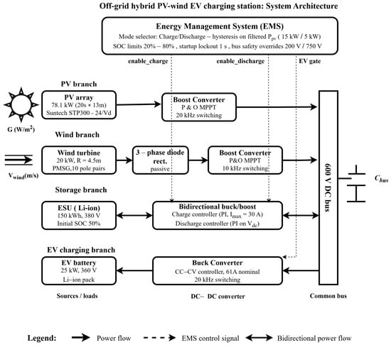
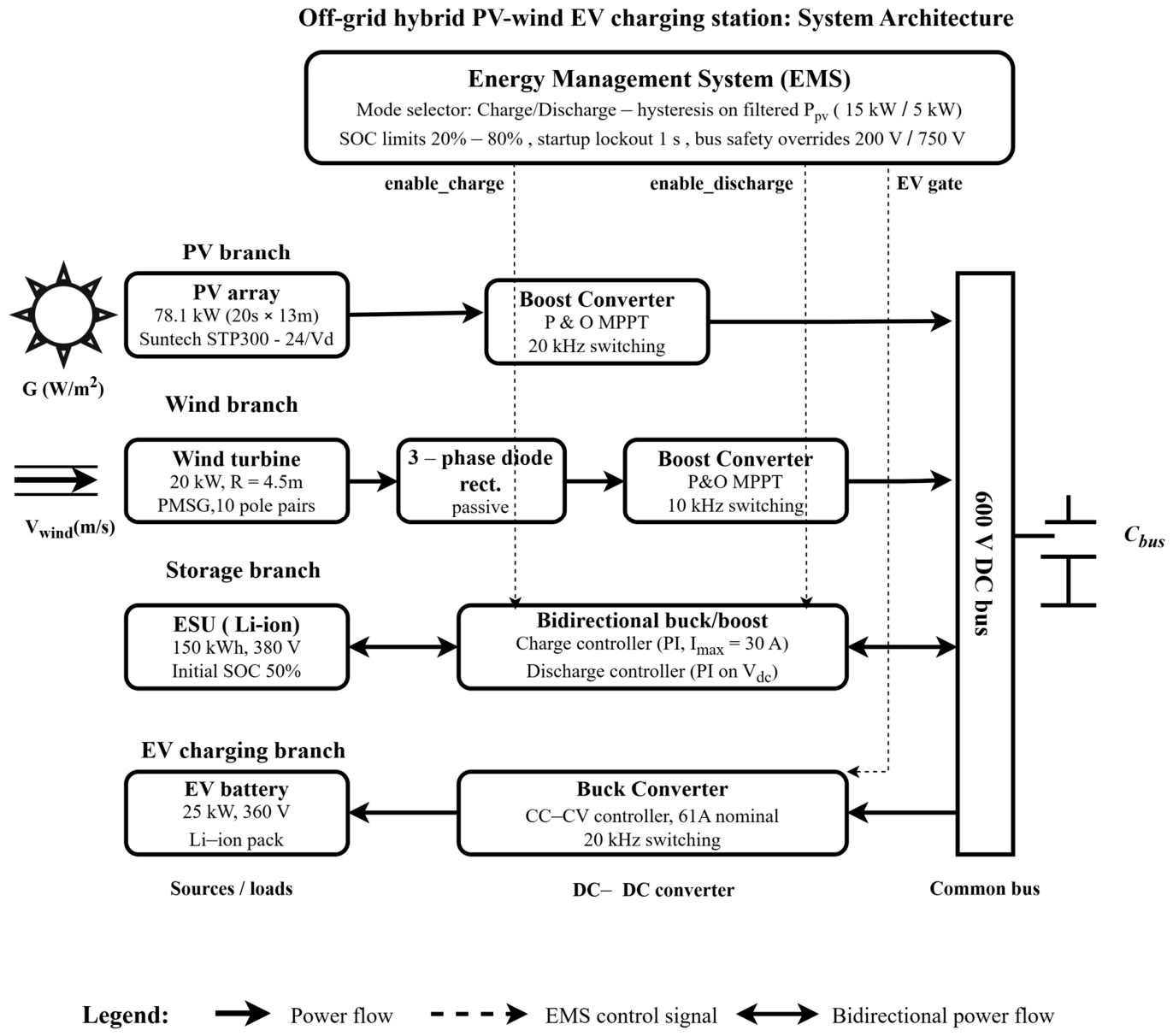
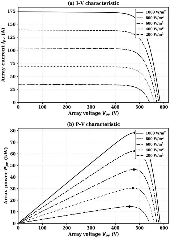
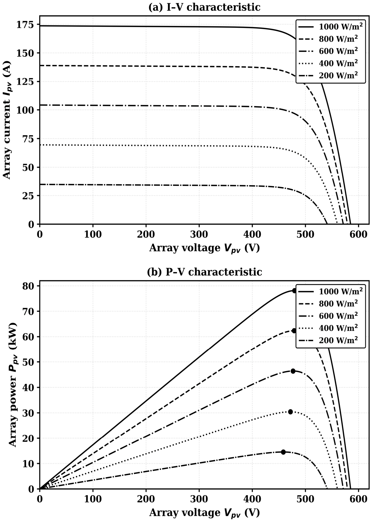
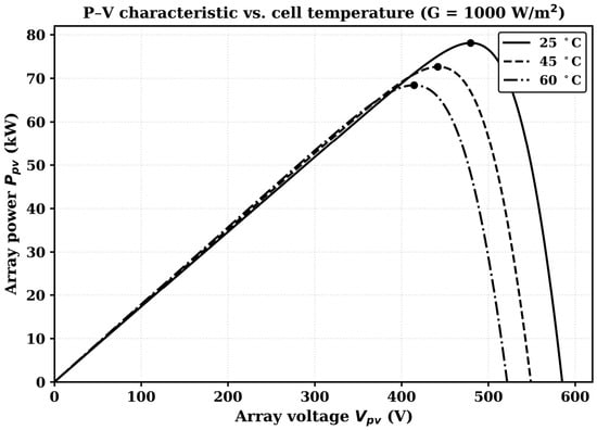
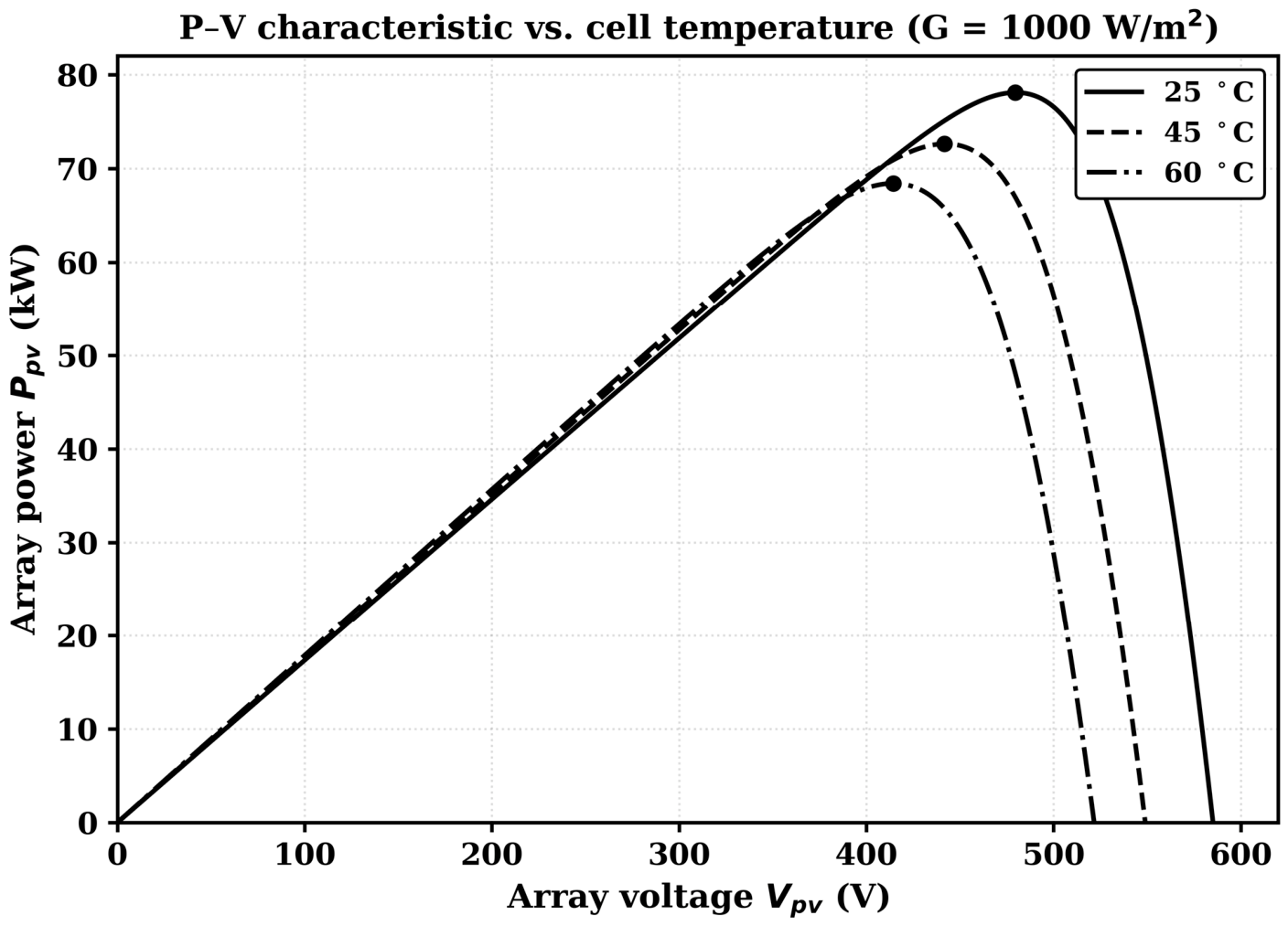
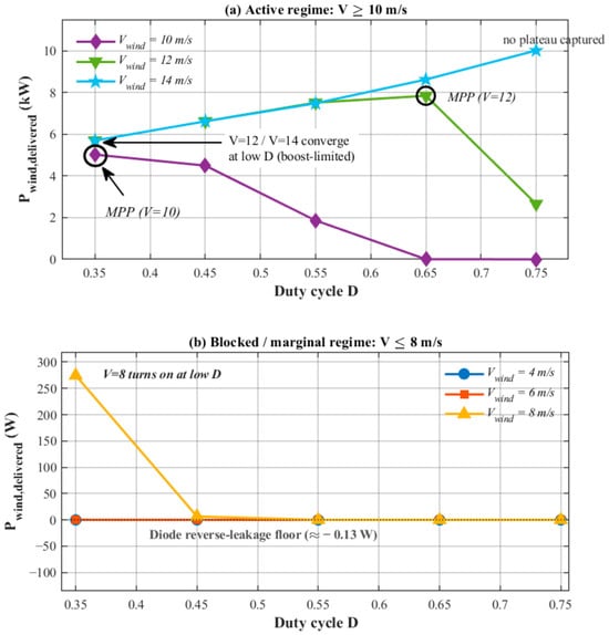
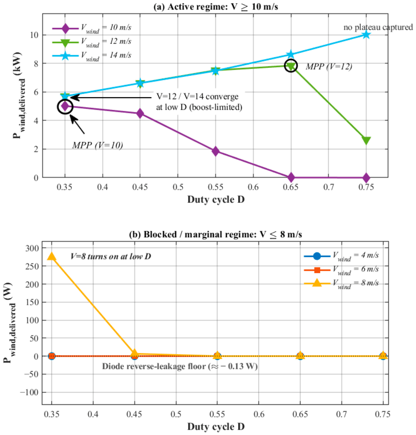
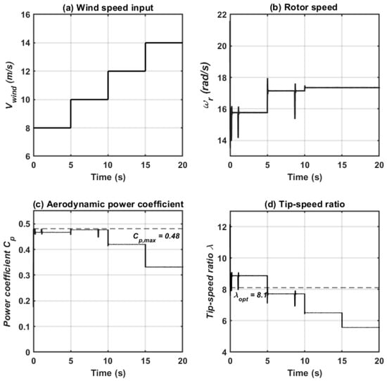
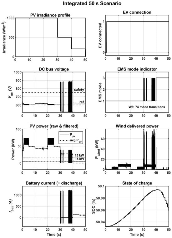
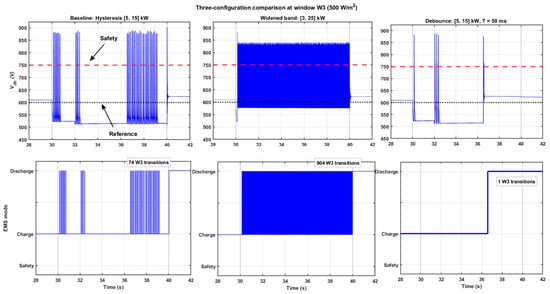
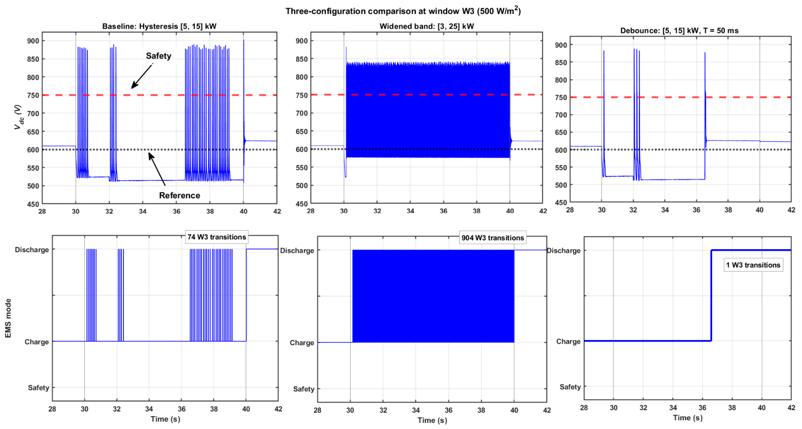

Disclaimer/Publisher’s Note: The statements, opinions and data contained in all publications are solely those of the individual author(s) and contributor(s) and not of MDPI and/or the editor(s). MDPI and/or the editor(s) disclaim responsibility for any injury to people or property resulting from any ideas, methods, instructions or products referred to in the content. |
© 2026 by the authors. Licensee MDPI, Basel, Switzerland. This article is an open access article distributed under the terms and conditions of the Creative Commons Attribution (CC BY) license.