Data-Driven Distributionally Robust Economic Dispatch of Offshore Engineering Microgrids: Multi-Functional Battery Coordination, Life-Cycle Cost Awareness, and Dual Time-Scale Optimization

Abstract

Offshore engineering microgrids integrate renewable generation, energy storage, and large marine test loads. Frequent start-stop transients of test loads, strong wind/PV fluctuations, and saline–humid conditions accelerate equipment aging and threaten power quality, while conventional dispatch neglects battery degradation, converter stress, and test-load energy recovery. This paper develops a data-driven distributionally robust economic dispatch method combining: (i) a priority-based dynamically weighted multi-functional battery coordination model unifying test-load surge suppression, renewable smoothing, and price arbitrage, with its coordinated reference embedded as a tracking constraint with an explicit two-level reserved margin; (ii) a two-stage Wasserstein distributionally robust optimization with adaptive ambiguity radii on standardized forecast errors and an improved column-and-constraint generation algorithm covering the full vertex set of the standardized uncertainty box; and (iii) a life-cycle-cost-aware objective with linearized battery degradation and converter power-variation stress under a dual time-scale (1 h day-ahead/15 min intraday) framework. Case studies on grid-connected and islanded offshore engineering microgrids show that multi-functional coordination lowers the post-storage maximum load ramp rate from 23.57 to 19.31 kW/min (−18.1%) and its standard deviation from 6.25 to 5.79 kW/min (−7.3%) at an operating-cost increase of 126.4 CNY/day, while reducing downstream renewable power fluctuation by 41.0% and recovering 102.0 kWh/day of test-load regenerative energy. The distributionally robust schedule attains a first-stage cost of 9492.5 CNY and, over 1000 independent realizations, reduces the out-of-sample mean cost from 9656.1 CNY (deterministic) to 9397.3 CNY and the 95% conditional value at risk (CVaR95) from 9940.5 to 9552.1 CNY, versus 10,698.3 CNY for a box-robust schedule with equivalent 95% coverage. The life-cycle-cost-aware dispatch reduces equivalent battery capacity fade by 37.1% and converter power-variation stress by 32.5% at +1.76% operating cost, while maintaining energy-based supply reliability at 99.79–100%. When the four mechanisms operate simultaneously, the maximum post-storage ramp is 19.31 kW/min against 23.57 kW/min for the unintegrated baseline (−18.1%), and removing the distributionally robust layer from the integrated schedule raises the out-of-sample CVaR95 of the recourse cost from 68.8 to 609.2 CNY/day. All optimization results are reproduced by two independent MILP solvers, with objectives agreeing within 2 × 10⁻⁹.

1. Introduction

Offshore engineering activities, including offshore platform construction, island development, marine engineering parks, and offshore wind-power bases, have expanded rapidly along with the growth of the marine economy [1,2,3]. Marine engineering parks host numerous high-capacity electrical devices, such as gantry cranes, welding machines, and metal cold-working machinery, and the test facilities at these parks for large generator sets and propulsion systems start and stop frequently with abrupt power impacts [4]. The resulting microgrids differ from onshore systems in several respects. Offshore wind, perturbed by turbulence and sea states, fluctuates more strongly, and PV output suffers from salt-fog shading. Marine test loads impose sharp load ramps that threaten power quality and even system security. A considerable portion of the electrical energy in load start-stop transients is dissipated, leaving an energy-recovery potential unexploited. Power-electronic converters are densely integrated and operate under saline–humid conditions that accelerate aging, and the batteries undergo frequent deep cycles, so that their degradation cost materially affects the true operating economy [5,6].

Microgrids have been widely recognized as an effective vehicle for integrating distributed renewable generation, energy storage, and controllable loads [5,7], and energy management systems (EMSs) play a central role in their economic operation [6,8]. Stochastic programming explicitly models the probability distribution of the uncertain parameters and has been applied to microgrid scheduling with intermittent renewables [9], but its performance degrades when the assumed distribution deviates from the true one. Robust optimization immunizes the schedule against the worst case within a deterministic uncertainty set [10,11] and is typically solved by column-and-constraint generation (C&CG) algorithms [12], yet it is often criticized for over-conservatism because it discards distributional information. Distributionally robust optimization (DRO) occupies the middle ground: it assumes that the true distribution lies within an ambiguity set constructed from data and optimizes the worst-case expectation over that set [13,14].

Among the available ambiguity sets, the Wasserstein-metric ball centered at the empirical distribution has received particular attention because it offers finite-sample performance guarantees and admits tractable reformulations [14,15]. Wasserstein DRO has been applied to power-system reserve co-optimization [13], frequency-constrained microgrid scheduling [16], islanded multi-microgrid design and operation [17], and two-stage islanded microgrid scheduling [18]. Two-stage day-ahead models for islanded microgrids that account for source-load uncertainties and demand response [19], and day-ahead microgrid models based on distributed robust optimization [20], have also been developed in the Chinese literature. Nevertheless, most existing DRO-based dispatch models target conventional onshore microgrids and rarely address the features that distinguish offshore engineering microgrids, namely the energy-recovery potential of frequently starting/stopping test loads, the multi-functional coordination of a single finite-capacity battery, and the joint life-cycle costing of batteries and power-electronic converters.

A storage unit in a microgrid must typically provide several services at once, such as peak shaving, renewable smoothing, voltage support, and frequency regulation [8,21,22]. Early studies assigned a single function to the battery energy storage system (BESS) or coordinated multiple functions heuristically: battery-based ramp-rate control of wind farms has been studied with hybrid sizing and control methods [23], and the joint optimization of peak shaving and frequency regulation has been shown to yield superlinear gains [22]. However, the conflict among surge suppression, fluctuation smoothing, and energy arbitrage under a finite power rating and state-of-charge (SOC) limits has not been systematically resolved for offshore engineering microgrids, where test-load surges and renewable fluctuations often coincide in time.

Battery degradation is likewise a first-order economic factor in storage scheduling. Semi-empirical degradation models based on cycle throughput and stress factors have been embedded into scheduling frameworks for cell life assessment [24], and degradation-aware scheduling has been shown to reduce the total cost of ownership [22]. Power-electronic converters, whose reliability is strongly affected by thermal cycling under power variations [25,26], are usually idealized in dispatch models, so their lifetime consumption is rarely charged to the schedule. In offshore grids, where the converter interfacing the battery experiences frequent and rapid power swings, this neglect biases the schedule toward aggressive battery cycling.

On the time-scale side, hierarchical scheduling with a day-ahead layer at 1 h resolution and an intraday layer at 15 or 5 min resolution is widely adopted to reconcile unit commitment with fine-grained re-dispatch [27]. Such dual time-scale structures suit microgrids with strong intra-hour fluctuations, yet their combination with DRO and life-cycle costing has rarely been studied for offshore engineering microgrids.

Motivated by these gaps, this paper develops a Wasserstein-DRO-based economic dispatch framework for offshore engineering microgrids. The positioning of this work relative to closely related studies is compared in Table 1, and the main contributions are summarized as follows: (i) the marine test-load model is coupled to the storage controller through an explicit regenerative-energy channel, so that the energy-recovery potential of the test loads becomes a decision variable and the resulting schedule is charged for the converter stress it induces; (ii) multi-functional battery coordination is formulated as a constrained allocation on the weight simplex with an explicit two-level arbitration rule whose solution is provably no worse than that of the uncoordinated problem and whose residual ramp limitation is attributed to the converter rating rather than to the coordination logic; (iii) the Wasserstein ambiguity set is defined on standardized forecast errors and its radius is calibrated on an independent validation set, while the worst-case sub-problem is solved over the complete vertex set of the standardized uncertainty box; and (iv) battery and converter aging are costed jointly inside a receding-horizon dual time-scale schedule, with the scope and the limits of the linearized aging surrogates quantified against higher-fidelity models.

Table 1. Positioning of this work with respect to closely related studies.

Study Group	Offshore Test-Load Modeling	Test-Load Energy Recovery	Multi-Functional BESS with Explicit Conflict Arbitration	Converter Stress Costing	Standardized Ambiguity Set with Validation-Set Radius	Dual Time Scale with Receding Horizon
[8,22,23]	N	N	P	N	N	P
[13,16,17,18]	N	N	N	N	P	P
[24]	N	N	N	N	N	P
[25,26]	N	N	N	Y	N	N
[4]	P	N	N	N	N	N
This work	Y	Y	Y	Y	Y	Y

Note: Y = addressed, P = partially addressed, N = not addressed.

The remainder of this paper is organized as follows. Section 2 describes the offshore engineering microgrid system and the base economic dispatch model. Section 3 presents the multi-functional coordination model of the battery. Section 4 formulates the Wasserstein distributionally robust optimization framework and the improved C&CG solution algorithm. Section 5 develops the life-cycle-cost-aware objective and the dual time-scale coordination scheme. Section 6 reports the case studies, and Section 7 concludes the paper.

2. Materials and Methods

2.1. Offshore Engineering Microgrid Architecture

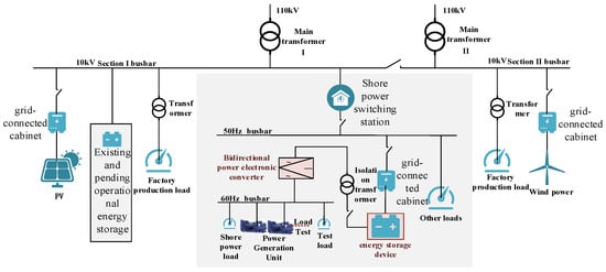
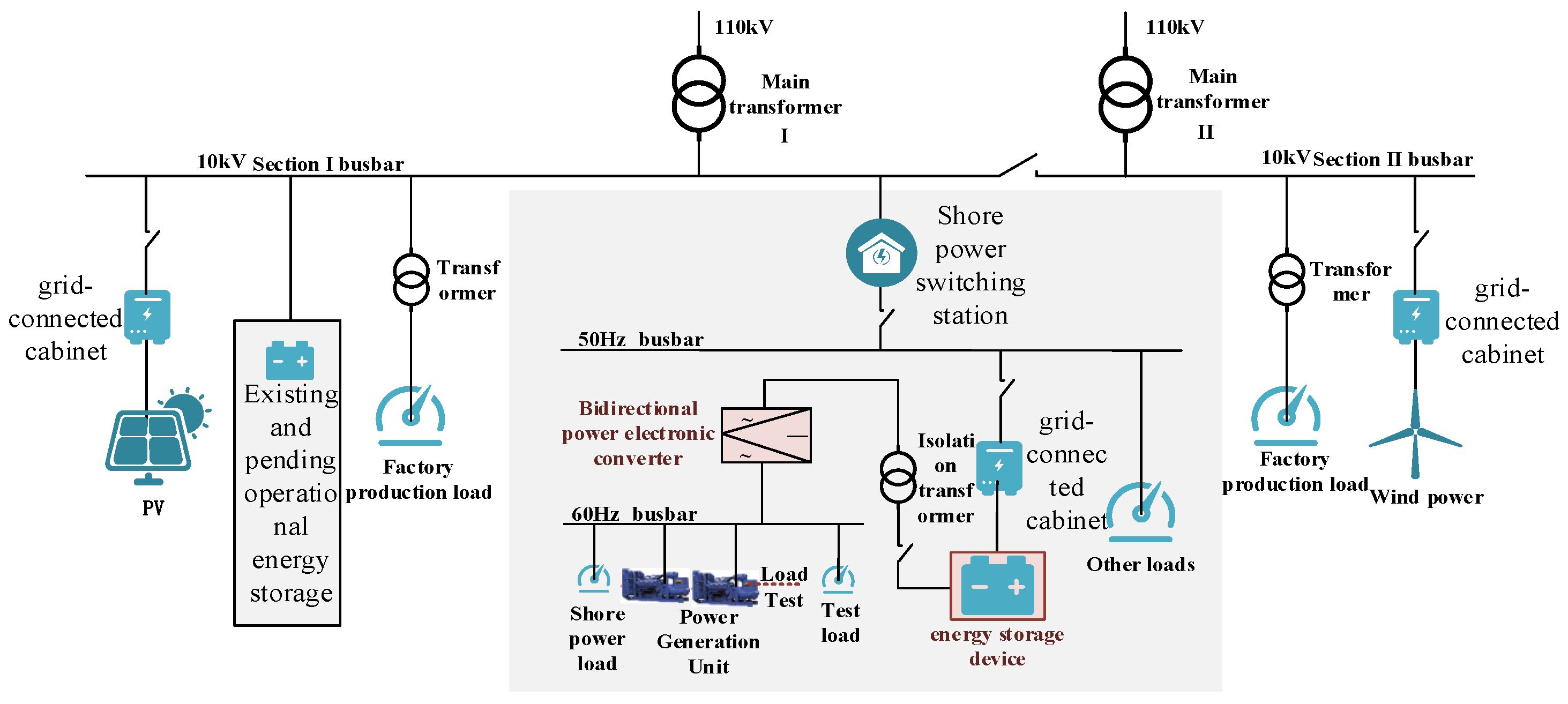
The offshore engineering microgrid considered in this study is illustrated in Figure 1. It integrates wind turbines, PV arrays, diesel generators, a battery energy storage system (BESS) interfaced through a bidirectional power-electronic converter, and the marine test loads (e.g., generator load-test banks and propulsion test rigs), and general service loads. The microgrid can operate in the grid-connected mode, where a bidirectional interface with the main grid (typically at 10 kV/50 Hz) enables purchasing and selling, or in the islanded mode, where diesel generators and the BESS must balance the load. In the grid-connected mode, the large bidirectional converter can also perform energy recovery during generator load tests by converting the non-standard-frequency power (e.g., 11 kV/60 Hz) produced by the tested generator into standard-frequency power and storing the recovered energy in the battery, thereby partially replacing the load banks and improving energy efficiency.

Figure 1. Architecture of the offshore engineering microgrid considered in this study.

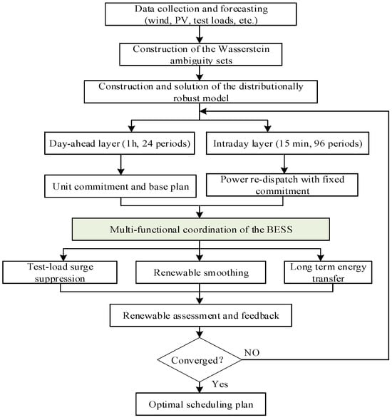
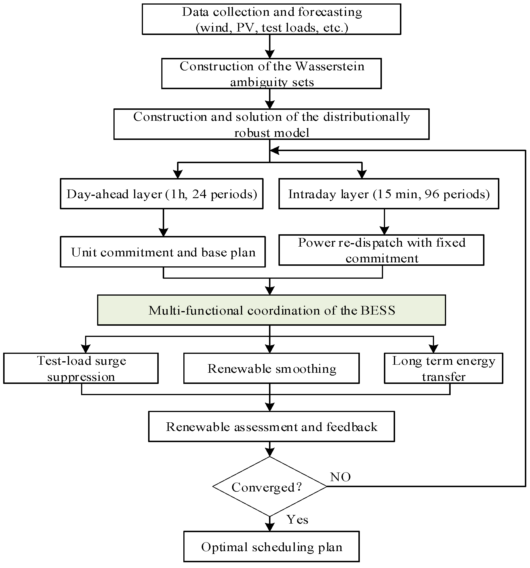
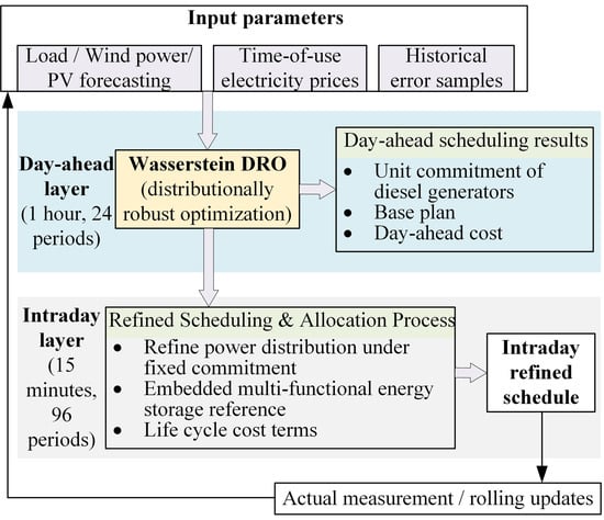
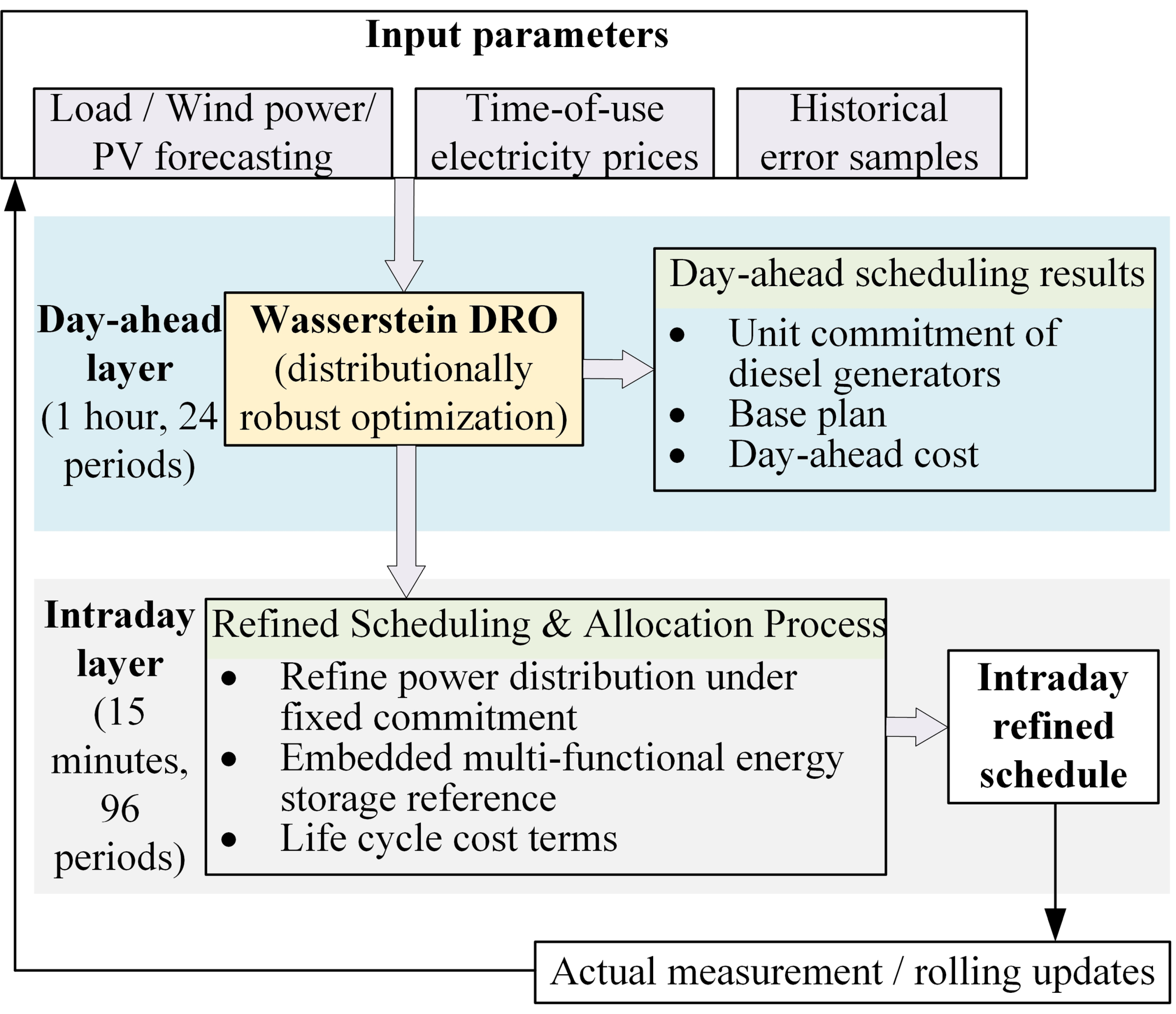
The overall framework of the proposed method is shown in Figure 2, and the dual time-scale coordination is illustrated in Figure 3. The day-ahead layer (1 h resolution, 24 h horizon) minimizes the total cost to determine the unit commitment and the base operating plan; the intraday layer (15 min resolution, 96 periods) refines the power allocation under the fixed day-ahead commitment, embedding the multi-functional battery reference and the life-cycle-cost terms. Uncertainties of wind power, PV power, and test loads are handled by the Wasserstein distributionally robust optimization in both layers.

Figure 2. Overall architecture and flowchart of the proposed economic dispatch method.

Figure 3. Framework of the dual time-scale coordination between the day-ahead (1 h) and intraday (15 min) layers.

2.2. Base Economic Dispatch Model

Let T = {1, 2, …, N} denote the set of time intervals with time step Δt (h). In the grid-connected mode, the power balance is given:

$$P_w\left(t\right)+P_{\mathit{pv}}\left(t\right)+\sum _i{P}_{\mathit{dg},i}\left(t\right)+P_{\mathit{dis}}\left(t\right)+P_{\mathit{buy}}\left(t\right)=P_L\left(t\right)+P_{\mathit{cha}}\left(t\right)+P_{\mathit{sell}}\left(t\right)$$

(1)

where P_w(t), P_pv(t), P_dg,i(t), P_dis(t), P_cha(t), P_buy(t), P_sell(t), and P_L(t) denote the wind power, PV power, diesel output of unit i, battery discharging power, battery charging power, grid purchasing power, grid selling power, and load at interval t, respectively. In the islanded mode, the grid-interaction terms are replaced by the load-shedding variable P_shed(t):

$$P_w\left(t\right)+P_{\mathit{pv}}\left(t\right)+\sum _i{P}_{\mathit{dg},i}\left(t\right)+P_{\mathit{dis}}\left(t\right)+P_{\mathit{shed}}\left(t\right)=P_L\left(t\right)+P_{\mathit{cha}}\left(t\right)$$

(2)

The battery net power and the SOC dynamics are

P_bat(t) = P_dis(t) − P_cha(t)

(3)

$$\mathit{SOC}(t+1)=\mathit{SOC}\left(t\right)+{\displaystyle \frac{\left({\eta }_{\mathit{ch}}{P}_{\mathit{cha}}\right(t)-\frac{P_{\mathit{dis}}\left(t\right)}{{\eta }_{\mathit{dis}}})\Delta t}{E_B}}$$

(4)

where η_ch and η_dis are the charging and discharging efficiencies, E_B is the battery rated capacity, and the initial SOC is SOC(1) = SOC₀. The charging and discharging are mutually exclusive, i.e., u_cha(t) + u_dis(t) ≤ 1 with P_cha(t) ≤ P_cs…u_cha(t) and P_dis(t) ≤ P_cs · u_dis(t), where P_cs is the converter power rating. The SOC is bounded by [SOC_min, SOC_max] and the terminal SOC is kept close to its initial value, i.e., |SOC(N+1) − SOC₀| ≤ 0.05.

Each diesel generator is subject to the minimum technical output, capacity, and start-up constraints:

$$P_{\mathit{dg}}^{\mathit{min}}·u_{\mathit{dg},i}\left(t\right)\le P_{\mathit{dg},i}\left(t\right)\le P_{\mathit{dg}}^{\mathit{max}}·u_{\mathit{dg},i}\left(t\right)$$

(5)

v_dg,i(t) ≥ u_dg,i(t) − u_dg,i(t − 1), v_dg,i(t) ≤ u_dg,i(t), v_dg,i(t) ≤ 1 − u_dg,i(t − 1)

(6)

where u_dg,i(t) ∈ {0,1} is the commitment state and v_dg,i(t) ∈ {0,1} indicates the start-up event. In the grid-connected mode, the grid-interaction power is bounded by the interface capacity P^GRID and the purchase/sale states are mutually exclusive through big-M constraints. Renewable generation is curtailable, i.e., 0 ≤ P_w(t) ≤ P_w^f(t) and 0 ≤ P_pv(t) ≤ P_pv^f(t), where the superscript f denotes the forecast value. Load shedding is bounded by 0 ≤ P_shed(t) ≤ P_L(t).

3. Multi-Functional Coordination Model of the Battery Energy Storage System

Under a finite power rating and energy capacity, a single BESS cannot simultaneously deliver full surge suppression, complete fluctuation smoothing, and optimal arbitrage. This section proposes a coordination model that decomposes the battery power demand into three functional components and allocates the limited power capacity among them according to a priority mechanism that adapts to the system operating state.

3.1. Test-Load Surge Suppression

The marine test loads start and stop frequently, producing abrupt power ramps that may exceed the tolerable rate of the system. The surge-suppression component detects the load change rate and compensates for the part that exceeds a threshold R_th:

$$P_{\mathit{ld}}\left(t\right)=\max (-P_{\mathit{cs}},\min (P_{\mathit{cs}},k_l·\max (0,{\displaystyle \frac{|\Delta P_L(t\left)\right|}{\Delta t}}-R_{\mathit{th}})·\mathrm{sgn}(\Delta P_L(t\left)\right)\left)\right)$$

(7)

where ΔP_L(t) = P_L(t) − P_L(t−1) is the load variation, k_l is the suppression gain, and the clipping to [−P_cs, P_cs] ensures that the battery discharges (positive) when the load rises and charges when the load drops, so that the net-load ramp seen by the grid and the diesel generators is confined within the threshold.

3.2. Renewable-Energy Fluctuation Smoothing

The smoothing component counteracts the weighted forecast errors of wind and PV generation:

P_re(t) = −(w_w · ΔP_w(t) + w_pv · ΔP_pv(t)), where w_w + w_pv = 1

(8)

where ΔP_w(t) = P_w^a(t) − P_w^f(t) and ΔP_pv(t) = P_pv^a(t) − P_pv^f(t) are the wind and PV forecast errors (the superscript a denotes the actual value), and w_w, w_pv are the weighting coefficients. The negative sign makes the battery absorb surplus renewable power (charge) when the actual generation exceeds the forecast, and release power when it falls short.

3.3. Long-Term Energy Transfer

The energy-transfer component shifts energy across time according to the time-of-use (TOU) price signal and restores the SOC toward its mid-range value:

$$P_{\mathit{tr}}\left(t\right)=k_{\mathit{tr}}·{\displaystyle \frac{C_b\left(t\right)-{\overline{C}}_b}{C_b^{\mathit{max}}-C_b^{\mathit{min}}}}·P_{\mathit{cs}}+P_{\mathit{soc}}\left(t\right)$$

(9)

$$P_{\mathit{soc}}\left(t\right)=-k_{\mathit{soc}}·{\displaystyle \frac{\mathit{SO}{C}_{\mathit{mid}}-S\widehat{O}C\left(t\right)}{\mathit{SO}{C}^{\mathit{max}}-\mathit{SO}{C}^{\mathit{min}}}}·P_{\mathit{cs}}$$

(10)

where C_b(t) is the purchase price, ${\stackrel{-}{C}}_b$ is the average price over the horizon, C_b^max and C_b^min are the maximum and minimum prices, k_tr is the arbitrage gain, $S\widehat{O}C\left(t\right)$ is the open-loop estimated SOC based on the arbitrage power integration, SOC_mid = (SOC_min + SOC_max)/2, and k_soc is the SOC-restoration gain. The component is clipped to [−0.5P_cs, 0.5P_cs] to reserve capacity for the other functions.

3.4. Priority-Based Dynamic Weighting and Power Coordination Allocation

Because the three components may conflict (e.g., a load surge and a renewable fluctuation occurring simultaneously with an arbitrage signal), a priority mechanism dynamically adjusts their weights. When the load variation exceeds the surge threshold, the system is regarded as being in an emergency state and the surge-suppression weight is raised; otherwise, the normal weights apply:

w_normal = [0.30, 0.40, 0.30],      w_emerg = [0.80, 0.10, 0.10]

(11)

where the three entries correspond to [surge suppression, fluctuation smoothing, energy transfer]. The effective weight at interval t is w(t) = w_normal when the per-interval load step satisfies |ΔP_L(t)| ≤ R_th, and w(t) = w_emerg otherwise, with R_th = 400 kW/h, i.e., 100 kW per 15 min interval or 6.67 kW/min, as listed in Table 2 and Table 3, and with the adopted weight vectors w_normal = [0.30, 0.40, 0.30] and w_emerg = [0.60, 0.20, 0.20]. The weights are normalized, and the coordinated battery reference is obtained as the weighted sum clipped to the converter rating:

Table 2. Quantified characteristics of the offshore engineering microgrid test system.

Characteristic	Grid-Connected	Islanded
General service load min/mean/max (kW)	42/336/836	55/435/1086
Test-load events per day	6 (3 power-up, 3 trip)	6
Surge magnitudes (kW)	+200, −200, −150, +150, +180, −180	same
Surge duration (h)	0.50 (power-up), instantaneous (trip), 0.50/0.75	same
Surge frequency	3 events in 07:30–11:45, 2 in 16:00–17:00, 1 at 08:15	same
Largest single-interval load step (kW)	334	388
Regenerative intervals/recoverable energy	3 per day/102.0 kWh per day	3 per day
Wind installed/forecast (kW)	240/79–211	240/79–211
PV installed/forecast (kW)	260/0–237	260/0–237
BESS energy/power	500 kWh/200 kW	250 kWh/250 kW
Bidirectional converter	200 kW, efficiency > 98%	250 kW, efficiency > 98%
Grid interconnection	400 kW, 10 kV/50 Hz	not applicable
Diesel units	1 × 500 kW back-up	3 × 500 kW, Pmin = 150 kW
Reserve requirement: surge/uncertainty (kW)	not binding	128/175
Reserve requirement: energy (kWh)	not binding	118
Reserve available from the BESS (kW/kWh)	200/147	240/147
Controller ramp threshold Rth (kW/h)	400	400
Coordination margin normal/emergency (p.u. of Pcs)	0.35/0.35	0.35/0.35
Slack penalty normal/emergency (CNY per kWh)	0.20/2.00	0.20/2.00
DRO training/validation/test samples	200/700/1000	200/700/1000
Ambiguity radius selected on validation set	ε· = 0.25	0.25
Solver	intlinprog, 1 × 10−4 gap, verified with CPLEX	same

Table 3. Main parameters of the offshore engineering microgrid cases.

Parameter	Symbol	Grid-Connected	Islanded
Load range	PL	42–836 kW	55–1086 kW
Wind/PV forecast	Pwf, Ppvf	240 kW/260 kW installed; 79–211/0–237 kW forecast	240 kW/260 kW installed; 79–211/0–237 kW forecast
Diesel generators	Pdgmax, Pdgmin	N/A	3 × 500/150 kW
Battery capacity/power	EB, Pcs	500 kWh/200 kW	250 kWh/250 kW
SOC limits/initial	SOCmin, SOCmax, SOC0	0.15/0.90/0.50	0.15/0.90/0.60
Charging/discharging efficiency	ηch, ηdis	0.95/0.95	0.95/0.95
Grid interface capacity	PGRID	400 kW	N/A
Diesel fuel/start-up cost	cdg, csu	N/A	2.0 CNY/kWh, 300 CNY/start
TOU purchase price	Cb	1.6–3.6 CNY/kWh	reference
TOU sale price	Cs	0.6–1.4 CNY/kWh	reference
Load-shedding/curtailment penalty	csh, ccu	10/0.5 CNY/kWh	10/0.5 CNY/kWh
Battery investment/cycles	Cinvbat, Ncyc	2000 CNY/kWh, 4500	4000 CNY/kWh, 4500
Converter investment/lifetime	Cinvconv, Lconv	2500 CNY/kW, 1 × 105 h	2500 CNY/kW, 1 × 105 h
Surge threshold/suppression gain	Rth, kl	Rth = 400 kW/h, kl = 1.0	Rth = 400 kW/h, kl = 1.0
Coordination margin/slack penalty	δref, cslack	δref 0.35/δemerg 0.35; cslack 0.20/2.00 CNY/kWh	δref 0.35/δemerg 0.35; cslack 0.20/2.00 CNY/kWh
DRO samples/radius scale	Ns, εscale	ε· = 0.25, 200 (train)/700 (validation)/1000 (test);	ε· = 0.25, 200 (train)/700 (validation)/1000 (test);
C&CG gap tolerance/max iterations	gaptol, itermax	1 × 10−4 C&CG gap, 1 × 10−4 MILP gap, max 5 iterations	1 × 10−4 C&CG gap, 1 × 10−4 MILP gap, max 5 iterations

3.5. Priority-Based Arbitration and Reserved Margin

The three requests are combined through weights constrained to the probability simplex, w_i(t) ≥ 0 and ${\sum }_i{w}_i\left(t\right)=1$, so that the reference is a convex combination of the three functional requests and no request can be amplified beyond its own magnitude. The priority switch is explicit: w(t) = w_normal when |dP_L(t)|/dt ≤ R_th and w(t) = w_emerg otherwise, with w_emerg,1 > w_normal,1 so that surge suppression dominates in the emergency state. The coordinated reference is $P_{\mathit{ref}}\left(t\right)=\mathit{clip}\left({\sum }_i{w}_i\right(t\left)P_i\right(t),{-P}_{\mathit{cs}},P_{\mathit{cs}})$.

The reference enters the dispatch as a band constraint with a state-dependent width and a non-negative slack, |P_bat(t) − P_ref(t)| ≤ δ(t) + s(t), where δ(t) = δ_ref P_cs with slack penalty c_slack in the normal state and δ(t) = δ_emerg P_cs with penalty c_slack,emerg = 10 c_slack in the emergency state. This two-level hierarchy is the mathematical form of the conflict arbitration: in the normal state the economics retain full freedom within a 70 kW band, whereas in the emergency state the surge request is enforced almost exactly and can only be relaxed, at high cost, when the power or SOC limits make it physically infeasible.

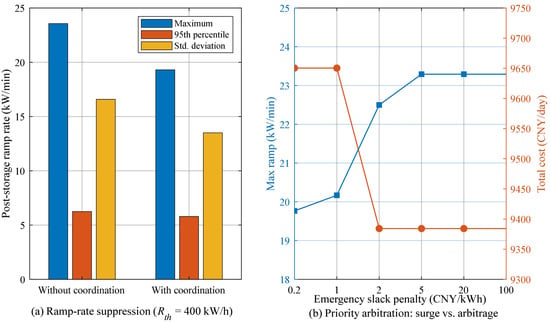
Because δ(t) ≥ 0 and s(t) is unbounded above, the feasible set of the coordinated dispatch is a superset of the uncoordinated feasible set; consequently, the coordinated optimum can never be worse than the uncoordinated optimum before the slack penalty is accounted for, which guarantees that the coordination layer can never render the dispatch infeasible. The residual post-coordination ramp is limited by the converter rating rather than by the arbitration rule: increasing the emergency slack penalty beyond 2 CNY/kWh does not reduce the ramp further.

3.6. Power and Energy Reserve Margins

Two quantities that were conflated in the first version are now defined separately. The tracking bandwidth δ(t) is a power relaxation that preserves the economic freedom of the dispatch and is not a physical reserve. The reserve is defined independently as the power and energy capability that must remain uncommitted, $R_p^{\mathit{up}}\left(t\right)=P_{\mathit{cs}}-P_{\mathit{dis}}\left(t\right)$, $R_p^{\mathit{dn}}\left(t\right)=P_{\mathit{cs}}-P_{\mathit{cha}}\left(t\right)$, $E_r^{\mathit{up}}\left(t\right)={(\mathit{SOC}}_{\mathit{max}}-\mathit{SOC}\left(t\right))E_B$ and $E_r^{\mathit{dn}}\left(t\right)=\left(\mathit{SOC}\right(t)-{\mathit{SOC}}_{\mathit{min}})E_B$. The requirement is derived from data: the largest test-load surge requires 128 kW, whereas the 95th percentile of the historical net forecast error requires 175 kW, so the uncertainty requirement governs; 118 kWh of energy reserve correspond to four hours at that power. The islanded case is feasible with respect to both (240 kW and 147 kWh available), but the requirement consumes up to 73% of the converter rating.

P_ref(t) = w₁(t) · P_ld(t) + w₂(t) · P_re(t) + w₃(t) · P_tr(t)

(12)

The reference is embedded into the dispatch model as a tracking constraint with a reserved coordination margin δ(t) = δ_ref…P_cs and a non-negative slack s(t):

|P_bat(t) − P_ref(t)|≤δ(t) + s(t)

(13)

The margin δ(t) preserves the freedom of the economic optimization, and the slack s(t), penalized with a small coefficient c_slack in the objective, guarantees feasibility under extreme conditions. In this way, the multi-functional coordination guides the battery toward surge suppression, fluctuation smoothing, and arbitrage without strictly forcing the schedule, so that the finite storage capacity is shared among the conflicting functions while the economic optimum is preserved to the greatest extent.

4. Wasserstein Distributionally Robust Optimization Framework

4.1. Uncertainty Modeling of Wind, PV, and Test Loads

The uncertain parameters are the forecast errors of wind power ξ_w, PV power ξ_pv, and load ξ_L. Historical samples are generated from the forecast curves with output-dependent standard deviations (10% for wind, 15% for PV, and 5% plus a constant for the load), and the cross-source correlation is imposed through the Cholesky decomposition of a correlation matrix with coefficients R_w,pv = −0.25, R_w,L = 0.15, and R_pv,L = 0.10, reflecting the negative wind-PV correlation and the mild positive correlation of the load with renewable generation. Let P^N denote the empirical distribution of the N_s samples ξⁱ = (ξ_wⁱ, ξ_pvⁱ, ξ_Lⁱ) ∈ Ξ, i.e., the equally weighted mixture of the Dirac measures concentrated at the samples. The corresponding ambiguity set is constructed in the next subsection. The standardized error of source j at interval t is defined as ξ_j(t)/σ_j(t), where σ_j(t) is the mean absolute deviation of its historical forecast errors, so that the three sources are expressed in units of their own typical error; the support of the ambiguity set is the standardized box Ξ = {ξ: |ξ_j(t)| ≤ 1 for j ∈ {w, p_v, L} and all t}. The empirical distribution, this standardized support, the L₁ ground metric and the dimensionless radius of Section 4.2 are the objects linked by the derivation of Section 4.2, Section 4.3 and Section 4.4.

4.2. Wasserstein Ambiguity Set

The Wasserstein distance between two distributions P₁ and P₂ on the support Ξ is defined as follows:

$$d_W(P_1,P_2)=\underset{\Pi }{\inf }{\int }_{\Xi \times \Xi }\Vert {\xi }_1-{\xi }_2\Vert \Pi (d{\xi }_1,d{\xi }_2)$$

(14)

where Π ranges over all joint distributions with marginals P₁ and P₂ and ||·|| is a norm on the uncertainty space. The Wasserstein ambiguity set is the ball of radius ε centered at the empirical distribution:

$$D=\{P\in M(\Xi ):d_W(P,{\widehat{P}}_N)\le \epsilon \}$$

(15)

where M(Ξ) is the set of all probability distributions supported on Ξ. The ball radius ε is adapted to the per-slot prediction-error statistics:

ε(t) = ε_scale · σ_typ(t) · (1 + α_adapt · κ_L(t))

(16)

where σ_typ(t) = σ_w(t) + σ_pv(t) + σ_L(t) is the sum of the mean absolute deviations of the wind, PV, and load forecast errors at interval t. Let σ_j(t) denote the mean absolute deviation of the historical forecast errors of source j at slot t and define the standardized error vector by ξ_j(t)/σ_j(t); the ground metric of the Wasserstein distance is the standardized L₁ metric, so that the radius is dimensionless and directly comparable with the half-width of a Gaussian-quantile box. The adaptive radius is ε(t) = ε_scale(1 + α_adapt κ_L(t)) with κ_L(t) = σ_L(t)/P_L(t), and the physical radius of source j at slot t is ε_j(t) = ε(t)σ_j(t). The radius therefore adapts to the local forecast quality and to the relative uncertainty of the load, not to the sample size or to a rolling window. Statistically, the finite-sample result of Esfahani and Kuhn guarantees that the true distribution lies inside the ball with probability at least 1 − β whenever the radius exceeds a quantity of order $\sqrt{\mathit{log}(1/\beta )/N_s}$; with N_s = 200 training samples this certifies a radius of the same order as the value selected on the validation set (ε = 0.25). When ε_scale = 0 the ambiguity set shrinks to the empirical distribution and the model degenerates to the deterministic one; when ε is enlarged to cover the full standardized box, the model approaches the traditional box-type robust optimization.

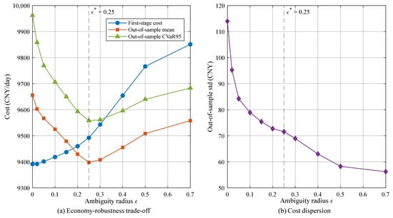
The radius is calibrated rather than inspected. Eleven candidate values of ε_scale ∈ {0, 0.02, 0.05, 0.10, 0.15, 0.20, 0.25, 0.30, 0.40, 0.50, 0.70} are evaluated on 700 validation realizations (seeds 202 and 555) with the criterion J(ε) = mean + one standard deviation of the validation cost, and ε* = 0.25 attains the interior minimum (9400.7 CNY, against 9662.2 CNY at ε = 0 and 9560.7 CNY at ε = 0.70). The 1000 test realizations (seed 7777) are used once, after the selection, and never enter J(ε).

4.3. Two-Stage Distributionally Robust Formulation

The day-ahead (first-stage) decisions x, including the diesel commitment and the base dispatch of all units, are made before the uncertainty is realized. The second-stage (recourse) decisions y (load shedding, renewable curtailment, battery power and SOC deviations, and grid-interaction deviations) are adjusted after the realization. The two-stage distributionally robust model is as follows:

$$\underset{x\in X}{\min }(c^{T}x+\underset{P\in D}{\max }{E}_P[Q(x,\xi )\left]\right)$$

(17)

$$Q(x,\xi )=\underset{y\in Y(x,\xi )}{\min }{q}^{T}y$$

(18)

where X is the first-stage feasible region, c is the first-stage cost vector, q is the recourse cost vector, Y(x,ξ) is the second-stage feasible region parameterized by (x,ξ), and E_P[·] denotes the expectation under the distribution P. The recourse cost penalizes load shedding (c_shed), renewable curtailment (c_curt), battery power deviations from the first-stage plan (c_essdev), SOC deviations (c_socdev), and grid-interaction deviations (c_gi)or diesel-output deviations (c_dd) in the islanded mode.

The inner supremum of (18) is taken over distributions rather than over realizations, and it therefore cannot be evaluated by enumerating forecast errors. For a finite support, a norm-based ground metric and an integrable recourse function it admits the dual representation (19), in which the inner supremum runs over the support Ξ and λ ≥ 0 is the multiplier associated with the radius constraint [14]. Equation (19) is the exact worst-case expectation of the ambiguity set (15); it is stated here because it defines the quantity that the algorithm of Section 4.4 approximates, and because it shows that the worst case is a distributional object rather than a single most-adverse error vector.

$$\underset{P\in D}{\sup }\hspace{0.17em}{\mathrm{E}}_P\left[Q\left(x,\xi \right)\right]=\underset{\lambda \ge 0}{\min }\left\{\mathit{\lambda \epsilon }+1/\mathrm{N}{\displaystyle \sum _{i=1}^N}\underset{\xi \in \mathsf{\Xi }}{\sup }\left[Q\left(x,\xi \right)-\lambda {‖\xi -{\xi }_i‖}_1\right]\right\}$$

(19)

Two consequences of (19) are used below. First, the worst-case expectation is bounded above by the support worst case, i.e., by the maximum of Q(x, ξ) over Ξ, because the expectation of a random variable cannot exceed its maximum; that maximum is computable, since Q(x, ·) is convex and piecewise linear in ξ and a convex function attains its maximum over a box at a vertex. Second, the empirical distribution belongs to the ball, so the worst-case expectation is bounded below by the sample-mean recourse cost. Equation (19) therefore brackets the quantity of interest between two computable ends, and the algorithm of Section 4.4 returns an inner approximation between them.

4.4. Improved Column-and-Constraint Generation Algorithm

The two-stage model is solved by an improved column-and-constraint generation (C&CG) algorithm. Let S denote the set of discovered scenarios. The master problem contains the first-stage decisions and one recourse block per discovered scenario, together with an auxiliary variable θ that upper-bounds the worst-case recourse cost:

minc^Tx + θ

(20)

subject to x ∈ X, θ ≥ 0, and for each s ∈ S,

θ ≥ q^Ty_s,       A_sx + By_s ≥ h_s

(21)

Given the first-stage solution x*, the sub-problem evaluates the recourse cost Q(x*, ξ) at nine candidate realizations: the sample center ξ = 0 and the eight sign patterns ξ_j(t) = s_j · ε_j(t) with s_j ∈ {−1, +1}, where ε_j(t) is the physical radius of source j at interval t defined in Section 4.2. The candidate set is therefore the vertex set of the standardized ε-box. Because Q(x*, ·) is the value function of a linear program whose right-hand side is affine in ξ, it is convex and piecewise linear in ξ, and a convex function attains its maximum over a box at a vertex; the sub-problem is therefore exact for the maximum of the recourse cost over that box, and it requires nine recourse evaluations instead of one per historical sample.

The status of the resulting value is stated explicitly, because it is easy to over-claim. The sub-problem maximizes the recourse cost over a subset of the support, so the value it returns, denoted Q_v(x), is a lower bound on the support worst case max Q(x, ξ) over Ξ and, through (19), an inner approximation of the worst-case expectation: it is not an exact evaluation of (19), and it is not a bound on individual realizations. The direction and the size of the approximation are quantified rather than asserted: a variant that searches all N_s = 200 training samples returns a value 2.1% higher than the nine-vertex variant on the same instance (9662.06 against 9459.93 CNY, Section 6.11), because the empirical samples lie farther from the centre than the vertices of the ε-box, and the support worst case closes the bracket from above. The paper therefore reports three distinct quantities and names them consistently: the vertex worst case Q_v (the return of the algorithm), the sample worst case Q_s (its tighter inner approximation) and the support worst case max Q over Ξ (the certified upper end).

The lower bound L_B is the master-problem objective and the upper bound U_B is the sum of the first-stage cost and the vertex worst-case recourse cost; the iteration stops when (U_B − L_B)/|L_B| ≤ 1 × 10⁻⁴. In the reported configuration the algorithm converges in two iterations and 18 recourse evaluations (Section 6.11). The recourse linear program is assembled in closed sparse form, which reduces its solution time by more than an order of magnitude relative to the general-purpose modeling layer without changing the optimum (relative difference below 1 × 10⁻¹⁵ in the verification runs). In the box-type robust mode the eight vertices of the calibrated box are pre-embedded as scenarios and the problem is solved in a single pass.

5. Life-Cycle-Cost-Aware Economic Dispatch and Dual Time-Scale Coordination

5.1. Overall Objective Function

The overall objective minimizes the sum of the operating cost and the life-cycle cost over the scheduling horizon:

$$\min \sum _t\left[C_f\right(t)+C_g(t)+C_b^{\mathit{deg}}(t)+C_c^{\mathit{deg}}(t)+C_{\mathit{cut}}(t)+C_{\mathit{sh}}(t\left)\right]$$

(22)

where the components are defined as follows. The diesel fuel and start-up cost is as follows:

$$C_f\left(t\right)=\sum _i[c_{\mathit{dg}}·P_{\mathit{dg},i}(t)·\Delta t+c_{\mathit{su}}·v_{\mathit{dg},i}(t\left)\right]$$

(23)

with c_dg the fuel cost per kWh and c_su the start-up cost. The grid-interaction cost (grid-connected mode) is as follows:

C_g(t) = (C_b(t) · P_buy(t) − C_s(t) · P_sell(t)) · Δt

(24)

where C_b(t) and C_s(t) are the purchase and sale prices. The renewable-operation cost of wind and PV units is c_cu · P_w(t) Δt + c_pv · P_pv(t) Δt, and the battery operation-and-maintenance cost is c_sh · P_dis(t) Δt. The curtailment and load-shedding penalties are as follows:

$$C_{\mathit{cut}}\left(t\right)=c_{\mathit{cu}}·\left[\right(P_w^f\left(t\right)-P_w\left(t\right))+(P_{\mathit{pv}}^f\left(t\right)-P_{\mathit{pv}}\left(t\right)\left)\right]·\Delta t$$

(25)

C_sh(t) = c_sh · P_shed(t)·Δt

(26)

5.2. Battery Degradation Model

The battery capacity-fade cost consists of a cycle-throughput term and an SOC-stress term:

$$C_b^{\mathit{deg}}\left(t\right)=c_{\mathit{deg}1}·\left(P_{\mathit{cha}}\right(t)+P_{\mathit{dis}}(t\left)\right)·\Delta t+c_{\mathit{deg}2}·\left|\mathit{SOC}\right(t)-\mathit{SO}{C}_{\mathit{mid}}|·\Delta t$$

(27)

where c_deg1 = C_inv^bat · E_B/Q_life is the throughput aging cost per kWh of cycled energy, with C_inv^bat the battery investment cost per kWh and Q_life = 0.8 · E_B · N_cyc the life-cycle available energy throughput (N_cyc cycles at 80% depth of discharge), and c_deg2 is the SOC-stress coefficient. The absolute-value term is linearized by the auxiliary variable z_soc(t) with z_soc(t) ≥ SOC(t) − SOC_mid and z_soc(t) ≥ SOC_mid − SOC(t). Scope and limitations of the surrogate. The linearized term represents cycle throughput, an indirect representation of the depth of discharge through the life definition Q_life = 0.8 E_B N_cyc, and a linearized SOC-stress exposure. It does not represent the C-rate dependence, the temperature dependence, calendar aging, or the nonlinear Ah^z law of physical aging models; these mechanisms are evaluated in the high-fidelity validation of Section 5.5. The surrogate is therefore a dispatch-guidance signal for ranking schedules, not a life predictor. Section 5.5 quantifies both properties: over 54 representative trajectories the surrogate and a Wang-type high-fidelity model rank schedules consistently (Spearman ρ = 0.983, rank agreement 95.4%), whereas the absolute aging magnitudes differ by several orders of magnitude and scale linearly with the cost coefficient c_deg1.

5.3. Bidirectional-Converter Lifetime Model

The converter lifetime consumption is assumed proportional to the accumulated power-variation intensity, which reflects the thermal cycling of the power devices caused by rapid power swings:

$$C_c^{\mathit{deg}}\left(t\right)={\displaystyle \frac{C_{\mathit{inv}}^{\mathit{conv}}·k_{\mathit{conv}}}{P_{\mathit{cs}}·L_{\mathit{conv}}}}·\left|P_{\mathit{bat}}\right(t)-P_{\mathit{bat}}(t-1\left)\right|·\Delta t$$

(28)

where C_inv^conv is the converter investment cost, k_conv is the lifetime-consumption coefficient, L_conv is the design lifetime in hours, and |P_bat(t) − P_bat(t−1)| is the power-change magnitude, linearized by the auxiliary variable dP_conv(t). The converter power balance is P_out(t) = η_conv · P_in(t), and its efficiency is modeled by a piecewise-linearized characteristic in the detailed model. By charging the schedule with both C_b^deg and C_c^deg, the dispatch explicitly trades off short-term operating cost against long-term equipment lifetime. The term is a power-variation stress index, not a lifetime prediction. It is monotonically related to thermal-cycling severity and correlates with a rainflow/thermal/Coffin-Manson damage metric at Spearman ρ = 0.904 over 54 trajectories, but it contains no junction temperature, no thermal impedance and no environmental state. Corrosion, humidity and salinity are different failure mechanisms driven by moisture ingress rather than by electrical loading and are not represented; correspondingly, no claim about converter lifetime in a saline–humid atmosphere is made anywhere in this paper. The reported reductions are relative comparisons between schedules evaluated under identical environmental assumptions.

5.4. Dual Time-Scale Coordination

The dual time-scale framework is implemented as follows. In the day-ahead layer (Δt = 1 h, N = 24), the model in Equation (22) is solved with the full constraints to determine the unit commitment u_dg,i and the base plan; diesel start-up events are thus fixed at the slow time scale, which avoids excessive start-stop of the generators. In the intraday layer (Δt = 15 min, N = 96), the commitment obtained from the day-ahead layer is fixed (u_dg,i is passed as a parameter), and the power allocation is re-optimized with the 15 min forecasts, the multi-functional battery reference in Equations (12) and (13), and the life-cycle-cost terms in Equations (27) and (28). The two layers are coupled through the commitment variables, forming a “day-ahead commits, intraday dispatches” coordination that balances computational tractability and dispatch accuracy. Both layers can be solved by the improved C&CG algorithm when the Wasserstein DRO is active; the deterministic and box-robust variants are obtained by setting ε_scale = 0 and by pre-embedding the box vertices, respectively. The resulting optimization problems are mixed-integer linear programs (MILPs). There is an interface between the two layers. The day-ahead layer passes exactly three quantities to the intraday layer: the binary diesel commitment matrix u_dg (replicated from 1 h to 15 min resolution), the derived start-up vector, and the terminal SOC band |SOC(N + 1) − SOC₀| ≤ 0.05. The intraday layer may freely re-optimize all continuous decisions, namely the diesel output of committed units, the battery power and SOC trajectory, the grid exchange, the renewable dispatch and the load shedding. The battery and grid trajectories of the day-ahead layer are deliberately not imposed, because fixing them would remove the flexibility that justifies the finer resolution. The intraday layer is implemented as a receding-horizon (model-predictive) scheme: at each 15 min decision instant the problem is solved over the remaining horizon and only the first interval is applied. The terminal SOC band is enforced at every re-optimization, which prevents horizon-end depletion and guarantees that the battery can resynchronize without a pre-recharge step. All optimization models are implemented in MATLAB R2024b (The MathWorks, Inc., Natick, MA, USA) with YALMIP and solved with the MATLAB Optimization Toolbox MILP solver (intlinprog) at a relative gap of 1 × 10⁻⁴; every reported result was independently reproduced with IBM CPLEX 12.10 through a direct matrix interface, with objectives agreeing to within 2 × 10⁻⁹ (Section 6.11).

5.5. Validation of the Degradation Surrogates

Both surrogates were checked against higher-fidelity models on the same 54 dispatch trajectories, so that the test is a property of the surrogates rather than of one schedule. The trajectories span six coordination settings, three battery investment costs (2000, 4000 and 6000 CNY/kWh), two round-trip efficiencies (0.95 and 0.90) and both objective variants (with and without the life-cycle terms), and they are generated with the islanded model of Section 6.6. The battery reference model is the semi-empirical model of Wang et al. [27], Q_loss(%) = B exp[(−E_a + α C_rate)/(R T)] (Ah)^z, with B = 0.00316, E_a = 31,700 J/mol, α = 370.3, z = 0.55, T = 298.15 K and a 1000 V DC bus for the power-to-charge conversion; the converter reference model combines a two-level loss characteristic, a two-layer Foster thermal network (R₁ = 0.15 K/W, τ₁ = 0.5 s; R₂ = 0.35 K/W, τ₂ = 10 s; ambient 45 °C), rainflow cycle counting and a Coffin–Manson damage law with exponent 5 and 1 × 10⁵ cycles at a 60 K swing.

The ranking is reproduced, and the magnitude is not. Over the 54 trajectories, the surrogate and the high-fidelity battery model rank the schedules consistently (Pearson r = 0.992, Spearman ρ = 0.983, Kendall τ = 0.907, rank agreement 95.4%), and the converter stress index and the rainflow/thermal damage metric agree at Spearman ρ = 0.904 (r = 0.887, τ = 0.773, rank agreement 88.7%). The absolute magnitudes differ, because the surrogates are linear in the throughput and proportional to their cost coefficients, whereas the Wang model is nonlinear in the throughput (z = 0.55) and exponential in the C-rate and the temperature: the two accumulation conventions of the Wang model, incremental summation and single-shot evaluation, differ by a factor of 1.030 on the life-cycle trajectory and 1.038 on the conventional one while preserving the ranking, and a temperature sweep from 25 to 55 °C changes the absolute daily loss by two orders of magnitude without changing the order. The life-cycle figures of Section 6.6 are therefore relative comparisons under the stated surrogates, and no absolute lifetime is claimed.

6. Case Studies

6.1. Simulation Setup

Two offshore engineering microgrid cases are considered; their quantified characteristics are summarized in Table 2. The grid-connected case comprises wind turbines (240 kW installed, 79–211 kW forecast), PV arrays (260 kW installed, 0–237 kW forecast), a 500 kWh/200 kW battery with a 200 kW bidirectional converter (efficiency above 98%), and a 400 kW grid interface; the general service load ranges from 42 to 836 kW with a mean of 336 kW. The islanded case comprises three 500 kW diesel generators (minimum technical output 150 kW), the same renewable capacities and a 250 kWh/250 kW battery; the load ranges from 55 to 1086 kW with a mean of 435 kW. Six marine test-load start/stop events per day are embedded in the load profile (power-up steps of +200, +150 and +180 kW and trip steps of −200, −150 and −180 kW), with durations of 0.50–0.75 h, concentrated between 07:30 and 11:45 and between 16:00 and 17:00; the largest single-interval load step is 334 kW in the grid-connected case and 388 kW in the islanded case. Three of the events are regenerative and offer 102.0 kWh/day of recoverable energy. The three-way data split, the metric definitions and the solver configuration are stated in Table 3.

The historical forecast-error samples for the DRO are generated with N_s = 200 samples and the correlation matrix described in Section 4.1; 700 validation samples are used to select the ambiguity radius, the box half-width and the number of stochastic-programming scenarios, and the out-of-sample evaluation uses 1000 newly generated realizations (seed 7777) that are never used for selection; the split is 200 training/700 validation/1000 test. All optimization models are implemented in MATLAB with YALMIP and solved with the MATLAB Optimization Toolbox MILP solver (intlinprog) at a relative MIP gap of 1 × 10⁻⁴; every reported result was independently reproduced with IBM CPLEX 12.10 through a direct matrix interface.

6.2. Grid-Connected Dual Time-Scale Dispatch

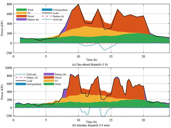
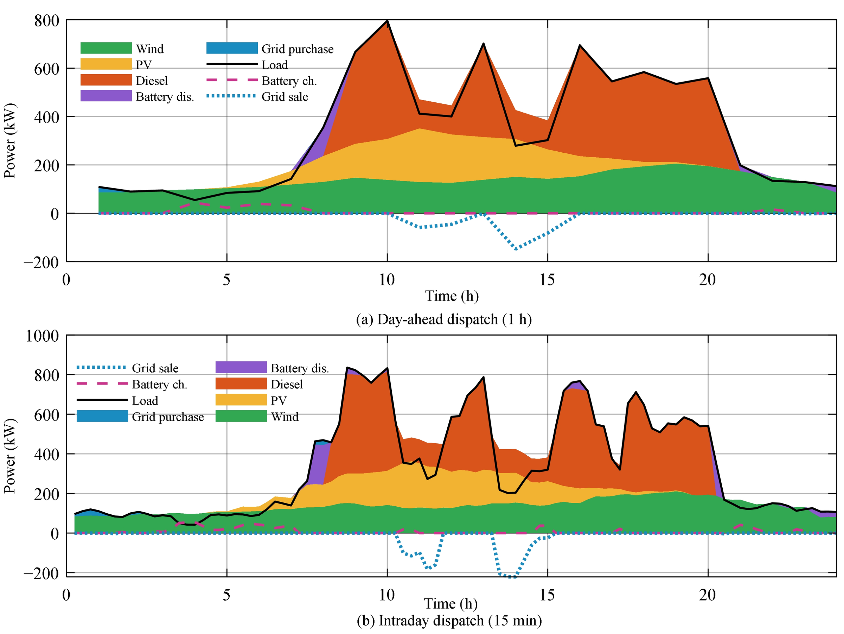
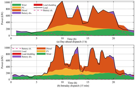
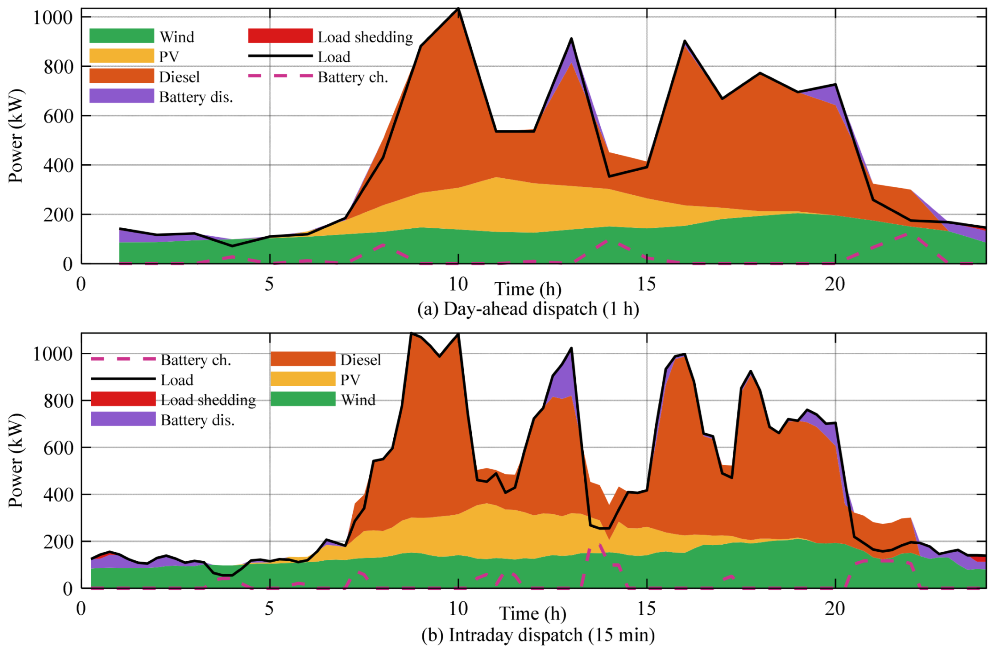
Figure 4 shows the day-ahead (1 h) and intraday (15 min) power-balance dispatch results of the grid-connected microgrid, and Table 4 summarizes the corresponding indicators. The day-ahead layer determines a commitment with a single diesel start and a total cost of 9243.3 CNY. With the commitment fixed, the intraday layer refines the power allocation: the battery cycle energy increases from 159.3 to 216.1 kWh, the grid sale increases from 335.9 to 390.1 kWh and the grid purchase increases from 29.9 to 41.0 kWh, so that the total cost rises by 161.7 CNY (+1.75%). The renewable penetration is 59.45% and 59.44% in the two layers and the energy-based supply reliability is 100% in both, with no load shedding. The absolute day-ahead-versus-intraday cost difference is therefore 161.7 CNY/day, i.e., the finer resolution is not cost-neutral: it buys a more accurate dispatch at a small but quantified cost.

Figure 4. Grid-connected microgrid dispatch results: (a) day-ahead 1 h power balance; (b) intraday 15 min power balance.

Table 4. Grid-connected dual time-scale dispatch results.

Indicator	Day-Ahead (1 h)	Intraday (15 min)
Total cost (CNY)	9243.3	9405.0
Operating cost (CNY)	9022.8	9114.8
Life-cycle cost (CNY)	220.5	290.2
Wind energy (kWh)	3267.9	3267.6
PV energy (kWh)	1528.9	1527.9
Diesel energy (kWh)	3569.8	3620.5
Grid purchase (kWh)	29.9	41.0
Grid sale (kWh)	335.9	390.1
Battery cycle energy (kWh)	159.3	216.1
Renewable penetration (%)	59.45	59.44
Supply reliability (%)	100	100
Diesel starts	1	1

6.3. Islanded Microgrid Dispatch

Figure 5 presents the intraday 15 min dispatch of the islanded microgrid, and Table 5 summarizes the results. The diesel generators supply about 54.7% of the load and renewable energy 45.4%, while the battery cycles 484.7 kWh. The energy not served is 21.5 kWh (0.21% of the load), giving an energy-based reliability of 99.79%; the same schedule has an interval-based service probability of 93.75% with two loss-of-load events and 1.5 h of loss-of-load duration, and the diesel units start at most three times per day. The total cost is 14,978.2 CNY/day, of which 633.1 CNY is life-cycle cost. The results are consistent in magnitude with the values reported in the original engineering case specification (total load 10,349 kWh, renewable 46.0%, diesel 54.2%, reliability 100%), although the differences stem from the randomized data realization and from the load-shedding events introduced by the reserve requirement.

Figure 5. Islanded microgrid intraday 15 min dispatch results.

Table 5. Islanded microgrid dispatch results (intraday 15 min).

Indicator	Value
Total load energy (kWh)	10,451.5
Wind/PV energy (kWh)	3245.1/1498.9
Diesel energy (kWh)	5723.2
Battery cycle energy (kWh)	484.7
Load shedding (kWh)	21.5
Renewable penetration (%)	45.39
Supply reliability (%)	99.79
Diesel starts	3
Total cost (CNY)	14,978.2
Operating/life-cycle cost (CNY)	14,345.0/633.1

6.4. Effect of the Multi-Functional Battery Coordination

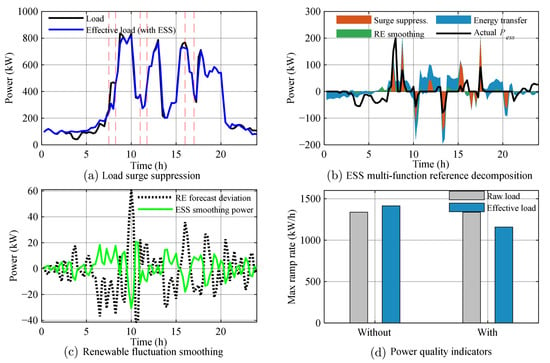
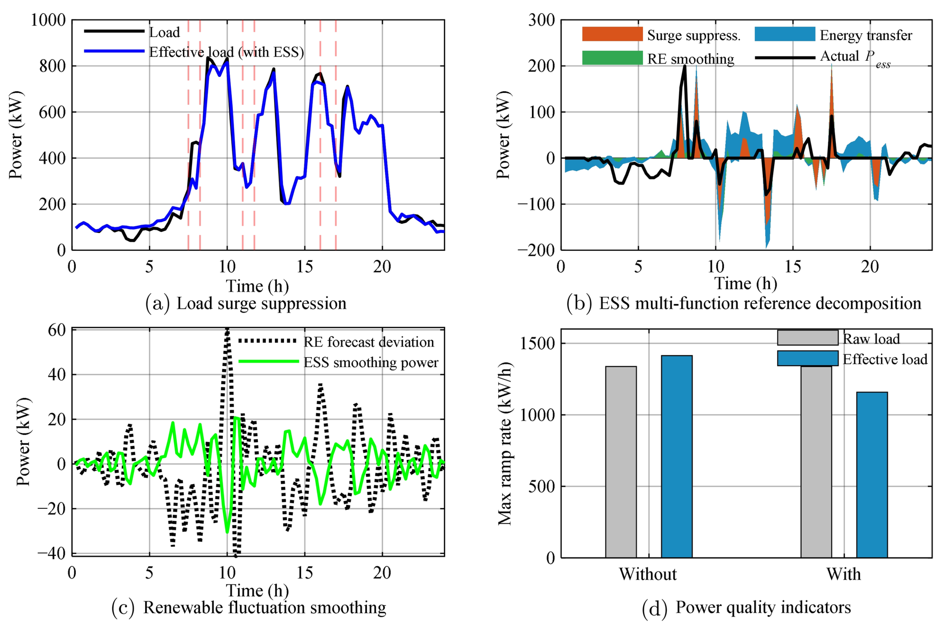
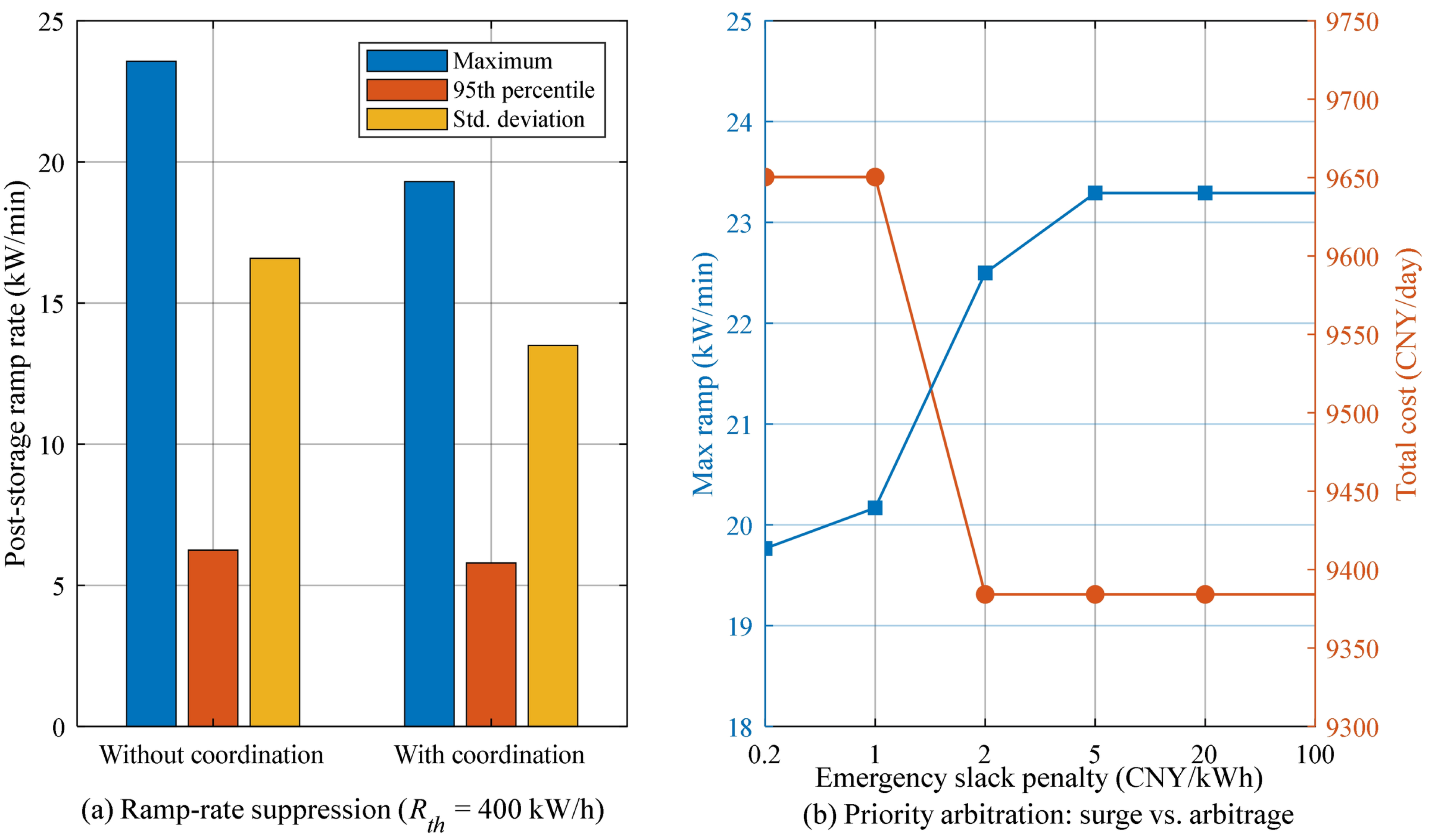
Figure 6 and Table 6 compare the intraday dispatch with and without the multi-functional coordination. The surge events at hours 7.5–8.25, 11.0–11.75 and 16.0–17.0 cause abrupt load steps. Without coordination, the effective load seen by the grid still exhibits a maximum ramp rate of 23.57 kW/min (1413.9 kW/h), which is larger than the raw-load ramp of 22.30 kW/min because unconstrained price arbitrage drives the battery against the load; with coordination, the surge-suppression component responds first and reduces the post-storage maximum ramp rate to 19.31 kW/min (1158.3 kW/h), i.e., by 18.1%; it also reduces the ramp-rate standard deviation from 6.247 to 5.794 kW/min (7.3%) and the 95th percentile from 16.58 to 13.50 kW/min (18.6%). The residual ramp is set by the converter rating: increasing the emergency slack penalty from 2 to 100 CNY/kWh does not reduce it further (Figure 7b); Figure 7a shows the corresponding post-storage ramp-rate statistics. The battery cycle energy decreases slightly from 216.1 to 211.4 kWh, because the surge-suppression request displaces part of the arbitrage cycling. The total cost increases by 126.4 CNY/day (+1.34%), equivalent to about 46,000 CNY/year, or approximately 10,800 CNY/year per kW/min of firm ramp capability that would otherwise have to be provided by additional converter capacity. The priority weights (mean values 0.39, 0.34 and 0.26 over the day, with 18 emergency intervals) demonstrate the dynamic adaptation; a sensitivity study over five normal and three emergency weightings shows that the normal-state weights are non-binding (the cost varies by less than 0.05%), so the emergency weights and the emergency slack penalty are the decisive parameters.

Figure 6. Effect of the multi-functional battery coordination: (a) load surge suppression; (b) coordinated reference decomposition and actual battery power; (c) renewable fluctuation smoothing; (d) power-quality indicators with and without coordination.

Table 6. Comparison of the intraday dispatch with and without multi-functional coordination.

Indicator	Without Coordination	With Coordination
Max ramp rate of raw load (kW/min)	22.30	22.30
Max ramp rate of post-storage load (kW/min)	23.57	19.31
Ramp-rate standard deviation (kW/min)	6.247	5.794
95th-percentile ramp/battery cycle energy (kW/min, kWh)	16.58/216.1	13.50/211.4
Total cost (CNY)	9405.0	9531.5

Figure 7. Effect of the multi-functional coordination and of the priority arbitration. (a) Post-storage ramp-rate statistics with and without coordination; (b) trade-off between ramp suppression and operating cost as the emergency slack penalty increases from 0.2 to 100 CNY/kWh.

6.5. Distributionally Robust Optimization Comparison

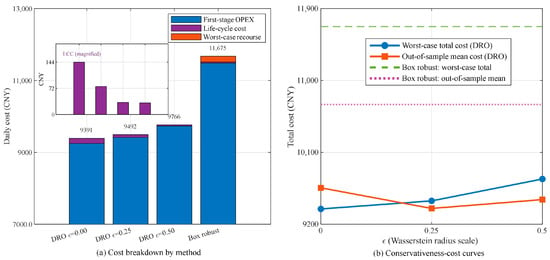
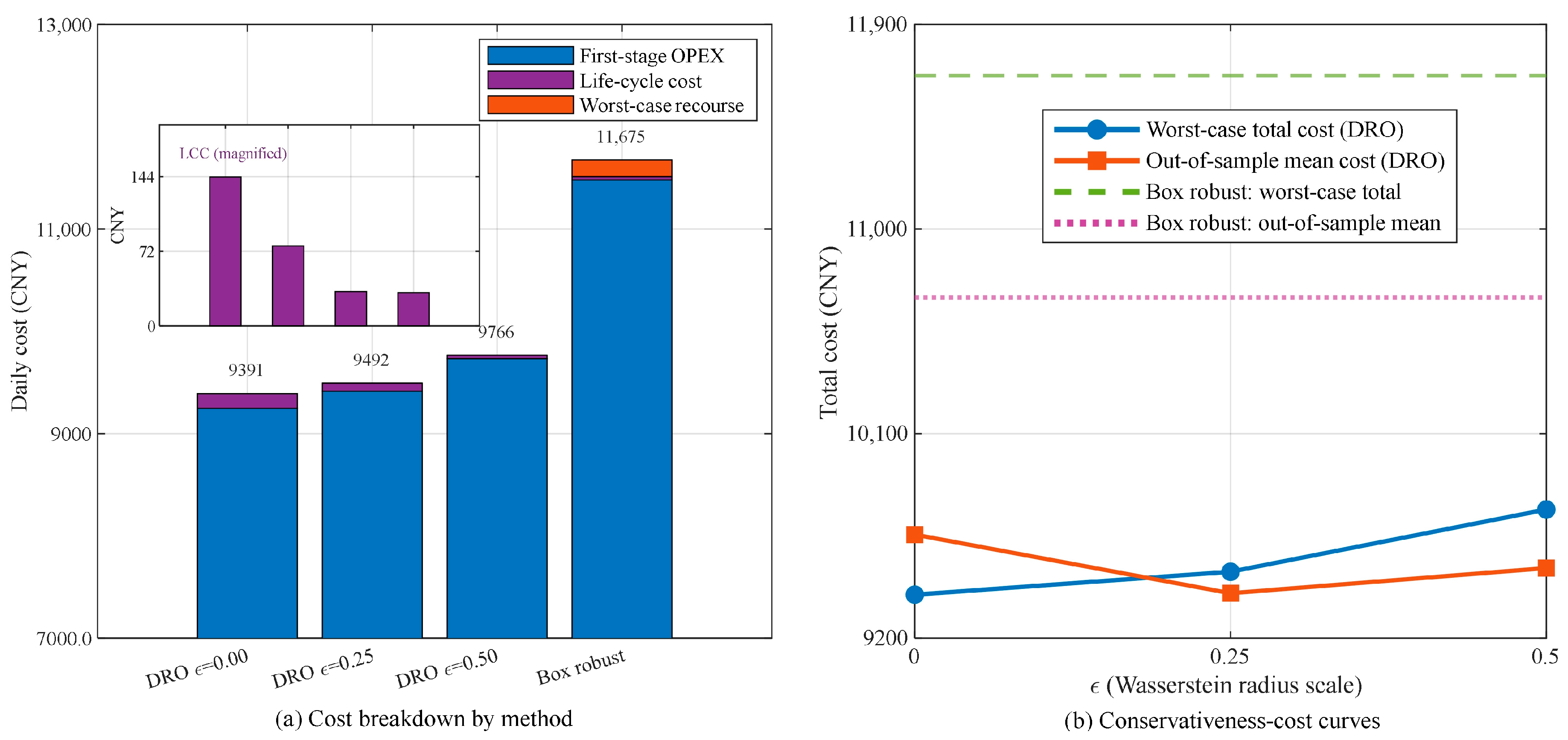
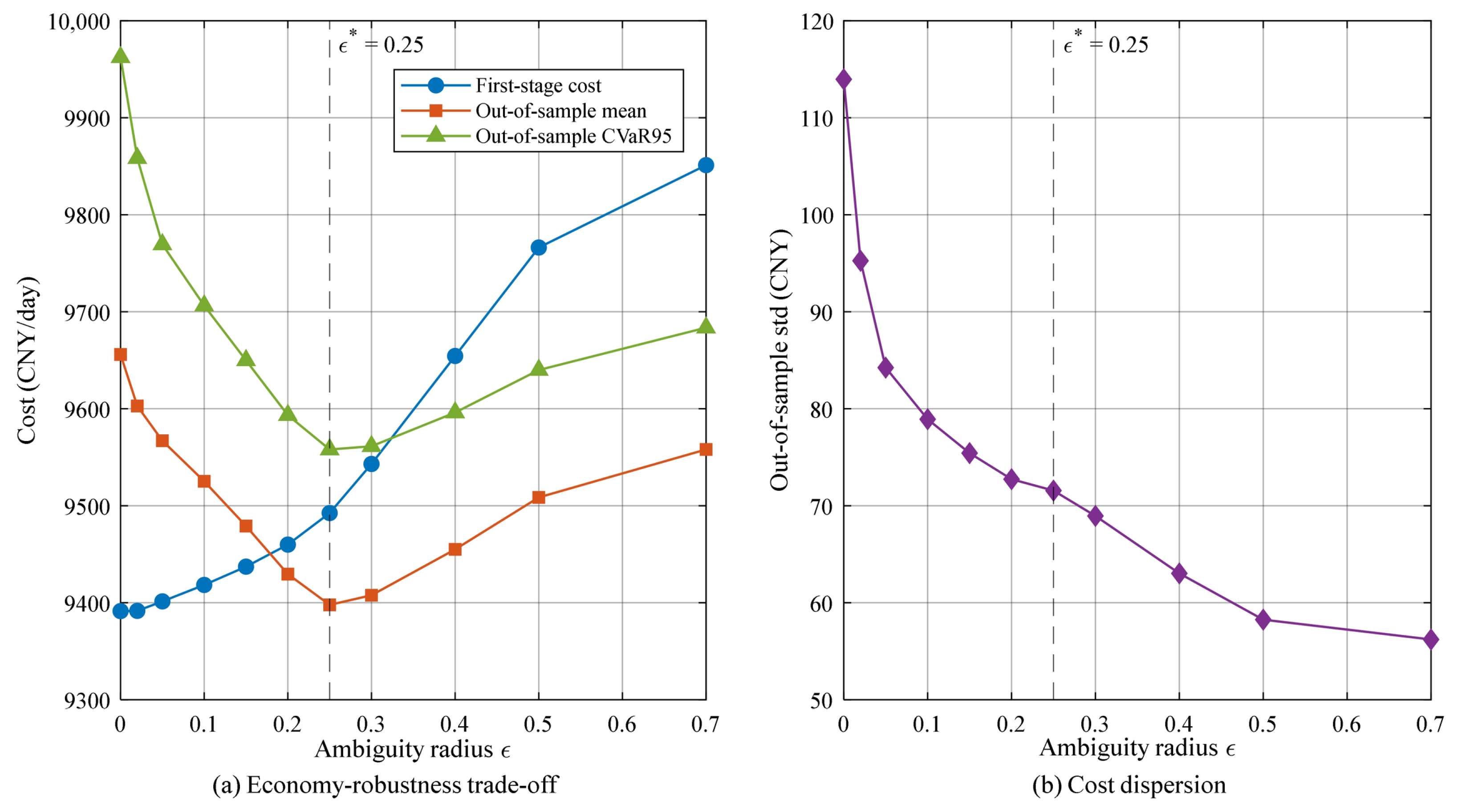
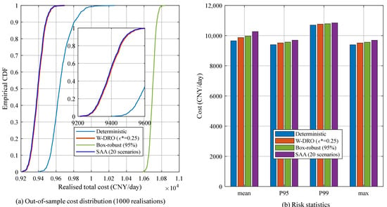
Figure 8 and Table 7 compare the deterministic model (ε = 0), the proposed Wasserstein DRO and the traditional box-type robust optimization at an equivalent coverage. The adaptive radius of Equation (16) yields per-source radii of 2.0–5.0 kW for wind and 1.5–9.8 kW for the load at ε* = 0.25, reflecting the time-varying prediction quality. The deterministic model ignores the uncertainty and yields the lowest reported worst-case total cost (9391.4 CNY), but its worst-case recourse is 0.0 CNY, which is unrealistic because the realized forecast errors inevitably trigger balancing actions. The box-type robust model, which protects against all combinations of the extreme deviations, incurs a worst-case recourse of 805.6 CNY and a total cost of 11,675.1 CNY, i.e., an over-conservative schedule. The proposed DRO lies between the two extremes: its vertex worst-case recourse is 0.0 CNY at the validation-selected radius of 0.25, with a vertex worst-case total cost of 9492.5 CNY. A zero vertex worst case is not a claim that no adverse outcome exists: the nine candidate deviations are absorbed by the recourse re-dispatch within the equipment limits, so the protection of the DRO is carried by the first-stage plan rather than by a positive worst-case recourse term, and realizations that require penalized re-dispatch exceed the reported value (Section 4.4 and Table 8). Furthermore, the out-of-sample evaluation over 1000 new realizations shows that the DRO schedule achieves a mean total cost of 9397.3 CNY, lower than the deterministic 9656.1 CNY and far lower than the box-robust 10,698.3 CNY, confirming that the DRO reaches a better economy-robustness balance without sacrificing the average performance. A 20-scenario stochastic program attains 9393.0 CNY, i.e., within 0.05% of the DRO, so the formal advantage of the DRO rests on its finite-sample guarantee rather than on a superior empirical mean in this case study. Figure 9 reports the complete economy-robustness trade-off as a function of the ambiguity radius, and Figure 10 gives the full out-of-sample cost distribution over the 1000 independent realizations.

Figure 8. Distributionally robust optimization comparison: (a) cost breakdown of the four methods; (b) conservativeness-cost curves (worst-case and out-of-sample).

Table 7. Comparison of the deterministic, distributionally robust, and box-robust dispatch.

Method	ε	First-Stage Cost (CNY)	Worst-Case Recourse (CNY)	Vertex Worst-Case Total (CNY)	Out-of-Sample Mean (CNY)
Deterministic	0	9391.4	0.0	9391.4	9656.1
Wasserstein DRO (ε· = 0.25, validation-selected)	0.25	9492.5	0.0	9492.5	9397.3
Box robust (95% coverage, β = 1.96)	1.96	10,869.5	805.6	11,675.1	10,698.3
Stochastic programming (sample average approximation, SAA; 20 scenarios)	n/a	9506.5	0.0	9506.5	9393.0

Note: the vertex worst-case columns report the value returned by the nine-candidate sub-problem; Section 4.4 defines the three distinct worst-case quantities and Section 6.11 reports the certified bracket between the sample worst case and the support worst case.

Table 8. Out-of-sample cost distribution and tail risk of the four schedules over the same 1000 independent test realizations (seed 7777).

Statistic (CNY/Day)	Deterministic	Wasserstein DRO	Box Robust (95%)	SAA (20 Scenarios)
Mean	9656.1	9397.3	10,698.3	9393.0
Median	9638.3	9394.2	10,697.3	9389.9
Standard deviation	111.9	70.2	36.9	69.9
95th percentile	9870.3	9517.0	10,760.1	9512.1
99th percentile	9968.2	9570.4	10,786.0	9564.1
Maximum	10,267.2	9698.1	10,841.6	9694.2
CVaR at 95%	9940.5	9552.1	10,776.0	9546.7
CVaR at 99%	10,059.3	9603.5	10,799.0	9597.7
Realizations above the reported worst case (%)	100.0	9.2	0.0	5.9

Note: CVaR = conditional value at risk; SAA = sample average approximation. The last row reports the fraction of test realizations whose realized total cost exceeds the worst-case value reported for that schedule in Table 7.

Figure 9. Economy-robustness trade-off with respect to the Wasserstein ambiguity radius. (a) First-stage cost, out-of-sample mean cost and out-of-sample CVaR95 versus the radius, with an interior optimum at ε* = 0.25 selected on the validation set; (b) out-of-sample cost dispersion.

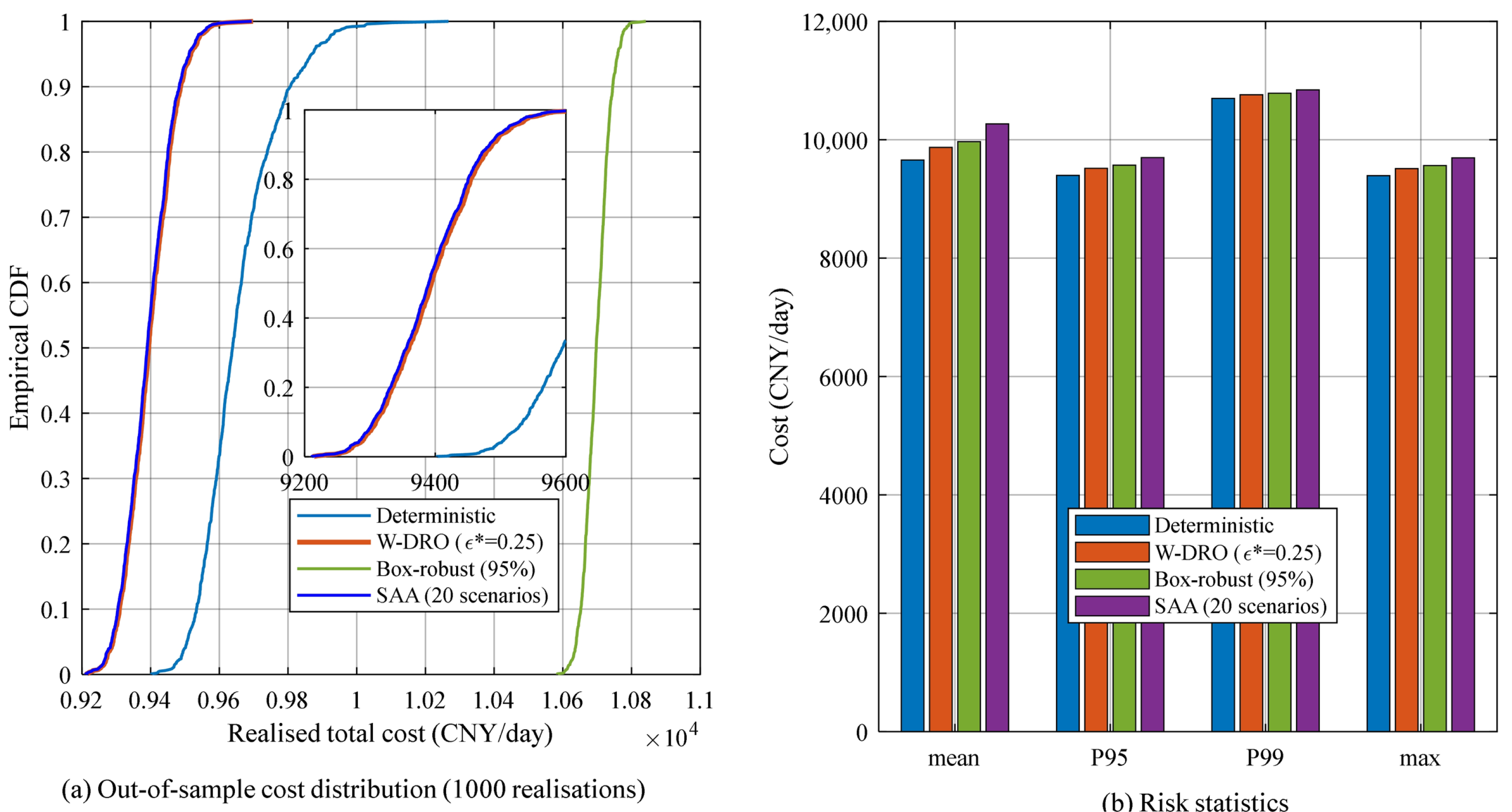
Figure 10. Out-of-sample cost distribution over 1000 independent realizations. (a) Empirical CDF for the deterministic, Wasserstein-DRO, box-robust and stochastic-programming schedules; (b) mean, 95th percentile, 99th percentile and maximum of the realized total cost.

Table 8 reports the complete out-of-sample distribution. The reported worst-case value is exceeded by 9.2% of the DRO realizations, by 5.9% of the stochastic-programming realizations and by 100% of the deterministic realizations; this is expected, because the worst-case quantity is an expectation over the distributions of the ambiguity set, whereas an individual realization is a single draw that can fall outside the standardized region in which the recourse re-dispatches without penalty. The box-robust value is exceeded by none of the realizations, because its uncertainty set is calibrated at 95% single-source coverage and priced at the extreme combination of the three sources. In the grid-connected case no realization of any schedule sheds load, so the energy-not-served and loss-of-load indices are zero for all four benchmarks and are reported for the islanded case in Section 6.7, where they are non-zero; renewable curtailment is reported in Table 6 for the coordination variants and in Table 5 for the islanded case.

6.6. Effect of the Life-Cycle-Cost-Aware Dispatch

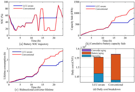
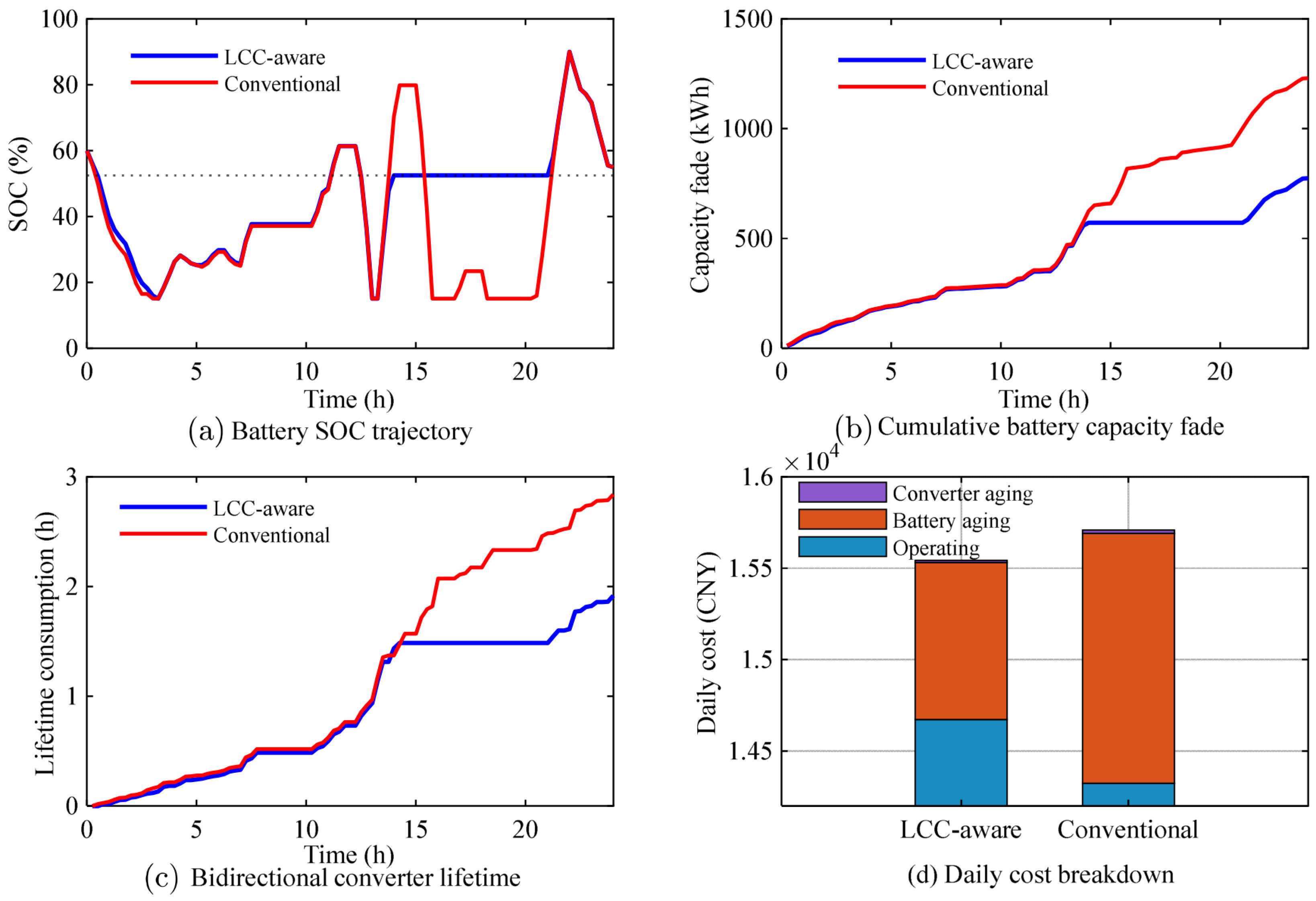
Figure 11 and Table 9 compare the islanded dispatch with and without the life-cycle-cost terms in Equations (27) and (28). For the islanded case the marine-grade battery unit investment cost is 4000 CNY/kWh (including the dedicated BMS (battery management system), protection and installation). The LCC-aware (life-cycle-cost-aware) dispatch raises the operating cost by 252.3 CNY/day (from 14,311.0 to 14,563.3 CNY, +1.76%) but reduces the battery aging cost from 1367.6 to 860.2 CNY (−37.1%), the converter stress cost from 17.7 to 12.0 CNY (−32.5%), the equivalent aging throughput from 1230.8 to 774.2 kWh (−37.1%), the equivalent capacity fade from 0.1368% to 0.0860% per day (−37.1%) and the converter equivalent stress hours from 2.839 to 1.916 h/day (−32.5%). The total cost therefore decreases from 15,696.3 to 15,435.5 CNY (−1.66%). As shown in Figure 11a, the LCC-aware SOC trajectory is drawn toward the mid-range value SOC_mid, which reduces the SOC-stress term, and the battery cycle energy is moderated from 512.0 to 327.5 kWh. The economic reconciliation over the asset horizon is unambiguous: the avoided life-cycle cost (about 187,300 CNY/year under the surrogate) exceeds the additional operating expenditure (92,100 CNY/year) by a factor of about 2.0, and the break-even degradation cost is 0.68 CNY per kWh of throughput, i.e., the LCC-aware dispatch is justified whenever the true battery degradation cost exceeds that value (the assumed value is 1.11 CNY/kWh for the marine-grade unit).

Figure 11. Effect of the life-cycle-cost-aware dispatch: (a) battery SOC trajectory; (b) cumulative capacity fade; (c) converter lifetime consumption; (d) daily cost breakdown.

Table 9. Comparison of the LCC-aware and conventional dispatch (islanded).

Indicator	LCC-Aware	Conventional
Operating cost (CNY)	14,563.3	14,311.0
Battery aging cost (CNY)	860.2	1367.6
Converter stress cost (CNY)	12.0	17.7
Equivalent aging throughput (kWh)	774.2	1230.8
Converter power-variation stress (equivalent hours/day)	1.916	2.839
Battery cycle energy (kWh)	327.5	512.0
Total cost (operating + life-cycle, CNY)	15,435.5	15,696.3

6.7. Islanded Operation: Event and Reserve Analysis

Because the islanded case is a planned islanded campaign, the initiating condition is a scheduled disconnection of the 400 kW grid interface at 00:00 with an initial SOC of 0.60. Over the islanded day the diesel units generate 5723.2 kWh in three start-ups, the renewable energy available is 4797.3 kWh of which 4744.0 kWh is served and 53.3 kWh curtailed, and the BESS cycles 484.7 kWh. The reserve requirement derived in Section 3.6 is 175 kW (95th-percentile net forecast uncertainty), versus 128 kW for the largest surge; 240 kW is available from the BESS, with a minimum instantaneous power reserve of 91 kW and an energy reserve of 147 kWh against a requirement of 118 kWh; the requirement is therefore satisfied but consumes up to 73% of the converter rating. Non-critical marine test loads are shed first: the energy not served is 21.5 kWh in two events totalling 1.5 h. A single-machine equivalent swing model (2H S_rated/f₀ · df/dt = ΔP with H = 5 s and S_rated = 1500 kW) gives a maximum frequency deviation of 0.21 Hz and a maximum rate of change of frequency of 0.031 Hz/s, both within the ±0.2 Hz steady-state and ±0.5 Hz transient limits; only the diesel units contribute inertia, which is stated as an assumption. The schedule keeps SOC(N + 1) within ±0.05 of SOC₀, so the microgrid can resynchronise without a pre-recharge step.

6.8. Dual Time-Scale Comparison

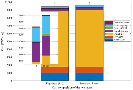
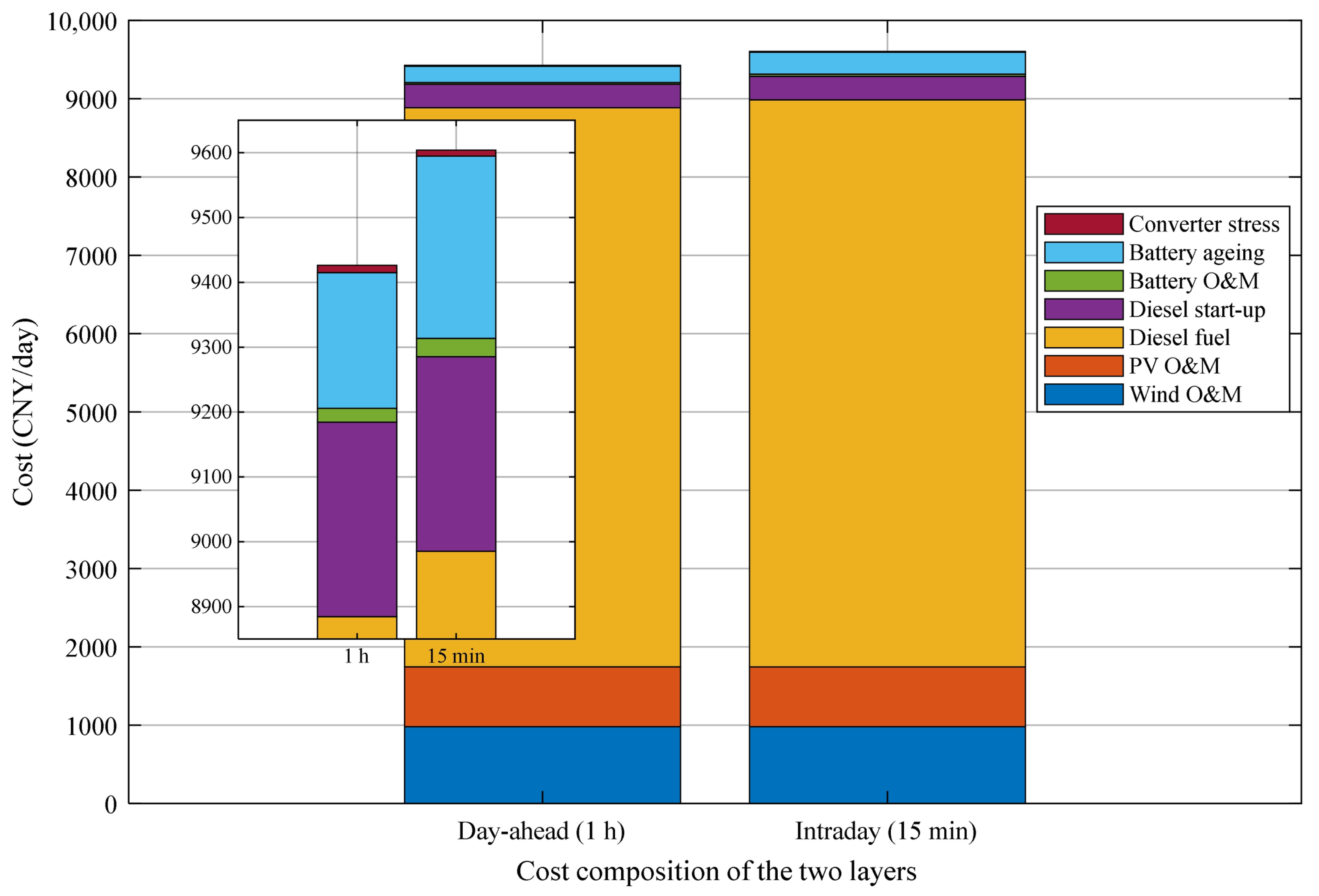
Figure 12 compares the cost composition of the two layers and Table 4 gives the detailed indicators. The day-ahead layer obtains the unit commitment with one diesel start and a total cost of 9243.3 CNY, whereas the intraday layer, under the fixed commitment, increases the battery cycle energy from 159.3 to 216.1 kWh and the grid sale from 335.9 to 390.1 kWh while increasing the grid purchase from 29.9 to 41.0 kWh. The intraday layer therefore raises the life-cycle cost (from 220.5 to 290.2 CNY) while the converter stress cost changes little, and the total cost rises by 161.7 CNY (+1.75%). The dual time-scale coordination thus implements a “day-ahead commits, intraday dispatches” scheme with a quantified accuracy-cost trade-off.

Figure 12. Cost composition comparison of the day-ahead (1 h) and intraday (15 min) layers.

6.9. Simultaneous Operation of All Four Mechanisms and Ablation

Section 6.4, Section 6.5, Section 6.6, Section 6.7 and Section 6.8 evaluate the mechanisms one at a time; this section reports the configuration in which all four operate together, together with an ablation. To make the comparison an ablation rather than a comparison of runs, the eight configurations of Table 10 share the same data realization, the same 200 training and 700 validation samples, the same ambiguity radius (ε* = 0.25), the same day-ahead commitment (one diesel start) and the same metric definitions; only the set of active mechanisms changes. The integrated schedule F1 activates the multi-functional battery reference of Section 3, the Wasserstein DRO of Section 4, the life-cycle terms of Section 5 and the dual time-scale structure of Section 5.4.

Table 10 reports the eight configurations. The fully integrated schedule F1 attains a maximum post-storage ramp of 19.31 kW/min and a planned cost of 9661.6 CNY/day, of which 155.4 CNY is life-cycle cost. Removing the battery degradation term (F3) lowers the planned operating cost to 9135.3 CNY/day but raises the life-cycle cost to 797.1 CNY/day, so the total rises by 270.9 CNY/day (+2.8%) and the out-of-sample CVaR95 of the recourse cost rises from 68.8 to 218.6 CNY/day; removing both life-cycle terms (F4) has the same effect, more strongly (+304.8 CNY/day, CVaR95 231.6 CNY/day). Removing the coordination (F5) raises the maximum ramp from 19.31 to 23.57 kW/min (+22.1%) and lowers the planned cost by 111.2 CNY/day, i.e., the coordination is bought with 111.2 CNY/day and, equivalently, with a firm-ramp capability of 4.26 kW/min. Removing the DRO (F6) produces by far the largest deterioration of the tail: the planned cost falls by 134.9 CNY/day, but the out-of-sample CVaR95 rises from 68.8 to 609.2 CNY/day (8.9 times) and the mean recourse cost from −92.2 to +291.5 CNY/day, because a deterministic plan must re-dispatch repeatedly once the realization departs from the forecast. The single time-scale variant (F7) is 107.6 CNY/day cheaper and, on this realization, its out-of-sample tail is marginally smaller (66.9 against 68.8 CNY/day); the dual time-scale structure is therefore justified by the operational requirement that the commitment be frozen 24 h ahead, not by a cost or tail-risk gain, and we say so rather than claim a benefit that is not present. The unintegrated baseline F8 is 72.7 CNY/day cheaper in plan but has a 22.1% higher ramp and 9.9 times the CVaR95 of F1.

The ablation therefore separates the two objectives. The coordination dominates the power-quality indicator (19.31 against 23.57 kW/min), whereas the DRO and the life-cycle terms dominate the out-of-sample tail (CVaR95 68.8 against 609.2 and 231.6 CNY/day); no single mechanism improves both, which is the reason for combining them. The difference between F1 and F8 is the effect of the four mechanisms taken together and is the quantity on which the integrated claim of this paper rests.

The same integrated configuration was also solved for the islanded case of Section 6.3. With all four mechanisms active the maximum post-storage ramp is 22.176 kW/min against 25.387 kW/min without the coordination (−12.6%), the life-cycle cost is 1005.3 against 857.7 CNY/day, the planned total cost 15,712.9 against 15,600.6 CNY/day (+0.72%), the out-of-sample mean recourse cost 453.82 against 463.38 CNY/day and the CVaR95 573.62 against 584.13 CNY/day. In the islanded case the coordination therefore improves both the ramp and the out-of-sample tail, but it costs 147.6 CNY/day of additional battery aging, because the surge request and the reserve requirement together force more cycling; this is reported as a trade-off rather than as an improvement.

Because the integrated schedule also carries the coordination reference and the life-cycle terms, its planned cost is not directly comparable with the DRO benchmark of Table 7, which has neither; the comparison of interest in this section is across the rows of Table 10, all of which share the same protocol.

Table 10. Ablation of the four mechanisms on the grid-connected case (identical data, commitment and metric definitions in all rows).

Configuration	Max Ramp (kW/min)	Ramp Std (kW/min)	LCC Cost (CNY/Day)	Total Cost (CNY/Day)	Δ vs. F1 (CNY/Day)	OOS Mean Recourse (CNY/Day)	OOS CVaR95 (CNY/Day)
F1 all mechanisms	19.31	5.865	155.4	9661.6	-	−92.2	68.8
F2 w/o converter LCC	19.31	5.843	168.1	9662.7	+1.1	−88.2	73.9
F3 w/o battery degradation	18.84	4.885	797.1	9932.4	+270.9	46.6	218.6
F4 w/o both life-cycle terms	15.75	4.892	831.0	9966.3	+304.8	54.8	231.6
F5 w/o coordination	23.57	6.502	123.0	9550.4	−111.2	−84.6	78.9
F6 w/o DRO (deterministic)	19.31	5.794	290.5	9526.7	−134.9	291.5	609.2
F7 single time scale	19.31	5.882	147.0	9554.0	−107.6	−93.7	66.9
F8 no coordination, no DRO, no LCC	23.57	5.606	855.5	9588.9	−72.7	347.4	682.8

Note: F1 activates all four mechanisms; F2 removes the converter life-cycle term, F3 the battery degradation term, F4 both life-cycle terms, F5 the multi-functional coordination, F6 the DRO and F7 the day-ahead layer (single 15 min time scale); F8 keeps only the dual time-scale structure. LCC = life-cycle cost; OOS = out-of-sample over 500 independent realizations. The OOS columns report the recourse cost, i.e., the cost incurred in excess of the planned cost, and are therefore not comparable with the total-cost columns of Table 8.

Table 10. Ablation of the four mechanisms on the grid-connected case (identical data, commitment and metric definitions in all rows).

Configuration	Max Ramp (kW/min)	Ramp Std (kW/min)	LCC Cost (CNY/Day)	Total Cost (CNY/Day)	Δ vs. F1 (CNY/Day)	OOS Mean Recourse (CNY/Day)	OOS CVaR95 (CNY/Day)
F1 all mechanisms	19.31	5.865	155.4	9661.6	-	−92.2	68.8
F2 w/o converter LCC	19.31	5.843	168.1	9662.7	+1.1	−88.2	73.9
F3 w/o battery degradation	18.84	4.885	797.1	9932.4	+270.9	46.6	218.6
F4 w/o both life-cycle terms	15.75	4.892	831.0	9966.3	+304.8	54.8	231.6
F5 w/o coordination	23.57	6.502	123.0	9550.4	−111.2	−84.6	78.9
F6 w/o DRO (deterministic)	19.31	5.794	290.5	9526.7	−134.9	291.5	609.2
F7 single time scale	19.31	5.882	147.0	9554.0	−107.6	−93.7	66.9
F8 no coordination, no DRO, no LCC	23.57	5.606	855.5	9588.9	−72.7	347.4	682.8

Note: F1 activates all four mechanisms; F2 removes the converter life-cycle term, F3 the battery degradation term, F4 both life-cycle terms, F5 the multi-functional coordination, F6 the DRO and F7 the day-ahead layer (single 15 min time scale); F8 keeps only the dual time-scale structure. LCC = life-cycle cost; OOS = out-of-sample over 500 independent realizations. The OOS columns report the recourse cost, i.e., the cost incurred in excess of the planned cost, and are therefore not comparable with the total-cost columns of Table 8.

6.10. Discussion

The case studies jointly demonstrate the three innovations. First, the multi-functional coordination resolves the function conflicts of a finite battery and improves the power quality at a negligible cost penalty, which is essential for the frequently starting/stopping test loads in offshore engineering microgrids. Second, the Wasserstein DRO with adaptive radii provides a principled balance between economy and robustness: compared with the deterministic model, it avoids the risk of unmodeled worst cases, and compared with the box-type robust model, it avoids over-conservatism, with the out-of-sample results confirming that the balance does not degrade the average performance. Third, the life-cycle-cost-aware dual time-scale dispatch explicitly charges battery degradation and converter lifetime consumption to the schedule, yielding substantial lifetime benefits at a moderate operating-cost increase (+1.76%). The mechanisms are evaluated separately in Section 6.4, Section 6.5, Section 6.6, Section 6.7 and Section 6.8 to isolate their individual effects, and they are also evaluated together in Section 6.9, where the integrated schedule is compared with seven ablations under one protocol; the integrated schedule attains the lowest ramp of the configurations that keep the coordination active and the second-lowest out-of-sample tail of the eight configurations, behind only the single-time-scale variant, which does not respect the 24 h commitment. Note that the current model adopts a simplified converter lifetime model proportional to the power-variation intensity; more detailed thermal-cycling models based on junction-temperature profiles can be embedded when the corresponding mission-profile data are available. The scalability of the C&CG algorithm for larger systems, as well as the joint scheduling with other flexible resources, is left for future work.

6.11. Algorithmic Evidence, Computational Feasibility and Solver Independence

All optimization models are implemented in MATLAB with YALMIP and solved with the MATLAB Optimization Toolbox MILP solver at a relative gap of 1 × 10⁻⁴ on an AMD Ryzen 9 9950X3D workstation (16 physical cores). Because Gurobi’s academic license is not available in the authors’ region, the solver was changed relative to the first submission; to establish that this does not affect any reported result, every model instance was independently solved with IBM CPLEX 12.10 through a direct matrix interface, and the objectives agree to within 2 × 10⁻⁹ (Table 11). The CPLEX verification also shows that the islanded instances are solved 3–11 times faster by CPLEX, which is a computational remark only. The algorithm comparison is reported in Table 11 as well: the improved C&CG with nine vertex candidates converges in two iterations and 18 recourse LP evaluations, whereas a variant enumerating all 200 training samples requires 400 evaluations and returns a vertex-to-sample gap of 202.1 CNY (2.1%) at ε = 0.20 (9459.93 against 9662.06 CNY), because the empirical samples lie farther from the center than the vertices of the ε-box and therefore answer a different, more conservative question. The sample value is itself a lower bound of the worst-case expectation, and the support worst case at the same radius closes the bracket from above: at a half-width of one standardized unit the box-robust schedule costs 10,349.4 CNY, so the worst-case expectation of the proposed model lies in [9662.06, 10,349.4] CNY and the nine-vertex value under-states the upper end of the bracket by 8.6%. In the receding-horizon campaign the intraday problem is re-solved 24 times over shrinking horizons; the mean solution time is 6.9 s and the maximum 11.9 s, i.e., at most 1.3% of the 900 s decision interval. The solution time grows approximately linearly with the number of slots (0.9 s at N = 24, 1.6 s at N = 48 and 3.4 s at N = 96 for a single intraday solve), so the scheme remains real-time feasible for substantially larger models.

Table 11. Solver cross-validation, algorithm comparison and computation times (AMD Ryzen 9 9950X3D, 16 physical cores).

Model Instance/Metric	MATLAB Intlinprog	IBM CPLEX 12.10	Relative Difference
G1 grid intraday 15 min, objective (CNY)	9391.3800	9391.3800	3.9 × 10−16
G2 grid intraday 15 min without LCC, objective (CNY)	8729.2964	8729.2964	4.3 × 10−14
G3 grid day-ahead 1 h, objective (CNY)	9243.3213	9243.3213	3.9 × 10−16
I1 island intraday 15 min with LCC, objective (CNY)	14,905.3237	14,905.3237	7.3 × 10−16
I2 island intraday 15 min without LCC, objective (CNY)	14,237.0411	14,237.0411	1.8 × 10−9
Model size G1 (rows × columns, binaries)	5470 × 2209, 864	same	-
Model size I1 (rows × columns, binaries)	4702 × 1921, 768	same	-
Solution time, island intraday with LCC (s)	31.95	2.88	-
Improved C&CG (9 vertex candidates): iterations/recourse LP evaluations	2/18	-	-
Conventional C&CG (200 samples): iterations/recourse LP evaluations	2/400	-	-
Improved vs. conventional worst-case cost (CNY)	9459.93 vs. 9662.06	-	+2.1%
Receding-horizon campaign, mean/maximum time (s)	6.9/11.9	-	1.3% of 900 s

Table 11. Solver cross-validation, algorithm comparison and computation times (AMD Ryzen 9 9950X3D, 16 physical cores).

Model Instance/Metric	MATLAB Intlinprog	IBM CPLEX 12.10	Relative Difference
G1 grid intraday 15 min, objective (CNY)	9391.3800	9391.3800	3.9 × 10−16
G2 grid intraday 15 min without LCC, objective (CNY)	8729.2964	8729.2964	4.3 × 10−14
G3 grid day-ahead 1 h, objective (CNY)	9243.3213	9243.3213	3.9 × 10−16
I1 island intraday 15 min with LCC, objective (CNY)	14,905.3237	14,905.3237	7.3 × 10−16
I2 island intraday 15 min without LCC, objective (CNY)	14,237.0411	14,237.0411	1.8 × 10−9
Model size G1 (rows × columns, binaries)	5470 × 2209, 864	same	-
Model size I1 (rows × columns, binaries)	4702 × 1921, 768	same	-
Solution time, island intraday with LCC (s)	31.95	2.88	-
Improved C&CG (9 vertex candidates): iterations/recourse LP evaluations	2/18	-	-
Conventional C&CG (200 samples): iterations/recourse LP evaluations	2/400	-	-
Improved vs. conventional worst-case cost (CNY)	9459.93 vs. 9662.06	-	+2.1%
Receding-horizon campaign, mean/maximum time (s)	6.9/11.9	-	1.3% of 900 s

7. Conclusions

This paper proposed a data-driven distributionally robust economic dispatch method for offshore engineering microgrids. The method integrates three coordinated techniques:

(i)

A multi-functional coordination model of the battery energy storage system that unifies test-load surge suppression, renewable fluctuation smoothing, and long-term energy transfer through priority-based dynamic weighting and a total-power-constrained allocation, and embeds the coordinated reference into the dispatch as a tracking constraint with a reserved margin;

(ii)

A two-stage Wasserstein distributionally robust optimization with adaptive ambiguity radii and an improved column-and-constraint generation algorithm for the correlated wind, PV, and test-load uncertainties;

(iii)

A life-cycle-cost-aware objective with linearized battery capacity-fade and converter lifetime-consumption terms, integrated into a dual time-scale (1 h day-ahead/15 min intraday) scheduling framework.

Case studies on grid-connected and islanded offshore engineering microgrids showed that the multi-functional coordination reduces the post-storage maximum load ramp rate from 23.57 to 19.31 kW/min (−18.1%) and its standard deviation from 6.25 to 5.79 kW/min (−7.3%) at an operating-cost increase of 126.4 CNY/day (+1.34%), while the reserved power and energy margin satisfies a requirement of 175 kW and 118 kWh derived from the 95th-percentile forecast uncertainty; the Wasserstein DRO reduces the out-of-sample mean cost from 9656.1 to 9397.3 CNY (−2.7%) and the CVaR95 from 9940.5 to 9552.1 CNY (−3.9%) over 1000 independent realizations, compared with 10,698.3 CNY for an equivalently calibrated box-robust schedule; and the life-cycle-cost-aware dispatch reduces the equivalent battery capacity fade by 37.1% and the converter power-variation stress by 32.5% at an operating-cost increase of 1.76%, while keeping the energy-based supply reliability at 99.79–100%. All results were reproduced with two independent MILP solvers whose objectives agree to within 2 × 10⁻⁹. When the four mechanisms operate simultaneously, the integrated schedule attains a maximum post-storage ramp of 19.31 kW/min and, among the eight configurations of the ablation, the second-lowest out-of-sample tail; removing the coordination raises the ramp by 22.1% and removing the DRO multiplies the out-of-sample CVaR95 of the recourse cost by 8.9. Three limitations are stated explicitly. First, the quantity optimized by the DRO is a worst-case expectation over the ambiguity set rather than a bound on individual realizations, and 9.2% of the test realizations exceed it. Second, the linearized aging surrogates rank schedules reliably but do not predict absolute life, because the conversion coefficients must be recalibrated against field aging data; the life-cycle cost figures should therefore be read as relative. Third, on this test set a 20-scenario stochastic program attains a mean cost within 0.05% of the proposed DRO, so the formal advantage of the DRO rests on its finite-sample guarantee rather than on a superior empirical mean in this particular case study. Future work will extend the framework to multi-microgrid coordination with peer-to-peer energy trading, embed thermal-cycling-based converter models with humidity acceleration, and integrate the scheduling with the real-time control of the bidirectional converters.

References

- Nivolianiti, E.; Karnavas, Y.L.; Charpentier, J.F. Energy management of shipboard microgrids integrating energy storage systems: A review. Renew. Sustain. Energy Rev. 2024, 189, 114012. [Google Scholar] [CrossRef] [Scilit]
- Ray, A.; Rajashekara, K. Electrification of offshore oil and gas production: Architectures and power conversion. Energies 2023, 16, 5812. [Google Scholar] [CrossRef] [Scilit]
- Chen, H.; Wang, Y.; Wang, Q.; Song, H.; Li, J. An overview of green offshore electric energy systems: Types, advances, potential challenges, and solutions. Int. J. Green Energy 2025, 22, 2583–2596. [Google Scholar] [CrossRef] [Scilit]
- Wyckoff, K.; Moazeni, F.; Khazaei, J.; Banerjee, A. Economic dispatch of offshore renewable energy resources for islanded communities with optimal storage sizing. Renew. Energy 2025, 241, 122153. [Google Scholar] [CrossRef] [Scilit]
- Parhizi, S.; Lotfi, H.; Khodaei, A.; Bahramirad, S. State of the art in research on microgrids: A review. IEEE Access 2015, 3, 890–925. [Google Scholar] [CrossRef] [Scilit]
- Vinothine, S.; Widanagama Arachchige, L.N.; Rajapakse, A.D.; Kaluthanthrige, R. Microgrid energy management and methods for managing forecast uncertainties. Energies 2022, 15, 8525. [Google Scholar] [CrossRef] [Scilit]
- Olivares, D.E.; Mehrizi-Sani, A.; Etemadi, A.H.; Canizares, C.A.; Iravani, R.; Kazerani, M.; Hajimiragha, A.H.; Gomis-Bellmunt, O.; Saeedifard, M.; Palma-Behnke, R.; et al. Trends in microgrid control. IEEE Trans. Smart Grid 2014, 5, 1905–1919. [Google Scholar] [CrossRef] [Scilit]
- Liu, X.; Zhao, T.; Deng, H.; Wang, P.; Liu, J.; Blaabjerg, F. Microgrid energy management with energy storage systems: A review. CSEE J. Power Energy Syst. 2023, 9, 483–504. [Google Scholar] [CrossRef] [Scilit]
- Su, W.; Wang, J.; Roh, J. Stochastic energy scheduling in microgrids with intermittent renewable energy resources. IEEE Trans. Smart Grid 2014, 5, 1876–1883. [Google Scholar] [CrossRef] [Scilit]
- Bertsimas, D.; Brown, D.B.; Caramanis, C. Theory and applications of robust optimization. SIAM Rev. 2011, 53, 464–501. [Google Scholar] [CrossRef] [Scilit]
- Jiang, R.; Wang, J.; Guan, Y. Robust unit commitment with wind power and pumped storage hydro. IEEE Trans. Power Syst. 2012, 27, 800–810. [Google Scholar] [CrossRef] [Scilit]
- Zeng, B.; Zhao, L. Solving two-stage robust optimization problems using a column-and-constraint generation method. Oper. Res. Lett. 2013, 41, 457–461. [Google Scholar] [CrossRef] [Scilit]
- Wei, W.; Liu, F.; Mei, S. Distributionally robust co-optimization of energy and reserve dispatch. IEEE Trans. Sustain. Energy 2016, 7, 289–300. [Google Scholar] [CrossRef] [Scilit]
- Esfahani, P.M.; Kuhn, D. Data-driven distributionally robust optimization using the Wasserstein metric: Performance guarantees and tractable reformulations. Math. Program. 2018, 171, 115–166. [Google Scholar] [CrossRef] [Scilit]
- Zhao, C.; Guan, Y. Data-driven risk-averse stochastic optimization with Wasserstein metric. Oper. Res. Lett. 2018, 46, 262–267. [Google Scholar] [CrossRef] [Scilit]
- Xu, D.; Wu, Z. Enhanced frequency aware microgrid scheduling towards seamless islanding under frequency support of heterogeneous resources: A distributionally robust chance constrained approach. Int. J. Electr. Power Energy Syst. 2024, 162, 110310. [Google Scholar] [CrossRef] [Scilit]
- Shi, Z.; Zhang, T.; Liu, Y.; Feng, Y.; Wang, R.; Huang, S. Optimal design and operation of islanded multi-microgrid system with distributionally robust optimization. Electr. Power Syst. Res. 2023, 221, 109437. [Google Scholar] [CrossRef] [Scilit]
- Zhang, X.; Yang, Y.; Zhao, H.; Luo, Y.; Xu, X. Two-stage optimal scheduling of an islanded microgrid considering uncertainties of renewable energy. Int. J. Electr. Power Energy Syst. 2024, 162, 110324. [Google Scholar] [CrossRef] [Scilit]
- Hou, H.; Wang, Q.; Xue, M. Two-stage economic day-ahead dispatch of an islanded microgrid considering uncertainty and demand response. Power Syst. Prot. Control. 2022, 50, 73–85. (In Chinese) [Google Scholar]
- Wei, M.; Wu, Y.; Li, Y.; Long, M.; Zhong, J.; Li, Y. Day-ahead economic operation model of microgrid and its solving method based on distributed robust optimization. Proc. CSU-EPSA 2022, 34, 81–90. [Google Scholar]
- Gui, Y.; Nainar, K.; Bendtsen, J.D.; Diewald, N.; Iov, F.; Yang, Y.; Blaabjerg, F.; Xue, Y.; Liu, J.; Hong, T.; et al. Voltage support with PV inverters in low-voltage distribution networks: An overview. IEEE J. Emerg. Sel. Top. Power Electron. 2024, 12, 1503–1522. [Google Scholar] [CrossRef] [Scilit]
- Shi, Y.; Xu, B.; Wang, D.; Zhang, B. Using battery storage for peak shaving and frequency regulation: Joint optimization for superlinear gains. IEEE Trans. Power Syst. 2018, 33, 2882–2894. [Google Scholar] [CrossRef] [Scilit]
- Tadie, A.T.; Guo, Z.; Xu, Y. Hybrid model-based BESS sizing and control for wind energy ramp rate control. Energies 2022, 15, 9244. [Google Scholar] [CrossRef] [Scilit]
- Xu, B.; Oudalov, A.; Ulbig, A.; Andersson, G.; Kirschen, D.S. Modeling of lithium-ion battery degradation for cell life assessment. IEEE Trans. Smart Grid 2018, 9, 1131–1140. [Google Scholar] [CrossRef] [Scilit]
- Wang, H.; Liserre, M.; Blaabjerg, F. Toward reliable power electronics: Challenges, design tools, and opportunities. IEEE Ind. Electron. Mag. 2013, 7, 17–26. [Google Scholar] [CrossRef] [Scilit]
- Yang, S.; Bryant, A.; Mawby, P.; Xiang, D.; Ran, L.; Tavner, P. An industry-based survey of reliability in power electronic converters. IEEE Trans. Ind. Appl. 2011, 47, 1441–1451. [Google Scholar] [CrossRef] [Scilit]
- Wang, J.; Liu, P.; Hicks-Garner, J.; Sherman, E.; Soukazian, S.; Verbrugge, M.; Tataria, H.; Musser, J.; Finamore, P. Cycle-life model for graphite-LiFePO4 cells. J. Power Sources 2011, 196, 3942–3948. [Google Scholar] [CrossRef] [Scilit]
Disclaimer/Publisher’s Note: The statements, opinions and data contained in all publications are solely those of the individual author(s) and contributor(s) and not of MDPI and/or the editor(s). MDPI and/or the editor(s) disclaim responsibility for any injury to people or property resulting from any ideas, methods, instructions or products referred to in the content. |
© 2026 by the authors. Licensee MDPI, Basel, Switzerland. This article is an open access article distributed under the terms and conditions of the Creative Commons Attribution (CC BY) license.