


Abstract
In 2024, the European Commission confirmed that the residential sector is responsible for 40% of total energy consumption in the EU and for 36% of greenhouse gas emissions, while 75% of buildings are still energy-inefficient. To cope with the climate crisis and to achieve the EU objectives of union climate neutrality, gas emission reduction and decarbonization, energy management systems of residential houses and energy optimization techniques are key aspects to investigate. In this context, this work focuses on the real-time energy optimization of energy communities whose customers cooperate to satisfy both the energy community’s and customers’ objectives. In particular, this work addresses the real-time energy management of an energy community composed of consumers and prosumers by proposing a cooperative multi-objective and multi-agent DQN control framework that takes into account the following: (a) the satisfaction of customers’ load demand, (b) the maximization of individual and collective self-consumption under fair energy sharing policies, (c) the management of the charging process of energy storage systems, (d) the efficient use of renewable energy sources, and (e) the guarantee of customer privacy. Simulation results have confirmed that an efficient scheduling of the available sources in a well-dimensioned energy community—in terms of load demand, renewable energy production and energy storage systems—meets the listed objectives, improves the flexibility of the energy community network, and reduces Grid usage.
1. Introduction
In recent decades, economic and population growth, as well as social development, have led to an exponential consumption of energy that has caused the depletion of conventional energy resources and an increase in temperatures and greenhouse gas emissions (GHEs). Many initiatives were implemented to address the continuous growth of energy demand and load demand in the industrial and residential sectors [1,2,3,4,5]: the use of smart home appliances and the application of demand response (DR) programs [2,6] for home energy management systems (HEMSs) were, unfortunately, not as successful as expected. The diffusion of renewable energy sources (RESs) and energy storage systems (ESSs) and their integration in microgrids and residential units have partially solved the problem, but, unfortunately, GHEs are still high [7].
To cope with this climate emergency [8], starting in 2019, the European Commission delivered the “Clean Energy for all Europeans” legislative package aimed at facilitating (i) a clean energy transition, and (ii) the setup of energy communities (ECs) to address the EU objectives of Union climate neutrality, GHE reduction and decarbonization [9,10,11,12]. To this end, many research activities have been launched on energy management systems for smart homes, smart buildings and microgrids, but the energy management of energy communities and the optimization techniques suitable for managing large and distributed environments as ECs still require further investigation. Furthermore, mechanisms to push energy trading in energy communities and the use of virtual energy plants for overcoming difficulties in encouraging authorization to install renewable energy sources in urban areas are recently gaining more attention [13]. In [14], the authors provide an excellent summary of the experiences gained from ECs in several European countries.
An energy community can be defined as a legal entity composed of customers that, through voluntary adherence to a contract, collaborate with the goal to produce, consume and share energy, in order to provide environmental, economic or social benefits rather than financial profits [9]. Member cooperation and privacy, energy sharing policies, optimal use of RESs and ESSs, and customer privacy preservation, as well as EC flexibility, Grid independence, price uncertainties, and energy forecasting, have been recognized as key aspects to be investigated.
Several energy management systems for the residential sector have been proposed in the literature, but most of them focus on the load balancing of smart homes, buildings, districts, and microgrids [4], using centralized or decentralized control architectures [15]. However, these studies do not focus on the aspects of customer cooperation.
In recent years, EC management and optimization techniques suitable for handling large and distributed environments have been gaining interest, but (i) most of the papers that focus on EC management address the analysis of the economic and environmental benefits from a systemic point of view without addressing the optimization control problem from the customer point of view [16], and (ii) the majority of the works that assess control algorithms suitable for EC energy management mostly rely on optimal or hybrid control model-based approaches. Optimal techniques have the advantage of providing optimal solutions but require knowledge of the models and high computational costs, limiting their applicability in real time and for large and distributed environments.
To overcome these limitations, AI-based solutions seem to be a promising R&D area [17], as (i) they reduce the computational burden and (ii) the need to derive a precise mathematical model of the considered systems, and (iii) are very efficient with complex models composed of a high number of variables.
1.1. Related Work
The European Union and the United Nations continue to support actions toward sustainable development goals and, in particular, the European Commission is pushing initiatives related to energy communities as legislative frameworks to develop “sustainable cities and communities”, as well as to guarantee “affordable and clean energy”. These actions and initiatives have pushed research activities on investigating different aspects.
Some researchers have focused on the economic aspects of ECs, such as Kandpal et al. [18], who applied machine learning (ML) classification algorithms to obtain more advantageous power price negotiations in long-term negotiations by proposing a power purchase agreement method capable of taking advantage of the possibility of storing renewable energy in ESSs and tuning energy consumption based on the available energy. Other authors have concentrated on the social aspects, the regulatory frameworks and establishment of ECs, such as (i) Marchetti et al. [19], who addressed the important role of energy sharing mechanisms in accelerating the sustainable development goals and outlined that the distribution of energy community developments is unfortunately not uniform among the Union Member States because harmonized regulatory and financial frameworks are still missing; (ii) Lucas et al. [20], who underlined that the relevance of the EC customer acceptance of collective consumption depends upon how the individual customer load and RES profiles are complementary; and (iii) Di Nucci et al. [21], who described a method for transferring lessons learned in the establishment of ECs from one context to another, possibly also between neighboring regions.
With regard to the investigation of innovative technologies and energy management algorithms suitable for managing large and distributed environments as ECs, as this paper aims to do, recently, AI-based techniques have been gaining interest. For example, Dogan et al. [22] outlined the importance of forecasting renewable energy production in real time, and proposed tree-based learning models capable of providing more accurate and reliable renewable energy predictions than traditional econometric methods; while Alam et al. [23,24] proposed a data-driven optimal energy sharing algorithm to achieve load balancing in a PV-community with shared ESSs (CESS) using a long short-term memory (LSTM) algorithm combined with a predictive algorithm in the first article, and a clustering method combined with bidirectional long short-term memory (BiLSTM), in the second one, under a centralized control architecture. Cicceri et al. [25] performed the energy management of a REC with PVs by analyzing the energy production and consumption. The authors promoted the efficient use of renewable energy without ESSs and a reduction in Grid usage, eventually asking customers to reduce energy consumption when it is greater than PV production, by using LSTM and BiLSTM method and real datasets. Khan et al. [26] addressed the energy management of a smart EC equipped with PV and ESS using a hybrid method that combines LSTM with a genetic algorithm (GA) to predict energy consumption and schedule load appliances so as to reduce energy consumption and share surplus energy within the community and with the Grid. Their centralized control framework also ensures data integrity and confidentiality through a software-defined perimeter framework that addresses cybersecurity challenges. As far as data-driven techniques are concerned, Giannuzzo et al. [27] proposed a non-intrusive machine learning methodology, based on k-means clustering, random forest algorithm and data-driven rescaling procedure, to estimate the energy shared within an REC by reconstructing residential electrical consumption profiles—with a resolution scale of 1 h—using only monthly consumption data (i.e., energy bills), while Elomari et al. [28] presented a data-driven framework—based on life cycle cost (LCC), life cycle assessment (LCA) and a machine learning algorithm—to determine suitable sizes for PVs, wind turbines, and ESSs of RECs by evaluating energy, economic, and environmental criteria.
With regard to the EC management in the presence of uncertainties, Mo et al. [29] proposed a soft actor–critic RL agent to promote electricity low carbonization in a community with integrated DERs under load, power, temperature and EVs uncertainties. The authors also considered customer uncertainty behavior in DR programs and curtailable and shiftable electric/gas load to achieve low-carbon economic dispatch under uncertain scenarios. Li et al. [30] presented a Smart Energy-Water Systems (SEWS) framework to optimize the scheduling of EC resources and increase EC flexibility under uncertain conditions. This framework integrated Deep Q-Networks (DQN) and a Multi-Objective Evolutionary Algorithm based on Decomposition (MOEA/D) to integrate diverse and fluctuating energy resources, including power grid, water grid, gas grid, RESs, ESSs, etc., while minimizing operational costs and maximizing customer willingness in peer-to-peer energy trading. To overcome the uncertainties issues due to the intermittent nature of RESs and to minimize the day-ahead energy cost, Duque et al. [31] proposed the efficient use of CESS using an RL approach based on temporal difference (TD) with eligibility traces (ET). Liu et al. [32] assessed an adaptive optimization design of a smart elderly care community to improve health and life quality for elder people by using an actor–critic algorithm to refine a deep deterministic policy gradient (DDPG) algorithm. The authors considered (i) an EC model composed of DERs, including PVs, wind turbines, gas turbines and boilers and electric storage, (ii) supply and demand uncertainties as well as (iii) internal thermal comfort of customers. Vetter et al. [33] addressed (i) an economic optimization of an EC using a DQN method and (ii) a comparison with an MILP solution using both synthetic and real data and considering a heat pump, thermal energy storage (TES), PVs and economic incentives driven by real-time electricity prices. The optimization problem focused on the training of a single RL agent who can shift the heat pump operation—thanks to the flexibility provided by the TES—so as to avoid high-price intervals and reduce the overall energy costs. Dolatabadi et al. [34] performed the energy scheduling of an REC using a decentralized optimization algorithm based on the LimitedMemory Broyden–Fletcher–Goldfarb–Shanno (L-BFGS) method, to reduce the computational burden required for solving the mixed integer programming (MIP) problem.
As far as customer cooperation is concerned, our previous work (Tortorelli et al. [35]) addressed the development of a cooperative multi-stage and multi-agent control framework for the energy optimization of an energy community made up of consumers, prosumers and a shared HUB. The multi-stage control framework had been developed using a tabular Q-learning and a multi-agent and distributed environment where each customer had an associated agent in charge of learning the best strategy to (i) satisfy customer load demand, (ii) manage prosumer ESSs recharge, (iii) handle prosumer energy surplus, and (iv) guarantee customer privacy, while (v) maximizing individual and collective self-consumption under a fair energy sharing policy. Tostado-Veliz et al. [36] proposed a multiple aggregators architecture to (i) optimize the collective energy bill of the EC, (ii) manage the uncertainties of load and RES generation profiles and (iii) preserve customer privacy. Customer cooperation is performed by the minimization of the collective energy bills, under the assumption of flexible and not-flexible loads, using an MILP-based technique. Berg et al. [37] described an optimization model to quantify the benefits of using community-owned battery storage for an energy community and a DSO, while Xie et al. [38] emphasized the reduction in the total annual cost and the annual operation cost of communities with community-shared storage, by proposing a distributed and cooperative sharing model-based on (a) the Alternating Direction Method of Multipliers (ADMM) to solve the sizing and configuration problem, and (b) the bilateral Shapley method to optimize the total annual cost issue. However, always in the context of cooperative game theory based algorithms, Choucair et al. [39] adopted a Gaussian Fuzzy number (GFN) method to effectively model real-world uncertainties applicable to distributed energy systems. Lilliu et al. [40] analyzed the impact of coalition sizes on the flexibility of the EC net by introducing novel incentive mechanisms to achieve peak shaving. In particular, cooperative and non-cooperative game-theory approach has been investigated to promote good behavior for Grid users in terms of load shifting, self-consumption, production curtailment and congestion, while Abedrabboh et al. [41] concentrated on the minimization of collective disutility—in terms of costs, emissions and demand pick reduction—by modeling an energy community with consumers and prosumers, distributed energy resources (DERs) and optimized ESSs, and implementing Nash equilibrium and CIS-value algorithms to analyze coalition stability. Toderean et al. [42] proposed a decentralized solution for prosumer coordination in self-sufficient energy communities using blockchain technology to handle security and privacy issues and a cooperative game framework. In particular, a model based on self-enforcing smart contracts has been implemented to optimize the payoff distribution, while also considering uncertainties in energy production and consumption, while Mitre et al. [43] developed a blockchain market mechanism model-based on the Hawk–Dove game which incentivizes the cooperative behaviors of prosumers (Doves) and penalizes selfish prosumers (Hawks).
With regard to the investigation of scheduling methods for EC management, many researchers have still focused on optimal algorithms such as Mignoni et al. [44], who assessed the optimal scheduling of an EC composed of prosumers equipped with unidirectional vehicle-to-grid (V2G) and vehicle-to-building (V2B) capabilities by proposing an MPC approach based on variational inequality (VI) theory, and solved in a distributed fashion leveraging on the accelerated distributed augmented Lagrangian method (ADALM). The authors formalized the problem as a Nash equilibrium problem where, acting as selfish agents, prosumers and EVs interact in a rolling horizon control framework with the aim of achieving an agreement on their operating strategies. Kong et al. [45] addressed the energy management of a commercial community integrated with a hydrogen ESS (HESS) by developing a community integrated energy system (CIES) that relied on a two-stage optimal scheduling model to (i) optimize the energy flow of the HESS, and (ii) the reliability of energy supply. Ye et al. [46] and Zhang et al. [47] also addressed the energy management of a CIES by proposing, respectively, an optimal scheduling based on twin data for the correction of the equipment efficiency and a multi-temporal spatial-scale flexibility scheduling strategy considering multiple sources with uncertainties and system inertia components. The first used polynomial regression (PR) and backpropagation neural network (BPNN), while the second relied on stochastic model predictive control (SMPC). Yang et al. [48] proposed an optimal scheduling model to address the energy management, based on segmental control of solid oxide fuel cells (SOFCs), of a community with heat and power (CHP) units where the gas turbine of the CHP had been replaced with an SOFC array to reduce carbon emissions and to improve CHP efficiency, while He et al. [49] performed the energy management of an EC equipped with ESS and EVs by developing a two-stage optimal framework with the aim of increasing the flexibility of the EC by managing the ESS parameters in the first stage, and maximizing the EC profits and real-time scheduling in the second stage. Dinh et al. [50] performed an MILP-based control framework to provide economic benefits and user thermal comfort of an energy community, and also including different types of homes and energy trading scenarios, while Foroozandeh et al. [51] and Lilla et al. [52] addressed the energy management of ECs, respectively, using a centralized mixed binary non-linear programming controller and a distributed procedure based on the alternating direction of multipliers.
The majority of the works presented above that addressed the energy management of ECs relied on (i) optimal control methods, (ii) hybrid methods or (iii) ML-based methods. However, papers that used data-driven, DRL-, or RL-based techniques focused more on the integration of heterogeneous energy sources with uncertainties or on the forecasting of renewable energy rather than on customer cooperation for the maximization of individual and collective self-consumption.
Most of the papers that assessed both the energy management of ECs and the maximization of the use of renewable energy, by using ML-based technology, used centralized architecture and, as far as the authors believe, did not focus on fair energy sharing processes or customer privacy issues.
As far as cooperation aspects or shared community storage are concerned, most of the papers that assess these topics usually rely on (a) optimal control methods, taking advantage on the use of DSOs or aggregators, or (b) blockchain technology and game theory algorithms, and only few also took into account customer privacy preservation under fair energy sharing processes.
Therefore, the authors of this article believe that there is a lack of a real-time and scalable approach to jointly tackle (a) the satisfaction of EC customer load demand, (b) the efficient use of renewable energy and storage while managing storage charging process and surplus energy selling, (c) the maximization of individual and collective self-consumption under fair energy sharing policies, (d) the guarantee of customer privacy, and (e) customer-to-customer cooperation in a distributed environment such as an EC.
Motivated by these considerations, the proposed distributed control framework adopts a multi-agent DQN approach, where each EC customer has an associated DQN agent in charge of (i) learning efficient energy management strategies with respect to all the above-mentioned issues, and (ii) executing in real-time the scheduling operation of EC customers in a cooperative and distributed environment.
With respect to our previous work [35], where the energy optimization problem was solved by decomposing the whole problem into three subsequential subproblems (stages) and by using a tabular Q-learning control framework, this work addresses the whole problem as a single energy optimization problem and adopts a DQN control framework. Deep reinforcement learning methods, as a matter of fact, have been recognized in the literature as valid technologies to (a) handle more complex functionalities and (b) improve scalability issues related to the management of complex systems with large state and action spaces.
Moreover, the learning process of the proposed DQN control framework has been optimized—with respect to the Q-learning framework—by training a single agent over three agents (one for each stage), in charge of learning efficient strategies to address the energy management problem. This work allows authors to explore
- The tuning of the hyperparameters of the DQN technique;
- Policies for updating the Q-Target Network (hard and soft update policies);
- Hidden layer normalization to better control the stability of the learning process;
- The analysis of the main metrics, as cumulative reward and loss shape, to detect overfitting issues.
This can be considered as a starting point for investigating the DQN algorithm in the context of energy communities to handle complex functionalities and, in general, improve scalability in large and complex systems.
1.2. Contributions
The proposed control framework addresses the real-time management of energy communities, specifically focusing on the coordination of both individual and shared energy sources and storage systems. The main contributions of this work are
- The development of an integrated approach for real-time satisfaction of customer load demand, and the management of the charging and discharging processes of energy storage systems and the EC renewable energy;
- The enforcement of peer-to-peer cooperation between community members enhancing the exploitation of individual and shared resources;
- The adoption of fair energy management mechanisms and transparent decisional processes.
The framework can be deployed for the operational management of existing ECs or used as a decision-support tool for the optimal sizing of communities during the design phase. Furthermore, the functional behavior of the proposed solution has been validated through realistic scenarios featuring diverse customer profiles, heterogeneous storage configurations, and varying scales of EC membership. Finally, the validation of the proposed DQN control framework has been carried out through a comparative functional and performance analysis with a rule-based algorithm and a Q-Tabular algorithm.
1.3. Paper Structure
The remainder of the paper is organized as follows: Section 2 describes the system model, the energy management strategy, and the cooperative multi-agent DQN control framework; Section 3 explains the training phase, the validation process, the different scenarios used in the simulations, the obtained results including the performance and comparative analysis between rule-based, Q-Tabular and DQN control frameworks; Section 4 reports authors’ conclusions and outlines possible future works; Appendix A describes the comparative analysis between the proposed DQN solution and our previous 3-stage Q-Tabular solution.
2. Materials and Methods
2.1. System Model
The proposed energy community (EC) consists of N customers, including both consumers and prosumers, and a shared community HUB. Each prosumer is equipped with a photovoltaic (PV) system and may also include an energy storage System (ESS), while consumers are characterized only by their electrical loads. Each customer can exchange energy with the other members of the EC, with the shared HUB, and with the utility grid; see Figure 1.
Figure 1.
EC model.
The proposed EC architecture distinguishes between the renewable energy individually consumed by a prosumer and the renewable energy made available to the community to be shared. Specifically, each prosumer first exploits its generated renewable energy to satisfy its own load demand; then, if the instantaneous renewable production exceeds its load demand, the remaining renewable production becomes available to the community; this remaining renewable production is named prosumer renewable surplus. The aggregation of the prosumer renewable surplus generated by all prosumers constitutes the community renewable energy, which represents the renewable energy available for sharing among the EC customers.
The proposed energy management control framework considers the community renewable energy as a shared and dynamically evolving resource. Once generated, the prosumer renewable surplus immediately becomes available to all EC members and, therefore, may be exploited by any customer according to the decisions made by the control framework. Consequently, the amount of prosumer renewable surplus still available to the originating prosumer may decrease over time, or even become zero, as a result of concurrent energy requests from the other EC customers.
The shared HUB is capable of storing only the community renewable energy that remains unused after meeting the energy demands of the EC customers. Therefore, the HUB acts as a community-level renewable energy storage, making unused renewable energy available during subsequent time intervals. The HUB cannot be charged from the power grid but only by residual community renewable energy. This operating principle increases the operational flexibility of the energy community and improves collective self-consumption and energy sharing aimed at reducing the dependence on externally imported energy (i.e., from the Grid).
2.2. Energy Management Strategy
The proposed energy management system (EMS) coordinates the energy exchanges among the prosumer renewable energy sources (RESs), the prosumer energy storage systems (ESSs), the community renewable energy (CRE), the shared HUB, and the utility grid.
At each time interval, the EMS determines the energy source to be exploited according to the current state and the adopted dispatch strategy.
The value of the community renewable energy available for each customer is customer dependent, as it represents the customer private vision of the available community renewable energy to buy: the EMS computes this value as aggregated data to avoid the detailed knowledge of the energy production and surplus of each EC customer, thereby preserving customer privacy. Moreover, to guarantee data integrity and consistency of (i) the community renewable energy and (ii) the HUB state of charge, these entities are atomically updated by the EMS at each step of the system dynamic evolution.
For a generic customer i and time interval k, the instantaneous power balance is
where
- is the renewable power generated by the prosumer photovoltaic system;
- is the used ESS discharge power;
- is the community renewable power used by customer i, obtained deriving the CRE over time;
- represents the used discharge power of the shared HUB;
- is the Grid power used by customer i;
- is the customer load demand;
- denotes the provided ESS charging power;
- is the renewable power contributed by customer i to the community renewable power;
- is the provided charging power of the shared HUB;
- is the renewable power sold to the utility Grid.
All power quantities are expressed in kW and are obtained by deriving the corresponding energy over time.
The primary objective of the EMS is the mandatory satisfaction of the customer load demand. Therefore, the prosumer-generated renewable power is first exploited to supply its load demand (individual self-consumption) according to
The remaining renewable production defines the prosumer renewable surplus (PRS):
which represents the prosumer renewable power potentially available for the remaining EMS objectives. As the prosumer renewable surplus immediately becomes available to all EC members, this surplus is not reserved for the originating prosumer. In addition, customers may concurrently make power requests; hence, such potentially available prosumer surplus may change as a result of the energy requests from the other EC customers. Therefore, the aggregation of the available prosumer renewable surplus generated by all prosumers defines the available community renewable power for the generic customer i:
where denotes the number of prosumers and is the amount of available prosumer renewable surplus generated by prosumer j that is still available at time interval k.
With regard to the storage systems, ESSs and HUBs are modeled as “black-boxes” with the following characteristics:
- Minimum and maximum operative capacities and ;
- Nominal power charging and discharging rate and ;
- Efficiency .
The charging/discharging process of storage is performed according to Equations (5) and (6):
where k is the current time instant and T is the interval duration.
To satisfy the customer load demand, the EMS sequentially exploits the available energy sources according to the priority hierarchy summarized below.
where each source is considered only if all higher-priority sources are unavailable or insufficient to completely satisfy the requested load demand. This priority hierarchy between the energy sources guarantees the maximization of individual and collective self-consumption.
Once the customer load demands have been supplied, the EMS may (a) recharge the prosumer ESS, (b) manage the community renewable energy, and (c) recharge the HUB, according to the priority hierarchy of energy sources, except for the shared HUB that can be recharged exclusively using the residual community renewable energy.
In this context, the primary EMS objectives can be summarized as follows:
- The mandatory satisfaction of costumer load demand;
- The management of the recharge process of storage—ESSs and HUB;
- The maximization of individual and collective self-consumption throughout the efficient use of the community renewable energy aimed at reducing Grid usage.
The proposed EMS has been designed to guarantee a fair renewable energy sharing policy and customer privacy.
To this end, input data required for the EC energy management system are the following:
- Customer load demand ;
- Customer RES power profiles ;
- ESSs and HUB characteristics;
- Purchase and selling cost of EC and Grid energy;
- A personalized and configurable cost threshold (customer preference) used to upper bound the cost of each customer ESS recharge process.
Customer load demand and RES power profiles, as well as purchase and selling cost of energy, are modeled as step-functions continuous in amplitude but discrete in time. The descriptions of training and validation load demand and RES profiles are, respectively, provided in Section 3.1 and Section 3.2, while examples of purchase cost and selling price profiles are reported in Figure 2. The internal community prices have been selected according to the pricing principles commonly adopted in local energy markets, where the community buying price is lower than the retail grid price, while the community selling price is higher than the feed-in tariff offered by the utility. This pricing structure provides economic incentives for both consumers and prosumers and is widely adopted in the literature on renewable energy communities [53,54,55,56].
Figure 2.
Daily purchase cost and selling price profiles.
Based on input data and state variables, the solution proposed in this work will provide the efficient scheduling of the available energy sources to satisfy EC and customer objectives.
2.3. Cooperative Multi-Objective Multi-Agent DQN Control Framework
The proposed EC energy management system has been implemented by developing a cooperative multi-objective and multi-agent DQN control framework. Such a control framework aims at (i) satisfying costumer load demand, (ii) managing the energy storage system charge processes, (iii) managing the community renewable energy, and (iv) maximizing individual and collective self-consumption. These control objectives are achieved while preserving customer privacy and enforcing fair and cooperative energy sharing policy. In the developed control framework, one DQN agent is associated with each EC customer, where the DQN agent is in charge of implementing the decision process. In the resulting multi-agent distributed framework, the agents interact with the environment in a cooperative way, with the objective of implementing efficient strategies to meet the objectives listed above.
The DQN architecture of the single agent–environment interaction is shown in Figure 3.
Figure 3.
DQN architecture.
The main characteristics of the DQN architecture are the following:
- One main network and one target network updated using hard-update policy;
- Each network includes:
- –
- One input layer of 12 components (dimension of the state space, represented as one-hot vector);
- –
- Two fully connected hidden layers of 128 neurons each;
- –
- An output layer of 11 components (dimension of the action space);
- –
- ReLU activations in hidden layers.
- One experience replay buffer to reduce correlation among sequential experiences;
- A mapping function to transform the continue state representation into the corresponding one-hot representation;
- Environment state representation, based on the one-hot state representation, (a) to increase the reliability of the Q-value function approximation, (b) to reduce dependence on the quality of training data (i.e., dimension of training dataset and statistical data properties), and (c) to reduce the training complexity.
To improve learning stability and generalization during the training process, and, thus, the quality of the learned model, the one-hot state representation and the layer normalization technique have been used; this last technique [57], in particular, has been used to reduce the internal weight co-variate shift between hidden layers caused by the weight changes during the learning process.
2.3.1. State Space
The optimization problem addressed arises as a continuous space optimization problem as it relies on energy exchanges that are described by intrinsically continuous and time-dependent variables. In reinforcement learning, the definition of the environment state is a design choice that directly affects both the learning process and the quality of the resulting policy. In particular, the selection of the observable state variables and the dimensionality of the state space determine the amount of information available to the agent, the complexity of the optimization problem, and the convergence rate of the learning algorithm. Based on the experience gained in our previous work [35], the state space adopted in this control framework has been designed according to the following principles:
- The selected state variables should satisfy the Markov property, so that the future state evolution depends only on the current state and the action executed by the agent;
- The state should include all observable quantities that influence either the environment dynamics (e.g., load demand, available renewable power, information on the SOC of storage) or the optimal decision-making process (e.g., information on accumulated costs);
- Variables defining operational constraints or determining the feasibility of specific actions should be explicitly represented in the state (for example, an agent should not select the action to recharge its own ESS if the battery is already fully charged);
- Redundant or highly correlated variables should be avoided whenever possible, as they increase the dimensionality of the state space without providing additional information, thereby slowing the learning process and potentially reducing the model generalization capability;
- The size of the state space should be kept as small as possible while preserving the information required for effective decision making, as larger state representations generally increase both the computational and the learning time.
Thus, according to these principles, the continuous state vector is composed of the variables described in Table 1, where and are input data to the model, while the environment computes and updates the remaining state variables at run time during the dynamic evolution of the environment. Note that , , , and are continuous variables that embed information on the state of charges of ESS and HUB; thus, no other redundant information is required.
Table 1.
Description of i-th customer state components.
As the reliability and the performance of a DQN model highly depend on the environment state representation (for example, it has impact on the neural network ability to generalize and to reach a stable learning), it has preferred to transform each above-described continuous state vector into the corresponding one-hot state representation, that is, a binary vector where only one position is 1 and the rest are 0. This state transformation is carried out using the mapping criteria reported in Table 2.
Table 2.
State transformation.
Note that the environment continues to use only the continuous state representation, for example, state of charge of storage is updated in accordance with Equations (5) and (6), while prosumer renewable surplus and community renewable energy are computed using the continuous and variables. On the other hand, the agent uses an abstract discrete representation obtained by grouping continuous operating conditions that require the same type of energy management decision; thus, the agent and the NNs work by adopting the one-hot representation associated with the (current) continuous state vector.
Therefore, before performing the agent selection process and providing a new input state to NNs, the (current) continuous state is transformed into the one-hot state using the mapping criteria. The agent and NNs perform their own activities using the one-hot state representation.
This approach does not limit the agent ability to take decisions, and, for the NN, it ensures that each input state is distinct and unique, preventing the neural network from inferring a false relationship between states and reducing the probability of using wrong Q-values approximation owing to poor generalization. Section 2.3.4 provides further details about the state representation transformation.
2.3.2. Action Space
The proposed energy management control framework is implemented as a Deep Q-Network (DQN) operating over a discrete action space composed of eleven mutually exclusive actions. Each action represents a predefined energy management decision corresponding to one feasible power-routing path among the prosumer renewable energy source (RES), the prosumer energy storage system (ESS), the community renewable power, the EC HUB, and the utility grid. The complete set of actions is reported in Table 3.
Table 3.
Actions.
At each decision step h, an agent observes the current continuous environment state, which is transformed into the corresponding one-hot state representation before being processed by the DQN, and estimates the Q-values associated with all eleven available actions. The action associated with the highest Q-value is selected according to
where denotes the discrete action set, and represents the neural network parameters. Only one action can be selected at each decision step h; thus, only one predefined power-routing path is activated during the corresponding step, while all remaining actions are inactive.
For example, if the estimated optimal strategy is to satisfy the customer load using the energy currently generated by the prosumer photovoltaic system, the agent selects the action RESxPL, thereby enabling the corresponding power flow from the prosumer RES production to the prosumer load. Conversely, if charging the prosumer ESS from the community HUB maximizes the expected cumulative reward, the action HUBxESS is selected, activating the power transfer from the community HUB to the prosumer ESS.
Although only one action is executed at each decision step, an agent continuously interacts with the environment over successive control steps. As the environment evolves, an agent may select different actions at subsequent decision steps, thereby generating a complete energy management strategy over the optimization horizon. Therefore, the interaction between an agent and the environment can be described by the trajectory
where each selected action determines the power-routing path adopted during the corresponding time step h.
The continuous amount of energy drawn from each specific energy source or sold to the EC HUB and Grid is calculated at run time by the environment during its dynamic evolution.
2.3.3. Reward Assignment Criteria
In reinforcement learning (RL)-based techniques, reward shaping is one of the key concepts. During the agent–environment interaction, at each time step h and based on the observed state , the agent selects an action ; then, the environment returns the (immediate) reward , i.e., a scalar feedback information (i.e., a number), to the agent to express how good or bad was the action selected based on the state . This (immediate) reward is used during the RL training process to maximize the cumulative reward , named return or cumulative reward; return represents the long-term feedback.
In RL, the sparse reward concept refers to an MDP where the environment returns meaningful (immediate) reward only in rare cases, e.g., when a final goal is reached. On the other hand, dense reward environments provide meaningful rewards at each step to provide guidance on progress towards the final objective. Sparse reward environments normally lead to a very inefficient learning process because the agent must perform a huge number of explorations to learn high value state, action couples. Moreover, in such environments, the learning process might reach suboptimal policies only instead of optimal ones. In addition, to improve learning stability and reduce the variability of the loss function (hence, the gradient), reward shaping and reward normalization techniques would normally be adopted. To this end, different reward assignment criteria have been investigated, and values have been selected; see Table 4.
Table 4.
Reward assignment.
2.3.4. Algorithm Description
The cooperative multi-agent DQN control framework has been designed as one distributed system with a set of agents—one for each EC customer—and an environment which the agents interact with. Each agent state vector is composed of the variables described in Table 1; these variables can logically be classified as customer variables and community variables.
Customer variables are customer load, RES power, allowed ESS recharge and discharge powers, and the flag; these variables only depend on (a) the customer appliances and energy sources, (b) customer comfort needs and (c) customer electricity habit. The community variables are the and the allowed HUB recharge and discharge powers, where the former is the cumulative community renewable power observable by the customer. Thus, each agent has access to the private variables of the customer that it represents and to the private vision of the community variables.
At each step of the dynamic evolution of the environment, the environment is responsible for atomically updating customer variables and community variables, guaranteeing data consistency and data integrity.
As far as the fairness concept is concerned and its application in energy communities, EU Directives and EU legislation define principles and objectives related to the concept of fairness but they do not provide a formal legal definition of “fairness” or quantitative metrics. According to EU Directives, renewable energy communities and citizen energy communities must satisfy principles such as the following:
- Accessibility, open and voluntary participation; this implies no unjustified exclusion of citizens. For example, the social state of citizens cannot impose limits on their participation. Membership must be based on objective, non-discriminatory criteria;
- Autonomy and effective control by members or shareholders;
- Democratic control; one participant should not dominate the community, independently of how much renewable energy power it provides.
The primary purpose of energy communities is environmental, economic and social community benefits, rather than financial profit. For example, participants with households in energy poverty have the same rights as other types of participants to access the community economic benefits and, according to the European Commission report [58], no person and no place should be left behind in the EU energy transition program.
Coherently with these principles, the proposed control framework guarantees that community renewable energy and HUB are used to satisfy load demand without any form of discrimination, especially based on the type of participant and the amount of power the participant requires. Thus, time slot per time slot, households in energy poverty, consumers, and prosumers equally compete to obtain community renewable energy and HUB, and prosumers race to sell residual community renewable energy to the Grid (i.e., when the other participants and HUB do not require it). Whenever EC participants request to access shared community energy—renewable and HUB energy—these requests are randomly served to avoid the introduction of biases. Thus, the structural design of the DQN algorithm and the randomizing of customers’ energy requests guarantee the EU fairness principles.
The proposed control framework has been implemented in Python and using Pytorch functions; it is made up of mainly three functional blocks:
- Agent class—it implements the agent controller with the two neural networks, main and target networks, the circular reply buffer initialized with capacity = 100,000, and the methods for (a) the action selection, according to the chosen policy, and (b) the update of the weights of the main NN based on a batch of experiences sampled from the reply buffer (training step function). The proposed control framework uses the Adam optimizer [59] with learning rate equal to 0.0001, and the mean squared error loss function [60].
- Environment class—it implements the energy community environment, i.e., state variables (private to each customer and shared between customers) along with methods (a) to set the state variable for starting a new episode trajectory and (b) to implement the dynamic evolution of the environment based on (i) the current state and (ii) the action selected by the agent.
- Main engine—it creates the environment and agents’ objects and controls both the training and the performance evaluation phases, including (i) training loop, (ii) verification loop as well as ad hoc scenarios, and (iii) monitoring and plotting of main RL metrics; see Section 3 for more details. During the training or the verification/validation loop, each agent observes its own state vector using the environment class’s methods reset() and step() only, and the environment guarantees the protection and the atomic access to the state vector.
With respect to our previous work [35], based on a tabular Q-learning control framework, this work uses NNs to approximate the Q-value function and a technique called experience replay to reduce the correlation between consecutive experiences (state, a, r, next state, d), where state is the observed state, a is the action selected according to the chosen policy and associated with state, r is the immediate reward received from the environment, next state is the new environment state as a consequence of the implemented action a, and d is a variable which is true when next state is a terminal state, otherwise it is false.
The interactions between the agents and the environment use these continuous variables and the main environment class methods “reset” and “step”, as outlined in the pseudocode reported in Algorithm 1.
| Algorithm 1 Deep Q-Network training with continuous-to-one-hot state mapping |
|
The reset method in line 2 initializes the environment and returns the initial continuous observation. The step method in line 7 implements the environment evolution based on the continuous state environment and the action selected by the agent and returns the next continuous observation, the reward, and the termination condition.
The while loop, from line 5 to line 14, implements the environment evolution, step by step, along the episode’s trajectory started from the initial state. At each step and for each customer, the environment state variables are updated based on continuous entities without losing information.
As both agents and NNs use the one-hot state representation, any continuous observations returned by the environment methods are transformed into the one-hot representation before their uses (lines 3 and 8); the state representation transformation is performed using the mapping criteria described in Table 2.
An accurate design analysis has been carried out to define the proposed mapping criteria, and the defensive programming checks, added in the programming code to detect anomalous mapping, have been never activated during debug, training and verification processes as a proof of the absence of state transformation inconsistencies.
The DQN training loop decouples data collection—the collection of the experiences to be stored in the reply buffer—from the actual learning process, i.e., the updates of the weights of the main network. Data collection is in line 9 and learning process is in line 13.
During data collection, for each episode, based on the observed state and chosen policy, the agent (i) selects the action, (ii) interacts with the environment, and (iii) collects the experiences, while during the learning process, for each episode, the agent randomly samples batches from the replay buffer, computes batch MSE losses, and performs the optimization task (loss computation, backward propagation and weights update), as shown in Algorithm 2.
| Algorithm 2 Training step for Deep Q-Network |
|
3. Simulations and Results
Simulations were performed on a HP Pavilion Laptop 15-EH1xxx, equipped with AMD Ryzen 7 5700U processor, 16 GB and Windows 11 Home and exploiting Python (version 3.12.7) and Pytorch (torch package version 2.5.1).
3.1. Training Process
The training process foresees the training of a unique and generic agent, representative of all the energy community agents. Once this agent is trained, the trained agent will be instantiated a number of times equal to the number of EC customers during the validation process.
For the training process, customer load demand and RES production profiles were opportunely built to explore a large number of different state–action pairs to reach a stable and robust trained model also capable of performing a good generalization. Generalization is the ability of the trained model to work reliably on new, unseen data.
Three daily load demand reference profiles were synthetically generated representative of customers with different habits and different numbers of occupants. These reference profiles were designed according to the typical Italian consumptions for costumers with 2.8 kW, 3.3 kW or 6.6 kW power contracts and based on a real dataset of an REC located in Sardinia. The three load demand reference profiles were named low, medium, and high, and were synthesized according to the following rationale:
- During late evening and night hours, load demand is lower than that in the other parts of the day because only refrigerators and some small appliances (e.g., some clocks, routers, lamps) are powered on. High load demand customers may have additional consumption owing to the use of other appliances such as garden pump, garden lights, and electric vehicle stations.
- Around mealtimes, several additional appliances (e.g., coffee machine, oven, microwave, dishwashers) are powered on.
- During the rest of the day, load demands depend on the number of occupants staying at home and on the number of operative appliances.
- Large families or large houses normally require more power; these types of family or residential units are associated with high load demand customers.
Figure 4 shows the three load demand reference profiles.
Figure 4.
Training daily low, medium and high load demand reference profiles.
At the beginning of each day, the daily load demand reference profile to be assigned to the unique generic agent is randomly selected using the numpy random function np.random.randint(0, 3). Moreover, in order to have robust training, the customer load profile is built with variations of 20% of the value of the assigned reference profile. These variations were obtained using the numpy library np.random.uniform(−1,1). In addition, to guarantee reproducible training results, the seeds used by each random function were set at the beginning of the training phase (see the description related to multiple runs with different seeds, reported roughly at the end of this section).
With regard to the RES reference profiles, we used the Photovoltaic Geographical Information System (PVGIS) web tool, developed by the European Commission Joint Research Centre [61]. We considered three PV systems with 4 kWp, 6 kWp and 10 kWp installed in Rome (Italy) with installation parameters as reported in Table 5, and we selected 3 July 2023 as the reference day.
Table 5.
PV installation parameters.
The RES reference profiles are, respectively, associated with the customers having 2.8 kW, 3.3 kW, and 6.6 kW power contracts, and are named low, medium and high RES reference profiles, as depicted in Figure 5.
Figure 5.
Training daily low, medium and high RES reference profiles.
At the beginning of each day, the daily RES reference profile to be assigned to the unique generic agent is chosen coherently with the assigned load reference profile, e.g., low RES reference profile is associated with low load demand reference profile, and the same applies for medium and high reference profiles. To increase training robustness, each RES profile is built with variations of 20% of the values of the reference profiles. These variations are obtaining using the numpy function np.random.uniform(−1,1).
ESSs with different capacities and charging/discharging rates were randomly assigned to the unique generic agent at the beginning of each day. Consequently, different usages of ESSs were exercised during training, to improve model generalization. Table 6 provides the main characteristics of the storage used, where and are the minimum and maximum operative capacity (kWh), and are the maximum allowed charging and discharging powers (kW) in a step (i.e., 1-h time slot), and µ is the efficiency (pure number).
Table 6.
Characteristics of ESSs.
The ESSs characteristics were derived from datasheets of batteries such as BYD Battery-Box Premium HVS 7.7 and Pylontech US3000C (or functional equivalent batteries), where some charging and discharging power rates are voluntary limited to create scenarios with slow charging rate.
The assignment of the storage to the prosumer is performed using the numpy random function np.random.randint(0, 3).
With the aim to obtain generalized, robust and reliable learning, the training process was initially monitored for detecting the presence of poor exploration of state–action pairs. These initial training activities outlined that the state–action pairs related to ESS charging process and surplus management were poorly explored. Therefore, to overcome this poor exploration, the training dataset was enriched to force the required exploration at run time. The run time injection of the desired scenario is performed whenever the returned value of the numpy function np.random.random() is less than specific parameters—one for each different kind of injected scenarios—tuned during the learning process. The details of the run time injections (the tuned parameters, the baseline values and the different kind of injected scenarios) are described in the code, available on demand.
The hyperparameters of the DQN algorithm were tuned to reach a good training stability and reliability, i.e., a learning process that (a) converges with less variance and spike, (b) does not overfit to short-term noise and (c) generalizes across unseen states. The tuned hyperparameters are reported in Table 7.
Table 7.
DQN algorithm hyperparameters.
The proposed algorithm adopts an -greedy policy, with an parameter that exponentially decays over time.
The convergence and robustness of the training process was verified using random seeds. Indeed, in deep reinforcement learning, seeds impact the following:
- Randomness environment dynamics (e.g., environment state reset, state transitions);
- Exploration randomness (e.g., -greedy policy, random action selection);
- Replay buffer sampling (e.g., experience replay introduces randomness via sampling);
- Neural network initialization (i.e., weights and bias have to be initialized with small and random values).
Hence, for building a control framework robust with respect to given initialization configurations [62,63], seeds were initialized with the UTC seconds obtained at the beginning of each training loop, and 20 cycles with different seed values were performed. The random generators were initialized using the following instructions:
| seed = int(time.time()) # get current time seconds |
| random.seed(seed) # for python RNG |
| np.random.seed(seed) # for numpy RNG |
| torch.manual_seed(seed) # for torch RNG |
The cumulative rewards over episodes were collected from the 20 multiple runs with different random seeds, and Figure 6 depicts the average cumulative rewards per episode, with a standard deviation of ±1 shown as a shaded band.
Figure 6.
Training returns using 20 runs—each with a different random seed.
This plot outlines the absence of overfitting with respect to specific randomness environment dynamics, training data randomness, and random action selection patterns. Moreover, it also shows that a good training quality is reached around 15,000 episodes.
Figure 7 shows the behavior of the average loss over the episodes, still collected from multiple runs with different seeds; small values of loss confirm that the predicted Q values computed with the online neural network are very close to the target Q values computed with the target neural network; low loss values, combined with the good trend of the return, confirm the good obtained learning stability and reliability.
Figure 7.
Loss over episodes using 20 runs—each with a different random seed.
Moreover, assuming that the efficient use of energy resources requires the selections of actions that maximize individual and collective self-consumption—i.e., privilege the use of individual energy sources, then EC sources, and, as last chance, Grid—Figure 8 shows the decreasing trend of the number of wrong actions per time slots over episodes.
Figure 8.
Number of wrong actions over episodes using 20 runs—each with a different random seed.
It appears evident that this trend reaches zero and remains zero for the last thousand episodes for a training with 20,000 episodes.
Finally, with regard to the execution time of the training, the training process was deliberately carried out to train one generic agent to be instantiated for each EC customer once the training was completed successfully. Consequently, the training execution time is independent of the number of EC customers and its duration is measured equal to around 240 s for training with 20,000 episodes.
3.2. Validation Process
To validate the effectiveness of the proposed algorithm, an energy community composed of six customers—two consumers and four prosumers—was considered. Each prosumer has its own ESS and the energy community is equipped with one shared HUB out of the two possible HUBs, according to the chosen EC configuration.
Table 8 reports the characteristics of ESSs and HUBs used. The parameters of the HUBs were derived from the Pylontech 81/36 and FENECON Commercial series.
Table 8.
Characteristics of storage systems.
The validation process requires the use of a dataset different from that used during the training process. To this end, the validation load and RES reference profiles were generated using the following rationale:
- Use of different random seed (i.e., 1 in this case) with respect to those used in the training phase. Moreover, the use of a known initialization seed value guarantees reproducible validation results.
- Generation of the validation load and RES reference profiles with different shapes and amplitudes.
- The three validation load demand reference profiles are representative of customers having different power contracts (i.e., 2.8 kW, 3.3 kW, and 4.5 kW), and the three validation RES reference profiles are representative of PV installations of different sizes (i.e., 3 kWp, 4.5 kWp, and 6 kWp).
- Low RES reference profile is associated with customer having low load demand reference profile, medium RES reference profile with medium load demand reference profile, and high RES reference profile with high load demand reference profile.
Figure 9.
Validation daily load reference profiles.
Figure 10.
Validation daily RES reference profiles.
For verifying the functional behavior and the robustness of the proposed control framework under different weather conditions (e.g., cloudy, nominal or sunny), the validation RES profiles were generated applying a variation of the RES amplitude up to 50% of the reference value (instead of the 20% adopted in the training process), according to the following formula:
where is a random number between −0.50 and +0.50.
3.2.1. Functional Verification
The first validation activity was performed to check the correct behavior of the trained model, using an EC configured with a small shared HUB. Figure 11 depicts the correct scheduling of the energy sources for all the EC customers, where positive bars represent the power exchanged due to the energy drawn from the available energy sources, and the negative bars represent the power exchanged due to the energy sold to EC—for charging the HUB—or to the Grid when the HUB is fully charged.
Figure 11.
Efficient resource scheduling—small HUB.
As RES energy is available from time slot 5 (inclusive), from time slots 0 to 4 the two consumers satisfy their own load demands using the EC HUB, while each prosumer first satisfies its own load using its own batteries and, then, recharges the battery using the EC HUB. From time slots 5 to 7, the consumers use HUB and EC surplus for PL, while the prosumers use RES and ESS. HUB is used to recharge ESS. At the end of time slot 7, HUB is totally discharged; thus, GRID is used for PL and for recharging ESS in time slot 8. From time slots 9 to 17, PL demand is mainly satisfied with RES and EC surplus. During the time interval from 9 to 15, some prosumers sell the residual renewable surplus to the Grid and to EC for recharging the HUB. From time slots 20 up to 23, no RES energy is available; thus ESS, HUB, and Grid sources are used.
3.2.2. HUB Capacity Sensitivity Analysis
The second validation activity has focused on the analysis of the role of the HUB for storing the community renewable energy instead of immediately selling it to the Grid. The use of the shared HUB allows the use of the community renewable energy during later time slots, thus improving EC flexibility, collective self-consumption and reducing Grid usage (i.e., improving Grid independence). Figure 12 shows the correct scheduling of the energy sources for all the EC customers when the large HUB is used.
Figure 12.
Efficient resource scheduling—large HUB.
The differences in the resource scheduling with respect to the EC configuration with small HUB are as follows:
- In time slot 7, ESSs have been charged using only the HUB and not the Grid;
- In time slot 8, Grid usage has disappeared as only HUB has been used to satisfy load demand and to recharge the ESSs;
- In time slots 15 and 16, because more HUB energy has been used in previous time slots, more renewable energy has been used to recharge the HUB and, thus, less renewable energy has been sold to the Grid. These differences imply the power differences reported in the plot;
- In time slots 19–23, Grid usage has totally disappeared as the HUB has been used for load demand and for recharging the ESSs.
The utilization of a large HUB has enabled a more efficient use of the community renewable energy as Grid usage is totally disappeared. This has led to the maximization of the renewable energy exchanged inside the community allowing the access, for the community, to large incentives. This aspect satisfies one of the main objectives of an energy community: providing environmental, sustainable, and social–economic benefits.
Figure 13 compares Grid utilization when a small or a large HUB is used, keeping invariant load demand, RES production, and ESS characteristics between the two scenarios. The EC configuration with large HUB has reached complete independence from the Grid.
Figure 13.
Grid utilization—small (top) vs. large HUB (bottom).
In particular, the figure outlines the following:
- Grid utilization has disappeared in time slots 7 and 8 because the EMS objectives have been reached using RES, ESS, EC SURPLUS, and HUB sources;
- Grid utilization has disappeared in time slots 19–23 because the EMS objectives have been reached using RES, ESS and HUB sources;
- The amount of energy sold to the Grid disappeared in time slot 15 and reduced in time slot 16 because more community renewable energy has been used for recharging the large HUB. Thus, the exchanged powers decrease.
With regard to the ability to recharge ESSs, Figure 14 shows the advantages obtained with the large HUB EC configuration with respect to the small HUB EC configuration: ESSs have been totally recharged using only HUB and not the Grid.
Figure 14.
Recharge of batteries—small (top) vs. large HUB (bottom).
With regard to the recharge of the shared HUB using only the community renewable energy and the selling of the renewable energy in surplus to the Grid, Figure 15 (bottom) outlines the reduction in the exchanged power with the Grid in time slots 15 and 16 owing to an increased use of the community renewable energy to recharge the large HUB. As was described during the analysis of the scheduled resources using Figure 12, the recharge of the HUB has been motivated by its use during previous time slots.
Figure 15.
Power exchanged owing to the selling energy—small (top) vs. large HUB (bottom).
3.2.3. Performance Analysis
This activity was aimed at evaluating the performance of the control framework in terms of (i) the daily processing time, (ii) the episode processing time for the whole EC and for a single customer, and (iii) the decision time to select an action.
The measured daily processing time for the whole community, named daily EC processing time , refers to the time required to satisfy all the energy needs—over an entire day—of all the EC customers.
The episode processing time for the whole community, named EC episode processing time , refers to the time required to satisfy all the energy needs—over an entire episode (1 h)—of all the EC customers.
The episode processing time for a single customer, named customer episode processing time , expresses the amount of computational time to complete all the operation to manage one customer over a 1-h episode.
Finally, the decision time to select an action, named customer decision time , quantifies the computational time required to make a single decision (i.e., an action selection).
The measured customer episode processing time, customer decision time, daily EC processing time and EC episode processing time are stored in the related data structures; see Algorithm 3 lines 7 and 15 and Algorithm 4 lines 10 and 13.
The setup of the ECs used for measuring the defined metrics are related to ECs composed of different numbers of customers (6, 12, 18, 24, 30, 36, 42, 48).
Table 9 reports the measured metrics at EC level—the daily EC processing time, the EC episode processing time and their maximum values—under the different EC configurations.
Table 9.
EC-level computational performance for different EC configurations. Values are reported as mean ± standard deviation.
Figure 16 plots the daily EC processing time (top) and the EC episode processing time (bottom). This figure also includes the tendency line and the related second-order equation.
Figure 16.
Daily EC processing time (top); EC episode processing time (bottom).
The measured values show an approximately quadratic empirical scaling with over the investigated range, i.e., it appears to be consistent with a quadratic complexity O(), where is the number of EC customers.
| Algorithm 3 Customer agent—performance measurements |
|
| Algorithm 4 Energy community—performance measurements |
|
Instead, Table 10 reports the measured episode processing time for a single customer and the decision time for action selection for a single customer under the different EC configurations. Note that is roughly equal to 24 for each EC configuration, as expected.
Table 10.
Customer-level computational performance for different EC configurations. Values are reported as mean ± standard deviation.
Figure 17 plots the customer episode processing time (top), and the decision time for action selection for each customer (bottom).
Figure 17.
Customer episode processing time (top); customer decision time (bottom).
With regard to the customer decision time to select an action, the measured values show an approximately linear empirical scaling with over the investigated range.
The proposed control framework uses a 1-h time interval, during which input data (e.g., for example, load demand, RES power generation, and energy tariff profiles) are treated as representative constant values for that hour. This 1-h time interval is compliant with the GSE [64] (Gestore dei Servizi Energetici) that adopts incentive mechanisms based on the computation of shared energy on an hourly basis. GSE and ARERA [65] are the main Italian public organizations that manage and regulate the Italian energy and environmental sectors.
The European directive [10] and the regulations on electricity balancing and market [11,66] (i) define the imbalance settlement period (ISP) as the time interval to compute the difference between what market participants planned to generate or consume and what they actually used or produced, and (ii) state that metering data resolution would not be worse than the ISP temporal resolution. This period has been set to 15 min and, thanks to these regulations, the European electricity market has progressively started the migration toward a 15-min ISP; ARERA is recently migrating towards such a 15-min energy data resolution and to 15-min ISP.
As reported in Table 9, the measured EC episode processing time is largely less than 3 s (i.e., 0.08% of the 1-h interval) under the explored configurations. However, even in the case of the 15-min time slot instead of the actual 1-h time slot, the measured EC episode processing time is largely less than 0.3% of 15 min-ISP, so as to leave a time margin for communication and actuation. These results indicate a substantial computational margin for real-time EMS operations even under the worst-case scenario that uses the maximum EC episode processing time. Note that the proposed control framework was implemented using a single Windows process where agents and environment communicate and cooperate using a shared memory communication mechanism, and EMS operations run sequentially. The computational margin is expected to relax the impact of communication delays when energy control frameworks are implemented as physically distributed platforms cooperating via communication networks.
3.2.4. Comparative Functional and Performance Analysis Between RB–Q-Tabular–DQN Algorithms
This section describes the comparative functional and performance analysis to validate the proposed DQN control frameworks with respect to a rule-based (RB) algorithm and a Q-Tabular algorithm.
The RB algorithm constitutes a deterministic engineering baseline in which the energy-scheduling strategy is explicitly encoded through predefined rules following the hierarchical logic described in Section 2.2. In general, the control logic behind a rule-based algorithm shall be explicitly designed by EMS developers based on their experience and must be known a priori. It is worth pointing out that this kind of policy may be optimal in the specific time instant but not with respect to the whole control horizon. Furthermore, in complex systems, such a priori knowledge may not be easy to derive.
On the other hand, Q-Tabular and DQN methods are normally used as model-free approaches, particularly suitable for complex systems where the complete a priori knowledge of the model is not available. To this end, these methods require the training of an artificial agent, which learns how to behave by interacting with a given environment and following a given exploration policy. The objective of the RL agent is to maximize the total expected reward based on the immediate reward. One main difference between these two RL methods is that the Q-Tabular agent updates the Q-values using the Bellman Equation and stores the Q-values in a table, while the DQN agent uses an approximation of such Q-value function by using NNs.
The comparison between the RB, the Q-Tabular and the DQN algorithms evaluates whether both RL methods learn the desired RB policy and reproduce the expected strategy. Furthermore, under adequate exploration and convergence conditions [67], the Q-Tabular algorithm converges to the optimal policy; thus, this policy can be used as an optimal reference policy to validate the proposed DQN control framework.
Algorithm 5 reports the verification loop used to carry out the comparative analysis. The three algorithms use the same methods for interacting with the environment to guarantee that, under the same experimental scenarios, the three algorithms operate under the same integrated MDP; the difference in the verification loop is only how the action is selected.
| Algorithm 5 Verification loop for comparative analysis between RB, Q-Tabular (Q-Tab), and DQN control strategies |
|
In Figure 18, the outputs of the RB (top), the Q-Tabular (center), and the DQN (bottom) resource scheduling algorithms under the same operative scenarios are reported.
Figure 18.
RB Resource Scheduling (Top), Q-Tabular Resource Scheduling (Center), and DQN Resource Scheduling (Bottom).
The visual analysis outlines the same energy resource scheduling for the three algorithms. Moreover, a detailed comparative analysis, based on the selected actions and the corresponding power exchanged, was carried out for each time slot.
To enhance readability, Table 11 reports the measured daily exchanged power for each action, obtained as the sum of the 1-hour time slot exchanged power, for the whole community.
Table 11.
Daily exchanged power for the whole community using the RB, Q-Tabular and DQN algorithm.
The plots and the values reported in the table confirm the perfect functional equivalence of the three methods in terms of (i) energy resource scheduling and (ii) exchanged power. Despite the identical functional behavior, the three algorithms differ in the required a priori knowledge of the model to optimize: RB algorithm executes predefined rules that must be entirely known a priori, while Q-Tabular and DQN do not require the a priori knowledge of the model but they need a training phase to learn the desired policy.
With respect to computational performance, RB, Q-Tabular and DQN solutions have comparable daily execution times, as reported in Table 12.
Table 12.
Daily execution time for the whole community using the RB, Q-Tabular and DQN algorithms.
The obtained results show that the proposed DQN control framework not only (i) learns the desired policy (throughout the comparison with RB), but also (ii) converges to the optimal solution (the Q-Tabular one), and (iii) despite the presence of NNs, has almost the same daily computational performance of the other two methods under the explored EC configurations. These results are very promising considering the following:
- The RB method is not always applicable to complex system;
- The Q-Tabular technique converges to the optimal policy only if Watkins and Dayan conditions are met (e.g., for example, each coupled state–action should be visited infinitely often). When the complexity of the system grows, this requirement is difficult to be granted;
- DQN offers an alternative solution to Q-Tabular because it may provide a greater representational flexibility and the ability to generalize. Moreover, it allows the use of a continuous state representation.
As our optimization problem arises as a continuous optimization problem, future works may focus on the use of a continuous state representation and on an improved EMS model characterized by bigger state and action spaces owing to, for example, (i) load and RES forecasting, (ii) improved ESSs recharge strategy, and (iii) dynamic energy tariff that require the use of a DQN technique. This latter aspect is particularly relevant and helps to understand the novelty of the DQN proposed control framework. Rule-based techniques are designed to optimize the control actions for a given instant of time. On the other hand, RL-based solutions allow maximization of the expected return over the whole time horizon. This characteristic is particularly relevant in the presence of uncertainties and deviations from the expected values (e.g., load and RES forecasts, dynamic energy tariffs and personalized habits in terms of load and ESS charging strategies). Therefore, this paper can be considered as a starting point to develop more complex and smarter EMS control frameworks.
4. Conclusions and Future Works
Energy consumption, greenhouse gas emissions and climate crisis have been recognized as critical and urgent aspects to be addressed for limiting catastrophic climate events. Moreover, energy poverty has been globally acknowledged as a critical sustainability issue to investigate. To mitigate these critical aspects, EU has launched several initiatives to support the diffusion of renewable energy sources and the setup of energy communities.
In this context, this work provides a contribution to overcome such critical issues throughout the development of a real-time energy management control framework that efficiently manages the renewable energy and the storage systems of an energy community and, thus, allows (a) the reduction in the amount of energy drawn from the Grid with a positive impact on greenhouse gas emission, (b) the maximization of the use of the renewable energy produced inside the energy community with positive consequences on customer cooperation and the accessible economical incentives, and (c) fair access to the renewable energy produced inside the energy community by any EC customer without any discrimination. These objectives are coherent with the main EU goals for energy communities in terms of autonomy, accessibility and environmental sustainability (by providing economic and social benefits rather than financial profit).
Our control framework is applicable to a generic energy community, composed of consumers and prosumers, and a shared community HUB. Each prosumer is equipped with a photovoltaic (PV) system and an energy storage system (ESS). The proposed control framework aims at satisfying both energy community and customer objectives, in particular, customer load demand, the maximization of individual and collective self-consumption under a fair energy sharing policy, and the management of both storage systems and renewable community surplus.
The simulations described in our paper show that a well-dimensioned EC in terms of load demand, RES production, and storage systems allows efficient management of the renewable energy produced inside the EC. In particular, we have verified that a well-dimensioned EC can reach Grid independence and maximize the renewable energy exchanged inside the EC, with positive consequences for economical incentives. For example, under the same load and RES profiles and operational scenarios, the EC equipped with the 90 kWh capacity HUB has exchanged a power equal to 0 kW with the Grid instead of the 38.78 kW exchanged using the 38.25 kWh capacity HUB.
Moreover, during the DQN performance analysis, we obtained the following results:
- The decision time per action selection exhibits a linear dependence on the number of EC customers, and the measured values are always less than 0.3 ms over the investigated EC configurations;
- The EC episode processing time exhibits an approximately quadratic empirical scaling with the number of EC customers over the investigated range, and this maximum measured value equal to 2.201 s has been reached for the EC composed of 48 customers. Considering this maximum value as the worst-case scenario, our DQN control framework is feasible for real-time applications as this time is largely less than 3 s (i.e., 0.08% of the 1-h interval used during the simulations, and 0.3% of 15 min ISP as required by EU regulations), so as to leave time margin for communication and actuation.
The novelty of our work comes from the application of a DRL model-free DQN solution, implemented as a multi-agent cooperative control framework, where a set of agents jointly cooperates to pursue both community-level and customer objectives. In addition, the comparative functional and performance analysis of the proposed DQN control framework with RB and Q-Tabular algorithms has shown that the DQN algorithm (i) learns the desired policy, (ii) converges to the Q-learning optimal solution, and, (iii) despite the presence of NNs and the overhead introduced, has almost the same daily computational performance of the other two methods for the explored EC configurations.
Although the present optimization problem could be handled by the Q-Tabular algorithm, future extensions involving additional state variables, finer discretization, load and RES forecasts, dynamic tariffs, and smarter ESS recharge strategy may substantially increase the number of discrete state–action combinations and the exploration effort required by a tabular representation. Therefore, a Q-Tabular representation may not be suitable to handle these larger spaces, while a DQN method may provide greater representational flexibility and the ability to generalize across related observations.
Moreover, with the aim of using a continuous state representation instead of the discrete one, the Q-Tabular technique cannot be used anymore and, thus, the promising results obtained in the comparative functional and performance analysis validate our intention to carry out further investigation on the use of the DQN technique in such contexts.
The investigation of the DQN technique using a continuous state representation and extended EMS formulations are out of the scope of this article and are left for future work.
Author Contributions
Conceptualization, G.S. and A.T.; methodology, G.S. and A.T.; software, G.S.; validation, G.S., A.T. and B.M.; formal analysis, G.S. and A.T.; investigation, G.S. and A.T.; resources, B.M. and A.T.; data curation, G.S., A.T. and B.M.; writing—original draft preparation, G.S.; writing—review and editing, G.S., A.T. and B.M.; visualization, G.S. and A.T.; supervision, A.T.; project administration, A.T. All authors have read and agreed to the published version of the manuscript.
Funding
This research received no external funding.
Data Availability Statement
The data presented in this study are available on request from the corresponding author.
Acknowledgments
The authors would like to thank eCampus University and the PhD School for their financial support for the publication of this paper.
Conflicts of Interest
The authors declare no conflicts of interest.
Abbreviations
The following abbreviations are used in this manuscript:
| ADALM | Accelerated Distributed Augmented Lagrangian Method |
| ADMM | Alternating Direction Method of Multipliers |
| BiLSTM | Bidirectional Long Short-Term Memory |
| BPNN | Backpropagation Neural Network |
| CESS | Community Energy Storage System |
| CHP | Combined Heat and Power |
| CIESS | Community Integrated Energy System |
| CIS | Center-of-Gravity of Imputation Set |
| DDPG | Deep Deterministic Policy Gradient |
| DQN | Deep Q-Network |
| DR | Demand Response |
| DSO | Distribution System Operator |
| ECEMS | Energy Community Energy Management System |
| ESS | Energy Storage System |
| EU | European Union |
| EV | Electric Vehicle |
| GA | Genetic Algorithm |
| GFN | Gaussian Fuzzy Number |
| GHG | Greenhouse Gas Emissions |
| HEMS | Home Energy Management System |
| HESS | Hydrogen Energy Storage System |
| L-BFGS | Limited-memory Broyden–Fletcher–Goldfarb–Shanno |
| LCA | Life Cycle Assessment |
| LCC | Life Cycle Cost |
| LSTM | Long Short-Term Memory |
| MDP | Markov Decision Process |
| MILP | Mixed-Integer Linear Programming |
| MIP | Mixed-Integer Programming |
| ML | Machine Learning |
| MSE | Mean Squared Error |
| PR | Polynomial Regression |
| RB | Rule-based |
| R&D | Research and Development |
| REC | Renewable Energy Community |
| ReLU | Rectified Linear Unit |
| RES | Renewable Energy System |
| SMPC | Stochastic Model Predictive Control |
| SOFC | Solid Oxide Fuel Cell |
| TES | Thermal Energy Storage |
| V2G | Vehicle-to-Grid (Unidirectional) |
| VI | Variational Inequality |
Appendix A. Comparative Analysis Between 3-Stage Q-Tabular and DQN Control Frameworks
To perform a further assessment of the proposed DQN-based control framework with respect to those carried out in Section 3.2.4, a comparative analysis between the proposed framework and the 3-stage Q-Tabular control framework developed in our previous work [35] was performed. This Appendix reports the results of this comparative analysis, performed using the load and RES profiles described in Section 3.2.
It has been verified that the DQN and the 3-stage Q-Tabular implementations produce the same functional behavior apart from a very few specific cases owing to some design improvement implemented in the DQN solution. The equivalence has been assessed by comparing the actions selected under the same observed environment states and by evaluating both policies under identical operating scenarios. Identical action decisions have yield equivalent renewable energy utilization, energy exchanges, and grid-independence indicators, with the exception of very few specific cases. Figure A1 shows the comparison between the energy resources used to satisfy the energy community load demand using the Q-Tabular (top) and the DQN (bottom) implementations.
The resources used and the amounts of power exchanged for each time slot are identical in the two plots apart from time slot 21. In this time slot, some customers have used the Grid to satisfy load demand in the DQN control framework, while HUB has been used in the Q-Tabular solution. This difference comes from the functional evolution related to the HUB management implemented in the DQN solution where a customer can use the HUB more than one time inside the same time slot to saturate the HUB charging/discharging rate.
Due to this functional evolution, in time slots 19 and 20, the HUB has been used both to satisfy load demand and to charge ESSs in the DQN solution, reaching the condition of HUB discharged at the end of time slot 20; in addition, the HUB has been only used to satisfy load demand in the Q-Tabular control framework, resulting in being still charged at the end of time slot 20. Therefore, the Q-Tabular framework has used the HUB in time slot 21 instead of the Grid, similar to the DQN solution.
Table A1 numerically confirms the above considerations.
Figure A2 depicts the energy resources used to recharge ESSs using the Q-Tabular (top) and the DQN (bottom) implementations.
Figure A1.
Q-Tabular vs. DQN—load power exchanged (top: Q-Tabular; bottom: DQN).
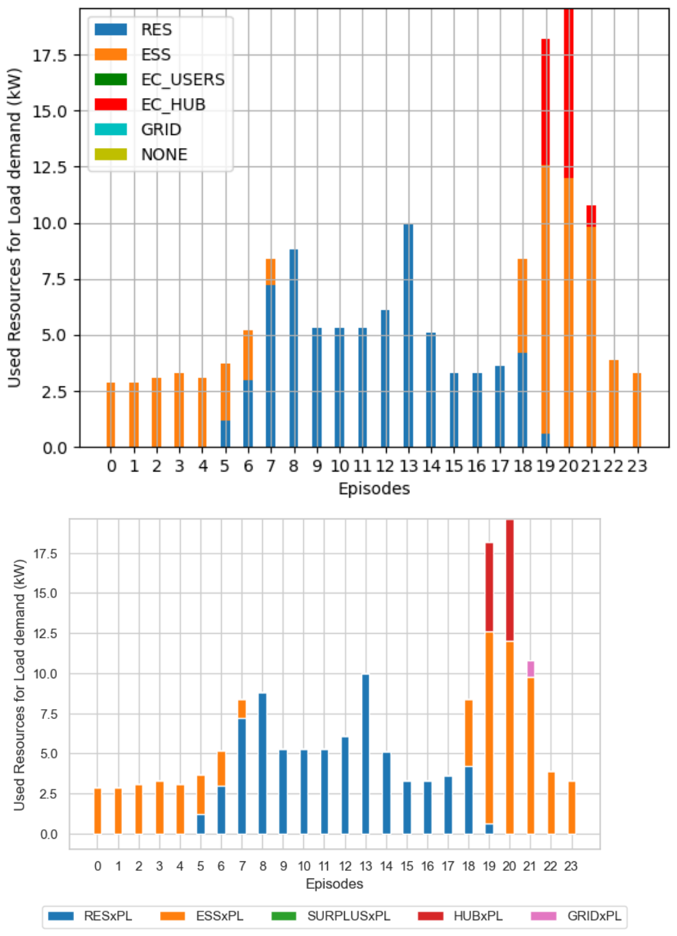
Table A1.
Comparison between Q-Tabular and DQN load power exchanged.
Figure A2.
Q-Tabular vs. DQN—ESS recharge power exchanged (top: Q-Tabular; bottom: DQN).
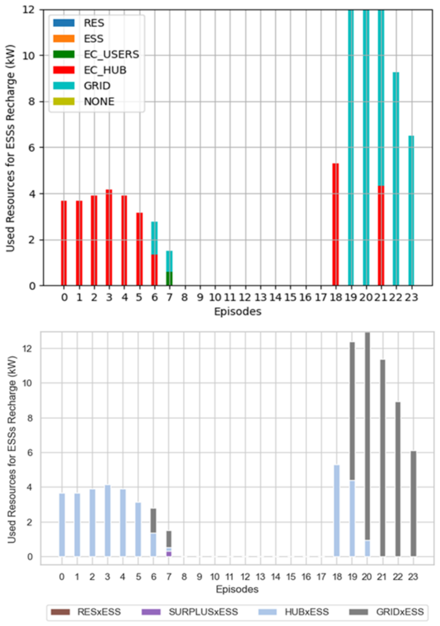
The Q-Tabular implementation had been developed using three sequential stages for respectively load demand satisfaction (stage 1), ESS recharge management (stage 2), and renewable energy surplus selling (stage 3). Stage 3 includes the recharge of the HUB that cannot be performed before the termination of the previous stages. The DQN solution does not use sequential stages and, thus, allows the concurrent execution of ESS recharge, HUB recharge and the selling of the community renewable energy.
The differences between the two plots are only related to the time slots 7 and 19–23, and are caused by the elimination of the 3-stages approach and the functional evolution of the use of the HUB implemented in the DQN solution. In particular, in time slot 7, DQN solution enables the HUB recharge using the community renewable energy and, thus, the HUB returns available to recharge ESSs, while, as in the Q-Tabular solution, the HUB remains unavailable and the ESSs recharge is performed only using the community renewable energy and the Grid.
Table A2 numerically confirms the above considerations and outlines minor differences in the use of both the HUB and the GRID in time slots 19–23. It is worth pointing out that the daily cumulative power used for the ESS recharging in Q-Tabular implementation is equal to 83.82 kW and is the same for the DQN implementation; the punctual differences in HUB and GRID values only depend on the different use of the HUB, as explained above.
Table A2.
Comparison between Q-Tabular and DQN ESS recharge power exchanged.
Figure A3 shows the power exchanged, associated with community renewable energy exchanged to recharge the HUB and to be sold to the Grid. Only time slot 7 is different, as HUB has been used for ESS recharge in DQN control framework with respect to the Q-learning algorithm, where the Grid has been used to recharge the ESSs. Table A3 numerically confirms the above considerations.
Figure A3.
Q-Tabular vs. DQN—power selling (top: Q-Tabular; bottom: DQN).
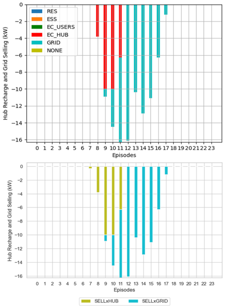
Table A3.
Comparison between Q-Tabular and DQN power selling.
Finally, Figure A4 shows the comparison between the Q-Tabular resource schedule (top) and the DQN resource schedule (bottom).
Figure A4.
Resources schedule (top: Q-Tabular; bottom: DQN).
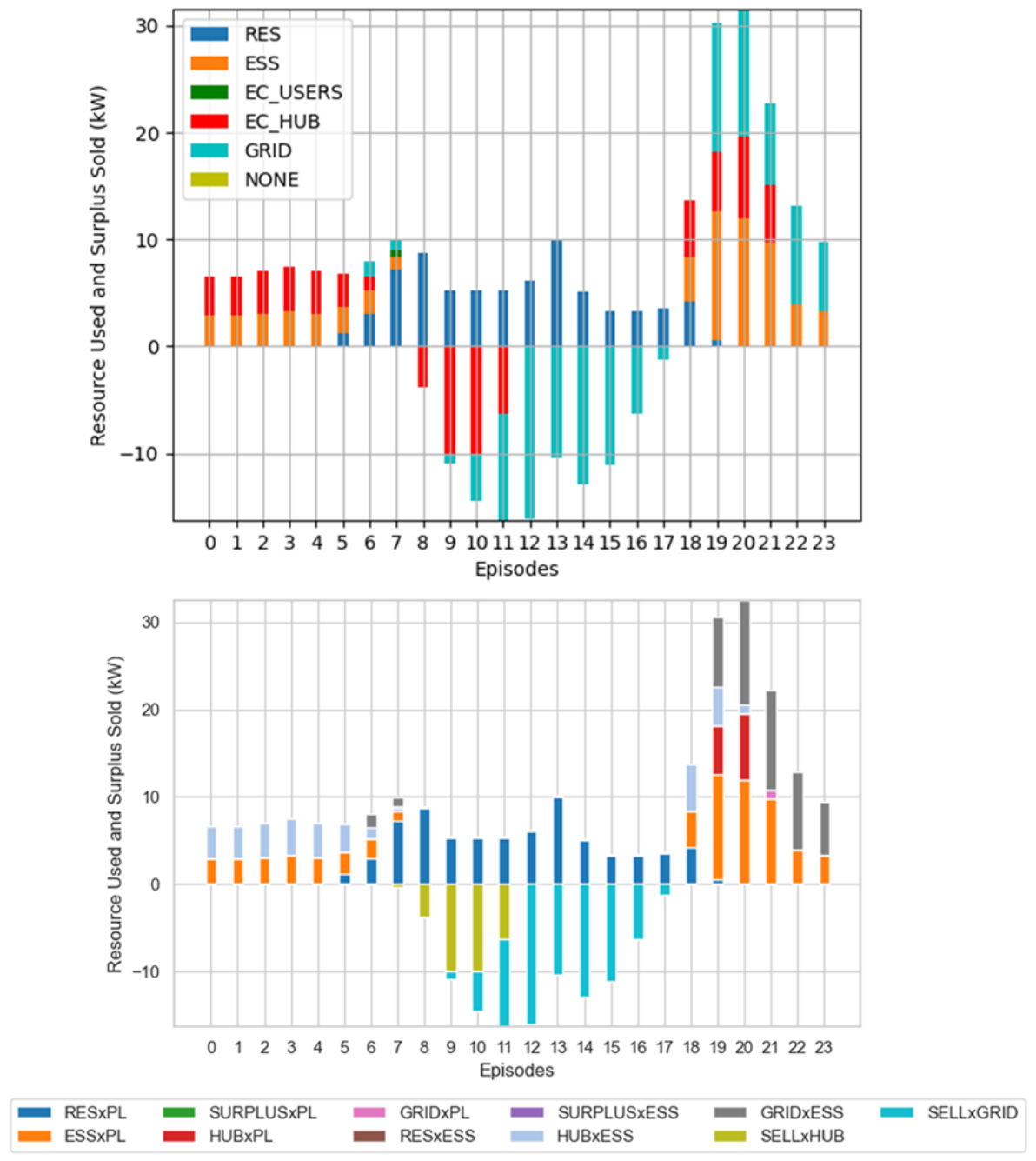
The two plots always show identical use of the resources apart from the time slots 7 and 19–21. The causes of these differences are already provided in the descriptions related to Figure A1, Figure A2 and Figure A3.
With regard to the training time, the DQN solution design of the learning process has been improved using one generic agent representative of all the energy community agents. The trained agent has been instantiated a number of times equal to the number of EC customers during the validation process. In contrast, the Q-Tabular implementation has foreseen the training of all the energy community agents.
Table A4 reports the training times of both solutions under different EC configurations, and outlines that the DQN training time is constant and less than the Q-Tabular one—also in the EC configuration with six customers.
Table A4.
Training execution times.
References
- Battula, A.R.; Vuddanti, S.; Salkuti, S. Review of Energy Management System Approaches in Microgrids. Energies 2021, 14, 5459. [Google Scholar] [CrossRef] [Scilit]
- Shakeri, M.; Pasupuleti, J.; Amin, N.; Rokonuzzaman, M.; Low, F.W.; Yaw, C.T.; Asim, N.; Samsudin, N.A.; Tiong, S.K.; Hen, C.K.; et al. An Overview of the Building Energy Management System Considering the Demand Response Programs, Smart Strategies and Smart Grid. Energies 2020, 13, 3299. [Google Scholar] [CrossRef] [Scilit]
- Etedadi, F.A.; Agbossou, K.; Kelouwani, S.; Henao, N.; Hosseini, S.S. Coordination of Smart Home Energy Management Systems in Neighborhood Areas: A Systematic Review. IEEE Access 2021, 9, 36417–36443. [Google Scholar] [CrossRef] [Scilit]
- Gomes, I.; Bot, K.; Ruano, M.G.; Ruano, A. Recent Techniques Used in Home Energy Management Systems: A Review. Energies 2022, 15, 2866. [Google Scholar] [CrossRef] [Scilit]
- Han, B.; Zahraoui, Y.; Mubin, M.; Mekhilef, S.; Seyedmahmoudian, M.; Stojcevski, A. Home Energy Management Systems: A Review of the Concept, Architecture, and Scheduling Strategies. IEEE Access 2023, 11, 19999–20025. [Google Scholar] [CrossRef] [Scilit]
- Crowley, B.; Kazempour, J.; Mitridati, L.; Alizadeh, M. Learning prosumer behavior in energy communities: Integrating bilevel programming and online learning. Appl. Energy 2025, 392, 125932. [Google Scholar] [CrossRef] [Scilit]
- European Commission. Greenhouse Gas Emissions from Energy Use in Buildings in Europe; European Commission: Brussels, Belgium, 2025.
- European Commission. Directorate-General for Climate Action (European Commission)—Going Climate-Neutral by 2050: A Strategic Long Term Vision for a Prosperous, Modern, Competitive and Climate Neutral EU Economy; European Commission: Brussels, Belgium, 2019.
- European Parliament and Council. Directive (EU) 2018/2001 of the European Parliament and of the Council—Of 11 December 2018—On the Promotion of the Use of Energy from Renewable Sources; European Parliament and Council: Brussels, Belgium, 2018. [Google Scholar]
- European Parliament and Council. Directive (EU) 2019/944 of the European Parliament and of the Council—On Common Rules for the Internal Market for Electricity and Amending Directive 2012–27 EU; European Parliament and Council: Brussels, Belgium, 2019. [Google Scholar]
- European Parliament and Council. Regulation (EU) 2019/943 on the Internal Market for Electricity; European Parliament and Council: Brussels, Belgium, 2019. [Google Scholar]
- European Parliament and Council. Directive (EU) 2024/1275 of the European Parliament and of the Council of 24 April 2024 on the Energy Performance of Buildings (Recast); European Parliament and Council: Brussels, Belgium, 2024. [Google Scholar]
- Marchetti, B.; Vitali, M.; Biancini, G. Renewable Energy Proliferation and the New Local Energy Community Paradigm: Analysis of a Case Study in Italy. Energies 2024, 17, 1599. [Google Scholar] [CrossRef] [Scilit]
- Neij, L.; Palm, J.; Busch, H.; Bauwens, T.; Becker, S.; Bergek, A.; Buzogany, A.; Candelise, C.; Coenen, F.; Devine Wright, P.; et al. Energy communities lessons learnt, challenges, and policy recommendations. Oxf. Open Energy 2025, 4, oiaf002. [Google Scholar] [CrossRef] [Scilit]
- Janev, V.; Berbakov, L.; Tomasevic, N.; Sotoca, J.M.B.; Lujan, S. Validating the Smart Grid Architecture Model for Sustainable Energy Community Implementation: Challenges, Solutions, and Lessons Learned. Energies 2025, 18, 641. [Google Scholar] [CrossRef] [Scilit]
- Vernay, A.L.; Sebi, C.; Arroyo, F. Energy community business models and their impact on the energy transition: Lessons learnt from France. Energy Policy 2023, 175, 113473. [Google Scholar] [CrossRef] [Scilit]
- Hernandez-Matheus, A.; Loschenbrand, M.; Berg, K.; Fuchs, I.; Aragues-Penalba, M.; Bullich-Massaguè, E.; Sumper, A. A systematic review of machine learning techniques related to local energy communities. Renew. Sustain. Energy Rev. 2022, 170, 112651. [Google Scholar] [CrossRef] [Scilit]
- Kandpal, B.; Backe, S.; Crespo del Granado, P. Enhancing bargaining power for energy communities in renewable power purchase agreements using Gaussian learning and fixed price bargaining. Energy 2024, 309, 133016. [Google Scholar] [CrossRef] [Scilit]
- Marchetti, B.; Castelli, G.; Corvaro, F. The Role of Energy Sharing Mechanisms in Advancing the Sustainable Development Goals Outlined in the 2030 Agenda. Energies 2025, 18, 5761. [Google Scholar] [CrossRef] [Scilit]
- Lucas, A.; Carvalhosa, S. Renewable Energy Community Pairing Methodology Using Statistical Learning Applied to Georeferenced Energy Profiles. Energies 2022, 15, 4789. [Google Scholar] [CrossRef] [Scilit]
- Di Nucci, M.R.; Krug, M.; Schwarz, L.; Gatta, V.; Laes, E. Learning from Other Community Renewable Energy Projects: Transnational Transfer of Multi Functional Energy Gardens from the Netherlands to Germany. Energies 2023, 16, 3270. [Google Scholar] [CrossRef] [Scilit]
- Dogan, F.; Oyucu, S.; Unsal, D.B.; Aksoz, A.; Vafaeipour, M. Impact of Environmental Conditions on Renewable Energy Prediction: An Investigation Through Tree Based Community Learning. Appl. Sci. 2025, 15, 336. [Google Scholar] [CrossRef] [Scilit]
- Alam, M.M.; Jang, Y.M. Deep learning based optimal energy management framework for community energy storage system. ICT Express 2023, 9, 333–340. [Google Scholar] [CrossRef] [Scilit]
- Alam, M.M.; Bin Mofidul, R.; Jang, Y.M. Community energy storage system: Deep learning based optimal energy management solution for residential community. J. Energy Storage 2023, 64, 107100. [Google Scholar] [CrossRef] [Scilit]
- Cicceri, G.; Tricomi, G.; D’Agati, L.; Longo, F.; Merlino, G.; Puliafito, A. A Deep Learning-Driven Self-Conscious Distributed Cyber-Physical System for Renewable Energy Communities. Sensors 2023, 23, 4549. [Google Scholar] [CrossRef] [Scilit]
- Khan, M.; Faisal, M.; Albogamy, F.; Diyan, M. Deep Learning and Heuristic Optimization for Secure and Efficient Energy Management in Smart Communities. Comput. Model. Eng. Sci. 2025, 143, 2027–2052. [Google Scholar] [CrossRef] [Scilit]
- Giannuzzo, L.; Minuto, F.D.; Schiera, D.S.; Lanzini, A. Reconstructing hourly residential electrical load profiles for Renewable Energy Communities using non intrusive machine learning techniques. Energy AI 2024, 15, 100329. [Google Scholar] [CrossRef] [Scilit]
- Elomari, Y.; Mateu, C.; Marin Genesca, M.; Boer, D. A data driven framework for designing a renewable energy community based on the integration of machine learning model with life cycle assessment and life cycle cost parameters. Appl. Energy 2024, 358, 122619. [Google Scholar] [CrossRef] [Scilit]
- Mo, M.; Xiong, X.; Wu, Y.; Yu, Z. Deep-Reinforcement-Learning-Based Low-Carbon Economic Dispatch for Community-Integrated Energy System under Multiple Uncertainties. Energies 2023, 16, 7669. [Google Scholar] [CrossRef] [Scilit]
- Li, P.; Gu, C.; Cheng, X.; Li, J.; Alhazmi, M. Integrated energy-water systems for community-level flexibility: A hybrid deep Q-network and multi-objective optimization framework. Energy Rep. 2025, 13, 4813–4826. [Google Scholar] [CrossRef] [Scilit]
- Salazar Duque, E.M.; Giraldo, J.S.; Vergara, P.P.; Nguyen, P.; van der Molen, A.; Slootweg, H. Community energy storage operation via reinforcement learning with eligibility traces. Electr. Power Syst. Res. 2022, 212, 108515. [Google Scholar] [CrossRef] [Scilit]
- Liu, C.; Xue, Z. Adaptive Optimization Design of Building Energy System for Smart Elderly Care Community Based on Deep Deterministic Policy Gradient. Processes 2023, 11, 2155. [Google Scholar] [CrossRef] [Scilit]
- Vetter, V.; Wohlgenannt, P.; Kepplinger, P.; Eder, E. Deep Reinforcement Learning Approaches the MILP Optimum of a Multi-Energy Optimization in Energy Communities. Energies 2025, 18, 4489. [Google Scholar] [CrossRef] [Scilit]
- Dolatabadi, M.; Zakariazadeh, A.; Borghetti, A.; Siano, P. Distributed Energy and Reserve Scheduling in Local Energy Communities Using L-BFGS Optimization. CSEE J. Power Energy Syst. 2024, 10, 942–952. [Google Scholar] [CrossRef] [Scilit]
- Tortorelli, A.; Sabina, G.; Marchetti, B. A Cooperative Multi-Agent Q-Learning Control Framework for Real-Time Energy Management in Energy Communities. Energies 2024, 17, 5199. [Google Scholar] [CrossRef] [Scilit]
- Tostado-Veliz, M.; Giraldo, J.S.; Icaza Álvarez, D.; Cruz, C.; Jurado, F. Robust day-ahead scheduling of cooperative energy communities considering multiple aggregators. Sustain. Cities Soc. 2024, 116, 105878. [Google Scholar] [CrossRef] [Scilit]
- Berg, K.; Rana, R.; Farahmand, H. Quantifying the benefits of shared battery in a DSO-energy community cooperation. Appl. Energy 2023, 343, 121105. [Google Scholar] [CrossRef] [Scilit]
- Xie, Y.; Yao, Y.; Wang, Y.; Cha, W.; Zhou, S.; Wu, Y.; Huang, C. A Cooperative Game-Based Sizing and Configuration of Community-Shared Energy Storage. Energies 2022, 15, 8626. [Google Scholar] [CrossRef] [Scilit]
- Choucair, Z.; Zaibidi, N.Z.; Ahmad, N. Fuzzy Cooperative Games with Coalition Values Based on Gaussian Fuzzy Numbers and Their Application to Energy Sharing in Residential Communities. Int. J. Fuzzy Syst. 2025, 28, 905–919. [Google Scholar] [CrossRef] [Scilit]
- Lilliu, F.; Reforgiato Recupero, D. A cooperative game-theory approach for incentive systems in local energy communities. Sustain. Energy Grids Netw. 2024, 38, 101391. [Google Scholar] [CrossRef] [Scilit]
- Abedrabboh, K.; Al-Fagih, L.; Parilina, E.; Sedakov, A. Incentivising community self-consumption in energy markets: Stable coalition formation using cooperative game theory. Appl. Energy 2025, 399, 126508. [Google Scholar] [CrossRef] [Scilit]
- Toderean, L.; Chifu, V.R.; Cioara, T.; Anghel, I.; Pop, C.B. Cooperative Games Over Blockchain and Smart Contracts for Self-Sufficient Energy Communities. IEEE Access 2023, 11, 73982–73999. [Google Scholar] [CrossRef] [Scilit]
- Mitrea, D.; Cioara, T.; Anghel, I.; Toderean, L. Evolutionary game for incentivizing social cooperation of prosumers in transactive energy communities. Energy Build. 2025, 327, 115057. [Google Scholar] [CrossRef] [Scilit]
- Mignoni, N.; Carli, R.; Dotoli, M. Distributed Noncooperative MPC for Energy Scheduling of Charging and Trading Electric Vehicles in Energy Communities. IEEE Trans. Control Syst. Technol. 2023, 31, 2159–2172. [Google Scholar] [CrossRef] [Scilit]
- Kong, W.; Sun, K.; Zhao, J. Two-stage Optimal Scheduling of Community Integrated Energy System Considering Operation Sequences of Hydrogen Energy Storage Systems. J. Mod. Power Syst. Clean Energy 2025, 13, 276–288. [Google Scholar] [CrossRef] [Scilit]
- Ye, Z.; Huang, W.; Huang, J.; He, J.; Li, C.; Feng, Y. Optimal Scheduling of Integrated Community Energy Systems Based on Twin Data Considering Equipment Efficiency Correction Models. Energies 2023, 16, 1360. [Google Scholar] [CrossRef] [Scilit]
- Zhang, W.; Wu, J. A Stochastic MPC-Based Flexibility Scheduling Strategy for Community Integrated Energy System Considering Multi-Temporal-Spatial-Scale and Inertia Components. Processes 2024, 12, 457. [Google Scholar] [CrossRef] [Scilit]
- Yang, M.; Wang, Y.; Wang, J.; Liu, D.; Xu, W. Optimal Scheduling of Integrated Energy Systems in Low-Carbon Communities Considering Flexibility of Resources and Segmental Control of Solid Oxide Fuel Cells. J. Mod. Power Syst. Clean Energy 2025, 13, 915–927. [Google Scholar] [CrossRef] [Scilit]
- He, P.; Zhou, L.; Wang, J.; Yang, Z.; Lv, G.; Cai, C.; Zou, H. Optimizing the Operation of Local Energy Communities Based on Two-Stage Scheduling. Processes 2025, 13, 2449. [Google Scholar] [CrossRef] [Scilit]
- Dinh, H.T.; Kim, D.; Kim, D. MILP-based optimal day-ahead scheduling for system-centric CEMS supporting different types of homes and energy trading. arXiv 2022, arXiv:2202.10181. [Google Scholar] [CrossRef] [Scilit]
- Foroozandeh, Z.; Limmer, S.; Lezama, F.; Faia, R.; Ramos, S.; Soares, J. A MBNLP Method for Centralized Energy Pricing and Scheduling in Local Energy Community. In Proceedings of the 2022 IEEE PES Generation, Transmission and Distribution Conference and Exposition—Latin America (IEEE PES GTD Latin America); IEEE: New York, NY, USA, 2022; pp. 1–6. [Google Scholar] [CrossRef] [Scilit]
- Lilla, S.; Orozco, C.; Borghetti, A.; Napolitano, F.; Tossani, F. Day-Ahead Scheduling of a Local Energy Community: An Alternating Direction Method of Multipliers Approach. IEEE Trans. Power Syst. 2020, 35, 1132–1142. [Google Scholar] [CrossRef] [Scilit]
- Cornélusse, B.; Savelli, I.; Paoletti, S.; Giannitrapani, A.; Vicino, A. A community microgrid architecture with an internal local market. Appl. Energy 2019, 242, 547–560. [Google Scholar] [CrossRef] [Scilit]
- Capper, T.; Gorbatcheva, A.; Mustafa, M.A.; Bahloul, M.; Schwidtal, J.M.; Chitchyan, R.; Andoni, M.; Robu, V.; Montakhabi, M.; Scott, I.J.; et al. Peer-to-peer, community self-consumption, and transactive energy: A systematic literature review of local energy market models. Renew. Sustain. Energy Rev. 2022, 162, 112403. [Google Scholar] [CrossRef] [Scilit]
- Dynge, M.; Berg, K.; Bjarghov, S.; Cali, U. Local electricity market pricing mechanisms’ impact on welfare distribution, privacy and transparency. Appl. Energy 2023, 341, 121112. [Google Scholar] [CrossRef] [Scilit]
- Balegamire, R.; Gautier, A. Pricing and sharing rules for energy communities. Util. Policy 2025, 96, 101995. [Google Scholar] [CrossRef] [Scilit]
- Ba, J.L.; Kiros, J.R.; Hinton, G.E. Layer Normalization. arXiv 2016, arXiv:1607.06450. [Google Scholar] [CrossRef] [Scilit]
- European Commission. Special Eurobarometer 527—Report—Fairness Perceptions of the Green Transition—Fieldwork: May–June 2022; European Commission: Brussels, Belgium, 2022.
- Kingma, D.P.; Ba, J. Adam: A Method for Stochastic Optimization. arXiv 2017, arXiv:1412.6980. [Google Scholar]
- Mean Squared Error, 2025. Wikipedia—Page Version ID: 1316575636. Available online: https://en.wikipedia.org/wiki/Mean_squared_error (accessed on 1 October 2026).
- European Commission. Photovoltaic Geographical Information System (PVGIS); European Commission: Brussels, Belgium, 2026.
- Farebrother, J.; Machado, M.C.; Bowling, M. Generalization and Regularization in DQN. arXiv 2020, arXiv:1810.00123. [Google Scholar] [CrossRef] [Scilit]
- Madhyastha, P.; Jain, R. On Model Stability as a Function of Random Seed. arXiv 2019, arXiv:1909.10447. [Google Scholar] [CrossRef] [Scilit]
- GSE. Available online: https://www.gse.it/en/ (accessed on 1 October 2026).
- ARERA. Available online: https://www.arera.it/ (accessed on 1 October 2026).
- European Parliament and Council. Regulation (EU) 2017/2195 on Guideline on Electricity Balancing; European Parliament and Council: Brussels, Belgium, 2017. [Google Scholar]
- Watkins, C.; Dayan, P. Q-Learning. Mach. Learn. 1992, 8, 279–292. [Google Scholar] [CrossRef] [Scilit]
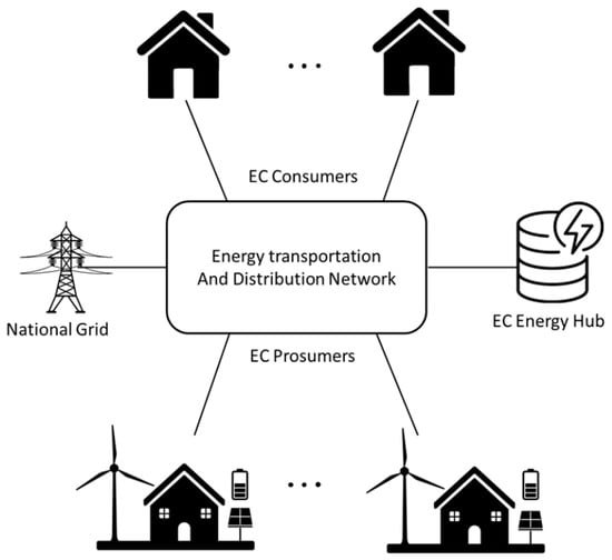
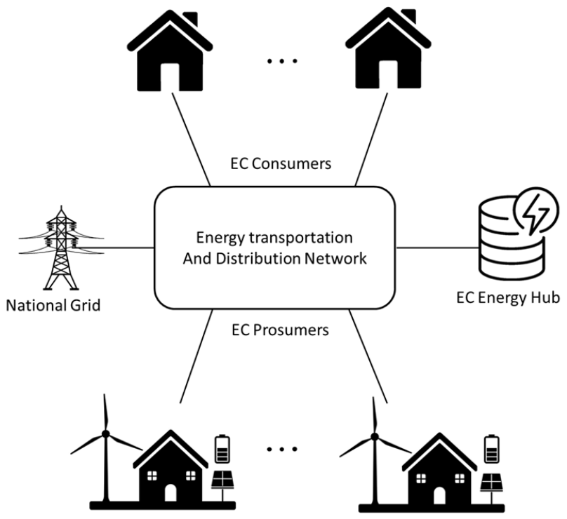
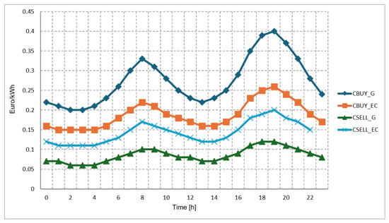
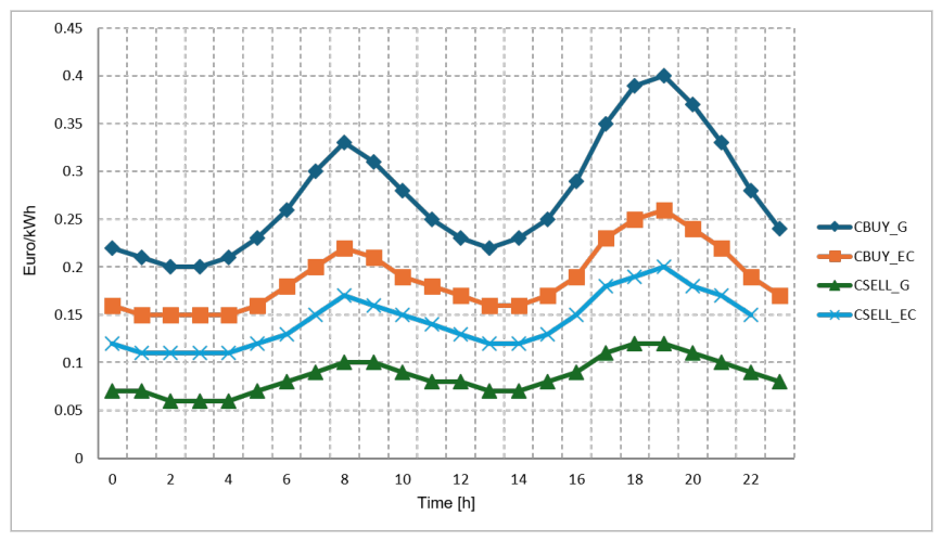
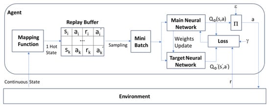
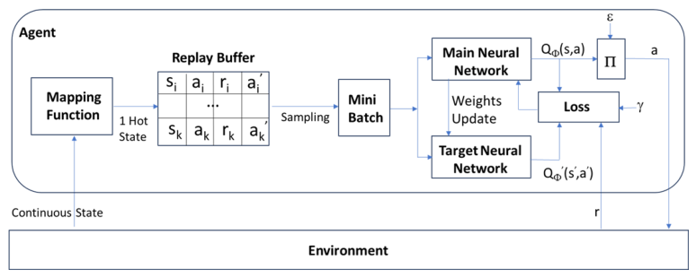
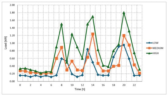
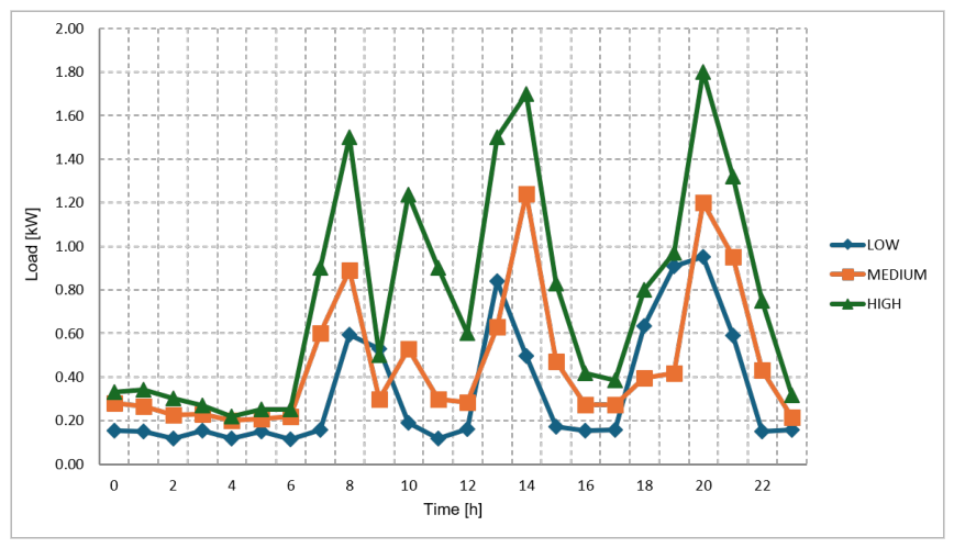
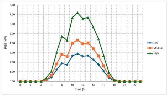
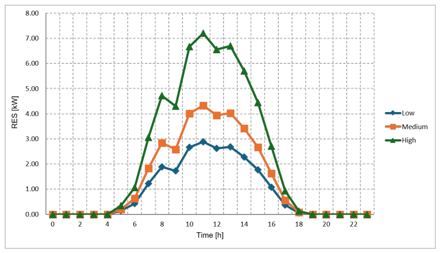
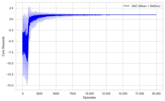
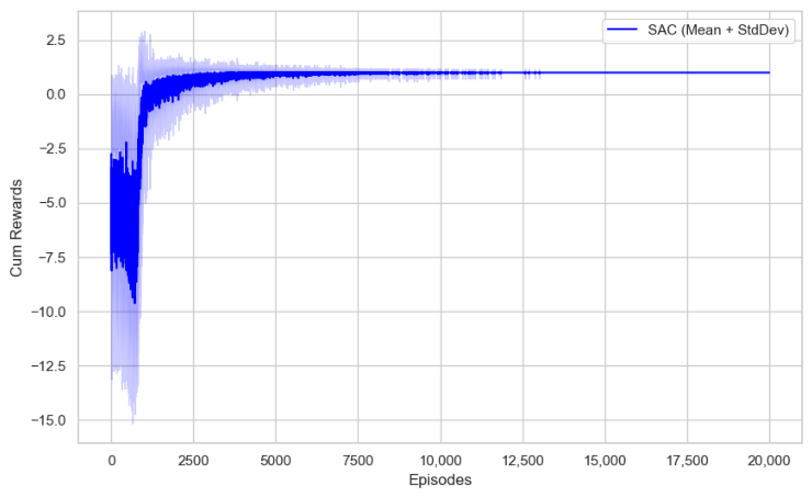
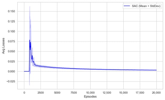
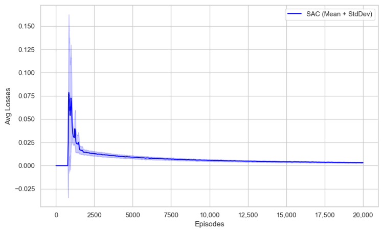
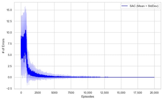
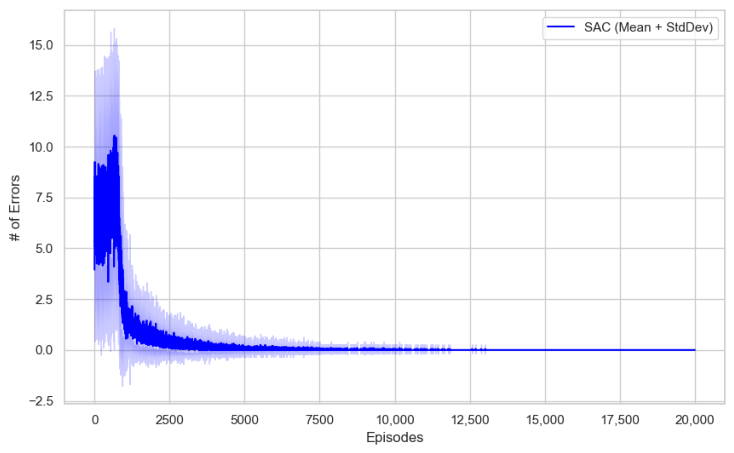
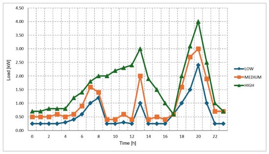
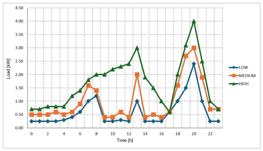
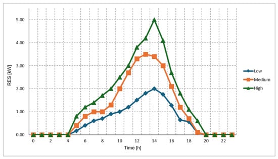
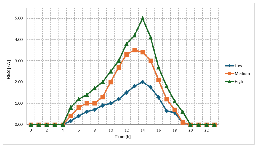
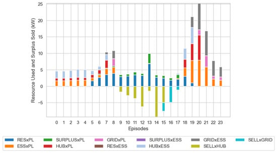
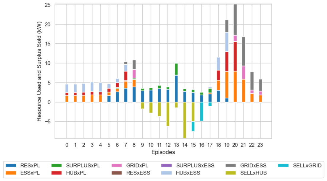
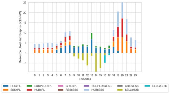
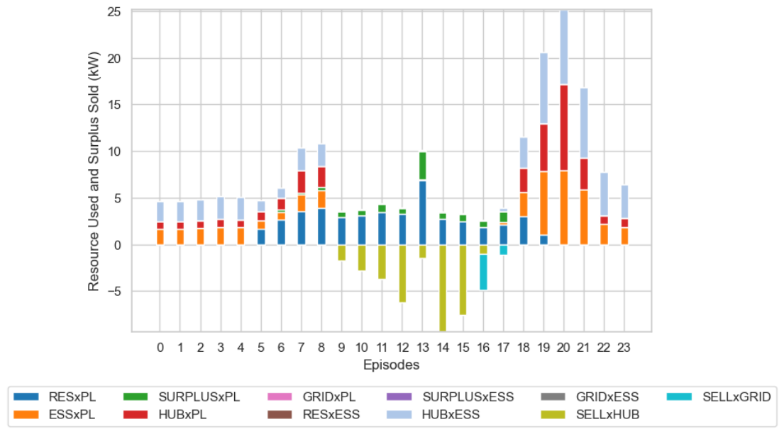
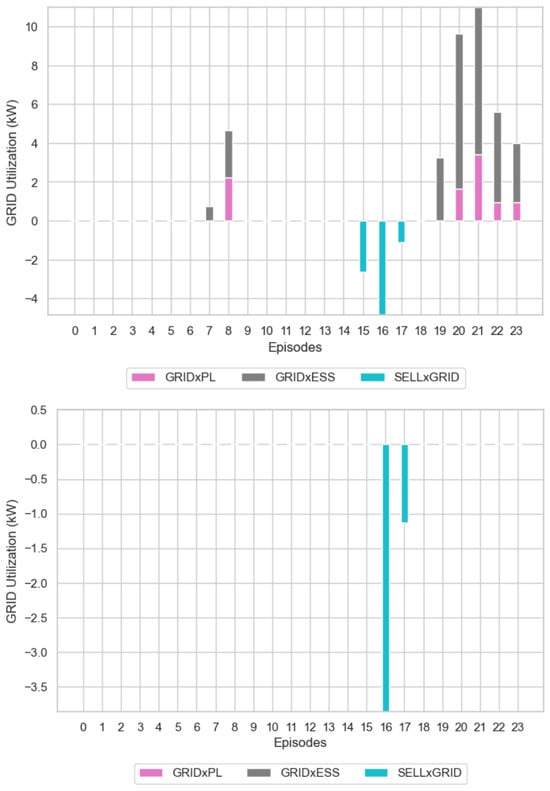
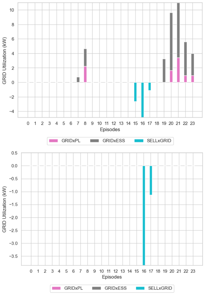
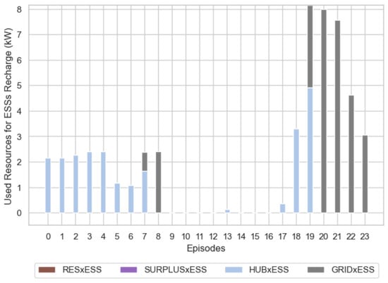
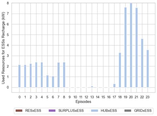
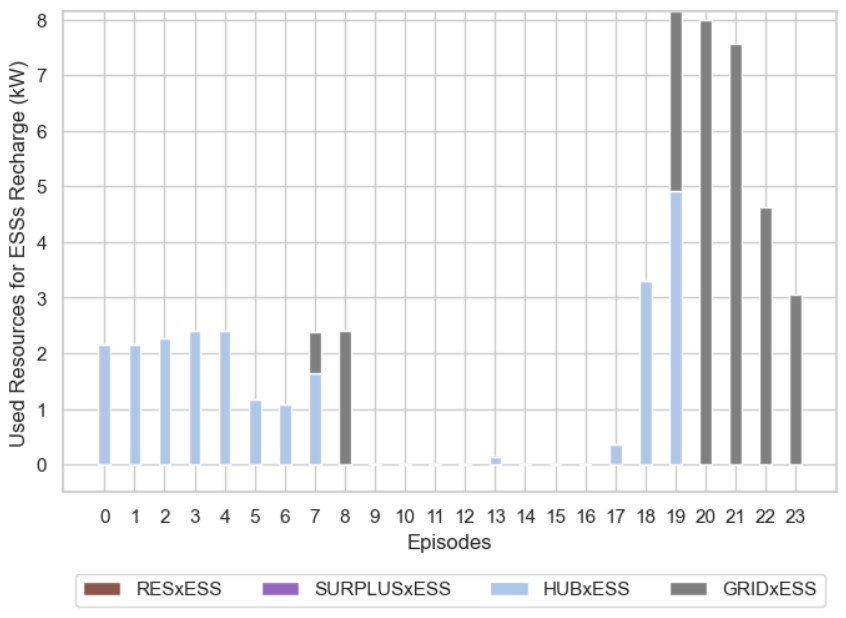
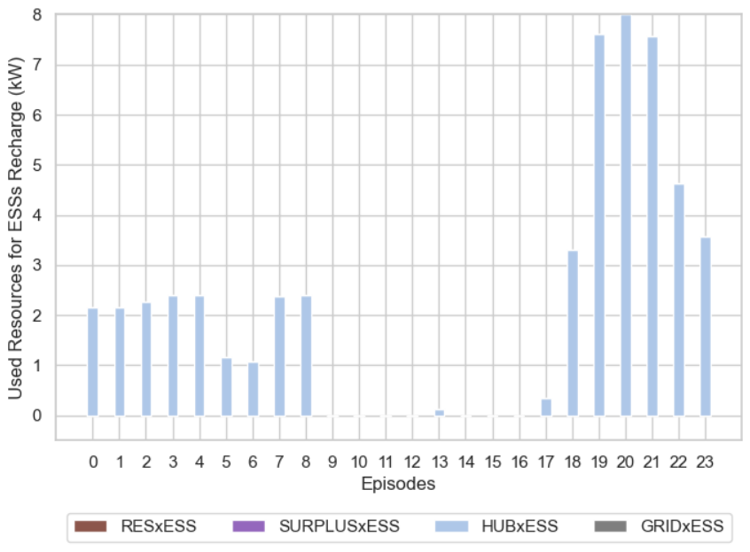
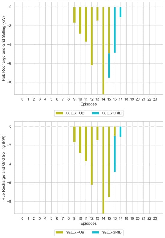
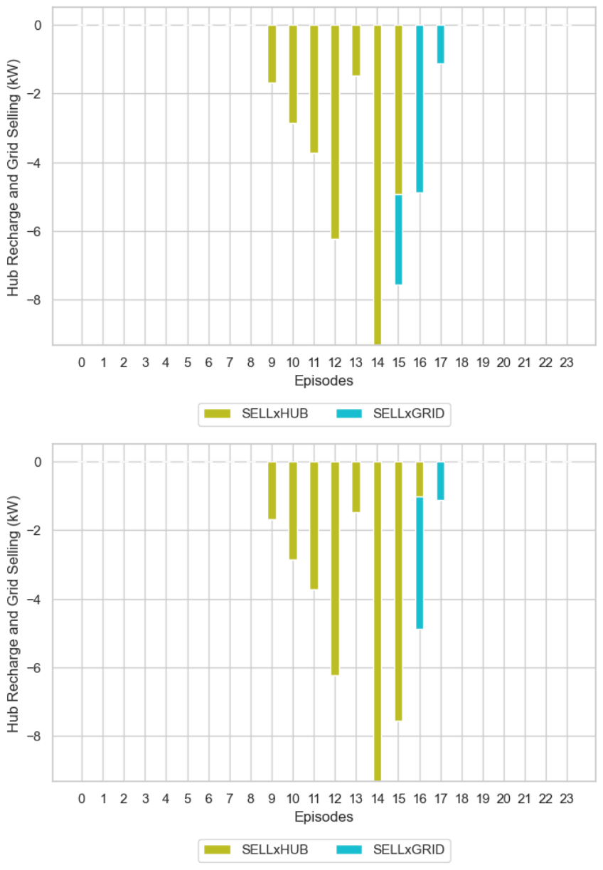
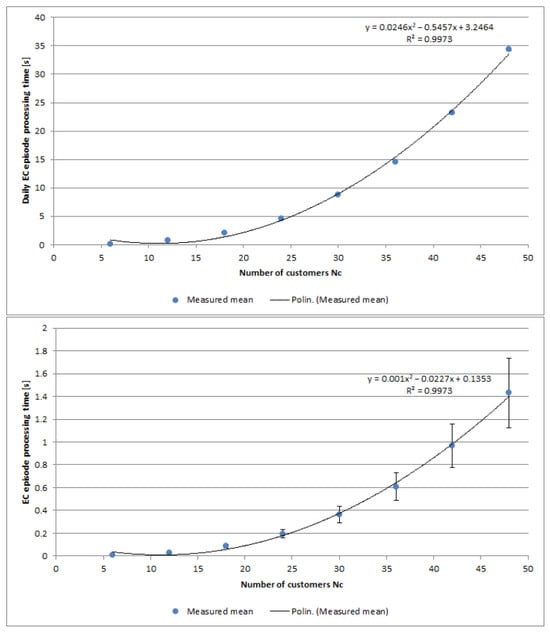
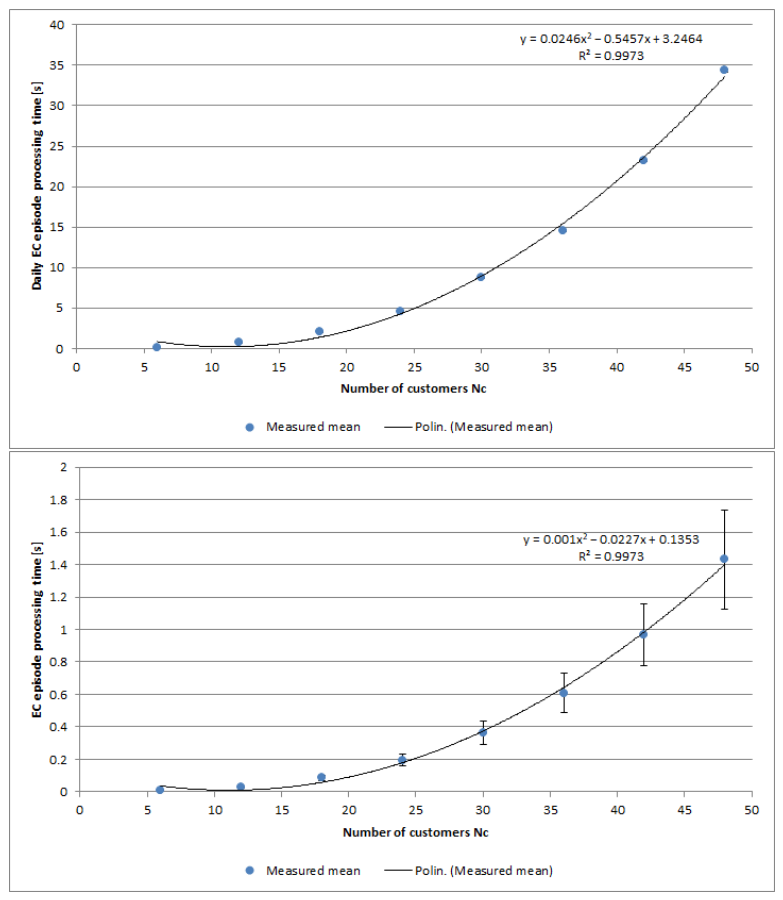
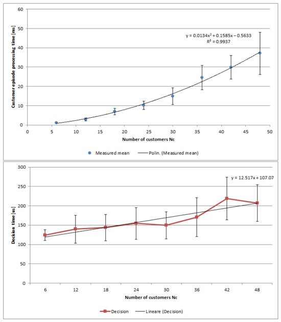
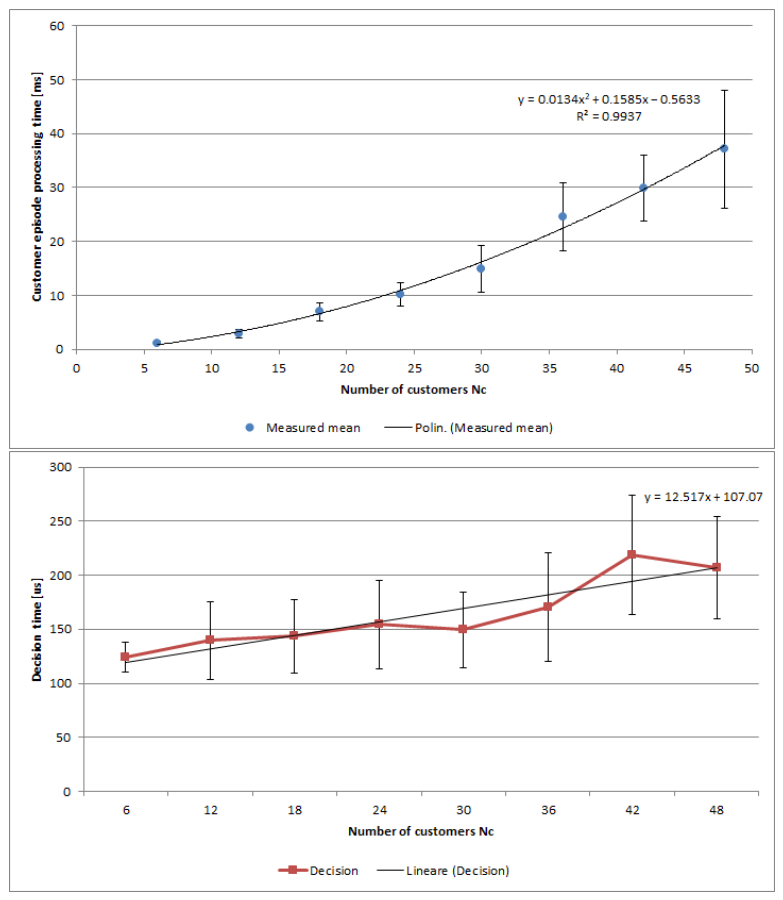
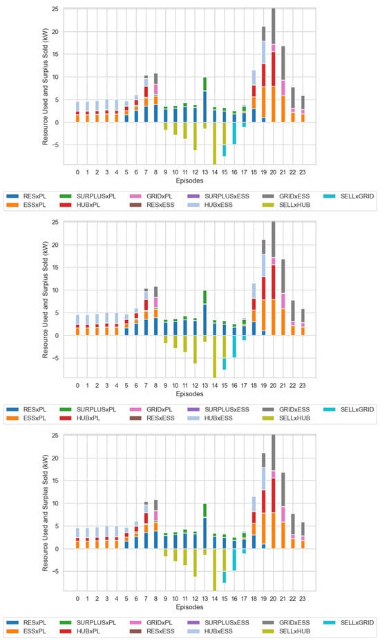
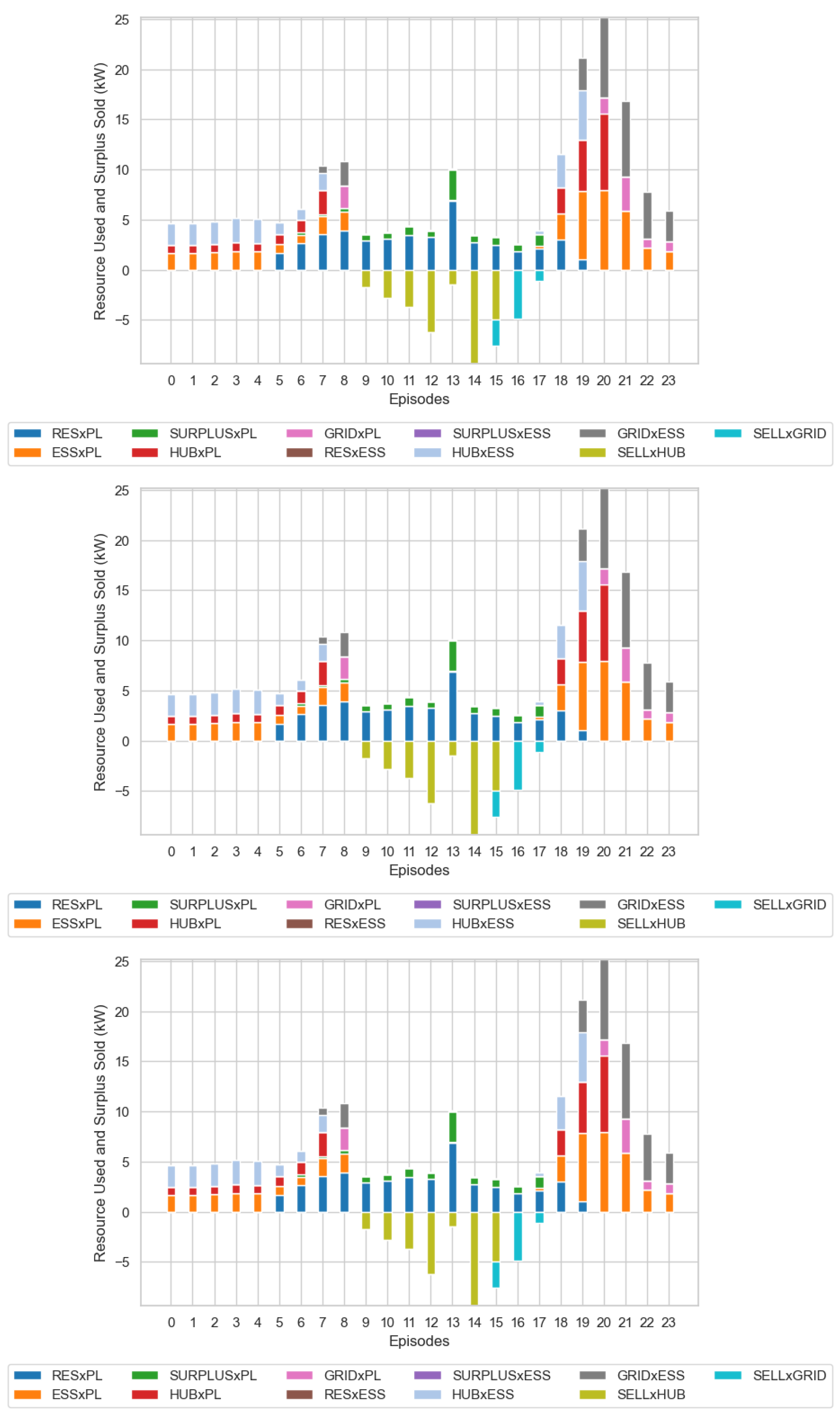

Disclaimer/Publisher’s Note: The statements, opinions and data contained in all publications are solely those of the individual author(s) and contributor(s) and not of MDPI and/or the editor(s). MDPI and/or the editor(s) disclaim responsibility for any injury to people or property resulting from any ideas, methods, instructions or products referred to in the content. |
© 2026 by the authors. Licensee MDPI, Basel, Switzerland. This article is an open access article distributed under the terms and conditions of the Creative Commons Attribution (CC BY) license.