


Abstract
Forecast calibration changes battery schedules, but its economic effect depends on how planned actions are executed. We cross two residual calibrations of photovoltaic (PV) and load forecasts with a charging-only feedback rule in hourly receding-horizon scheduling with five- or fifteen-minute execution. Environment A combines modeled PERFORM PV with scaled ERCOT Coast demand; B and C are metered CoSSMic households. Three environments, three forecast treatments, three feedback intensities, and three tariff scenarios give 81 configurations, 18 of which duplicate uncalibrated cells because validation selected zero weighted-mean gain for B and C. Median calibration lowers A’s first-step net-load mean absolute error by 8.47% yet raises its cost, whereas in B and C it increases the error by 0.695% and 0.629%. Under the reference tariff, the calibration-by-feedback interaction is −3622.9 currency units (CU) (−0.251%) in A, where the more accurate forecast costs more, and CU −0.279 (−0.088%) and CU −0.371 (−0.117%) in B and C, where feedback attenuates the cost of a worse correction. Identical charging requests can yield different actions because state-of-charge histories differ. Doubling storage in C reverses the interaction to CU +0.370 (+0.124%); A’s flat price interaction, CU +338 (+0.021%), has an interval that includes zero. Findings are conditional on hypothetical tariffs, reconstructed loads, and a restricted feedback rule.
1. Introduction
Photovoltaic (PV) forecasts inform when a battery retains, absorbs, or releases energy, but a forecast changes a bill only through the actions that are executed. Whether a planned action changes a realized transaction depends on execution permissions, information latency, stored energy, and prices. Forecast-informed economic model predictive control (MPC) is established in practice. Kull et al. implemented linear economic MPC for microgrid dispatch on field-ready hardware and, in two hardware-in-the-loop scenarios, achieved 72.2–85.5% of the cost savings that perfect foresight would have provided relative to an uncontrolled benchmark; the shortfall reflects imperfect forecasts, hardware implementation, and power fluctuations together [1]. Integrated frameworks couple forecasting with MPC for cost-optimized solar–battery energy management [2]. We examine what happens to operating cost when forecast information and execution permissions change together.
Forecasting research offers several ways to change the information a scheduler receives. Post-processing corrects the output of an existing model; Quan et al., for example, train a deep network in two stages to correct solar forecasts [3]. Ensemble weather prediction supplies a spread of PV scenarios whose added value can be assessed against a single deterministic run [4]. Distributional models, such as conditional variational autoencoders with mixed continuous–discrete outputs [5] and monotonic quantile convolutional networks [6], describe forecast uncertainty directly, and simple estimators can provide forecast error magnitudes quickly [7]. Each approach changes a different property of the prediction: its bias, its spread, or the description of its error. The residual calibrations studied here belong to the first group, because they shift point forecasts by recent error statistics. Assessing their operational value requires a feasible action set and a settlement rule, and a reduction in point error must be distinguished from the provision of additional operating reserve.
Forecast skill and economic value are related but not interchangeable. Schmitt et al. found that the operating cost of an MPC-controlled building under peak pricing rises approximately linearly with PV forecast error; the exact relationship depended on how information for the current interval was handled, and only the first 75 min of a 24 h forecast affected cost [8]. Other studies show that skill and value can diverge. In a microgrid with PV, stationary storage, and electric vehicle charging, Manzolini et al. found that a vehicle load forecast with 30% lower root mean square error than persistence, when combined with the PV forecast, increased the combined forecast error by 15% and the operating cost by up to 5% [9]. Campos et al. tested eleven levels of solar forecast accuracy for PV–battery plants in a day-ahead market and found that less accurate forecasts pushed the battery towards price arbitrage and could increase revenue [10]. Fiori Maccioni et al. ranked price-forecasting methods by the battery arbitrage profit they produced rather than by error alone [11]. Further studies attach economic weights to forecast errors through hybrid dispatch [12], schedule deviation penalties [13], and ramp-sensitive intraday operation [14]. Probabilistic information can also change the reserve held: adaptive conformal bounds in rolling-horizon scheduling trade operating cost against state-of-charge exposure [15], whereas Bayesian probabilistic PV forecasts combined with stochastic MPC reduced simulated operating cost by 20–35% relative to an expected value forecast [16]. A cost increase after an accuracy gain is therefore not new; what has received less attention is how such a result changes when the rule that executes the plan is varied.
Execution feedback must be defined by its permitted actions. Zhang et al. compare day-ahead battery scheduling with closed-loop MPC that re-optimizes from measured load and state of charge (SOC) and report that the economic effects of forecast information and feedback are not additive [17]. Two-time-scale scheduling [18], bi-layer MPC [19], and local control of PV–storage units with lightweight probabilistic forecasts [20] assign different measured variables and control responsibilities to each layer. Within-hour correction may also concern reactive power while the active power reference remains fixed [21]. Ma et al. study scenario-based ultra-short-term rolling operation of a PV–storage system under forecast uncertainty and report a trade-off between load-shifting performance and operational risk [22]. Xu et al. formulate a joint forecasting and declaration strategy for oversized PV–storage plants under scenario-oriented uncertainty, with generation and deviation penalties as two objectives, and compare weather conditions, storage capacities, and DC/AC ratios [23]. These precedents motivate tracing a specified intervention through each execution stage from plan to request, physical limit, and stored energy, rather than treating the presence of feedback as a uniform system property.
Physical and economic conditions also determine forecast value. Scheduling with known generation or historical measured inputs supports dispatch analysis [24,25] without establishing the benefit of an attainable forecast improvement. Flexible cooling [26] or uncertain residential and vehicle demand [27] changes the feasible set. Aging-aware sizing and operation [28,29] and degradation-sensitive scheduling [30,31,32] change the value assigned to battery use. Our constant discharged energy charge is a pack-throughput economic proxy; these studies motivate sensitivity analysis but do not validate its coefficient or imply a battery life benefit.
Transferability requires a distinction between sources and scenarios. Transfer learning can reuse forecasting models when target data are limited [33], multi-building studies relate the data used for forecasting to MPC performance [34], household studies vary loads and price years [35], and apartment building studies validate complete forecast–optimization chains [36]. Two households from one acquisition project provide more environmental variation than rescaling one sequence, but they do not establish population-level generalizability. Similarly, transferring a residual window together with terminal valuation tests joint controller settings, not the portability of forecasting alone.
The closest studies differ in which elements they vary. Schmitt et al. vary PV forecast error together with the handling of current-interval information [8], whereas Manzolini et al. [9] and Campos et al. [10] vary forecast quality under a fixed execution rule. Zhang et al. already combine forecast-based scheduling with measured-state feedback and identify non-additive information and feedback effects [17], and Ma et al. [22] and Xu et al. [23] evaluate rolling and declaration-based PV–storage operation under forecast uncertainty. None of these elements is claimed as new here. Supplementary Table S2 compares the eight closest studies in terms of their information and execution structure, environment, and evaluated evidence. The present contribution is narrower: the charging request rule of Equation (4), whose intensity α takes the values 0, 1/2, and 1, is crossed with median and exponentially weighted residual calibration under matched information timing, hardware, and settlement. We ask how this rule changes the marginal cost effect of calibration, and we follow paired forecast-induced plan differences through requests, physical clipping, and accumulated state.
The study makes three contributions. First, a matched 2 × 2 contrast (cells C00–C11 in Figure 1b) measures the calibration-by-execution interaction, and an intermediate intensity, a second calibration, and an alternative selection among near-equivalent schedules test its dependence on these choices. Second, stage-resolved records and common-state diagnostics connect request replacement, clipping, and SOC histories to price-weighted transactions. Third, one protocol is applied to three source environments and three tariff scenarios, and negative, zero, and reversed effects are all reported. The methods are established MPC methods, the findings are conditional on the environments studied, and substitution between calibration and feedback is tested rather than assumed.
Figure 1.
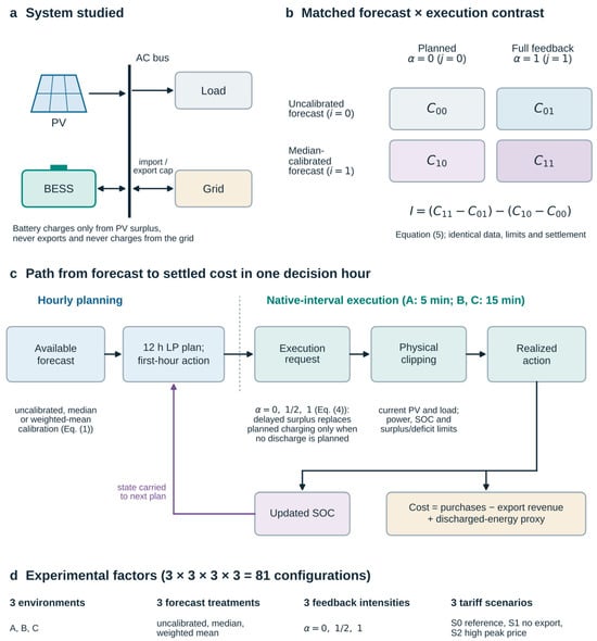
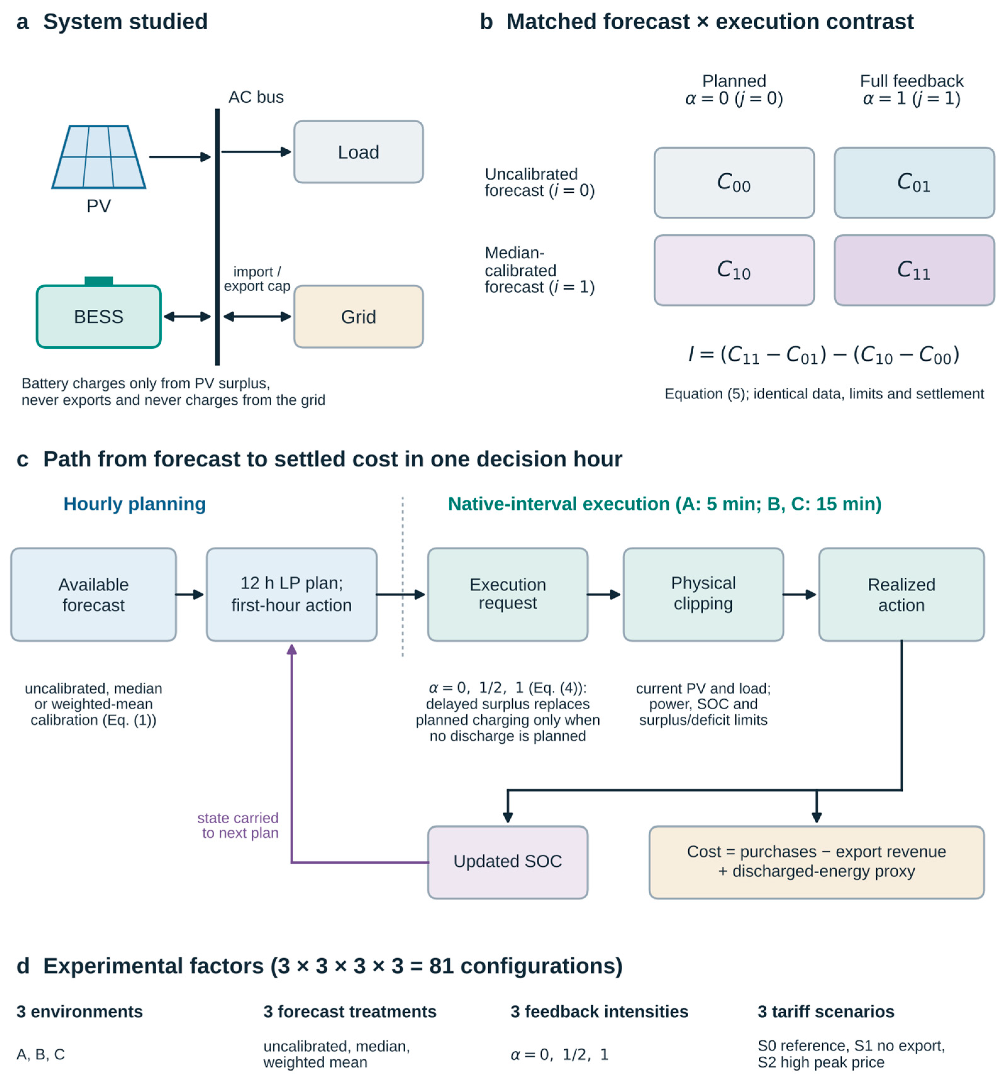
Study design. (a) System: PV, load, BESS, and grid on a common AC bus; the battery charges only from PV surplus and does not export. (b) Matched 2 × 2 contrast; Cij is the realized cost with forecast i (0, uncalibrated; 1, median-calibrated) and execution j (0, planned, α = 0; 1, full feedback, α = 1), and I follows Equation (5). (c) Path from forecast to settled cost within one decision hour; hourly twelve-hour planning feeds five-minute execution in A and fifteen-minute execution in B and C, feedback changes charging requests only when no discharge is planned, and current observations enter physical clipping. (d) Experimental factors of the 81 primary configurations. The diagram represents simulation, not hardware validation.
Figure 1 summarizes the system and the design. Panel (a) shows the system studied: a PV array, an electrical load, and a battery energy storage system (BESS) share an AC bus with the grid. The battery charges only from PV surplus and discharges only to serve load, so it never charges from the grid or exports; the grid supplies deficits and accepts exports up to the cap of the tariff scenario. Panel (b) defines the four cells of the primary contrast: C00 uses the uncalibrated forecast with planned execution, C10 the median-calibrated forecast with planned execution, C01 the uncalibrated forecast with full feedback, and C11 the median-calibrated forecast with full feedback; the interaction I combines them as in Equation (5). Panel (c) traces one decision hour. An hourly linear program (LP) plans twelve hours ahead with the available forecast, and its first-hour action becomes the reference for every native execution interval of that hour. The execution rule may replace the planned charging request with delayed observed surplus; current PV and load, battery power, and stored energy then clip the request to a realizable action. The realized action updates the SOC from which the next hourly plan starts, and the resulting transactions are settled. Panel (d) lists the experimental factors.
2. Materials and Methods
2.1. System, Datasets, and Scenarios
Table 1 summarizes the three environments. Environment A combines model-generated PERFORM PV for site solar433 with ERCOT Coast zonal demand scaled by 0.00025 [37]; it is not a co-located measured installation. Environments B and C are the households residential3 and residential4 of the Open Power System Data (OPSD) household data package, version 2020-04-15, which contains measurements from the CoSSMic project in Konstanz, Germany [38]. For B and C, interval PV and grid power are obtained from differences of cumulative meter readings, load is reconstructed as PV plus imports minus exports, and the one-minute data are aggregated to fifteen-minute execution intervals. Eligibility rules, the chronological training, validation, and test splits, and the treatment of local and UTC time are given in Appendix A.
Table 1.
Dataset and system summary. Step denotes execution resolution; test days count complete eligible UTC days, with the number of episodes (uninterrupted runs of eligible days) in parentheses. A uses PERFORM site solar433 PV and ERCOT Coast demand scaled by 0.00025; B and C are OPSD CoSSMic households. The test period of A is contiguous (275 of 275 calendar days), whereas the test spans of B and C contain gaps. B and C share an acquisition project but use separate household meter profiles.
The training period load peak, P*, sets the scale of each environment. The training PV peak is normalized to 1.5 times this value, the storage energy capacity is 1.5 h times it, and the rated battery power is one quarter of the energy capacity, a four-hour duration (Table 2). These choices define comparable scenarios; they are not recommendations for the original sites. Supplementary Section S1 and Table S1 give the complete constraints, all parameter values, and the basis of each value.
Table 2.
Core system settings. E and P are rated energy and power, and z is fractional SOC, i.e., stored energy divided by the energy capacity; with the energy ratio of 1.5 h, z0 = 0.50 corresponds to s0 = 0.75 h of normalized stored energy. The first two rows are ratios. Values are prespecified modeling assumptions except for the data-derived execution intervals; references support bounded storage and rolling scheduling [1,15,22], not these numerical choices.
Costs are expressed in a generic currency unit (CU). The tariffs are hypothetical and are tied neither to a national currency nor to the original sites. In the reference scenario S0, import prices are CU 0.08, 0.14, and 0.24/kWh in low-price, shoulder, and peak periods, and exports are capped at 0.2 times the training peak load. Scenario S1 prohibits exports, and scenario S2 raises only the peak import price, to CU 0.40/kWh. Export credit is CU 0.04/kWh throughout. Low-price local hours are 00:00–06:59 and 22:00–23:59, and peak hours are 16:00–20:59. These settlement rules make the three environments comparable; they do not represent local bills.
The primary design crosses three environments (A, B, and C), three forecast treatments (uncalibrated, median-calibrated, and weighted-mean-calibrated; Section 2.2), three feedback intensities (α = 0, 1/2, and 1; Section 2.3), and three tariff scenarios (S0–S2), giving 3 × 3 × 3 × 3 = 81 configurations (Figure 1d). Because validation selected zero weighted-mean gain at both households (Section 3.1), the 18 weighted-mean configurations of B and C (two environments × three intensities × three scenarios) reproduce the corresponding uncalibrated configurations exactly and add no independent information, so 63 configurations are distinct. Registered physical, economic, transfer, and numerical variants (Section 2.6) bring the total to 265 configurations, plus 12 common-state diagnostic runs (Section 2.4).
2.2. Forecast Treatments
At each hourly decision, a source forecast is usable only if its issue time is at or before the decision and both component values are finite. When these conditions fail, the persistence forecast uses the most recent completed valid observation for the same UTC hour or zero if no such observation exists. A uses issued products wherever available; B and C use persistence with an additional hour of completion lag. Planning always extends twelve hours, including at episode ends. The controller is not informed of upcoming eligibility boundaries, and the recorded fallback coverage identifies where source forecasts were unavailable.
For each local clock hour, the residual history supplies a correction to the available uncalibrated forecast:
The vector x contains PV and load, both normalized by P*. For a decision at hour k, the target hour is h, with local clock hour ψ(h). The componentwise residual corrections are collected in b. Treatment zero (i = 0) is the uncalibrated forecast; treatment one uses the residual median, and treatment two uses the exponentially weighted residual mean. Each corrected component is truncated at zero. We calculate residuals from completed observations and archived forecasts associated with the target hour, without a separate estimate for each forecast lead time. An empty history leaves the forecast unchanged.
The median window and the planning terminal value are selected on the original validation set by minimizing the mean state-adjusted cost across the four endpoint cells of Figure 1b. For the weighted mean, the history covers sixty calendar days. Candidate half-lives are 3, 7, 14, and 30 days, and candidate gains are 0, 0.25, 0.5, 0.75, and 1. We select the pair with the lowest first-step PV-plus-load MAE normalized by training peak. Ties are broken in favor of the smaller gain and then the longer half-life, so zero correction can be selected. These choices remain fixed across scenarios. The primary design uses zero margins; fixed and residual-adaptive margins are evaluated separately in the supplementary diagnostics.
2.3. Rolling Scheduling and Execution
The normalized hourly objective combines predicted transactions with discharged energy cost, a curtailment preference, and the value of energy retained at the horizon end:
The decision vector is y, with a, b, v denoting normalized import, export, and curtailed power. In the action pair u, plus denotes charging and minus discharging; superscripts zero, one, and two refer to the plan, request, and realization. Stored energy s, normalized by P*, has units of hours. The prices λ, μ, discharged energy proxy κ = 199/6000, curtailment preference γ = 0.01, and terminal value ν are expressed in CU/kWh. Multiplying the objective by P* recovers its currency scale. For every planning hour, the feasible set uses forecast powers only and enforces power balance at the AC bus among PV net of curtailment, load, battery charging and discharging, imports, and exports; the SOC update with one-way efficiencies of √0.85 and the SOC range of Table 2; charging no greater than the rated power or the forecast PV surplus, less any charging margin; discharging no greater than the rated power or the forecast deficit; imports up to ten times the training peak load; curtailment no greater than forecast PV; and the export cap of the tariff scenario. These direction-specific limits exclude grid charging, battery export, and simultaneous charging and discharging. Supplementary Section S1.3 gives the constraints in algebraic form (Equation (S7)), and Section S1.4 gives the corresponding execution limits.
After economic minimization, a second LP minimizes current-hour throughput within a declared objective budget:
Here, is the first-stage optimum and the selected solution. Among near-equivalent schedules, this rule defers throughput, although it does not guarantee a unique solution. The opposite rule, which maximizes current-hour throughput, is used in the sensitivity analysis (Section 2.6). The HiGHS dual simplex solver (HiGHS 1.15.1, called from Python 3.12.14) is run with one thread, a feasibility tolerance of 10−9, seed 20260929, and secondary presolve disabled in all runs [39]. Solver start diagnostics and the documented presolve amendment are retained in the Supplementary Materials.
The first hourly action supplies the reference for each native interval (Figure 1c). Execution intensity changes only charging requests and only when planned discharge is inactive:
Here, t indexes native intervals, εu = 10−7 is the normalized action threshold, and ft is the delayed positive PV surplus, capped at the rated battery power; invalid delayed observations are set to zero. Delays are one interval in A and two in B and C. Intensity α equals zero, one-half, or one. Discharge permissions remain unchanged. The current interval-average PV and load then enter the physical clipping common to all cells (by surplus or deficit, power, and available energy), followed by the SOC and grid updates. We call this restricted charging recourse: within an hour, the executed request can depart from the plan only by replacing planned charging with delayed observed surplus, and only when no discharge is planned; discharge, imports, and exports are never re-optimized within the hour. This is hourly receding-horizon planning with high-resolution execution replay, not sub-hourly MPC or device validation.
2.4. Evaluation Metrics
Realized cash cost includes purchases minus export revenue plus the discharged energy proxy. The planning curtailment preference and terminal reward are excluded. A separate diagnostic credits net episode-end stored energy at CU 0.08/kWh. Throughput is the sum of charged and discharged AC energy, and equivalent full cycles are discharged AC energy divided by nominal capacity; neither quantity estimates electrochemical aging.
The primary factorial contrast compares median calibration under the two execution endpoints:
I = (C11 − C01) − (C10 − C00).
The first index i denotes the forecast (0, uncalibrated; 1, median-calibrated) and the second index j the execution (0, planned with α = 0; 1, full feedback with α = 1), as in Figure 1b. Thus, C10 − C00 is the calibration effect under planned execution and C11 − C01 the calibration effect under full feedback. Negative I means that feedback lowers calibration’s marginal cost effect; it can attenuate harm without producing a benefit. All cells share physical constraints, dates, initialization, and settlement. Percentages are normalized as follows:
Here, δij is the calibration effect at the same execution setting, whereas ι is the normalized interaction. The calibration percentages cannot be subtracted to reconstruct the interaction because their denominators differ. Each reported percentage is accompanied by its value in CU. The complete operating ledger, which also gives CU per MWh of served load, imports, exports, curtailment, throughput, cycles, peak import, and SOC-bound exposure (hours near the SOC bounds), is described in Supplementary Section S4 and is available from the first author upon request.
The descriptive action transmission ratio compares paired hourly charge/discharge energy differences:
The two entries of U are charging and discharging energy in kWh. Planned power is integrated over the hour, whereas requested and realized energy are summed over its native intervals. We take the absolute change in each entry before adding them, so charging and discharging changes cannot cancel. The ratio is undefined when its denominator is zero and can exceed one; it measures transmission descriptively, not efficiency or a causal fraction. Records of requested energy and native interval traces show where along the execution stages the changes occur. Gate groups, defined by the discharge condition of Equation (4), separate hours in which neither paired plan discharges, both discharge, or only one does.
A common-state diagnostic, the shadow run, replans each hour from the stored energy recorded at the start of that hour on the uncalibrated planned trajectory (cell C00):
The map includes planning, requests, clipping, and within-hour state updates; k contains that hour’s native intervals. The end state of each shadow hour is discarded before the next initialization. Plans and gate membership can therefore differ from those of the propagated trajectories. The diagnostic thus reveals dependence on the state path; it neither isolates a mediated effect for an identical plan contrast nor defines a feasible long-run operating bill. Every reported cost difference is independently reconciled with the sum of its transaction components.
2.5. Statistical Analysis
Daily differences are paired on identical UTC dates. Circular block resampling uses block lengths of 3, 7, and 14 days, 2000 draws, and seed 20260929 within observation-contiguous segments. Segment sizes are held fixed, and segments no longer than the block length contribute fixed totals. Artificial SOC resets do not create independent observations. Reported 95% bands are percentile ranges conditional on this observed composition; their frequentist coverage across seasons has not been validated, and uncertainty from missing periods and between-site differences is not included. Because earlier test outcomes had been inspected before the revision protocol was frozen (Appendix A), these intervals describe the variability of the retained test days and are not confirmatory tests.
Forecast error, PV surplus, and ramp strata are split at the training period medians. A further grouping uses the near-bound SOC fraction, the fraction of each day during which the end-of-interval SOC is at most 0.21 or at least 0.79, close to the bounds of the SOC range in Table 2 (Supplementary Section S1.7, Equation (S19)). Days with a fraction of 0.25 or more form the high group and the remaining days the low group. The fraction is taken from the uncalibrated planned trajectory of the same scenario, common to all cells; because it results from the scheduling decisions, it is a post-treatment descriptor, and this grouping is descriptive only. Strata with few observations are flagged. The days with the maximum and minimum daily interactions in each environment are selected mechanically, are shown with the preceding day where available, and remain in the aggregate results. Two diagnostics that had been examined in an earlier version of the analysis, doubled storage in C and flat import prices in A, are retained and reported irrespective of their results. Neither events nor strata are used to retune parameters or remove unfavorable days.
2.6. Registered Variants and Diagnostics
Registered variants change one setting at a time and re-evaluate all four cells of Equation (5) under S0 with frozen forecast parameters; their interactions are reported in Section 3.5. Physical variants halve or double storage energy and power together at the fixed four-hour duration (capacity × 0.5 and × 2) and relax the export cap from 0.2 to 1.0 times the training peak load. Economic variants halve or double the discharged energy proxy κ and replace the time-of-use import prices with a flat purchase price of CU 0.14/kWh. A data variant uses the native PV amplitude of each dataset instead of normalizing the training PV peak to 1.5P*. Numerical variants replace the throughput-deferring selection of Equation (3) with the opposite, throughput-advancing rule, start the solver cold every hour or retain the previous basis across episode boundaries, and reset SOC daily. The A flat-price and C doubled-storage variants, which had been examined in an earlier version of the analysis, are evaluated for all nine forecast–intensity combinations; the other variants use the four endpoint cells. Transfer runs apply the residual window and terminal value selected in one environment to another. Observed future information references replace predictions with future observed means where these are available. Fixed and residual-adaptive margins are evaluated separately. Supplementary Section S1.5 and Table S1 list the values of these secondary settings.
The figures in Section 3 that show data coverage, cost effects across feedback intensity, action differences, and sensitivity were replotted from the saved source data without rerunning any optimization; the plotted values and conditional intervals were unchanged. All numerical results are derived from documented computational runs.
2.7. Use of Generative AI Tools
Generative AI tools were used in this study. OpenAI Codex (GPT-6.1-Sol; OpenAI) supported literature retrieval, evidence organization, simulation implementation, analysis, figure generation, drafting, English translation, and language editing, including revisions to figure labels, layout, and axis limits. During the revision, Claude (Opus 5.5; Anthropic) was used to draft the revised text and the responses to the editor and reviewers; to write code that rebuilt the manuscript and supplementary files, redrew the study-design schematic (Figure 1), and replotted the four data figures listed in Section 2.6 from the saved source data; and to check the reported values against the saved analysis records and the cited statements against published abstracts and bibliographic records.
3. Results
3.1. Dataset and Forecast Characteristics
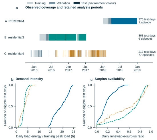
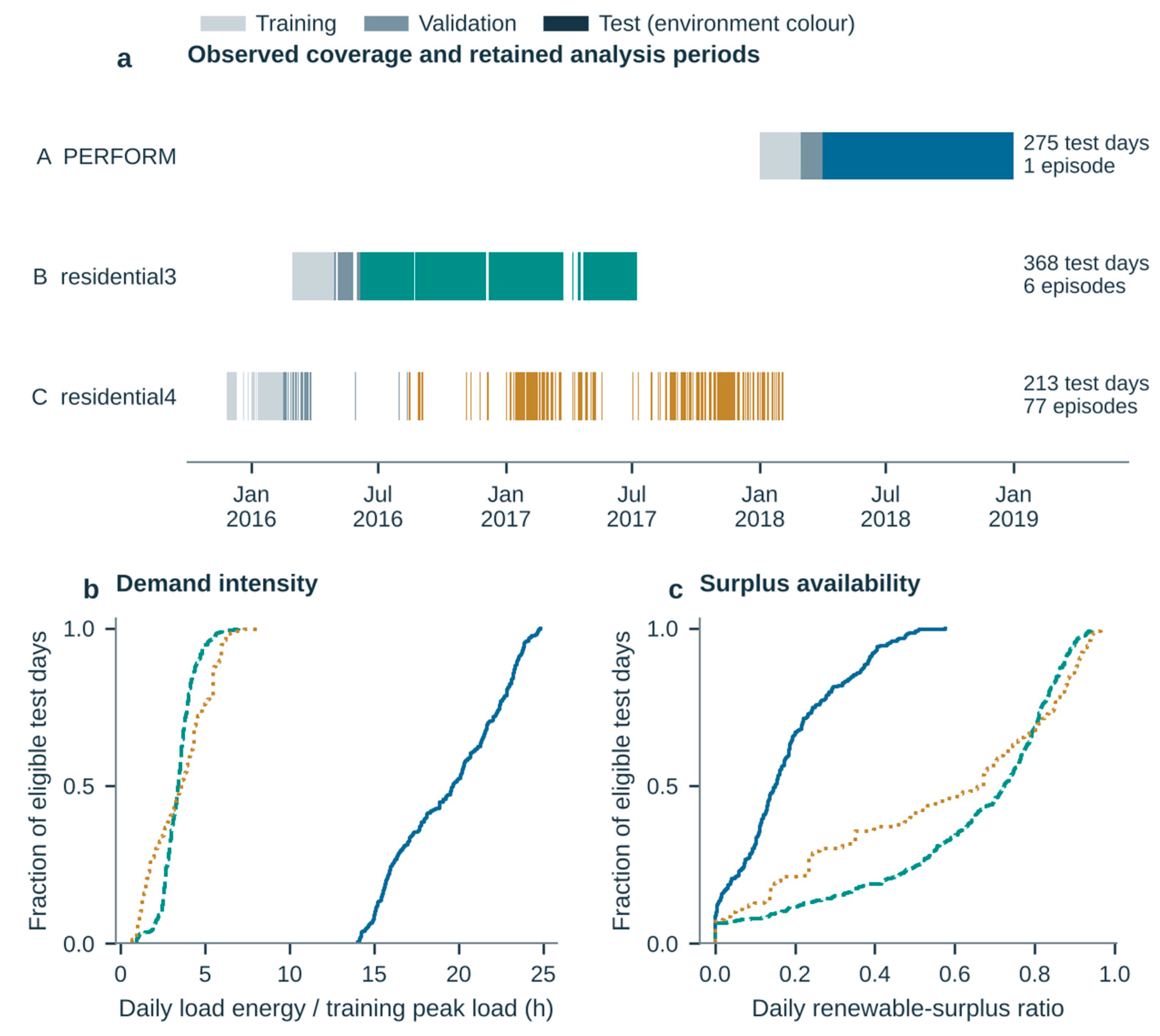
The retained test sets cover 275, 368, and 213 days and serve 20,494.30, 5.198, and 5.054 MWh of load in A, B, and C. Figure 2 separates coverage gaps from operating profile variation. The test period of A is contiguous, whereas B and C contain gaps, and the 213 test days of C form 77 episodes, 43 of them single days. These short episodes limit the evidence on long state histories: fixed-horizon planning prevents the controller from anticipating segment ends, but it cannot reconstruct missing observations or avoid repeated initialization.
Figure 2.
Observation coverage and operating profiles. (a) Training, validation, and test periods of A (PERFORM) and of B and C (OPSD households residential3 and residential4); retained segments preserve gaps, and the labels give test days and episodes (1, 6, and 77 in A, B, and C). (b) Daily load energy divided by the training period peak load, which has units of hours. (c) Daily native-resolution PV surplus share; zero-PV days have undefined surplus share and are omitted from this panel only. Curves in (b,c) are empirical cumulative distributions over eligible test days. In (a), light and medium gray bars mark the training and validation periods, and test periods are shown in the color of each environment (blue, A; teal, B; ochre, C); in (b,c), the same colors and the line styles (solid, A; dashed, B; dotted, C) identify the environments. B and C are separate households within one acquisition project; their distributions do not imply independent system replication.
Validation selects median windows of 30, 60, and 60 days and terminal values of CU 0.14, 0.08, and 0.08/kWh in A, B, and C. For the weighted mean, validation selects a half-life of 14 days and a gain of one in A but a half-life of 30 days and a gain of zero in both households. With zero gain, the weighted-mean forecasts of B and C equal the uncalibrated forecasts, so their 18 configurations duplicate uncalibrated cells; they are retained for completeness and are not replications of active calibration.
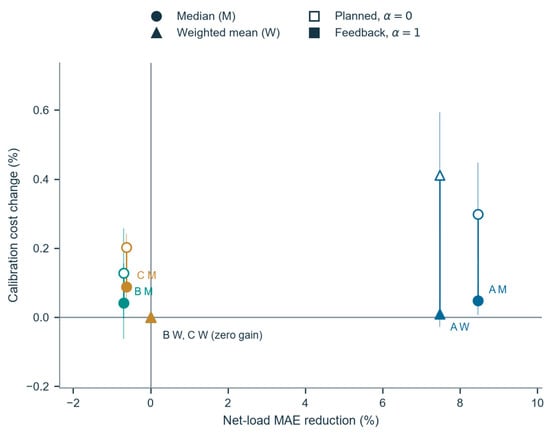
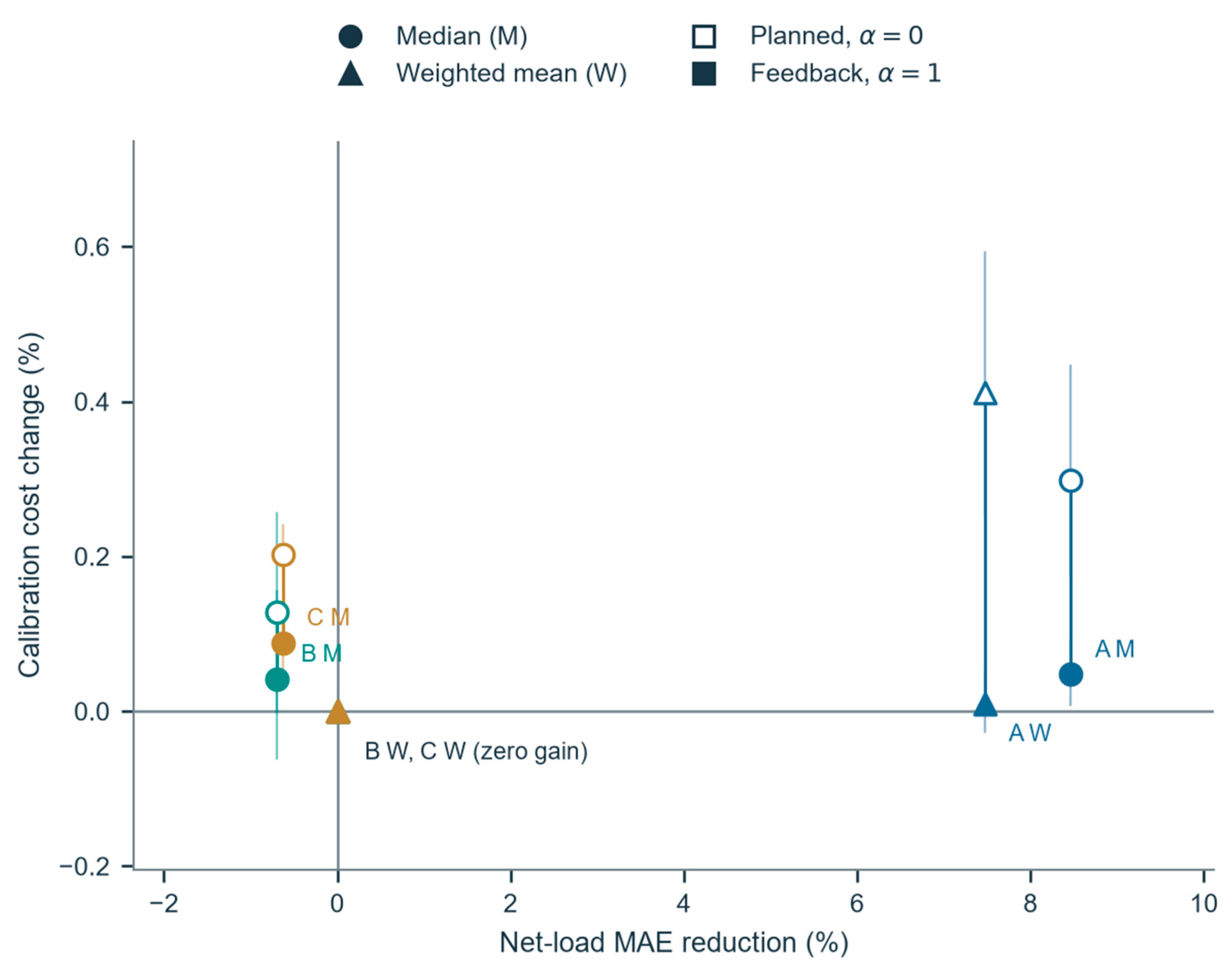
Median calibration reduces A’s first-step net-load mean absolute error (MAE) from 625.277 to 572.333 kW (8.467%), and the weighted mean reduces it to 578.560 kW (7.471%). In B and C, median correction instead increases the MAE, from 0.58054 to 0.58457 kW (0.695%) and from 0.94756 to 0.95352 kW (0.629%), compared with training peak loads of 4.152 and 6.784 kW (Supplementary Table S4); the weighted-mean forecasts remain unchanged (Figure 3). This net-load measure differs from the component MAE criterion used for validation (Section 2.2).
Figure 3.
Accuracy changes and S0 cost effects relative to the uncalibrated forecast at the same execution setting. Marker shape identifies the calibration (circles, median, M; triangles, weighted mean, W), and marker fill identifies the execution (open, planned, α = 0; filled, full feedback, α = 1); the squares in the legend show only the fill convention. Colors identify environments A (blue), B (teal), and C (ochre). Positive horizontal values indicate net-load MAE reduction, so the median-calibrated points of B and C lie at −0.695% and −0.629% (MAE increases), and their weighted-mean points lie at zero because the selected gain is zero. Positive vertical values indicate increased cost. Vertical lines connect the planned (α = 0) and full-feedback (α = 1) cost effects of each treatment. Because the two effects are normalized by different costs (Equation (6)), the length of a line is not the interaction; interactions are given in Section 3.2. Bars are conditional 95% seven-day block intervals from 2000 paired resamples; gaps and segment sizes remain fixed. The test windows had been inspected before the revision protocol was frozen; interval interpretation follows Section 2.5.
Under S0, A’s median correction raises costs by CU +4295.179 (+0.2981%), CU +961.443 (+0.0678%), and CU +672.315 (+0.0476%) at α = 0, 1/2 and 1. Weighted-mean correction raises A’s cost by CU +5924.935 (+0.4112%), CU +1016.020 (+0.0717%), and CU +142.621 (+0.0101%), and the interval of the last value includes zero. In A, improved accuracy is therefore accompanied by a higher point estimate cost at every feedback intensity. In B and C, median correction raises the planned cost by CU 0.40788 (0.128%) and CU 0.64229 (0.202%) and the full-feedback cost by CU 0.12852 (0.042%) and CU 0.27092 (0.089%), so in the households the cost increase accompanies a less accurate forecast. Figure 3 shows both correction methods, including the adverse and zero-gain outcomes.
3.2. Factorial Interaction
Table 3 gives the four endpoint costs in every environment and scenario, and Table 4 gives the resulting calibration effects and interactions in CU, with percentages. Median calibration raises both endpoint costs in every environment and scenario. The S0 interactions are CU −3622.864 (−0.2514%) in A, CU −0.27936 (−0.0876%) in B, and CU −0.37137 (−0.1169%) in C, but their meaning differs between environments. In A, calibration lowers the MAE by 8.467% yet raises costs, and full feedback reduces that increase from CU 4295.179 to 672.315 by about 84%. In B and C, calibration worsens the MAE, and feedback attenuates the cost of an adverse correction. The three negative signs are therefore not three replications of a better forecast costing more. Feedback itself lowers the uncalibrated S0 cost by CU 27,127.090, 11.94806, and 11.84712 (C00 − C01), so the interaction is small relative to the main effect of feedback. The B and C interactions are smaller than one currency unit in magnitude over their retained windows under hypothetical tariffs and do not establish commercially important savings.
Table 3.
Operating costs (CU) of the four endpoint cells in each environment and scenario. Subscripts follow Equation (5) and Figure 1b; costs include the discharged energy proxy and exclude planning preferences and terminal credit.
Table 4.
Median calibration cost effects and interactions in every environment and scenario in CU with percentages in parentheses (Equations (5) and (6)). C10 − C00 and C11 − C01 are the calibration effects under planned execution and full feedback and δ10 and δ11 express them relative to their own uncalibrated cells; I is the interaction, and ι expresses it relative to C00. Positive effects mean that calibration raises costs. Intervals are conditional 95% seven-day block intervals for I; test outcomes had been inspected before the revision protocol was frozen, so they are descriptive. Entries are rounded independently, so differences of rounded entries can deviate from the tabulated interaction in the last digit.
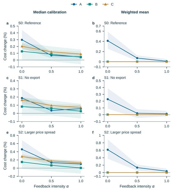
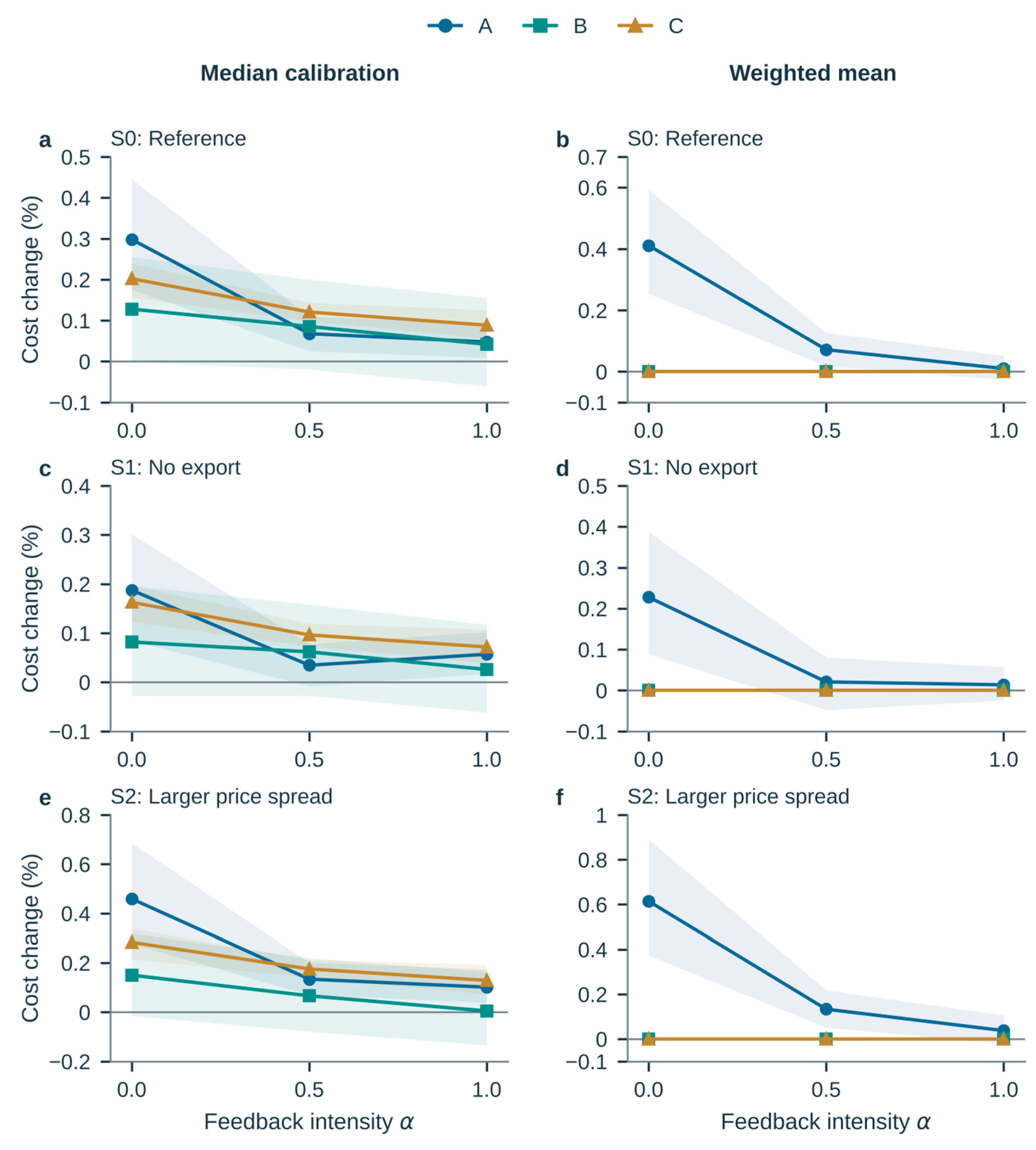
S2’s higher peak price increases the magnitude of the negative interaction in all environments to CU −6504.017, −0.62696, and −0.65468 in A, B, and C, whereas prohibiting export in S1 reduces it to CU −1963.559, −0.22863, and −0.35619 (Table 4). B’s S1 interval, CU [−0.54684, +0.07166] ([−0.137%, +0.018%]), includes zero. Intermediate feedback generally reduces the median calibration cost effect, but three intensities do not establish a smooth substitution law (Figure 4). Zero-gain household treatments give zero contrasts by construction.
Figure 4.
Calibration cost effects across feedback intensity and tariff scenarios. (a) Median calibration, S0; (b) weighted-mean calibration, S0; (c) median calibration, S1; (d) weighted-mean calibration, S1; (e) median calibration, S2; (f) weighted-mean calibration, S2. Each cost effect is relative to the uncalibrated forecast at the same feedback intensity. Shaded bands are conditional 95% intervals from seven-day block resampling of test days that had been inspected before the protocol was frozen; axis limits enclose every point and interval endpoint, including those at α = 0. S1 prohibits export; S2 raises the peak price. The weighted-mean lines of B and C are zero by construction because validation selected zero gain. The interaction uses absolute cost contrasts before normalization, so subtracting plotted percentages does not recover it; Table 4 gives the endpoint values in CU.
3.3. Cross-Dataset Evidence
The households extend the evidence beyond the 2018 benchmark, but not as replications of a successful forecast improvement: median correction worsens their forecast error, and validation selects no weighted-mean correction. What the three environments share is narrower. The specified request rule attenuates the cost effect of calibration whether that calibration improved accuracy, as in A, or degraded it, as in B and C.
The uncertainty estimates reflect different data coverage, and because test outcomes had been inspected before the protocol was frozen, they are descriptive. B’s S0 seven-day interval, CU [−0.55989, −0.02126], lies below zero, whereas its three-day interval, CU [−0.55572, +0.00261] ([−0.1742%, +0.0008%]), includes positive values. In C, only 59 of the 213 days belong to observed segments longer than seven days and can vary across seven-day resamples; the other 154 days enter as fixed segment totals. This is a resampling count, not a count of days with non-zero effects, and the narrow band does not account for missing periods or for the pattern of episode occurrence. Supplementary Table S11 reports every block length; the monthly contributions are available from the first author upon request. We make no pooled site-level significance claim.
3.4. Plan to Execution Mechanism
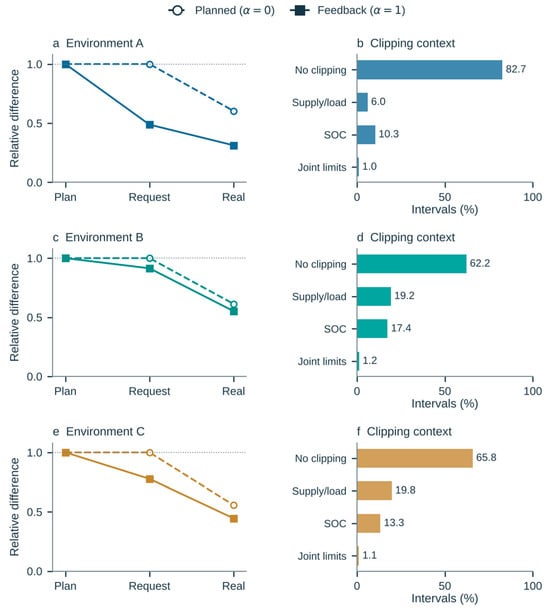
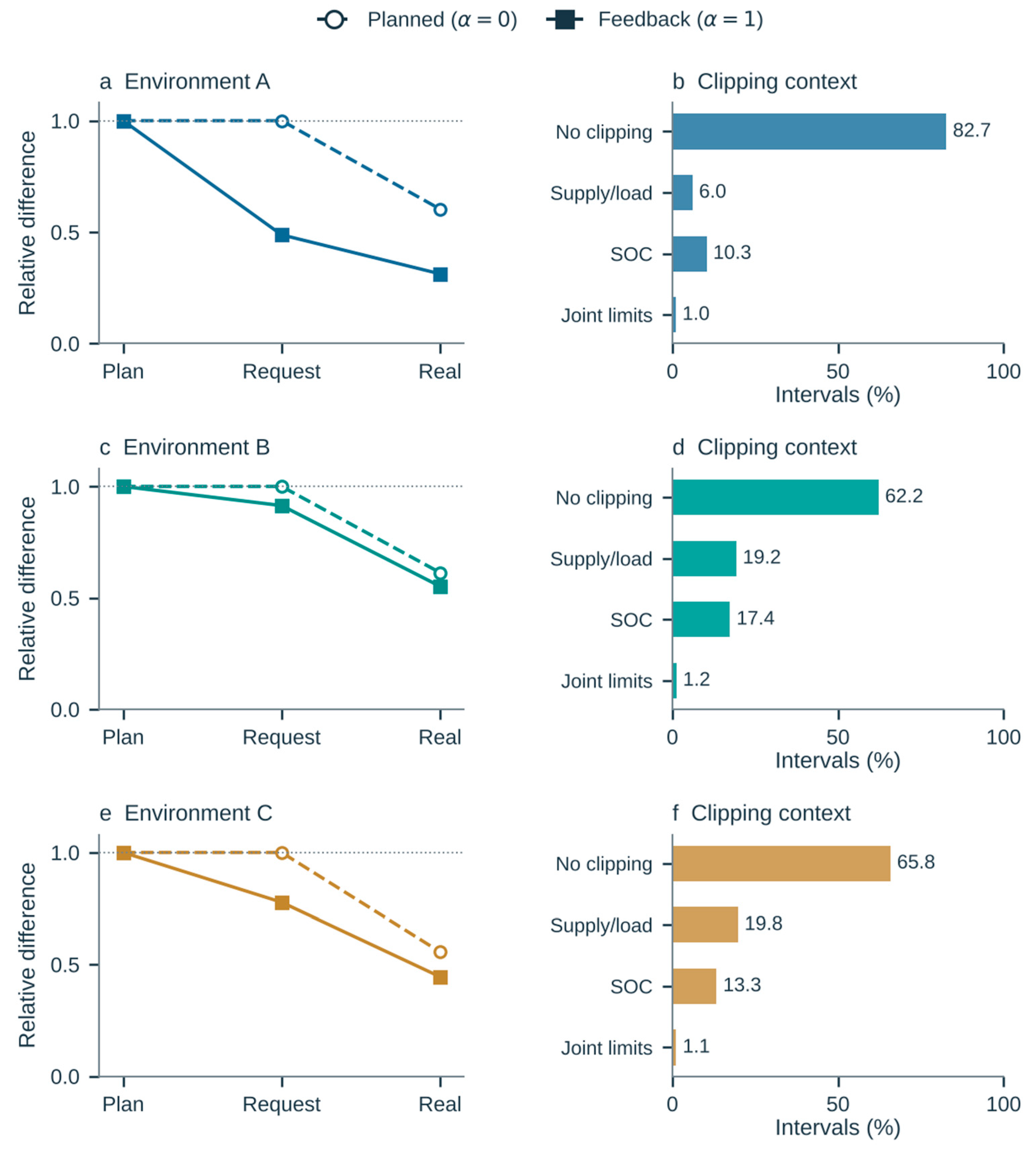
For A with full feedback, the paired absolute energy difference is 199,576.88 kWh in the plans, 97,326.80 kWh in the requests, and 62,384.22 kWh in the realized actions. The request-to-plan ratios are 0.488, 0.914, and 0.777 in A, B, and C: request replacement removes about half of the planned difference in A but less than a quarter in B and C. Under planned execution, requests retain the whole plan difference, and the reduction occurs during physical clipping (Figure 5).
Figure 5.
Action differences through the execution stages and the associated clipping conditions. Left panels (a,c,e) express paired charging and discharging energy differences relative to the plan difference; the realized endpoint is the transmission ratio R of Equation (7). Right panels (b,d,f) give the percentage of native execution intervals in each clipping class: no clipping, supply/load limit, SOC limit, or joint limits (two or more limits binding at once). The bars of each panel therefore sum to 100% of intervals and are not energy or cost shares. Rows correspond to A, B, and C. These counts describe physical conditions and are not independent causal contributions to cost.
Full feedback gives the paired controllers the same request whenever neither plans discharge. Their realized energy differences in these intervals nevertheless total 12,778.02, 13.44, and 8.57 kWh in A, B, and C. Power and surplus limits are shared, so these unequal actions under identical requests arise from the charging headroom left by different SOC histories. Starting both controllers from a common SOC removes the request and realized differences in this shared inactive group, as the rule requires; how often the group occurs, and how much it contributes to costs, depend on the propagated trajectories. The cost contrast is concentrated in other hours. In A, the calibration effect under full feedback, CU +672.315, splits into CU +437.844 in the 191 h with unequal planned discharge gates, CU +265.897 in the 721 h in which both plans discharge and CU −31.425 in the 5688 h in which neither does. The corresponding parts are CU −0.07291, +0.23957, and −0.03815 in B (74, 2412, and 6346 h; total CU +0.12852) and CU +0.11722, +0.11453, and +0.03917 in C (57, 1429, and 3626 h; total CU +0.27092). These parts partition the calibration effect under feedback, not the interaction.
Table 5 compares the propagated trajectories with the common-state shadows. Replanning each hour changes the plans as well as the realized actions and recomputes gate membership. The lower shadow ratios therefore compare a different set of plans: they indicate dependence on the state history but do not assign a causal mediation fraction to the attenuation of the original plan differences.
Table 5.
Full-feedback action differences under S0. Energy columns sum absolute charge and discharge differences (kWh); R1 is Equation (7). Shadows restart and replan hourly from a common SOC and do not define long-run operating bills.
In the C doubled-storage variant (Section 2.6), the S0 interaction becomes CU +0.37041 (+0.1242%), with conditional 95% interval CU [+0.16072, +0.56744] ([+0.0539%, +0.1903%]), and the state-adjusted value remains positive at CU +0.43410. Purchase, export revenue, and proxy components contribute CU +0.44744, −0.04217, and −0.03485. Within this variant, the calibration contrast C1j − C0j shows that calibrated imports fall by 1.340 kWh under planned execution (j = 0) and by 0.289 kWh under full feedback (j = 1), yet purchase expenditure rises by CU 0.1937 and 0.6411 because purchases shift towards peak hours; the corresponding peak price penalty grows from CU 0.48169 to 1.02361. Transmission still falls from 0.521 to 0.409, so smaller action differences do not determine the economic sign.
In A, a flat purchase price gives an interaction of CU +338.080 (+0.0210%), with conditional 95% interval CU [−407.095, +1034.618] ([−0.0253%, +0.0643%]). Purchases, export revenue, and the proxy contribute CU +942.175, −380.890, and −223.206, so opposing components leave a small positive point estimate whose interval includes zero despite substantial action changes; transmission changes from 0.690 to 0.700. The sign of this interaction is therefore unresolved; the result shows neither a zero interaction nor that flat prices eliminate forecast value. Prespecified maximum and minimum daily events are shown in Supplementary Figures S1 and S2, and the training threshold regime results are available from the first author upon request; where the preceding history is missing, this is stated rather than reconstructed.
3.5. Transferability and Sensitivity
Transferring A’s residual window and terminal value settings to B reverses the interaction point estimate from CU −0.27936 (−0.0876%) to CU +0.28135 (+0.0868%), with conditional 95% interval CU [−0.19502, +0.86107] ([−0.0601%, +0.2656%]), which includes zero. Calibration then lowers costs relative to the same transferred uncalibrated forecast at both endpoints, but the transferred policies cost more in absolute terms than the target-selected policies. Because two settings change, including the terminal valuation of the uncalibrated forecast, the result cannot be read as calibration portability. B to C and C to B transfers select identical settings and provide no differentiating test.
Observed future information references (Section 2.6) reduce S0 costs under planned execution by CU 25,287.004 (1.755%), CU 36.26657 (11.370%), and CU 28.93997 (9.110%) in A, B, and C and under full feedback by CU 2555.006 (0.181%), CU 19.65812 (6.403%), and CU 13.80833 (4.515%). Future means replace predictions only where available, with recorded coverage and causal fallback elsewhere. These finite-horizon references are non-deployable information diagnostics, not guaranteed global lower bounds. The value that these references still show at the households, although the selected weighted-mean gain there is zero, separates the potential value of information from the ability of these corrections to capture it.
The selected fixed margins are zero in all environments. Relative to calibrated operation without margins, adaptive margins increase planned execution costs by CU 1007.437, 1.375, and 0.615 and change full-feedback costs by CU −28.849, −0.069, and −0.331 in A, B, and C. These mixed outcomes do not establish adaptive margin superiority.
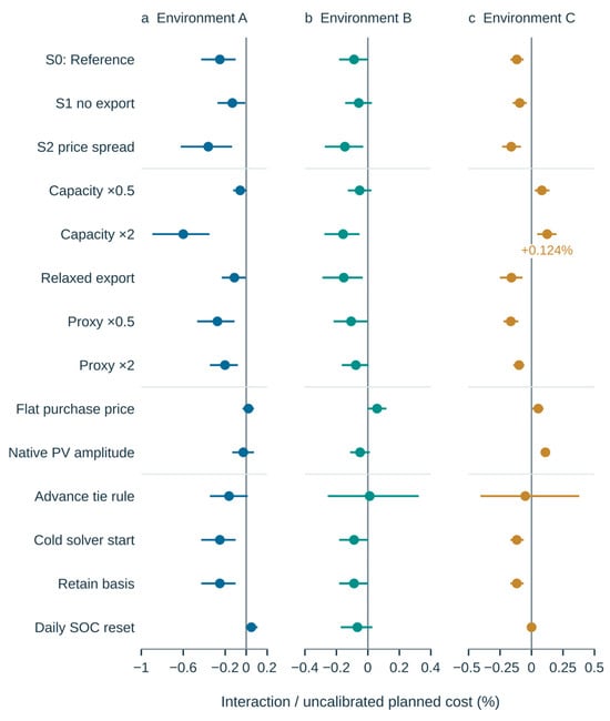
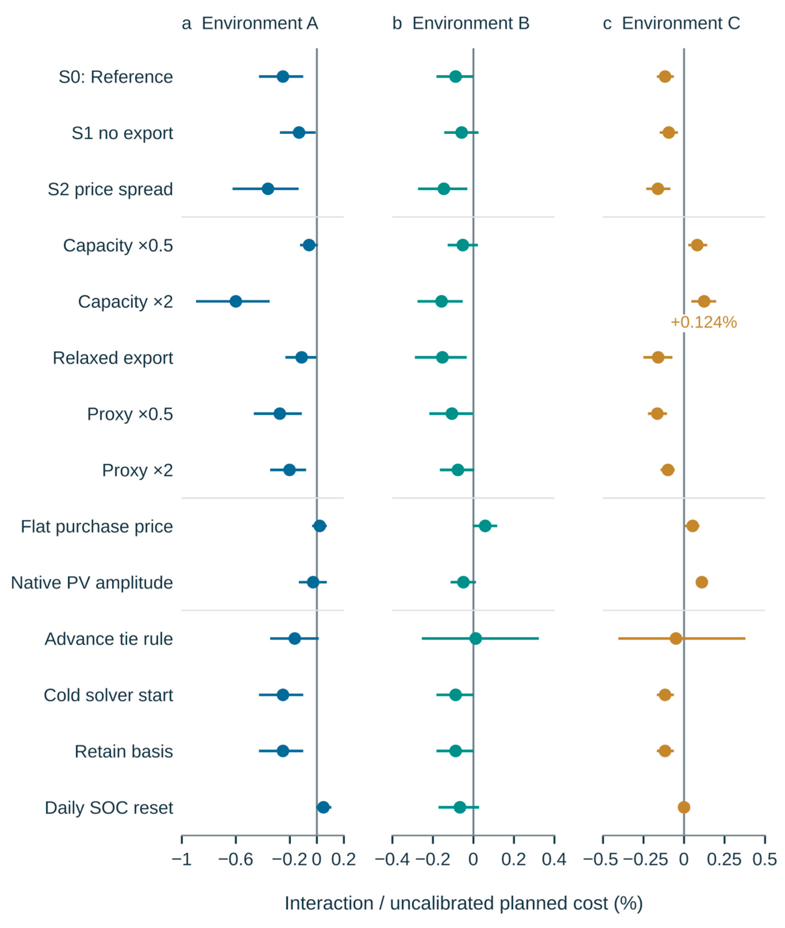
Figure 6 summarizes the primary scenarios and the registered variants. Of the 42 conditional 95% intervals, 26 lie wholly below zero, 6 lie wholly above zero, and 10 include zero. The six positive intervals belong to A with daily SOC resets, CU +719.511 (+0.0499%); B with a flat purchase price, CU +0.19747 (+0.0587%); and C with halved storage, CU +0.27811 (+0.0825%), doubled storage, CU +0.37041 (+0.1242%), a flat purchase price, CU +0.18288 (+0.0527%), and native PV amplitude, CU +0.41964 (+0.1110%). Intervals include zero for A with a flat purchase price, native PV amplitude and the throughput-advancing tie rule; for B under S1 and with halved storage, native PV amplitude, the throughput-advancing tie rule and daily SOC resets; and for C with the throughput-advancing tie rule and daily SOC resets. Three of these ten have positive point estimates: A with a flat purchase price, CU +338.080 (+0.0210%); B with the throughput-advancing tie rule, CU +0.03716 (+0.0121%); and C with daily SOC resets, CU +0.000339 (+0.000111%). Raw and state-adjusted interactions differ in sign for C with a flat purchase price (CU +0.18288 and −0.01519), A with daily SOC resets (CU +719.511 and −1342.236), and C with daily SOC resets (CU +0.000339 and −0.19210). Cold hourly solver starts and retained bases reproduce the primary interactions to the reported precision. These sign changes show that the interactions, and particularly the small household effects, depend on storage size, price structure, action selection, and retained energy accounting.
Figure 6.
Sensitivity of the interaction to physical, economic, and numerical settings (Section 2.6). (a) Environment A; (b) environment B; (c) environment C. Points show raw cost four-cell interactions divided by C00 of the same setting; bars are conditional 95% seven-day block intervals over test days that had been inspected before the protocol was frozen. The first three rows repeat the primary scenarios S0–S2; each variant re-evaluates all four cells under S0 with frozen parameters, and capacity changes scale energy and power together. Points to the right of zero are positive interactions; the labeled doubled-storage value in C is +0.124% (CU +0.37041). Each environment has its own horizontal scale, and the axis limits enclose every interval endpoint; where an interval is narrower than the marker, the marker covers it. Section 3.5 lists the settings whose intervals lie above zero or include zero, with values in CU.
We checked the saved records and, separately, reran the optimization. Across 265 configurations, the records contain 1,804,800 hourly plans, plus the common-state shadows. Recomputing the balance, SOC, and costs from 11,971,200 saved intervals verifies the accounting. The separate four-cell rerun for C solves 20,448 plans and reproduces the core results within the declared tolerances. In twenty-eight additional checks, perturbing future information leaves the current forecasts and actions unchanged.
4. Discussion
A cost increase after an accuracy gain has precedents. Forecast skill and economic value diverge in microgrid operation [9] and in PV–battery market participation [10], whereas under peak pricing, cost rises roughly linearly with PV error [8]. Closed-loop re-optimization from measured state, and the non-additivity of forecast information and feedback effects, have also been reported [17], and rolling and declaration-based PV–storage operation under forecast uncertainty has been evaluated [22,23]. A’s result, in which median calibration lowers the MAE by 8.467% but raises costs, and C’s reversal under doubled storage are consistent with this literature rather than new in kind. The contribution here is the controlled crossing of two residual calibrations with the charging request rule of Equation (4) under common operating conditions, which identifies where the joint cost effect persists and where it changes direction.
When both plans leave discharge inactive, feedback can replace their different charging instructions with the same request. That cancellation ends at the request stage: earlier decisions may have left different energy headroom, and a forecast change can also shift discharge timing or change which branch of the rule applies. The common-state shadows probe this dependence, although their replanning changes the plans being compared. Cost then depends on the timing of the remaining actions. In the capacity reversal, imports and transmission fall while purchases shift towards expensive periods. Under flat prices, opposing transaction components largely cancel and leave a small positive interaction whose interval includes zero.
In the system studied, the economic effect of a forecast change depended on the execution permissions. With complete charging request replacement, a change in planned charging had little immediate effect while the discharge gate was unchanged, whereas changes to discharge timing, subsequent SOC, or peak-period transactions still mattered. Reporting signed purchases and sales by price period made these effects visible when energy totals concealed them. The sign change under doubled storage in C is a single case and does not establish a general rule for forecast evaluation or for the value of storage; it shows only that, in this environment, the sign of the interaction depended on storage size.
Feedback mainly reduces the extra cost introduced by calibration in the primary cases. Whether it can replace an economically useful forecasting service remains open: median correction worsens household forecast error, and validation selects zero correction for the weighted-mean alternative. The observed future information diagnostics still show value at the households under the simulated architecture, which points to information that the tested residual corrections fail to capture. Given the small household cost differences, investment and sizing decisions would need evidence from a stronger predictor evaluated with actual tariffs, operating services, and implementation costs.
B and C are separately metered households from the same acquisition project and geographical area, processed in the same way. Their load is reconstructed, and the effects of source regularization cannot be undone, hence the qualification “measured-source”. Gaps in C interrupt long SOC histories. A fixed planning horizon prevents the controller from anticipating episode ends but still requires repeated initialization after gaps. The conditional block intervals omit uncertainty associated with missing periods and between-site differences. Native interval averages allow for energy feasibility checks without resolving instantaneous hardware behavior.
The declared hierarchical selection gives stable results across the tested solver starts, although the opposite selection changes small interactions. Joint parameter transfer also leaves the effects of residual history and terminal valuation entangled. The feasible set excludes grid charging, battery export, flexible demand, demand charges, and network/inverter constraints. Calendar aging, thermal effects, and state-dependent damage are absent from the constant throughput charge. Earlier outcomes had already been inspected when the revision was designed, so the frozen reruns provide traceable revision validation rather than prospective confirmation. These boundaries confine the findings to operating mechanisms in the investigated environments and do not support universal substitution or deployment claims.
5. Conclusions
In one model-generated benchmark and two measured-source households, crossing forecast calibration with a charging-only feedback rule shows that feedback changes the cost effect of calibration. All nine primary endpoint interactions (three environments × three tariff scenarios) are negative, but they do not describe one phenomenon. In A, median calibration lowers the MAE by 8.467% and raises costs, and feedback removes most of that increase (S0 interaction CU −3622.864, −0.251%). In B and C, median calibration worsens accuracy, the weighted mean is not applied because its selected gain is zero, and feedback attenuates the cost of that adverse correction by CU 0.279 and 0.371 over the test windows (−0.088% and −0.117%).
Stage records trace immediate request replacement and the constraints imposed by accumulated SOC: identical requests can lead to different actions, and replanning from a common state changes the contrast, although this diagnostic does not identify causal mediation. Doubled storage in C reverses the interaction to CU +0.370 (+0.124%), and a flat price in A gives CU +338 (+0.021%) with an interval that includes zero. In these cases, transaction timing and cancellation between cost components, rather than forecast accuracy or action transmission alone, determined the result.
The evaluation traces forecast changes through plans, requests, physical actions, and stored energy to operating cost. The findings apply to the tested restricted feedback architecture and illustrative tariffs; their relevance to deployment requires richer independent measurements and validation against specific operating services.
Supplementary Materials
The following supporting information can be downloaded at https://www.mdpi.com/article/10.3390/en19215067/s1, Supplementary File S1: Supplementary Methods and Results, comprising Sections S1–S7, Tables S1–S11, and Figures S1–S3 (complete model and implementation, closest study comparison, data registry and frozen selections, complete operating contrasts and action records, conditional uncertainty, extreme events, transfer and secondary results, and traceability records).
Author Contributions
Conceptualization, X.-Y.L.; methodology, X.-Y.L.; software, X.-Y.L.; validation, X.-Y.L.; data curation, X.-Y.L. and Y.-X.C.; writing—original draft preparation, X.-Y.L., Y.-X.C., and Y.-S.C.; writing—review and editing, X.-Y.L. and Y.-S.C. All authors have read and agreed to the published version of the manuscript.
Funding
This research received no external funding. The APC was funded jointly by Xuan-You Liu and Yao-Xian Cui.
Institutional Review Board Statement
Not applicable.
Informed Consent Statement
Not applicable.
Data Availability Statement
The original input datasets are openly available from ARPA-E PERFORM (https://doi.org/10.25984/1891136) and from Open Power System Data Household Data, version 2020-04-15 [37,38]. Processed input data, simulation results, and analysis code supporting this study are available from the first author, Xuan-You Liu (liuxuanyou@cu.ac.kr), upon request.
Acknowledgments
During the preparation and revision of this manuscript, the authors used OpenAI Codex (GPT-6.1-Sol; OpenAI) and Claude (Opus 5.5; Anthropic); their uses are described in Section 2.7. The authors take full responsibility for the content of this publication.
Conflicts of Interest
The authors declare no conflicts of interest.
Abbreviations
The following abbreviations are used in this manuscript:
| BESS | battery energy storage system |
| CU | currency unit (generic, hypothetical tariffs) |
| ERCOT | Electric Reliability Council of Texas |
| LP | linear program |
| MAE | mean absolute error |
| MPC | model predictive control |
| OPSD | Open Power System Data |
| PV | photovoltaic |
| S0, S1, S2 | reference, no export, and high peak price tariff scenarios |
| SOC | state of charge |
| UTC | Coordinated Universal Time |
Appendix A. Data Preparation and Sample Splits
Appendix A.1. Eligibility and Episodes
We exclude intervals with missing endpoints, source interpolation, negative meter differences, or negative reconstructed load. Source flags affect 5.86% and 5.43% of the B and C intervals; the final invalid fractions, which overlap with the flagged intervals, are 5.95% and 6.75%. An hour is eligible only if all of its native intervals are retained, and a UTC day is eligible only if all of its hours are eligible. Missing execution observations are left unfilled. After an excluded day, a new episode starts without carrying over the previous state. A, B, and C contain 1, 6, and 77 test episodes, including 43 single-day episodes in C. The data registry documents exclusions, licenses, and the unresolved limits on raw missingness. Coverage and meter interpretability determined the choice of households residential3 and residential4 before costs were evaluated under the redesigned experiment; household residential6 remains in the screening record. The released records include source regularization, and the original wiring, nameplate capacities, and absence of unobserved storage cannot be verified.
Appendix A.2. Chronological Splits
We retain the original chronological splits. For A, training covers 1 January–28 February 2018, followed by validation in March 2018. For B, training covers 29 February–28 April 2016, with eligible validation days through 5 June 2016. For C, eligible training days fall within 27 November 2015–15 February 2016, and validation ends on 12 August 2016. B and C each supply 60 training days and 30 validation days. Earlier test outcomes had already been inspected when the revision protocol was frozen. The present evaluation is therefore a revision validation, and the test sets cannot be described as prospectively unseen.
Appendix A.3. Time Conventions
Tariffs and residual groups follow local clock time. Elapsed time and forecast availability use UTC, so the repeated local hour at the daylight saving transition retains two distinct UTC identities.
References
- Kull, T.; Zeilmann, B.; Fischerauer, G. Field-Ready Implementation of Linear Economic Model Predictive Control for Microgrid Dispatch in Small and Medium Enterprises. Energies 2021, 14, 3921. [Google Scholar] [CrossRef] [Scilit]
- Pereira, L.; Bansal, R.C.; Kumar, A.; Naidoo, R.M. Integrated forecasting and MPC framework for cost-optimised solar-battery energy management. Sol. Energy 2026, 314, 114720. [Google Scholar] [CrossRef] [Scilit]
- Quan, H.; Ge, Y.; Liu, B.; Zhang, W.; Srinivasan, D. A deep-learning algorithm with two-stage training for solar forecast post-processing. Sol. Energy 2024, 273, 112504. [Google Scholar] [CrossRef] [Scilit]
- Marrocu, M.; Massidda, L. Estimating the value of ECMWF EPS for photovoltaic power forecasting. Sol. Energy 2024, 279, 112801. [Google Scholar] [CrossRef] [Scilit]
- Yang, H.; Jiang, B.; Wang, Y.; Wang, Q.; Geng, H. Improved probabilistic forecasting for solar photovoltaic generation via CVAE with continuous-discrete mixture distributions. Sol. Energy 2026, 305, 114209. [Google Scholar] [CrossRef] [Scilit]
- Zhu, J.; He, Y. A novel photovoltaic power probabilistic forecasting model based on monotonic quantile convolutional neural network and multi-objective optimization. Energy Convers. Manag. 2025, 323, 119219. [Google Scholar] [CrossRef] [Scilit]
- Lauret, P.; David, M.; Le Gal La Salle, J.; Lorenz, E.; Perez, R.; Voyant, C. A simple method for quickly estimating solar irradiance forecast errors. Sol. Energy 2025, 301, 113821. [Google Scholar] [CrossRef] [Scilit]
- Schmitt, T.; Rodemann, T.; Adamy, J. The Cost of Photovoltaic Forecasting Errors in Microgrid Control with Peak Pricing. Energies 2021, 14, 2569. [Google Scholar] [CrossRef] [Scilit]
- Manzolini, G.; Fusco, A.; Gioffrè, D.; Matrone, S.; Ramaschi, R.; Saleptsis, M.; Simonetti, R.; Sobic, F.; Wood, M.J.; Ogliari, E.; et al. Impact of PV and EV Forecasting in the Operation of a Microgrid. Forecasting 2024, 6, 591–615. [Google Scholar] [CrossRef] [Scilit]
- Campos, R.A.; Martins, G.L.; Rüther, R. Assessing the influence of solar forecast accuracy on the revenue optimization of photovoltaic + battery power plants in day-ahead energy markets. J. Energy Storage 2022, 48, 104093. [Google Scholar] [CrossRef] [Scilit]
- Fiori Maccioni, A.; Sbaraglia, S.; Mahmoudvand, R.; Zedda, S. A Comparative Analysis of Price Forecasting Methods for Maximizing Battery Storage Profits. Energies 2025, 18, 3309. [Google Scholar] [CrossRef] [Scilit]
- Poti, K.D.; Naidoo, R.M.; Mbungu, N.T.; Bansal, R.C. Optimal hybrid power dispatch through smart solar power forecasting and battery storage integration. J. Energy Storage 2024, 86, 111246. [Google Scholar] [CrossRef] [Scilit]
- Raj, R.P.; Kowli, A. Handling forecast uncertainty and variability in solar generation to mitigate schedule deviation penalties. Sol. Energy 2024, 271, 112401. [Google Scholar] [CrossRef] [Scilit]
- Cheng, L.; Zang, H.; Trivedi, A.; Srinivasan, D.; Wei, Z.; Sun, G. Mitigating the Impact of Photovoltaic Power Ramps on Intraday Economic Dispatch Using Reinforcement Forecasting. IEEE Trans. Sustain. Energy 2024, 15, 3–12. [Google Scholar] [CrossRef] [Scilit]
- Cheng, B.; Yan, L.; Nan, X.; Sun, B. Risk-Aware Rolling-Horizon Scheduling of a PV–Battery–EV Charging Station via Adaptive Conformal Prediction. Energies 2026, 19, 4093. [Google Scholar] [CrossRef] [Scilit]
- Brown, P.; Göl, M. Bayesian probabilistic photovoltaic power forecasting and stochastic model-predictive control for an agricultural microgrid. Sol. Energy 2026, 304, 114197. [Google Scholar] [CrossRef] [Scilit]
- Zhang, Y.; Xia, M.; Xia, X.; Yue, J.; Chen, G. Closed-Loop Economic Dispatch of Battery Energy Storage Systems Considering Battery Degradation. Energies 2026, 19, 4539. [Google Scholar] [CrossRef] [Scilit]
- Li, D.; Ren, L.; Liu, F.; Gao, J.; Ma, K. Two-time scale microgrid scheduling based on power fluctuation mitigation priority and model predictive control. Energy 2025, 324, 135760. [Google Scholar] [CrossRef] [Scilit]
- Saleem, M.I.; Saha, S.; Izhar, U.; Ang, L. Bi-Layer Model Predictive Control strategy for techno-economic operation of grid-connected microgrids. Renew. Energy 2024, 236, 121441. [Google Scholar] [CrossRef] [Scilit]
- Zhao, J.; Liu, Z.; Ji, H.; Yu, L.; Yuanlv, Z.; Duan, S.; Song, G.; Yu, H.; Li, P. Lightweight probability forecasting and local control of photovoltaic integrated with energy storage system in active distribution networks. Renew. Energy 2026, 258, 124979. [Google Scholar] [CrossRef] [Scilit]
- Saha, S.; Elliott, M.; Huda, S.; Abawajy, J.; Jiang, F.; Oo, A.M.T.; Sun, Y.; Mao, T. Model predictive control-based energy management for microgrids in weak utility grid environments. Int. J. Electr. Power Energy Syst. 2026, 181, 112066. [Google Scholar] [CrossRef] [Scilit]
- Ma, C.; Xu, X.; Pang, X.; Li, X.; Zhang, P.; Liu, L. Scenario-based ultra-short-term rolling optimal operation of a photovoltaic-energy storage system under forecast uncertainty. Appl. Energy 2024, 356, 122425. [Google Scholar] [CrossRef] [Scilit]
- Xu, X.; Ma, C.; Gou, H.; Deng, Z.; Tian, Z. Controllable joint forecast of oversized photovoltaic-energy storage systems considering energy storage flexibility. Energy 2025, 319, 135138. [Google Scholar] [CrossRef] [Scilit]
- Gilabert-Torres, C.; Rus-Casas, C.; Jiménez-Castillo, G.; Muñoz-Rodríguez, F.J. Photovoltaic systems with battery storage: A novel and comprehensive scheduling method for high-consumption facilities. J. Energy Storage 2025, 139, 118858. [Google Scholar] [CrossRef] [Scilit]
- Yaniv, A.; Beck, Y. Optimal battery scheduling in solar-plus-storage grid-connected microgrid for profit and cost efficiency: A use case on an Israeli microgrid. J. Energy Storage 2024, 77, 109697. [Google Scholar] [CrossRef] [Scilit]
- Hu, Z.; Gao, Y.; Sun, L.; Mae, M.; Imaizumi, T. Improved robust model predictive control for residential building air conditioning and photovoltaic power generation with battery energy storage system under weather forecast uncertainty. Appl. Energy 2024, 371, 123652. [Google Scholar] [CrossRef] [Scilit]
- Saleem, M.I.; Saha, S.; Izhar, U.; Ang, L. A stochastic MPC-based energy management system for integrating solar PV, battery storage, and EV charging in residential complexes. Energy Build. 2024, 325, 114993. [Google Scholar] [CrossRef] [Scilit]
- Weng, S.; Ma, T.; Kanzumba, K.; Zhao, F.; Zhang, Y.; Li, B.; Xue, P. Battery capacity design and optimal operation control of photovoltaic-battery system considering electrochemical aging. J. Energy Storage 2024, 79, 110103. [Google Scholar] [CrossRef] [Scilit]
- Amini, M.; Sanjareh, M.B.; Nazari, M.H.; Gharehpetian, G.B.; Hosseinian, S.H. A Novel Model for Battery Optimal Sizing in Microgrid Planning Considering Battery Capacity Degradation Process and Thermal Impact. IEEE Trans. Sustain. Energy 2024, 15, 1435–1449. [Google Scholar] [CrossRef] [Scilit]
- Minh, N.Q.; Linh, N.D.; Khiem, N.T. A mixed-integer linear programming model for microgrid optimal scheduling considering BESS degradation and RES uncertainty. J. Energy Storage 2024, 104, 114663. [Google Scholar] [CrossRef] [Scilit]
- Qian, C.; He, N.; Cheng, Z.; Li, R.; Yang, L. Double-layer optimal scheduling method for solar photovoltaic thermal system based on event-triggered MPC considering battery performance degradation. Energy 2024, 304, 132233. [Google Scholar] [CrossRef] [Scilit]
- Liu, H.; Tang, W. Dynamic battery degradation-informed optimal microgrid scheduling: A prediction-aware two-stage stochastic programming approach with spatiotemporal correlation scenario generation. J. Energy Storage 2026, 165, 122231. [Google Scholar] [CrossRef] [Scilit]
- Lee, Y.; Jeong, J. TSMixer- and Transfer Learning-Based Highly Reliable Prediction with Short-Term Time Series Data in Small-Scale Solar Power Generation Systems. Energies 2025, 18, 765. [Google Scholar] [CrossRef] [Scilit]
- Langtry, M.; Wichitwechkarn, V.; Ward, R.; Zhuang, C.; Kreitmair, M.J.; Makasis, N.; Xuereb Conti, Z.; Choudhary, R. Impact of data for forecasting on performance of model predictive control in buildings with smart energy storage. Energy Build. 2024, 320, 114605. [Google Scholar] [CrossRef] [Scilit]
- Karttunen, L.; Jouttijärvi, S.; Jasielec, J.J.; Niskanen, J.; Huerta, H.; Ranta, S.; Miettunen, K. The impact of battery scheduling strategies on profitability considering battery usage costs and dynamic electricity pricing in Nordic residential PV–battery system. J. Energy Storage 2026, 154, 121301. [Google Scholar] [CrossRef] [Scilit]
- Lundmark, L.; Golzar, F.; Guedez, R.; Astaneh, M. A validated forecasting model for optimizing dispatch schedules of PV–battery system in grid-connected apartment buildings. Appl. Energy 2026, 404, 127123. [Google Scholar] [CrossRef] [Scilit]
- National Renewable Energy Laboratory. ARPA-E PERFORM Datasets [Data Set]; Open Energy Data Initiative (OEDI). 2022. Available online: https://data.openei.org/submissions/5772 (accessed on 29 September 2026).
- Open Power System Data. Data Package Household Data, Version 2020-04-15. 2020. Available online: https://data.open-power-system-data.org/household_data/2020-04-15/ (accessed on 29 September 2026).
- Huangfu, Q.; Hall, J.A.J. Parallelizing the dual revised simplex method. Math. Program. Comput. 2018, 10, 119–142. [Google Scholar] [CrossRef] [Scilit]

Disclaimer/Publisher’s Note: The statements, opinions and data contained in all publications are solely those of the individual author(s) and contributor(s) and not of MDPI and/or the editor(s). MDPI and/or the editor(s) disclaim responsibility for any injury to people or property resulting from any ideas, methods, instructions or products referred to in the content. |
© 2026 by the authors. Licensee MDPI, Basel, Switzerland. This article is an open access article distributed under the terms and conditions of the Creative Commons Attribution (CC BY) license.