


Abstract
Speed control of direct-current (DC) drives requires a balance between tracking performance and electrical demand. This study jointly optimizes controller gains, membership geometry, input uncertainty, three z-levels and their weights, and 25 rule consequents in a finite layered fuzzy controller, labeled T3 in the numerical records. A two-stage evaluation separates optimizer performance from controller-architecture comparisons. Stage I compares study-specific HO, CPO, and Hybrid HO-CPO procedures for the same controller, with 5050 objective evaluations per run. Across 20 matched runs, the hybrid achieves the lowest mean cost (107.5093), followed by CPO (114.8554) and HO (131.1904); rank-based tests identify significant differences. Stage II independently tunes T1, IT2, and finite T3 controllers using the same hybrid and evaluation budget. Their mean costs are 106.2192, 104.6669, and 104.6439, respectively, with no significant architecture difference (Friedman p = 0.7047). Tests with parameter variation, measurement noise, alternative operating conditions, reduced inductance, and perturbed objective weights show that the preferred controller depends on the metric and scenario. The layered controller is competitive in simulation, although its small mean-cost advantage over IT2 is accompanied by a longer optimization time.
1. Introduction
Armature-controlled direct-current (DC) motors are used in positioning systems, conveyors, laboratory drives, and low- to medium-power automation. Their electrical and mechanical dynamics can be described through the relationships among armature voltage, current, electromagnetic torque, and shaft speed. Speed regulation becomes more demanding when reference changes coincide with load disturbances and actuator limits. A controller must recover promptly while keeping current and voltage demand acceptable across operating points. Proportional–integral–derivative control remains a standard benchmark, and population-based optimization provides a practical way to tune nonlinear controllers [1,2,3]. Recent studies in Energies have examined fuzzy and nonlinear control for transient regulation and disturbance rejection in AC and permanent-magnet drives [4,5].
Fuzzy control offers a rule-based approach when plant uncertainty or changes in operating conditions limit the usefulness of one fixed linear tuning. Its foundations include Type-1 sets, Mamdani inference, adaptive and model-based schemes, and Type-2 formulations [6,7,8,9,10,11,12,13,14]. In motor drives, speed error and error rate can be mapped directly to a control action, while membership parameters describe the location and uncertainty of linguistic boundaries.
Studies on DC motor drives have examined fuzzy PI/PID, adaptive fuzzy, neuro-fuzzy, and particle-swarm-tuned controllers, including simulation and hardware-oriented implementations with field-current coordination and FPGA realization [15,16,17,18,19,20,21,22]. Many of these designs, however, tune gains or a limited subset of membership parameters while leaving the rule table and uncertainty structure fixed.
Type-3 fuzzy systems introduce an additional membership level beyond Type-2 systems, with reported applications in robotic manipulators, induction-motor drives, and nonlinear dynamic systems [23,24,25,26,27,28,29]. A separate line of work uses finite zSlices to represent general Type-2 sets. These concepts require different mathematical definitions; increasing the number of interval layers alone does not establish a Type-3 system.
This work formulates DC speed regulation as a joint controller-tuning problem. Scaling gains, integral action, membership geometry, input uncertainty, three z-levels and their weights, and the 25 rule consequents form a 61-variable decision vector. The finite layered controller is labeled T3 in the experimental records. Study-specific HO- and CPO-inspired procedures and their hybrid search this common representation. The evaluation first compares the optimizers for a fixed architecture, then compares independently tuned T1, IT2, and layered controllers under a common optimizer and evaluation budget.
1.1. Related Work on Fuzzy Motor-Drive Control
Type-2 control research includes stability analysis, systematic design, and evolutionary tuning [30,31,32,33,34,35,36]. Recent motor-drive applications include hybrid metaheuristic tuning, fuzzy PMSM and BLDC control, PSO-assisted adaptation, and interval Type-2 control on embedded hardware [37,38,39,40,41].
Recent electric-drive research has also developed along complementary directions that are relevant to the present optimization study. Jin et al. proposed a zero-speed sensorless PMSM scheme that combines virtual-flux signal injection with a hybrid active-flux observer, addressing observability and stable operation in the low-speed region [42]. Cheng et al. combined radial-basis-function modeling and ADALINE adaptation for harmonic estimation and suppression in PMSM drives, showing how a hybrid intelligent estimator can be embedded in the drive-control loop [43]. Chen et al. examined dq-axis current distribution and control of a negative-salient PMSM for vehicle applications, paying particular attention to machine-specific operating characteristics and transient behavior [44]. Wang et al. coupled parameter-sensitivity analysis with multiobjective optimization in an electromechanical design problem, illustrating how sensitivity information can be used to interpret and guide optimized solutions [45]. Although these studies concern different machines and control objectives, they provide useful contemporary context for observer design, intelligent compensation, transient control, and sensitivity-aware optimization.
Higher-order fuzzy applications use different membership hierarchies and inference operators [23,24,25,26,27,28,29]. Their performance must therefore be interpreted in relation to the implemented controller and validation conditions. Section 2.1.3 defines the finite layered construction evaluated here.
Many motor-drive studies use Type-1 fuzzy, fuzzy-PID, or interval Type-2 controllers. Fuzzy and PSO-assisted designs have improved speed regulation relative to the conventional or manually tuned controllers used in their respective tests [15,16,17,18,19,20]. Related studies cover DC and BLDC motors, induction motors, and motor-pump systems [41,46,47,48,49,50]. Optimization often targets gains, scaling factors, or selected membership parameters. Joint optimization of the complete rule base, antecedent uncertainty, layer parameters, and output centers has received less attention in this application.
Evolutionary and hybrid metaheuristic approaches have been used to tune fuzzy-controller parameters and structures [24,25,33], including motor-drive applications [37,40,46]. The original Crested Porcupine Optimizer (CPO) and Hippopotamus Optimization (HO) are population-based search methods [51,52]. The present study uses simplified update schemes inspired by these methods. Its optimizer comparisons, therefore, concern the implementations defined in Section 2.3, rather than an independent benchmark of the canonical algorithms.
Table 1 compares the scope of selected theoretical and applied studies. Section 4.4 provide numerical context while retaining the differences in plant models and test conditions.
Table 1.
Selected studies relevant to the scope of the present work.
Research Gap
The study addresses joint parameter optimization and controlled evaluation. Earlier motor-control work commonly tunes gains or selected membership parameters [15,16,17,18,19,20,21,22,27,28,29,37,38,39,40,41,46,47,48,49,50]. Here, the decision vector includes the gains, all membership centers, input uncertainty coefficients, layer parameters, and 25 rule consequents. Stage I compares search procedures for the same layered controller. Stage II compares independently optimized architectures using one optimizer and one evaluation budget.
Within the broader literature, the present contribution is positioned as an optimization-centered controller co-design study for an armature-controlled DC motor. It does not seek to replace PMSM-specific sensorless observers, harmonic-compensation schemes, or dq-axis current-control strategies. Instead, it examines whether controller gains, membership geometry, uncertainty parameters, layer variables, and the rule base can be tuned jointly while keeping optimizer comparison and controller-architecture comparison under explicitly controlled evaluation budgets.
1.2. Main Contributions
The main contribution is a mixed continuous-discrete formulation for jointly tuning 61 controller variables, evaluated through separate optimizer and architecture comparisons. An initial experiment evaluates the intensified hybrid under unequal evaluation effort. Stage I assigns 5050 evaluations to each search procedure for the same layered controller. Stage II applies the same hybrid, plant, objective, and budget to T1, IT2, and finite T3 controllers. Further tests examine parameter variation, noise, an alternative reference/load profile, current protection, inductance, and objective weights.
2. Materials and Methods
The closed-loop system consists of an armature-controlled DC motor, a finite layered fuzzy speed controller, integral action, and voltage-command conditioning. The motor model retains the armature resistance and inductance, torque and back-EMF constants, rotor inertia, viscous friction, and applied load torque. A 1 ms sampling interval is used over 3.2 s. The reference and load schedules test acceleration, deceleration, and disturbance recovery, while the objective monitors both tracking and electrical demand.
Speed error and filtered error rate are the controller inputs. Each normalized input is described by five triangular sets: negative big (NB), negative small (NS), zero (Z), positive small (PS), and positive big (PB). Five optimized consequent centers define the output levels. The Type-1 fuzzy logic controller (T1 FLC) uses deterministic membership grades; the IT2 scheme adds upper and lower antecedent memberships; and the finite T3 scheme evaluates three interval layers at optimized z-levels. All three use a complete 5 × 5 rule base [7,8,9,10,11,12,13,14,30,31,32,33,34,35,36,53].
The controller is tested with a multistep reference and scheduled load-torque changes. A first-order filter smooths the error derivative, and a bounded integral state limits error accumulation. The fuzzy correction is attenuated near the reference. Feedforward, fuzzy, and integral terms are added to form the voltage command, which is subject to a rate limit and amplitude bounds.
The derivative-filter coefficient is 0.92, the integral-state bound is ±150, and the integral contribution uses tanh(0.035 I), where I is the accumulated error. Input normalization uses tanh(Ge e) and tanh(Gde def), with def denoting the filtered error rate. The fuzzy correction is multiplied by 0.40 + 0.60 min(1, |e|/18). The feedforward voltage is R(B ωref + TL)/Kt + Kb ωref. Table 2 lists the nominal voltage and voltage-increment limits.
Table 2.
Simulation settings and driving constraints.
The initial experiment uses HO, CPO, and an intensified HO-CPO hybrid with a population of 50 and 100 outer iterations. The hybrid combines preliminary elite information, additional trial generation, local refinement, an archive, and restarts. That configuration does not equalize the number of objective evaluations. Stage I and Stage II use separate protocols with 5050 evaluations per procedure, including initialization. The results from the two protocols are reported separately.
Candidate controllers are evaluated using tracking error, residual error, overshoot, voltage variation, current-threshold violations, and residual oscillation. The objective for Stage I and Stage II also includes a plateau-tracking term, defined in Section 2.5.1. A quadratic penalty discourages a current above 35 A; the nominal experiments do not impose hard-current saturation. Tracking is additionally summarized by root-mean-square error (RMSE). Cost distributions from 20 runs are compared with Friedman and Iman–Davenport tests, followed by Holm-adjusted Wilcoxon tests when the omnibus result is significant. MATLAB-2023b performs the simulation, optimization, statistical analysis, and output generation.
Figure 1 shows the workflow from decision-vector encoding to closed-loop simulation and statistical evaluation. Controller performance is assessed together with current demand and the voltage constraints.
Figure 1.
Overall workflow for fuzzy-controller co-design and DC motor performance assessment.
2.1. Fuzzy Controller Architectures
2.1.1. Type-1 Fuzzy Logic Controller
A Type-1 fuzzy set A on a universe X assigns a single membership grade μA(x) ∈ [0, 1] to each input x [10,12,14]. The present controller uses five triangular sets for speed error and error rate, together with five output-center values. The optimizer adjusts their centers and overlap. This representation keeps the input partitions and selected consequent levels directly interpretable.
For rule Rij, IF e is Ai AND Δe is Bj THEN u is Cr, the firing strength is the minimum of the two antecedent grades. The output is the firing-strength-weighted average of the selected consequent centers. It is a center-weighted inference scheme rather than the centroid of an aggregated Mamdani output area [12,13]. Gains Ge, Gde, and Gu scale the input and output channels, and integral action is added outside the fuzzy map. The denominator is bounded below by 10−9; when every rule has zero activation, the fuzzy output is zero.
The Type-1 rule base and membership centers are optimized independently under the common plant, objective, population, and evaluation budget. The comparison therefore concerns complete optimized architectures, including their different active search dimensions.
2.1.2. Interval Type-2 Fuzzy Logic Controller
Interval Type-2 fuzzy logic extends the Type-1 description by allowing the primary membership grade itself to occupy an interval. An interval Type-2 set is therefore represented by an upper membership function (UMF) and a lower membership function (LMF); the region between them is the footprint of uncertainty (FOU). This representation is widely used when the location or width of a linguistic boundary cannot be regarded as exact. The basic operations, upper/lower membership representation, and control interpretation of interval Type-2 systems are established in the Type-2 fuzzy literature [7,8,9,11,30,32,33,34,35,36,54,55].
In the IT2 baseline, the optimized centers define the upper triangular membership functions. Each input set has an uncertainty coefficient that contracts its lower triangle about the same apex. Lower and upper rule strengths are calculated with the minimum t-norm and combined as ηwU + (1 − η)wL. Their weighted consequent-center average gives the output, with a denominator floor of 10−9. This implementation uses a blending approximation and does not perform iterative type reduction.
Uncertainty is confined to the antecedents. The error and error-rate sets have optimized upper and lower memberships, whereas each rule selects a crisp consequent from five optimized output centers. No output-side uncertainty coefficient is included in the decision vector. The coincident output curves visualize the center locations and have a zero-width footprint of uncertainty; inference uses the centers rather than the area of an aggregated output set [9,11,30,31,34,35,36,54,55,56,57,58].
2.1.3. Finite z-Slice Layered Controller
Formal Type-3 systems require an additional membership hierarchy [23,26,53,59,60,61]. The α-plane and zSlices studies cited here describe Type-2 representations [54,55,56,57,58]. The present implementation instead constructs three interval layers at optimized z-levels and averages their outputs. The label T3 identifies this finite layered architecture in the numerical records; it does not imply equivalence to a general Type-3 inference or type-reduction operator.
Equation (1) denotes the finite set of layers, where Azl is the interval description at level zl. The positive aggregation coefficients βl in Equation (5) are optimized separately and normalized to sum to one. The finite layer representation follows the z-slice concept used for general Type-2 systems [57,58].
Figure 2 illustrates the layered construction. The horizontal axis is the primary universe, the z-axis identifies the discrete layers, and the vertical axis is membership grade. Each layer contains upper and lower triangular membership functions. The connecting surfaces are visual interpolation; inference only uses the three optimized z-levels.
Figure 2.
Finite interval-layer construction used in the controller labeled T3. Connecting surfaces visualize the relationships among the discrete z-slices.
Equation (2) defines the upper triangular membership function, with support limits a and c and apex b. For an interior set, the support limits are the adjacent optimized centers; the outer limits of the first and last sets are −1 and 1. The membership grade is zero at the support endpoints.
Equation (3) defines the lower triangle. For input-set uncertainty δi and layer zl, the code uses ρil = max(0.20, 1 − δi(1 − zl)), ailL = bi − ρil(bi − ai), and cilL = bi + ρil(ci − bi). The lower support is therefore nested within the upper support. The IT2 baseline uses the same construction at z = 0.
Equation (4) first calculates lower and upper rule strengths using the minimum t-norm, then blends them with η. The same blending convention is used by the IT2 and finite T3 implementations.
In Equation (5), each layer is normalized separately to obtain yl, and the final output is the weighted average of these layer outputs. The consequent cr(i,j) is selected from the shared output-center vector, βl is the normalized positive layer weight, and ε = 10−9. The result is clipped to [−1, 1]. A layer with no active rules contributes zero.
Equations (1)–(5) define the finite layered calculation used in Stage I and Stage II. Its tunable quantities are the membership centers, input uncertainty coefficients, z-levels, layer weights, and rule consequents. The T3 label identifies this implementation throughout the reported results.
2.1.4. Computational Hierarchy and Limiting Cases
Each optimized z-level defines an interval footprint. Across layers, both the interval geometry and the aggregation contribution may change. If all layers coincide, the architecture reduces to a single interval-layer form; if every upper and lower membership pair also coincides, it becomes Type-1-like [9,11,57,58].
These are limiting relations within the numerical architecture. The independently optimized T1, IT2, and finite T3 experiments in Section 3.3 compare complete designs under a common optimizer and evaluation budget. Differences include their active parameter dimensions and tuned rule maps, so the experiment does not isolate uncertainty order as a single causal factor.
2.2. Armature-Controlled DC Motor Model
The armature-controlled DC motor is represented by the coupled electrical and mechanical equations of motion [62,63,64,65,66]. Armature current ia and angular speed ω are the state variables, armature voltage va is the control input, and load torque TL is treated as an external disturbance. Equation (6) balances the applied voltage against the resistive, inductive, and back-EMF terms and Equation (7) balances electromagnetic torque against viscous friction, inertia, and load torque.
Here, R and L are armature resistance and inductance, Kb is the back-EMF constant, Kt is the torque constant, J is rotor inertia, and B is the viscous friction coefficient [62,63,64,65,66,67,68,69,70,71].
Equations (8) and (9) give the electrical and mechanical derivatives used in the simulation [65,66,67,68,69,70,71].
Forward Euler integration advances both states with the sampling period Ts. The current update uses the voltage command at step k and the current and speed from step k−1. The mechanical update uses the previous current; negative computed speed is clipped to zero. Equations (10) and (11) give the recursions [65,66,67,68,69,70].
The model provides current and speed trajectories for evaluating the controller. It excludes converter switching, magnetic saturation, commutation, and other hardware effects [62,63,64,65,66,67,68,69,70,71]. The results therefore describe the stated simulation model.
2.3. Optimization and Evaluation Protocol
The three search procedures use the same bounded 61-variable representation and scalar objective. HO and CPO denote the study-specific updates below, inspired by the original methods [51,52]. Related hybrid and memetic methods provide context for combining search operators [72,73,74,75,76,77,78,79]. The comparisons assess the implementations defined below.
2.3.1. HO-Inspired Search Procedure
The HO-inspired procedure combines attraction to the current best solution, the mean of the five best candidates, and a decaying uniform perturbation, as shown in Equation (12) [52].
In the equal-budget procedure, progress is q = FE/MaxFEs, with FE denoting the evaluations used so far. The coefficients in Equation (12) are αt = 0.85(1 − q), β = 0.35, and γt = 0.04(1 − q). The vectors r1 and r2 are uniform on [0, 1], and u is uniform on [−1, 1].
Each trial is projected onto the variable bounds, structurally repaired, evaluated, and only retained if it improves the incumbent.
Algorithm 1 summarizes this update and selection cycle.
| Algorithm 1. HO-inspired search | |
| Step | Procedure |
| 1 | Initialization: initialize a population X of N candidates randomly within [LB, UB]. |
| 2 | Evaluation: evaluate the fitness f(X) of all candidates. |
| 3 | Selection: identify the current best solution xbest. |
| 4 | While the stopping criterion is not satisfied |
| 5 | Ranking: rank the population according to fitness. |
| 6 | Elite mean: calculate the mean vector of the elite solutions. |
| 7 | For each candidate xi |
| 8 | Generate a trial solution using Equation (12). |
| 9 | Boundary control: apply [LB, UB] and repair infeasible variables. |
| 10 | Evaluation: evaluate the trial fitness. |
| 11 | If the trial fitness is better than f(xi) |
| 12 | Replace xi with the trial solution. |
| 13 | End if |
| 14 | End for |
| 15 | Update the global best solution xbest. |
| 16 | End while |
2.3.2. CPO-Inspired Search Procedure
The CPO-inspired procedure assigns candidates to an exploratory or contracted update according to their current rank [51]. Equations (13) and (14) give the two updates.
The exploratory update uses λ1 = 0.70 and λ2 = 0.45. At progress q, the active group contains max(4, round(max(0.35, 1 − q)Npop)) candidates from the top of the ranked population. Both update modes add Gaussian noise scaled elementwise by (0.025 + 0.02(1 − q))(ub − lb).
The contracted update uses η1 = 0.50, η2 = 0.35, and η3 = 0.15; xr is an auxiliary peer. Every proposal is repaired and evaluated before greedy acceptance.
The two modes retain the same decision vector definition and feasibility repair.
Algorithm 2 summarizes the implemented CPO cycle: mode assignment, trial generation, repair, objective evaluation, greedy replacement, and best-solution update.
| Algorithm 2. CPO-inspired search | |
| Step | Procedure |
| 1 | Initialization: initialize the population X within [LB, UB]. |
| 2 | Evaluation: evaluate f(X) for all candidates. |
| 3 | Selection: identify the initial best solution xbest. |
| 4 | While the stopping criterion is not satisfied |
| 5 | Ranking: rank the population according to fitness. |
| 6 | Ratio calculation: compute the active search ratio. |
| 7 | For each candidate xi |
| 8 | If xi belongs to the active group |
| 9 | Generate a trial solution using Equation (13). |
| 10 | Else |
| 11 | Generate a trial solution using Equation (14). |
| 12 | End if |
| 13 | Boundary handling: apply [LB, UB] and repair infeasible variables. |
| 14 | Evaluation: evaluate the generated trial solution. |
| 15 | If the trial fitness is better than f(xi) |
| 16 | Replace xi with the trial solution. |
| 17 | End if |
| 18 | End for |
| 19 | Update xbest and record the convergence history. |
| 20 | End while |
| 21 | Return xbest and the convergence history. |
2.3.3. Intensified HO-CPO Hybrid
The intensified hybrid in the initial experiment generates several trial moves for each candidate. Its HO-oriented displacement is defined in Equation (15).
ΔH = r1⊙(xbest − xi) + r2⊙(xmean − xi)
The corresponding CPO-oriented displacement is given in Equation (16).
ΔC = r3⊙(xp − xq) + r4⊙(xbest − xi)
An elite-centered local move is added through Equation (17).
ΔL = r5⊙(xelite − xi) + r6⊙(xbest − x2nd)
The weighted fused move is given in Equation (18).
Equations (15)–(18) summarize the combination of HO-oriented, CPO-oriented, local, and fused moves in the intensified hybrid. Their weights vary with progress and recent improvement [72,74,78]. The equal-budget hybrid uses the separate operator-selection procedure described in Section 2.5.1.
The intensified hybrid maintains an archive, preserves elite solutions, performs local refinement, and restarts weak candidates after stagnation. Its initial population includes elites from completed standalone HO and CPO searches. It can also evaluate several trials for one population member. Its effective evaluation effort is therefore greater than that of the standalone procedures, and the experiment measures the performance of the complete configured search [72,74,78].
Algorithm 3 summarizes the intensified procedure. The equal-budget hybrid described in Section 2.5 starts from a shared initial population, without incorporating solutions from completed standalone searches.
| Algorithm 3. Initial intensified HO-CPO hybrid | |
| Step | Procedure |
| 1 | Hybrid initialization: form the population from elite HO and CPO candidates, mixed candidates, and repaired random solutions. |
| 2 | Evaluation and archiving: evaluate the initial population and create an archive of high-quality solutions. |
| 3 | Selection: determine the initial global best solution xbest. |
| 4 | while the stopping criterion is not satisfied |
| 5 | Adaptive weighting: compute weights for HO-based moves, CPO-based moves, and local exploitation. |
| 6 | For each candidate xi |
| 7 | Multi-strategy trial generation: generate an HO-oriented trial using Equation (15). |
| 8 | Generate a CPO-oriented trial using Equation (16). |
| 9 | Generate a local elite trial using Equation (17). |
| 10 | Generate a fused trial using Equation (18). |
| 11 | Trial selection: retain the best-performing candidate among the generated trials. |
| 12 | Variable repair: apply bounds and repair continuous and discrete variables. |
| 13 | Evaluation: evaluate the repaired trial solution. |
| 14 | If the trial fitness is better than f(xi) |
| 15 | Replace xi with the selected trial solution. |
| 16 | End if |
| 17 | End for |
| 18 | Refinement: apply elite jittering and local search around selected high-quality candidates. |
| 19 | Global update: update the archive and xbest. |
| 20 | If stagnation is detected |
| 21 | Restart the weakest portion of the population to maintain diversity. |
| 22 | End if |
| 23 | End while |
2.4. Statistical Comparison
Rank-based tests compare the procedures over 20 trial blocks [80,81]. In Stage I and Stage II, each block shares an initial unit-hypercube population, while update streams use separate recorded seeds. The blocks represent repeated stochastic runs on one control problem, rather than independent plants or datasets [82,83]. Statistical inference is therefore restricted to this optimization setup.
After ranking the procedures within each block, the mean rank assigned to algorithm j is used to calculate the Friedman statistic in Equation (19).
Here, N = 20 is the number of blocks, k = 3 is the number of procedures, and is the mean within-block rank of procedure j. Rejection of the Friedman null indicates an overall rank difference without identifying a particular pair [80].
Because the chi-square approximation can be conservative with small or moderate samples, the Friedman statistic is supplemented by the Iman–Davenport transformation in Equation (20).
Under the null, Equation (20) is compared with an F distribution with k − 1 and (k − 1)(N − 1) degrees of freedom [81].
If the omnibus test is significant, paired procedures are compared with the Wilcoxon signed-rank test. For block i, the paired difference is defined in Equation (21).
di = xi − yi
Zero paired differences are omitted and the remaining absolute differences are ranked. T+ and T− denote the positive and negative rank sums used in Equation (22) [84,85]. Stage I p-values are calculated using the two-sided normal approximation without continuity correction.
W = min(T+,T−)
The signed-rank statistic uses both the direction and ranked magnitude of the paired differences. Its interpretation assumes an appropriate symmetric distribution of paired differences [84,86].
For the three pairwise contrasts, Holm’s sequential adjustment controls the familywise Type I error rate at 0.05 [87]. The smallest ordered p-value is first multiplied by three, the second by two, and the third by one; cumulative maxima enforce monotonic adjusted p-values, capped at one.
Omnibus testing precedes the Holm-adjusted pairwise comparisons [82,87,88]. The tests assess run-level differences within the stated experiment. They neither correct unequal evaluation effort nor establish superiority over other control problems.
2.5. Equal-Budget Evaluation Protocol
2.5.1. Evaluation Stages and Implementation Settings
The equal-budget protocol separates optimizer performance from controller-architecture comparisons. Stage I compares the three optimizers for a fixed layered architecture, with 5050 objective evaluations each. Stage II applies the selected hybrid to independently tuned T1, IT2, and finite T3 controllers under the same budget.
Stage I uses a population of 50. Within each matched block, one unit-hypercube population is mapped to the common 61-variable space. The vector contains Ge, Gde, Gu, Ki, η, three z-levels, three layer weights, five centers and five uncertainty coefficients for each input, five consequent centers, and 25 integer rule entries. The proposal bounds are Ge ∈ [0.002, 0.050], Gde ∈ [0.0001, 0.008], Gu ∈ [1, 80], Ki ∈ [0, 25], η ∈ [0.10, 0.90], z1 ∈ [0.10, 0.40], z2 ∈ [0.35, 0.75], z3 ∈ [0.70, 1.00], and layer weights in [0.10, 3.00]. Membership-center proposal bounds are [−1, 1], uncertainty coefficients lie in [0, 0.60], and rule entries are rounded to {1, 2, 3, 4, 5}. Repair sorts and spaces the centers within [−0.95, 0.95], with a minimum gap of 0.12. The joint z-level repair imposes a minimum gap of 0.08 within [0.15, 0.95] and may shift individual levels from their proposal intervals.
The equal-budget hybrid normally uses the same CPO update as the standalone procedure. For each candidate, an alternative operator is selected with probability 0.08 when no stagnation is recorded, 0.18 after one stagnant cycle, and min(0.35, 0.18 + 0.06 s) for s ≥ 2 stagnant cycles. Depending on rank and progress, the alternative is an HO-oriented move, a fused move, or local refinement. The archive retains up to eight distinct solutions, and the elite mean uses the five best population members. After eight cycles without a global-best improvement greater than 10−10, restart proposals target max(1, round(0.05 Npop)) weak candidates, which is three for Npop = 50. Initialization, all trial evaluations, and restarts count toward the 5050-evaluation limit. The remaining coefficients are given in runHybridEqualBudget (doi.org/10.5281/zenodo.23536636). The configuration fields restartFrac = 0.22 and localTrialsPerCycle = 4 are inactive; the restart and refinement behavior follows the procedure described above.
The objective for Stage I and Stage II augments the initial objective with a plateau-tracking term. This term penalizes residual error near the end of every nonzero reference segment, including the intermediate plateau. Equation (23) gives the objective used in Stage I and Stage II.
ITAE and ISE are rectangular sample sums of t|e| and e2 multiplied by Ts. Ess is the mean absolute error over the final ntail = max(10, round(0.20N)) samples, where N is the number of time samples. Epl averages the late-segment mean absolute errors: for a nonzero segment of n samples, averaging starts floor(0.60n) samples after its first sample. Pos is Ts Σmax(ω − ωref,0)2. Prip = Ts Σ|va[k] − va[k − 1]| retains the scaling used in the code. Pcur = 250 Ts Σmax(|ia[k]| − 35, 0)2, and Posc is half the sample standard deviation of e[k] for t ≥ 0.25 s. The weights are fixed engineering coefficients with the units implied by these definitions. Section 3.5.3 examines their sensitivity by re-scoring fixed controllers under named weight sets and 100 random ± 25% perturbations.
2.5.2. Stage I: Matched Equal-Budget Optimizer Protocol
Stage I uses 20 matched runs. Each block shares an initial population, while the stochastic update streams use independent recorded seeds. Friedman and Iman–Davenport tests provide omnibus comparisons; significant results are followed by Holm-adjusted Wilcoxon signed-rank contrasts [80,81,84,87]. Optimizer selection uses the full cost distribution. The separately seeded illustrative run uses initial-population seed 111 and update seeds 211, 311, and 411 for HO, CPO, and Hybrid HO-CPO. It is not a median-selected member of the 20-run experiment. Elapsed optimization time is recorded as a secondary measure.
2.5.3. Stage II Controller-Architecture Benchmark
Stage II independently optimizes T1, IT2, and finite T3 architectures using the same hybrid procedure, nominal plant, objective, population size, and 5050-evaluation budget. Common variables are Ge, Gde, Gu, Ki, 15 membership centers, and all 25 rule consequents. The gain bounds are [0.002, 0.050], [0.0001, 0.008], [1, 80], and [0, 25], respectively. Membership centers initially have box bounds [−1, 1]; after repair, they lie within [−0.95, 0.95] with at least 0.12 separation. Consequents are integers in {1, …, 5}. The benchmark measures the outcome of optimizing each specified architecture, including their different search dimensions.
T1 has 44 active variables, with zero uncertainty and inactive layer variables. IT2 has 55 active variables, adding η and ten input uncertainty coefficients. Finite T3 activates all 61 variables, including the three z-levels and their weights. Neither IT2 nor finite T3 has an independent output-uncertainty vector. All architectures use the same center-ordering repair, but their search dimensions, tuned gains, and rule maps differ.
2.5.4. Robustness and Sensitivity Tests
Robustness tests use the representative controllers without retuning. They cover independent uniform ± 20% changes in R, L, Kt, Kb, J, and B; zero-mean speed-measurement noise with standard deviation 0.50 rad/s; an alternative reference/load profile; and a combined scenario. Each stochastic scenario has 50 realizations per architecture. Different random streams are used for T1, IT2, and T3, so the Monte Carlo comparisons are descriptive rather than paired by disturbance realizations. The simulation also recalculates feedforward using the perturbed plant parameters. These tests therefore assess parameter variation with parameter-aware feedforward, rather than unknown plant mismatch with fixed nominal feedforward.
For the alternative profile, speed commands change to 90, 140, 70, and 105 rad/s at 0.08, 0.95, 2.05, and 2.75 s, respectively, starting from zero. Load torque is initially 0.18 N·m and changes to 0.32, 0.27, 0.36, and 0.20 N·m at 0.55, 1.45, 2.25, and 2.85 s. The combined scenario uses this profile with parameter variation and measurement noise.
The hard-current test projects the proposed voltage onto the interval that satisfies |ia[k]| ≤ 35 A under the one-step Euler model, intersected with [0, 220] V. Its bounds are v± = L(±Ilim − ia[k − 1])/Ts + R ia[k − 1] + Kb ω[k − 1]. If the interval is empty, the code retains the amplitude-limited command, so the current bound is not guaranteed in that case. Projection follows the nominal voltage-rate limit and can override that rate limit when active. The nominal comparison in Section 3.5.1 does not activate this projection.
The sensitivity analyses are used to qualify the interpretation of a selected optimum rather than to claim universal robustness. They test whether conclusions based on a fixed controller are strongly dependent on plant parameters or objective weighting. This use is consistent with sensitivity-guided optimization, in which the influence of design variables and assumptions is examined before an optimum is interpreted as practically meaningful [45].
3. Results
3.1. Initial Experiment with Unequal Evaluation Budgets
3.1.1. Search Space, Constraints, and Composite Objective
Table 3 lists the nominal motor parameters. Resistance and inductance set the electrical time scale, the torque and back-EMF constants couple current and speed, and inertia and friction determine the mechanical response.
Table 3.
Parameters of the armature-controlled DC motor model.
Table 2 lists the simulation and actuator settings. Each run lasts 3.2 s with a 1 ms sampling interval. The nominal armature command lies between 0 and 220 V and changes by at most 10 V per sample. Current above 35 A is penalized in the objective. Hard-current protection is evaluated separately in Section 3.5.1.
Table 4 summarizes the initial search settings and the 61-variable representation. It includes four gains, three z-levels, three layer weights, 15 membership centers, ten input uncertainty coefficients, η, and 25 rule consequents. The active settings of the equal-budget hybrid are given in Section 2.5.1.
Table 4.
Initial optimization settings and decision-variable structure.
The initial experiment and the equal-budget experiments use different objective definitions. The tail-error measure Ess denotes mean absolute error over the final samples. Stage I and Stage II use the plateau-aware objective in Equation (23). Costs from the initial and equal-budget experiments must therefore be interpreted within their respective protocols, rather than as direct improvements over one another.
Figure 3 shows convergence in the initial intensified-search experiment. The hybrid begins from a stronger population because it incorporates elite information from the preceding standalone searches and then improves further through additional trial generation and local refinement. The horizontal axis is therefore outer iteration, not an equalized function-evaluation count; search efficiency under matched evaluation effort is assessed separately in Section 3.2.
Figure 3.
Best objective value over outer iterations for HO, CPO, and HO-CPO (evaluation budgets are unequal).
3.1.2. Optimized Finite T3 Membership and Rule Structures
Table 5 lists the optimized parameters from the initial experiment. Figure 4, Figure 5 and Figure 6 show the resulting error, error-rate, and consequent partitions for the three procedures.
Table 5.
Optimized finite T3 parameter values obtained in the complete-framework experiment.
Figure 4.
Three-dimensional z-slice speed-error membership structures obtained in the complete-framework experiment: (a) HO; (b) CPO; (c) Hybrid HO-CPO.
Figure 5.
Three-dimensional z-slice change-of-error membership structures obtained in the complete-framework experiment: (a) HO; (b) CPO; (c) Hybrid HO-CPO.
Figure 6.
Optimized output membership structures obtained in the complete framework experiment: (a) HO; (b) CPO; (c) Hybrid HO-CPO. The consequent partition is shared across z-levels in the implemented model.
The HO rule table is non-monotonic (Table 6). Zero and small negative consequents dominate its first row, while several central and positive error-rate combinations select positive actions. The optimized table therefore differs from a conventional symmetric rule map.
Table 6.
Fuzzy rule base obtained with HO.
CPO assigns negative-big consequents to most combinations in the strongly negative error-rate row (Table 7). Zero actions dominate much of the central region, while positive-big outputs occur in selected positive-error combinations.
Table 7.
Fuzzy rule base obtained with CPO.
Table 8 gives the hybrid rule base. Its asymmetric entries act together with the optimized gains and the membership geometry.The gains, memberships, and rule tables show that each procedure converged to a different controller configuration.
Table 8.
Fuzzy rule base obtained with the HO-CPO hybrid.
Figure 4 shows the error membership structures reconstructed from the parameter sets in Table 5. Each controller is evaluated at its three optimized z-levels; the connecting surfaces are visualization only.
Figure 5 shows the corresponding error-rate membership structures. The centers, uncertainty coefficients, and z-levels are those of the HO, CPO, and hybrid solutions from the initial experiment.
Figure 6 shows the optimized consequent partitions. No output-side uncertainty vector is optimized, so the same partition is repeated across each controller’s z-levels. Layer-dependent control action arises from the antecedent activations and aggregation weights.
HO produced a smaller integral gain and a lower output gain than CPO and the hybrid. The hybrid reached the upper bound of Gu, while its z-levels and layer weights remained close to the CPO values. Differences in membership centers, input uncertainty, and rule entries produced distinct controller maps.
3.1.3. Closed-Loop Tracking and Electrical Response
Figure 7 shows the nominal profile. The reference is 0 rad/s before 0.1 s, 100 rad/s from 0.1 to 1.2 s, 130 rad/s from 1.2 to 2.2 s, and 80 rad/s thereafter. The load torque is 0.15 N·m before 0.8 s, 0.25 N·m from 0.8 to 1.8 s, 0.22 N·m from 1.8 to 2.4 s, and 0.18 N·m thereafter. The alternative-profile robustness scenario uses a different schedule.
Figure 7.
Nominal reference-speed and load-torque profiles.
Figure 8 compares speed trajectories from the initial experiment. The hybrid reaches the commanded regions rapidly and settles with smaller excursions than the selected CPO solution, while HO responds more gradually. Table 9 and Table 10 quantify these responses alongside residual error and electrical demand.
Figure 8.
DC motor speed responses under the HO-, CPO-, and HO-CPO-tuned fuzzy controllers.
Table 9.
Performance components for the selected HO, CPO, and HO-CPO hybrid solutions.
Table 10.
Time-domain performance of the selected solutions from the initial experiment.
Figure 9 shows the associated armature currents. The largest differences occur during reference transitions. The intensified hybrid reaches 35.0842 A, exceeding the soft threshold by 0.0842 A, while the reported HO and CPO solutions remain below it. Current approaches similar operating levels after the transients. The faster response therefore entails a small penalized current excursion.
Figure 9.
Armature-current responses under the three controllers (35 A denotes the soft-penalty threshold).
3.1.4. Performance and Repeated-Run Results
Table 9 presents the objective components from the initial experiment. The hybrid has the lowest cost (90.9662) and ITAE (21.7810), HO has the smallest tail-error indicator, and CPO has the smallest overshoot penalty. The hybrid also has the largest peak current (35.0842 A). Its lower cost reflects the chosen weighting of these quantities. Ess denotes the mean absolute tail error; Stage I and Stage II also report ISE separately.
Table 10 reports additional time-domain measures for the solutions from the initial experiment. The matching source and time series needed to reproduce these metrics are not included in the Supplementary Materials for Stage I and Stage II.
Note: All values refer to the selected controllers from the initial experiment. The time-domain measures include RMSE, 10–90% rise time, 2% settling time, and transition overshoot. The reported speed peaks are 130.038 rad/s at 1.867 s for HO, 131.847 rad/s at 1.518 s for CPO, and 131.190 rad/s at 1.491 s for the hybrid.
The time-domain metrics give the hybrid the shortest mean rise and settling times and the lowest RMSE. Its maximum transition overshoot is also smaller than that of the selected HO and CPO solutions. CPO is faster than HO but has greater overshoot. These results describe the procedures configured for the initial experiment, including the hybrid’s 35.0842 A current peak and the additional evaluation effort.
Table 11 lists the 20 run-level costs from the initial experiment. The hybrid is lowest in every block, while the ordering of HO and CPO changes across runs. This result supports the complete intensified procedure under the settings of the initial experiment; it does not isolate search efficiency under equal evaluation effort.
Table 11.
Objective values from 20 matched trials.
Table 12 reports the omnibus statistics for the same 20 blocks. The Friedman statistic is 36.4000 (p = 1.2469 × 10⁻⁸), and the Iman–Davenport transformation gives F = 192.1111 (p = 1.3509 × 10⁻²⁰). Both tests reject equal rank distributions among the configured procedures.
Table 12.
Friedman and Iman–Davenport omnibus test results.
Table 13 shows the rank structure behind the omnibus rejection. Hybrid HO-CPO has a mean rank of 1.0000, CPO 2.1000, and HO 2.9000, corresponding to rank sums of 20, 42, and 58 across the 20 matched blocks.
Table 13.
Mean ranks from the Friedman test.
Table 14 gives the Holm-adjusted Wilcoxon comparisons. All three pairwise contrasts are significant at the adopted level, and the signed-rank direction favors Hybrid HO-CPO over both standalone procedures and CPO over HO. These differences characterize the configured procedures under unequal evaluation effort.
Table 14.
Holm-corrected Wilcoxon pairwise comparisons.
Table 15 summarizes the same experiment descriptively. The hybrid has the lowest mean cost (88.5465), lowest median (90.3055), a mean rank of 1.0000, and 20 wins in 20 trials. CPO has the smallest standard deviation, so the hybrid’s advantage in this experiment is primarily a lower central cost and complete win frequency rather than the narrowest spread.
Table 15.
Descriptive statistics and success ranks for the configured procedures.
3.2. Stage I Equal-Budget Optimizer Comparison
3.2.1. Illustrative Stage I Responses
Table 16 reports the separately seeded illustrative Stage I run at 5050 objective evaluations per procedure. CPO obtains the lowest cost (100.1434), followed by Hybrid HO-CPO (104.2164) and HO (120.3435). CPO also has the smallest ITAE, RMSE, plateau error, and mean settling time. The hybrid’s peak current is 34.9859 A, below the 35 A threshold. Figure 10 shows the corresponding trajectories. This illustrative run is distinct from the 20-run statistical sample.
Table 16.
Illustrative equal-budget performance of HO, CPO, and Hybrid HO-CPO.
Figure 10.
Equal-budget representative responses: (a) speed tracking; (b) armature current; (c) tracking error; (d) armature voltage.
Figure 10 presents speed, armature current, tracking error, and voltage for the separately seeded illustrative run. These traces show the tracking and electrical contributions to the scalar cost. Repeated-run behavior is assessed separately below.
3.2.2. Stage I Objective-Component Decomposition
Table 17 decomposes the illustrative costs. CPO has smaller weighted ITAE, ISE, tail-error, and plateau-error terms than the hybrid. The hybrid has a smaller overshoot term and no current-threshold penalty, but these differences do not offset its larger tracking terms in this run.
Table 17.
Weighted objective components for the representative equal-budget solutions.
3.2.3. Stage I Twenty-Run Statistical Comparison
Across the 20 matched runs (Table 18), the hybrid has the lowest mean cost (107.5093), median (104.9386), and standard deviation (7.6700). It is the lowest-cost procedure in 15 blocks, compared with five for CPO and none for HO. Mean optimization times are similar: 219.29 s for HO, 220.05 s for CPO, and 219.29 s for the hybrid. Each procedure uses the same 5050-evaluation budget.
Table 18.
Descriptive statistics for the 20 matched equal-budget optimizer runs.
Table 19 reports the statistical tests for the equal-budget study. The Friedman statistic is χ2 = 30.10 (p = 2.91 × 10⁻⁷), and the Iman–Davenport statistic is F = 57.77 (p = 3.01 × 10⁻¹²; df1 = 2, df2 = 38). Holm-adjusted Wilcoxon tests remain significant for HO versus CPO (adjusted p = 5.86 × 10⁻⁴), HO versus Hybrid HO-CPO (2.66 × 10⁻⁴), and CPO versus Hybrid HO-CPO (0.00642). The pairwise direction favors CPO over HO and Hybrid HO-CPO over both standalone procedures.
Table 19.
Equal-budget omnibus and Holm-adjusted pairwise statistical tests.
Figure 11 plots convergence against objective evaluations. This common horizontal axis permits comparison at the same evaluation effort independently of the number of outer iterations.
Figure 11.
Equal-budget convergence of HO, CPO, and Hybrid HO-CPO plotted against objective-function evaluations.
Figure 12 shows the 20-run cost distributions. The boxplots display the spread around the central values reported in Table 18.
Figure 12.
Distribution of objective values over 20 matched equal-budget runs.
Figure 13 presents the mean within-block ranks for the same experiment. These ranks underlie the Friedman and Iman–Davenport comparisons.
Figure 13.
Mean ranks obtained in the equal-budget 20-run comparison.
3.2.4. Stage I Layered Membership Structures Obtained by HO, CPO, and Hybrid HO-CPO
Figure 14, Figure 15 and Figure 16 show the error, error rate, and consequent partitions obtained for the fixed layered architecture with the three Stage I search procedures. The centers, uncertainty coefficients, and z-levels are those of the selected Stage I controllers. Figure 4, Figure 5 and Figure 6 refer instead to the initial experiment.
Figure 14.
Stage I equal-budget finite T3 error membership structures: (a) HO; (b) CPO; (c) Hybrid HO-CPO.
Figure 15.
Stage I equal-budget finite T3 change-of-error membership structures: (a) HO; (b) CPO; (c) Hybrid HO-CPO.
Figure 16.
Stage I equal-budget finite T3 output partitions: (a) HO; (b) CPO; (c) Hybrid HO-CPO.
The three procedures produce different antecedent partitions in Figure 14 despite sharing an evaluation budget. HO retains broad central overlap, CPO concentrates several centers in the negative-to-central region, and the hybrid shifts the positive-side sets. The uncertainty widths also differ. These are properties of the selected controllers; the figure alone does not isolate their contribution to performance.
Figure 15 shows the optimized error-rate partitions. Differences in centers and uncertainty widths alter the rule activations as the tracking error increases or decreases. Their effect is assessed through the complete closed-loop responses.
Figure 16 shows the Stage I consequent partitions. Their centers are optimized, but the partition is shared across z-levels because no output-uncertainty vector is present.
3.3. Stage II Controller-Architecture Comparison
Section 3.3 compares independently optimized T1, IT2, and finite T3 designs using the same Hybrid HO-CPO procedure and 5050-evaluation budget. Their gains, memberships, and rule maps may all differ. The comparison therefore evaluates the complete architectures at equal optimization effort.
3.3.1. Aggregate Architecture Results
Table 20 reports mean costs of 106.2192 for T1, 104.6669 for IT2, and 104.6439 for finite T3. The T3–IT2 difference is 0.0230, or approximately 0.022% of the IT2 mean. The 20 paired raw cost rows give Friedman χ2(2) = 0.7000, p = 0.7047, and Iman–Davenport F(2,38) = 0.3384, p = 0.7150. Thus, the null is not rejected at 0.05, and confirmatory pairwise superiority claims are not supported. This lack of significance does not establish equivalence. Mean ranks are 2.10, 2.05, and 1.85, and mean RMSE values are 22.5571, 22.4224, and 22.2251 rad/s, respectively.
Table 20.
Matched T1, IT2, and finite T3 benchmarks using the same Hybrid HO-CPO budget.
For the archived nominal step metrics, rise time is the 10–90% transition interval and overshoot is measured in the direction of the signed reference step. Settling uses a 2% band with a 0.5 rad/s absolute floor. Reported mean rise and settling times average the three reference transitions; maximum overshoot is the largest transition value. The per-transition records are included in the results workbook.
3.3.2. Stage II Representative Closed-Loop Behavior
Table 21 reports the run nearest the median cost within each architecture: run 5 for T1, run 10 for IT2, and run 13 for finite T3. The selected T3 has cost 103.5607, mean settling time 0.366 s, maximum overshoot 0.3765%, peak current 33.2804 A, and terminal mean absolute error 0.00879 rad/s. IT2 has the smallest representative ITAE (25.2973) compared with 25.6650 for T3 and 26.2664 for T1. These selected trajectories are descriptive examples, not paired run-level evidence of structural superiority.
Table 21.
Representative T1, IT2, and finite T3 controller performance.
Figure 17 shows the responses selected nearest to the median cost for each architecture. Their differences reflect both the controller structure and its optimized parameters.
Figure 17.
Stage II representative speed responses of T1, IT2, and finite T3 controllers, each optimized with the same Hybrid HO-CPO budget.
Figure 18 shows the corresponding armature currents. Together with the speed traces, these curves describe the electrical demand of each selected response.
Figure 18.
Stage II representative armature-current responses of T1, IT2, and finite T3 controllers, each optimized with the same Hybrid HO-CPO budget.
Table 22 gives the selected gains and layer parameters; Table 23 gives the membership centers and active uncertainty coefficients. Dashes denote inactive quantities. The following figures show each architecture’s memberships and rule surface.
Table 22.
Optimized global parameters of the representative T1, IT2, and finite T3 controllers obtained with Hybrid HO-CPO.
Table 23.
Optimized membership-function parameters of the representative T1, IT2, and finite T3 controllers obtained with Hybrid HO-CPO.
The membership parameters in Table 23 describe how optimization redistributed the linguistic sets. T1 has structurally zero uncertainty. IT2 and finite T3 optimize uncertainty for the two inputs, while their consequents remain crisp values selected from the optimized output centers.
The three structures use the same linguistic labels (NB, NS, Z, PS, and PB), but their optimized partitions and rule maps are not identical. The following subsections therefore report each architecture on its own.
3.3.3. Optimized Type-1 Fuzzy Structure
The optimized Type-1 controller provides the lower-complexity structural reference. Its error centers are −0.7277, −0.0276, 0.1669, 0.6686, and 0.8072; the change-of-error centers are −0.7531, −0.1263, 0.1816, 0.4293, and 0.9411; and the output centers are −0.9451, −0.6745, −0.5181, 0.4120, and 0.7488. The uneven spacing is a result of optimization rather than a manually imposed symmetric partition.
Figure 19 shows the five optimized Type-1 error memberships. Each set assigns one deterministic grade to an input, with no interval footprint or layer dependence.
Figure 19.
Type-1 error membership functions optimized with Hybrid HO-CPO.
Figure 20 shows the optimized Type-1 error-rate memberships. Their slopes and overlaps determine how changes in tracking error affect rule activation.
Figure 20.
Type-1 error-rate membership functions optimized with Hybrid HO-CPO.
Figure 21 shows the Type-1 consequent partition. Its five optimized centers provide the control levels selected by the rule base.
Figure 21.
Type-1 consequent partition defined by the optimized output centers.
Table 24 lists the optimized Type-1 rule base. Its non-monotonic entries differ from a conventional diagonal rule map.
Table 24.
Optimized 5 × 5 rule base of the representative Type-1 controller.
Figure 22 shows the Type-1 input–output surface generated by the optimized memberships and rule base. It makes the local slopes and plateaus of the fuzzy map visible.
Figure 22.
Three-dimensional control surface of the representative Type-1 controller optimized with Hybrid HO-CPO.
3.3.4. Optimized Interval Type-2 Fuzzy Structure
The IT2 solution adds input-side footprints of uncertainty while retaining the same five linguistic labels and 25-rule format. The optimized error uncertainty coefficients range from 0.1295 to 0.4687 and the change-of-error coefficients from 0.1114 to 0.4016. The consequents remain crisp, with no independent output-uncertainty coefficient.
Figure 23 shows the IT2 error sets as upper and lower membership pairs, with their footprints of uncertainty shaded between them.
Figure 23.
IT2 error memberships and footprints of uncertainty optimized with Hybrid HO-CPO.
Figure 24 gives the corresponding IT2 error-rate memberships. The optimized interval widths determine the lower and upper firing strengths in this input channel.
Figure 24.
IT2 error-rate memberships and footprints of uncertainty optimized with Hybrid HO-CPO.
Figure 25 shows the shared IT2 consequent partition. The coincident upper and lower curves visualize the optimized center locations. Their areas are not integrated during inference; interval uncertainty enters through the antecedent firing strengths.
Figure 25.
Shared output consequent partition of the representative IT2 controller optimized with Hybrid HO-CPO.
Table 25 lists the optimized IT2 controller rule base.
Table 25.
Optimized 5 × 5 rule base of the representative IT2 controller.
Figure 26 shows the IT2 control surface obtained from the optimized antecedent footprints, blended firing strengths, and rule map. Both the memberships and consequents differ from those of the Type-1 controller.
Figure 26.
Three-dimensional control surface of the representative IT2 controller optimized with Hybrid HO-CPO.
3.3.5. Optimized Finite z-Slice Layered Fuzzy Structure
The representative finite T3 design uses z-levels of 0.3027, 0.5118, and 0.8191 and positive layer weights of 0.6082, 2.0256, and 1.8611. The input uncertainty coefficients vary among linguistic sets. The output partition is shared across layers.
Figure 27 shows the finite T3 error memberships at the three optimized z-levels. Colors identify the NB–PB sets. The connecting surfaces visualize changes between layers; inference evaluates only the discrete layers.
Figure 27.
Finite T3 error membership structure at the optimized z-levels.
The change-of-error layered structure uses the same linguistic-set color convention as the other membership plots. Inference uses the three optimized z-levels; the intervening surface is for visualization only. Figure 28 shows the finite T3 error-rate membership structure at the optimized z-levels.
Figure 28.
Finite T3 error-rate membership structure at the optimized z-levels.
Figure 29 repeats the shared consequent partition at each z-level. The third dimension identifies the layers and does not represent an independently optimized output footprint of uncertainty.
Figure 29.
Shared output partition of the representative finite T3 controller optimized with Hybrid HO-CPO; the consequent partition is z-invariant across the optimized z-levels.
Table 26 gives the optimized finite T3 rule base. Its asymmetric consequent pattern differs from both the T1 and IT2 solutions, showing that the architecture benchmark changed the rule map as well as the uncertainty representation.
Table 26.
Optimized 5 × 5 rule base of the representative finite T3 controller.
Figure 30 shows the finite T3 input-output map formed by separately normalizing each layer output and combining those outputs with the normalized layer weights.
Figure 30.
Three-dimensional control surface of the representative finite T3 controller optimized with Hybrid HO-CPO.
3.4. Robustness Under Parameter, Noise, and Operating-Profile Variations
Under independent ± 20% parameter variation (Table 27), the mean ITAE is 27.3299 for T1, 26.9532 for IT2, and 26.9363 for T3. The corresponding worst values are 32.5983, 47.3418, and 32.2787. T3 also has the smallest mean peak current (34.0931 A) and worst peak current (42.6427 A) in this scenario. These descriptive results use controller-specific random streams and parameter-aware feedforward, as specified in Section 2.5.4.
Table 27.
Robustness summary for the representative T1, IT2, and finite T3 controllers.
Under measurement noise, IT2 has the lowest mean ITAE (25.682), followed by T3 (25.990) and T1 (26.637). In the alternative profile, mean ITAE is 48.678 for IT2, 50.470 for T1, and 53.083 for T3; the corresponding terminal errors are 7.198, 8.142, and 9.582 rad/s. In the combined case, T1 has the lowest mean ITAE (50.920), while T3 has the lowest worst ITAE (62.364). The relatively large alternative-profile terminal errors show that nominal tuning does not guarantee tight tracking at unseen operating conditions.
Figure 31 compares ITAE across the nominal and disturbed scenarios. The preferred architecture changes with the operating condition, consistent with the numerical results in Table 27.
Figure 31.
ITAE robustness comparison under nominal, parameter-variation, measurement-noise, alternative-profile, and combined scenarios.
3.5. Current-Protection, Low-Inductance, and Objective-Weight Sensitivity
3.5.1. Soft Penalty Versus Hard-Current Protection
Table 28 compares the nominal soft-penalty simulation with hard-current protection for the selected T3 controller. Both give the same metrics because the peak current is 33.2804 A, below the 35 A threshold. This case therefore tests inactive protection and does not establish performance when the current bound is reached.
Table 28.
Soft-current penalty versus hard-current protection for the representative T3 controller.
Figure 32 confirms that nominal current protection is inactive for the selected T3 controller. An active-limit experiment under a current-demanding disturbance is required to quantify its effect on tracking and recovery.
Figure 32.
Sensitivity analysis of the representative T3 response under soft penalization and explicit hard-current protection: (a) rotor speed response and (b) corresponding armature current response.
3.5.2. Low-Inductance Stress Test
Table 29 evaluates the fixed equal-budget T3 controllers as armature inductance is reduced without re-optimization. Lower inductance generally improves tracking speed but increases current demand. At 0.05 H, peak current reaches 50.30 A for HO, 56.77 A for CPO, and 47.85 A for Hybrid HO-CPO. The hybrid has the lowest ITAE at each reduced-inductance point. This is an inductance-sensitivity test of the DC model, not a BLDC approximation, because commutation and inverter switching are not introduced.
Table 29.
Low-inductance stress test using the fixed equal-budget optimized T3 controllers.
Figure 33 shows the tracking and current changes as armature inductance decreases. The controllers remain fixed, so the figure measures their sensitivity to the altered electrical time constant.
Figure 33.
Fixed-controller low-inductance stress test for HO-, CPO-, and Hybrid-HO-CPO-tuned finite T3 controllers: (a) ITAE and (b) peak current versus armature inductance. The controllers are not re-optimized.
3.5.3. Objective-Weight Sensitivity
The objective-weight analysis re-scores the three fixed illustrative Stage I controllers. CPO has the lowest cost under all four named weight sets and all 100 random ± 25% perturbations, followed by the hybrid and HO. This result applies to the selected fixed solutions, whereas the 20-run Stage I experiment compares repeated search outcomes. The unchanged ordering therefore indicates local robustness of these three solutions to the tested weighting changes; it does not imply that the same ranking would necessarily be obtained after complete re-optimization under each alternative weight vector. This distinction is important when sensitivity information is used to interpret an optimized solution [45]. The results of the objective-weight sensitivity analysis are presented in Table 30.
Table 30.
Named objective-weight sensitivity schemes for the fixed representative equal-budget solutions.
Table 31 summarizes the 100 random perturbations of the eight objective weights. Each perturbed vector re-scores the existing controllers; none of the controllers is retuned for these weights.
Table 31.
Summary of 100 random ± 25% objective-weight perturbations.
Figure 34 shows the costs under the perturbed weights. The ranking of these fixed solutions is unchanged over the tested perturbations.
Figure 34.
Objective-weight sensitivity of the fixed representative equal-budget controller solutions: (a) re-scored objective cost under the four named weight schemes and (b) mean rank with win-rate annotation over 100 random ± 25% perturbations. The controllers are not retuned.
Figure 35 shows the illustrative Stage I voltage responses. Voltage activity contributes to the objective and is constrained by the command amplitude and nominal per-step increment limits.
Figure 35.
Armature-voltage responses of the representative equal-budget HO, CPO, and Hybrid HO-CPO solutions.
4. Discussion
4.1. Intensified Search and Stage I Optimizer Selection
The initial experiment assesses the complete intensified procedure, whereas Stage I compares search performance at a fixed evaluation budget. The intensified procedure combines preliminary elite information, multiple trial moves, archive use, local refinement, and restarts under unequal evaluation effort. Stage I fixes the layered controller and gives each search procedure 5050 evaluations, allowing the implemented optimizers to be compared at a common budget.
The repeated Stage I experiment favors the hybrid. It has the lowest mean and median cost, the smallest standard deviation, and 15 wins in 20 matched runs. Friedman, Iman–Davenport, and Holm-adjusted Wilcoxon tests identify significant differences. CPO gives a better separately seeded illustrative solution, but optimizer selection for Stage II uses the full repeated-run results.
4.2. Stage II Architecture Comparison
Stage II does not establish a cost advantage for one architecture: Friedman p = 0.7047 and Iman–Davenport p = 0.7150. The mean T3 cost is only about 0.022% below IT2. The selected T3 has low overshoot and peak current, but these descriptive features do not establish structural superiority. Each architecture also retunes its gains, memberships, and rules, so the comparison cannot isolate uncertainty order as the sole cause of a response difference.
4.3. Complexity, Robustness, and Electrical Stress
The mean recorded optimization time is 49.10 s for T1, 79.32 s for IT2, and 215.33 s for finite T3 at the same 5050-evaluation budget. T3 therefore takes about 4.39 times the T1 time and 2.71 times the IT2 time in these runs. These are total offline search times, including repeated simulations and optimizer overhead. They do not measure per-sample inference latency, memory use, or compliance with a 1 ms embedded deadline.
The preferred controller changes across robustness scenarios. IT2 has lower mean ITAE under measurement noise and in the alternative profile, while T1 has the lowest mean ITAE in the combined scenario. T3 performs well on several peak-current and worst-case measures. Parameter variation also changes the feedforward calculation, so the experiment does not establish rejection of an unknown plant mismatch under fixed nominal feedforward. Reduced inductance improves tracking in the reported tests but substantially increases the transient current.
4.4. Quantitative Positioning Against Related Motor-Control Studies
Table 32 places the results alongside selected fuzzy and metaheuristic motor-control studies [21,22,29,37,41]. It retains each study’s plant, command, and validation conditions. The numerical values provide context across adaptive DC control, coordinated armature/field control, BLDC tuning, embedded IT2 control, and Type-3 induction-motor control; they do not form a common benchmark.
Table 32.
Quantitative context of the present controller against related fuzzy and metaheuristic motor-speed-control studies.
Recent studies place the present results in a wider electric-drive and optimization context. Zero-speed sensorless PMSM operation emphasizes observer design and low-speed observability [42], whereas the hybrid RBF-ADALINE framework addresses harmonic estimation and suppression rather than the speed-loop architecture studied here [43]. The negative-salient PMSM study further shows that transient control behavior depends on machine saliency and dq-axis current allocation [44]. These differences prevent direct numerical comparison with the armature-controlled DC model used in this work. The closest methodological connection is the explicit use of sensitivity analysis to qualify how an optimized design depends on parameters and objective assumptions [45].
The cited H-GWO-PI BLDC study reports shorter transient times for its selected full-load condition [37], while the FT2-PID work evaluates settling on embedded hardware [41]. The Type-3 induction-motor study uses a different machine and operating point [29]. Here, the reference is a multistep 100–130–80 rad/s profile with scheduled load changes, and the objective includes current and voltage terms. These differences prevent a direct numerical ranking across studies.
4.5. Limitations and Practical Interpretation
The findings apply to the reduced DC model and the specified inference and search procedures. They do not establish a general Type-3 realization, a Lyapunov stability proof, or equivalence to the canonical optimizers. Robustness scenarios use separate controller-specific random streams and one selected design per architecture. Feedforward is recalculated under parameter variation. The selected nominal T3 remains below the current threshold, leaving active protection untested. Reduced inductance changes the DC dynamics without adding BLDC commutation or inverter switching. Inference latency, memory demand, converter behavior, and hardware performance require further evaluation.
The Supplementary Materials and numerical archive support the Stage I and Stage II cost and statistical calculations. The Supplementary Materials do not specify the exact MATLAB release or timing hardware, limiting reproducibility of the runtime measurements. They also lack the matching source and time series for the initial experiment and the additional metrics in Table 10.
5. Conclusions
This study jointly tunes controller gains, membership centers, input uncertainty, layer parameters, and 25 rule consequents for DC-motor speed regulation. The finite layered controller is denoted T3 in the experiments. Separate experiments evaluate the initial intensified framework, the implemented optimizers under equal budgets, and independently tuned controller architectures.
At 5050 evaluations per run, the hybrid has the lowest mean cost over 20 matched Stage I runs—107.5093—compared with 114.8554 for CPO and 131.1904 for HO. It wins 15 blocks, and the rank-based comparisons are significant. CPO produces the best separately seeded illustrative solution. The hybrid is selected for Stage II on the basis of the repeated-run evidence.
The Stage II mean costs are 106.2192 for T1, 104.6669 for IT2, and 104.6439 for finite T3, with no significant architecture-level difference across 20 matched blocks. The selected T3 gives 0.3765% overshoot, 0.366 s mean settling time, and 33.2804 A peak current. It is a competitive simulated design, but the small mean-cost difference from IT2 and greater offline optimization time do not support a general claim of higher-order superiority.
Robustness rankings depend on the scenario and metric. T3 has favorable results for several current and worst-case measures, whereas T1 or IT2 can have lower accumulated error. Nominal hard-current protection remains inactive, and reducing inductance increases the transient current. Objective-weight perturbations preserve the ranking of the fixed illustrative Stage I solutions; they do not replace repeated optimization under alternative weights.
Further work should test active current protection, use common disturbance realizations across architectures, and evaluate parameter mismatch with feedforward held at nominal values. Converter-level and hardware-in-the-loop tests should measure inference latency, memory demand, sampling-delay effects, and sensor sensitivity.
Supplementary Materials
The following supporting information can be downloaded at https://zenodo.org/records/23536636 (accessed on 16 October 2026) the Stage I and Stage II results archive, reviewers1_2_revision_outputs, contains MATLAB 2023b workspace and checkpoint files, random seeds, controller vectors, raw costs, robustness and sensitivity results, membership-order checks, an Excel workbook, and PNG/MATLAB FIG plots. The MATLAB source code, dc_motor_reviewers1_2_final_revision_v4.m, is archived on Zenodo (doi.org/10.5281/zenodo.23536636). FULL mode implements the reported protocol; QUICK mode supports preliminary code checks. The supplied implementation covers Stage I and Stage II; the initial intensified-search experiment requires separate source and time-series records.
Funding
This research received no external funding.
Data Availability Statement
The MATLAB source code is publicly available on Zenodo (doi.org/10.5281/zenodo.23536636; record: https://zenodo.org/records/23536636, Access Date: 16 October 2026). The entry point is dc_motor_reviewers1_2_final_revision_v4.m. The numerical outputs for Stage I and Stage II are supplied in reviewers1_2_revision_outputs, including raw costs, controller vectors, random seeds, time-series records, and summary tables. The supplied code covers Stage I and Stage II; reproducing the initial intensified-search experiment requires separate source and time-series records.
Conflicts of Interest
The author declares no conflicts of interest.
References
- Åström, K.J.; Hägglund, T. The future of PID control. Control Eng. Pract. 2001, 9, 1163–1175. [Google Scholar] [CrossRef] [Scilit]
- Ziegler, J.G.; Nichols, N.B. Optimum settings for automatic controllers. Trans. Am. Soc. Mech. Eng. 1942, 64, 759–765. [Google Scholar] [CrossRef] [Scilit]
- Kennedy, J.; Eberhart, R.C. Particle swarm optimization. In Proceedings of the ICNN’95—International Conference on Neural Networks (ICNN); IEEE: Piscataway, NJ, USA, 1995; Volume 4, pp. 1942–1948. [Google Scholar] [CrossRef] [Scilit]
- Volosencu, C. Reducing Energy Consumption and Increasing the Performances of AC Motor Drives Using Fuzzy PI Speed Controllers. Energies 2021, 14, 2083. [Google Scholar] [CrossRef] [Scilit]
- Usama, M.; Kim, J. Improved Self-Sensing Speed Control of IPMSM Drive Based on Cascaded Nonlinear Control. Energies 2021, 14, 2205. [Google Scholar] [CrossRef] [Scilit]
- Jang, J.-S.R. ANFIS: Adaptive-network-based fuzzy inference system. IEEE Trans. Syst. Man. Cybern. 1993, 23, 665–685. [Google Scholar] [CrossRef] [Scilit]
- Karnik, N.N.; Mendel, J.M. Operations on type-2 fuzzy sets. Fuzzy Sets Syst. 2001, 122, 327–348. [Google Scholar] [CrossRef] [Scilit]
- Karnik, N.N.; Mendel, J.M.; Liang, Q. Type-2 fuzzy logic systems. IEEE Trans. Fuzzy Syst. 1999, 7, 643–658. [Google Scholar] [CrossRef] [Scilit]
- Liang, Q.; Mendel, J.M. Interval type-2 fuzzy logic systems: Theory and design. IEEE Trans. Fuzzy Syst. 2000, 8, 535–550. [Google Scholar] [CrossRef] [Scilit]
- Mamdani, E.H.; Assilian, S. An experiment in linguistic synthesis with a fuzzy logic controller. Int. J. Man.-Mach. Stud. 1975, 7, 1–13. [Google Scholar] [CrossRef] [Scilit]
- Mendel, J.M.; John, R.I. Type-2 fuzzy sets made simple. IEEE Trans. Fuzzy Syst. 2002, 10, 117–127. [Google Scholar] [CrossRef] [Scilit]
- Sugeno, M. An introductory survey of fuzzy control. Inf. Sci. 1985, 36, 59–83. [Google Scholar] [CrossRef] [Scilit]
- Takagi, T.; Sugeno, M. Fuzzy identification of systems and its applications to modeling and control. IEEE Trans. Syst. Man. Cybern. 1985, SMC-15, 116–132. [Google Scholar] [CrossRef] [Scilit]
- Zadeh, L.A. Fuzzy sets. Inf. Control 1965, 8, 338–353. [Google Scholar] [CrossRef] [Scilit]
- Allaoua, B.; Laoufi, A.; Gasbaoui, B.; Abderrahmani, A. Neuro-fuzzy DC motor speed control using particle swarm optimization. Leonardo Electron. J. Pract. Technol. 2009, 15, 1–18. [Google Scholar]
- Garrido, R.; Calderon, D.; Soria, A. Adaptive fuzzy control of DC motors. In Proceedings of the 10th IEEE International Power Electronics Congress (CIEP); IEEE: Piscataway, NJ, USA, 2006; pp. 1–6. [Google Scholar] [CrossRef] [Scilit]
- Rahmani, R.; Mahmodian, M.S.; Mekhilef, S.; Shojaei, A.A. Fuzzy logic controller optimized by particle swarm optimization for DC motor speed control. In Proceedings of the IEEE Student Conference on Research and Development (SCOReD); IEEE: Piscataway, NJ, USA, 2012; pp. 109–113. [Google Scholar] [CrossRef] [Scilit]
- Ranjani, M.; Murugesan, P. Optimal fuzzy controller parameters using PSO for speed control of quasi-Z source DC/DC converter fed drive. Appl. Soft Comput. 2015, 27, 332–356. [Google Scholar] [CrossRef] [Scilit]
- Rigatos, G.G. Adaptive fuzzy control of DC motors using state and output feedback. Electr. Power Syst. Res. 2009, 79, 1579–1592. [Google Scholar] [CrossRef] [Scilit]
- Tunyasrirut, S.; Ngamwiwit, J.; Furuya, T. Adaptive fuzzy PI controller for speed of separately excited DC motor. In Proceedings of the 1999 IEEE International Conference on Systems, Man, and Cybernetics (SMC ’99); IEEE: Piscataway, NJ, USA, 1999; Volume 6, pp. 196–201. [Google Scholar] [CrossRef] [Scilit]
- Ramadan, E.A.; El-Bardini, M.; Fkirin, M.A. Design and FPGA-implementation of an improved adaptive fuzzy logic controller for DC motor speed control. Ain Shams Eng. J. 2014, 5, 803–816. [Google Scholar] [CrossRef] [Scilit]
- Sadiq, A.A.; Bakare, G.A.; Anene, E.C.; Mamman, H.B. A fuzzy-based speed control of DC motor using combined armature voltage and field current. IFAC Proc. Vol. 2013, 46, 387–392. [Google Scholar] [CrossRef] [Scilit]
- Castillo, O.; Melin, P. Approach for type-3 fuzzy control. In Type-3 Fuzzy Logic in Intelligent Control; Springer: Berlin/Heidelberg, Germany, 2023; pp. 29–44. [Google Scholar] [CrossRef] [Scilit]
- Castillo, O.; Melin, P. Interval type-3 fuzzy parameter adaptation in harmony search optimal controller design. In Type-3 Fuzzy Logic in Intelligent Control; Springer: Berlin/Heidelberg, Germany, 2023; pp. 63–79. [Google Scholar] [CrossRef] [Scilit]
- Castillo, O.; Melin, P. Type-3 fuzzy differential evolution for optimal fuzzy controller parameterization. In Type-3 Fuzzy Logic in Intelligent Control; Springer: Berlin/Heidelberg, Germany, 2023; pp. 45–61. [Google Scholar] [CrossRef] [Scilit]
- Castillo, O.; Valdez, F.; Melin, P.; Ding, W. A survey on type-3 fuzzy logic systems and their control applications. IEEE/CAA J. Autom. Sin. 2024, 11, 1744–1756. [Google Scholar] [CrossRef] [Scilit]
- Xu, S.; Zhang, C.; Mohammadzadeh, A. Type-3 fuzzy control of robotic manipulators. Symmetry 2023, 15, 483. [Google Scholar] [CrossRef] [Scilit]
- Aliev, R.; Abiyev, R.; Abizada, S. Type-3 fuzzy neural networks for dynamic system control. Inf. Sci. 2025, 690, 121454. [Google Scholar] [CrossRef] [Scilit]
- Bal, C. Type-3 fuzzy logic-based robust speed control for an indirect vector-controlled induction motor. Appl. Sci. 2025, 15, 11994. [Google Scholar] [CrossRef] [Scilit]
- Castillo, O.; Melin, P. A review on interval type-2 fuzzy logic applications in intelligent control. Inf. Sci. 2014, 279, 615–631. [Google Scholar] [CrossRef] [Scilit]
- Castillo, O.; Amador-Angulo, L.; Castro, J.R.; Garcia-Valdez, M. A comparative study of type-1 fuzzy logic systems, interval type-2 fuzzy logic systems and generalized type-2 fuzzy logic systems in control problems. Inf. Sci. 2016, 354, 257–274. [Google Scholar] [CrossRef] [Scilit]
- Castillo, O.; Aguilar, L.T.; Cazarez-Castro, N.R.; Cardenas-Maciel, S.L. Systematic design of a stable type-2 fuzzy logic controller. Appl. Soft Comput. 2008, 8, 1274–1279. [Google Scholar] [CrossRef] [Scilit]
- Castillo, O.; Melin, P.; Alanis, A.; Montiel, O.; Sepulveda, R. Optimization of interval type-2 fuzzy logic controllers using evolutionary algorithms. Soft Comput. 2011, 15, 1145–1160. [Google Scholar] [CrossRef] [Scilit]
- Kumbasar, T. Robust stability analysis and systematic design of single-input interval type-2 fuzzy logic controllers. IEEE Trans. Fuzzy Syst. 2016, 24, 675–694. [Google Scholar] [CrossRef] [Scilit]
- Kumbasar, T.; Hagras, H. A self-tuning zSlices-based general type-2 fuzzy PI controller. IEEE Trans. Fuzzy Syst. 2015, 23, 991–1013. [Google Scholar] [CrossRef] [Scilit]
- Mittal, K.; Jain, A.; Vaisla, K.S.; Castillo, O.; Kacprzyk, J. A comprehensive review on type 2 fuzzy logic applications: Past, present and future. Eng. Appl. Artif. Intell. 2020, 95, 103916. [Google Scholar] [CrossRef] [Scilit]
- Younus, S.M.Y.; Kutbay, U.; Rahebi, J.; Hardalaç, F. Hybrid Gray Wolf Optimization–Proportional Integral Based Speed Controllers for Brush-Less DC Motor. Energies 2023, 16, 1640. [Google Scholar] [CrossRef] [Scilit]
- Kakouche, K.; Oubelaid, A.; Mezani, S.; Rekioua, D.; Rekioua, T. Different Control Techniques of Permanent Magnet Synchronous Motor with Fuzzy Logic for Electric Vehicles: Analysis, Modelling, and Comparison. Energies 2023, 16, 3116. [Google Scholar] [CrossRef] [Scilit]
- Kroičs, K.; Būmanis, A. BLDC Motor Speed Control with Digital Adaptive PID-Fuzzy Controller and Reduced Harmonic Content. Energies 2024, 17, 1311. [Google Scholar] [CrossRef] [Scilit]
- Qin, H.; Wang, L.; Wang, S.; Ruan, W.; Jiang, F. A Fuzzy Adaptive PID Coordination Control Strategy Based on Particle Swarm Optimization for Auxiliary Power Unit. Energies 2024, 17, 5311. [Google Scholar] [CrossRef] [Scilit]
- Chatzipapas, N.V.; Karnavas, Y.L. Adaptive Microprocessor-Based Interval Type-2 Fuzzy Logic Controller Design for DC Micro-Motor Control Considering Hardware Limitations. Energies 2025, 18, 5781. [Google Scholar] [CrossRef] [Scilit]
- Jin, T.; Sun, W.; Zhang, G.; Wang, G.; Jiang, D.; Li, D.; Xu, D. Zero Speed Sensorless Scheme for PMSM Drives Using Virtual Flux Signal Injection Based Hybrid Active Flux Observer. IEEE Trans. Ind. Electron. 2026, 73, 6657–6668. [Google Scholar] [CrossRef] [Scilit]
- Cheng, X.; Qu, S.; He, J.; Zhang, C.; Yang, H. Harmonic Estimation and Suppression for PMSM Drives via a Hybrid RBF-ADALINE Framework. IEEE J. Emerg. Sel. Top. Power Electron. 2026, early access. [Google Scholar] [CrossRef] [Scilit]
- Chen, X.; Cui, J.; Feng, Y.; Li, Y.X. Research on dq-axis Current Distribution and Control Strategy of a Novel Negative-Salient PMSM for Vehicle. COMPEL Int. J. Comput. Math. Electr. Electron. Eng. 2026, 45, 1170–1189. [Google Scholar] [CrossRef] [Scilit]
- Wang, D.; Cao, R.; Liu, X.; Zheng, S.; Le, Y. Design of Hybrid Magnetic Bearings Based on Integrated Equivalent Magnetic Network Modeling and Sensitivity Analysis for Optimization. IEEE/ASME Trans. Mechatron. 2026, early access. [Google Scholar] [CrossRef] [Scilit]
- Ghamari, S.M.; Ghahramani, M.; Habibi, D.; Aziz, A. Design of a Robust Adaptive Cascade Fractional-Order Proportional–Integral–Derivative Controller Enhanced by Reinforcement Learning Algorithm for Speed Regulation of Brushless DC Motor in Electric Vehicles. Energies 2025, 18, 5056. [Google Scholar] [CrossRef] [Scilit]
- Saoudi, A.; Krim, S.; Mimouni, M.F. Enhanced Intelligent Closed Loop Direct Torque and Flux Control of Induction Motor for Standalone Photovoltaic Water Pumping System. Energies 2021, 14, 8245. [Google Scholar] [CrossRef] [Scilit]
- Suwongsa, T.; Areerak, K.; Areerak, K.; Pakdeeto, J. Energy Saving Approach for an Electric Pump Using a Fuzzy Controller. Energies 2021, 14, 3330. [Google Scholar] [CrossRef] [Scilit]
- Nhon, P.N.Q.; Elamvazuthi, I.; Fayek, H.M.; Parasuraman, S.; Ahamed Khan, M.K.A. Intelligent control of rehabilitation robot: Auto tuning PID controller with interval type 2 fuzzy for DC servomotor. Procedia Comput. Sci. 2014, 42, 183–190. [Google Scholar] [CrossRef] [Scilit]
- Wang, T.; Wang, H.; Hu, H.; Lu, X.; Zhao, S. An adaptive fuzzy PID controller for speed control of brushless direct current motor. SN Appl. Sci. 2022, 4, 71. [Google Scholar] [CrossRef] [Scilit]
- Abdel-Basset, M.; Mohamed, R.; Abouhawwash, M. Crested Porcupine Optimizer: A new nature-inspired metaheuristic. Knowl.-Based Syst. 2024, 284, 111257. [Google Scholar] [CrossRef] [Scilit]
- Amiri, M.H.; Mehrabi Hashjin, N.; Montazeri, M.; Mirjalili, S.; Khodadadi, N. Hippopotamus optimization algorithm: A novel nature-inspired optimization algorithm. Sci. Rep. 2024, 14, 5032. [Google Scholar] [CrossRef] [Scilit]
- Castillo, O.; Castro, J.R.; Melin, P. Interval Type-3 Fuzzy Systems: Theory and Design; Springer: Berlin/Heidelberg, Germany, 2022. [Google Scholar] [CrossRef] [Scilit]
- Mendel, J.M.; Liu, F.; Zhai, D. Alpha-plane representation for type-2 fuzzy sets: Theory and applications. IEEE Trans. Fuzzy Syst. 2009, 17, 1189–1207. [Google Scholar] [CrossRef] [Scilit]
- Wu, D. On the fundamental differences between interval type-2 and type-1 fuzzy logic controllers. IEEE Trans. Fuzzy Syst. 2012, 20, 832–848. [Google Scholar] [CrossRef] [Scilit]
- Mizumoto, M.; Tanaka, K. Some properties of fuzzy sets of type 2. Inf. Control 1976, 31, 312–340. [Google Scholar] [CrossRef] [Scilit]
- Wagner, C.; Hagras, H. zSlices—Towards bridging the gap between interval and general type-2 fuzzy logic. In Proceedings of the IEEE International Conference on Fuzzy Systems (FUZZ-IEEE); IEEE: Piscataway, NJ, USA, 2008; pp. 489–497. [Google Scholar] [CrossRef] [Scilit]
- Wagner, C.; Hagras, H. Toward general type-2 fuzzy logic systems based on zSlices. IEEE Trans. Fuzzy Syst. 2010, 18, 637–660. [Google Scholar] [CrossRef] [Scilit]
- Mohammadzadeh, A.; Sabzalian, M.H.; Zhang, W. An interval type-3 fuzzy system and a new online fractional-order learning algorithm: Theory and practice. IEEE Trans. Fuzzy Syst. 2020, 28, 1940–1950. [Google Scholar] [CrossRef] [Scilit]
- Qasem, S.N.; Ahmadian, A.; Mohammadzadeh, A.; Rathinasamy, S.; Pahlevanzadeh, B. A type-3 logic fuzzy system: Optimized by a correntropy based Kalman filter with adaptive fuzzy kernel size. Inf. Sci. 2021, 572, 424–443. [Google Scholar] [CrossRef] [Scilit]
- Alkabaa, A.S.; Taylan, O.; Balubaid, M.; Zhang, C.; Mohammadzadeh, A. A practical type-3 fuzzy control for mobile robots: Predictive and Boltzmann-based learning. Complex Intell. Syst. 2023, 9, 6509–6522. [Google Scholar] [CrossRef] [Scilit]
- Baruch, I.S.; Garrido, R.; Flores, J.M.; Martinez, J.C. An adaptive neural control of a DC motor. In Proceedings of the IEEE International Symposium on Intelligent Control (ISIC’01); IEEE: Piscataway, NJ, USA, 2001; pp. 121–126. [Google Scholar] [CrossRef] [Scilit]
- Choi, S.B. Sensorless adaptive speed control of a permanent-magnet DC motor for anti-lock brake systems. Int. J. Automot. Technol. 2011, 12, 207–212. [Google Scholar] [CrossRef] [Scilit]
- Minkova, M.D.; Minkov, D.; Rodgerson, J.L.; Harley, R.G. Adaptive neural speed controller of a DC motor. Electr. Power Syst. Res. 1998, 47, 123–132. [Google Scholar] [CrossRef] [Scilit]
- Shahgholian, G.; Shafaghi, P. State space modeling and eigenvalue analysis of the permanent magnet DC motor drive system. In Proceedings of the 2nd International Conference on Electronic Computer Technology; IEEE: Piscataway, NJ, USA, 2010; pp. 63–67. [Google Scholar] [CrossRef] [Scilit]
- Yildiz, A.B. Electrical equivalent circuit based modeling and analysis of direct current motors. Int. J. Electr. Power Energy Syst. 2012, 43, 1043–1047. [Google Scholar] [CrossRef] [Scilit]
- Gökçe, C.O.; İpek, M.E.; Dayıoğlu, M.; Ünal, R. Parameter estimation and speed control of real DC motor with low resolution encoder. Results Control Optim. 2025, 19, 100549. [Google Scholar] [CrossRef] [Scilit]
- Horng, J.-H. Neural adaptive tracking control of a DC motor. Inf. Sci. 1999, 118, 1–13. [Google Scholar] [CrossRef] [Scilit]
- Molina-Santana, E.; Iturralde Carrera, L.A.; Álvarez-Alvarado, J.M.; Aviles, M.; Rodríguez-Resendiz, J. Modeling and control of a permanent magnet DC motor: A case study for a bidirectional conveyor belt’s application. Eng 2025, 6, 42. [Google Scholar] [CrossRef] [Scilit]
- Prakash, R.; Vasanthi, R. Speed control of DC-DC converter fed DC motor using robust adaptive intelligent controller. J. Vib. Control 2015, 21, 3107–3120. [Google Scholar] [CrossRef] [Scilit]
- Rovithakis, G.A.; Christodoulou, M.A. Direct adaptive regulation using dynamic neural networks: Application to DC motors speed control. Math. Comput. Simul. 1996, 41, 53–62. [Google Scholar] [CrossRef] [Scilit]
- Blum, C.; Puchinger, J.; Raidl, G.R.; Roli, A. Hybrid metaheuristics in combinatorial optimization: A survey. Appl. Soft Comput. 2011, 11, 4135–4151. [Google Scholar] [CrossRef] [Scilit]
- Chen, B.; Chen, Y.; Cao, L.; Chen, C.; Yue, Y. An improved crested porcupine optimization algorithm incorporating butterfly search and triangular walk strategies. Biomimetics 2025, 10, 766. [Google Scholar] [CrossRef] [Scilit]
- Cotta, C.; Mathieson, L.; Moscato, P. Memetic algorithms. In Handbook of Heuristics; Martí, R., Pardalos, P.M., Resende, M.G.C., Eds.; Springer: Berlin/Heidelberg, Germany, 2016. [Google Scholar] [CrossRef] [Scilit]
- Han, T.; Wang, H.; Li, T.; Liu, Q.; Huang, Y. MHO: A modified hippopotamus optimization algorithm for global optimization and engineering design problems. Biomimetics 2025, 10, 90. [Google Scholar] [CrossRef] [Scilit]
- Mou, K.; Zhang, M.; Wang, D.; Yang, M.; Liang, C. Enhanced hippopotamus optimization algorithm for tuning proportional–integral–derivative controllers. Front. Inf. Technol. Electron. Eng. 2025, 26, 1356–1377. [Google Scholar] [CrossRef] [Scilit]
- Pei, S.; Sun, G.; Tong, L. An improved hippopotamus optimization algorithm based on adaptive development and solution diversity enhancement. PeerJ Comput. Sci. 2025, 11, e2901. [Google Scholar] [CrossRef] [Scilit]
- Talbi, E.-G. (Ed.) Hybrid Metaheuristics; Springer: Berlin/Heidelberg, Germany, 2013. [Google Scholar] [CrossRef] [Scilit]
- Zhao, F.; Li, Z.; Guo, P.; Zhao, A.; Fu, Y. Enhanced crested porcupine optimizer for numerical optimization and wireless sensor network deployment. Sci. Rep. 2025, 15, 40141. [Google Scholar] [CrossRef] [Scilit]
- Friedman, M. The use of ranks to avoid the assumption of normality implicit in the analysis of variance. J. Amer. Stat. Assoc. 1937, 32, 675–701. [Google Scholar] [CrossRef]
- Iman, R.L.; Davenport, J.M. Approximations of the critical region of the Friedman statistic. Commun. Stat. Theory Methods 1980, 9, 571–595. [Google Scholar] [CrossRef] [Scilit]
- Demšar, J. Statistical comparisons of classifiers over multiple data sets. J. Mach. Learn. Res. 2006, 7, 1–30. [Google Scholar]
- Skillings, J.H.; Mack, G.A. On the use of a Friedman-type statistic in balanced and unbalanced block designs. Technometrics 1981, 23, 171–177. [Google Scholar] [CrossRef]
- Wilcoxon, F. Individual comparisons by ranking methods. Biom. Bull. 1945, 1, 80–83. [Google Scholar] [CrossRef] [Scilit]
- Wilcoxon, F. Probability tables for individual comparisons by ranking methods. Biometrics 1947, 3, 119–122. [Google Scholar] [CrossRef] [Scilit]
- Hollander, M.; Wolfe, D.A.; Chicken, E. Nonparametric Statistical Methods, 3rd ed.; Wiley: Hoboken, NJ, USA, 2013. [Google Scholar]
- Holm, S. A simple sequentially rejective multiple test procedure. Scand. J. Stat. 1979, 6, 65–70. [Google Scholar]
- García, S.; Herrera, F. An extension on ‘Statistical Comparisons of Classifiers over Multiple Data Sets’ for all pairwise comparisons. J. Mach. Learn. Res. 2008, 9, 2677–2694. [Google Scholar]
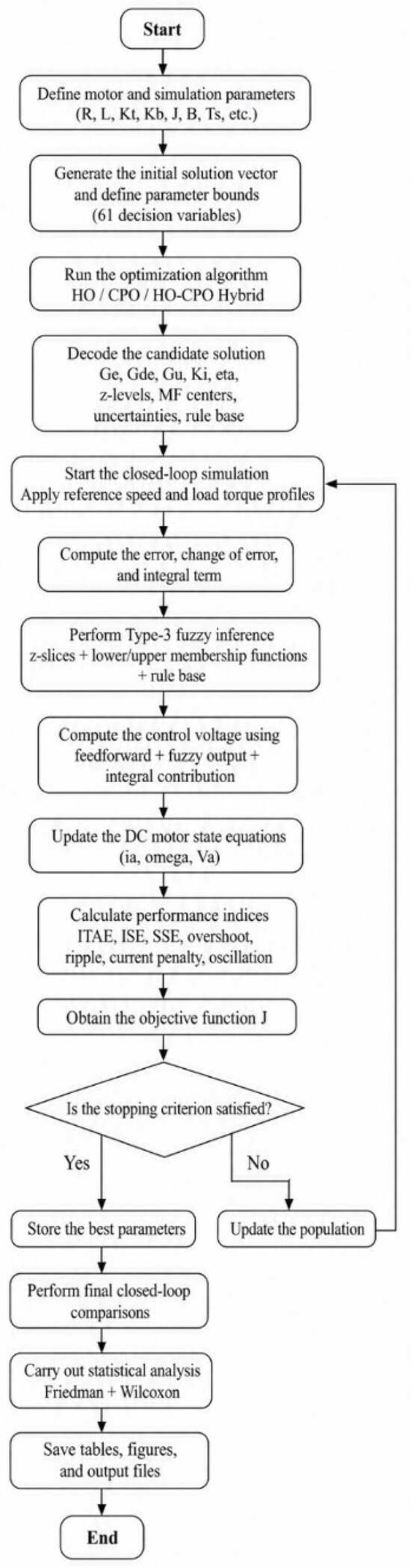
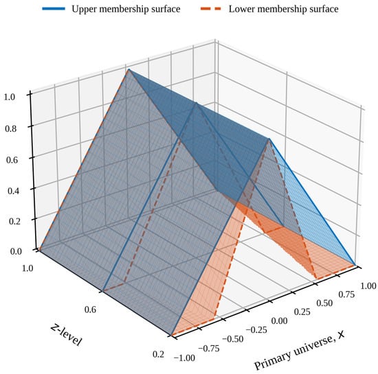
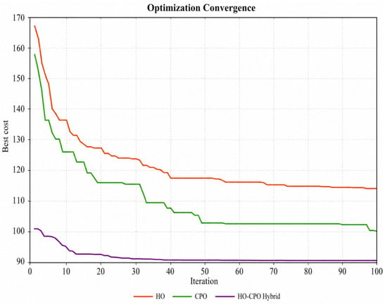
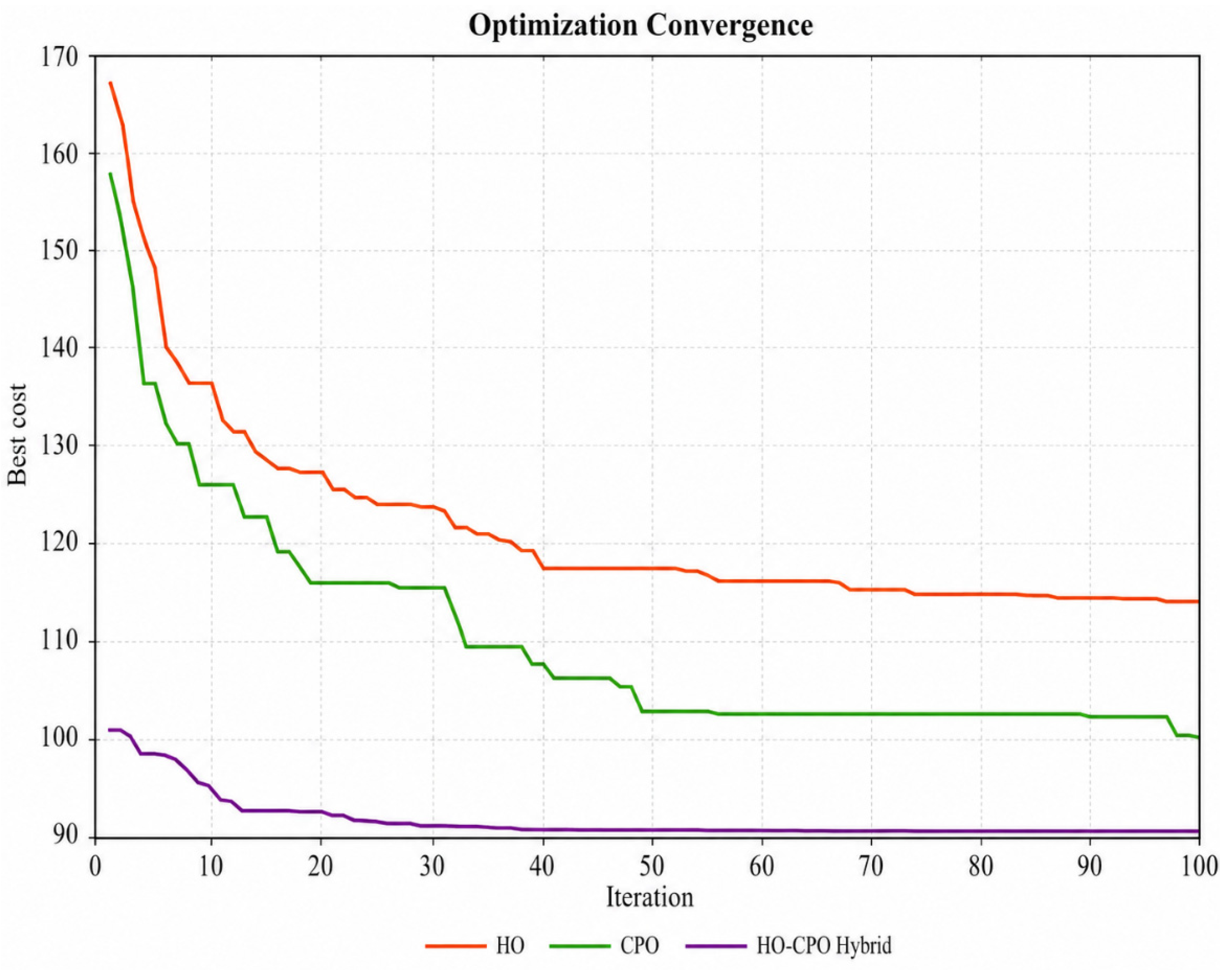
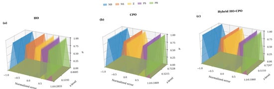
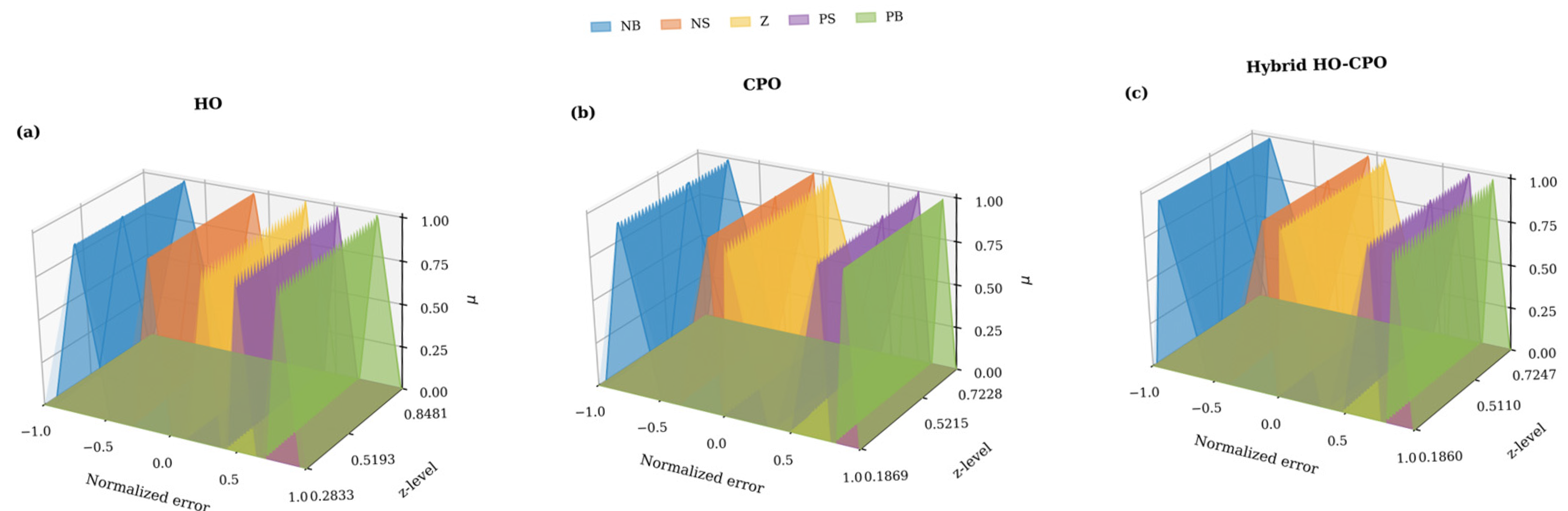
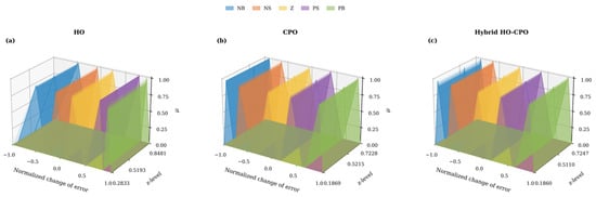
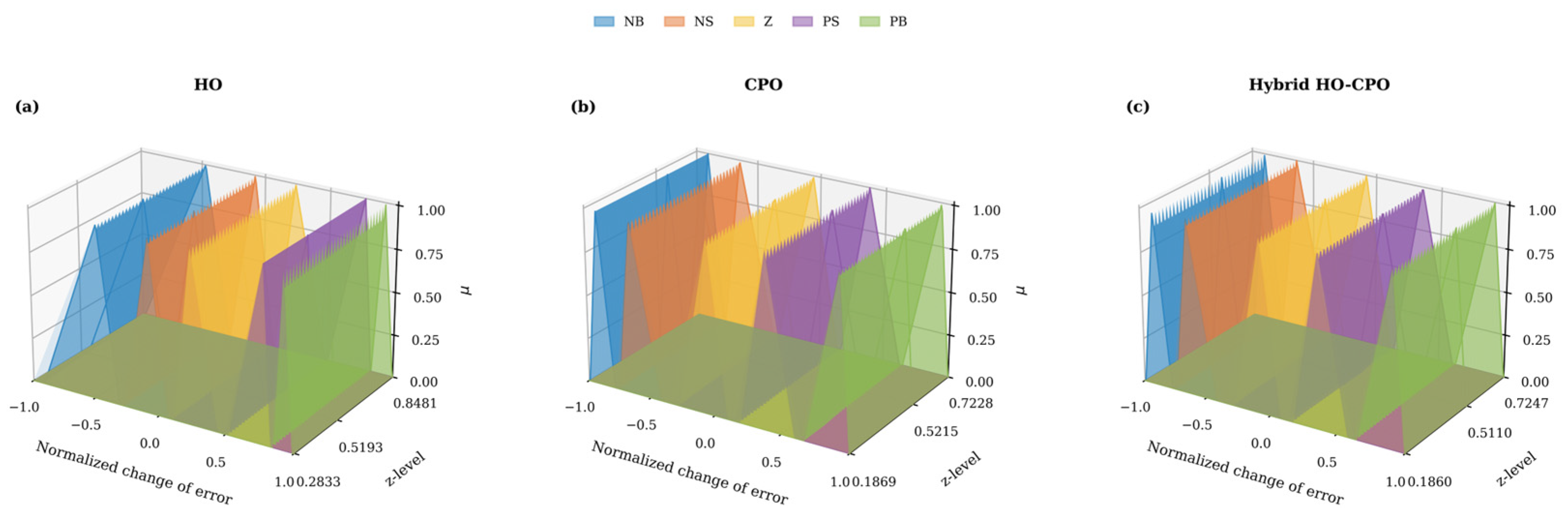
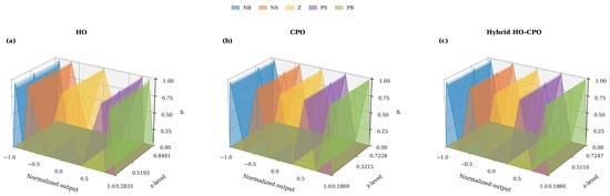
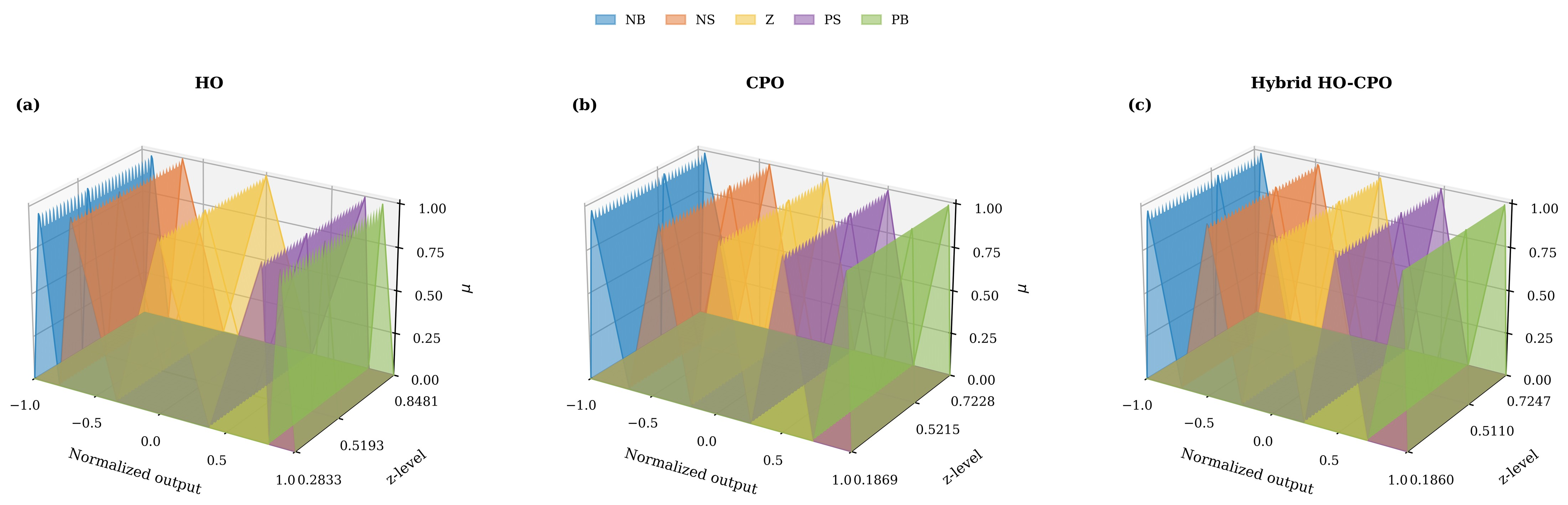
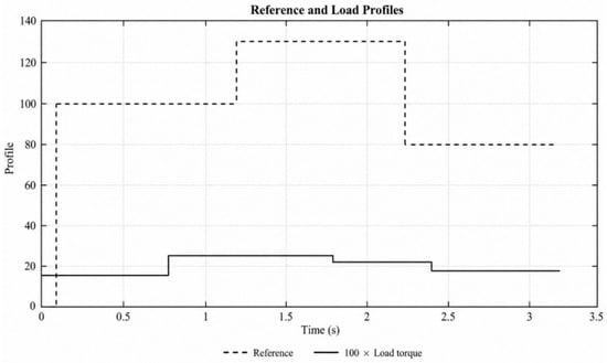
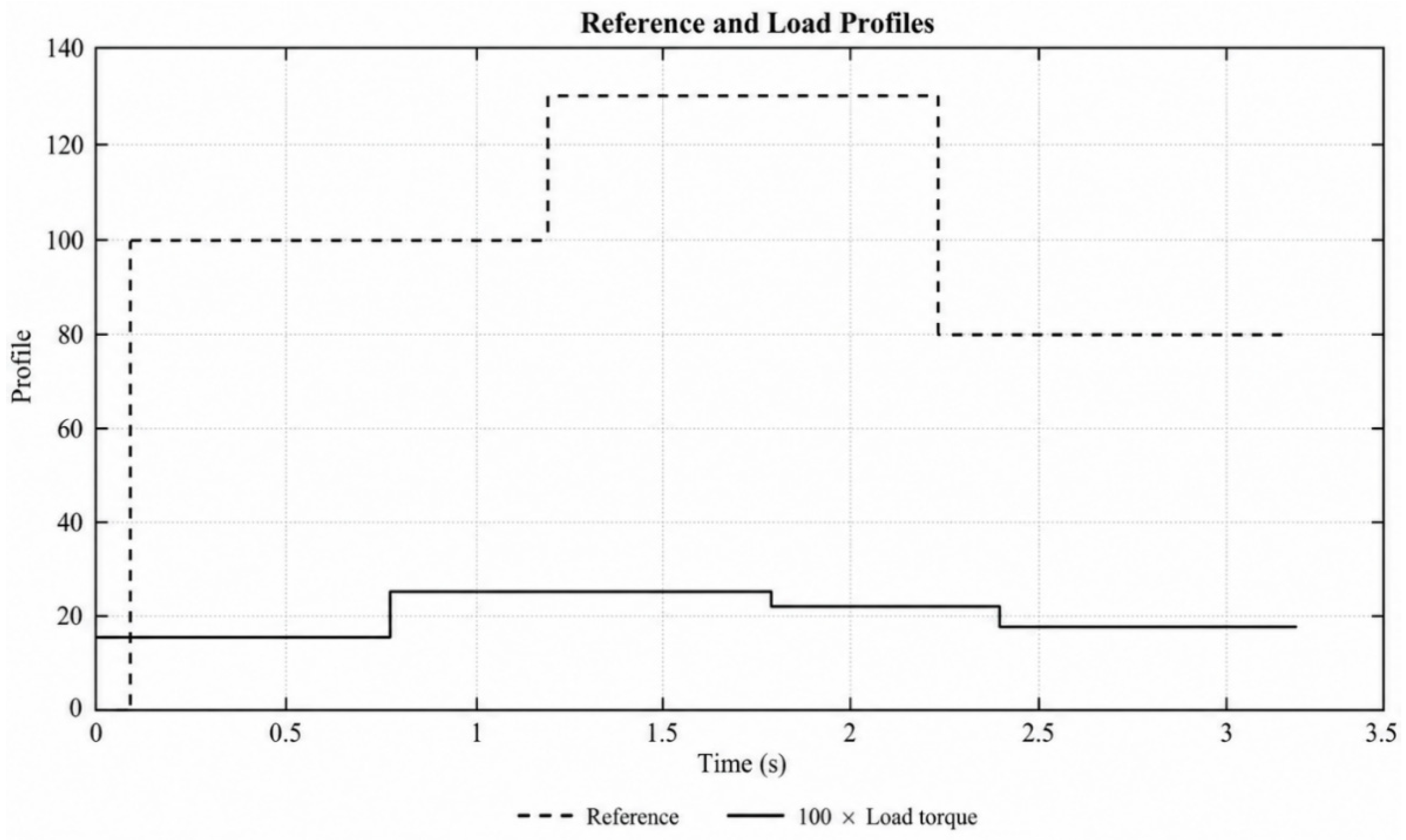
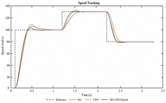
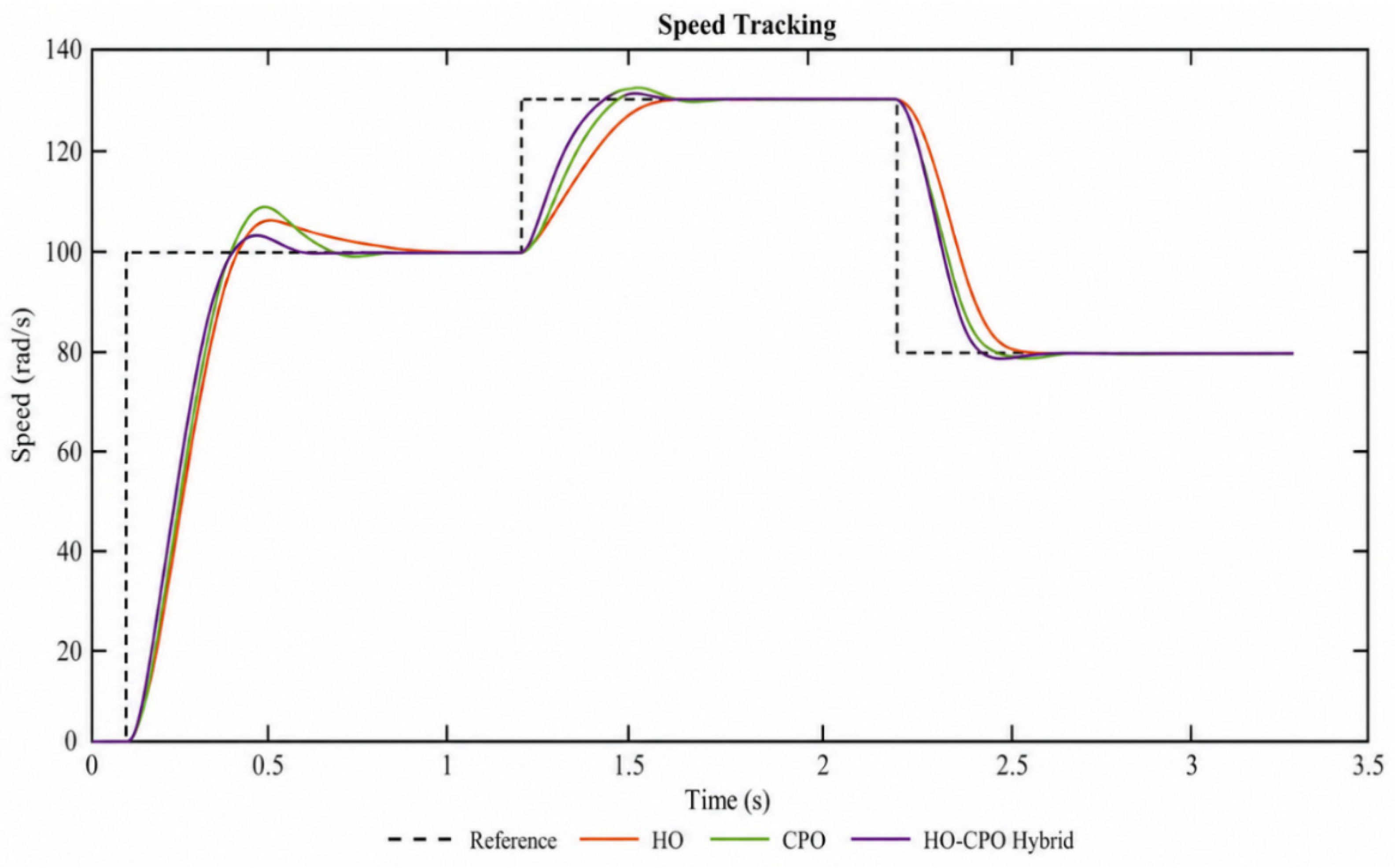
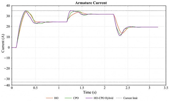
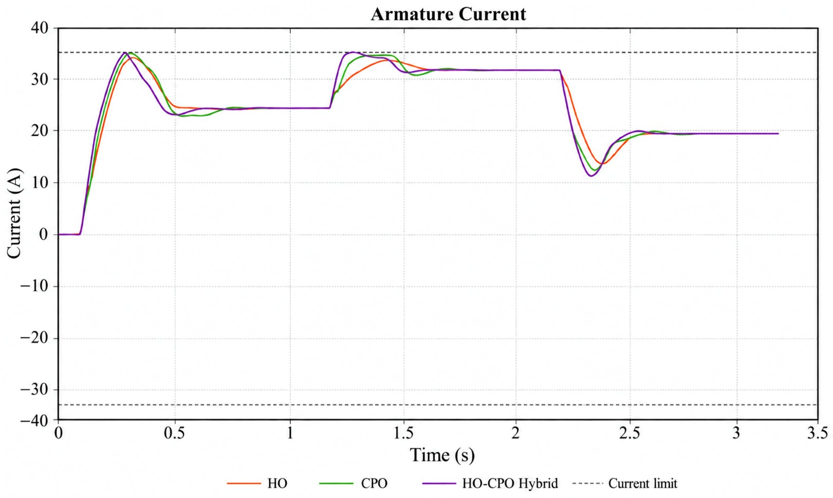
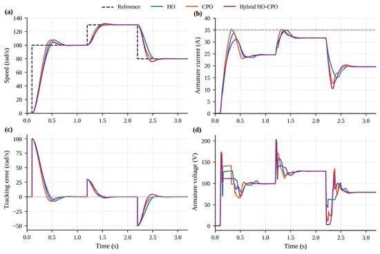
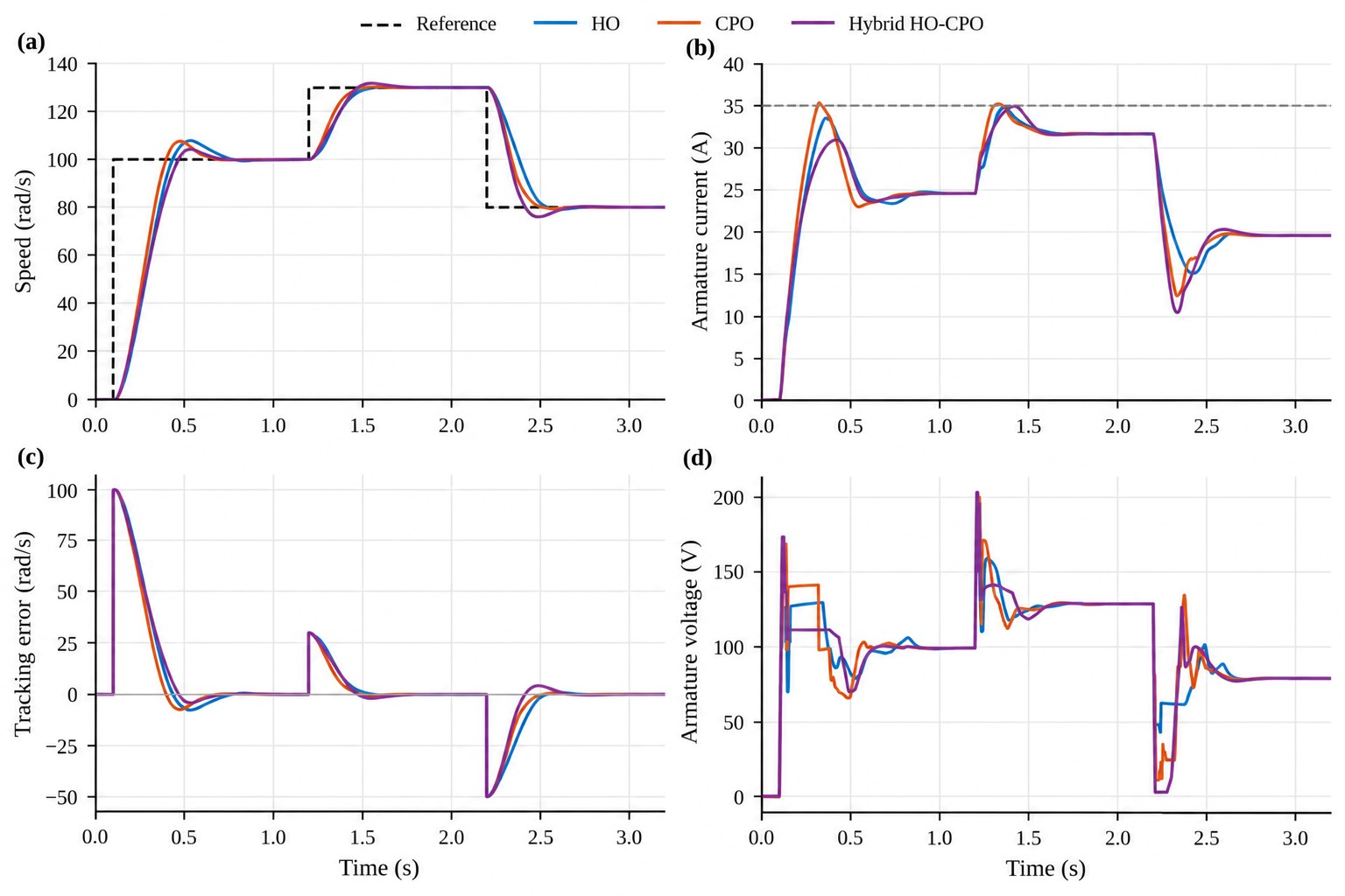
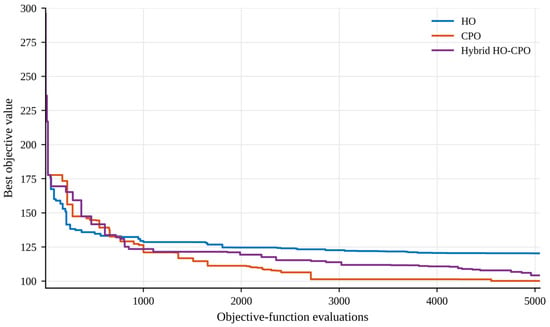
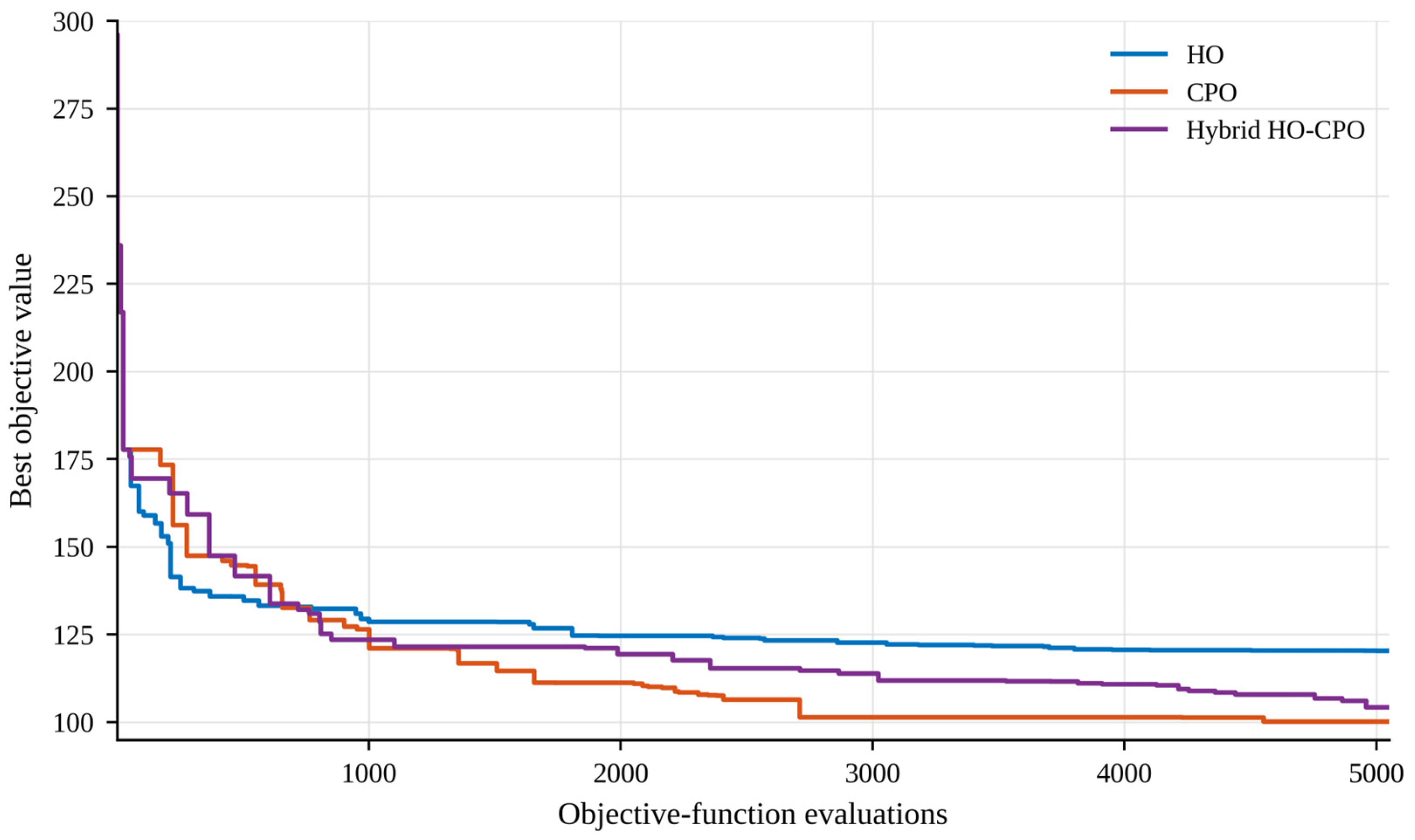
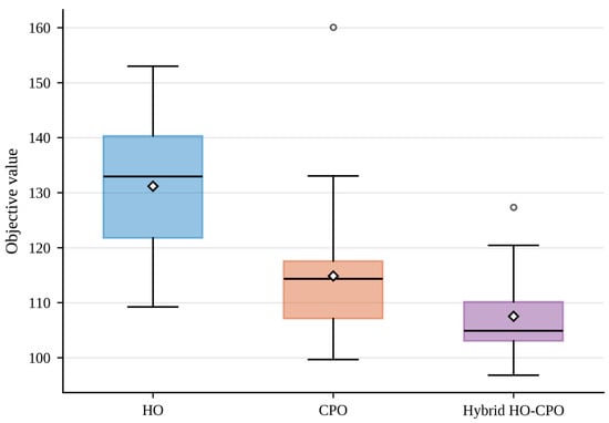
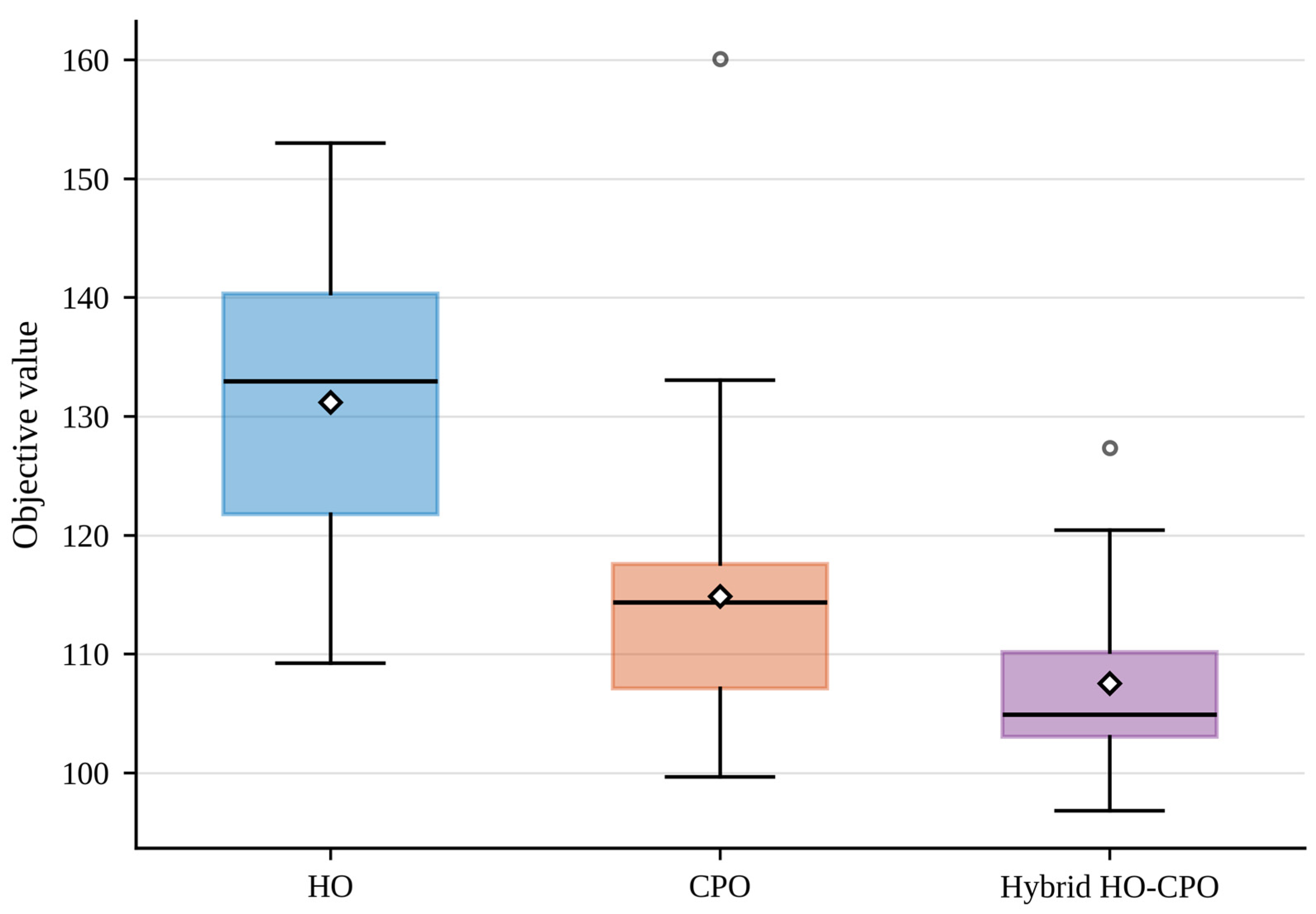
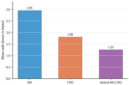
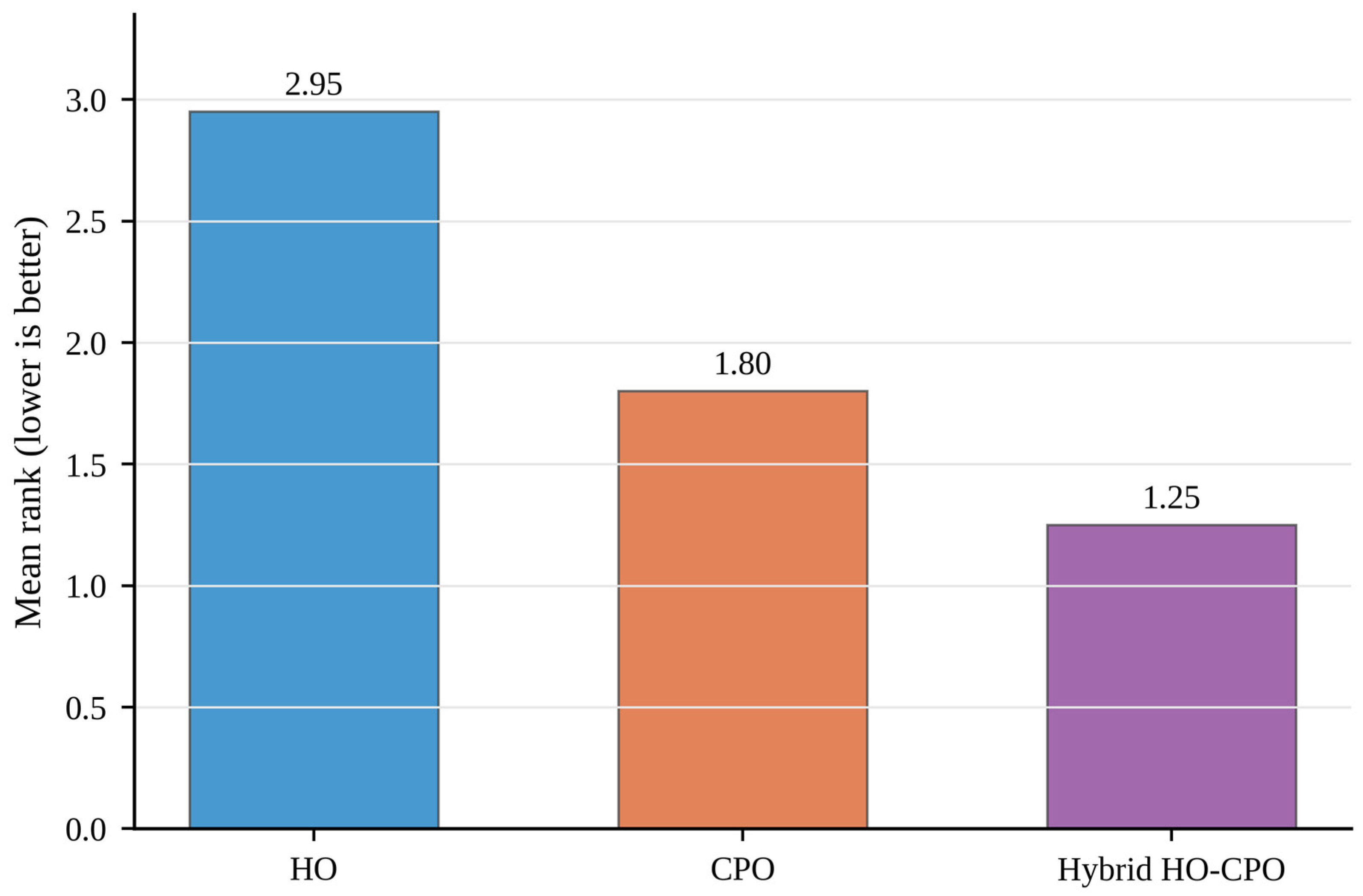
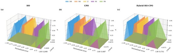
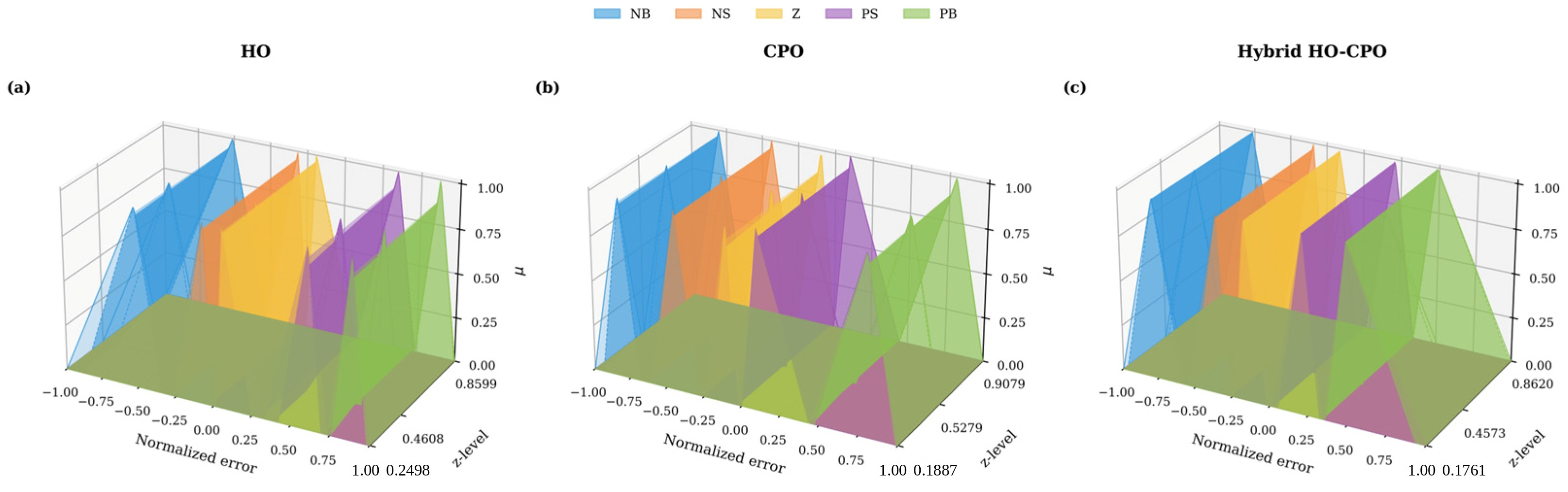
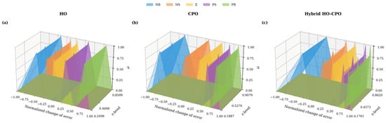
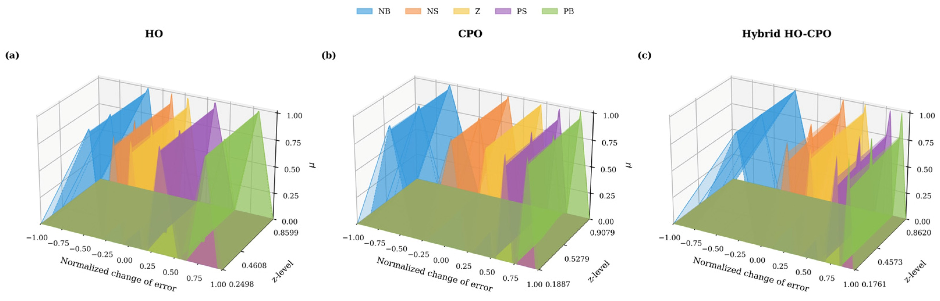
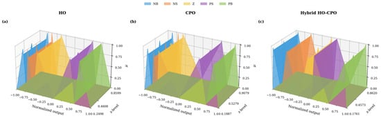
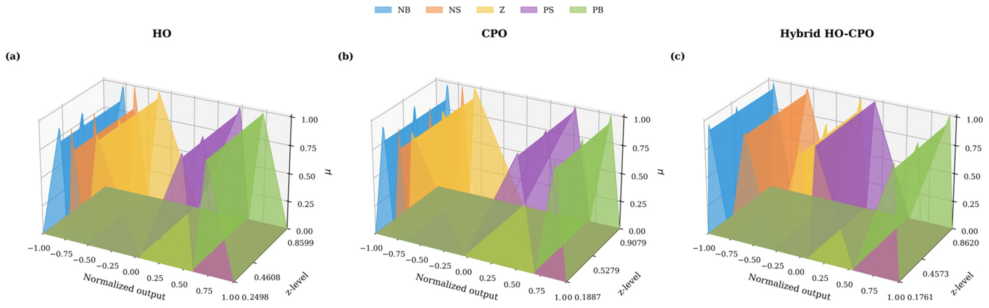
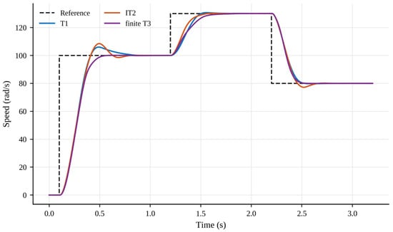
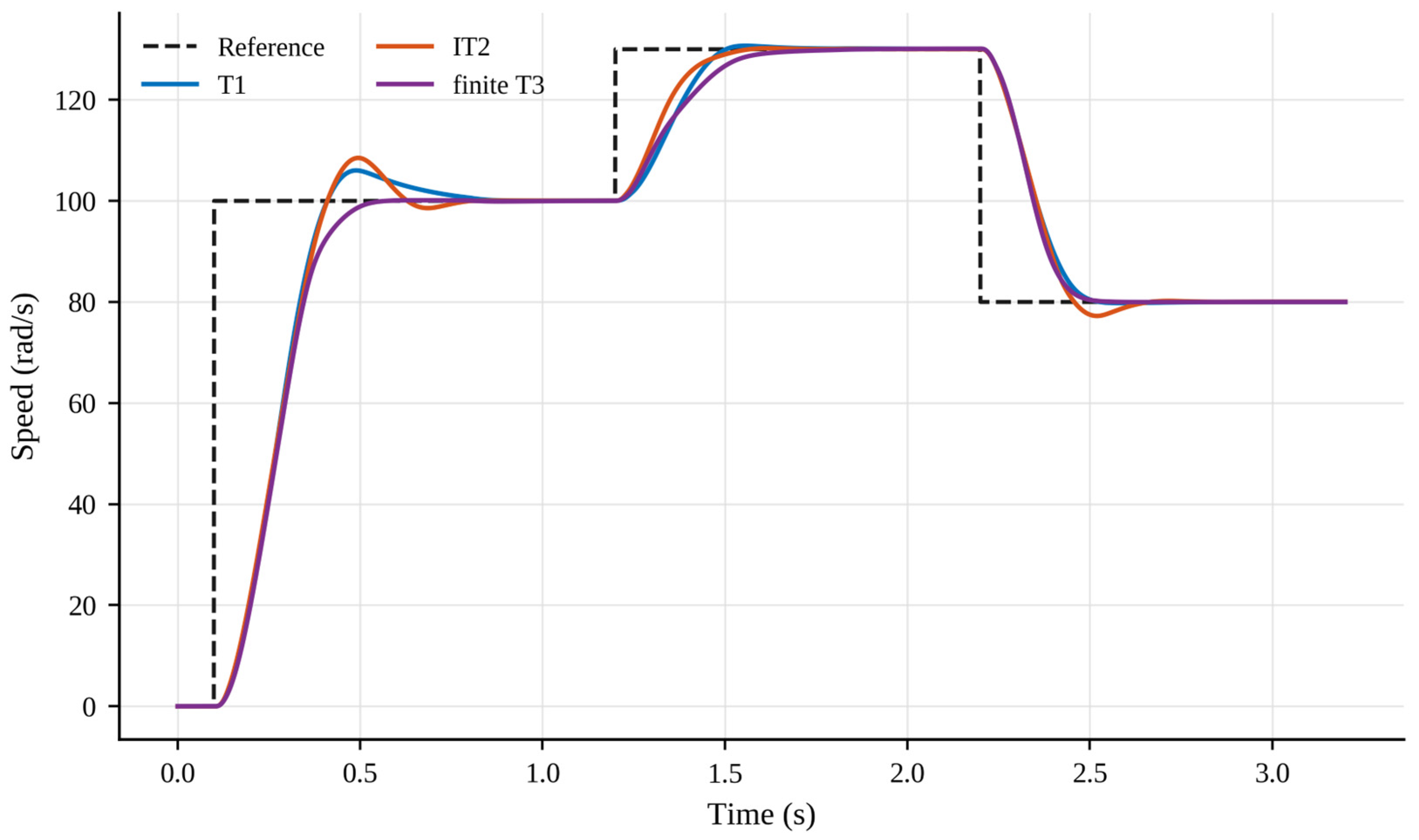
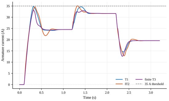
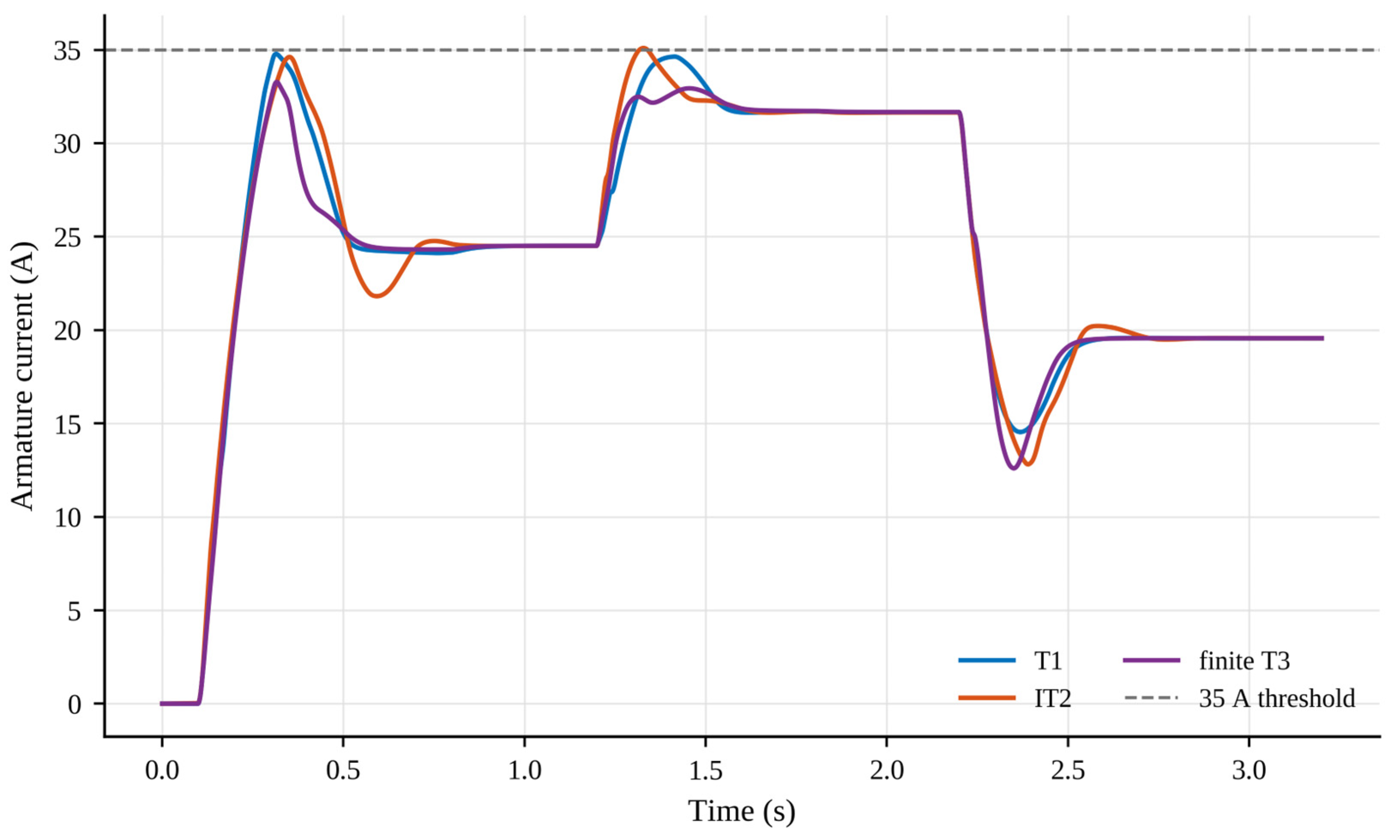
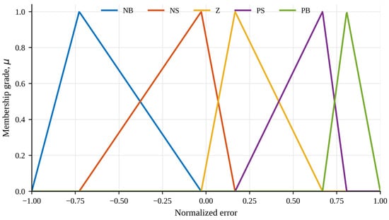
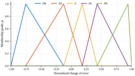
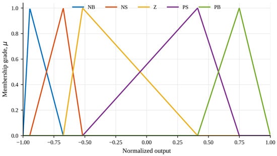
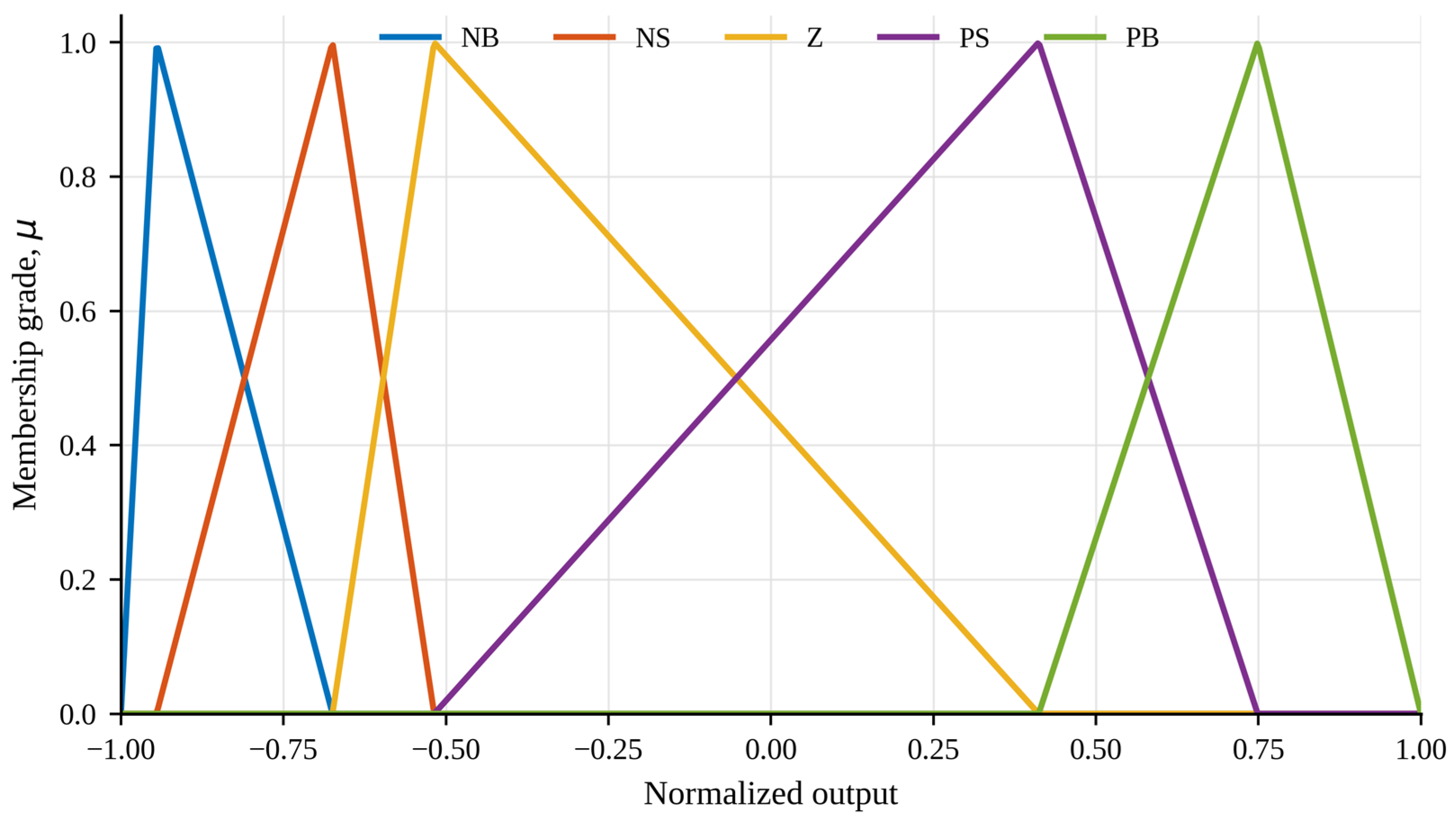
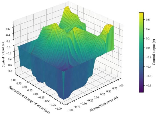
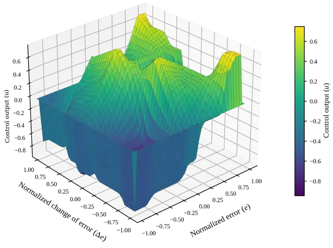
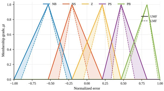
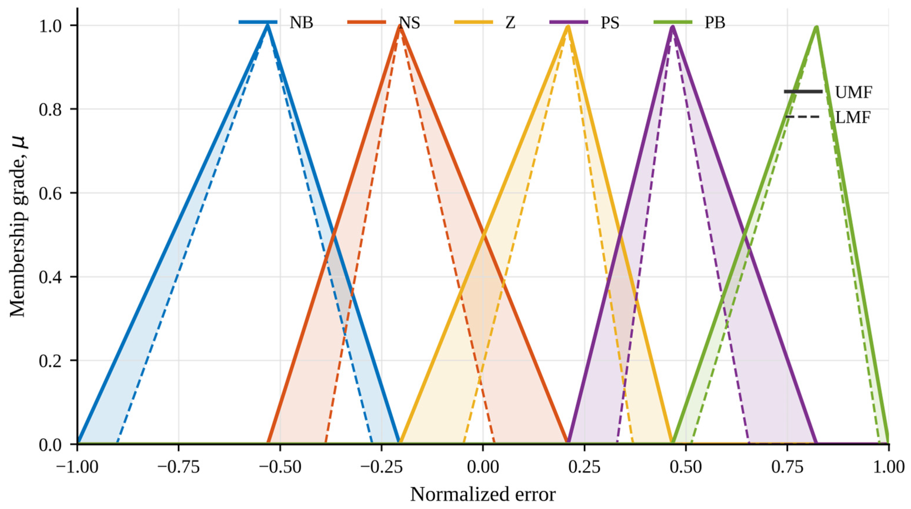
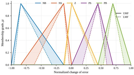
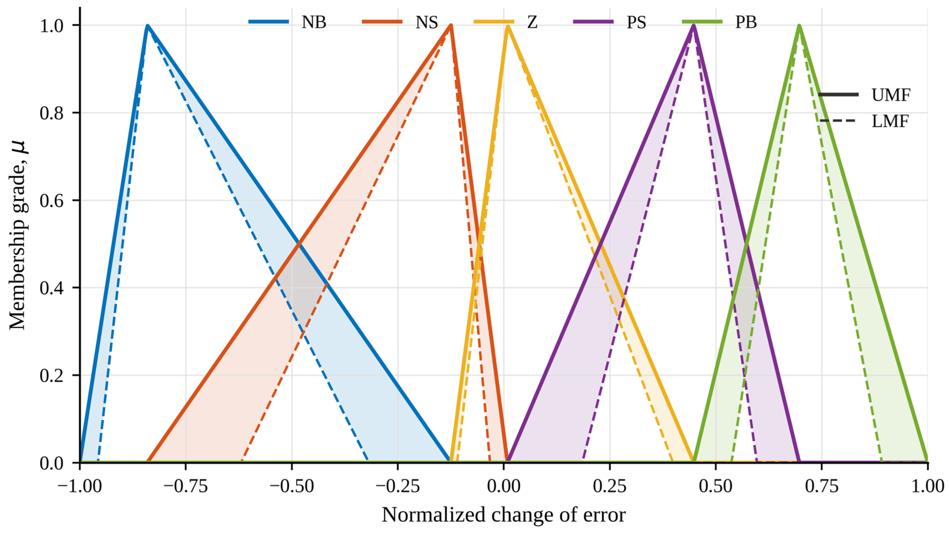
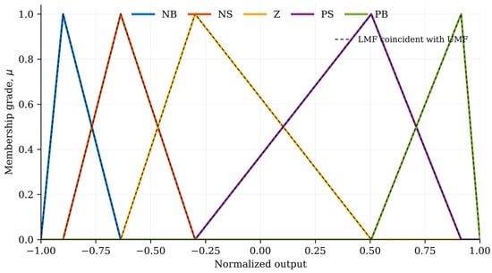
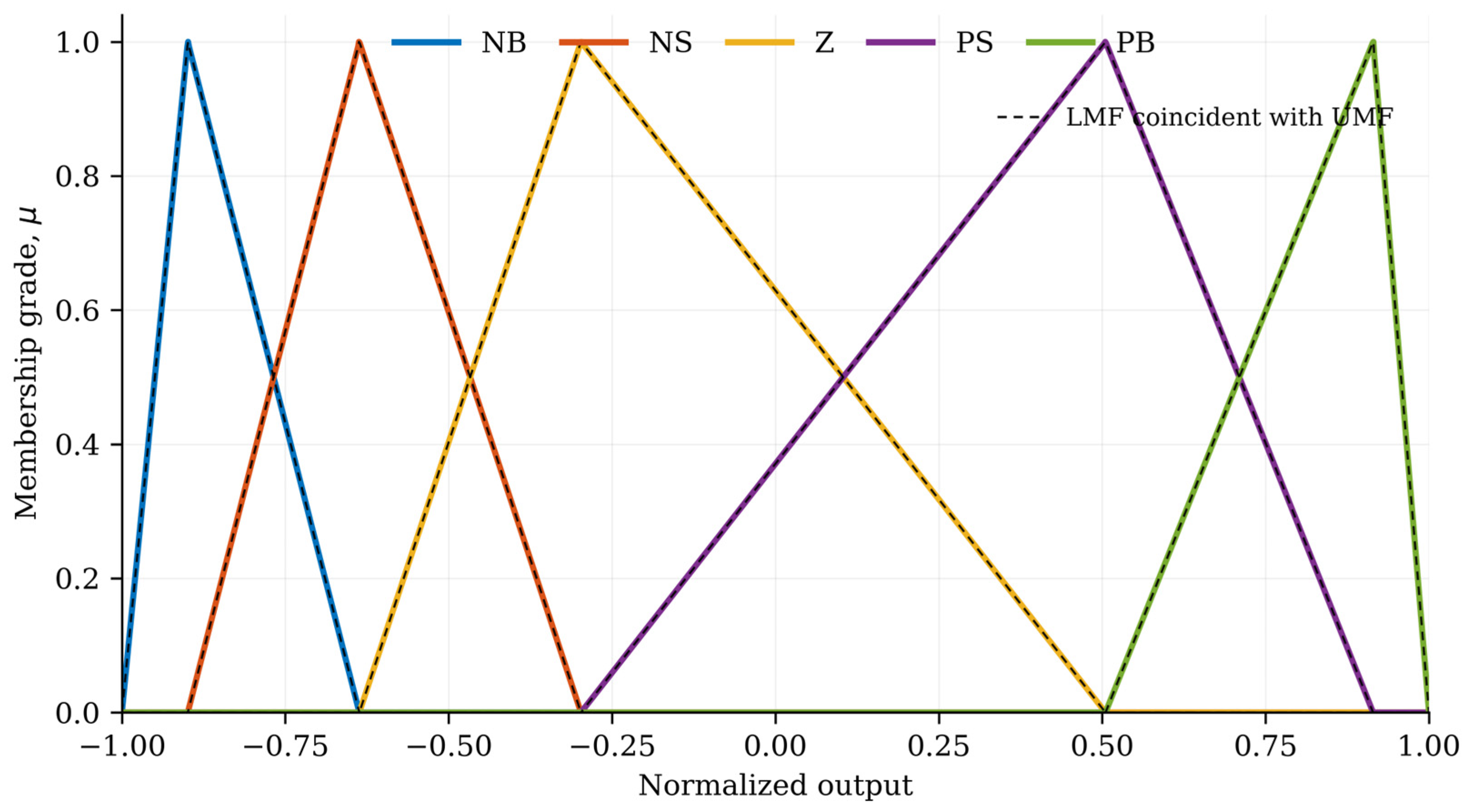
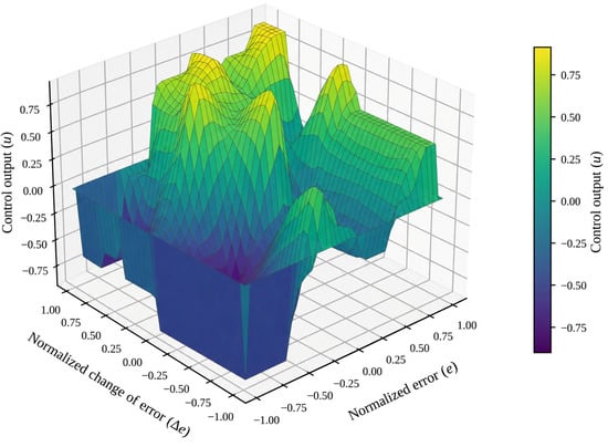
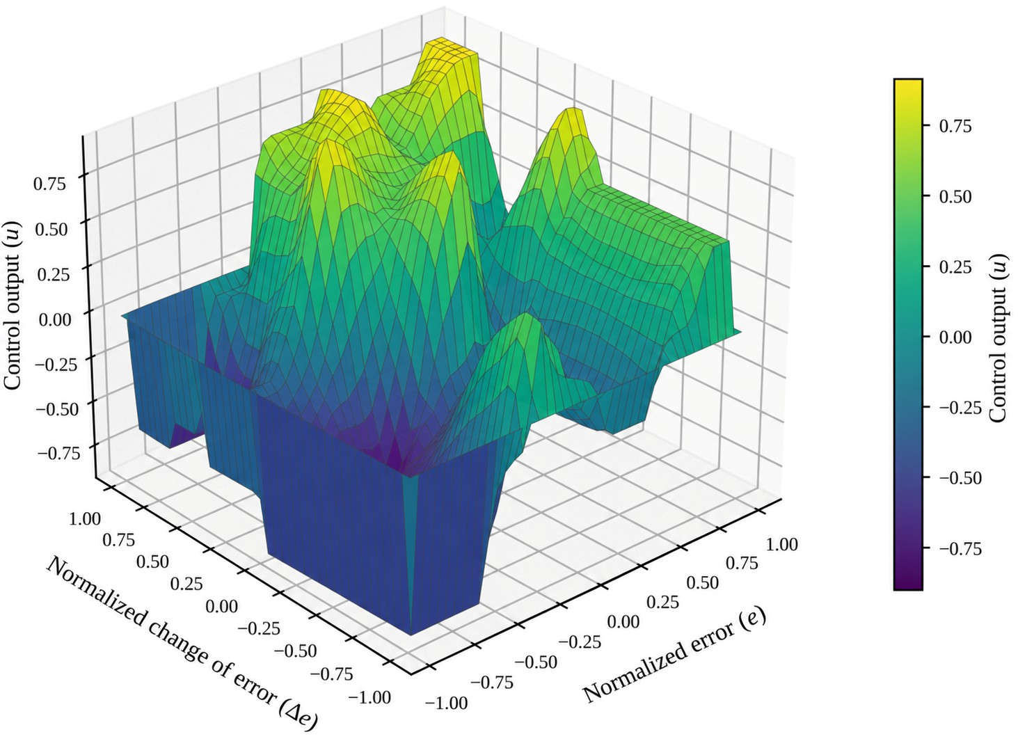
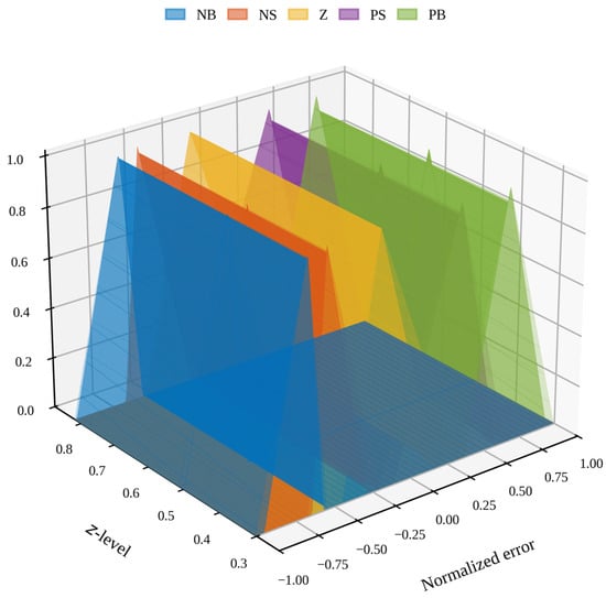
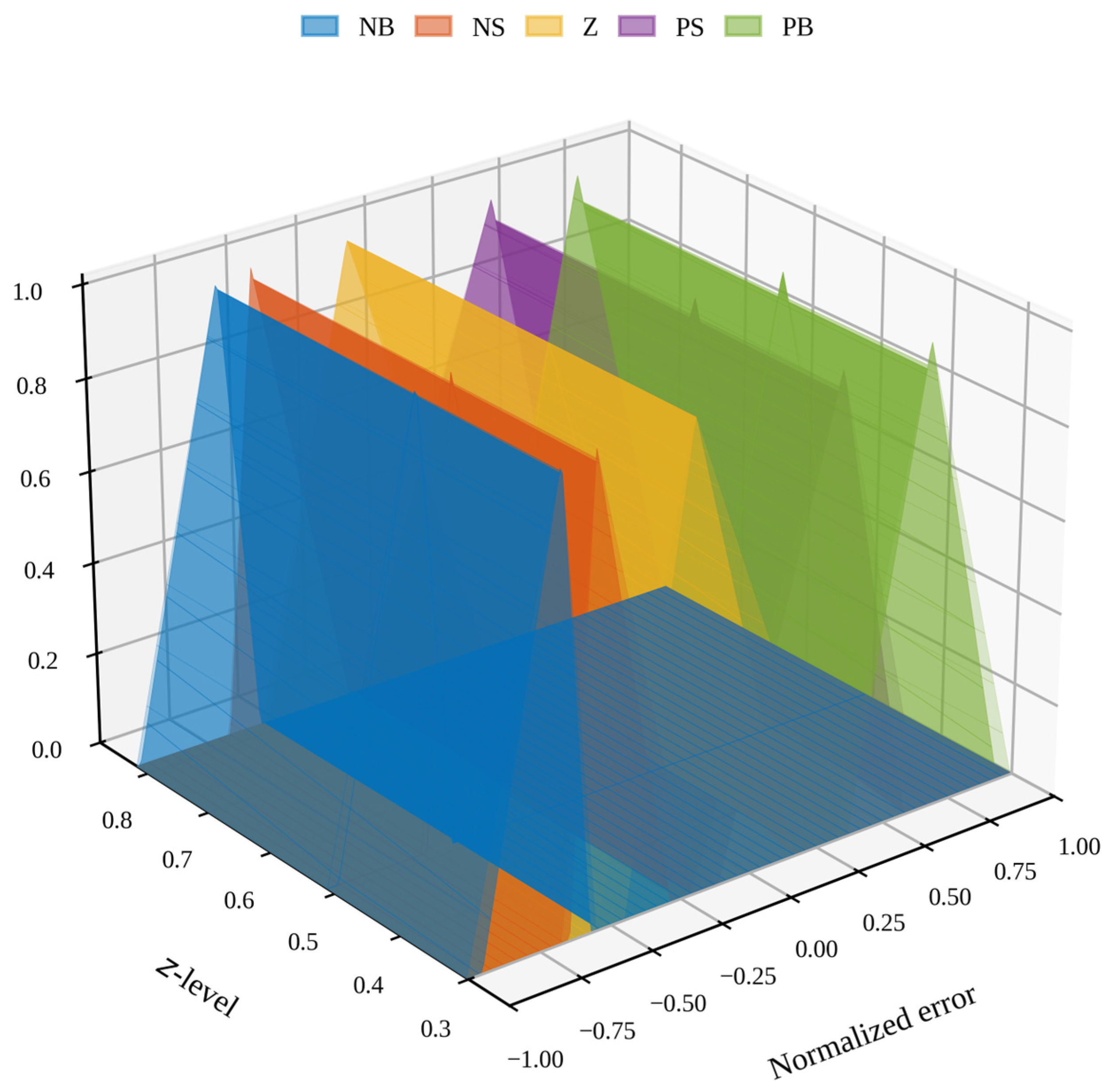
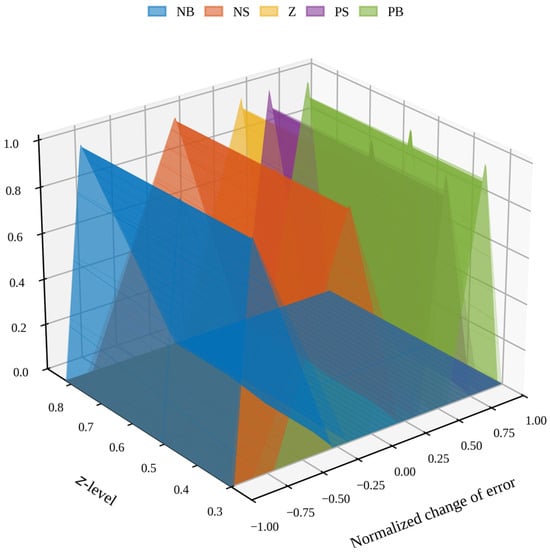
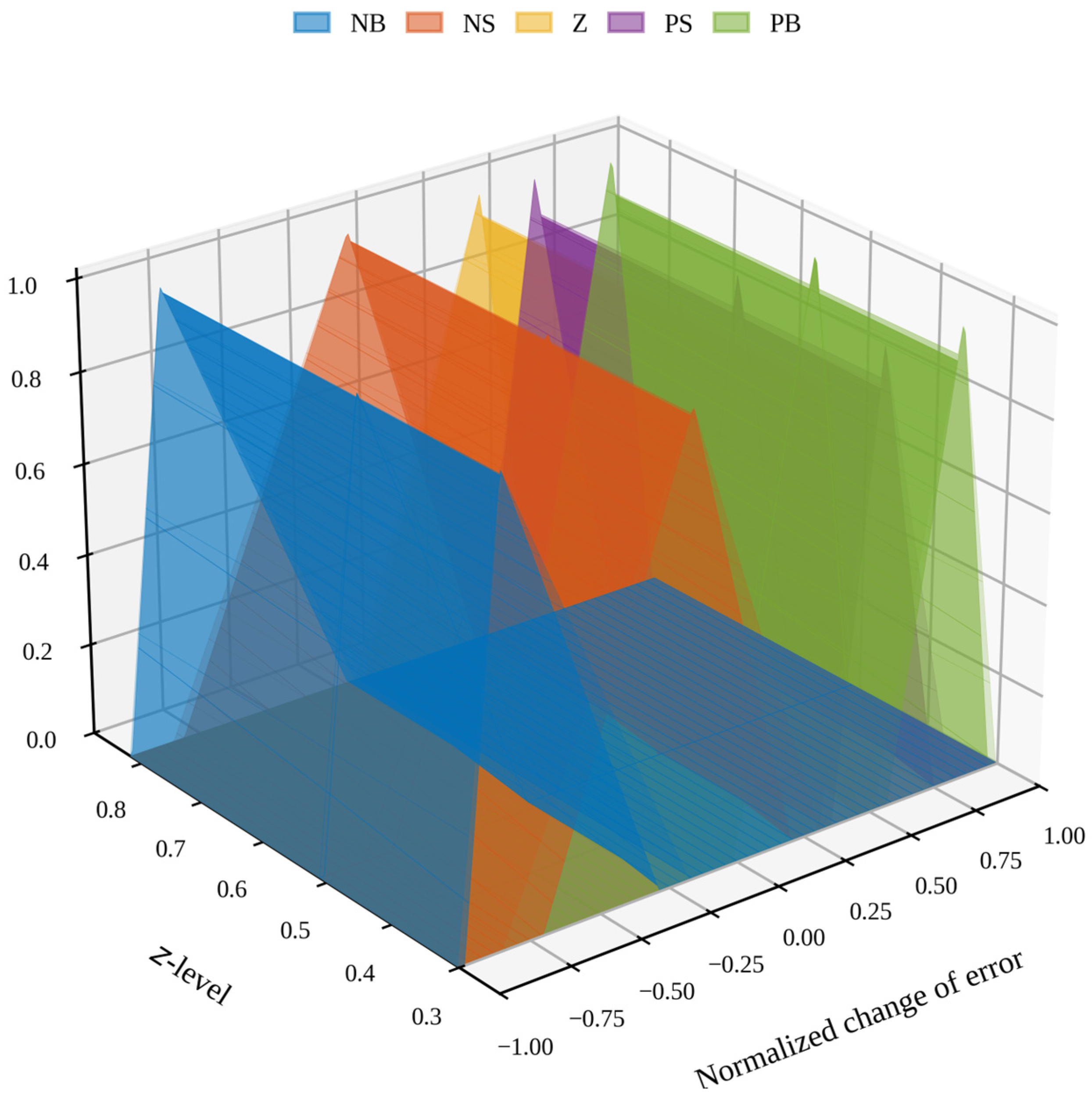
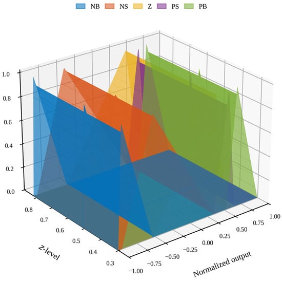
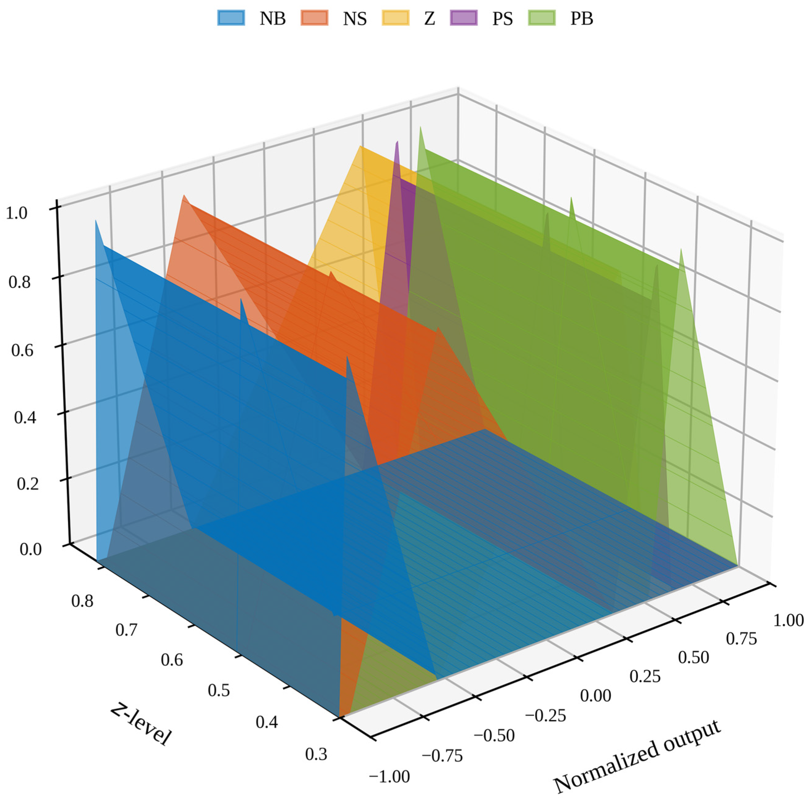
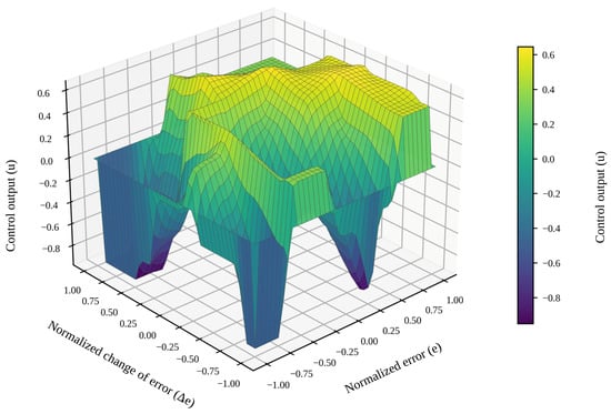
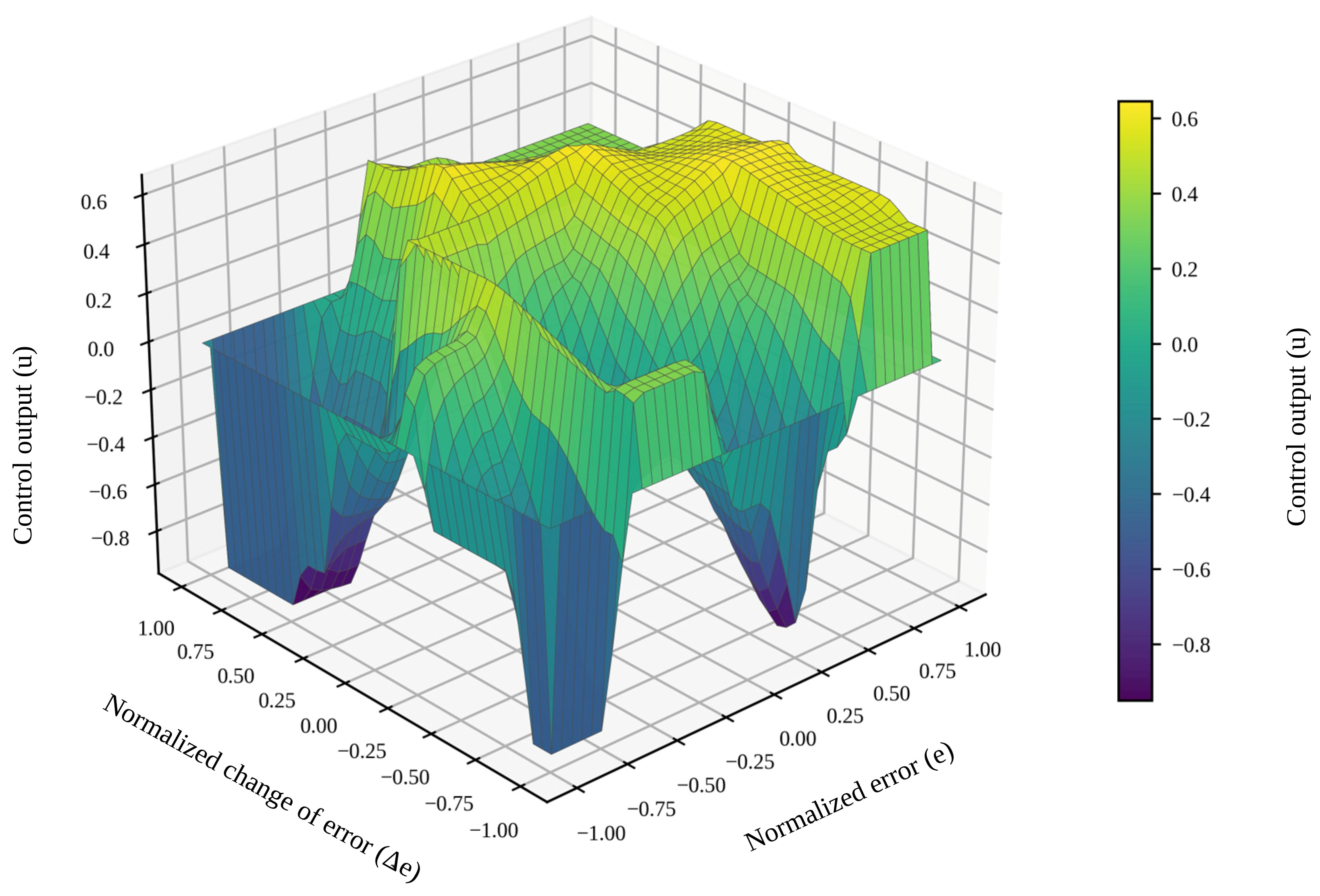
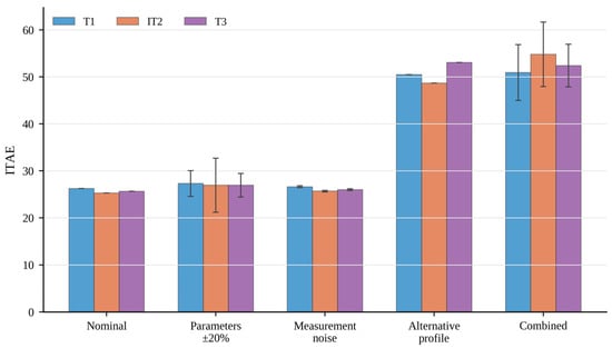
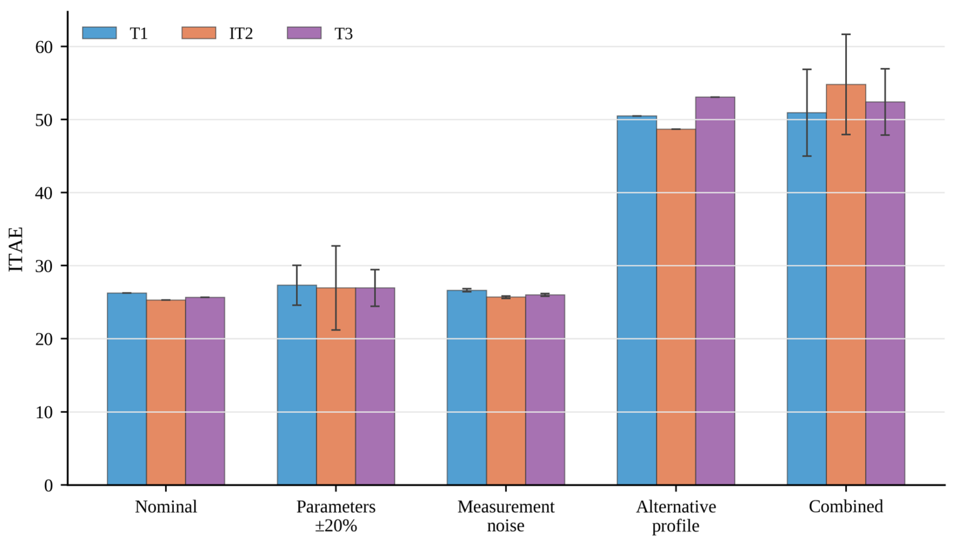
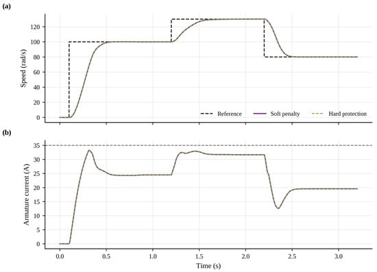
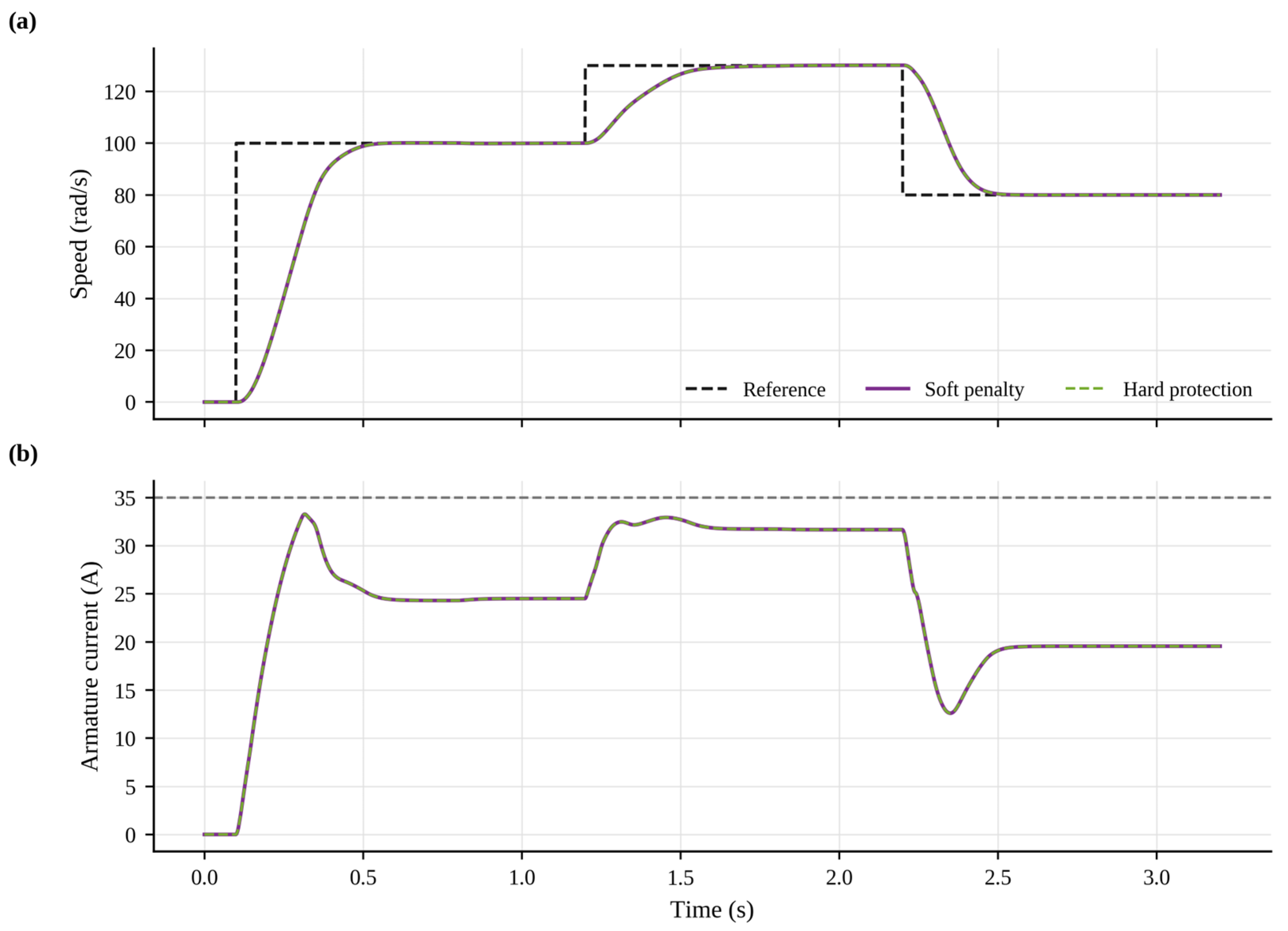
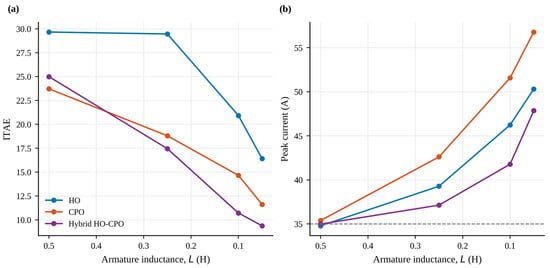
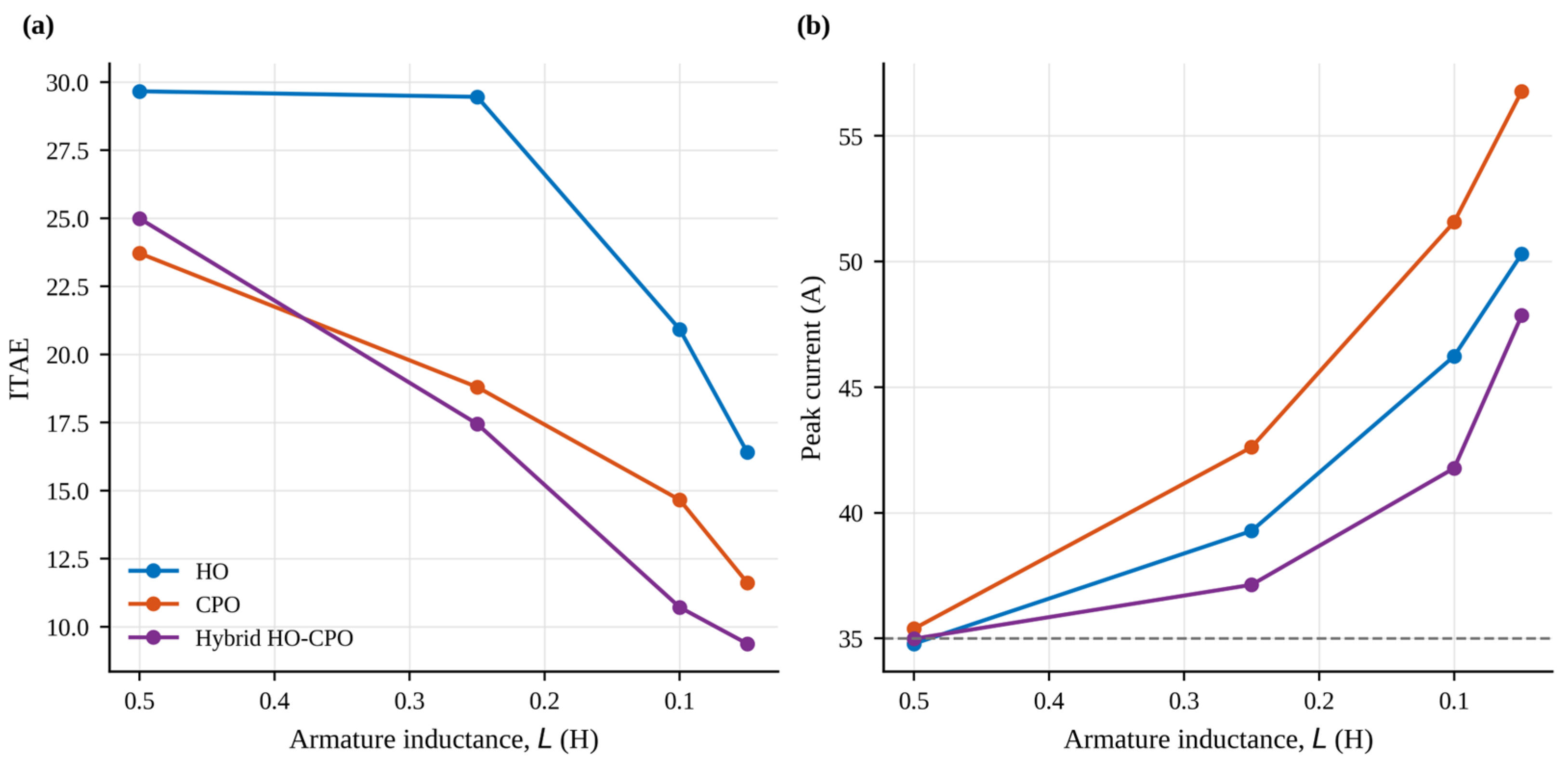
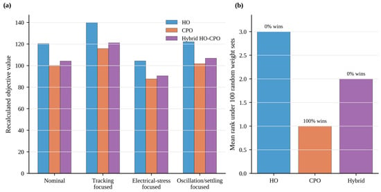
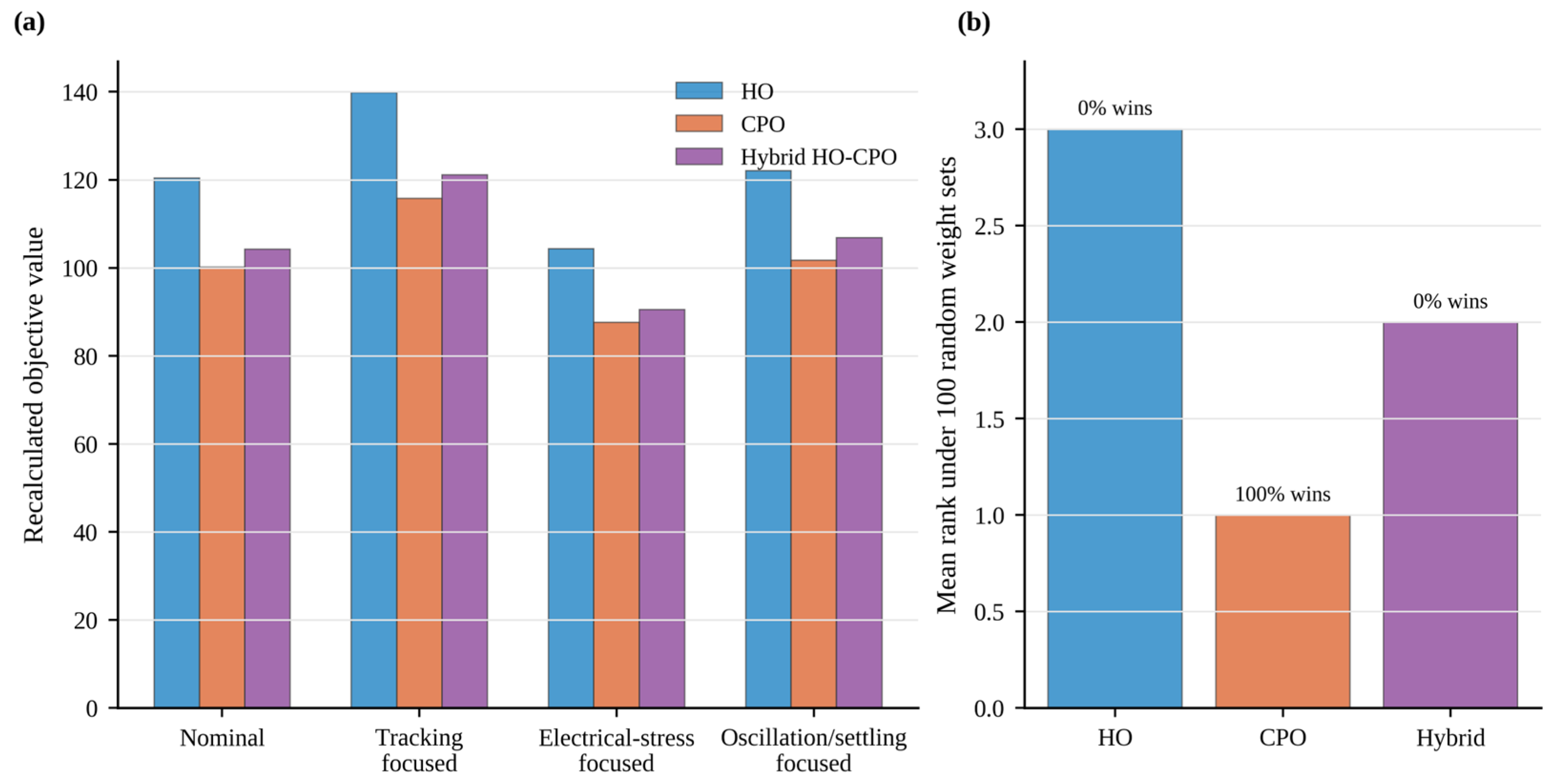
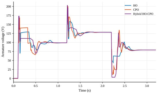
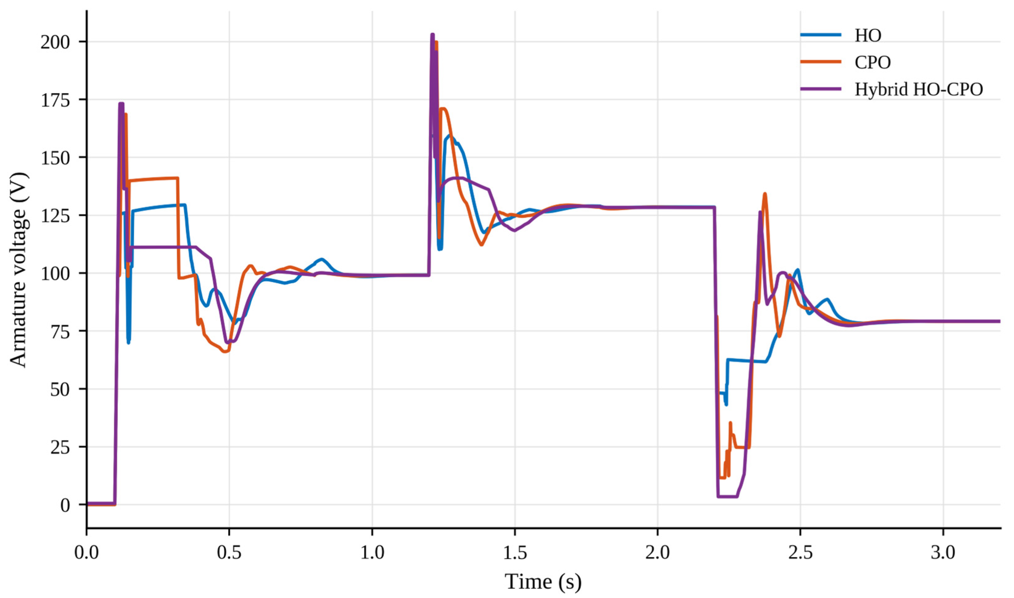

Disclaimer/Publisher’s Note: The statements, opinions and data contained in all publications are solely those of the individual author(s) and contributor(s) and not of MDPI and/or the editor(s). MDPI and/or the editor(s) disclaim responsibility for any injury to people or property resulting from any ideas, methods, instructions or products referred to in the content. |
© 2026 by the author. Licensee MDPI, Basel, Switzerland. This article is an open access article distributed under the terms and conditions of the Creative Commons Attribution (CC BY) license.