Coordinated Synchronous Condensers and Static Var Generator Planning Considering Unit Commitment-Dependent Multiple Renewable Energy Station Short-Circuit Ratio Constraints

Abstract

Ensuring adequate voltage support capability is a key challenge in planning power systems with large-scale renewable integration. This paper proposes a coordinated planning approach for synchronous condensers (SCs) and static var generators (SVGs) that accounts for unit commitment (UC)-dependent multiple renewable energy station short-circuit ratio (MRSCR) constraints. A UC–SC–SVG model is formulated to jointly determine SC and SVG siting and sizing, coordinating the short-circuit support of SCs with the reactive power regulation of SVGs. An impedance-aware graph residual network (IAGRN) is then developed to learn the nonlinear MRSCR residuals not captured by the first-order UC–SC physical model. Boundary-focused training and one-sided safety calibration are introduced to reduce the risk of misclassifying unsafe operating states as secure. The calibrated ReLU network is then converted into an equivalent mixed-integer linear representation and embedded in the planning model. Case studies on a provincial aggregated power system show that the proposed approach satisfies the MRSCR requirement across the representative operating states while achieving an economical allocation of SC and SVG capacity. Exact MRSCR post-checks and transient simulations further support the effectiveness of the embedded constraints and the voltage recovery performance of the resulting planning scheme.

1. Introduction

Driven by global decarbonization and energy transition targets, renewable energy capacity continues to expand rapidly. In 2025, newly installed solar photovoltaic (PV) and wind power capacity worldwide reached 510 GW and 159 GW, respectively, bringing their annual additions to a new record [1]. However, wind and PV plants are predominantly connected through power electronic converters and provide only limited short-circuit current under conventional grid following control [2,3]. As converter interfaced generation displaces part of the synchronous generation, particularly in large renewable energy bases connected through long-distance transmission corridors, the available short-circuit capacity and voltage support capability of the system may decline. The resulting weak grid conditions increase voltage sensitivity to power disturbances and may elevate the risks of transient overvoltage, converter instability, and cascading tripping of renewable plants following faults [2,3,4]. Maintaining sufficient grid strength under high renewable penetration has therefore become an important issue in power system planning.

Grid strength at a renewable point of interconnection (POI) can be characterized by the short-circuit ratio (SCR), which reflects the relationship between the available short-circuit capacity and the connected renewable capacity. However, conventional SCR evaluates each renewable plant independently and cannot adequately represent the electrical interactions among multiple closely coupled plants. Sun et al. [5] therefore proposed the multiple renewable energy station short-circuit ratio (MRSCR), in which the injections of neighboring renewable stations are converted to the target POI according to the ratios of mutual and self impedances. The resulting index relates the short-circuit capacity at each POI to the equivalent renewable injection affecting its voltage. Yuan et al. [6] extended generalized SCR-based small-signal stability assessment to multi-converter renewable systems containing static synchronous compensators, while Zhu et al. [7] proposed the impedance margin ratio to account more explicitly for the interactions between converter controls and network impedance. These studies also indicate that a scalar SCR-based index cannot represent all control-dependent dynamic phenomena. At the operational level, Lin et al. [4] incorporated MRSCR and short-term voltage security requirements into unit commitment, thereby linking unit commitment decisions to grid strength adequacy. A lower MRSCR generally corresponds to greater voltage sensitivity and weaker disturbance tolerance [4,5]. Because MRSCR depends on renewable injections and the network impedance matrix, it varies with transmission topology, online synchronous units, and SC installation. Therefore, there is an urgent need to incorporate operating state-dependent MRSCR constraints into power system planning.

Synchronous condensers (SCs) and static var generators (SVGs) provide complementary forms of voltage support in weak grids. An SC contributes short-circuit current and dynamic reactive power, thereby increasing the available short-circuit capacity and altering the equivalent network impedance observed from nearby renewable POIs [8,9]. In contrast, an SVG provides fast and continuously adjustable reactive power, but its converter-limited fault current capability does not offer the same synchronous short-circuit support as an SC [6]. Existing studies have mainly optimized SCs and SVGs along separate technical lines. Hadavi et al. [8] optimized SC locations and ratings by considering SCR requirements, voltage deviations, and equipment costs, and subsequently developed a mixed-integer convex formulation for SCR-constrained SC planning [9]. Wang et al. [10] transformed nonlinear SCR requirements in SC placement into mixed-integer linear constraints using Rayleigh cuts, whereas Fouladi et al. [11] formulated an SC siting and sizing model that additionally accounts for the fault current contribution of inverter-based resources. Lee et al. [12] optimized SC placement and voltage settings with respect to voltage and transient stability. Liang et al. [13] investigated a hybrid SC–SVG solution for a weak grid-connected wind farm and demonstrated the complementary voltage support characteristics of the two devices. Chu and Teng [14] further coordinated the planning of SCs and grid-forming inverter-based resources under small-signal stability and short-circuit current requirements. Nevertheless, these studies do not jointly determine SC and SVG locations and capacities while representing hourly variations in synchronous unit commitment. Accordingly, a unified multi-period planning framework is required to coordinate SC-based grid strength enhancement and SVG-based reactive power regulation across different operating states.

In addition to equipment allocation, hourly UC decisions alter the amount and spatial distribution of online synchronous support. Gu et al. [15] incorporated system strength and inertia requirements into generation dispatch, while Chu and Teng [16] formulated a short-circuit current constrained unit commitment model. Zhang et al. [17] extended this line of research by coordinating unit commitment and transmission switching under short-circuit current constraints, and Kim et al. [18] developed a strength-constrained unit commitment formulation for inverter-based resource-dominated systems. Together with the MRSCR-constrained unit commitment model in [4], these studies demonstrate the importance of representing grid strength as an operational constraint. However, incorporating the same dependence into equipment planning remains computationally demanding. Exact MRSCR evaluation requires reconstruction and inversion of the network admittance matrix for each combination of SC allocation and UC state. The resulting constraint contains nonlinear interactions among multiple SC installations, synchronous unit states, and renewable injections. Repeated exact evaluation is therefore difficult to integrate directly into a large-scale mixed-integer, multi-period planning model, whereas first-order approximations may lose accuracy when several planning and operating variables change simultaneously.

To address this computational challenge, machine learning-based surrogate models have been increasingly explored for tractable representation of complex power system security constraints. Data-driven security rule extraction has been applied to power system operation using stability rules [19] and sparse oblique decision trees [20]. Jia et al. further represented voltage security boundaries using ensemble sparse oblique regression trees and multiple learned convex constraints, and extended these methods to stability-constrained generation expansion planning [21,22,23]. Neural network surrogates have also been embedded in unit commitment models to approximate AC power flow equations and security criteria [24,25,26]. More recently, physics-informed graph neural networks have incorporated network topology and electrical relationships into optimal power flow learning [27,28]. Nevertheless, prediction accuracy alone does not guarantee the safety of an embedded surrogate. Formal verification and robustness studies have shown that neural networks may still produce physically inconsistent predictions or incorrectly classify unsafe operating points as secure within the admissible input domain [29,30]. Moreover, existing approaches do not directly provide an embeddable MRSCR representation that simultaneously captures impedance coupling, UC-dependent synchronous support, and nonlinear interactions among multiple SC installations. Therefore, an MRSCR surrogate for planning should combine a physical baseline with nonlinear residual learning, explicitly control false safe predictions near the security threshold, and remain compatible with mixed-integer optimization.

To address these issues, this paper proposes a coordinated SC–SVG planning method considering UC-dependent MRSCR constraints. The main contributions are summarized as follows:

1. A multi-period SC–SVG coordinated planning model with endogenous UC is formulated to jointly optimize the locations and capacities of SCs and SVGs together with hourly unit commitment and dispatch. SC installation and online synchronous units are explicitly represented in the network impedance and MRSCR evaluation, while SVGs provide adjustable reactive power support. An electrical candidate bus screening procedure with bounded refresh is employed to define a tractable siting domain.

2. An impedance-aware graph residual network (IAGRN) is developed to construct an embeddable UC-dependent MRSCR constraint. A first-order UC–SC physical model captures the principal variation in the MRSCR deficit, and the graph network learns the remaining nonlinear effects from exact impedance-based labels. Boundary-weighted fitting, unsafe underestimation penalization, monotonicity regularization, and one-sided calibration are introduced to improve prediction reliability near the security threshold. The calibrated ReLU network is subsequently reformulated as mixed-integer linear constraints and embedded in the planning model.

3. Case studies are conducted on a provincial aggregated power system under multiple representative operating scenarios. The proposed method is evaluated in terms of equipment allocation, planning economy, MRSCR security, surrogate accuracy, and transient voltage performance. Comparisons among different planning schemes and MRSCR formulations show that the proposed method achieves a better balance between planning economy and grid strength security. The planning results are further assessed through exact simplified and full complex MRSCR calculations and transient voltage simulations.

2. Structure and SC–SVG Coordinated Planning Model Considering Unit Commitment

For the coordinated planning of SCs and SVGs under UC-dependent MRSCR requirements, Section 2 presents the overall framework and formulates the original planning model with hourly UC decisions.

2.1. Structure Framework

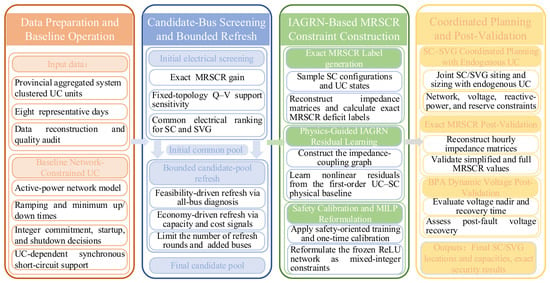
Figure 1 illustrates the overall framework of the proposed SC–SVG coordinated planning method considering UC-dependent MRSCR constraints. The proposed framework begins with a network-constrained UC problem solved for the provincial aggregated system over eight representative days to obtain baseline hourly commitment states for candidate screening and dataset construction. A common candidate pool for SCs and SVGs is then established based on the MRSCR improvement provided by SC installations and the Q–V support sensitivities of candidate buses, with bounded pool refresh applied when necessary. Subsequently, short-circuit impedance matrices are reconstructed under sampled SC configurations and UC states to generate exact MRSCR labels. The IAGRN is trained to learn the nonlinear residuals relative to the first-order UC–SC physical model, followed by one-sided safety calibration and mixed-integer linear reformulation. The resulting calibrated MRSCR constraints are embedded in the coordinated planning model, where SC and SVG siting and sizing are jointly optimized together with hourly UC and system operation. Finally, the obtained planning solution is post-validated through exact impedance matrix reconstruction and further evaluated by transient simulations of post-fault voltage recovery.

Figure 1. The overall framework of the proposed SC–SVG coordinated planning method considering UC-dependent MRSCR constraints.

2.2. Candidate Bus Screening and Bounded Pool Refresh

To reduce the equipment siting search space and the number of candidate nodes included in the IAGRN, a common electrical candidate pool is established for SCs and SVGs before dataset construction and planning optimization. The screening combines an MRSCR deficit reduction index with a Q–V voltage support index.

The MRSCR-based index measures the reduction in the MRSCR deficit obtained from a one-module SC perturbation. Let $M_{r,s}^0$ denote the MRSCR at renewable POI r under state s without the candidate SC module, and let $M_{r,s}^i$ denote the corresponding value obtained by connecting one SC module at bus i and reconstructing the short-circuit impedance matrix. The MRSCR-based index is defined by Equation (1):

$${\phi }_i={\displaystyle \sum _{s\in \mathcal{S}}{\displaystyle \sum _{r\in \mathcal{R}}\left({\left[{\gamma }^{\min }-M_{r,s}^0\right]}_{+}-{\left[{\gamma }^{\min }-M_{r,s}^i\right]}_{+}\right)}}$$

(1)

where $ℛ$ is the set of renewable POIs, γ^min is the prescribed MRSCR threshold, and [x]₊ = max(x,0). A larger φ_i corresponds to a greater reduction in the aggregate MRSCR deficit. Ties are resolved sequentially using the mean increase in the system minimum MRSCR and the mean increase over all renewable POIs.

The Q–V sensitivity is calculated from the reduced coefficient matrix of the state-independent linear P–Q–V–θ power flow model in [31]. For each non-slack candidate bus i, a balanced perturbation is specified by ΔQ_i = 1 Mvar, ΔQ₀ = −1 Mvar, and ΔP = 0. The resulting sensitivity is defined by Equation (2):

$${\chi }_{\mathit{ki}}={\displaystyle \frac{\Delta V_k}{\Delta Q_i}},$$

(2)

where χ_ki is the voltage sensitivity of bus k with respect to reactive power injection at bus i. Under the fixed topology screening model, the coefficient matrix and the resulting Q–V sensitivities are held constant across UC states. These sensitivities are used only for initial candidate screening, whereas the effect of SC installation on the short-circuit impedance matrix is explicitly represented in the subsequent MRSCR evaluation. The voltage support index aggregates the positive voltage responses at renewable POIs and buses with high reactive power demand, as expressed in Equation (3):

$${\Psi }_i=\alpha {\displaystyle \sum _{r\in \mathcal{R}}{a}_r}{\left[{\chi }_{\mathit{ri}}\right]}_{+}+\left(1-\alpha \right){\displaystyle \sum _{k\in \mathcal{L}}{b}_k}{\left[{\chi }_{\mathit{ki}}\right]}_{+},$$

(3)

where $ℒ$ is the set of buses with high positive reactive power demand; a_r and b_k are normalized weights proportional to renewable capacity and reactive power demand, respectively; and α specifies the relative weight of the two target groups. After separate normalization, the two indices are combined according to Equation (4).

$${\eta }_i=\beta {\phi }_i^n+\left(1-\beta \right){\Psi }_i^n,$$

(4)

where ${\phi }_i^n$ and ${\Psi }_i^n$ are the normalized non-negative parts of φ_i and Ψ_i, respectively, and β is the weighting coefficient. For a prescribed even pool size K, the highest ranked K/2 buses under each individual index are retained. If these subsets overlap, the remaining positions are assigned in descending order of η_i. The resulting set defines the common electrical candidate pool for SCs and SVGs.

The initial pool size is selected from a prescribed sequence using the linearized network model in [31]. For each K, the shortlisted buses are assigned their maximum admissible SC and SVG capacities, and feasibility is checked at the peak load hour of each representative day under the baseline UC states. The candidate pool is expanded if the restricted siting domain causes infeasibility or excludes a lower cost all-bus solution. The corresponding external buses identified by the all-bus diagnostic are then appended. After a bounded number of refreshes, the candidate pool is fixed for IAGRN dataset construction and final planning.

2.3. SC–SVG Coordinated Planning Model with Endogenous UC

Based on the framework described above, the SC–SVG coordinated planning model with endogenous UC is formulated as follows.

2.3.1. Objective Function

The objective is to minimize the total annual cost, including the annualized investment and operating costs:

minC = C^I + C^O

(5)

The annualized investment cost is given by the following:

$$C^{\mathrm{I}}={\displaystyle \sum _{i\in \vartheta }(c_{\mathrm{SC}}^a{n}_i^{\mathrm{SC}}+c_{\mathrm{SVG}}^a{n}_i^{\mathrm{SVG}})}$$

(6)

where $n_i^{\mathrm{SC}}$ and $n_i^{\mathrm{SVG}}$ are the numbers of SC and SVG modules installed at candidate bus i, respectively. The annualized unit cost of device m is calculated by Equation (7):

$$c_m^a=K_m\left[{\displaystyle \frac{r{\left(1+r\right)}^{L_m}}{{\left(1+r\right)}^{L_m}-1}}+{\mu }_m\right],m\in {\Omega }_m,$$

(7)

where K_m, L_m and μ_m are the unit investment cost, economic lifetime, and fixed operation and maintenance cost ratio of device m, respectively, and r is the discount rate. The annual operating cost is expressed as follows:

$$C^{\mathrm{O}}={\displaystyle \sum _{t\in \mathcal{T}}{\omega }_t}\left[{\displaystyle \sum _{g\in \mathcal{G}}\left(c_g^{\mathrm{p}}{P}_{g,t}+c_g^{\mathrm{u}}{u}_{g,t}+c_g^{\mathrm{y}}{y}_{g,t}+c_g^{\mathrm{z}}{z}_{g,t}\right)}+c^{\mathrm{w}}{P}_t^{\mathrm{w}}+c^{\mathrm{s}}{P}_t^{\mathrm{s}}\right]+{\displaystyle \sum _{k\in \mathcal{K}}{\omega }_k}{c}^{\mathrm{h}}{E}_k^{\mathrm{h}}$$

(8)

where P_g,t, u_g,t, y_g,t and z_g,t denote the output, online unit number, startup number, and shutdown number of generator cluster g, respectively. $P_t^{\mathrm{w}}$ and $P_t^{\mathrm{s}}$ are the hourly wind and PV curtailments, and $E_k^{\mathrm{h}}$ is the hydropower spillage of representative day k. ω_t and ω_k are the corresponding annual weights.

2.3.2. SC and SVG Constraints

SCs and SVGs are installed in discrete modules. The corresponding modular installation constraints are given by constraints (9) and (10):

$$0\le n_i^{\mathrm{SC}}\le n_{\max }^{\mathrm{SC}},n_i^{\mathrm{SC}}\in \mathrm{Z}$$

(9)

$$0\le n_i^{\mathrm{SVG}}\le n_{\max }^{\mathrm{SVG}},n_i^{\mathrm{SVG}}\in \mathrm{Z}$$

(10)

where $n_i^{\mathrm{SC}}$ and $n_i^{\mathrm{SVG}}$ denote the numbers of SC and SVG modules installed at candidate bus i, respectively; $n_{\max }^{\mathrm{SC}}$ and $n_{\min }^{\mathrm{SVG}}$ are their corresponding upper limits. Constraints (11) and (12) couple the installed capacity with the available reactive power outputs:

$$q_{\min }^{\mathrm{SC}}{n}_i^{\mathrm{SC}}\le q_{i,t}^{\mathrm{SC}}\le q_{\max }^{\mathrm{SC}}{n}_i^{\mathrm{SC}}$$

(11)

$$q_{\min }^{\mathrm{SVG}}{n}_i^{\mathrm{SVG}}\le q_{i,t}^{\mathrm{SVG}}\le q_{\max }^{\mathrm{SVG}}{n}_i^{\mathrm{SVG}}$$

(12)

where $q_{i,t}^{\mathrm{SC}}$ and $q_{i,t}^{\mathrm{SVG}}$ are the reactive power outputs of the installed SCs and SVGs. The parameters $q_{\min }^{\mathrm{SC}}$, $q_{\max }^{\mathrm{SC}}$, $q_{\min }^{\mathrm{SVG}}$ and $q_{\max }^{\mathrm{SVG}}$ are their per-module operating limits. Positive values denote reactive power injection. The asymmetric limits of an SC represent its lower reactive power absorption capability in under excited operation. The active power losses of the voltage support devices are approximated by Equation (13):

$$p_{i,t}^{\mathcal{l}}={\xi }^{\mathrm{SC}}{s}^{\mathrm{SC}}{n}_i^{\mathrm{SC}}+{\xi }^{\mathrm{SVG}}{s}^{\mathrm{SVG}}{n}_i^{\mathrm{SVG}}$$

(13)

where $p_{i,t}^{\mathcal{l}}$ is the active power loss at bus i; s^SC and s^SVG are the rated capacities of one SC and SVG module; and ξ^SC and ξ^SVG are their loss coefficients. These losses are included in the nodal active power balance.

2.3.3. Unit Commitment and Generation Constraints

Synchronous generating units are represented by aggregated unit clusters. The commitment transition is defined by Equation (14), while the unit number bounds and operating ranges are imposed by constraints (15) and (16):

$$u_{g,t}-u_{g,t^{-}}=y_{g,t}-z_{g,t}$$

(14)

$$0\le u_{g,t}\le N_g, 0\le y_{g,t}\le N_g-u_{g,t^{-}}, 0\le z_{g,t}\le u_{g,t^{-}}, u_{g,t},y_{g,t},z_{g,t}\in \mathrm{Z},$$

(15)

$$P_{\left(g,\min \right)u_{g,t}}\le P_{g,t}\le P_{\left(g,t,\max \right)u_{g,t}},Q_{\left(g,\min \right)u_{g,t}}\le Q_{g,t}\le Q_{\left(g,\max \right)u_{g,t}}$$

(16)

where u_g,t, y_g,t and z_g,t are the integer numbers of online, started, and shutdown units in cluster g; N_g is the number of equivalent units; and t⁻ is the preceding hour within the same representative day. The first and last hours of each representative day are linked cyclically.

Constraints (17)–(19) impose the ramping and minimum up and down time constraints:

$$P_{g,t}-P_{g,t^{-}}\le R_g^u{u}_{g,t^{-}}+P_{\left(g,\max \right)y_{g,t}}$$

(17)

$$P_{g,t^{-}}-P_{g,t}\le R_g^d{u}_{g,t}+P_{\left(g,\max \right)z_{g,t}}$$

(18)

$${\sum }_{\tau =t-T_g^u+1}^t{y}_{g,\tau }\le u_{g,t}, {\sum }_{\tau =t-T_g^d+1}^t{z}_{g,\tau }\le N_g-u_{g,t}$$

(19)

where $R_g^{\mathrm{u}}$ and $R_g^{\mathrm{d}}$ are the ramp up and ramp down limits; $T_g^{\mathrm{u}}$ and $T_g^{\mathrm{d}}$ are the minimum up and down times. The upward and downward reserve requirements are imposed by constraints (20) and (21):

$${\sum }_{g\in G}\left(P_{\left(g,t,\max \right)u_{g,t}}-P_{g,t}\right)\ge {\rho }^u{L}_t$$

(20)

$${\sum }_{g\in G}\left(P_{g,t}-P_{\left(g,\min \right)u_{g,t}}\right)\ge {\rho }^d{L}_t$$

(21)

where L_t is the system load; ρ^u and ρ^d are the upward and downward reserve coefficients. The dispatched wind PV and hydropower outputs are bounded by their hourly availability according to the following:

$$0\le p_{i,t}^{\nu }\le p_{i,t,\max }^{\nu }, i\in N^{\nu }, \nu \in {\Omega }_{w,s}$$

(22)

$$\Delta t{\displaystyle \sum _{t\in {\mathcal{T}}_k}{\displaystyle \sum _{g\in {\mathcal{G}}^{\mathrm{h}}}{P}_{g,t}}}+E_k^{\mathrm{h}}=24{\beta }_k{\displaystyle \sum _{g\in {\mathcal{G}}^{\mathrm{h}}}{N}_g}{P}_{g,\max },E_k^{\mathrm{h}}\ge 0$$

(23)

where $p_{i,t}^{\mathrm{w}}$ and $p_{i,t}^{\mathrm{s}}$ are the dispatched wind and PV outputs, and $p_{i,t,\max }^{\mathrm{w}}$ and $p_{i,t,\max }^{\mathrm{s}}$ are their available outputs. Wind and PV stations are assumed to operate at zero reactive power output. $𝒯$_k contains the 24-hourly periods of representative day k; β_k is the daily hydropower utilization coefficient; and $E_k^{\mathrm{h}}$ is the curtailed hydropower energy. For hydropower cluster g, the hourly maximum output is defined as P_g,t,max = α_tP_g,max. G^h,α_t denote the set of hydropower clusters and hourly hydropower availability factor, respectively.

2.3.4. Network Power Flow Constraints

The active and reactive power flows of branch l are represented by the linear P/Q/V/θ model in Equations (24) and (25):

p_𝓁,t = g_𝓁(v_i,t − v_j,t) − b_𝓁(θ_i,t − θ_j,t)

(24)

q_𝓁,t = −b_𝓁(v_i,t − v_j,t) − g_𝓁(θ_i,t − θ_j,t)

(25)

where p_𝓁,t and q_𝓁,t are the per unit branch flows; v_i,t and θ_i,t are the voltage magnitude and phase angle at bus i; g_𝓁 and b_𝓁 are the series conductance and susceptance of branch l. The nodal active and reactive power balance equations are given by Equations (26) and (27):

$${\displaystyle \sum _{g\in {\mathcal{G}}_i}{P}_{g,t}}+p_{i,t}^w+p_{i,t}^s+p_{i,t}^{\mathrm{b}}-P_{i,t}^{\mathrm{d}}-p_{i,t}^t=S_{\mathrm{B}}({\displaystyle \sum _{t\in {\mathcal{L}}_i^{*}}{p}_{\mathcal{l},t}}-{\displaystyle \sum _{t\in {\mathcal{L}}_i^{*}}{p}_{\mathcal{l},t}})$$

(26)

$${\displaystyle \sum _{g\in {\mathcal{G}}_i}{Q}_{g,t}}+q_{i,t}^{\mathrm{SC}}+q_{i,t}^{\mathrm{SVG}}+q_i^{\mathrm{c}}-Q_{i,t}^{\mathrm{d}}=S_{\mathrm{B}}({\displaystyle \sum _{t\in {\mathcal{L}}_i^{*}}{q}_{\mathcal{l},t}}-{\displaystyle \sum _{t\in {\mathcal{L}}_i^{*}}{q}_{\mathcal{l},t}})$$

(27)

where $𝒢$_i is the set of generating clusters connected to bus i; $p_{i,t}^{\mathrm{w}}$ and $p_{i,t}^{\mathrm{s}}$ are the wind and PV outputs; $p_{i,t}^{\mathrm{b}}$ is the fixed boundary active power injection; $P_{i,t}^{\mathrm{d}}$ and $Q_{i,t}^{\mathrm{d}}$ are the active and reactive power demands; $q_i^{\mathrm{c}}$ is the fixed net charging injection; S_B is the system base capacity; ${\mathcal{L}}_i^{+}$ and ${\mathcal{L}}_i^{-}$ are the sets of branches leaving and entering bus i, respectively. No load shedding or power balance slack variable is introduced. The voltage and phase angle limits are imposed by constraints (28) and (29), while the reference bus conditions are defined by Equation (30):

V_i,min ≤ v_i,t ≤ V_i,max,

(28)

−π ≤ θ_i,t ≤ π,

(29)

$${\theta }_{i_0,t}=0,v_{i_0,t}=V_{i_0}$$

(30)

where V_i,min and V_i,max are the voltage limits, and i₀ denotes the reference bus. The branch capacity limits are imposed by constraints (31)–(33), which form a polygonal inner approximation of the apparent power limit:

−s_𝓁,max ≤ p_𝓁,𝓁 ≤ s_𝓁,max,

(31)

−s_𝓁,max ≤ q_𝓁,t ≤ s_𝓁,max,

(32)

cos ϕ_mp_𝓁,t + sin ϕ_mq_𝓁,t ≤ κs_𝓁,max,m = 1,…,M,

(33)

where s_𝓁,max is the per-unit capacity of branch l; ϕ_m = 2π(m − 1)/M is the normal angle of polygon side m; and κ = cos(π/M) is the polygon correction coefficient.

2.3.5. UC-Dependent MRSCR Constraint

The system short-circuit admittance matrix depends on both the hourly commitment state and the installed SC modules. Under the conventional MRSCR definition adopted in this study, the short-circuit strength is determined by the network impedance and the short-circuit contributions of synchronous sources. Online synchronous generators and newly installed SCs are therefore represented by their transient reactances and included in the nodal admittance matrix. Conventional SVGs are modeled as power electronic reactive power sources with bounded output and are not treated as synchronous short-circuit sources. Consequently, SVG variables do not enter the MRSCR formulation directly, but remain in the reactive power balance, voltage, capacity, and investment constraints. Equations (34)–(36) define the corresponding impedance matrix and synchronous source admittance terms:

$${\mathit{Z}}_t={\left[{\mathit{Y}}^{\mathrm{b}}+\mathrm{diag}\left({\mathit{y}}^{\mathrm{e}}+{\mathit{y}}_t^{\mathrm{g}}+{\mathit{y}}^{\mathrm{SC}}\right)\right]}^{-1},$$

(34)

$$y_{i,t}^g=-j{\displaystyle \sum _{g\in G_i}\frac{u_{g,t}}{x_g^{\prime }}}$$

(35)

$$y_i^{\mathrm{SC}}=-j{\displaystyle \frac{n_i^{\mathrm{SC}}}{{x^{\prime }}^{\mathrm{SC}}}}$$

(36)

where Y^b is the passive network series admittance matrix; y^e is the admittance of the existing synchronous support; $y_{i,t}^g$ and $y_i^{\mathrm{SC}}$ are the admittances contributed by online generators and installed SCs at bus i, respectively; and $x_g^{\prime }$ and ${x^{\prime }}^{\mathrm{SC}}$ are the transient reactances of one equivalent generating unit and one SC module, respectively. The symbol j denotes the imaginary unit. Under the original full complex MRSCR definition, the MRSCR is calculated as follows:

$${\mathrm{MRSCR}}_{r,t}^{\mathrm{full}}={\displaystyle \frac{S_B\left|\frac{U_{r,t}^{*}{U}_{N,r}}{Z_{r,r,t}}\right|}{\left|S_{r,t}^a+{\sum }_{\begin{array}{c}s\in \mathcal{R}\\ s\ne r\end{array}}{\Pi }_{\mathit{rs},t}{S}_{s,t}^a\right|}}$$

(37)

$${\Pi }_{\mathit{rs},t}={\displaystyle \frac{Z_{r,s,t}{U}_{r,t}^{*}}{Z_{r,r,t}{U}_{s,t}^{*}}},S_{s,t}^a=P_{s,t}^a+j{Q}_{s,t}^a$$

(38)

where U_N,r is the rated voltage at node r, U_r,t is the complex operating voltage, Z_r,r,t and Z_r,s,t are the self and mutual impedance elements, respectively, $S_{s,t}^a$ is the complex renewable power injection, and Π_rs,t is the complex power conversion factor.

This formulation is used for independent post-planning verification. For label generation and MILP-based planning, the simplified MRSCR is adopted as follows. Based on the exactly reconstructed impedance matrix, the simplified MRSCR used for label generation and planning constraint construction is calculated by

$${\mathrm{MRSCR}}_{r,t}={\displaystyle \frac{S_B/\left|Z_{r,r,t}\right|}{{\sum }_{s\in N^r}\left(\left(\left|Z_{r,s,t}\right|/\left|Z_{r,r,t}\right|\right)P_{s,t}^a\right)}},$$

(39)

d_r,t = γ_min − MRSCR_r,t ≤ 0,r ∈ N^r,t ∈ T

(40)

where N^r is the set of renewable points of interconnection; Z_r,r,t,Z_r,s,t are the self and mutual impedance elements; $P_{s,t}^a$ is the available renewable injection; d_r,t is the MRSCR deficit; and γ_min is the security threshold. Available renewable power is used to prevent curtailment from artificially relaxing the grid strength constraint.

3. IAGRN-Based Construction of an Embeddable MRSCR Constraint

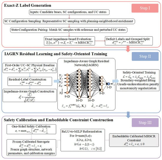
The original impedance-based MRSCR constraint formulated in Section 2 contains decision-dependent impedance matrix inversion and nonlinear coupling between UC states and SC configurations, and thus cannot be directly incorporated into the MILP. This section constructs an embeddable MRSCR constraint using the IAGRN. Exact impedance-based samples are first generated under sampled UC states and SC configurations. The IAGRN then learns the nonlinear residual relative to a first-order UC–SC physical baseline. One-sided calibration is applied to reduce the risk of false safe predictions, followed by mixed-integer linear reformulation for embedding the trained network into the planning model. The complete construction procedure is illustrated in Figure 2.

Figure 2. Flowchart of IAGRN-based embeddable MRSCR constraint construction.

3.1. Exact Label and Physical Residual Construction

To capture the combined effects of SC allocation and synchronous unit commitment on MRSCR, the training data are generated by pairing a planning-oriented set of SC configurations with hourly UC states. The configuration set combines zero SC, single-site, same-site multi-module, two-site interaction, planning neighborhood, and capacity stratified random samples. The hourly schedules obtained from the baseline UC serve as reference states, and bounded perturbations of the online equivalent unit counts are introduced to represent nearby commitment patterns considered in coordinated planning.

The dataset contains 39,451 observations covering 3858 distinct SC configurations and 192 representative operating hours. Each observation includes exact MRSCR labels for 26 renewable POIs. The configuration grouped split yields 20,782 training, 10,673 calibration, and 7996 test observations. UC variations are generated around the reference hourly commitment states. With a probability of 0.5, one to three sequential perturbations are attempted, each increasing or decreasing the online count of a randomly selected generating cluster by one unit. Perturbations are accepted only if the cluster unit count bounds and the aggregate generation capacity limits remain consistent with the reference total dispatch.

For each state–configuration pair, the short-circuit impedance matrix is reconstructed using Equations (34)–(36), and the exact simplified MRSCR is evaluated according to Equation (39) using the available renewable injections. Accordingly, the corresponding deficit label is defined by Equation (41).

$$d_{j,r,t}^{\mathrm{ex}}={\gamma }^{\min }-{\mathrm{MRSCR}}_{j,r,t}^{\mathrm{ex}}.$$

(41)

Here, j, r and t denote the observation, renewable POI, and hour, respectively. A positive value of $d_{j,r,t}^{\mathrm{ex}}$ indicates that the MRSCR requirement is violated. A first-order physical baseline is constructed around the reference UC state without newly installed SCs. The incremental effects of SC installation and synchronous unit commitment are obtained through one-module and one-unit finite differences, respectively:

$${\kappa }_{r,i,t}^{\mathrm{SC}}=d_{r,t}^{\mathrm{ex}}\left(u_t^0,e_i\right)-d_{r,t}^0,$$

(42)

$${\kappa }_{r,g,t}^g={\displaystyle \frac{d_{r,t}^{\mathrm{ex}}\left(u_t^0+{\delta }_{g,t}{e}_g,0\right)-d_{r,t}^0}{{\delta }_{g,t}}}.$$

(43)

where $d_{r,t}^0$ is the MRSCR deficit under the reference UC state without newly installed SCs; $u_t^0$ is the corresponding reference vector of online equivalent unit counts; e_i represents one SC module installed at candidate bus i; e_g represents a one-unit change in the online count of generation cluster g; and δ_g,t ∈ {−1,1} denotes the feasible perturbation direction. The first-order deficit is obtained by superposing the individual SC and UC increments:

$$d_{j,r,t}^{\mathrm{lin}}=d_{r,t}^0+{\displaystyle \sum _i{\kappa }_{r,i,t}^{\mathrm{SC}}}{n}_{j,i}^{\mathrm{SC}}+{\displaystyle \sum _g{\kappa }_{r,g,t}^g}\left(u_{j,g,t}-u_{g,t}^0\right).$$

(44)

Equation (44) does not explicitly represent the nonlinear interactions caused by multiple SC installations, simultaneous UC variations, and impedance matrix inversion. These effects are retained in the residual label by Equation (45):

$$r_{j,r,t}^{\mathrm{lab}}=d_{j,r,t}^{\mathrm{ex}}-d_{j,r,t}^{\mathrm{lin}}.$$

(45)

The residual in Equation (45) is used as the learning target of the IAGRN. The samples are assigned to the training, calibration, and test sets by complete SC configuration. All observations associated with the same configuration remain in the same subset to prevent configuration leakage.

3.2. IAGRN Residual Learning and Safety-Oriented Training

The IAGRN constructs an impedance coupling graph whose nodes include the SC candidate buses and renewable POIs. The reference impedance matrix Z⁰ is calculated once from the passive network and the fixed equivalents of existing synchronous support, excluding online generators and newly installed SCs. The normalized electrical coupling between nodes i and k is defined by Equation (46):

$$A_{\mathit{ik}}^Z={\displaystyle \frac{\left|Z_{\mathit{ik}}^0\right|}{\sqrt{\left|Z_{\mathit{ii}}^0\right|\left|Z_{\mathit{kk}}^0\right|}}}$$

(46)

where $Z_{\mathit{ik}}^0$ is the corresponding element of the reference impedance matrix Z⁰. The graph structure remains fixed, while the effects of UC states and newly installed SCs are represented by node features. For sample j at hour t, the feature vector of node i is expressed by Equation (47):

$$x_{i,j,t}={\left[x_{i,j,t}^1,x_{i,j,t}^2,\dots ,x_{i,j,t}^9\right]}^{\mathrm{T}}.$$

(47)

The nine features describe the installed SC module count, local online synchronous capacity, impedance coupled synchronous capacity, available renewable power, candidate bus indicator, POI indicator, nominal voltage level, reference self-impedance, and existing synchronous support. All node features are normalized using fixed scaling factors determined before training, and the same factors are retained during planning. The local and impedance coupled online synchronous capacities are calculated by Equations (48) and (49), respectively:

$$S_{i,j,t}^l={\displaystyle \sum _{g:b_g=i}{P}_g^{\max }}{u}_{g,j,t}.$$

(48)

$$S_{i,j,t}^c={\displaystyle \sum _{g\in \mathcal{G}}{A}_{i,b_g}^Z}{P}_g^{\max }{u}_{g,j,t}.$$

(49)

where b_g is the bus of generation cluster g, $P_g^{\max }$ is the maximum active power output of one equivalent unit, and u_g,j,t is the number of online equivalent units. The node features are propagated through two graph layers. Each layer combines the node itself with the electrically coupled neighboring nodes, as expressed in Equation (50).

$$H^{\left(l\right)}=\sigma \left(H^{\left(l-1\right)}{W}_s^{\left(l\right)}+A^Z{H}^{\left(l-1\right)}{W}_n^{\left(l\right)}+b^{\left(l\right)}\right),l=1,2,$$

(50)

where H⁽⁰⁾ = X, ${\mathbf{W}}_s^{\left(l\right)}$ and ${\mathbf{W}}_n^{\left(l\right)}$ are trainable weights, and σ(⋅) denotes the ReLU function. The input layer contains nine features for each graph node. The first graph layer maps the input into a 16-dimensional hidden representation, and the second graph layer retains the same dimension. The representations of the renewable POIs are then extracted and passed through an eight-neuron ReLU layer and a one-neuron linear output layer. The resulting 9–16–16–8–1 architecture outputs the nonlinear residual of the MRSCR deficit at each renewable POI. The predicted deficit is obtained by combining this residual with the first-order physical baseline:

$${\widehat{d}}_{r,j,t}=d_{r,j,t}^{\mathrm{lin}}+{\widehat{r}}_{r,j,t}$$

(51)

The IAGRN is trained using the composite objective defined in Equation (52), which considers prediction accuracy near the security boundary, unsafe underestimation, and the monotonic effect of SC installation:

$ℒ$ = $ℒ$_f + λ_u$ℒ$_u + λ_m$ℒ$_m.

(52)

$${\mathcal{L}}_f={\displaystyle \frac{1}{N}}{\displaystyle \sum _{r,j,t}\left(1+\beta e^{-\left|d_{r,j,t}^{\mathrm{ex}}\right|/\tau }\right)}\sqrt{{({\widehat{d}}_{r,j,t}-d_{r,j,t}^{\mathrm{ex}})}^2+{\eta }^2}$$

(53)

$${\mathcal{L}}_u={\displaystyle \frac{1}{N}}{\displaystyle \sum _{r,j,t}{[d_{r,j,t}^{\mathrm{ex}}-{\widehat{d}}_{r,j,t}]}_{+}^2}$$

(54)

$${\mathcal{L}}_m={\displaystyle \frac{1}{N_m}}{\displaystyle \sum _{r,j,t}{[d_{r,j,t}^{+}-{\widehat{d}}_{r,j,t}]}_{+}^2}$$

(55)

where N is the number of training label entries; N_m is the number of paired entries used for monotonicity regularization; λ_u and λ_m are the corresponding loss weights; β, τ, and η are training parameters; and [x]₊ = max(x,0). The term ${\widehat{d}}_{r,j,t}$ denotes the predicted deficit after adding one SC module. The three loss terms emphasize boundary region accuracy, penalize unsafe underestimation, and enforce a non-increasing MRSCR deficit with increasing SC capacity. The IAGRN is trained using Adam for 60 epochs with a batch size of 256 and a learning rate of 0.001. The loss parameters are set to β = 20, τ = 0.20, λ_u = 1, and λ_m = 1.

3.3. Safety Calibration and Embeddable Constraint Construction

The calibration set is excluded from parameter training and is used only to determine fixed one-sided safety margins. The POI-specific unsafe classification margin, shared boundary margin, and final margin are calculated as follows:

$${ϵ}_r^u=\max (0,\max (d_{r,j,t}^{\mathrm{ex}}-{\widehat{d}}_{r,j,t})), \left(j,t\right)\in {\mathcal{D}}^{\mathrm{cal}}, d_{r,j,t}^{\mathrm{ex}}>0$$

(56)

$${ϵ}^b=\max (0,\max (d_{q,j,t}^{\mathrm{ex}}-{\widehat{d}}_{q,j,t})),q\in R, d_{q,j,t}^{\mathrm{ex}}\ge -\Delta$$

(57)

$${ϵ}_r=\max \left({ϵ}_r^u,{ϵ}^b\right)+\xi$$

(58)

where $𝒟$^cal is the calibration set; q indexes the renewable POIs considered in the shared margin; Δ defines the boundary-relevant region; and ξ is a small positive tolerance. The POI-specific margin prevents truly unsafe calibration samples from being classified as safe, while the shared margin limits deficit underestimation near the security boundary across all renewable POIs. The calibrated deficit is expressed as follows:

$${\widehat{d}}_{r,j,t}^{\mathrm{cal}}={\widehat{d}}_{r,j,t}+{\epsilon }_r$$

(59)

The graph structure, feature normalization parameters, trained weights, and calibration margins are fixed before planning. For an unstable ReLU h = max(0,a) with L < 0 < U, its exact mixed-integer linear representation is

h ≥ a,   h ≥ 0

(60)

h ≤ a − L(1 − z),

(61)

h ≤ Uz,z ∈ {0,1}.

(62)

ReLU units satisfying L > 0 or U < 0 are directly reduced to h = a or h = 0, respectively. The pre-activation bounds L and U are computed layer by layer through interval propagation from the admissible bounds of the SC module and online unit variables. The calibrated IAGRN constraint embedded in the coordinated planning model is

$${\widehat{d}}_{r,k,t}^{\mathrm{cal}}\le 0,r\in \mathcal{R},k\in \mathcal{D},t\in \mathcal{T}.$$

(63)

The resulting formulation provides a mixed-integer linear representation of the calibrated UC-dependent MRSCR surrogate.

4. Case Studies

4.1. System and Case Settings

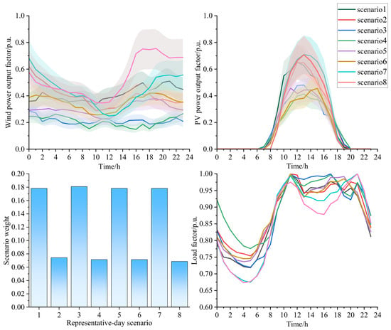
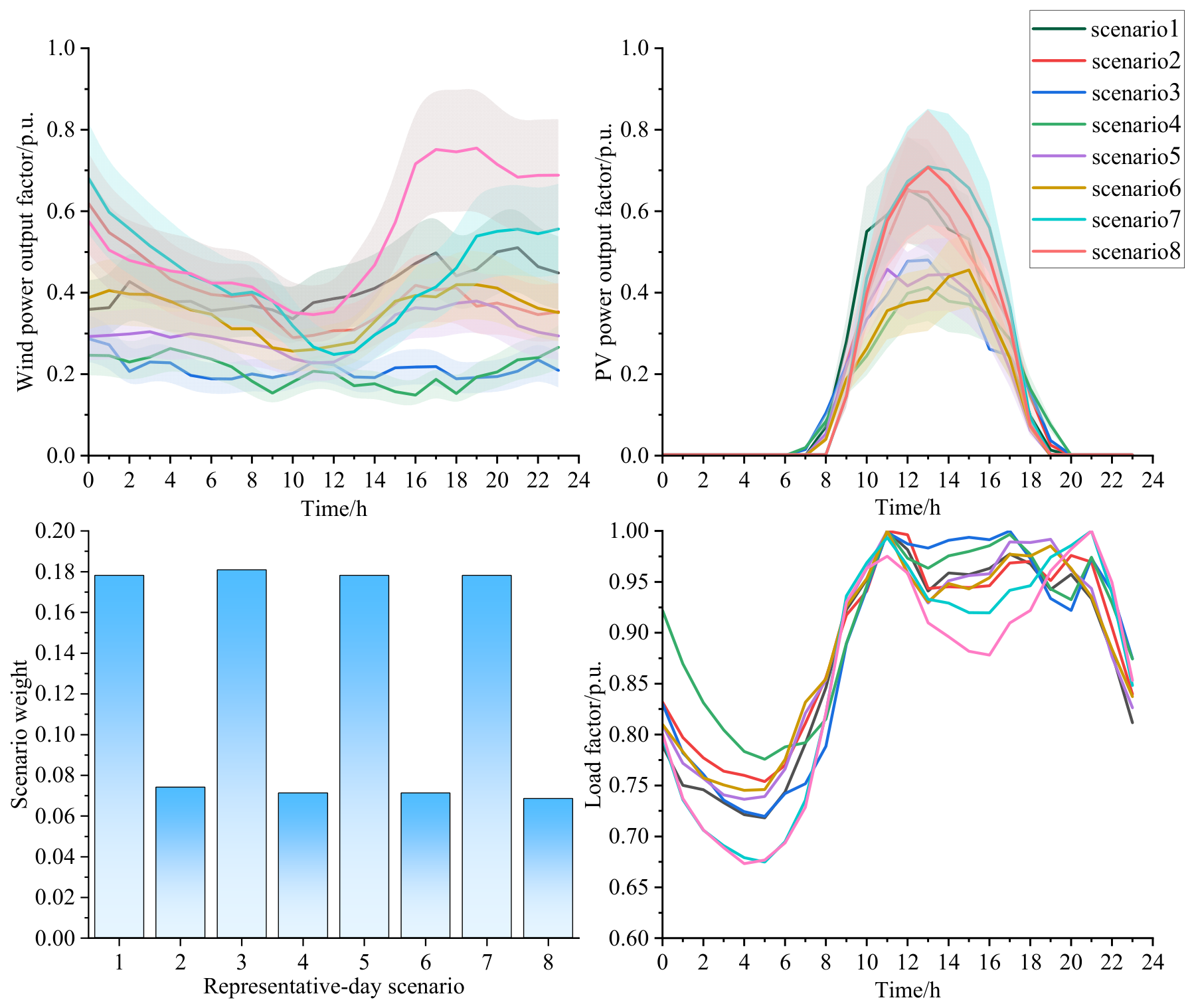
The case study is conducted on a provincial-scale aggregated system comprising 106 buses, 283 branches, 125 synchronous unit clusters, and 26 renewable POIs. For the planning year case, the load, wind capacity, PV capacity, and synchronous generation capacity are scaled to 1.30, 1.80, 2.00, and 1.05 times their respective baseline levels. All optimization problems are solved using Gurobi 12.0.1 under MATLAB R2023b on a PC equipped with an Intel Core i7-14700 processor and 16 GB of RAM, with the relative optimality gap tolerance (MIPGap) set to 0.001. The daily load factor, wind power output factor, and PV power output factor profiles are used as input features for K-means clustering. With the number of clusters set to eight, the cluster centers define the 24 h representative day profiles, and the weight of each scenario is determined by the proportion of days assigned to the corresponding cluster. The representative profiles are combined with the planning year load and installed capacities to construct 192 hourly operating states. The resulting profiles and scenario weights are shown in Figure 3.

Figure 3. Representative day load, wind power, and PV power profiles and scenario weights.

The principal system and planning parameters are summarized in Table 1. SC and SVG capacities are discretized into 300 Mvar and 100 Mvar modules, respectively, with per-bus limits of three SC modules and six SVG modules. The MRSCR security threshold is set to 2.5 [5]. Following the screening procedure described in Section 2.2, the initial 50 bus candidate pool is expanded to 56 buses through two bounded refreshes and subsequently fixed for IAGRN dataset construction and coordinated planning. The proposed model is implemented in MATLAB R2023b using YALMIP and solved with Gurobi 12.0.1.

Table 1. Main parameters used in case study.

Symbol	Parameter	Value	Unit
SB	System power base	100	MVA
$\left[q_{\min }^{\mathrm{SC}},q_{\max }^{\mathrm{SC}}\right]$	Reactive power range of each SC module	[−150, 300]	Mvar
$\left[q_{\min }^{\mathrm{SVG}},q_{\max }^{\mathrm{SVG}}\right]$	Reactive power range of each SVG module	[−100, 100]	Mvar
Km	SC/SVG investment cost per module	1.65/0.50	108 RMB
Lm	SC/SVG service life	30/20	year
μm	SC/SVG annual fixed O&M ratio	5.0/2.2	%
ξSC/ξSVG	SC/SVG active loss ratio	1.5/1.0	%
$x_{\mathrm{SC}}^{\prime }{S}^{\mathrm{SC}}/x_g^{\prime }{S}_g$	SC/synchronous unit transient reactance factor	0.10/0.15	p.u.
$c_g^p$	Coal/gas/hydro energy production cost	300/500/20	RMB/MWh
$c_g^y/P_g^{\max }$	Startup cost rate of coal/gas/hydro units	1500/300/20	RMB/MW
ρu/ρd	Upward/downward reserve requirement	5/5	% of load
cw/cs	Wind/PV curtailment penalty	430/550	RMB/MWh
ch	Hydropower spillage penalty	350	RMB/MWh

4.2. Planning Results

Four planning schemes are compared to evaluate the roles of SCs and SVGs in satisfying the MRSCR requirement:

S1 neglects the MRSCR constraint and allows for coordinated SC–SVG planning;

S2 considers the MRSCR constraint but permits only SC installation;

S3 considers the MRSCR constraint but permits only SVG installation;

S4 represents the proposed coordinated SC–SVG planning scheme. The results are summarized in Table 2.

Table 2. Comparison of planning results under different schemes.

Scheme	SC Allocation: Bus (Mvar)	SVG Allocation: Bus (Mvar)	Annualized Investment (108 RMB)	Total Annual Cost (108 RMB)	Minimum Exact MRSCR	Optimization Runtime (s)	Final MIP Gap (%)	Result
S1	70 (300)	67 (600), 68 (400), 70 (600)	1.147	1190.634	1.823	619.01	0.0557	21 violations
S2	2 (600), 25 (600), 27 (300), 28 (600), 29 (600), 31 (900), 32 (600), 38 (600), 67 (900), 70 (900), 85 (900);	—	5.387	1202.779	2.555	1802.98	0.0875	Feasible
S3	—	—	—	—	—	—	—	Infeasible
S4	2 (600), 25 (300), 26 (600), 27 (300), 31 (600), 32 (300), 33 (300), 35 (300);	67 (600), 68 (600), 70 (600)	3.418	1197.748	2.711	2213.86	0.0694	Feasible

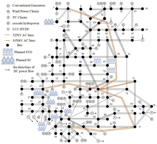
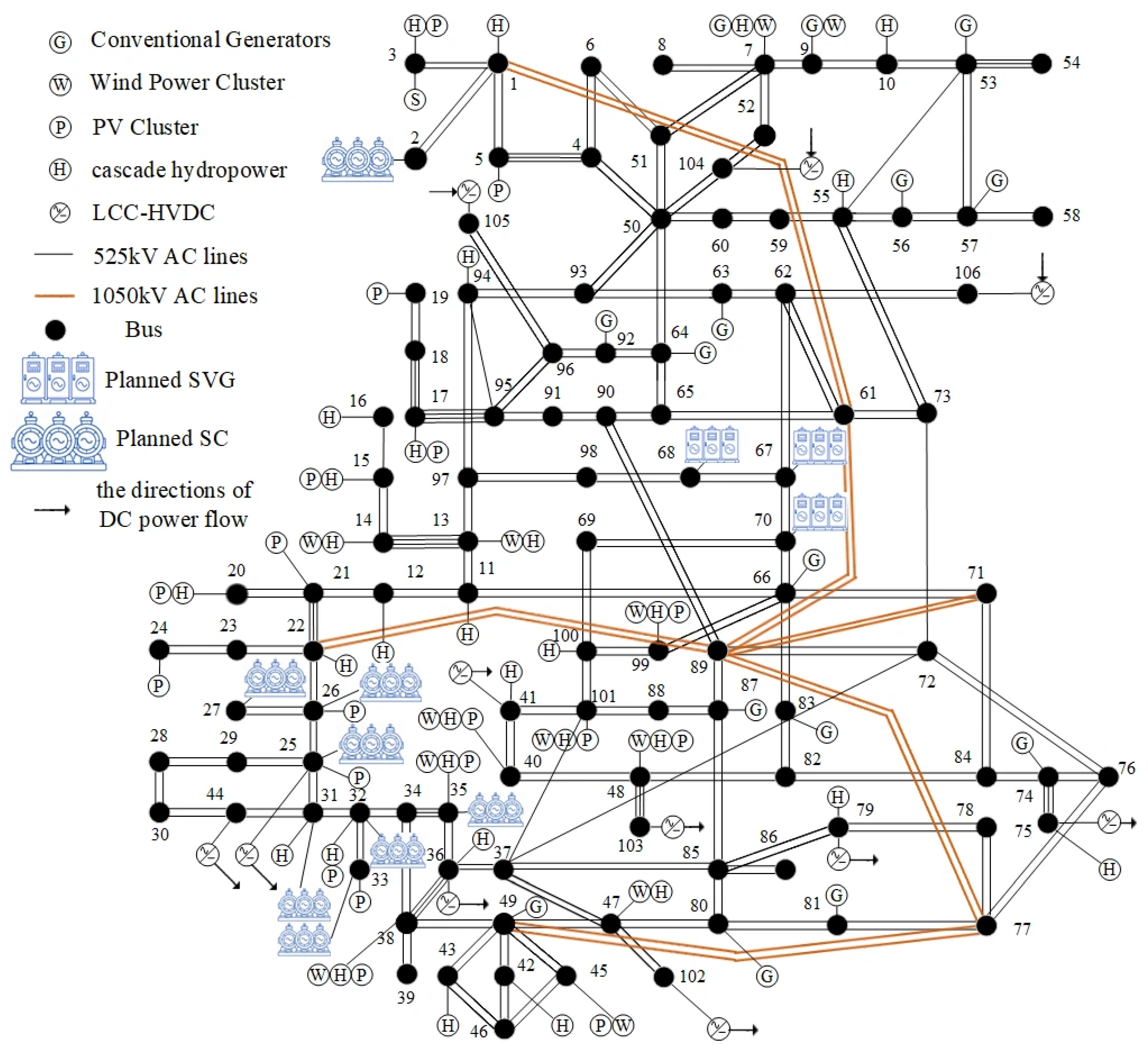
Table 2 shows that the least cost planning scheme is not necessarily secure. When the MRSCR constraint is omitted, S1 yields a minimum exact simplified MRSCR of 1.823, with 21 hourly operating states in which at least one renewable POI falls below the prescribed threshold. Thus, satisfying the conventional operational constraints alone does not ensure adequate grid strength. S2 eliminates all MRSCR violations by installing 7500 Mvar of SC capacity but incurs the highest annualized investment among the MRSCR feasible schemes. S3 remains infeasible because SVGs do not directly strengthen MRSCR, while the available synchronous support under feasible UC schedules is insufficient to satisfy all MRSCR constraints. By coordinating the two devices, S4 uses SCs to strengthen the system and SVGs to provide lower cost reactive power support. It reduces the required SC capacity to 3300 Mvar while maintaining a minimum exact simplified MRSCR of 2.711 across all 192 operating states. Compared with S2, its annualized investment is reduced by 36.6%. Schemes S1, S2, and S4 all converge within the prescribed MIP gap tolerance of 0.1%, while S4 requires a longer computational time due to the increased number of constraints. The resulting SC and SVG allocation under S4 is shown in Figure 4.

Figure 4. Final SC and SVG allocation under Scheme S4.

As shown in Figure 4, SCs are mainly located in the Bus 25–35 area, where large renewable power injections coincide with relatively weak pre-planning MRSCR values. Their installation increases the local short-circuit support and improves the grid strength of the associated renewable POIs. In contrast, Buses 67, 68, and 70 are among the main load buses and have no local synchronous generation; SVGs are therefore installed at these buses to provide controllable reactive power close to the load center. The planning result thus assigns SCs primarily to grid strength reinforcement and SVGs to local voltage and reactive power support.

4.3. Operating Results

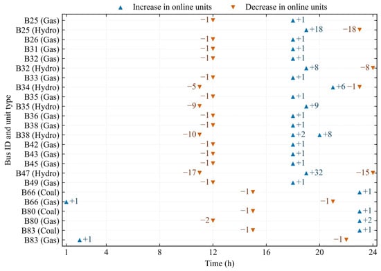
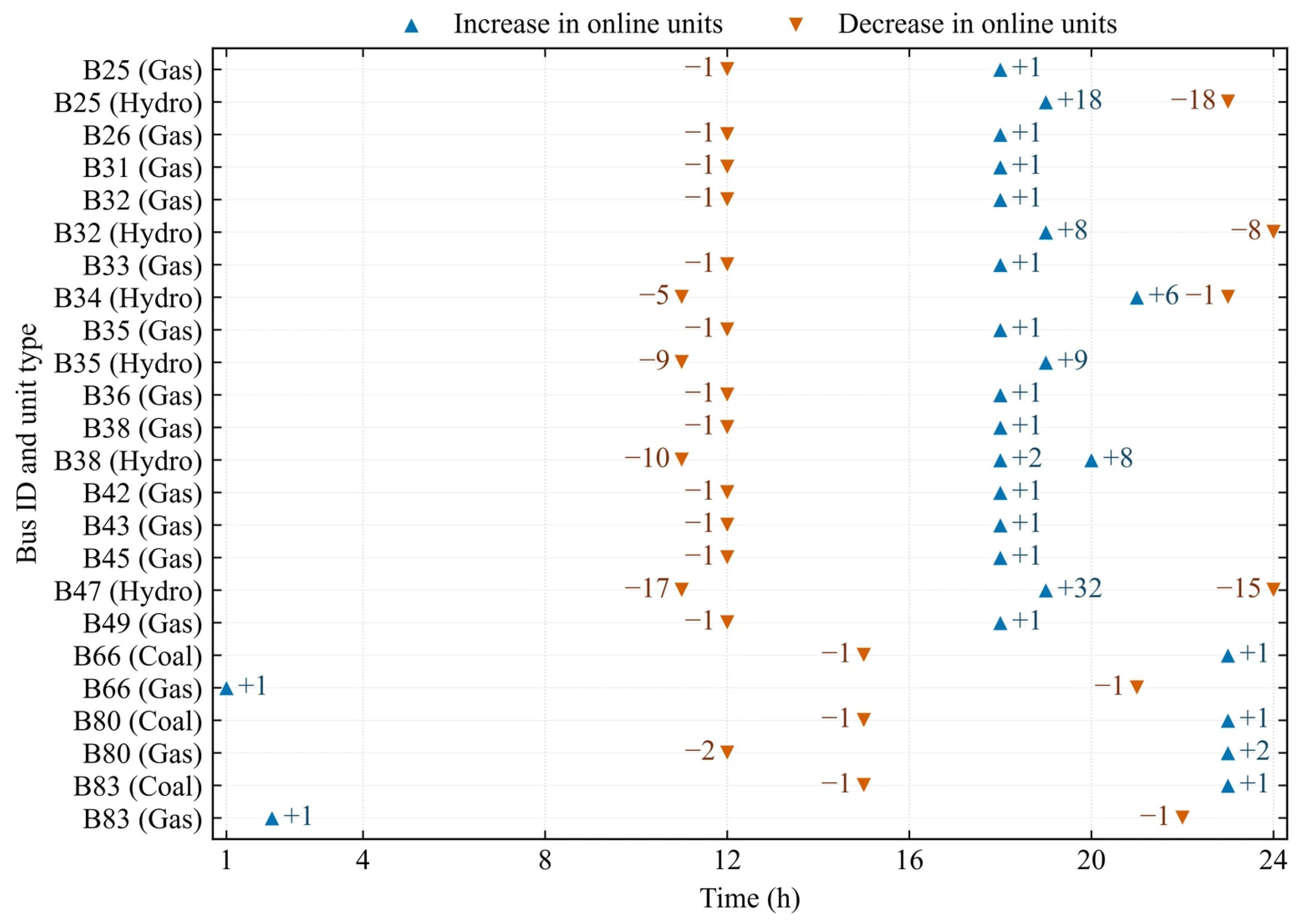
To examine the relationship among unit commitment, power dispatch, and system strength, the hourly operating results for a representative day are analyzed. Figure 5 presents the hourly commitment adjustments on the selected representative day. Online unit counts vary in 24 synchronous unit clusters, with reductions concentrated around hours 11–12 and increases mainly during hours 18–20. Gas clusters generally exhibit small adjustments, whereas hydro clusters account for larger changes in online unit counts. This temporal pattern is consistent with the midday increase and evening decline in PV output shown in Figure 3.

Figure 5. Hourly changes in the number of online equivalent units on the representative day.

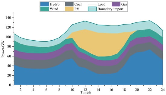
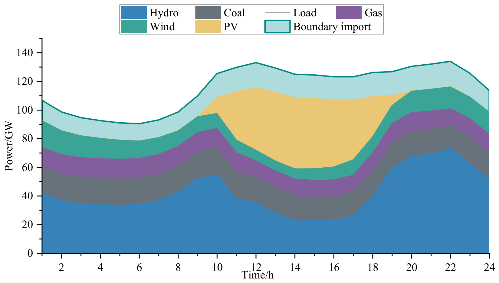
The active power supply composition in Figure 6 further explains these commitment adjustments. During the midday period, the increase in PV generation is accompanied by a reduction in hydro output, while coal and gas generation remain comparatively stable. As PV output declines in the evening, hydro output increases to meet the remaining demand. The consistency between the generation composition and commitment changes indicates that hydropower provides much of the intraday balancing in this case. Boundary imports are included in the supply composition.

Figure 6. Hourly active power supply composition on the representative day.

These results show that the changing renewable output is accommodated through both dispatch and commitment adjustments. Changes in online unit counts modify the synchronous source admittance and hence the impedance matrix used to calculate MRSCR. The planned equipment allocation must therefore satisfy the system strength requirement across the hourly UC states. The corresponding MRSCR security performance is assessed in the following section.

4.4. MRSCR Security Assessment

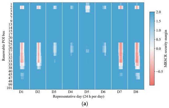
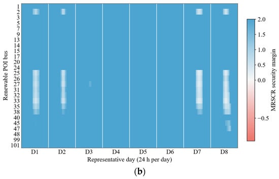
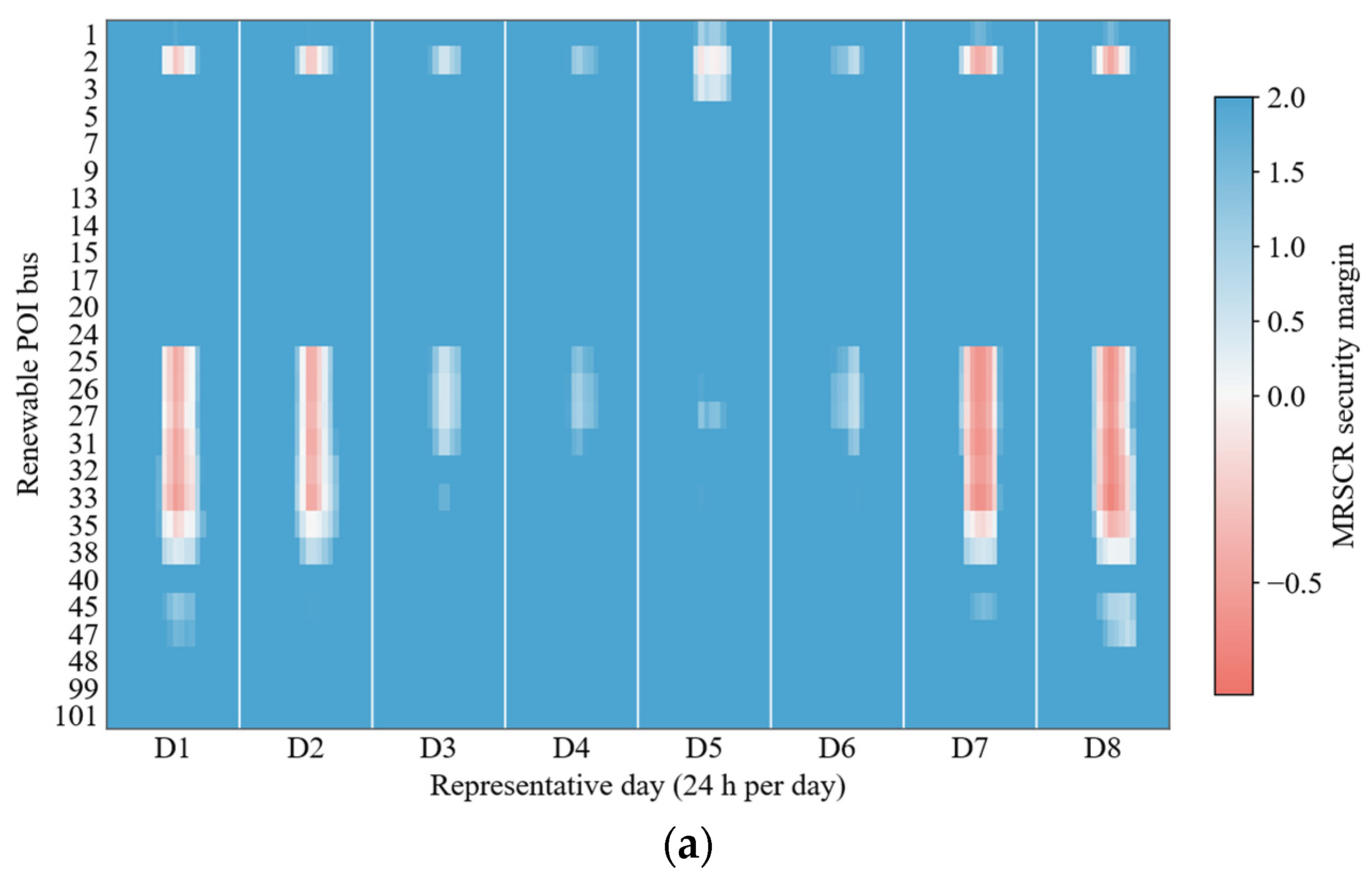
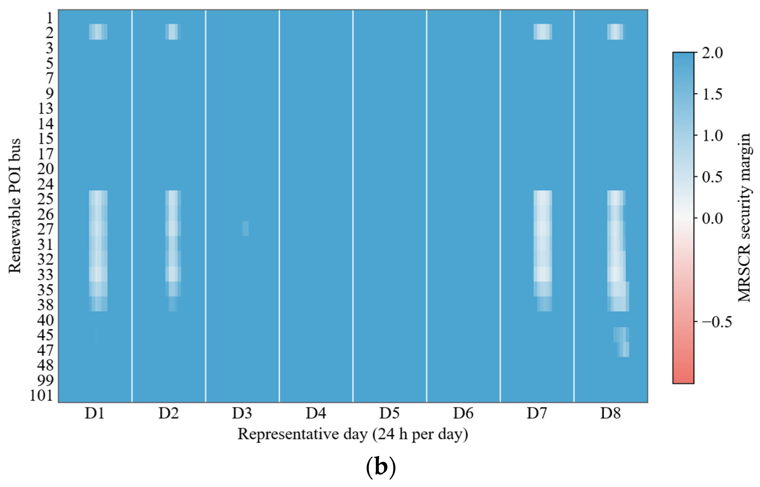
The system strength adequacy of the planning solution is evaluated by reconstructing the hourly short-circuit impedance matrices using the optimized SC allocation and UC states. The exact simplified MRSCR is then calculated at each renewable POI over the 192 representative operating hours. Figure 7 compares the security margins before planning and after implementing Scheme 4, where the margin is defined as the exact simplified MRSCR minus the threshold of 2.5. Before planning, negative margins are concentrated at a limited number of renewable POIs during specific operating periods. This distribution indicates that system strength deficiencies depend on both the connection location and the operating state. Following coordinated planning, the negative margin regions disappear, and the minimum exact simplified MRSCR reaches 2.711. All 4992 POI–hour operating points satisfy the prescribed threshold, confirming that the planning solution meets the MRSCR requirement across the evaluated representative days.

Figure 7. MRSCR security margins before and after coordinated SC–SVG planning: (a) before planning; (b) after S4 planning.

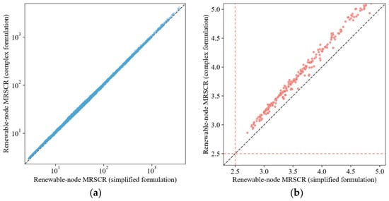
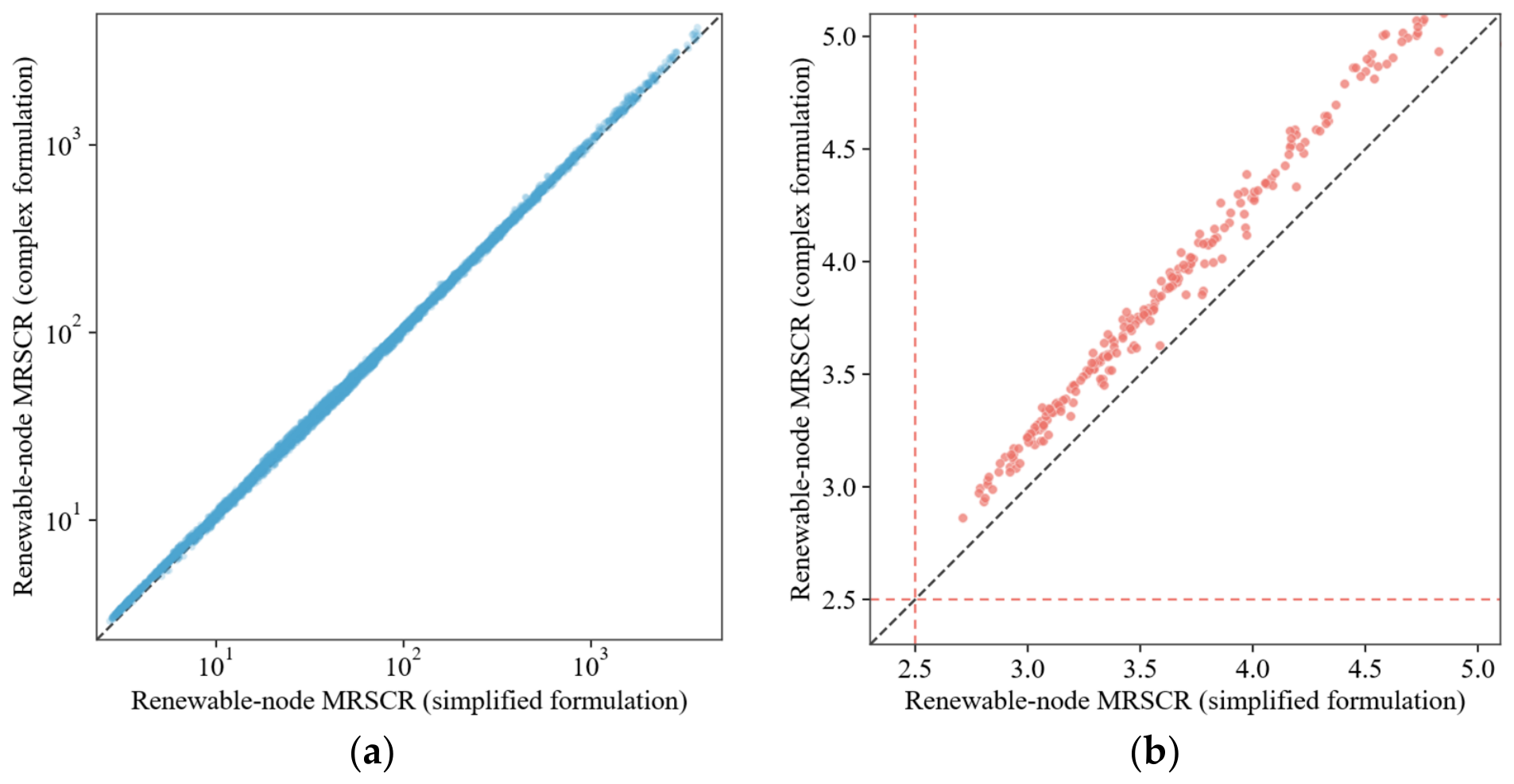
The consistency between the simplified and full complex formulations in Equations (39) and (37), respectively, is further examined under the same planned configuration and hourly UC states. Both formulations are evaluated using available renewable power to ensure a consistent injection basis. Figure 8 presents the comparison for all renewable POI–hour operating points, together with an enlarged view near the security threshold. The diagonal line denotes equality between the two formulations.

Figure 8. Comparison of MRSCR values calculated using the simplified and full complex formulations: (a) all renewable POI–hour operating points; (b) operating points near the security threshold. Blue points show the full set of operating points, while red points highlight the near-threshold region.Gray dashed diagonal lines indicate equality between the two formulations, and red dashed horizontal and vertical lines mark the MRSCR security threshold of 2.5.

The two formulations follow a similar trend over the full range of MRSCR values, although the enlarged view reveals differences near the security threshold. In the displayed near-threshold region, the full complex formulation generally yields higher values than the simplified formulation. The simplified calculation therefore provides a conservative assessment for these operating points. These results support the use of the simplified formulation as the planning constraint in this case, while the full complex formulation is used for exact post-planning verification.

4.5. IAGRN Prediction Accuracy and Safety Calibration

Randomly sampled SC configurations are split into training, calibration, and test sets at a target ratio of 13:4:3, while structural and anchor configurations are assigned to training and additional operating-hour samples are included in calibration and testing, with no configuration overlap among the sets. The IAGRN is compared with an MLP and an impedance-based GNN on the same test set, focusing on prediction accuracy near the MRSCR security threshold and false safe classifications. The results before calibration are summarized in Table 3.

Table 3. Performance comparison of different prediction models.

Method	Near-Boundary MAE	Node-Level False Safe (Count; Rate)	Observation-Level False Safe (Count; Rate)
MLP	0.1186	947; 6.08%	217; 7.00%
Impedance-based GNN	0.0739	571; 3.66%	126; 4.06%
IAGRN	0.0101	240; 1.54%	36; 1.16%

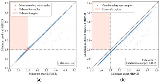
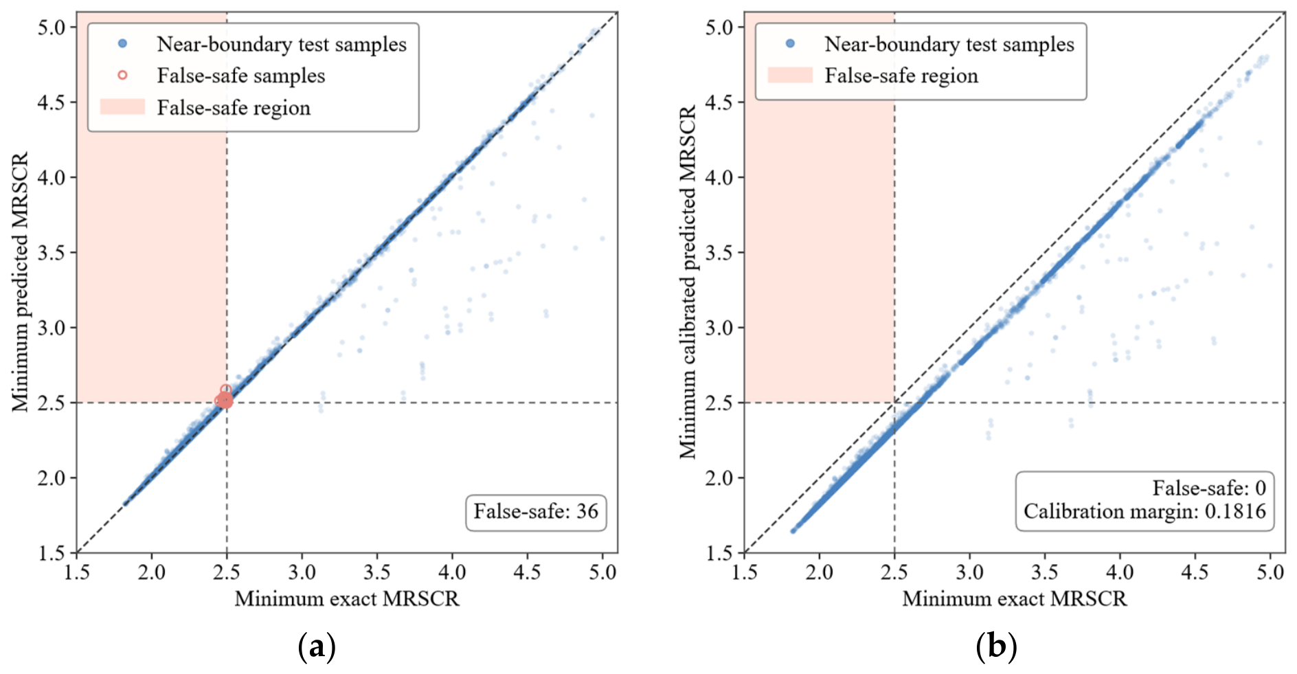
Near-boundary MAE is evaluated over the exact MRSCR interval of 2.3–2.7. A false safe node pair occurs when a renewable POI is predicted to satisfy the MRSCR threshold but violates it under exact evaluation. The node-level false safe rate is calculated as the number of false safe node pairs divided by the number of node pairs that are exactly unsafe. A false safe observation occurs when all POIs are predicted to be safe while at least one POI is exactly unsafe. The observation-level false safe rate is calculated as the number of false safe observations divided by the number of test observations containing at least one exactly unsafe POI. The comparison shows that the IAGRN achieves lower near-boundary MAE and fewer false safe classifications at both the node and observation levels. By learning nonlinear residuals from the first-order physical baseline over the impedance coupling graph, the model captures the combined effects of SC allocation and UC states while retaining the underlying physical trend. These characteristics make the IAGRN more suitable for security-constrained planning than the benchmark models. The remaining false safe predictions are addressed through one-sided calibration, with the calibration margins determined exclusively from the calibration set. Figure 9 compares the minimum exact and predicted MRSCR values for test observations whose minimum exact MRSCR does not exceed 5. Before calibration, some observations fall within the shaded false safe region, where the predicted minimum MRSCR satisfies the threshold while the exact value remains below it.

Figure 9. Effect of one-sided calibration on IAGRN safety predictions: (a) uncalibrated predictions; (b) calibrated predictions. The diagonal dashed lines represent y = x, indicating perfect agreement between the predicted and exact MRSCR values. The horizontal and vertical dashed lines indicate the MRSCR security threshold of 2.5.

For the present dataset, the shared boundary margin is larger than the POI-specific unsafe classification margin at every renewable POI. With the numerical tolerance included, the resulting fixed calibration margin is 0.181581. Applying this margin eliminates all 36 false safe observations in the held-out test set. The calibration margin is determined from an independent calibration set covering different SC configurations and UC states, and remains fixed during planning. Changes in SC installation locations and capacities are reflected in the IAGRN predictions, while the calibration margin provides a common safety correction over the considered configuration range.

To further assess generalization, the trained IAGRN is evaluated on four additional operating days beyond the eight representative days, with the calibration margin kept unchanged. As shown in Table 4, the calibration substantially reduces false safe observations under unseen load, renewable generation, and UC conditions.

Table 4. Generalization performance under unseen operating conditions.

Operating Condition	Observations	Near-Boundary MAE	False Safe Before Calibration	False Safe After Calibration
Peak load	1200	0.0138	9	0
High renewable penetration	1200	0.0175	14	1
Low synchronous generation commitment	1200	0.0226	21	2
Large net-load fluctuations	1200	0.0209	17	1

4.6. Transient Simulation Validation

To further evaluate the transient voltage performance, the planning solutions obtained under S1 and S4 are implemented in PSD-BPA and denoted as Schemes 1 and 4, respectively. The dynamic models and main control parameters adopted in the PSD-BPA simulations are summarized in Table 5.

Table 5. Dynamic models and control parameters used in PSD-BPA simulations.

Component	Dynamic Model	Control Configuration	Main Parameters
Synchronous generator	MG/MF	FV/F+ excitation, GH/GN governors, PSS where applicable	Representative hydro unit: H = 4.44 s; D = 2.0; T′d0 = 7.8 s; T′q0 = 1.5 s; KA = 30.0; TA = 0.04 s; VRMAX/VRMIN = 5.0/−5.0 p.u.
SC	Synchronous machine	Voltage-regulating excitation; no governor	H = 2.0 s; excitation voltage limits: 0–5.0 p.u.
SVG	VG/VG+	Constant-voltage control; low-voltage blocking and reconnection	Measurement time constant: 0.01 s; response delay: 0.02 s; current limits: ±1.0 p.u.; blocking/reconnection thresholds: 0.20/0.90 p.u.; reconnection delay: 0.02 s
Wind power	MM with ES/EV	DFIG control; reactive current priority; LVRT	Total, active, and reactive current limits: 1.2 p.u.; LVRT thresholds: 0.84/0.913 p.u.; detection delay: 0.5 cycles
PV power	MS with ES/EV	Converter current limiting; LVRT and HVRT	Current limits: 1.2 p.u.; LVRT thresholds: 0.84/0.913 p.u.; HVRT thresholds: 1.10/1.05 p.u.; detection delay: 0.5 cycles
Load	Static load and MJ	Static and induction motor loads	Induction motor proportion: 30% in specified areas

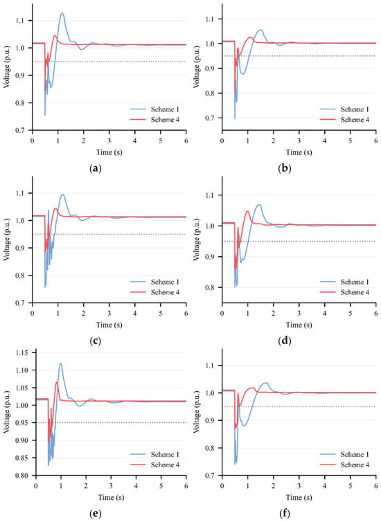
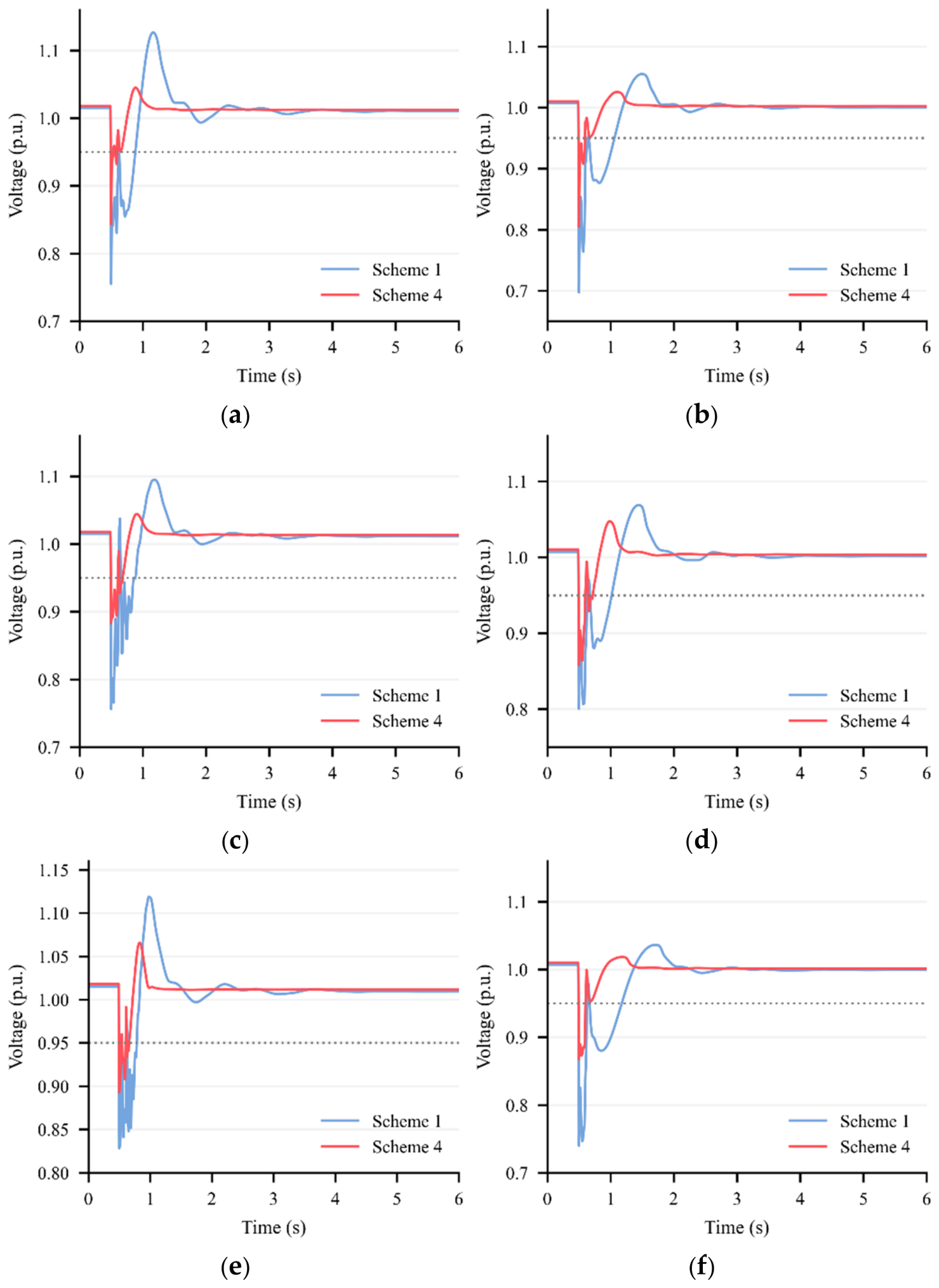
Three fault scenarios, F1, F2, and F3, are considered on Lines 50–93, 13–97, and 47–49, respectively. The system initially operates under steady-state conditions. In each scenario, a three-phase short-circuit fault is applied at the selected terminal of the line at 0.5 s. Three fault durations of 0.10, 0.15, and 0.20 s are considered, with the faulted line disconnected at 0.60, 0.65, and 0.70 s, respectively. The simulation time step is set to 0.5 cycles (0.01 s for a 50 Hz system). Figure 10 compares the transient voltage responses at Buses 35 and 67 under Schemes 1 and 4 for the 0.10 s fault duration. Table 6 summarizes the minimum voltages and post-fault recovery times for each scenario. The recovery time is defined as the elapsed time from fault clearance until the voltage reaches 0.95 p.u. and remains at or above this threshold for the remainder of the simulation.

Figure 10. Transient voltage responses under Schemes 1 and 4 for three fault scenarios: F1 (a,b); F2 (c,d); F3 (e,f). The left and right panels show Buses 35 and 67, respectively.The horizontal dotted lines indicate the voltage recovery threshold of 0.95 p.u.

Table 6. Minimum voltages and post-fault recovery times under Schemes 1 and 4.

Fault Scenario/Monitoring Point	Fault Duration (s)	Minimum Voltage S1 (p.u.)	Minimum Voltage S4 (p.u.)	Recovery Time S1 (s)	Recovery Time S4 (s)
F1/Bus 35	0.10	0.7552	0.8416	0.29	0.05
	0.15	0.7552	0.8416	1.75	0.20
	0.20	0.7110	0.8124	3.23	0.28
F1/Bus 67	0.10	0.6976	0.8073	0.47	0
	0.15	0.6976	0.8073	1.54	0.13
	0.20	0.6881	0.8032	1.80	0.16
F2/Bus 35	0.10	0.7561	0.8828	0.29	0.09
	0.15	0.7298	0.8386	1.51	0.18
	0.20	0.7298	0.8386	1.78	0.20
F2/Bus 67	0.10	0.8003	0.8619	0.42	0.13
	0.15	0.7638	0.8566	1.55	0.17
	0.20	0.7638	0.8566	1.83	0.18
F3/Bus 35	0.10	0.8322	0.8937	0.19	0.06
	0.15	0.7884	0.8524	1.64	0.14
	0.20	0.7412	0.8052	1.84	0.17
F3/Bus 67	0.10	0.7379	0.8723	0.58	0.01
	0.15	0.7202	0.8346	1.59	0.16
	0.20	0.6716	0.7846	1.86	0.18

As shown in Figure 10 and Table 6, Scheme 4 consistently achieves higher voltage nadirs and shorter post-fault recovery times than Scheme 1 at both monitored buses under all three fault scenarios. Specifically, the minimum voltages increase by 0.0615–0.1344 p.u., while the recovery times are reduced by 0.13–2.95 s across the three fault durations (0.10, 0.15, and 0.20 s). Although longer fault durations generally result in lower voltage nadirs and longer recovery times, Scheme 4 maintains superior voltage recovery performance under all tested conditions. Moreover, Scheme 4 exhibits reduced voltage oscillations following fault clearance, as illustrated in Figure 10. These results indicate that coordinated SC–SVG planning effectively improves transient voltage support and post-fault voltage recovery under different fault locations and durations.

5. Conclusions

This paper proposes an SC–SVG coordinated planning method considering UC-dependent MRSCR constraints with large-scale renewable integration. The model jointly determines the siting and sizing of SCs and SVGs together with the hourly operation of synchronous generating units, thereby accounting for changes in the short-circuit impedance matrix caused by equipment allocation and UC states. To make the nonlinear, state-dependent MRSCR requirement tractable, a first-order UC–SC physical baseline is combined with an impedance-aware graph residual network to represent the remaining nonlinear effects. One-sided safety calibration reduces false safe predictions near the security threshold, while the mixed-integer linear reformulation enables the calibrated IAGRN to be embedded directly in the planning model. Case studies on a provincial aggregated system show that the proposed method satisfies the MRSCR requirement across all evaluated representative operating states while reducing the investment required by the SC only scheme. Exact impedance-based post-validation verifies MRSCR satisfaction, and transient simulations show improved voltage recovery under the tested fault scenarios.

Future work will explicitly model the dynamic reactive power response limits and device-specific time constants of renewable power plants, SCs, and SVGs. Voltage security boundaries extracted from time-domain simulations will be approximated as tractable planning constraints to coordinate the siting and sizing of fast and slow reactive power support devices.

References

- International Renewable Energy Agency (IRENA). Renewable Capacity Statistics 2026; IRENA: Abu Dhabi, United Arab Emirates, 2026; Available online: https://www.irena.org/Publications/2026/Mar/Renewable-capacity-statistics-2026 (accessed on 8 September 2026).
- Hatziargyriou, N.; Milanovic, J.; Rahmann, C.; Ajjarapu, V.; Canizares, C.; Erlich, I.; Hill, D.; Hiskens, I.; Kamwa, I.; Pal, B.; et al. Definition and classification of power system stability—Revisited and extended. IEEE Trans. Power Syst. 2021, 36, 3271–3281. [Google Scholar] [CrossRef] [Scilit]
- Soleimani, H.; Habibi, D.; Ghahramani, M.; Aziz, A. Strengthening power systems for net zero: A review of the role of synchronous condensers and emerging challenges. Energies 2024, 17, 3291. [Google Scholar] [CrossRef] [Scilit]
- Lin, Y.; Wang, B.; Guo, Q.; Zhao, H.; Sun, H. Short-circuit ratio and short-term voltage security constrained unit commitment in high wind power-penetrated power systems. IEEE Trans. Power Syst. 2024, 39, 5631–5644. [Google Scholar] [CrossRef] [Scilit]
- Sun, H.; Xu, S.; Xu, T.; Guo, Q.; He, J.; Zhao, B.; Yu, L.; Zhang, Y.; Li, W.; Zhou, Y.; et al. Definition and index of short circuit ratio for multiple renewable energy stations. Proc. CSEE 2021, 41, 497–505. [Google Scholar] [CrossRef]
- Yuan, H.; Xin, H.; Wu, D.; Wang, W.; Zhou, Y. Small-signal stability assessment of multi-converter-based renewable systems with STATCOMs based on generalized short-circuit ratio. IEEE Trans. Energy Convers. 2022, 37, 2889–2902. [Google Scholar] [CrossRef] [Scilit]
- Zhu, Y.; Green, T.C.; Zhou, X.; Li, Y.; Kong, D.; Gu, Y. Impedance margin ratio: A new metric for small-signal system strength. IEEE Trans. Power Syst. 2024, 39, 7291–7303. [Google Scholar] [CrossRef] [Scilit]
- Hadavi, S.; Mansour, M.Z.; Bahrani, B. Optimal allocation and sizing of synchronous condensers in weak grids with increased penetration of wind and solar farms. IEEE J. Emerg. Sel. Top. Circuits Syst. 2021, 11, 199–209. [Google Scholar] [CrossRef] [Scilit]
- Hadavi, S.; Saunderson, J.; Mehrizi-Sani, A.; Bahrani, B. A planning method for synchronous condensers in weak grids using semi-definite optimization. IEEE Trans. Power Syst. 2023, 38, 1632–1641. [Google Scholar] [CrossRef] [Scilit]
- Wang, J.; Zhang, J.; Hou, Q.; Zhang, N. Synchronous condenser placement for multiple HVDC power systems considering short-circuit ratio requirements. IEEE Trans. Power Syst. 2025, 40, 765–779. [Google Scholar] [CrossRef] [Scilit]
- Fouladi, E.; Mehrizi-Sani, A.; Bahrani, B. An MILP model for optimal placement and sizing of synchronous condensers in a weak grid. IEEE Trans. Ind. Appl. 2026, 62, 3023–3033. [Google Scholar] [CrossRef] [Scilit]
- Lee, J.; Jo, H.; Kim, S. Optimal determination of synchronous condenser placement and voltage setting for enhancing power system stability. Energies 2025, 18, 6474. [Google Scholar] [CrossRef] [Scilit]
- Liang, H.; Zhang, Y.; Liu, S.; Wu, J.; Fan, J.; Zhang, Y.; Yu, J.; Zhang, T.; Zhu, Z. Modeling and simulation on the hybrid solution of static var generator and synchronous condenser for unlocking power output limitation of wind farms integrated into weak grid. Energies 2025, 18, 471. [Google Scholar] [CrossRef] [Scilit]
- Chu, Z.; Teng, F. Coordinated planning for stability enhancement in high IBR-penetrated systems. IEEE Trans. Sustain. Energy 2025, 16, 700–715. [Google Scholar] [CrossRef] [Scilit]
- Gu, H.; Yan, R.; Saha, T.K.; Muljadi, E. System strength and inertia constrained optimal generator dispatch under high renewable penetration. IEEE Trans. Sustain. Energy 2020, 11, 2392–2406. [Google Scholar] [CrossRef] [Scilit]
- Chu, Z.; Teng, F. Short circuit current constrained UC in high IBG-penetrated power systems. IEEE Trans. Power Syst. 2021, 36, 3776–3785. [Google Scholar] [CrossRef] [Scilit]
- Zhang, X.; Liu, Y.; Zhao, J.; Liu, J.; Korkali, M.; Chen, X. Short-circuit current constrained unit commitment and transmission switching model for improving renewable integration: An MILP formulation. IET Gener. Transm. Distrib. 2022, 16, 1743–1755. [Google Scholar] [CrossRef] [Scilit]
- Kim, Y.K.; Lee, S.H.; Lee, G.S. Strength-constrained unit commitment in IBR-dominant power systems. iEnergy 2025, 4, 121–131. [Google Scholar] [CrossRef] [Scilit]
- Zhang, N.; Jia, H.; Hou, Q.; Zhang, Z.; Xia, T.; Cai, X.; Wang, J. Data-driven security and stability rule in high renewable penetrated power system operation. Proc. IEEE 2023, 111, 788–805. [Google Scholar] [CrossRef] [Scilit]
- Hou, Q.; Zhang, N.; Kirschen, D.S.; Du, E.; Cheng, Y.; Kang, C. Sparse oblique decision tree for power system security rules extraction and embedding. IEEE Trans. Power Syst. 2021, 36, 1605–1615. [Google Scholar] [CrossRef] [Scilit]
- Jia, H.; Hou, Q.; Yong, P.; Liu, Y.; Zhang, N.; Liu, D.; Hou, M. Voltage stability constrained operation optimization: An ensemble sparse oblique regression tree method. IEEE Trans. Power Syst. 2024, 39, 160–171. [Google Scholar] [CrossRef] [Scilit]
- Jia, H.; Hou, Q.; Yong, P.; Teng, F.; Strbac, G.; Fang, C.; Zhang, N. Learning multiple convex voltage stability constraints for unit commitment. IEEE Trans. Power Syst. 2025, 40, 125–137. [Google Scholar] [CrossRef] [Scilit]
- Jia, H.; Hou, Q.; Zhang, J.; Jiang, H.; Zhang, N.; Strbac, G.; Teng, F.; Fang, C. Converter-driven stability constrained generation expansion for high IBG-penetrated power systems. IEEE Trans. Power Syst. 2025, 40, 4810–4825. [Google Scholar] [CrossRef] [Scilit]
- Kody, A.; Chevalier, S.; Chatzivasileiadis, S.; Molzahn, D. Modeling the AC power flow equations with optimally compact neural networks: Application to unit commitment. Electr. Power Syst. Res. 2022, 213, 108282. [Google Scholar] [CrossRef] [Scilit]
- Sang, L.; Xu, Y.; Yi, Z.; Yang, L.; Long, H.; Sun, H. Conservative sparse neural network embedded frequency-constrained unit commitment with distributed energy resources. IEEE Trans. Sustain. Energy 2023, 14, 2351–2363. [Google Scholar] [CrossRef] [Scilit]
- Wang, G.; Sun, R.; Wang, J.; Zhang, X.; Jiang, X.; Ling, Z.; Zhao, Z. Two-stage stochastic frequency-security-constrained unit commitment for thermal-storage joint frequency regulation under high renewables using analytical criterion and linear surrogates. Energies 2026, 19, 3127. [Google Scholar] [CrossRef] [Scilit]
- Lopez-Garcia, T.B.; Domínguez-Navarro, J.A. Optimal power flow with physics-informed typed graph neural networks. IEEE Trans. Power Syst. 2025, 40, 381–393. [Google Scholar] [CrossRef] [Scilit]
- Liu, Y.; Li, Y.; He, S.; Li, Y.; Zhao, Y.; Zeng, Z. A physics-informed graph convolution network for AC optimal power flow via refining DC solution. IEEE Trans. Power Syst. 2026, 41, 438–453. [Google Scholar] [CrossRef] [Scilit]
- Venzke, A.; Chatzivasileiadis, S. Verification of neural network behaviour: Formal guarantees for power system applications. IEEE Trans. Smart Grid 2021, 12, 383–397. [Google Scholar] [CrossRef] [Scilit]
- Zhang, Z.; Sun, M.; Deng, R.; Kang, C.; Chow, M.Y. Physics-constrained robustness evaluation of intelligent security assessment for power systems. IEEE Trans. Power Syst. 2023, 38, 872–884. [Google Scholar] [CrossRef] [Scilit]
- Yang, J.; Zhang, N.; Kang, C.; Xia, Q. A state-independent linear power flow model with accurate estimation of voltage magnitude. IEEE Trans. Power Syst. 2017, 32, 3607–3617. [Google Scholar] [CrossRef] [Scilit]
Disclaimer/Publisher’s Note: The statements, opinions and data contained in all publications are solely those of the individual author(s) and contributor(s) and not of MDPI and/or the editor(s). MDPI and/or the editor(s) disclaim responsibility for any injury to people or property resulting from any ideas, methods, instructions or products referred to in the content. |
© 2026 by the authors. Licensee MDPI, Basel, Switzerland. This article is an open access article distributed under the terms and conditions of the Creative Commons Attribution (CC BY) license.