Short-Term Solar Irradiance Forecasting Using a Dual Gaussian Process Regression-Particle Filter Framework with Limited Meteorological Measurements

Abstract

Accurate solar irradiance forecasting can effectively reduce the impact of power fluctuations on the power grid and provide guidance for the control and optimal scheduling of the power system. To address the difficulty of solar irradiance forecasting at sites with limited meteorological measurements, this study proposes a dual Gaussian process regression–particle filter (DGPR-PF) framework. Firstly, a multi-layer correlation analysis method is designed to screen meteorological features while fully considering the coupling relationship between meteorological factors. Secondly, the proposed framework contains two complementary GPR models: a state-transition model that learns the temporal evolution of irradiance from historical irradiance sequences, and an observation model that establishes the nonlinear relationship between irradiance and a small number of available meteorological variables. Temperature and maximum wind speed are selected through multi-layer correlation analysis and used as real-time observations, and a particle filter (PF) recursively fuses the temporal prior generated by the state model with meteorological information from the observation model, thereby correcting irradiance forecasts and reducing the influence of forecasting uncertainty. Finally, the proposed method is validated using the dataset collected by the Yulara Solar System in Australia, and the results indicate that under different seasonal conditions, the proposed method can use a limited number of meteorological factors to achieve a higher forecasting accuracy and has potential for application to incomplete weather measurement systems.

1. Introduction

The overexploitation and use of fossil fuels are accelerating the global energy shortage and aggravating environmental pollution, and the existing rate of non-renewable energy consumption far exceeds its formation rate [1,2,3]. Therefore, renewable energy has become a natural choice in today’s energy market because of its cleanliness and renewability. Solar energy is the most abundant renewable energy resource; solar photovoltaic technology has become one of the most promising technologies for generating large amounts of electricity from solar energy, and solar photovoltaic power generation has become an important part of the global energy system. Since the solar irradiance is affected by weather, seasons, climate, and other conditions, photovoltaic power generation shows volatility, intermittency, and uncertainty, which negatively affect power quality and grid operation; in addition, the resulting power imbalance causes economic losses. Therefore, accurate forecasting of solar irradiance can enable grid operators to anticipate the variability in photovoltaic power generation and better optimize generation plans according to photovoltaic power output, adjust scheduling strategies, and arrange real-time control, thereby further ensuring the safe and stable operation of the power system [4,5,6,7,8].

The existing solar irradiance forecasting methods can be divided into direct measurement methods, physical model methods, empirical model methods, statistical model methods, and machine learning methods [9,10,11,12,13,14]. The direct measurement method employs the solar irradiance measurement system to directly obtain solar irradiance, and is currently the most accurate and direct method for obtaining solar irradiance measurements [15]. However, the measuring instruments used in the direct measurement method are precision instruments, which are very expensive, and this method is not applicable on a large scale in countries with large land areas and high population densities [16]. Physical model methods analyze the decay of solar irradiance as it passes through clouds and the atmosphere to establish calculation models of solar irradiance. However, physical models require input parameters such as clouds, aerosols, etc., which are often difficult to collect reliably, and their collection requires expensive data capture instruments and processing techniques, making physical models less widely used in solar irradiance forecasting [17,18]. The empirical model method directly establishes the mapping relationship between available meteorological parameters and solar irradiance, and the selection of meteorological parameters determines the accuracy of the model [19,20]. Temperature, sunshine, and other parameters all can be considered inputs, and the first empirical model was proposed by Angstrom in 1924 [21]. Subsequently, many researchers modified this approach, and the improvement process evolved from a single-parameter to multi-parameter formulation. The empirical model cannot capture real-time cloud information, and the forecasting accuracy needs to be improved in noisy environments. Statistical methods learn historical time series to describe future trends in solar irradiance. The most commonly used statistical models include the AR (auto regression), ARMA (autoregressive moving average), and ARIMA (autoregressive integrated moving average) models. Generally speaking, statistical models show good applicability and forecasting performance for stationary time series, but they are affected by season, weather, and other factors, and cannot capture nonlinear and non-stationary characteristics, rendering them unable to account for the high randomness of solar irradiance [22,23,24].

Solar irradiance can be regarded as a complex time series with non-stationary and seasonal characteristics and is affected by many meteorological factors, including air pressure, cloud cover, wind speed, and temperature. With the rise of artificial intelligence, machine learning methods have been widely used in the task of solar irradiance forecasting [25,26]. These methods establish nonlinear mapping relationships between inputs and solar irradiance, offer simple modeling, high accuracy, and strong applicability, and can simultaneously account for the influence of multiple complex factors. Therefore, machine learning-based methods offer more promising performance for solar irradiance forecasting. A variety of such methods have been widely applied in this field, with many successful examples [27,28,29]. Kamadinata et al. [30] developed an artificial neural network based on a multi-layer perceptron and backpropagation algorithm, which could be trained using a small amount of data because of its advantages for sparse datasets, and used cloud color information extracted with a sky image strategy as input. The developed model was suitable for regions without complete weather measurement systems and did not require extensive meteorological data, and could achieve highly accurate solar irradiance forecasting with lower training costs. Sharma et al. [31] proposed a hybrid wavelet neural network and applied it to the modeling of non-stationary local transient and gap environment parameters, successfully adapting it to short-term irradiance forecasting. The results showed that the developed model had better forecast ability than other time series methods. Qing et al. [32] developed a new solar irradiance forecasting model using weather forecast data, which used a long short-term memory (LSTM) network to train on the data while accounting for temporal dependence. The proposed method had better overfitting and generalization abilities, and its forecasting accuracy was better than that of other competitive algorithms. Kumari et al. [33] proposed a hybrid deep model combining LSTM and convolutional neural networks (CNNs) to model hourly solar irradiance, using meteorological factors such as temperature and precipitation as inputs. The results showed that the proposed method was rigorously validated under different seasonal conditions, and its stacked deep learning framework achieved higher forecasting accuracy. To address uncertainty in solar irradiance forecasting models, Zhao et al. [34] used improved complete ensemble empirical mode decomposition adaptive noise (ICECMDAN) to decompose the original signal and extract potential sequence information, and developed Time-net network to carry out multidimensional mapping of the data. In general, the proposed method can enhance the learning of short-term and long-term features, thereby improving the forecasting accuracy.

After reviewing the literature, it is evident that machine learning-based methods have made remarkable progress in solar irradiance forecasting. It is worth noting that, in many studies, machine learning schemes use a large number of meteorological factors as inputs and then build different models to predict solar irradiance. However, due to regional and climatic differences among photovoltaic power stations, as well as local living habits and actual production conditions, the meteorological data collected at different sites vary, meaning that the input parameters used to develop a model at one site may not be applicable to another. Therefore, routinely considering all meteorological factors during model development across different locations is impractical [35]. Most photovoltaic power stations collect common easy-to-obtain meteorological parameters such as temperature and wind speed. How to use the limited meteorological parameters collected under different site conditions and application scenarios to forecast solar irradiance therefore remains an important issue. Accordingly, this paper proposes a solar irradiance forecasting method using that combines limited meteorological factors with a dual GPR-PF framework. This work proposes a forecasting scheme for incomplete weather measurement systems with limited meteorological data collection, and the main contributions are summarized as follows:

• A dual GPR state-space forecasting architecture is proposed to jointly exploit two complementary sources of information: the temporal evolution of irradiance and its nonlinear dependence on meteorological conditions. Unlike conventional models that directly map multiple meteorological variables to irradiance through a single model, the proposed framework separates temporal forecasting and meteorological observation modeling into state and observation processes.
• A correction mechanism using limited meteorological information is developed by integrating the dual GPR model with particle filter (PF). Only meteorological variables retained by multi-layer correlation analysis are required during online forecasting, and the PF recursively corrects the prior irradiance forecast according to these observations. This provides a practical solution for sites where a complete meteorological measurement system is unavailable.
• The proposed framework is evaluated under four representative seasonal conditions and against five widely used machine learning models. The results demonstrate that jointly exploiting irradiance dynamics and limited meteorological observations provides substantially more stable forecasting performance across different seasonal conditions than conventional single-model forecasting approaches.

2. Data and Methods

2.1. Dataset Collection

The dataset used in this work comprises Australian meteorological and photovoltaic data collected from the Yulara Solar System [36], a solar power plant in the Northern Territory of Australia consisting of eight stations and a weather station. The Northern Territory (−19.57 N, 133.37 E) is located in northern Australia and is the largest state or territory in the country, with a vast land area that includes desert regions. These characteristics, together with abundant sunshine, provide substantial solar potential, with plenty of daylight hours, especially in summer, making the region suitable for solar facilities and supporting stable solar energy production. The Desert Knowledge Australia Solar Centre collects historical solar radiation and meteorological data from the facility, including 5 min resolution and photovoltaic records from all eight stations. The data used in this study are publicly available and can be accessed from [37]. The dataset covers the period from 1 January 2017 to 31 December 2017. The variables considered in this work include maximum wind speed, ambient temperature, solar irradiance, wind direction, and atmospheric pressure [38,39].

2.2. Screening of Meteorological Modification Factors

This study uses available meteorological factors to accurately forecast solar irradiance, and the proposed model forecasts and corrects irradiance using limited meteorological data obtained with fewer sensors. To achieve accurate forecasts, we need to comprehensively analyze the influence of each meteorological factor on solar irradiance. Usually, correlation analysis is used to determine the degree of correlation between two different variables and their dependence under uncertainty and helps to identify interactions between variables and dependencies between them. Therefore, correlation analysis is used to identify the relationship between meteorological factors and solar irradiance and determine the influence and importance of each factor. The correlation is usually denoted by the correlation coefficient R (between −1 and 1), and the closer the absolute value of R is to 1, the higher the degree of correlation between the two variables. The Pearson correlation coefficient is used in this paper to determine the correlation of two variables, and its calculation is expressed as follows:

$$r_p={\displaystyle \frac{{\displaystyle \sum _{i=1}^N(x_i-\overline{x})(y_i-\overline{y})}}{\sqrt{{\displaystyle \sum _{i=1}^N{(x_i-\overline{x})}^2}}\sqrt{{\displaystyle \sum _{i=1}^N{(y_i-\overline{y})}^2}}}}$$

(1)

where $x_i$ and $y_i$ denote the i-th value of variables x and y respectively; $\overline{x}$ and $\overline{y}$ denote the means of the variables x and y respectively, and $\overline{x}={\displaystyle \frac{{\displaystyle \sum _{i=1}^N{x}_i}}{N}}$, $\overline{y}={\displaystyle \frac{{\displaystyle \sum _{i=1}^N{y}_i}}{N}}$; and N denotes the total number the samples.

Note that Equation (1) calculates the correlation between two variables without considering the influence of other variables; this is called the zero-order correlation coefficient. Here, one month of data from the dataset is used as an example to illustrate the meteorological factor screening method proposed in this paper. Firstly, Equation (1) is used to calculate the zero-order correlations between the meteorological factors and solar irradiance. The correlation coefficients between the sequences of temperature, wind direction, maximum wind speed, and air pressure and solar irradiance are shown in the Table 1. The correlations with solar radiation, in descending order, are those of temperature, maximum wind speed, air pressure, and wind direction.

Table 1. Zero-order correlation coefficient of meteorological factors.

Statistical Index	Temperature	Wind Direction	Maximum Wind Speed	Air Pressure
Zero-order correlation coefficient	0.5508	−0.0821	0.49	0.0485

Generally, the correlation coefficient of 0.5–1 is considered to indicate a strong correlation. It can be seen from Table 1 that the correlation coefficients of air pressure and wind direction are far lower than 0.5, and these factors are generally regarded as redundant and ignored in the subsequent modeling process. It is worth noting that, although the zero-order correlation coefficient between air pressure and solar irradiance is the lowest, this factor cannot be simply eliminated. The above factors may be related to other meteorological variables, especially those with large correlation coefficients, and may have an indirect relationship with solar irradiance that cannot be fully reflected through the zero-order correlation coefficient. Therefore, the coupling between redundant and other meteorological factors is also considered in this paper. Thereafter, air pressure and wind direction, which have low correlation coefficients, are separately selected as control variables; that is, the effects of air pressure and wind direction on solar irradiance and other meteorological factors are excluded so that the independent contribution of each factor to solar irradiance can be more accurately determined.

First-order partial correlation analysis allows us to control for other variables, exclude the effects of confounding variables, and more reliably assess causality between two variables without interference from other factors [40]. Therefore, the first-order partial correlation coefficient is further used to evaluate the direct relationship between the two variables. When analyzing the correlation between two variables X and Y, after controlling for the linear influence of variable Z, the first-order partial correlation coefficient between X and Y is defined as

$$r_{XY·Z}={\displaystyle \frac{r_{XY}-r_{XZ}{r}_{YZ}}{\sqrt{\left(1-r_{XZ}^2\right)\left(1-r_{YZ}^2\right)}}}$$

(2)

where $r_{XY}$ refers to the 0-order correlation coefficient of X and Y; $r_{XZ}$ is the 0-order correlation coefficient of X and Z; $r_{YZ}$ represents the 0-order correlation coefficient between Y and Z.

The first-order partial correlation coefficient is shown in Table 2. It is found that the correlation between maximum wind speed and solar radiation remains almost unchanged, while the correlation coefficient between temperature and solar radiation is slightly increased, which indicates that the correlations of wind direction and air pressure with solar irradiance are low. To sum up, the limited meteorological factors, namely, temperature and maximum wind speed, which are highly correlated with solar irradiance, are selected as the modification factors for the model.

Table 2. First-order partial correlation coefficient of meteorological factors.

Statistical Index	Control Variable	Temperature	Maximum Wind Speed
First-order correlation coefficient	Wind direction	0.5691	0.4966
	Air pressure	0.6388	0.4958

2.3. Methodology

This section constructs dual GPR model to describe changes in solar irradiance using data-driven method. Based on the established framework, limited meteorological factors obtained in real time are combined with a PF to correct prior forecasts of solar irradiance. Specifically, a state transition model describing the recurrence relationship of solar irradiance is established based on GPR, and then a measurement model mapping the relationship between predicted solar irradiance and meteorological factors is established. Finally, the forecasts generated by the dual GPR models are updated using these real-time observations to further improve forecasting accuracy.

2.3.1. Dual GPR Model for Solar Irradiance Forecasting

This study aims to build a dual GPR model to depict the dynamic nonlinear relationships between changes in solar irradiance and meteorological factors. The forecasting framework is developed using GPR, which can make full use of the nonlinear fitting capabilities of data-driven methods to capture potential irradiance trends and map the underlying relationships with meteorological factors. The resulting nonparametric formulation is naturally suited for combination with PF and can conveniently incorporate meteorological factors to make irradiance forecasting more reliable.

The dual GPR solar irradiance forecasting model is represented as follows:

$$x_k=f\left(x_{k-1}\right)+v_{k-1}$$

(3)

$$y_k=h\left(x_k\right)+w_k$$

(4)

where $x_k$ represents the unknown state of the system at time k; and $y_k$ is the observed variable of the system at time k; $f\left(·\right)$ and $h\left(·\right)$ represent the state transition function and measurement function of the system; $v$ and $w$ refer to the state noise and measurement noise of the system. Note that Equation (3) describes the relationship of the adjacent states, and Equation (4) maps the relationship between the state of the system and the measured value.

After determining each variable of the forecasting model, we propose a dual GPR model of solar irradiance based on a data-driven strategy. The core of model establishment is to explore explicit relationships among the model parameters, that is, to determine the state transition $f\left(·\right)$ and measurement $h\left(·\right)$ functions. However, it is worth noting that solar irradiance has no definitive variation pattern and is easily affected by external uncertainties, resulting in strong nonlinear and random characteristics. Consequently, the randomness of irradiance forecasting is difficult to represent using a general parameterized formula. Even if the variation pattern can be parameterized, its complexity will hinder the application of the model. In addition, parametric models have difficulty comprehensively considering all factors affecting irradiance, and there is no single descriptive model applicable to irradiance modeling. The development of data-driven methods provides a new and promising solution to this problem. Unlike parametric models, data-driven models employ historical data and statistical analysis to predict future trends, make decision making, or solve problems. These methods are black-box models that rely on large amounts of data to generate outputs and can learn relationships among system variables directly from the data. GPR is a data-driven method used to establish the probability distribution between inputs and outputs and does not need to assume a specific functional form, making it is suitable for modeling a variety of complex nonlinear relationships. Its flexibility allows for automatic adjustment according to the data. GPR is a nonparametric method that uses training samples to determine model parameters, incorporates prior knowledge in the modeling process, and builds a model based on actual measurement data [41]. In addition, GPR can adapt to a wide range of complex nonlinear relationships, especially when uncertainty, flexibility, and small sample sizes need to be considered. Therefore, a GPR-based method is used to develop the solar irradiance forecasting model.

Given a set of Gaussian model training data $L=\left\{\left(x_i,y_i\right)\mid \mathrm{i}=1,2,\dots ,N\right\}$, where $x_i$ represents the i-th input of the model, and $y_i$ refers to the corresponding output, the Gaussian function f(x) is determined by the mean and covariance functions, and the posterior probability distribution is obtained through Bayesian inference:

$$f(x)~GPR(m(x),k_f(x,x_{*}))$$

(5)

where

$$m(x)=E[f(x)]$$

(6)

$$k_f(x,x_{*})=E[(f(x)-m(x))(f(x_{*})-m(x_{*}))]$$

(7)

where E denotes the mathematical expectation operation; $m(x)$ represents the mean function, $k_f\left(x,x_{*}\right)$ is the kernel function; $x_{*}$ is a new input data for forecasting.

Generally, Gaussian model is disturbed by noise in practical application, and the GPR model can be written as follows:

$$y=f(x)+\epsilon$$

(8)

where $\epsilon$ is Gaussian noise following $\epsilon ~N\left(0,{\sigma }_n^2\right)$. Afterwards, one can obtain:

$$y ~N(0,k_f(x,x_{*})+{\sigma }_n^2{\delta }_{ij})$$

(9)

where ${\delta }_{ij}$ is Kronecker function, and follows the protocol: when i = j, ${\delta }_{ij}=1$, else, ${\delta }_{ij}=0$.

In addition, the square exponential covariance function is employed to work as kernel function and represented as:

$$k_f(x,x_{*})={\sigma }_f^2\exp ({\displaystyle \frac{-{(x-x_{*})}^2}{2l^2}})$$

(10)

For a new input data $x_{*}$, there exists a same Gaussian distribution between $x$ and $x_{*}$, in this regard, the corresponding $y_{*}$ and $y$ satisfy the following joint distribution:

$$\left[\begin{array}{l}y\hfill \\ y_{*}\hfill \end{array}\right]~\mathrm{N}\left(0,\left[\begin{array}{cc}{k}_f(x,x)+{\sigma }_n^2{\delta }_{ij}& k_f\left(x,x_{*}\right)\\ k_f\left(x_{*},x\right)& k_f\left(x_{*},x_{*}\right)\end{array}\right]\right)$$

(11)

Whereafter, the posterior probability distribution of forecasting $y_{*}$ is written as follows:

$$\left\{\begin{array}{c}p\left(y_{*}\mid x_{*},x,y\right)~N\left(y_{*}\mid {\overline{y}}_{*},\mathrm{cov}\left(y_{*}\right)\right)\\ {\overline{y}}_{*}=k_f\left(x_{*},x\right){\left[k_f(x,x)+{\sigma }_n^2{\delta }_{ij}\right]}^{-1}y\\ \mathrm{cov}\left(y_{*}\right)=k_f\left(x_{*},x_{*}\right)-k_f\left(x_{*},x\right)\ast {\left[k_f(x,x)+{\sigma }_n^2{\delta }_{ij}\right]}^{-1}{k}_f(x,x)\end{array}\right.$$

(12)

Note that in the process of executing GPR, it is necessary to select the optimal hyperparameter i.e., parameters $\mathrm{\Theta }=\left\{l,{\sigma }_f,{\sigma }_n\right\}$ to improve the performance of GPR. GPR uses the training data to get the optimal hyperparameters by solving the optimization problem expediently, and the optimization problem is listed as follows:

$${\min }_{\theta }(-\log (y\mid x,\mathrm{\Theta }))={\min }_{\theta }\left({\displaystyle \frac{1}{2}}{y}^T{\left(k_f+{\sigma }_n^2{\delta }_{ij}\right)}^{-1}y+{\displaystyle \frac{1}{2}}\log \left(k_f+{\sigma }_n^2{\delta }_{ij}\right)+{\displaystyle \frac{n}{2}}\log (2\pi )\right)$$

(13)

Equation (13) corresponds to the minimization of the negative log marginal likelihood (NLML) of the Gaussian process, rather than an arbitrary logarithmic transformation. The logarithm is used because maximizing the marginal likelihood is mathematically equivalent to minimizing its negative logarithm, while the logarithmic form converts products of probability densities into sums and improves numerical stability. By using the available training data to solve optimization problem, the optimal model hyperparameters can be obtained, and then GPR can be used to build the dual GPR model of solar irradiance. The state transition equation expresses the recursive relationship between the adjacent historical irradiance, which is outlined as below:

$$R_{k+1}=f_{\mathrm{GPR}}\left(R_k,R_{k-1},R_{k-2}\right)$$

(14)

where $R_k$ refers to the solar irradiance at time k, and Equation (14) produces a scalar irradiance forecasting.

The measurement equation captures the internal relationship between the irradiance and the observation value. In this paper, the observation value is defined as available meteorological factors, and written as:

$$\left\{\begin{array}{c}{z}_{k+1}=h_{\mathrm{GPR}}\left(R_{k+1}\right)\\ z_{k+1}=\left[\begin{array}{l}{T}_{k+1}\hfill \\ MW{S}_{k+1}\hfill \end{array}\right]\end{array}\right.$$

(15)

where T denotes ambient temperature and MWS denotes maximum wind speed.

To sum up, the state transition equation Equation (14) and observation equation Equation (15) established based on GPR is provided, and the proposed dual GPR model can be expressed as:

$$\left\{\begin{array}{l}{\widehat{R}}_{k+1}^{-}=f_{\mathrm{GPR}}\left(\left[{\widehat{R}}_{k-2}^{+},\dots {\widehat{R}}_k^{+}\right]\right)+v_k\hfill \\ z_{k+1}=\left[\begin{array}{l}{T}_{k+1}\hfill \\ MW{S}_{k+1}\hfill \end{array}\right]=h_{\mathrm{GPR}}\left({\widehat{R}}_{k+1}^{-}\right)+w_{k+1}\hfill \end{array}\right.$$

(16)

where ${\widehat{R}}_k^{+}$ denotes the actual solar irradiance at time k, k is the current sampling point; ${\widehat{R}}_{k+1}^{-}$ refers to the prior forecasting of solar irradiance of model at time k + 1.

2.3.2. Irradiance Forecasting Modified by Limited Meteorological Factors

In the proposed irradiance forecasting framework based on the dual GPR model, the observed value of the system is used to update and correct the forecast. Note that the current irradiance value is considered unknown in the model, while the observed value is an external parameter that can be directly obtained and should reflect changes in irradiance.

In general, changes in solar irradiance are affected by meteorological factors, and individual factors can be easily obtained using installed sensors. Therefore, the relevant meteorological factors can be used to reflect current changes in irradiance and serve as observed values in the proposed model. It is worth noting that collecting more meteorological factors requires additional sensors and related components, thereby increasing costs. This is undesirable in engineering practice, and usually only a few common and representative meteorological parameters are monitored. Therefore, the method designed in this paper aims to achieve accurate and reliable solar irradiance forecasting using only limited meteorological information. After feature screening, a limited number of parameters are selected from the available meteorological variables as external inputs to the developed method. By introducing these two parameters, the forecast generated by the dual GPR model can be modified.

The term "limited meteorological factors" refers to a practical scenario in which only a small subset of meteorological variables is available from the local measurement system. In the present study, temperature and maximum wind speed are retained as the available online observations after correlation-based screening. Wind direction and atmospheric pressure are not reconstructed and are not required by the final DGPR-PF model. Historical data containing irradiance and the selected meteorological variables are required during the offline training stage to learn the two GPR relationships. During online operation, only historical irradiance information and the selected meteorological observations required by the final model are used. In this paper, the correction link based on limited meteorological factors is combined with the PF algorithm and interacts with the dual GPR model to form a feedback correction mechanism. The resulting irradiance forecasting process can be summarized as follows.

In this paper, limited meteorological factors are combined with the PF algorithm to correct solar irradiance forecasts. The posterior probability density function $p(x_k|y_{1:k})$ of the corrected solar irradiance $x_k$ is calculated in two steps: prediction and update [42], where the forecasting step is expressed as follows:

$$p(x_j|y_{1:j-1})={\displaystyle \int p(x_j|x_{j-1})}p(x_{j-1}|y_{1:j-1})\mathrm{d}{x}_{j-1}$$

(17)

For the prediction step, given the systematic observations $y_{1:k-1}$ from time 1 to k − 1 and systematic state vector $x_{1:k-1}$, using N_p particles to describe the prior probability distribution $P\left(x_k\mid x_{k-1},y_{1:k-1}\right)$ for the time k, N_p is the number of particles set in the PF algorithm. Then, the predicted state $x_k^j$ of j-th particle is presented as follows:

$$\left\{\begin{array}{l}{x}_{k+1}^j=R_{k+1}^j=f_{\mathrm{GPR}}\left(\left[R_{k-2}^j,\dots R_k^j\right]\right)+v_k^j\hfill \\ y_{k+1}^j=\left[\begin{array}{l}{T}_{k+1}^j\hfill \\ MW{S}_{k+1}^j\hfill \end{array}\right]=h_{\mathrm{GPR}}\left(R_{k+1}^j\right)+w_{k+1}^j\hfill \end{array}\right.$$

(18)

The update step is given as:

$$p(x_k|y_{1:k})={\displaystyle \frac{p(y_k|x_k)p(x_k|y_{k-1})}{{\displaystyle \int p(y_k|x_k)}p(x_k|y_{1:k-1})\mathrm{d}{x}_k}}$$

(19)

An approximate representation of the posterior probability density of the predicted value is as follows:

$$p(x_k|y_{1:k})\approx {\displaystyle {\sum }_{j=1}^{N_p}{w}_k^j}\delta (x_k-x_k^j)$$

(20)

where N_p is the number of particles, and j represents the j-th particle; $\delta$ is Dirac function.

In the update step, when the observed value $y_k$ is obtained at the time k, the weight $w_k^j$ of each particle is update and normalize via:

$$w_k^j=w_{k-1}^j{\displaystyle \frac{1}{\sqrt{2\pi }{\sigma }_r}}\exp \left[-{\displaystyle \frac{1}{2}}{\left({\displaystyle \frac{y_k-y_k^j}{{\sigma }_r}}\right)}^2\right]$$

(21)

$$w_k^j=w_k^j/{\displaystyle {\sum }_{j=1}^{N_p}{w}_k^j}$$

(22)

The modified predicted value at time j is obtained by weighting the individual particles:

$$\tilde{x}={\displaystyle {\sum }_{j=1}^{N_p}{w}_k^j}{x}_k^j$$

(23)

2.3.3. The Proposed Irradiance Forecasting Scheme

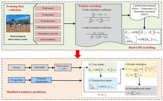
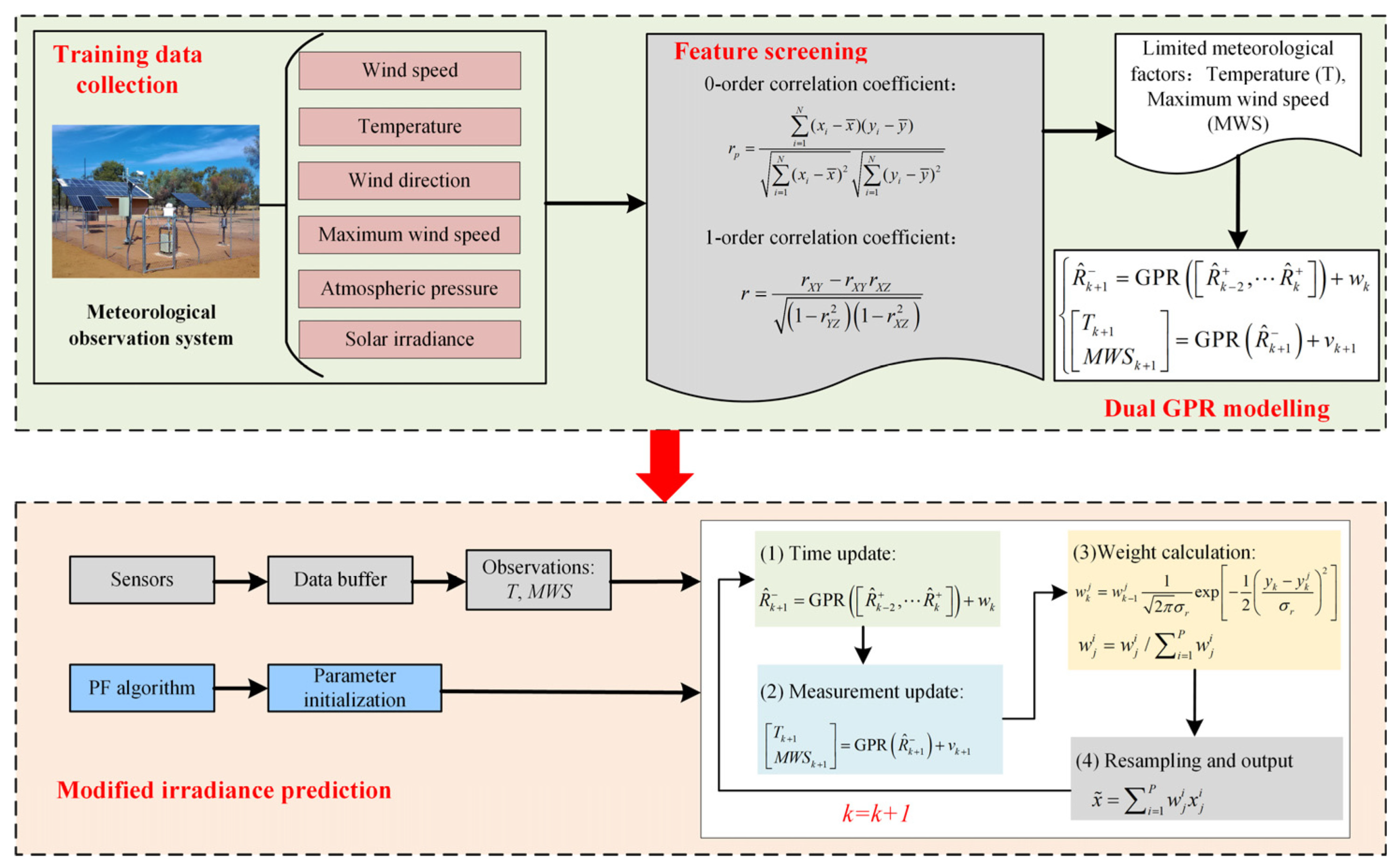
This subsection describes the overall framework for solar irradiance forecasting based on the methodology stated above, as illustrated in Figure 1. The forecasting process is divided into two steps: offline data processing and modeling and real-time irradiance forecasting. The specific steps are as follows. First, in the offline modeling stage, (1) the meteorological observation system collects various historical meteorological factors through sensors for modeling; (2) based on the collected historical data, meteorological factors highly correlated with solar irradiance are identified using multi-layer correlation analysis; (3) from these factors, a limited set is selected for system modeling; (4) using historical solar irradiance data and the selected meteorological factors, GPR is used to establish a dual GPR model describing irradiance variation characteristics. In the online forecasting stage, (5) the meteorological factors are collected in real time by sensors, and the PF algorithm is initialized; (6) the predicted and measured irradiance values of each particle are determined through the time update and measurement update steps; (7) the real-time meteorological observations collected by the sensors are introduced to calculate the particle weight distribution; (8) by weighting the predicted values of each particle, the solar irradiance forecast corrected using the meteorological factors is obtained. (9) Finally, the process advances to the next time step, and steps (5)–(8) are repeated.

Figure 1. The implementation steps of the proposed solar irradiance forecasting method.

3. Experiments and Discussion

3.1. Evaluation Indicator

To evaluate the accuracy of the proposed method and compare the performance of different models, three error metrics are used in this work: mean absolute error (MAE), root mean square error (RMSE), and the R² coefficient. MAE measures the average magnitude of the forecasting errors relative to the observed values and is relatively robust to the influence of outliers. However, it is less sensitive to large errors and does not fully reflect their distribution. Therefore, RMSE is also used to characterize the distribution of forecasting errors, with smaller values indicating better model performance. In addition, the R² coefficient is a statistical metric used to evaluate the goodness of fit of a regression model. Specifically, the above metrics are calculated as follows:

$$\mathrm{MAE}={\displaystyle \frac{1}{n}}{\displaystyle \sum _{i=1}^n\left|y_i-{\widehat{y}}_i\right|}$$

(24)

$$\mathrm{RMSE}=\sqrt{{\displaystyle \frac{1}{n}}{\displaystyle \sum _{i=1}^n{\left(y_i-{\widehat{y}}_i\right)}^2}}$$

(25)

$$R^2=1-{\displaystyle \frac{{\displaystyle \sum _{i=1}^n{\left(y_i-{\widehat{y}}_i\right)}^2}}{{\displaystyle \sum _{i=1}^n{\left(y_i-\overline{y}\right)}^2}}}$$

(26)

where n is the sample size; $y_i$ is the actual value; ${\widehat{y}}_i$ is the prediction of the model; $\overline{y}$ is the mean of the actual values.

3.2. Correlation Analysis of Meteorological Factors

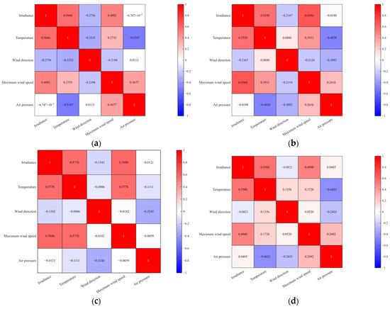
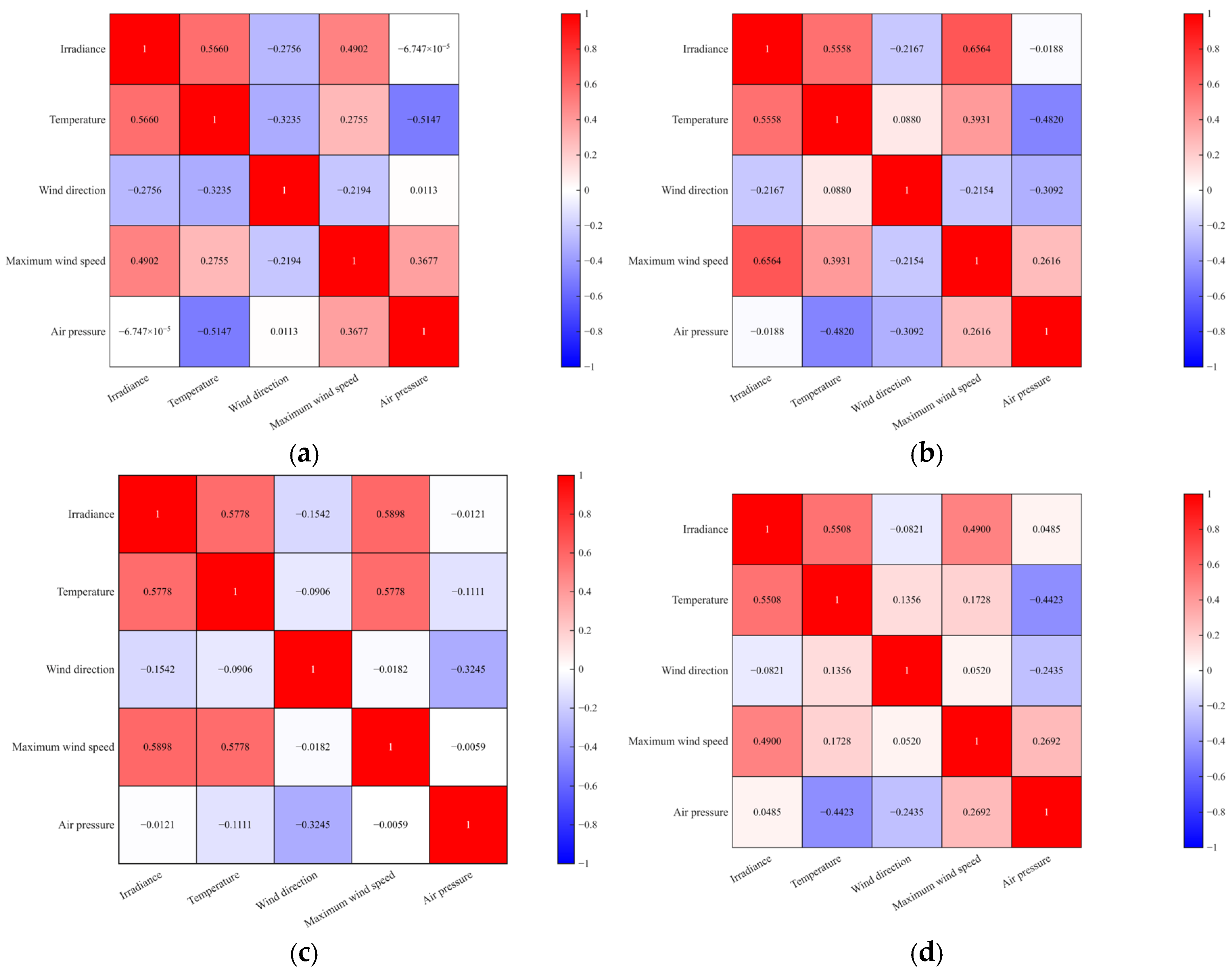
The dataset includes the following meteorological factors: maximum wind speed, ambient temperature, global horizontal radiation, wind direction, and atmospheric pressure. These factors exhibit different degrees of correlation with solar irradiance. Using highly correlated factors to forecast solar irradiance can improve accuracy and further reduce the computational burden of the model. To evaluate the solar irradiance forecasting performance of the proposed method across different seasons, January, April, July, and October are selected as representative months corresponding to the four seasons, respectively. Firstly, the zero-order correlation coefficients between the different meteorological factors and solar irradiance are calculated and presented as heat maps. The resulting coefficients are shown in Figure 2.

Figure 2. Correlation heat map of meteorological factors: (a) January. (b) April. (c) July. (d) October.

As shown in Figure 2, the correlation patterns are generally consistent across the different months of the year, with temperature and maximum wind speed showing the strongest correlations with solar irradiance. Specifically, the descending order of correlation coefficients for January and October is temperature, maximum wind speed, wind direction, and air pressure. For April and July, the correlation coefficient of maximum wind speed exceeds temperature, followed by wind direction and air pressure. The correlations of wind direction and air pressure with solar irradiance are very low throughout the year and much lower than those of the other meteorological factors, indicating their limited ability to reflect changes in irradiance. In addition, the correlation coefficient of maximum wind speed is the greatest during autumn and winter. In spring and summer, when the temperature is relatively high, temperature shows a stronger correlation than maximum wind speed and becomes the most effective meteorological factor for mapping irradiance. Based on the correlation analysis, factors showing strong correlations are selected as preliminary inputs to the forecasting model. Therefore, according to the results in Figure 2, temperature and maximum wind speed are pre-selected as the correction parameters for the forecasting model in this paper.

After selecting highly correlated meteorological factors through the zero-order correlation analysis, we further consider first-order correlations to account for coupling among meteorological variables. The zero-order correlation analysis identifies wind direction and air pressure as weakly correlated factors; these two variables are therefore used separately as control variables to calculate the correlation coefficients between the pre-selected factors and solar irradiance. The specific first-order correlation coefficient calculation results are presented in Table 3.

Table 3. First-order partial correlation coefficient results.

Statistical Index	Month	Control Variable	Temperature	Maximum Wind Speed
First-order correlation coefficient	January	Wind direction	0.5243	0.4582
		Air pressure	0.6601	0.5272
	April	Wind direction	0.5911	0.6396
		Air pressure	0.6241	0.6853
	July	Wind direction	0.5730	0.5942
		Air pressure	0.5801	0.5898
	October	Wind direction	0.5691	0.4966
		Air pressure	0.6388	0.4958

As shown in Table 3, the correlation coefficient for maximum wind speed remains almost unchanged when either wind direction or air pressure is controlled, and wind direction also has little influence on the correlation with temperature. In January, April, and October, when the control variable is air pressure, the correlation coefficient of temperature increases slightly, but the change is not substantial. Overall, the changes in first-order correlation coefficients are small and acceptable. Through the above two-step correlation analysis, it can be determined that selecting temperature and maximum wind speed as the final correction parameters of the irradiance forecasting model is reasonable and well supported.

3.3. Forecasting Results and Discussion

In this section, the proposed method is used to forecast solar irradiance using the selected meteorological factors. Solar irradiance and meteorological data from 2017 are used to test the model, with a measurement interval of 5 min, and the temperature and maximum wind speed are used as correction parameters. Data from four representative months (January, April, July, and October) are used to evaluate the effectiveness of the proposed method across different seasons. For each month, data from the first week are used to train the model, and data from the following week are used for testing. In addition, to evaluate the forecasting accuracy of the proposed method, several commonly used models, including LSTM, bi-directional long short-term memory (BiLSTM), CNN-LSTM, gated recurrent unit (GRU) and temporal convolutional network (TCN), are compared with the proposed method.

For LSTM, BiLSTM, CNN-LSTM, GRU, TCN, and the proposed DGPR-PF model, the network architecture, number of hidden units/layers, optimizer, learning rate, number of training epochs, and other relevant hyperparameters are reported. Note that all the model ML model hyperparameters were set to their default values, and no specific parameter customization was performed for any model to ensure a fair comparison. Specifically, the parameter settings for all ML models are provided in Table 4. In addition, the number of particles in the PF algorithm is N_p = 100.

Table 4. Benchmark models and implementation settings.

Benchmark Models	Implementation Settings
LSTM; BiLSTM; GRU	Hidden units = 100; Dropout rate = 0.2; Learning rate = 0.005; Maximum epochs = 200; Optimizer = Adam.
CNN-LSTM	CNN filters = 2; Kernel size = 3 × 3; LSTM hidden units = 100; Dropout rate = 0.2; Learning rate = 0.005; Maximum epochs = 200; Optimizer = Adam.
TCN	Convolutional filters = [7, 4]; Kernel sizes = [4, 2]; Residual blocks = 1; Dilation factor = 1; Dropout rate = 0.2; Learning rate = 0.005; Maximum epochs = 200; Optimizer = Adam.
GPR	Basis functions = Pure quadratic; Fitting method = Exact; Prediction method = Exact; Hyperparameter optimization = Default.

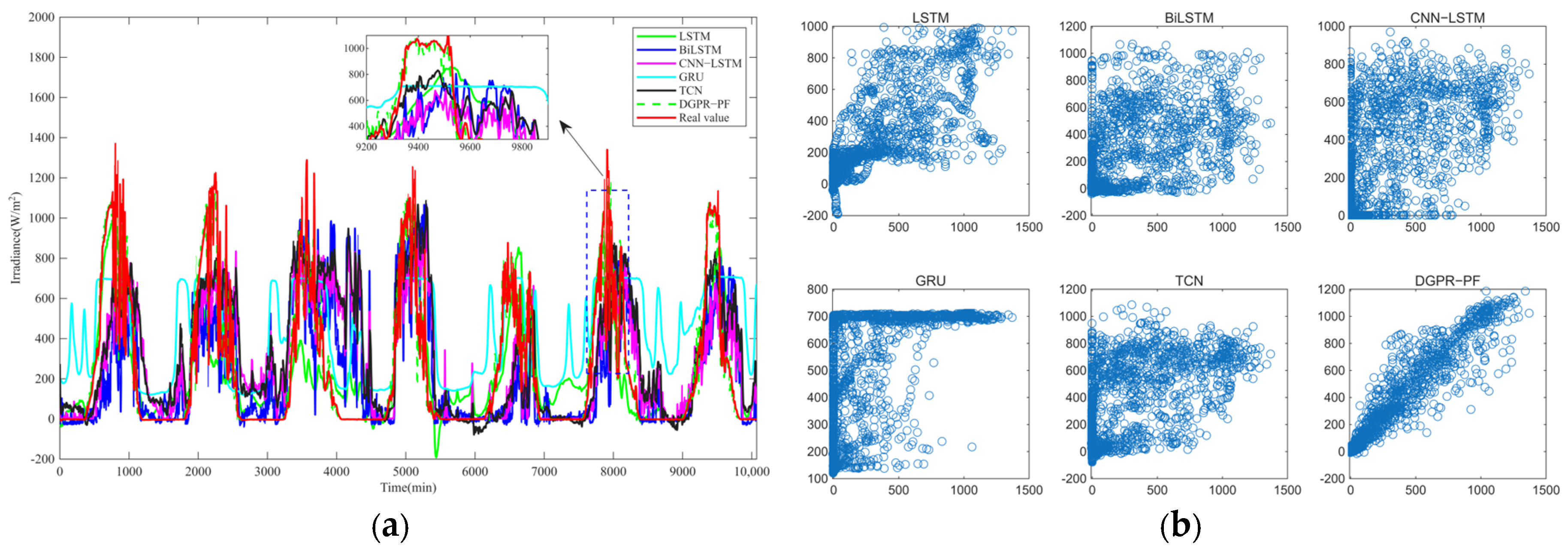
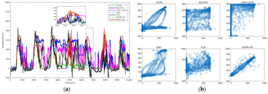
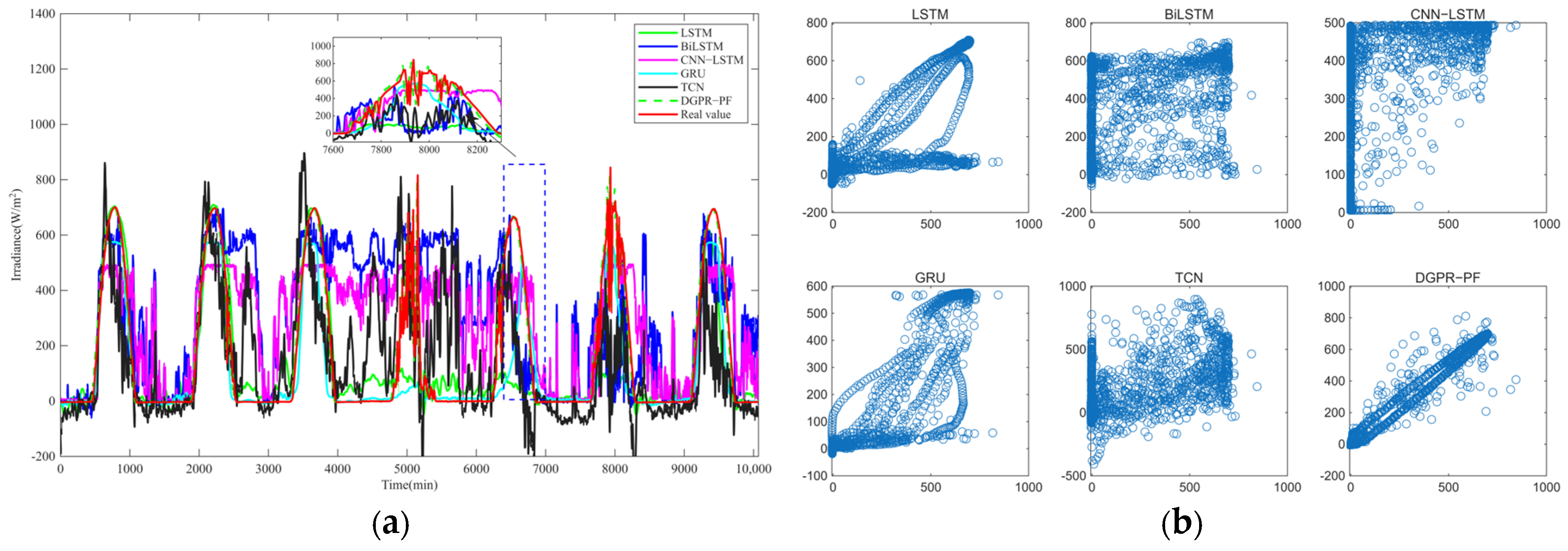
Figure 3 displays the solar irradiance forecasts and regression curves for January. Solar irradiance exhibits substantial daytime fluctuations, including sharp increases and decreases and large variations in amplitude. Among the compared models, GRU shows the poorest overall performance, while BiLSTM provides better forecasting accuracy over the full day. Focusing on daytime irradiance, the detailed results show that the proposed DGPR-PF method more closely tracks fluctuations in the observed values, including fine-scale variations. In contrast, the other methods show larger discrepancies from the observed values in both overall forecasts and detailed variations. In the regression plots, the results of the proposed method are more closely concentrated around the central axis, whereas those of the other methods show greater dispersion, indicating higher forecasting accuracy for the proposed method.

Figure 3. Solar irradiance forecasting results for January: (a) Forecasting result. (b) Comparison between predicted and true values.

Figure 4 shows the irradiance forecasting results for April. Overall, daytime irradiance exhibits relatively small fluctuations and changes smoothly on most days. Moreover, the forecasting curves of LSTM, TCN, and DGPR-PF are relatively close to the observed values, with DGPR-PF showing the closest alignment. LSTM and TCN have similar numerical performance, although the forecasting curve of LSTM is smoother and better reflects the characteristics of the observed values than that of TCN. In the regression plots, the results of the proposed method show a more concentrated distribution, whereas GRU exhibits poorer regression performance.

Figure 4. Solar irradiance forecasting results for April: (a) Forecasting result. (b) Comparison between predicted and true values.

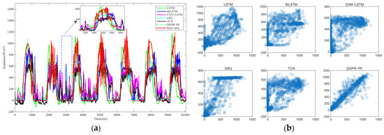
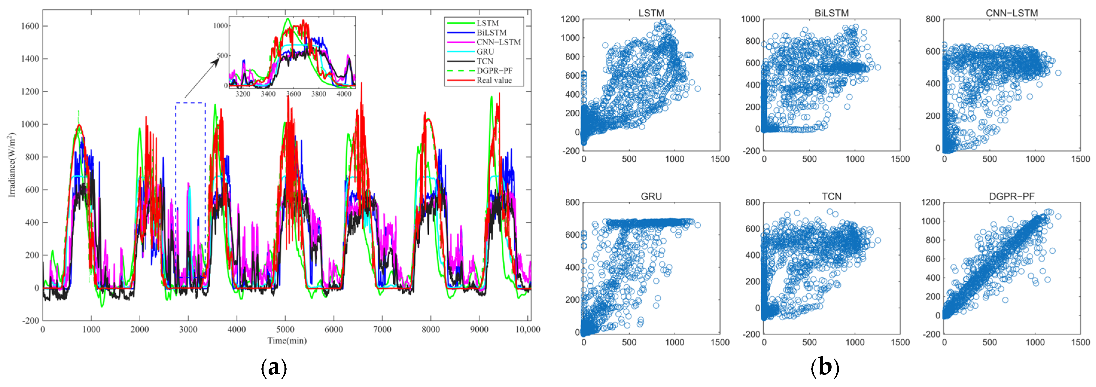
As shown in Figure 5, the forecasting results of TCN and CNN-LSTM for nighttime irradiance are clearly overestimated and inconsistent with the actual behavior of solar irradiance. Their daytime forecasts also differ significantly from the observed values. The forecasting result of GRU is the best among the five compared methods. However, the regression plot in Figure 5b shows that the GRU points are more widely distributed around the central axis than those of DGPR-PF, with some deviation in the overall regression trend.

Figure 5. Solar irradiance forecasting results for July: (a) Forecasting result. (b) Comparison between predicted and true values.

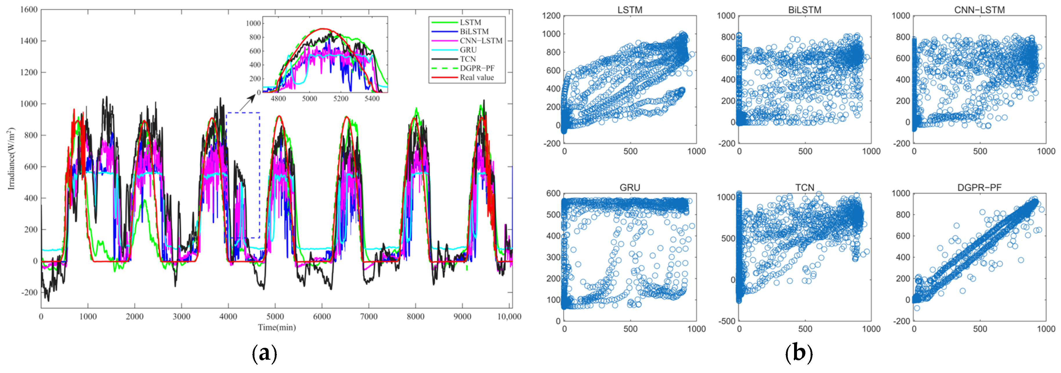
Figure 6 shows that the forecasting results of different models for October are the best among the four datasets. Although the daytime irradiance fluctuates sharply, the forecasts are relatively accurate, especially those of LSTM and DGPR-PF. The detailed forecasting results show that BiLSTM, CNN-LSTM, and TCN exhibit similar numerical accuracy and ability to capture fluctuations. The forecasting results of GRU are less volatile, but the model does not accurately capture continuous fluctuations in solar irradiance caused by external factors and unknown interference. In contrast, DGPR-PF shows the best performance, surpassing LSTM. These results are also reflected in the regression plots, where the forecasts of the proposed method more closely match the observed distribution.

Figure 6. Solar irradiance forecasting results for October: (a) Forecasting result. (b) Comparison between predicted and true values.

Table 5 shows the different error indicators of the proposed method and the comparison method. Combined with the forecasting results, the forecasting performance of solar irradiance is comprehensively analyzed, and the following important conclusions can be drawn:

Table 5. Error indicators comparison results.

Methods	Evaluation Indicators	January	April	July	October
LSTM	MAE (W/m2)	142.87	105.89	91.73	136.31
	RMSE (W/m2)	212.66	165.06	167.98	197.58
	R2	0.622	0.769	0.544	0.690
BiLSTM	MAE (W/m2)	195.63	151.47	228.01	160.20
	RMSE (W/m2)	301.21	244.94	308.56	237.53
	R2	0.242	0.492	0.053	0.552
CNN-LSTM	MAE (W/m2)	202.53	173.44	182.14	194.95
	RMSE (W/m2)	286.26	255.81	236.34	256.22
	R2	0.315	0.446	0.099	0.479
GRU	MAE (W/m2)	273.06	201.54	69.67	92.98
	RMSE (W/m2)	323.77	263.34	134.23	156.73
	R2	0.124	0.4137	0.709	0.805
TCN	MAE (W/m2)	217.21	200.09	146.19	190.51
	RMSE (W/m2)	295.93	293.51	212.23	249.00
	R2	0.268	0.271	0.273	0.508
DGPR-PF	MAE (W/m2)	49.60	22.41	20.55	39.43
	RMSE (W/m2)	99.73	45.14	46.38	85.75
	R2	0.917	0.982	0.965	0.941

(1)

The proposed DGPR-PF can more effectively track the uncertain change trend of solar irradiance, simultaneously, its MAEs are controlled within 100 W/m², and the MAE of other methods are between 100 W/m²–300 W/m². The MAE of the proposed method is much smaller than that of other methods, indicating that the proposed method has higher precision regarding the overall forecasting performance.

(2)

In contrast, the path predicted by DGPR-PF is closer to the real change path, the proposed method not only has a smaller overall error, but also has a more prominent RMSE performance index. The maximum RMSE of the proposed method is 99.73 W/m², indicating that the deviation degree its error is small, that is, the error is mainly concentrated in a small range without extreme forecasting, and the forecasting performance is more stable and reliable. Therefore, the proposed method demonstrates relatively stable performance across the evaluated seasonal datasets.

(3)

The proposed DGPR-PF framework achieves R² values of 0.917, 0.982, 0.965, and 0.941 for January, April, July, and October, respectively, indicating consistently high agreement between the estimated and measured irradiance values. In comparison, the highest R² value among the benchmark models is 0.805, achieved by GRU in October.

(4)

Furthermore, the proposed method achieves an average MAE of 33.00 W/m² and an average RMSE of 69.25 W/m² across the four representative months. Among the five benchmark models, LSTM exhibits the lowest average MAE of 119.20 W/m². Compared with LSTM, the proposed DGPR-PF framework reduces the average MAE by approximately 72.3%. These results demonstrate that the proposed method achieves lower prediction errors than the evaluated benchmark models under the experimental conditions considered.

Specifically, previous studies [43,44] have reported RMSE values ranging from approximately 18.85 W/m² to 89.91 W/m² for LSTM and from 20.75 W/m² to 89.77 W/m² for GRU under different seasonal conditions. In comparison, the proposed DGPR-PF framework achieves RMSE values between 45.14 W/m² and 99.73 W/m² across the four representative months. Above results are generally within the same order of magnitude as those reported in the aforementioned studies. This comparison indicates that the prediction accuracy achieved by the proposed framework is broadly consistent with the error levels reported in the existing literature.

However, differences in meteorological conditions, forecasting horizons, and experimental configurations prevent a direct ranking of the methods across independent studies. These findings provide an external reference for interpreting the present results, while the controlled comparisons within this study demonstrate the effectiveness of the proposed framework. To sum up, the proposed DGPR model combined with PF has better performance in solar irradiance forecasting with limited meteorological factor acquisition. Therefore, the proposed DGPR-PF method can have potential application capability in the real world where fewer measuring equipment are used, and reduce the utilization rate of hardware equipment and save operation equipment cost by means of incremental software algorithm design, thus extending the application of machine learning methods in solar irradiance forecasting.

3.4. Sensitivity Analysis of the Model

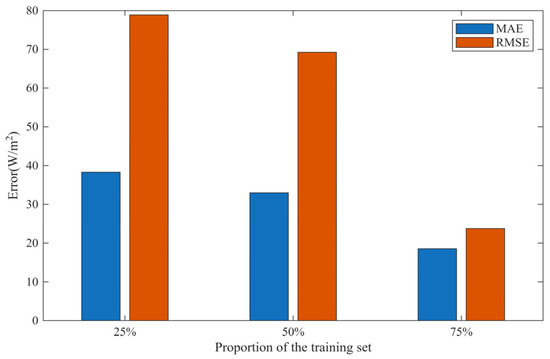
Evaluating the sensitivity of the proposed model to the amount of training data is important, particularly because GPR performance and computational cost are both related to the number of training samples. Therefore, an additional sensitivity analysis is conducted by varying the proportion of training data. Specifically, three training proportions, namely 25%, 50%, and 75%, were considered to investigate the influence of training sample size on prediction accuracy. The corresponding results, evaluated using MAE and RMSE, are presented in Figure 7.

Figure 7. Error analysis of training sets with different proportions.

The experimental results indicate that increasing the amount of training data consistently improves the prediction accuracy of the proposed framework. When the training proportion increases from 25% to 50%, the MAE decreases from approximately 38.2 W/m² to 33.0 W/m², while the RMSE decreases from approximately 79.0 W/m² to 69.2 W/m². When the training proportion further increases to 75%, the MAE and RMSE decrease to approximately 18.5 W/m² and 23.9 W/m², respectively. Compared with the 25% training proportion, these results correspond to reductions of approximately 52% in MAE and 70% in RMSE.

The observed improvement can be explained by the increased amount of training information available to the GPR models. A larger training dataset allows the state-transition GPR to capture the temporal variations in solar irradiance more accurately, while the observation GPR models can better characterize the nonlinear relationships between irradiance and meteorological variables. These improvements provide more reliable inputs to the subsequent particle filtering process, thereby reducing the overall estimation errors. These additional results confirm that the proposed DGPR-PF framework is sensitive to training sample size, with improved accuracy as more training data become available. At the same time, the results provide quantitative evidence of the model’s behavior under limited-data conditions.

3.5. Computational Complexity Analysis of Different Models

Computational complexity and execution efficiency are essential considerations when evaluating the practical applicability of forecasting models, particularly for real-time solar irradiance prediction. In addition, we implement a theoretical computational complexity analysis and experimentally compare the total computational time (including training and forecasting times) of different methods, including LSTM, BiLSTM, CNN-LSTM, GRU, TCN, and the proposed DGPR-PF framework. The corresponding results are presented in Table 6.

Table 6. Computational efficiency comparison of different forecasting methods.

Method	Total Time (s)
LSTM	11.31
BiLSTM	38.73
CNN-LSTM	36.24
GRU	33.23
TCN	13.96
Proposed DGPR-PF	36.58

Specifically, the total time of LSTM, BiLSTM, CNN-LSTM, GRU, and TCN are 11.31 s, 38.73 s, 36.24 s, 33.23 s, and 13.96 s, respectively, while the proposed DGPR-PF framework requires 36.58 s. These results indicate that the proposed framework has a computational efficiency comparable to CNN-LSTM and approximately 5.6% lower than BiLSTM. Although its forecasting time is higher than those of LSTM, GRU, and TCN, the additional computational burden remains moderate under the investigated experimental conditions.

Regarding theoretical complexity, it is reported that exact GPR training requires O(N³) computational operations and O(N²) memory, where N denotes the number of training samples. The proposed framework employs two independently trained GPR regressors, including one state-transition model and observation models. Therefore, its overall training complexity remains O(N³) when the two training sample sizes are of the same order. For online estimation, the computational burden is primarily associated with evaluating the GPR models for individual particles and performing particle resampling. Assuming O(N) complexity for each GPR predictive mean, the online computational complexity is approximately O(N_p × N + N_p²) per time step for the current implementation, where N_p denotes the number of particles. The O(N_p²) term is associated with the nested-loop multinomial resampling procedure. In our experiments, the particle number is set to 100, which helps limit the computational cost of sequential estimation.

It is also important to distinguish offline model training from online prediction. Once the GPR models have been trained, their hyperparameters and associated model quantities can be reused during sequential estimation without retraining at every time step. Consequently, the training complexity does not directly represent the computational cost of each online prediction. Nevertheless, we acknowledge that the proposed framework does not necessarily provide the lowest computational cost among the evaluated methods. In particular, the training complexity of exact GPR may become a limitation when the number of training samples increases substantially. Moreover, the measured training times alone are insufficient to establish the real-time superiority of the proposed framework over LSTM or GRU, which can perform efficient inference after training.

4. Conclusions

Due to regional and operational constraints, the meteorological data available at different photovoltaic power stations vary. Developing a reliable model that can accurately forecast solar irradiance using limited meteorological parameters from an incomplete weather measurement system remains challenging. To address this problem, we propose a dual GPR-PF framework combined with a correction method using limited meteorological factors for short-term solar irradiance forecasting. The experimental results demonstrate the forecasting performance of the proposed method, and the key conclusions can be summarized as follows: (1) The use of a multi-layer correlation analysis to screen meteorological factors enables effective analysis of the relationships among relevant variables while accounting for their coupling. (2) A dual GPR-PF framework is developed to describe the variation characteristics and influencing factors of solar irradiance. The dual GPR model improves forecasting stability and suppresses measurement noise. (3) The Yulara Solar System dataset in Australia is used to validate the proposed method under different seasonal conditions and to compare its performance with commonly used methods. The results show that the proposed method achieves high forecasting accuracy and reliability through model updating and correction using meteorological factors. The maximum MAE and RMSE are 49.60 W/m² and 99.73 W/m², respectively, and the model demonstrates a stronger goodness of fit.

References

- Michael, N.E.; Hasan, S.; Al-Durra, A.; Mishra, M. Short-term solar irradiance forecasting based on a novel Bayesian optimized deep Long Short-Term Memory neural network. Appl. Energy 2022, 324, 119727. [Google Scholar] [CrossRef] [Scilit]
- Lou, S.; Li, D.H.; Lam, J.C.; Chan, W.W. Prediction of diffuse solar irradiance using machine learning and multivariable regression. Appl. Energy 2016, 181, 367–374. [Google Scholar] [CrossRef] [Scilit]
- Cheng, H.Y.; Yu, C.C.; Lin, C.L. Day-ahead to week-ahead solar irradiance prediction using convolutional long short-term memory networks. Renew. Energy 2021, 179, 2300–2308. [Google Scholar] [CrossRef] [Scilit]
- Cheng, H.Y.; Yu, C.C.; Lin, S.J. Bi-model short-term solar irradiance prediction using support vector regressors. Energy 2014, 70, 121–127. [Google Scholar] [CrossRef] [Scilit]
- Alhamrouni, I.; Abdul Kahar, N.H.; Salem, M.; Swadi, M.; Zahroui, Y.; Kadhim, D.J.; Mohamed, F.A.; Alhuyi Nazari, M. A Comprehensive Review on the Role of Artificial Intelligence in Power System Stability, Control, and Protection: Insights and Future Directions. Appl. Sci. 2024, 14, 6214. [Google Scholar] [CrossRef] [Scilit]
- Lee, J.; Wang, W.; Harrou, F.; Sun, Y. Reliable solar irradiance prediction using ensemble learning-based models: A comparative study. Energy Convers. Manag. 2020, 208, 112582. [Google Scholar] [CrossRef] [Scilit]
- Dong, N.; Chang, J.F.; Wu, A.G.; Gao, Z.K. A novel convolutional neural network framework based solar irradiance prediction method. Int. J. Electr. Power Energy Syst. 2020, 114, 105411. [Google Scholar] [CrossRef] [Scilit]
- Gutierrez-Corea, F.V.; Manso-Callejo, M.A.; Moreno-Regidor, M.P.; Manrique-Sancho, M.T. Forecasting short-term solar irradiance based on artificial neural networks and data from neighboring meteorological stations. Sol. Energy 2016, 134, 119–131. [Google Scholar] [CrossRef] [Scilit]
- Kumari, P.; Toshniwal, D. Deep learning models for solar irradiance forecasting: A comprehensive review. J. Clean. Prod. 2021, 318, 128566. [Google Scholar] [CrossRef] [Scilit]
- Xiu-Yan, G.; Jie-Mei, L.; Yuan, Y.; He-Ping, T. Global horizontal irradiance prediction model considering the effect of aerosol optical depth based on the Informer model. Renew. Energy 2024, 220, 119671. [Google Scholar] [CrossRef] [Scilit]
- Xie, Q.; Ma, L.; Liu, Y.; Fu, Q.; Shen, Z.; Wang, X. An improved SSA-BiLSTM-based short-term irradiance prediction model via sky images feature extraction. Renew. Energy 2023, 219, 119507. [Google Scholar] [CrossRef] [Scilit]
- Ssekulima, E.B.; Anwar, M.B.; Al Hinai, A.; El Moursi, M.S. Wind speed and solar irradiance forecasting techniques for enhanced renewable energy integration with the grid: A review. IET Renew. Power Gener. 2016, 10, 885–989. [Google Scholar]
- Puah, B.K.; Chong, L.W.; Wong, Y.W.; Begam, K.M.; Khan, N.; Juman, M.A.; Rajkumar, R.K. A regression unsupervised incremental learning algorithm for solar irradiance prediction. Renew. Energy 2021, 164, 908–925. [Google Scholar] [CrossRef] [Scilit]
- Li, J.; Ward, J.K.; Tong, J.; Collins, L.; Platt, G. Machine learning for solar irradiance forecasting of photovoltaic system. Renew. Energy 2016, 90, 542–553. [Google Scholar] [CrossRef] [Scilit]
- Huang, X.; Li, Q.; Tai, Y.; Chen, Z.; Zhang, J.; Shi, J.; Gao, B.; Liu, W. Hybrid deep neural model for hourly solar irradiance forecasting. Renew. Energy 2021, 171, 1041–1060. [Google Scholar] [CrossRef] [Scilit]
- Gao, B.; Huang, X.; Shi, J.; Tai, Y.; Zhang, J. Hourly forecasting of solar irradiance based on CEEMDAN and multi-strategy CNN-LSTM neural networks. Renew. Energy 2020, 162, 1665–1683. [Google Scholar] [CrossRef] [Scilit]
- Golam, M.; Akter, R.; Lee, J.M.; Kim, D.S. A long short-term memory-based solar irradiance prediction scheme using meteorological data. IEEE Geosci. Remote Sens. Lett. 2021, 19, 1–5. [Google Scholar] [CrossRef] [Scilit]
- Michael, N.E.; Bansal, R.C.; Ismail, A.A.; Elnady, A.; Hasan, S. A cohesive structure of Bi-directional long-short-term memory (BiLSTM)-GRU for predicting hourly solar radiation. Renew. Energy 2024, 222, 119943. [Google Scholar] [CrossRef] [Scilit]
- Hou, X.; Ju, C.; Wang, B. Prediction of solar irradiance using convolutional neural network and attention mechanism-based long short-term memory network based on similar day analysis and an attention mechanism. Heliyon 2023, 9, e21484. [Google Scholar] [CrossRef] [Scilit]
- Wang, Z.; Wang, F.; Su, S. Solar irradiance short-term prediction model based on BP neural network. Energy Procedia 2011, 12, 488–494. [Google Scholar] [CrossRef] [Scilit]
- Angstrom, A. Solar and terrestrial radiation. Report to the international commission for solar research on actinometric investigations of solar and atmospheric radiation. Q. J. R. Meteorol. Soc. 1924, 50, 121–126. [Google Scholar] [CrossRef] [Scilit]
- Jalali, S.M.J.; Ahmadian, S.; Nakisa, B.; Khodayar, M.; Khosravi, A.; Nahavandi, S.; Islam, S.M.S.; Shafie-Khah, M.; Catalão, J.P. Solar irradiance forecasting using a novel hybrid deep ensemble reinforcement learning algorithm. Sustain. Energy Grids Netw. 2022, 32, 100903. [Google Scholar] [CrossRef] [Scilit]
- Bae, K.Y.; Jang, H.S.; Sung, D.K. Hourly solar irradiance prediction based on support vector machine and its error analysis. IEEE Trans. Power Syst. 2016, 32, 935–945. [Google Scholar] [CrossRef] [Scilit]
- Maciel, J.N.; Ledesma, J.J.G.; Junior, O.H.A. Hybrid prediction method of solar irradiance applied to short-term photovoltaic energy generation. Renew. Sustain. Energy Rev. 2024, 192, 114185. [Google Scholar] [CrossRef] [Scilit]
- Huang, X.; Liu, J.; Xu, S.; Li, C.; Li, Q.; Tai, Y. A 3D ConvLSTM-CNN network based on multi-channel color extraction for ultra-short-term solar irradiance forecasting. Energy 2023, 272, 127140. [Google Scholar] [CrossRef] [Scilit]
- Zang, H.; Zhang, Y.; Cheng, L.; Ding, T.; Wei, Z.; Sun, G. Multi-site solar irradiance forecasting based on adaptive spatiotemporal graph convolutional network. Expert Syst. Appl. 2024, 236, 121313. [Google Scholar] [CrossRef] [Scilit]
- Wang, H.; Cai, R.; Zhou, B.; Aziz, S.; Qin, B.; Voropai, N.; Gan, L.; Barakhtenko, E. Solar irradiance forecasting based on direct explainable neural network. Energy Convers. Manag. 2020, 226, 113487. [Google Scholar] [CrossRef] [Scilit]
- Sibtain, M.; Li, X.; Saleem, S.; Shi, Q.; Li, F.; Saeed, M.; Majeed, F.; Shah, S.S.A.; Saeed, M.H. Multifaceted irradiance prediction by exploiting hybrid decomposition-entropy-Spatiotemporal attention based Sequence2Sequence models. Renew. Energy 2022, 196, 648–682. [Google Scholar] [CrossRef] [Scilit]
- Li, C.; Zhang, Y.; Zhao, G.; Ren, Y. Hourly solar irradiance prediction using deep BiLSTM network. Earth Sci. Inform. 2021, 14, 299–309. [Google Scholar] [CrossRef] [Scilit]
- Kamadinata, J.O.; Ken, T.L.; Suwa, T. Sky image-based solar irradiance prediction methodologies using artificial neural networks. Renew. Energy 2019, 134, 837–845. [Google Scholar] [CrossRef] [Scilit]
- Sharma, V.; Yang, D.; Walsh, W.; Reindl, T. Short term solar irradiance forecasting using a mixed wavelet neural network. Renew. Energy 2016, 90, 481–492. [Google Scholar] [CrossRef] [Scilit]
- Qing, X.; Niu, Y. Hourly day-ahead solar irradiance prediction using weather forecasts by LSTM. Energy 2018, 148, 461–468. [Google Scholar] [CrossRef] [Scilit]
- Kumari, P.; Toshniwal, D. Long short term memory–convolutional neural network based deep hybrid approach for solar irradiance forecasting. Appl. Energy 2021, 295, 117061. [Google Scholar] [CrossRef] [Scilit]
- Zhao, H.; Huang, X.; Xiao, Z.; Shi, H.; Li, C.; Tai, Y. Week-ahead hourly solar irradiation forecasting method based on ICEEMDAN and TimesNet networks. Renew. Energy 2024, 220, 119706. [Google Scholar] [CrossRef] [Scilit]
- Hoyos-Gómez, L.S.; Ruiz-Muñoz, J.F.; Ruiz-Mendoza, B.J. Short-term forecasting of global solar irradiance in tropical environments with incomplete data. Appl. Energy 2022, 307, 118192. [Google Scholar] [CrossRef] [Scilit]
- Li, J.; Liu, Q. Forecasting of short-term photovoltaic power generation using combined interval type-2 Takagi-Sugeno-Kang fuzzy systems. Int. J. Electr. Power Energy Syst. 2022, 140, 108002. [Google Scholar] [CrossRef] [Scilit]
- DKASC. Yulara Solar System; OmniScriptum: London, UK, 2021. [Google Scholar]
- Sharma, N.; Mangla, M.; Yadav, S.; Goyal, N.; Singh, A.; Verma, S.; Saber, T. A sequential ensemble model for photovoltaic power forecasting. Comput. Electr. Eng. 2021, 96, 107484. [Google Scholar] [CrossRef] [Scilit]
- Acikgoz, H. A novel approach based on integration of convolutional neural networks and deep feature selection for short-term solar radiation forecasting. Appl. Energy 2022, 305, 117912. [Google Scholar] [CrossRef] [Scilit]
- Yu, Y.; Yao, X.; Tang, Y.; Yang, L. Hourly global radiation modified model based on meteorological elements-a case study of Xi’an. Acta Energiae Solaris Sin. 2023, 44, 15–21. [Google Scholar]
- Chen, Y.; Dong, Z.; Su, J.; Wang, Y.; Han, Z.; Zhou, D.; Zhao, Y.; Bao, Y. Framework of airfoil max lift-to-drag ratio prediction using hybrid feature mining and Gaussian process regression. Energy Convers. Manag. 2021, 243, 114339. [Google Scholar] [CrossRef] [Scilit]
- He, N.; Qian, C.; Li, R.; Zhang, M. An improved pipeline leak detection and localization method based on compressed sensing and event-triggered particle filter. J. Frankl. Inst. 2021, 358, 8085–8108. [Google Scholar] [CrossRef] [Scilit]
- Yan, K.; Shen, H.; Wang, L.; Zhou, H.; Xu, M.; Mo, Y. Short-term solar irra-diance forecasting based on a hybrid deep learning methodology. Information 2020, 11, 32. [Google Scholar] [CrossRef] [Scilit]
- Elmousaid, R.; Drioui, N.; Elgouri, R.; Agueny, H.; Adnani, Y. Ul-tra-short-term global horizontal irradiance forecasting based on a novel and hybrid GRU-TCN model. Results Eng. 2024, 23, 102817. [Google Scholar] [CrossRef] [Scilit]
Disclaimer/Publisher’s Note: The statements, opinions and data contained in all publications are solely those of the individual author(s) and contributor(s) and not of MDPI and/or the editor(s). MDPI and/or the editor(s) disclaim responsibility for any injury to people or property resulting from any ideas, methods, instructions or products referred to in the content. |
© 2026 by the authors. Licensee MDPI, Basel, Switzerland. This article is an open access article distributed under the terms and conditions of the Creative Commons Attribution (CC BY) license.