


Abstract
Doubly Fed Induction Generator (DFIG)-based Wind Energy Conversion Systems (WECSs) rely on accurate sensor measurements to ensure stable operation and effective power conversion. However, sensor faults can compromise control performance and system reliability and lead to unscheduled shutdowns if they are not promptly detected and accommodated. This paper presents an Active Fault-Tolerant Control (AFTC) framework for a grid-connected DFIG-based WECS, integrating an existing sensor Fault Detection and Isolation (FDI) methodology with a novel control reconfiguration framework. The inherited FDI module detects and isolates sensor faults, while the proposed reconfiguration framework automatically selects an appropriate compensation strategy according to the number of simultaneously faulty sensors. Pure Measurement Compensation (PMC), Hybrid Measurement-Estimation Compensation (HMEC), and Pure Estimation Compensation (PEC) are employed for single-, double-, and triple-sensor fault scenarios, respectively. These strategies replace or reconstruct faulty sensor measurements within the affected control loops using available healthy or estimated signals. The proposed framework is implemented in MATLAB/Simulink and evaluated under additive and multiplicative sensor fault scenarios. The decision function reaches the detection threshold approximately ms after fault injection, while the effective fault identification and isolation signal is activated within approximately ms, followed by the activation of the corresponding compensation strategy. The simulation results demonstrate that the proposed reconfiguration strategies for the AFTC framework maintain continuous converter operation and satisfactory dynamic performance following fault diagnosis. The proposed framework provides a structured approach to active control reconfiguration for improved reliability and resilience to faults in DFIG-based WECSs.
1. Introduction
The progressive depletion of global fossil fuel reserves, the deterioration of environmental conditions, and the increasing demand for sustainable energy have intensified global efforts toward clean and renewable energy sources (RESs) to achieve a low-carbon economy [1,2,3,4]. Among various RESs, wind energy has emerged as one of the most promising alternatives due to its technical maturity, high energy conversion efficiency, large-scale industrial deployment, and substantial socioeconomic benefits [3,4,5,6,7]. Consequently, wind power is steadily contributing a growing share to the global energy market [8,9,10]. Over the years, three generations of wind turbine (WT) technologies have been deployed in wind farms:
- Fixed-speed WTs directly connected to the grid using a squirrel-cage induction generator (SCIG),
- Variable-speed WTs based on a doubly fed induction generator (DFIG), in which the stator is directly connected to the grid while the rotor is linked through back-to-back converters [4,5,11], and
- Direct-drive variable-speed WTs employing a permanent magnet synchronous generator (PMSG) interfaced with the grid via a variable-frequency power converter [12].
Among these configurations, DFIG-based wind energy conversion systems (WECSs) have become one of the most widely adopted technologies in modern wind farms. Their popularity is attributed to their high efficiency, variable-speed operation, reduced converter rating, cost-effectiveness, and independent control of active and reactive power [4,5,11].
The DFIG configuration employs two converters: the rotor-side converter (RSC) and the grid-side converter (GSC). These converters work together to efficiently regulate power flow between the DFIG and the utility grid. The RSC, connected to the rotor windings, regulates the active and reactive powers at the stator terminals, while the GSC maintains a stable DC-link voltage and ensures compliance with grid standards [4,5,8,11,13]. However, the direct coupling of the DFIG converters to the grid exposes them to grid disturbances and fault conditions [5,14]. Variations in wind speed cause fluctuations in generated power, which must be conditioned by the converters to match the grid’s frequency and voltage requirements [7]. Their operation is governed by dedicated control strategies that regulate the power exchanged between the DFIG and the utility grid. The effectiveness of these control algorithms relies heavily on accurate current and voltage measurements provided by the sensing system [4,14,15]. Consequently, the reliability of sensor measurements is essential for ensuring proper converter operation and maintaining overall system stability. In practice, current and voltage sensors are particularly susceptible to faults caused by harsh operating environments, aging, and electromagnetic interference, making them among the most critical components in DFIG-based WECSs [4,16]. Sensor faults degrade measurement accuracy, compromise current control performance, and may result in partial or complete loss of converter controllability. If left undetected, these faults can propagate throughout the control system, leading to power quality degradation, increased maintenance costs, reduced energy production, and, in severe cases, turbine shutdown and disconnection from the grid [4,14,15,16]. The adverse effects of sensor faults become particularly critical when they compromise converter operation. For instance, GSC voltage regulation may be severely affected, introducing secondary harmonics into the grid voltage and current, perturbing the grid-side active and reactive powers, increasing losses, and destabilizing the DC-link capacitor voltage [8]. Faults can also cause stator current surges, leading to subsequent voltage dips at the generator terminals. Due to magnetic coupling between the stator and rotor circuits, excessive rotor currents may occur, potentially leading to RSC failure. As wind power penetration increases, such events can severely impact overall system stability [7,10].
The continuous growth of wind generation capacity demands more powerful and complex equipment, thereby increasing the need for high reliability and operational dependability [7,9,17]. Most WTs operate under harsh environmental conditions and are subjected to significant mechanical and electrical stresses, making them vulnerable to faults and component degradation. Unplanned shutdowns, performance deterioration, and system failures result in substantial economic losses due to the high operational, maintenance, and reconnection costs associated with WECSs [10,17,18]. Consequently, there is a growing need to improve the operational dependability, availability, and fault resilience of WECSs [7,8,9]. In this context, timely Fault Detection and Isolation (FDI), effective fault management, and the implementation of Fault-Tolerant Control (FTC) strategies are essential for maintaining system performance, reducing economic losses, and ensuring safe and continuous operation [9,14,17,18,19,20,21,22]. FTC enables systems to maintain acceptable performance under fault conditions through timely FDI and control reconfiguration before faults propagate and compromise system stability [9,14,18,20]. Consequently, FTC has attracted considerable research attention and is increasingly being adopted in safety-critical applications requiring high reliability and service continuity [18,20,23].
Numerous control and monitoring strategies have been proposed to improve the performance and reliability of DFIG-based WECSs under varying operating conditions. Although conventional linear control strategies, such as Proportional-Integral (PI) and Proportional-Integral-Derivative (PID) controllers, are widely used due to their simple implementation, they exhibit limited effectiveness in the presence of nonlinear dynamics, model uncertainties, and fault conditions [5,7,11]. To overcome these limitations, several advanced nonlinear and robust control techniques have been developed [5,7,10]. Mosaad [5] proposed a Direct Power Control (DPC) strategy combined with a Fractional-Order PI (FOPI) controller to enhance the integration of DFIG-based WECSs into the electrical grid. More recently, Mosaad [11] introduced an adaptive predictive fuzzy-neural-network controller to maximize the extracted wind power under varying operating conditions. These strategies effectively address the limitations of traditional PID controllers and significantly improve the dynamic performance of WECSs. Nevertheless, these strategies primarily address external fault events, such as grid voltage sags, load disturbances, and sensor noise, rather than internal sensor fault detection and estimation.
To enhance system reliability under fault conditions, numerous FDI techniques have been proposed for DFIG-based WECSs. Kumari and Priya [15] developed a model-based observer combined with fuzzy logic for current sensor fault detection and isolation in DFIG systems. Li et al. [24] presented an adaptive observer-based FDI strategy for wind turbines capable of accurately detecting and isolating sensor faults under varying operating conditions. Subsequently, Li et al. [16] proposed a Sliding-Mode Observer (SMO) based on a novel reaching law to improve fault detection robustness under uncertainties. Abbas et al. [4] proposed an Extended Kalman Filter (EKF) bank capable of detecting both single and multiple current sensor faults with improved diagnostic accuracy under varying operating conditions in DFIG-based WECSs.
Beyond FDI methods, considerable research has focused on FTC strategies to maintain acceptable system performance following fault occurrence. Xiahou et al. [14] proposed an observer-based sensor FTC scheme for DFIG-based WECSs employing three parallel sensor fault observers (SFOs) to estimate and compensate for stator, rotor, and grid current sensor faults. Dong et al. [25] further proposed an adaptive fractional-order sliding-mode FTC strategy for DFIG-based WECSs to improve robustness against parameter uncertainties and external disturbances. To further improve control performance under sensor faults, Ghanbarpour et al. [26] developed an observer-based Model Predictive Control (MPC) strategy for partial-load WT operation, where an SMO was used for fault estimation and compensation. In a subsequent study, Ghanbarpour et al. [27] extended this framework by developing an MPC-based passive FTC scheme capable of simultaneously accommodating both sensor and actuator faults. Furthermore, Teng et al. [17] introduced an adaptive observer-based FTC framework that compensates both sensor and actuator faults while preserving closed-loop stability under varying operating conditions. Similarly, Mohammedi et al. [28] proposed a nonlinear FTC strategy to ensure service continuity of WECSs under fault conditions.
Recent studies have further addressed robustness and FTC operation in electrical drive systems through enhanced observer and post-fault control techniques. In [29], an Enhanced Integral Sliding-Mode Observer (E-ISMO)-based model-free predictive current control method was proposed for dual three-phase permanent magnet synchronous motor (DT-PMSM) drives. The proposed observer improves disturbance estimation accuracy under parameter mismatches and inverter nonlinearities and supports the robustness of the control approach. Similarly, the authors of [30] proposed a Generalized Free-Current-Curve Fault-Tolerant Control (GFCC-FTC) method for arbitrary-phase-shift dual three-phase PMSM systems under open-phase faults. The method exploits greater freedom in current trajectory selection to achieve copper-loss minimization and improved torque capability under post-fault operating conditions. Although these studies primarily focus on disturbance estimation and control robustness rather than sensor fault accommodation, they highlight the importance of reliable observer performance and post-fault control under system uncertainties and nonlinear disturbances.
Although recent studies have investigated integrated fault diagnosis and FTC mechanisms for DFIG-based WECSs, most existing approaches remain dedicated to specific fault categories, fault types, or operating conditions. Furthermore, limited attention has been devoted to integrated FDI–Active FTC frameworks capable of simultaneously handling both additive and multiplicative sensor faults while combining robust fault isolation with effective control reconfiguration. Consequently, the coordinated integration of accurate fault detection, reliable fault isolation, and active FTC reconfiguration remains insufficiently explored for DFIG-based WECSs operating under diverse sensor fault scenarios. These limitations motivate the development of the proposed integrated FDI-based AFTC strategy to ensure continuous and stable operation under sensor fault conditions.
Building upon this motivation, the present study develops an integrated Active Fault-Tolerant Control (AFTC) framework for a grid-connected DFIG-based WECS to accommodate additive and multiplicative sensor faults. The proposed architecture combines an existing sensor Fault Detection and Isolation (FDI) methodology with a novel fault reconfiguration framework designed to improve system robustness against sensor faults while maintaining stable converter operation. The proposed AFTC framework builds upon the validated FDI methodology developed by Beddek et al. [12], which employs the Generalized Observer Scheme (GOS), Time-Variant Kalman Filter (TVKF), Maximum Shift Strategy, and Cumulative Sum (CUSUM)-based decision logic for sensor fault diagnosis. Therefore, the novelty of the present study does not lie in the development of a new FDI algorithm. Instead, the main novelty lies in the development, integration, and validation of an Active FTC based on a novel fault reconfiguration framework that uses the diagnosis information provided by the existing FDI module to accommodate faulty sensor measurements within the DFIG control system. Specifically, three complementary reconfiguration strategies are developed: Pure Measurement Compensation (PMC), Hybrid Measurement-Estimation Compensation (HMEC), and Pure Estimation Compensation (PEC). Depending on the identified faulty sensor and the availability of healthy or estimated measurements, the proposed reconfiguration framework automatically selects an appropriate compensation mechanism to replace or reconstruct the corrupted measurement used by the affected control loop. This enables the DFIG control system to continue operating without directly relying on the faulty sensor signal. The proposed framework is implemented in MATLAB/Simulink R2018a and evaluated under different additive and multiplicative sensor fault scenarios. The assessment focuses on the effectiveness of the proposed reconfiguration strategies in mitigating the effects of diagnosed sensor faults and maintaining satisfactory dynamic performance and continuous converter operation. Thus, the study specifically addresses the fault accommodation stage following FDI, rather than modifying or improving the inherited FDI algorithm.
The main contributions of this paper can be summarized as follows:
- A novel fault reconfiguration framework is developed for the active fault-tolerant control of grid-connected DFIG-based WECS and integrated with the existing FDI methodology of Beddek et al. [12]. The proposed framework establishes the link between diagnosed sensor faults and the subsequent control accommodation process.
- Three complementary control reconfiguration strategies are developed within the proposed framework, namely, Pure Measurement Compensation (PMC), Hybrid Measurement–Estimation Compensation (HMEC), and Pure Estimation Compensation (PEC). These strategies provide alternative mechanisms for replacing or reconstructing faulty sensor measurements within the affected control loops, allowing continued controller operation following sensor faults.
- The proposed reconfiguration framework accommodates both additive and multiplicative sensor faults. Based on the fault information provided by the FDI module, an appropriate reconfiguration strategy is selected according to the identified faulty measurement and the availability of healthy or estimated signals, thereby preventing the corrupted sensor signal from directly affecting the corresponding control loop.
- The integrated FDI-based AFTC framework is implemented in MATLAB/Simulink and systematically evaluated under different sensor fault scenarios. The simulation results assess the effectiveness of the proposed reconfiguration strategies in mitigating the impact of sensor faults and maintaining satisfactory dynamic performance and continuous DFIG-based WECS operation following fault diagnosis.
The rest of this paper is organized as follows: Section 2 gives an overview of the DFIG-based WECS modeling and control; Section 3 discusses fault definitions, classifications, and the fundamentals of FTC, distinguishing between passive and active strategies; Section 4 gives an overall description of a nonsinusoidal three-phase system under balanced conditions; Section 5 presents a detailed description of the integrated FDI-based AFTC model and control implementation; Section 6 reports and analyzes the simulation results; and Section 7 concludes the study with future work directions.
2. Comparison and Novelty
The main distinction of the proposed approach from conventional observer-based sensor fault-tolerant control methods lies in the organization of the post-fault measurement reconstruction process. The proposed framework does not introduce a new observer or a new FDI algorithm; instead, it uses the information supplied by the existing FDI module to automatically select an appropriate compensation mechanism according to the number of simultaneously faulty sensors. For a single sensor fault, PMC exploits the analytical redundancy inherent in the balanced three-phase system and reconstructs the faulty measurement exclusively from the two healthy measurements. When two sensors are faulty, HMEC combines the remaining healthy measurement with the TVKF-based estimates, thereby exploiting both physical redundancy and model-based information. When all three sensors are faulty, PEC eliminates the dependence on physical measurements and reconstructs the required signals using TVKF estimates together with the three-phase constraint. Consequently, the proposed framework provides a progressive transition from measurement-based compensation to hybrid measurement–estimation compensation and finally to estimation-based compensation as the available measurement information decreases. The technical distinctions of representative sensor FDI/FTC approaches and the proposed reconfiguration framework are summarized in Table 1.
Table 1.
Technical comparison of representative sensor FDI/FTC approaches and the proposed reconfiguration framework.
The novelty of the proposed work lies in the unified reconfiguration architecture that organizes and automatically selects three complementary sensor-compensation modes according to the fault cardinality identified by the FDI module. While analytical redundancy, state estimation, and measurement reconstruction are individually established concepts, their systematic integration into the proposed PMC–HMEC–PEC framework provides a structured post-fault transition from healthy measurements to combined measurement–estimation information and, ultimately, to estimation-only operation. Thus, the contribution is primarily at the level of the control reconfiguration mechanism and its integration with the existing FDI process, rather than the introduction of a new FDI or observer algorithm.
3. DFIG-Based Wind Energy Conversion System
The studied system is a grid-connected Doubly Fed Induction Generator (DFIG)-based Wind Energy Conversion System (WECS). The wind turbine converts the kinetic energy of the wind into mechanical energy, which is transmitted to the DFIG through the drivetrain. The generator converts this mechanical energy into electrical energy, and it is connected to the grid through its stator, while its rotor is interfaced with the grid through a back-to-back power converter consisting of a Rotor-Side Converter (RSC), a DC-link capacitor, and a Grid-Side Converter (GSC).
The complete topology of the investigated DFIG-based WECS, including the generator, power converters, DC-link, grid connection, control strategies, and sensor locations, is presented in Figure 1. The sensors considered in this study measure the three-phase stator voltages, namely, , , and . These measurements are used by the FDI and AFTC schemes to detect, isolate, and compensate for sensor faults.
Figure 1.
Complete topology of the grid-connected DFIG-based WECS and the locations of the considered stator voltage sensors.
DFIG Modeling and Control Strategy
The DFIG is modeled in a synchronously rotating direct-quadrature reference frame using the standard stator and rotor voltage equations, flux-linkage relationships, electromagnetic torque expression, and active and reactive power equations. This model provides the basis for the design and evaluation of the control and fault-tolerant strategies.
The back-to-back converter is controlled through two decoupled control systems. The RSC regulates the generator active and reactive powers by controlling the rotor currents in a stator-flux-oriented reference frame. It employs field-oriented control with cascaded outer and inner control loops. The outer loops generate the rotor-current references, while the inner PI controllers regulate the rotor current components. While the GSC regulates the DC-link voltage and controls the exchange of power with the grid. The DC-link capacitor provides the energy buffer between the two converters. It uses a DC-link voltage control loop and hysteresis current control to regulate the grid-side currents. The control architecture of the RSC and GSC is illustrated in Figure 2.
Figure 2.
Control architecture of the converters within the DFIG-based WECS: (a) Grid sid converter control loop; (b) Rotor sid converter control loop.
The principal system and control parameters used in the simulations are summarized in Table 2.
Table 2.
Main parameters of the DFIG-based WECS.
4. Faults and Fault-Tolerant Control
4.1. Fault Definition and Types
Faults and failures in the components of a control system might endanger system stability and reduce its performance [9,19]. A fault in a dynamical system can be defined as a deviation of the system’s structure or parameters from the acceptable or nominal situation [9,19,20,31], which leads to unexpected behavior that cannot be handled by a fixed controller [32]. A fault produces a change in the characteristics of a component, such as an unfavorable alteration in its operating mode or performance. The overall impact of an unexpected fault might range from performance degradation to complete failure if it is not identified and controlled early [1,31]. The concept of a failure refers to a system’s (or a component’s) inability to carry out its intended function under particular circumstances. Due to the irreversible nature of a failure, the failed system (or component) must be shut down. Failure is obviously a much more severe state than a fault. Consequently, redundancy is the primary solution in the presence of a system failure [9,19,20]. It is important to distinguish between external disturbances, system uncertainties, and faults. Model uncertainties and disturbances are known to exist and occur; they are mitigated by suitable techniques, such as filtering or robust design, to reduce their impact on system performance. In theory, it has been shown that controllers may be designed to attenuate disturbances and tolerate model uncertainties to a certain extent, while faults are more drastic alterations whose impact on plant behavior cannot be outweighed by a fixed controller [9,19].
4.1.1. Fault Location Types
Faults can be classified into three categories according to their location [9,17,18,19,22,31]:
- Plant Faults: These faults alter the dynamic input/output characteristics of system components or parameters.
- Sensor Faults: The plant attributes remain unaffected, but the sensor readings contain significant mistakes.
- Actuator Faults: The plant properties remain unaffected, but the impact of the controller on the plant is interrupted or changed.
4.1.2. Fault Severity Types
Faults can be categorized, according to their severity, into incipient, intermittent, and abrupt faults [1,19,31,32]. In most fault detection systems, detecting abrupt faults is a major challenge because tracking rapid changes from residuals is difficult. Abrupt faults are defined as sudden changes in parameter values that occur more quickly than the nominal dynamic process.
4.1.3. Fault Impact Types
Faults can also be classified as additive and multiplicative faults based on how they influence system signals [3,12,17,31,32]:
- Additive Fault: Additive faults arise when measurements exhibit biases and variations, or when the mean and/or variance of sensor noise changes. An additive fault may be modeled in a three-phase system as shown in Equation (1):where , , represent the measured and actual signals, respectively. Here, is a zero-mean white Gaussian noise sequence with covariance , and is the additive fault vector. Assuming an additive defect arises in sensor , .
- Multiplicative Fault: Variations in a sensor’s gain may be regarded as multiplicative faults. The measured and actual signals are related under a multiplicative fault as shown in Equation (2):where represents the sensor gain matrix. Assuming a multiplicative fault occurs in sensor , . These faults represent variations in the effective sensitivity or gain of a measurement channel or component and are inherently more challenging to reconstruct than additive faults [32].
4.2. Fault-Tolerant Control Definition and Types
FTC techniques are designed to reduce control system maintenance costs and downtime while enhancing safety, availability, and dependability against faults and failures [9,17,19,31]. Fault tolerance is the ability of a system to continue functioning despite faults [13,21,33]. An FTC system can automatically correct and compensate for the effects of faults (and occasionally failures) in system components while preserving system stability and the intended level of overall performance. In the field of advanced control theory, FTC systems are quickly emerging as one of the most appealing subjects that have drawn considerable interest from researchers [19,21].
In general, FTC systems can be divided, according to their dependency on fault information, into two primary classes: Passive FTC (PFTC) and Active FTC (AFTC) [17,31,33,34]. Although both active and passive approaches employ distinct methods to achieve the same goal, each strategy may produce certain specific properties due to differences in their design methodologies [19,20,35].
4.2.1. Passive Fault-Tolerant Control (PFTC)
Passive FTC is an FTC technique that does not rely on fault information to control the system and does not require a Fault Detection and Isolation (FDI) unit or controller reconfiguration [19,20,33,36]. It is fast enough to act promptly in response to abnormal conditions due to its lower computational complexity, but it can accommodate only a limited number of faults defined at the design stage and operates offline [17,34]. Rather, the controller functions in offline mode under both normal and abnormal conditions with predefined parameters that mask faulty readings from the components [20,33].
4.2.2. Active Fault-Tolerant Control (AFTC)
In contrast to passive FTC systems, active FTC systems react to each fault differently [19]. AFTC consists of a Fault Detection and Isolation (FDI) module and a supervisory controller [23,31,33,34]. FDI plays a vital role in AFTC by providing online information to the controller by detecting, identifying, and isolating faulty components, after which supervisory controller reconfiguration is performed to adaptively modify the control structure and parameters to compensate for the fault in the system [17,19,20,31].
AFTC has the ability to deal with many types of faults and can maintain satisfactory performance; however, it is sensitive to the information provided by FDI. Hence, the FDU unit should be accurate, since false alarms and inaccurate fault measurements have a direct impact on the performance of the AFTC system [19,33]. Also, in designing an efficient AFTC system, the time spent on fault recovery should be less than the available recovery time. In other words, control reconfiguration/fault compensation should be fast enough to guarantee system stability and performance [19,33]. AFTC approaches are mainly categorized based on the FDI unit used in their design along with the strategy used for fault compensation [19,33].
For clarity, a comparative classification of PFTC and AFTC strategies is summarized in Table 3:
Table 3.
Comparison of passive and active fault-tolerant control strategies.
5. Three-Phase System Under Balanced Conditions
The three-phase harmonic representation used in this study is adopted from the signal-based FDI methodology presented in [12]. The formulation is retained to ensure consistency with the observer structure and residual-generation procedure adopted in this work. A nonsinusoidal three-phase system under balanced conditions may be described as a combination of multiple harmonic components. Each phase signal is composed of a fundamental component and higher-order harmonics, which can be expressed in Equation (3) as follows:
For every harmonic order , a three-phase subsystem under balanced conditions is characterized by amplitude , angular frequency ( represents the fundamental angular frequency), and initial phase angle .
Accordingly, the overall nonsinusoidal three-phase system may be expressed in linear state-space form by the Equation (4):
where is the state variable, with and the initial state is given by
The matrix A and the matrix C are structured in block-diagonal and block-row forms in Equation (5), respectively:
where
The output matrices for the positive-, negative-, and zero-sequence components are defined as and
The corresponding discrete-time representation is given by the Equation (6):
where [] under the assumption that the electrical angular frequency remains invariant over the sampling interval . The sequences and represent mutually uncorrelated, zero-mean Gaussian white-noise sequences associated with process disturbances and measurement noise, respectively, and are characterized by covariance matrices and .
6. Proposed FDI-Based AFTC Approach
For improved performance and stability, FTC systems are attracting significant attention. Nowadays, FTC techniques are employed in critical production systems where continuous performance and safety are required, and production losses cannot be tolerated. The proposed FTC in this study is a FDI-based AFTC approach that integrates several key components to detect, diagnose, and compensate for faults within the control system.
In this study, the three measurement signals correspond to the three-phase stator voltages of the DFIG-based WECS. More specifically, , , and represent the measured stator voltages of phases a, b, and c, respectively. The corresponding actual stator voltage signals are denoted by , , and . Accordingly, the first, second, and third sensors refer to the stator voltage sensors installed in phases a, b, and c, respectively. The sensor faults considered in the FDI and AFTC schemes therefore concern the stator voltage measurements. The corresponding estimated stator voltages are (, , and ), and the compensated stator voltages are (, , and ).
The block diagram of the proposed AFTC, illustrated in Figure 3, is structured around the following functional blocks:
Figure 3.
Proposed active fault-tolerant control system.
- Fault Detection and Isolation (FDI): This block is responsible for detecting and identifying faults occurring in the measurement signals (). It consists of the Residual Generation stage, which produces the second-stage residual signals () (detailed in Section 6.1.1), and the Decision System stage, which generates the decision function signals . The Residual Generation block consists of the Generalized Observer Scheme (GOS) technique and employs two stages of residual generation; the first stage enables the detection of additive faults only, while the second stage is a processed version of the previous stage that also enables the detection of multiplicative faults. The Decision System block relies on the Cumulative Sum (CUSUM) fault detection approach to identify and localize faults using the second-stage residuals. The FDI structure adopted in this work follows the methodology developed in [12], where the detailed theoretical formulation, observer design, and residual evaluation procedures are fully described.
- Reconfiguration Mechanism: It is designed to handle fault compensation in all predicted fault cases, whether they involve one faulty sensor or multiple faulty sensors. It ensures that the system maintains stability and performance despite failures. In normal operation, the sensor measurements () are used, and the Reconfiguration Mechanism is turned off. However, AFTC compensation will replace the faulty sensor measurements after fault detection. It comprises a Fault Signal Generation block, which generates (), and a Fault Compensation block, which corrects the signals to () through the use of measurements and estimated signals (). The Fault Signal Generation block generates ON and OFF signals to select the path through the next block. The Fault Compensation block contains three different compensation paths depending on the number of detected faults.
In the rest of this article, the term ‘meas’ denotes the measured parameters, the term ‘est’ denotes the estimated parameters, while the term ‘comp’ denotes the compensated results. Under normal operation, the measured parameters are equal to the corresponding actual signals . Differences arise when a sensor failure occurs. The AFTC system receives information from sensors, denoted by ; generates estimated signals ; and calculates the residuals of the first and second stages and . These residuals detect fault occurrence through the Decision System and govern fault signal generation . The Fault Compensation block is processed based on the fault signals and healthy or faulty observers: a healthy observer is an observer that generates only zero residuals, whereas a faulty observer generates at least one nonzero residual.
6.1. Fault Detection and Isolation FDI
The FDI module plays a vital role in the AFTC by detecting, identifying, and isolating faulty components. It alerts the controller online about the defect. It is typically implemented as an observer-based mechanism to produce its own internal output, estimates of the measured variables, which are subsequently compared with the actual plant values. The sensor will be deemed faulty if its measurement deviates from a predetermined range. In theory, the control reports no fault if the difference between the actual and estimated values asymptotically or exponentially approaches zero. However, a fault is detected when the error signal exceeds its bounds. Isolating the faulty component and estimating its potential value come next, after a fault has been detected and identified. The Fault Detection and Isolation system, illustrated in Figure 4, contains the following blocks:
Figure 4.
Proposed fault detection and isolation system.
- First Stage of Residual Generation: It comprises measurement estimation based on the Time-Variant Kalman Filter, along with residual generation through successive comparisons.
- Second Stage of Residual Generation: It provides an advanced level of residuals that helps detect both additive and multiplicative faults through the use of the Maximum Shift Strategy.
- Decision System: It acts as an early FDI decision block based on the Cumulative Sum (CUSUM) technique, which allows the detection of small and gradual changes in system parameters.
The terms , , , , , and represent first-stage residuals, and , , , , , and represent second-stage residuals. They are defined clearly in the Section 6.1.1.
6.1.1. First Stage of Residual Generation
This stage is responsible for measurement estimation and first-stage residual generation. It is based on the Generalized Observer Scheme (GOS), as observers are the basic blocks of the FDI system that detect fault occurrence. They are constructed through a Time-Variant Kalman Filter (TVKF). In GOS, the number of observers to be constructed is the same as the number of possible faults ; in other words, the number of sensors used. In the GOS, the ith observer, for , uses the measurement signal , which holds all measurements except the ith measurement (vector of measurements). The GOS generates the estimation signal as a vector estimates of the components of (which is the vector without the ith measurement) and constructs residual vectors by calculating the difference between the measurements and their estimates. In a system of three sensors, , the number of observers used is three, and , , and are 2-D vectors.
The corresponding state-space model is also adopted from the methodology presented in [12]. Its formulation is maintained to ensure consistency with the observer design and residual-generation procedure used in this study. The system is assumed to be uniformly totally observable to ensure the consistent asymptotic stability of the observer. The TVKF approach is used to estimate the 2-D vector according to the algorithm illustrated through Equations (7) and (8):
Update Step Based on Measurements:
Prediction:
In this set of equations, , , and denote the precedent, updated, and predicted state estimates of the ith observer, respectively. The matrices , , and represent the precedent, updated, and predicted estimation-error covariance matrices. The matrix denotes the TVKF gain matrix, while is the output matrix associated with the measurement vector used by the ith observer (matrix C without the ith row). The matrix I denotes the identity matrix, and and represent the covariance matrices of the measurement noise and disturbances, respectively. The matrix is the state-transition matrix evaluated using the estimated electrical angular frequency and the fixed delay . The variable is the vector without the ith measurement, while the variable denotes its corresponding estimated output vector.
The parameter represents a fixed delay introduced to enhance the sensitivity of the TVKF to all types of faults, particularly negative multiplicative faults. This parameter helps widen the residual tolerance band, thereby preventing noise or minor disturbances from being misinterpreted as faults.
The reliability of the TVKF-based estimates is an important consideration when simultaneous sensor faults occur. The TVKF is integrated into the FDI framework to provide model-based estimations of the monitored variables. Before the introduction of any sensor fault, the plant is operated under fault-free conditions for an initial observation interval. This interval allows the TVKF and the associated observers to reach their normal estimation regime and provides representative residual signals under healthy operating conditions. The system model and observer parameters are established independently of the occurrence of sensor faults, while the healthy measurements are used during this initialization stage to obtain consistent filter states and covariance estimates.
Adopting a state-space model of a three-phase system under balanced conditions, the TVKF is designed to estimate the clean output signal, free from faults and noise. By comparing the actual measured signal with the estimated output signal, the ith first-stage residual is produced via as Equation (9):
Thus, represents the residual vector. For the considered three-sensor system, three TVKF observers are constructed according to the GOS methodology. Each observer estimates two measurement signals, resulting in six first-stage residuals. Specifically, the first observer excludes the first measurement and estimates the second and third measurement signals, generating the residuals and . The second observer excludes the second measurement and estimates the first and third measurement signals, generating and . Similarly, the third observer excludes the third measurement and estimates the first and second measurement signals, generating and . Here, the superscript in parentheses identifies the observer that generates the corresponding estimate. The first-stage residuals are subsequently processed using the Maximum Shift Strategy to obtain the second-stage residuals , , , , , and . These first-stage residuals function as follows:
- Residuals and change significantly when a fault appears in the first sensor measurement.
- Residuals and change significantly when a fault appears in the second sensor measurement.
- Residuals and change significantly when a fault appears in the third sensor measurement.
In the absence of faults in the measured signal, the residual vector reflects only noise components. Since it is obtained by subtracting the estimated signal from the measured (possibly faulty) signal, the presence of a sensor fault produces a DC bias, either positive or negative, in the residuals. However, in the case of multiplicative faults with a gain , the residual becomes insufficiently large for reliable fault detection, since it remains below the noise level and fails to cross the predefined detection threshold.
In contrast, multiplicative faults at the initial stage of residual generation yield a residual vector with zero mean. As a result, the traditional GOS cannot identify these faults. To address this issue, a higher level of residual generation is suggested.
6.1.2. Second Stage of Residual Generation
The fault quantification vector serves as a fault indicator by relying on the maximum shift of the residual rather than its mean, which remains zero in the presence of multiplicative faults. It corresponds to the maximum absolute value of within a short time window , and it is given by the following Equation (10):
represents the delay, with the interval gathering the current and previous samples of . To improve the speed of multiplicative defect detection, n should be selected to be as small as possible.
Since the residual mean is essential in the FDI scheme for fault identification and evaluation, a new residual vector is defined for the decision-making process. It is based on the vector and is defined by Equation (11):
denotes the average of , determined from measurements recorded under normal (healthy) conditions, according to the following Equation (12):
The residual corresponds to the residual vector of the second stage. The second-stage residuals function as follows:
- Residuals and change significantly when a fault appears in the first sensor measurement.
- Residuals and change significantly when a fault appears in the second sensor measurement.
- Residuals and change significantly when a fault appears in the third sensor measurement.
6.1.3. Decision System
The localization of faults based on the modified residuals is performed using the Cumulative Sum (CUSUM) method. The decision system evaluates the statistical behavior of the residual vector and compares the resulting decision functions with predefined detection and isolation thresholds. Under healthy operating conditions, is approximately zero-mean, whereas a sensor fault produces a persistent change in the residual characteristics. For additive faults or multiplicative faults , this change becomes proportional to the fault magnitude after the fault occurrence time . Accordingly, the residual vector can be expressed as shown in Equation (13):
The vector represents a six-dimensional noise component under healthy operating conditions, characterized by mean and covariance matrix . The scalar is constant, while the fixed vector represents the amplitude and orientation of the lth fault signature. The unit-step function becomes active at the fault occurrence instant . The indicator variable identifies the status of the lth sensor, , with when the corresponding sensor is faulty and otherwise. Accordingly, the residual vector can be explicitly expressed by Equation (14) below:
The structure of this equation follows directly from the second-stage residual analysis: a fault in the first sensor affects and , a fault in the second sensor affects and , and a fault in the third sensor affects and .
The formulation therefore accommodates simultaneous sensor faults by allowing more than one fault indicator to be active simultaneously. For a single faulty sensor, two components of the residual vector are affected; for two simultaneous faulty sensors, four components are affected; and for three simultaneous faulty sensors, all six components are affected. Consequently, Equation (13) provides a unified representation of the residual behavior considered by the CUSUM decision system for single, double, and triple sensor faults.
The independent fault indicators , , and allow all possible fault combinations to be represented. Their binary combinations and the corresponding fault conditions are summarized in Table 4.
Table 4.
Possible combinations of the fault indicators.
Thus, the proposed residual formulation explicitly covers all seven non-zero fault combinations of the three monitored sensors, including the single-, double-, and triple-sensor fault cases investigated in the subsequent compensation strategies.
Thus, the hypotheses considered in the decision process are defined through Equation (15):
where denotes the probability distribution associated with the residual vector , represents the Gaussian distribution under healthy conditions characterized by mean and covariance . The parameter is the mean residual vector associated with the lth fault.
The CUSUM decision function and the log-likelihood ratio between hypothesis and are given by the following Equation (16):
To discriminate between two hypotheses, and , the difference between their corresponding CUSUM decision functions is considered as shown in Equation (17):
The detection and isolation threshold is selected according to the CUSUM decision procedure adopted in [12]. In particular, two types of thresholds can be considered: a detection threshold , used to distinguish a faulty condition from the healthy hypothesis, and an isolation threshold , used to discriminate between competing fault hypotheses. Consequently, the condition , illustrated in Equation (18), confirms the validity of the hypothesis , thereby indicating the presence of an l fault:
where is identified through Equation (19) below:
A fault associated with hypothesis is declared when . In the present study, the CUSUM threshold is fixed after the healthy operating behavior of the residuals has been established and is subsequently maintained unchanged during the fault scenarios. This avoids adapting the decision threshold after fault occurrence and provides a consistent basis for fault detection and isolation.
The overall FDI system is described in Figure 5 below.
Figure 5.
Proposed FDI scheme with its three blocks.
6.2. Reconfiguration Mechanism
The AFTC responds through the reconfiguration mechanism by resetting the controller in light of the information received from the FDI. The reconfiguration mechanism is the main block in the AFTC system as it compensates for faults and ensures the safety and well-functionality of the overall system. It mainly receives the decision functions from the Decision System block, generates Fault signals, and compensates the faulty sensor. The reconfiguration mechanism block is shown in Figure 6.
Figure 6.
Proposed reconfiguration mechanism system.
The proposed control reconfiguration mechanism does not explicitly depend on the fault magnitude, fault type, and nature of the affected measurement signal, whether voltage or current. Instead, the selection of the reconfiguration strategy is primarily determined by the fault information provided by the FDI module and the number of simultaneously affected sensors. In the proposed framework, Pure Measurement Compensation (PMC), Hybrid Measurement-Estimation Compensation (HMEC), and Pure Estimation Compensation (PEC) are selected for single-, double-, and triple-sensor fault scenarios, respectively.
The successful operation of the reconfiguration mechanism depends on the reliability of the FDI decisions and the accuracy of the available signal estimations. In particular, when the FDI module correctly detects and isolates the faulty sensor and the TVKF provides a sufficiently accurate estimate of the corresponding measurement, the proposed mechanism can reconstruct the required control input without directly relying on the corrupted sensor signal. This property provides flexibility in accommodating different sensor fault characteristics, while the overall fault tolerance remains subject to the detection, isolation, and estimation capabilities of the underlying modules.
6.2.1. Fault Signal Generation: Decision Function Analysis
It plays a vital role in the reconstruction mechanism since it highlights the way in which the compensation should go through: pure measurements, pure estimations, or a hybrid between them. The Fault Signal Generation block receives the Decision Functions from the FDI’s Decision System and converts them into switches, on and off, or residuals named as . This process is carried out through the use of an Analog to Digital Converter (ADC), as described in the following Equations (20) and (21).
The obtained residuals are crucial in the operation of the overall algorithm; they are calculated as illustrated in Equation (20):
is the delayed version of used to avoid the time period where returns back to the zero. The function ADC, described in Equation (21), converts the analog sum, rounding about the one in case of fault detection, into digital value, ‘0’ or ‘1’, depending on a selected threshold close to 1:
The fault signal generation block analyses these new residuals in order to generate the Fault Signals . The obtained Fault Signals are crucial in the operation of the overall algorithm: indicates that there is no faulty sensor (zero faults) at that moment, indicates that there is only one faulty sensor while the two remaining are still healthy, signifies that fault occurs within two sensors and the third remains healthy, while tells us that all sensors are faulty, and the pure estimations’ way should be followed. The truth table presented in Table 5 is considered to find the fault signals; it functions following Equation (22) below:
Table 5.
Truth table of the fault-identification block.
A factor of ‘1’ is associated with fault detection and the factor ‘0’ is therefore used to identify sensors with at a healthy state. The possible cases concerning the defects of the sensors during operation can be implemented using Boolean operators (AND, OR, NOT, …). The outputs of this block are four identification fault signals (), and each of them is turned on if and only if the number of faulty sensors is equal to their index. These signals would be used in the fault compensation block.
The Boolean fault signals defined in Equation (22) provide the selection logic for the subsequent compensation strategies. In particular, , , and are activated according to the number of simultaneously detected faulty sensors, while the individual residual signals identify their corresponding faulty phases. Accordingly, activates the PMC strategy, activates the HMEC strategy, and activates the PEC strategy. For the single-sensor fault case, the individual residual signals determine which phase is faulty and which phases remain healthy to reconstruct the faulty measurement. For the two-sensor fault case, the individual residual signals determine which phase remains healthy and consequently which compensation configuration described in Equations (25)–(31) is selected. For the three-sensor fault case, all three residual signals are activated, and the compensation is performed using the PEC strategy described in Equation (32). Therefore, the fault-signal generation block provides the logical interface between the FDI decision system and the compensation mechanism for single-, double-, and triple-sensor faults.
6.2.2. Fault Compensation Block
The Fault Compensation Block is crucial in the design of the AFTC. If it functions incorrectly, it may lead to several critical issues depending on the nature of the faults and the system’s complexity:
- Failure to compensate faulty parameter, where the system continues operating under uncompensated measures leading to gradual performance degradation or catastrophic failure.
- Misidentify healthy measures as faulty; hence, apply unnecessary corrections or estimations, disrupting the normal operation of the system.
- Overcompensation or overestimation of faulty parameters, which may apply excessive corrections causing instability or oscillations.
- Under-compensation or underestimation of faulty parameters, where the system may not be able to fully mitigate the fault, leading to reduced performance.
That is why it is important to design the compensation block carefully and test its functionality under various scenarios of faults before deployment to ensure the block handles different faults effectively. The compensation approach proposed for this study is designed based on the number of faulty sensors, hence depending on the Fault Signals coming from the previous block.
When a single sensor fault is detected and isolated, the corresponding faulty measurement is no longer considered a valid measurement for the reconfigured control loop. The remaining healthy measurements are consequently used as a source of information for reconstructing the affected measurement according to the PMC strategy. In the case of two simultaneous sensor faults, the remaining healthy measurement is combined with the TVKF estimates and the three-phase relationship according to the HMEC strategy. When all three sensors are faulty, the PEC strategy relies on the TVKF estimates together with the balanced three-phase relationship, without using the faulty sensor measurements as direct inputs to the compensation stage.
Therefore, the reliability of the reconstructed measurements under multiple sensor faults does not rely on the assumption that the faulty measurements remain valid. Instead, after fault detection and isolation, the proposed reconfiguration mechanism progressively removes the identified faulty measurements from the compensation process and relies on the available healthy information and model-based estimates. The accuracy of the compensation and the reconstructed measurements consequently depends on the accuracy of the FDI decision and the quality TVKF estimation.
It should be noted that the proposed reconfiguration mechanism assumes that the FDI provides sufficiently reliable estimates after fault isolation; therefore, the identified faulty measurements are excluded from the compensation process once the corresponding fault decision is activated. The validation of the estimation accuracy under simultaneous sensor faults is consequently important for assessing the overall performance of the proposed fault-tolerant control scheme.
It should be noted also that the proposed compensation strategies rely on the three-phase balance condition, i.e., the algebraic sum of the three corresponding measured quantities is assumed to be approximately zero. Therefore, the validity of this reconstruction principle is directly related to the operating conditions considered in this study. In particular, the present work focuses on a three-phase WECS operating under balanced conditions, as considered in Section 5. Consequently, voltage or current imbalance, significant harmonic distortion, grid faults, and other asymmetrical operating conditions are not explicitly considered in the present investigation. Under such conditions, the three-phase summation constraint may no longer be sufficiently accurate, which can introduce an error into the PMC reconstruction and subsequently affect the HMEC and PEC strategies, since they also exploit the same three-phase relationship in combination with TVKF-based estimates. The proposed FDI framework is also based on the methodology previously developed in [12], which was investigated under balanced three-phase operating conditions. Extending the proposed reconfiguration framework to unbalanced and grid-disturbed operating conditions would therefore require an appropriate modification of the analytical redundancy relations and constitutes an interesting direction for future work.
Three different compensation strategies are distinguished; for single-sensor faults, the PMC strategy combines the remaining healthy measurements and the balanced three-phase relationship. For double-sensor faults, the HMEC strategy combines the remaining healthy measurement with the TVKF-based estimates and the balanced three-phase relationship. And for triple-sensor faults, the PEC strategy relies on the available TVKF-based estimates and the three-phase relationship.
Pure Measurements Compensation (PMC) Strategy
This strategy is relied upon in the case of single-sensor failure. When only one of the three sensors becomes faulty, the missing sensor value could be reconstructed from the remaining healthy sensors. Since the system is supposed to be a balanced three phase model, under normal operations, the sum of the three measured parameters is very weak and close to zero, as illustrated in Equation (23):
If a defect arises in exactly one sensor , then the Fault signal is activated. This means that the ith observer remains healthy while the other observers detect a fault. Hence, the compensation has to be based on the ith observer input measurements, say the nth and mth sensors, as shown in Equation (24):
where is the faulty measure to be compensated, and and are the two healthy measures used for the compensation process.
Hybrid Measurements Estimations Compensation (HMEC) Strategy
It is the compensation strategy relied upon when two sensors fail simultaneously. It is based on the principle of combining both measurements and estimations; the remaining healthy measurements are employed along with estimations coming from the TVKF previously introduced to reconstruct the missing faulty measure.
If a fault is detected in the ith and the nth sensors for , then the Fault signal is switched on. This means that the mth sensor is the only healthy one. Hence, the compensations are obtained based on the mth sensor measure along with the estimations of the two faulty sensors, and they are achieved through the average computation of the value estimated from the TVKF and the value obtained from the balanced three phase model as shown in Equations (25)–(27):
However, if a fault is detected in the ith and the mth sensors (instead of the nth sensor) for , then the nth sensor is the only healthy. Hence, the compensations are obtained based on through calculating as shown in Equations (28)–(30):
The two-sensor fault case is therefore covered for all possible combinations of double-faulty phases. For example, when the ith sensor is identified as faulty together with either the nth or the mth sensor, the corresponding partial compensations and are first calculated from Equations (27) and (30). The final compensation of the ith sensor is then selected according to the corresponding decision functions and as in Equation (31):
Pure Estimations Compensation (PEC) Strategy
If all sensors fail, the system relies entirely on a pure estimation strategy for fault compensation. The state estimates obtained from the TVKF, previously integrated within the FDI process, are used to reconstruct the missing sensor values. This approach ensures continued system operation despite the complete loss of sensor data.
The first, the second, and the third sensors are all faulty simultaneously, the Fault signal is switched on while the others remain ‘0’. Hence, the compensations of the overall measures are obtained based on the TVKF estimations, and are achieved through the average computation of the value estimated and the value obtained from the balanced three-phase model as previously described. In this way, if one of the state estimates deviates from what is expected, the other state estimates correct for the compensation, as shown in Equation (32):
for .
This hierarchical fault compensation methodology enhances the robustness of the AFTC system, ensuring uninterrupted performance and stability in the presence of sensor faults. The reconfiguration mechanism has to be based on the equations described for each strategy along with the fault signals coming from the Fault Signal Generation block that process as switches between the different strategies. The following Equation (33) describes the process:
The overall proposed reconfiguration mechanism is shown in Figure 7 below.
Figure 7.
Proposed reconfiguration mechanism scheme with its blocks.
6.3. Computational Complexity and Real-Time Feasibility
The computational burden of the proposed fault-tolerant control architecture mainly originates from the multiple Time-Varying Kalman Filter (TVKF) observers employed within the FDI process. The residual generation and CUSUM decision mechanisms mainly involve recursive arithmetic operations, comparisons, and threshold evaluations, and they therefore introduce a relatively limited additional computational burden. Similarly, the proposed PMC, HMEC, and PEC reconfiguration strategies rely primarily on algebraic operations, including additions, subtractions, and averaging, without requiring an iterative online optimization procedure. Among the three compensation strategies, PMC has the lowest computational burden since it only uses the available healthy measurements, whereas HMEC and PEC additionally exploit TVKF-based estimates. Consequently, the TVKF observer bank represents the dominant computational component of the proposed architecture.
From a real-time implementation perspective, the proposed framework is therefore composed of recursive state estimation, residual evaluation, fault-decision logic, and algebraic signal reconstruction. These operations can be executed within the sampling period provided that the TVKF dimensions and implementation platform are appropriately selected. However, an exact execution time cannot be claimed from the present simulation-based study because the algorithm was not implemented on a dedicated real-time control processor. The actual execution time depends on the processor architecture, sampling frequency, numerical implementation, and optimization level of the code. Experimental implementation on a real-time control platform is therefore required for an exact assessment of execution time and processor utilization.
7. Results and Discussion
To assess the efficiency of the suggested AFTC system, simulations of a DFIG-based WECS were performed under additive and multiplicative faults at different stages, within MATLAB/Simulink. The aim is to verify that the DFIG-WECS remains grid-connected under various sensor faults and to draw a general conclusion about the proposed FDI-based AFTC. Since the suggested algorithms comprise three compensation strategies, the simulation will therefore include three stages: the PMC test, HMEC test, and PEC test. Each stage contains multiple paths based on different fault types and magnitude.
7.1. Test the Functionality of the PMC Algorithm
Several defect scenarios, for durations of 0.1 s, with varying amplitudes in the stator voltage were presented, so as to evaluate the suggested PMC method for sensor additive and multiplicative FDI-based AFTC. The stator voltage is supposed to react under normal conditions as a balanced three-phase sinusoidal with a maximum and minimum of ±140 Volts, and it is shifted each from the others by .
The threshold was maintained consistently in every instance; it was set to match all fault amplitudes ( for additive and multiplicative faults of and . The threshold was set to a value that validates the detection speed of the proposed FDI system for the corresponding fault. The proposed PMC fault scenarios are shown in Table 6 below.
Table 6.
Fault scenarios considered for the PMC strategy.
The fault magnitudes ( to ) are essential for DFIG operation, as even minor voltage fluctuations can impair the vector control system, which depends on precise sensor data. The deviation is the maximum allowable voltage fluctuation according to IEC and IEEE standards. Undetected faults of to impair power control, while a fault jeopardizes stability or results in grid disconnection. Consequently, verifying the FTC throughout this range guarantees strong performance at the threshold of standard compliance.
Erroneous behavior can be noticed in Figure 8, which illustrates how these faults affect the stator voltage phases.
Figure 8.
Stator voltage three-phase responses under PMC fault scenarios: (a) additive sensor fault phase a; (b) multiplicative sensor fault phase b; (c) additive sensor fault phase c.
To follow the path of the FDI block, the first and second stages of residuals are shown in Figure 9, which describes exactly how faults are detected and identified.
Figure 9.
FDI residual generation under PMC fault scenarios: (a) First-stage residuals generation; (b) Second-stage residuals generation.
- For t ∈ [0.4 s 0.5 s], it can be observed that the first-stage residuals and exhibit a downward shift, indicating the occurrence of a negative additive defect in phase a. During the same interval, the second-stage residuals and reach approximately , which corresponds to an additive defect of affecting the phase a (hence activating the residual ).
- For t ∈ [0.6 s 0.7 s], an amplitude amplification is observed in the first-stage residuals and , which reveals the occurrence of a positive multiplicative defect in phase b. At the same time, the second-stage residuals and reach approximately , which corresponds to a multiplicative defect of affecting the phase b (hence activating the residual ).
- For t ∈ [0.8 s 0.9 s], the first-stage residuals and exhibit an upward shift, indicating the occurrence of an additive defect in phase c. During the same interval, the second-stage residuals and reach approximately , which corresponds to an additive defect of affecting the phase c (hence activating the residual ).
The decision functions, , and their residuals are illustrated in Figure 10.
Figure 10.
FDI generations under PMC fault scenarios: (a) Decision functions generation; (b) Residuals from decision functions generation.
Each activated residual switches the fault signal ON in a period of time:
- For t ∈ [0.4 s 0.5 s]: The decision signal detects defect occurrence in phase a, which activates the residual and the fault signal at this time interval.
- For t ∈ [0.6 s 0.7 s]: The decision signal detects defect occurrence in phase b, which activates the residual and the fault signal at this time interval.
- For t ∈ [0.8 s 0.9 s]: The decision signal detects defect occurrence in phase c, which activates the residual and the fault signal at this time interval.
- Out of these time periods: No faults are detected, which results in the activation of the fault signal .
The activated fault signal (), along with the activated residual, or decision function, decides which path to follow through the FDI-based FTC system and the PMC subsystem, as discussed in Equation (33). The fault signals along with the appropriate PMC path are observed in Figure 11.
Figure 11.
Reconfiguration mechanism generations under PMC fault scenarios: (a) Fault signals generation; (b) PMC block responses generation.
Once the PMC signals are calculated, the FDI-based FTC eliminates faulty measures and replaces them with these healthy compensated measures. Figure 12 shows the final response of the stator voltage under FDI-FTC compensation in the three critical periods:
Figure 12.
Stator voltage three-phase responses under FDI-AFTC (PMC) compensation: (a) Compensated additive sensor fault phase a; (b) Compensated multiplicative sensor fault phase b; (c) Compensated additive sensor fault phase c.
The sensors failures are invisible: no change in the system’s behavior is observed on the stator voltage measurement signal defined by the AFTC method, the faults are successively isolated. The proposed system has managed to bypass the injected faults.
7.2. Test the Functionality of the HMEC Algorithm
Several defect scenarios, for durations of 0.1 s, with varying amplitudes in the stator voltage were presented so as to verify the efficiency of the suggested HMEC method for sensor additive and multiplicative FDI-based AFTC. The threshold was maintained consistently in every instance; . Additive and multiplicative faults were set to and . The proposed HMEC fault scenarios are shown in Table 7.
Table 7.
Fault scenarios considered for the HMEC strategy.
Erroneous behavior was noticed in the stator voltage phases, as observed in Figure 13.
Figure 13.
Stator voltage three-phase responses under HMEC fault scenarios: (a) , additive sensor faults phases a and b; (b) , multiplicative, additive sensor faults phases a and phase c; (c) , multiplicative sensor faults phases b and phase c.
To follow the path of the FDI block, the first and second stages of residuals are shown in Figure 14, which describes exactly how faults are detected and identified.
Figure 14.
FDI residual generation under HMEC fault scenarios: (a) first-stage residuals generation; (b) second-stage residuals generation.
- For t ∈ [0.4 s 0.5 s], the first-stage residuals and exhibit a downward shift, indicating the occurrence of a negative additive defect in phase a, while and exhibit an upward shift, indicating the occurrence of a positive additive defect in phase b. At the same time interval, the second-stage residuals and reach approximately , which is equivalent to an additive defect of affecting the phase a, while and reach approximately , which corresponds to an additive defect of affecting the phase b.
- For t ∈ [0.6 s 0.7 s], the first-stage residuals and exhibit an amplitude amplification, indicating the occurrence of a positive multiplicative defect in phase a, while and exhibit a downward shift, indicating the occurrence of a negative additive defect in phase c. At the same time interval, the second-stage residuals and reach approximately , which is equivalent to a multiplicative defect of affecting the phase a, while and reach approximately , which corresponds to an additive defect of affecting the phase b.
- For t ∈ [0.8 s 0.9 s], the first-stage residuals and exhibit an amplitude amplification, indicating the occurrence of a positive multiplicative defect in phase b, while and exhibit an amplitude amplification, indicating the occurrence of a positive multiplicative defect in phase c. At the same time interval, the second-stage residuals and reach approximately , which is equivalent to a multiplicative defect of affecting the phase b, while and reach approximately , which corresponds to a multiplicative defect of affecting the phase c.
The decision functions and the resulting residuals are illustrated through Figure 15.
Figure 15.
FDI generations under HMEC fault scenarios: (a) Decision functions generation; (b) Residuals from decision functions generation.
Each two activated residuals switch the fault signal ON in a period of time; the fault signals are observed in Figure 16.
Figure 16.
Reconfiguration mechanism generations under HMEC fault scenarios: (a) Fault signals generation; (b) HMEC block responses generation.
- For t ∈ [0.4 s 0.5 s]: The decision signals and detect defects occurrence in phases a and b simultaneously, which activate the two residuals and and the fault signal at this moment.
- For t ∈ [0.6 s 0.7 s]: The decision signals and detect defects occurrence in phases a and c simultaneously, which activate the two residuals and and the fault signal at this moment.
- For t ∈ [0.8 s 0.9 s]: The decision signals and detect defects occurrence in phases b and c simultaneously, which activate the two residuals and and the fault signal at this moment.
- Out of these time periods: No defects are detected, which results in the activation of the fault signal except for very small instances where the system detects a defect before the second.
The activated double-fault signal () along with the activated residuals, or decision functions, decide which path to follow through the FDI-based FTC system and the HMEC subsystem, as discussed in Equation (33). The appropriate HMEC path is illustrated in Figure 16 as well.
Once the HMEC signals are calculated, the FDI-based FTC eliminates faulty measures and replace them with these healthy compensated measures. The Figure 12, presented before, shows the same response of the stator voltage under FDI-FTC compensation in the three critical periods.
The sensors failures are invisible: no change in the system’s behavior is observed on the stator voltage measurement signal defined by the redundancy method, the faults are successively isolated. The proposed system has managed to bypass the injected faults.
7.3. Test the Functionality of the PEC Algorithm
Several defect scenarios, for durations of 0.1 s, with varying amplitudes in the stator voltage were presented so as to evaluate the suggested PEC method for sensor additive and multiplicative FDI-based AFTC. The threshold was maintained consistently in every instance; . The proposed PEC fault scenarios are shown in Table 8 below.
Table 8.
Fault scenarios considered for the PEC strategy.
Erroneous behavior was observed in the stator voltage phases, as illustrated in Figure 17.
Figure 17.
Stator voltage three-phase responses under PEC fault scenarios: (a) , , and additive sensor faults phases a, b, and c; (b) , , and multiplicative sensor faults phases a, b, and c; (c) , , and multiplicative, additive, and multiplicative sensor faults phases a, b, and c.
To follow the path of the FDI block, the first and second stages of residuals are shown in Figure 18 below.
Figure 18.
FDI residual generation under PEC fault scenarios: (a) first-stage residuals generation; (b) second-stage residuals generation.
- For t ∈ [0.4 s 0.5 s], the first-stage residuals , , , and exhibit an upward shift, while and exhibit a downward shift, indicating the occurrence of a positive additive defect in phase a and phase c and a negative additive defect in phase b. At the same time, the second-stage residuals and reach approximately , which corresponds to an additive defect of affecting the phase a, and reach approximately , which corresponds to an additive defect of affecting the phase b, and and reach approximately , which corresponds to an additive defect of affecting the phase c.
- For t ∈ [0.6 s 0.7 s], the first-stage residuals , , , and exhibit an amplitude amplification, while and exhibit an amplitude attenuation, indicating the occurrence of a positive multiplicative defect in phase a and phase c and a negative multiplicative defect in phase b. At the same time, the second-stage residuals and reach approximately , which corresponds to a multiplicative defect of affecting the phase a, and reach approximately , which corresponds to a multiplicative defect of affecting the phase b, and and reach approximately , which corresponds to a multiplicative defect of affecting the phase c.
- For t ∈ [0.8 s 0.9 s], the first-stage residuals , , , and exhibit an amplitude amplification, while and exhibit an upward shift, indicating the occurrence of a positive multiplicative defect in phase a and phase c and a positive additive defect in phase b. At the same time, the second-stage residuals and reach approximately , which corresponds to a multiplicative defect of affecting the phase a, and reach approximately , which corresponds to an additive defect of affecting the phase b, and and reach approximately , which corresponds to a multiplicative defect of affecting the phase c.
The decision functions and the resulting residuals are illustrated through Figure 19.
Figure 19.
FDI generations under PEC fault scenarios: (a) Decision functions generation; (b) Residuals from decision functions generation.
The three residuals of the decision functions, activated all together, switch the fault signal ON in the three time periods, the fault signals along with the PEC responses are observed in Figure 20 below.
Figure 20.
Reconfiguration mechanism generations under PEC fault scenarios: (a) Fault signals generation; (b) PEC block responses generation.
Once the PEC signals are calculated, the FDI-based AFTC eliminates faulty measures and replaces them with the healthy-estimated compensated measures.
7.4. Quantitative Assessment of Fault Detection and Reconfiguration Performance
To complement the qualitative analysis of the compensation strategies and the overall AFTC, a quantitative assessment of the fault detection, isolation, and reconfiguration sequence is presented in this subsection. The analysis focuses on the shortest and most directly identifiable detection and reconfiguration sequence among the considered fault scenarios. A zoomed-in view of the corresponding decision function, residual signal, fault signals, and compensation signal is shown in Figure 21.
Figure 21.
Zoomed-in view of the decision-function response, fault identification, and PMC activation.
As shown in Figure 21, the sensor fault is introduced at s. The decision function reaches the predefined detection threshold at approximately s, corresponding to a threshold-crossing delay of approximately ms. Following the residual-generation and fault-signal logic, and are activated, while is deactivated, at approximately s. Consequently, the effective fault identification and isolation delay, measured from the fault injection instant to the activation of the corresponding fault signal, is approximately ms. The compensation signal is activated at approximately the same instant, indicating that the control reconfiguration follows the fault identification without an additional observable delay in the considered simulation.
The difference between the threshold-crossing instant of and the activation of is related to the residual-generation logic given in Equation (20). In this formulation, the current and delayed values of the decision function are jointly considered. The delayed decision function is introduced to avoid transient returns of to zero and, consequently, to reduce erroneous fault-signal deactivation caused by short-duration fluctuations or noise. Therefore, the threshold crossing of represents the initial detection decision, whereas the activation of and represents the effective fault identification used by the subsequent compensation mechanism.
The main quantitative time instants obtained from the zoomed simulation are summarized in Table 9.
Table 9.
Quantitative assessment of the fault-detection and reconfiguration sequence.
For the fault-removal event, Figure 22, the sensor fault is removed at s. The decision function returns to zero at approximately s. Although the decision function would normally begin increasing again as part of its detection cycle, the injected fault is removed at s before this increase can occur. Consequently, remains at zero, while the corresponding residual and fault signals transition to their normal states at approximately the fault-removal instant. The corresponding residual and fault signals transition at approximately s, while a small difference of approximately ms is associated with the discrete-time processing and switching logic of the FDI decision system. Thus, the fault-removal transition is effectively reflected in the residual and fault signals at the fault-removal instant.
Figure 22.
Zoomed-out view of the decision-function response, fault identification, and PMC activation.
It should be emphasized that the timing analysis presented here corresponds to the single-sensor fault case. For simultaneous two- and three-sensor faults, several decision functions and residual components are activated concurrently, and the associated fault-signal generation and reconfiguration process may require a longer processing interval. Therefore, the single-sensor case provides the shortest detection and reconfiguration delay among the considered fault scenarios. The double- and triple-sensor fault cases presented in the preceding sections are primarily intended to validate the capability of the proposed HMEC and PEC strategies to maintain sensor reconstruction and control operation under simultaneous sensor faults.
Overall, the quantitative results demonstrate that, for the investigated single-sensor fault case, the proposed FDI-AFTC framework achieves an effective fault identification and isolation delay of approximately ms, followed by the activation of the corresponding PMC compensation. These numerical results provide quantitative support for the detection and reconfiguration performance of the proposed framework rather than relying solely on qualitative descriptions such as rapid or timely.
7.5. Comparison with Existing FDI-Based Approaches
To further assess the contribution of the proposed FDI-based AFTC framework, a comparison with the FDI method reported in Ref. [12] is presented in Table 10. The method in Ref. [12], which constitutes the FDI foundation adopted in the present work, employs a TVKF-based multi-observer scheme, maximum-shift residual generation, and CUSUM decision logic for the detection, isolation, and quantification of additive and multiplicative sensor faults. The reported mean detection delay in Ref. [12] is of the order of s, demonstrating the fast diagnostic capability of the method. However, fault accommodation through online control reconfiguration was not addressed in that study.
Table 10.
Comparison between the FDI method in Ref. [12] and the proposed FDI-based AFTC framework.
In contrast, the present work extends this FDI capability by introducing an automatic reconfiguration framework based on PMC, HMEC, and PEC for single, double, and triple simultaneous sensor faults, respectively. For the considered time-response test, the decision function reaches the predefined detection threshold approximately ms after fault injection, while the effective fault identification and isolation delay is approximately ms. The corresponding PMC compensation is activated at approximately the same instant as fault identification, indicating no additional observable delay for the reconfiguration at the considered simulation resolution.
Therefore, the main advancement of the present work is not a modification of the inherited FDI mechanism, but its integration with an automatic fault-accommodation strategy that replaces faulty measurements with healthy estimated compensated signals and maintains the required control operation following sensor faults.
8. Conclusions
This paper presented a comprehensive AFTC strategy for a WECS based on DFIG, emphasizing sensor reliability. An advanced FDI architecture was developed to enable fault diagnosis under additive and multiplicative sensor faults. The first stage relies on a GOS combined with a TVKF to generate sensitive residuals, while a further stage computes maximum shift residuals to strengthen the robustness of the detection process against multiplicative faults. Finally, fault decisions are obtained through a CUSUM-based evaluation and subsequently used by the control reconfiguration mechanism.
Building on this diagnosis layer, an FDI-driven reconfiguration mechanism was designed to maintain system performance despite sensor degradation. Three complementary compensation algorithms were integrated: PMC for single-sensor faults when redundant measurements are available; HMEC for scenarios involving two faulty sensors; and PEC for complete measurement loss, relying on observer-based estimation. This multi-level configuration enables the proposed framework to accommodate single, double, and triple simultaneous sensor faults.
A complete DFIG-based WECS model, together with the designed FDI-based FTC algorithms, was implemented in MATLAB/Simulink to validate the proposed methodology. Quantitative analysis of the representative sensor fault case shows that the decision function reaches the predefined detection threshold approximately ms after fault injection, while the effective fault identification and isolation signal is activated after approximately ms. The corresponding compensation strategy is activated at approximately the same instant, demonstrating the rapid transition from fault diagnosis to control reconfiguration. These results provide quantitative evidence of the capability of the proposed framework to maintain continuous converter operation and satisfactory dynamic performance following sensor faults.
Future work will focus on extending the proposed framework to larger fault magnitudes beyond and to current sensor faults, together with a comprehensive quantitative assessment of detection and isolation delays, false alarms, missed detections, and observer estimation errors under simultaneous sensor faults. Further investigations will consider robustness under measurement noise and grid disturbances, including voltage sags and swells, as well as the validation of the proposed approach under real-time hardware-in-the-loop experimental conditions.
Although the proposed reconfiguration mechanism is applicable to both voltage and current sensor measurements, the reliable diagnosis and reconstruction of current signals require additional consideration of their operating-point-dependent magnitudes and dynamic variations.
Author Contributions
Conceptualization, N.C. and K.B. (Karim Beddek); methodology, N.C. and E.A.-E.; software, N.C. and K.B. (Karim Beddek); validation, N.C., K.B. (Karim Beddek), R.H., K.B. (Karim Benalia), M.Z., E.A.-E., H.A. and M.I.M.; formal analysis, N.C., K.B. (Karim Beddek) and E.A.-E.; investigation, N.C.; resources, K.B. (Karim Beddek); data curation, N.C. and K.B. (Karim Beddek); writing—original draft preparation, N.C.; writing—review and editing, K.B. (Karim Beddek), R.H., K.B. (Karim Benalia), M.Z., E.A.-E., H.A. and M.I.M.; visualization, N.C., K.B. (Karim Beddek), R.H., K.B. (Karim Benalia), M.Z., E.A.-E., H.A. and M.I.M.; supervision, K.B. (Karim Beddek), R.H., E.A.-E., H.A. and M.I.M.; project administration, K.B. (Karim Benalia); funding acquisition, E.A.-E. and M.I.M. All authors have read and agreed to the published version of the manuscript.
Funding
This research received no external funding.
Data Availability Statement
The data presented in this study are available upon request from the corresponding author.
Conflicts of Interest
The authors declare no conflicts of interest.
References
- Luo, C. Current Status of Offshore Wind Power in the World. Sino-Glob. Energy 2019, 24, 22–27. [Google Scholar]
- Premalatha, M.; Abbasi, T.; Abbasi, S.A. Wind Energy: Increasing Deployment, Rising Environmental Concerns. Renew. Sustain. Energy Rev. 2014, 31, 270–288. [Google Scholar] [CrossRef] [Scilit]
- Nogueira, W.F.; Melani, A.H.d.A.; de Souza, G.F.M. Wind Turbine Fault Detection Through Autoencoder-Based Neural Network and FMSA. Sensors 2025, 25, 4499. [Google Scholar] [CrossRef] [Scilit] [PubMed]
- Abbas, M.; Chafouk, H.; Ardjoun, S.A.E.M. Fault Diagnosis in Wind Turbine Current Sensors: Detecting Single and Multiple Faults with the Extended Kalman Filter Bank Approach. Sensors 2024, 24, 728. [Google Scholar] [CrossRef] [Scilit] [PubMed]
- Mosaad, M.I. Application of DPC to Improve the Integration of DFIG into Wind Energy Conversion Systems Using FOPI Controller. Wind Eng. 2025, 49, 129–141. [Google Scholar] [CrossRef] [Scilit]
- Guru, D.; Zhao, P.; Yu, Q. Integration of Large Wind Power Plants into Power System—Challenges and Solutions. In Proceedings of the 2010 International Conference on Power System Technology; IEEE: Piscataway, NJ, USA, 2010; p. 1. [Google Scholar]
- Yiza, S.R.; de Azevedo Dantas, A.F.O.; Hur, S.-H. Comparative Analysis of Control Methods for a Wind Turbine in Normal and Gusty Conditions. Control Eng. Pract. 2024, 151, 106016. [Google Scholar] [CrossRef] [Scilit]
- Xiao, C.; Liu, Z.; Zhang, T.; Zhang, X. Deep Learning Method for Fault Detection of Wind Turbine Converter. Appl. Sci. 2021, 11, 1280. [Google Scholar] [CrossRef] [Scilit]
- Gao, Z.; Liu, X. An Overview on Fault Diagnosis, Prognosis and Resilient Control for Wind Turbine Systems. Processes 2021, 9, 300. [Google Scholar] [CrossRef] [Scilit]
- Wang, Y.; Zhu, C.; Li, Y.; Tan, J. Maximizing the Total Power Generation of Faulty Wind Turbines via Reduced Power Operation. Energy Sustain. Dev. 2021, 65, 36–44. [Google Scholar] [CrossRef] [Scilit]
- Mosaad, M.I. Adaptive Predictive-Fuzzy Logic Neural Network Controller for Maximizing the Extracted Power from Wind Energy Conversion System-Based Doubly Fed Induction Generator. Process Integr. Optim. Sustain. 2026, 10, 447–460. [Google Scholar] [CrossRef] [Scilit]
- Beddek, K.; Merabet, A.; Kesraoui, M.; Tanvir, A.A.; Beguenane, R. Signal-Based Sensor Fault Detection and Isolation for PMSG in Wind Energy Conversion Systems. IEEE Trans. Instrum. Meas. 2017, 66, 2403–2412. [Google Scholar] [CrossRef] [Scilit]
- Li, J.; Wu, Z.; Tan, X.; Chen, B. Review of Wind Power Generation and Relative Technology Development. Electr. Power Constr. Jianshe 2011, 32, 64–72. [Google Scholar]
- Xiahou, K.S.; Liu, Y.; Li, M.S.; Wu, Q.H. Sensor Fault-Tolerant Control of DFIG Based Wind Energy Conversion Systems. Int. J. Electr. Power Energy Syst. 2020, 117, 105563. [Google Scholar] [CrossRef] [Scilit]
- Kumari, S.A.; Priya, C. Current Sensor Fault Detection and Isolation in Doubly Fed Induction Generator. J. Phys. Conf. Ser. 2021, 2007, 012045. [Google Scholar] [CrossRef] [Scilit]
- Li, R.; Yu, W.; Wang, J.; Lu, Y.; Jiang, D.; Zhong, G.; Zhou, Z. Fault Detection for DFIG Based on Sliding Mode Observer of New Reaching Law. Bull. Pol. Acad. Sci. Tech. Sci. 2021, 69, e137389. [Google Scholar] [CrossRef] [Scilit]
- Teng, J.; Li, C.; Feng, Y.; Yang, T.; Zhou, R.; Sheng, Q.Z. Adaptive Observer Based Fault Tolerant Control for Sensor and Actuator Faults in Wind Turbines. Sensors 2021, 21, 8170. [Google Scholar] [CrossRef] [Scilit] [PubMed]
- Elshenawy, L.M.; Gafar, A.A.; Awad, H.A.; AbouOmar, M.S. Fault Detection of Wind Turbine System Based on Data-Driven Methods: A Comparative Study. Neural Comput. Appl. 2024, 36, 10279–10296. [Google Scholar] [CrossRef] [Scilit]
- Abbaspour, A.; Mokhtari, S.; Sargolzaei, A.; Yen, K.K. A Survey on Active Fault-Tolerant Control Systems. Electronics 2020, 9, 1513. [Google Scholar] [CrossRef] [Scilit]
- Amin, A.A.; Hasan, K.M. A Review of Fault Tolerant Control Systems: Advancements and Applications. Measurement 2019, 143, 58–68. [Google Scholar] [CrossRef] [Scilit]
- Zeghlache, A.; Mekki, H.; Djerioui, A.; Benkhoris, M.F. Active Fault-Tolerant Control for Surface PM Synchronous Motor Under Demagnetization Fault. Period. Polytech. Electr. Eng. Comput. Sci. 2024, 68, 12–20. [Google Scholar] [CrossRef] [Scilit]
- Chen, R.; Zhou, D.; Sheng, L. Performance-Driven Intelligent Fault-Tolerant Control for Unknown Nonlinear Systems. Control Eng. Pract. 2025, 165, 106594. [Google Scholar] [CrossRef] [Scilit]
- Shi, Z.; Zhao, W.; Wang, C.; Luan, Z.; Wu, J.; Xu, K.; Lv, L. Fault-Tolerant Control for Distributed Electric Vehicle Based on Model Self-Reconstruction and Prescribed Performance Constraints. Control Eng. Pract. 2026, 168, 106692. [Google Scholar] [CrossRef] [Scilit]
- Li, C.; Teng, J.; Yang, T.; Feng, Y. Adaptive Observer Based Fault Detection and Isolation for Wind Turbines. In Proceedings of the 2020 Chinese Automation Congress (CAC); IEEE: Piscataway, NJ, USA, 2020. [Google Scholar]
- Dong, Y.; Wang, J.; Ding, S.; Li, W. Adaptive Fractional-Order Fault-Tolerant Sliding Mode Control Scheme of DFIG Wind Energy Conversion System. Proc. Inst. Mech. Eng. Part I J. Syst. Control Eng. 2023, 237, 15–25. [Google Scholar] [CrossRef] [Scilit]
- Ghanbarpour, K.; Bayat, F.; Jalilvand, A. Wind Turbines Sustainable Power Generation Subject to Sensor Faults: Observer-Based MPC Approach. Int. Trans. Electr. Energy Syst. 2019, 30, e12174. [Google Scholar] [CrossRef] [Scilit]
- Ghanbarpour, K.; Bayat, F.; Jalilvand, A. Dependable Power Extraction in Wind Turbines Using Model Predictive Fault Tolerant Control. Int. J. Electr. Power Energy Syst. 2020, 118, 105802. [Google Scholar] [CrossRef] [Scilit]
- Mohammedi, M.M.; Gadouche, Z.; Boutaleb, D.N.; Bendiabdellah, A. Service Continuity of Wind Energy Conversion System Based on Nonlinear Control and Fault Tolerant Technique. In Proceedings of the 2023 International Conference on Electrical, Computer and Energy Technologies (ICECET); IEEE: Piscataway, NJ, USA, 2023; pp. 1–6. [Google Scholar]
- Tao, R.; Wang, W.; Jiang, Y. Enhanced ISMO-Based Model-Free Predictive Control for DT-PMSM Considering Both Inverter Nonlinearity and Parameter Robustness. IEEE Trans. Ind. Appl. 2026, 62, 7311–7321. [Google Scholar] [CrossRef] [Scilit]
- Tao, R.; Wang, W.; Jiang, Y.; Lin, S.; Hua, W.; Lee, C.H. Generalized Free-Current-Curve Fault-Tolerant Control of Arbitrary-Phase-Shift Dual Three-Phase PMSM Under Open-Phase Fault. IEEE Trans. Power Electron. 2026, 41, 18864–18869. [Google Scholar] [CrossRef] [Scilit]
- Khan, Z.; Nasir, A.; Mekid, S. Fault-Tolerant Control Strategies for Industrial Robots: State of the Art and Future Perspective on AI-Based Fault Management. Artif. Intell. Rev. 2025, 58, 362. [Google Scholar] [CrossRef] [Scilit]
- Mercorelli, P. Recent Advances in Intelligent Algorithms for Fault Detection and Diagnosis. Sensors 2024, 24, 2656. [Google Scholar] [CrossRef] [Scilit] [PubMed]
- Urrea, C. Hybrid Fault-Tolerant Control in Cooperative Robotics: Advances in Resilience and Scalability. Actuators 2025, 14, 177. [Google Scholar] [CrossRef] [Scilit]
- Liao, F.; Peng, K.; Wei, E.; Leong, W.; Neo, D. Active Fault Tolerant Control for Multirotor UAVs: Controllability, Design and Experiment. Control Eng. Pract. 2025, 164, 106497. [Google Scholar] [CrossRef] [Scilit]
- Fekih, A. Fault Tolerant Control Design for Complex Systems: Current Advances and Open Research Problems. In Proceedings of the 2015 IEEE International Conference on Industrial Technology (ICIT); IEEE: Piscataway, NJ, USA, 2015; pp. 1007–1012. [Google Scholar]
- Moor, T. A Discussion of Fault-Tolerant Supervisory Control in Terms of Formal Languages. Annu. Rev. Control 2016, 41, 159–169. [Google Scholar] [CrossRef] [Scilit]
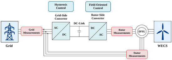
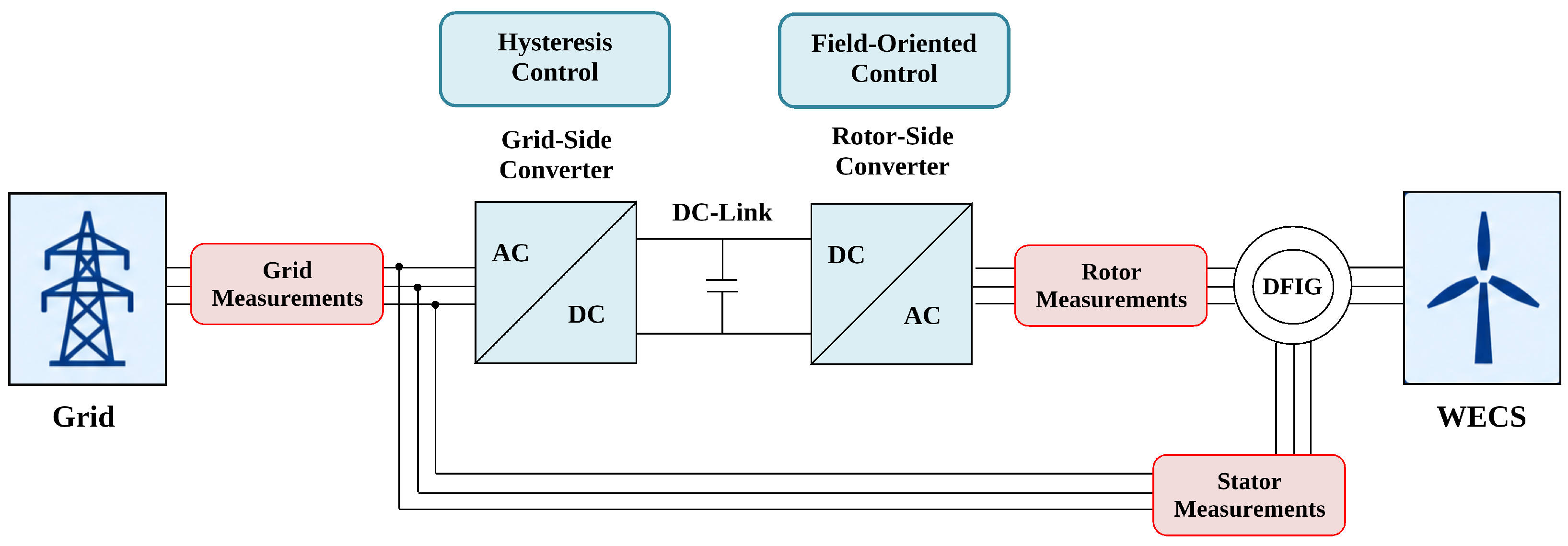
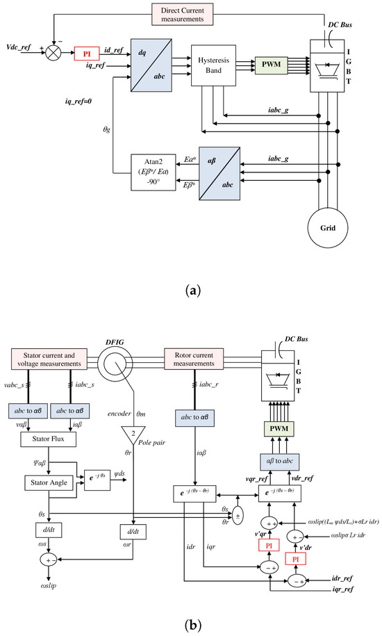
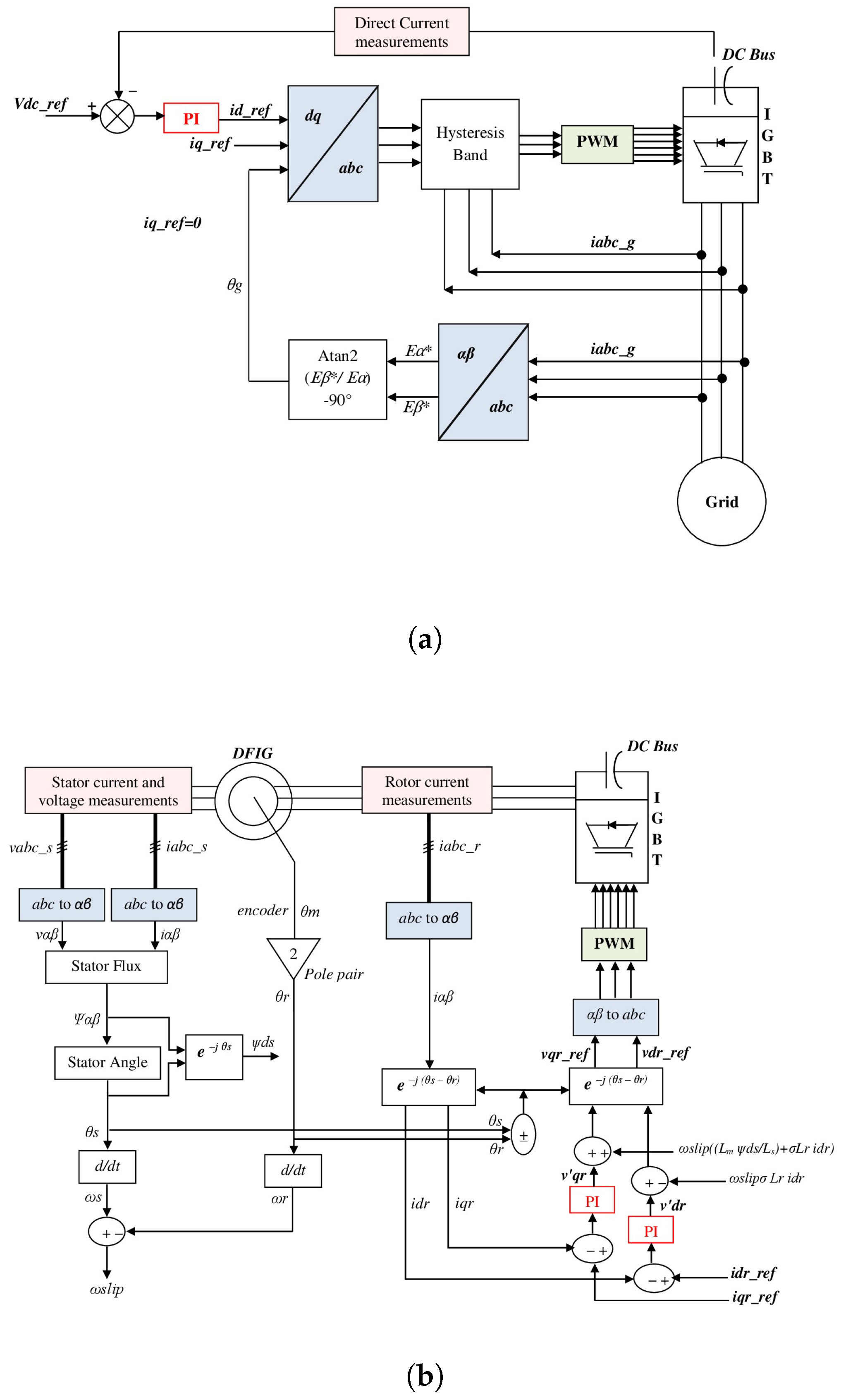
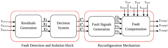
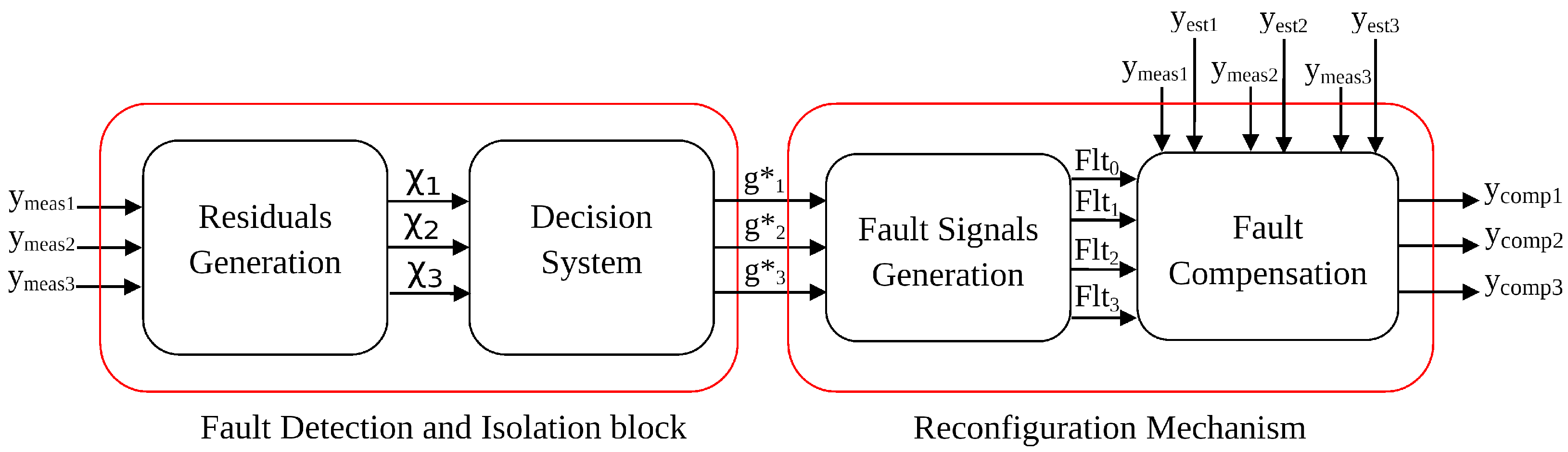


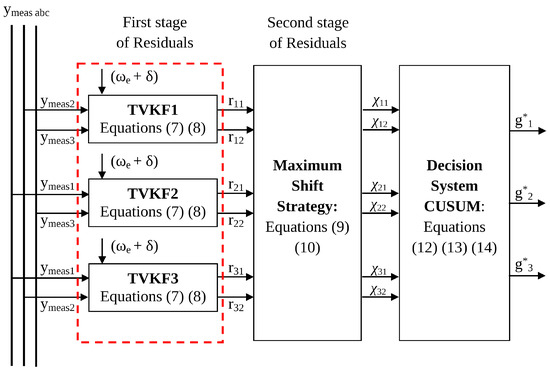
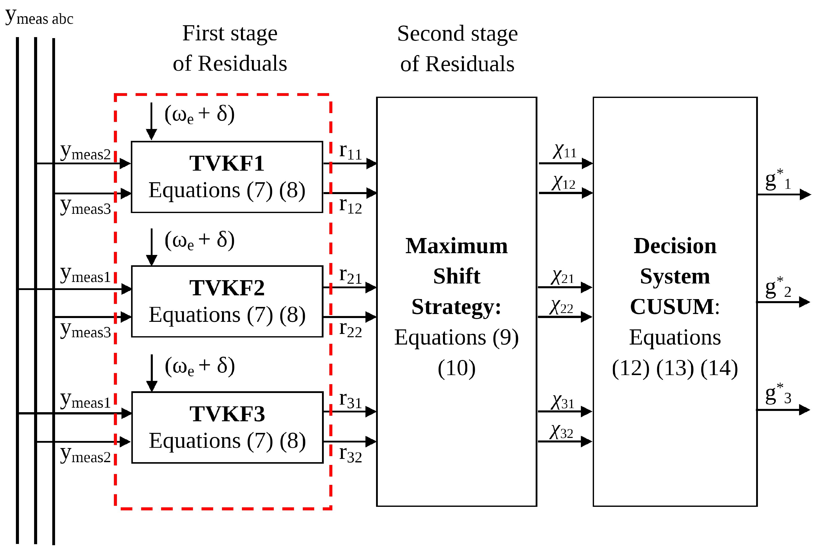
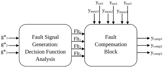
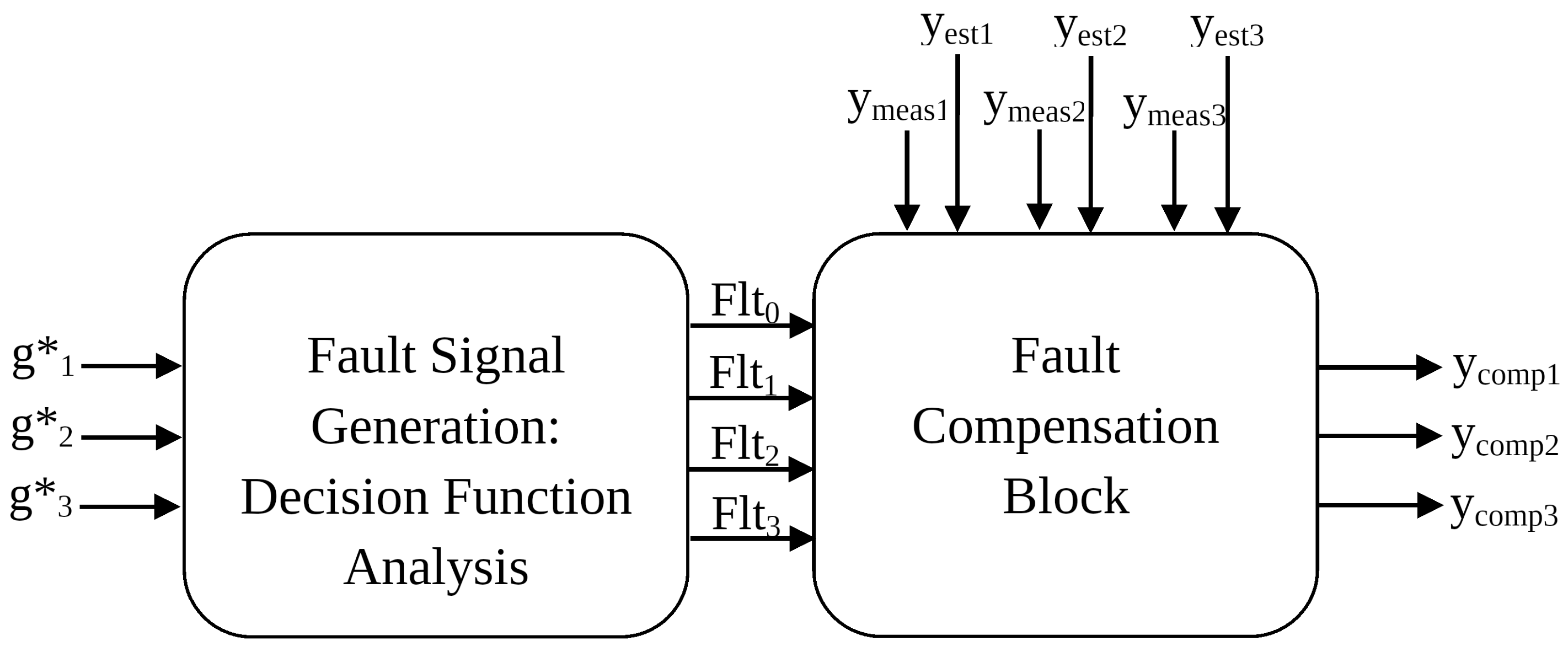
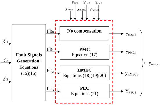
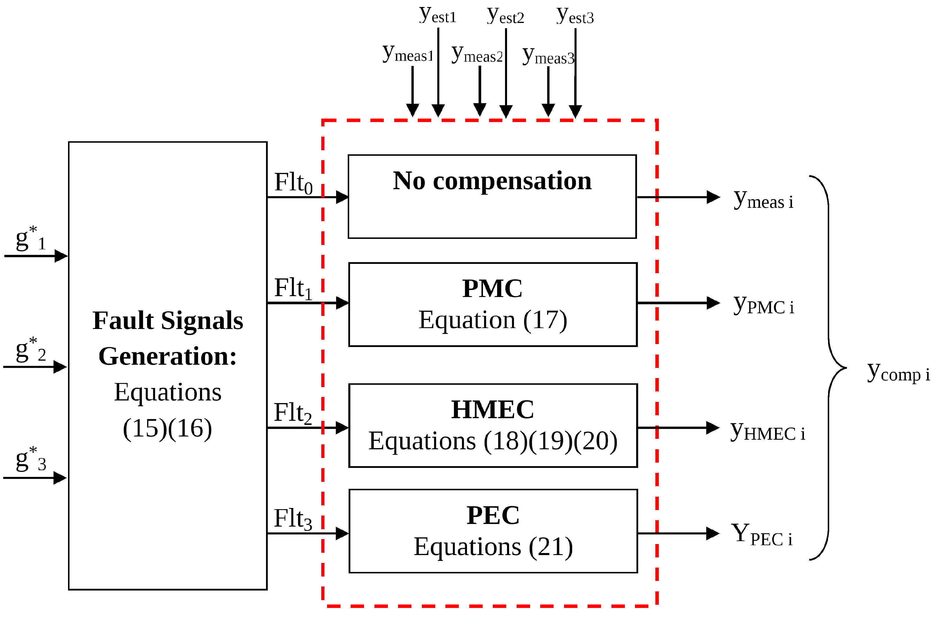
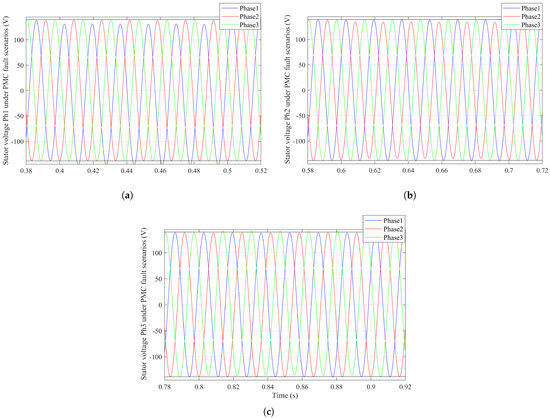
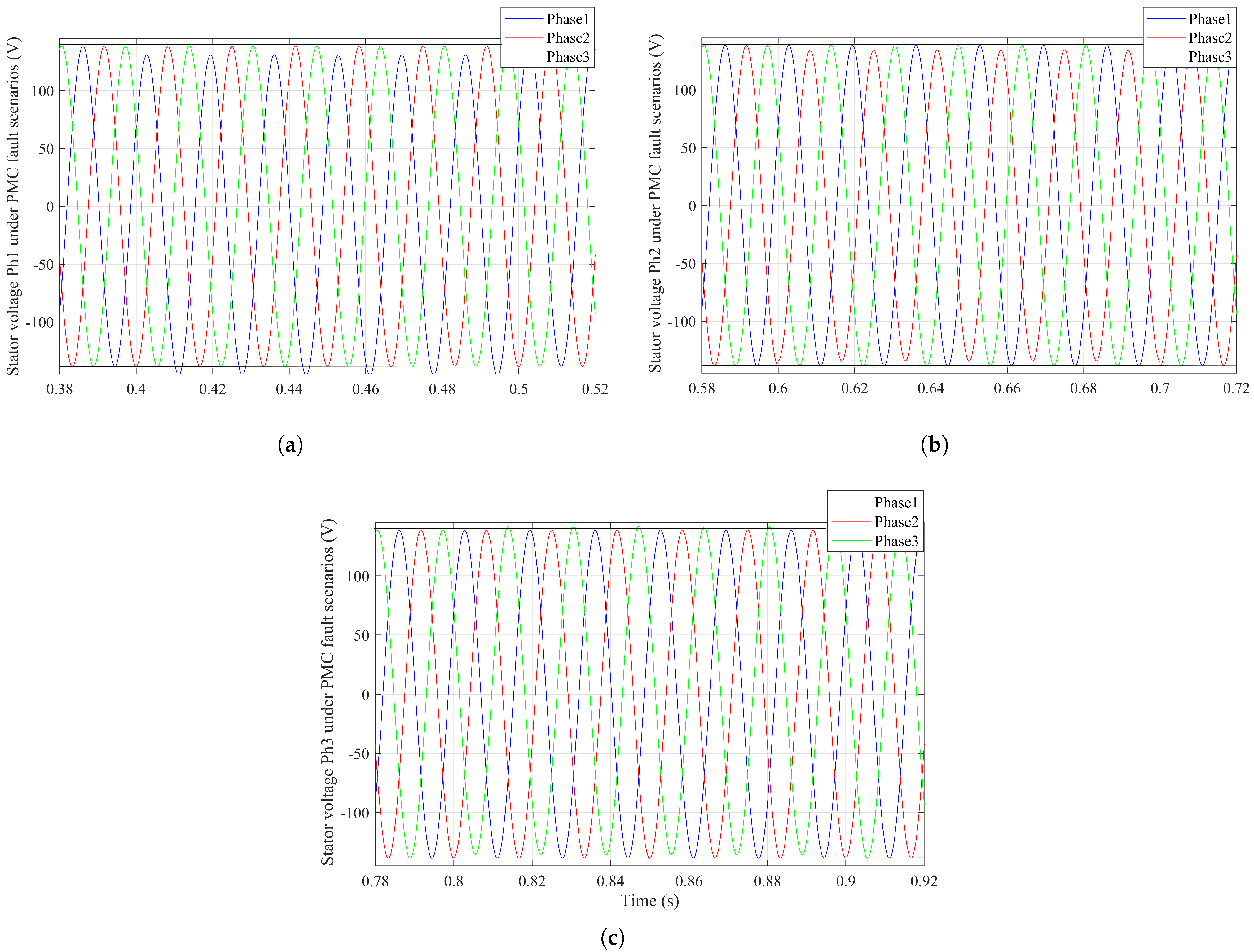
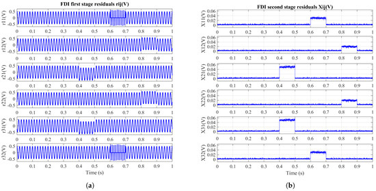
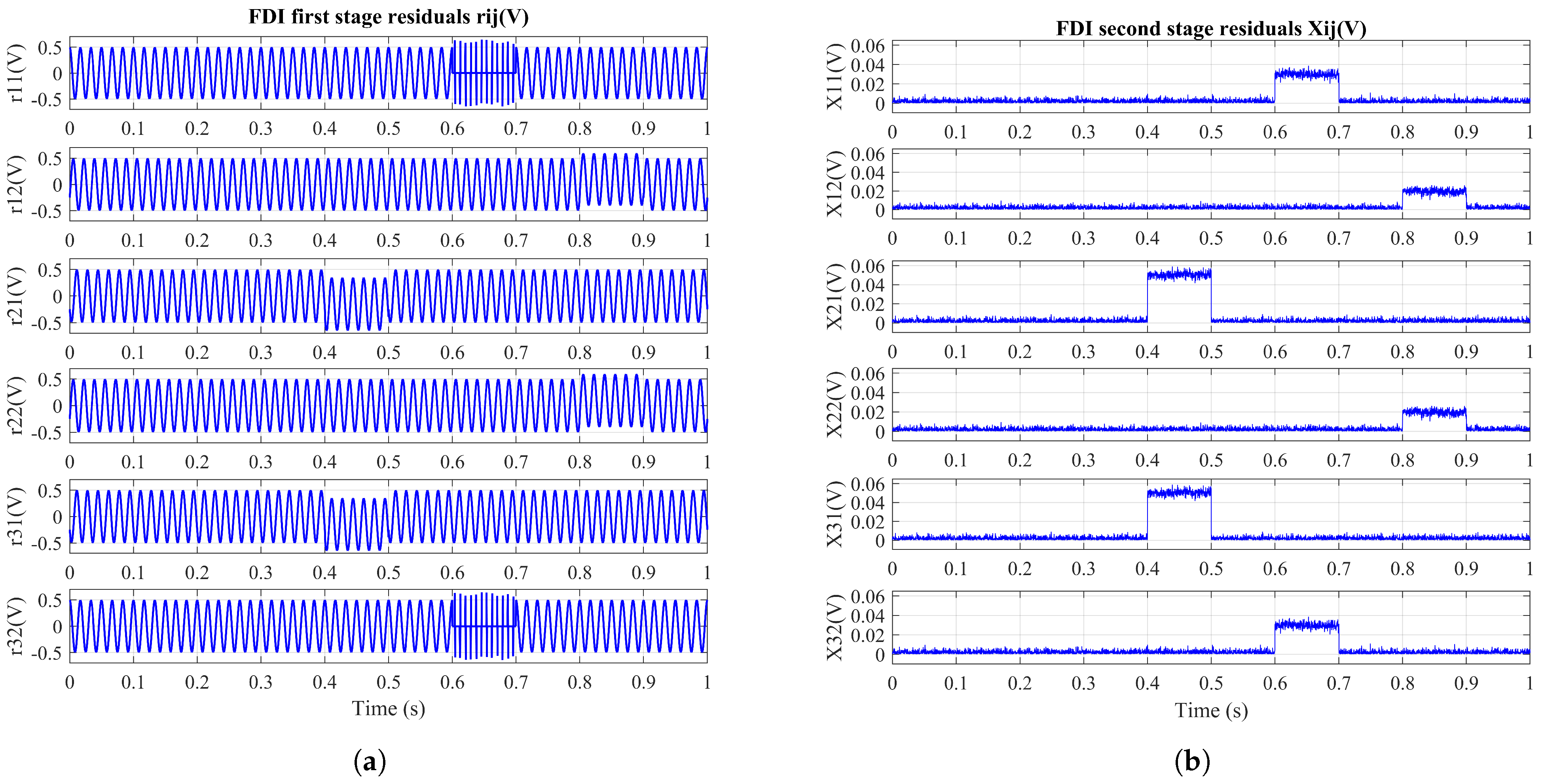
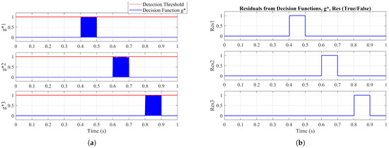
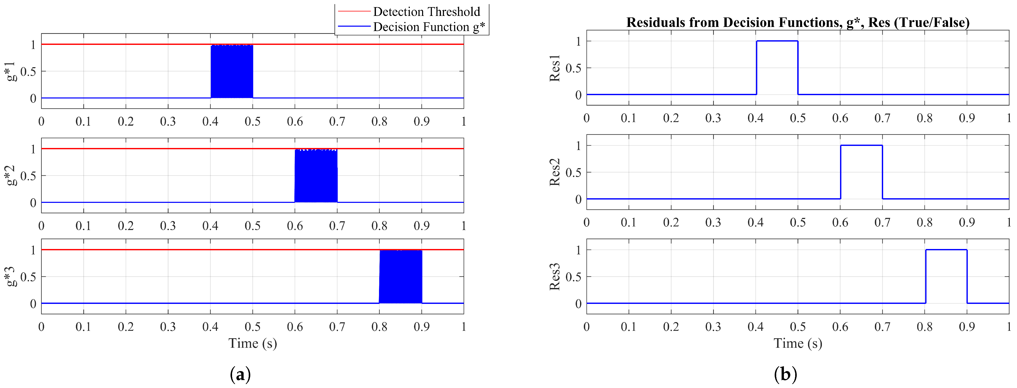
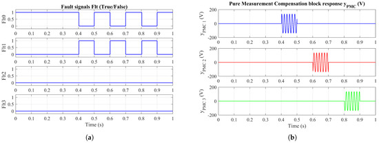
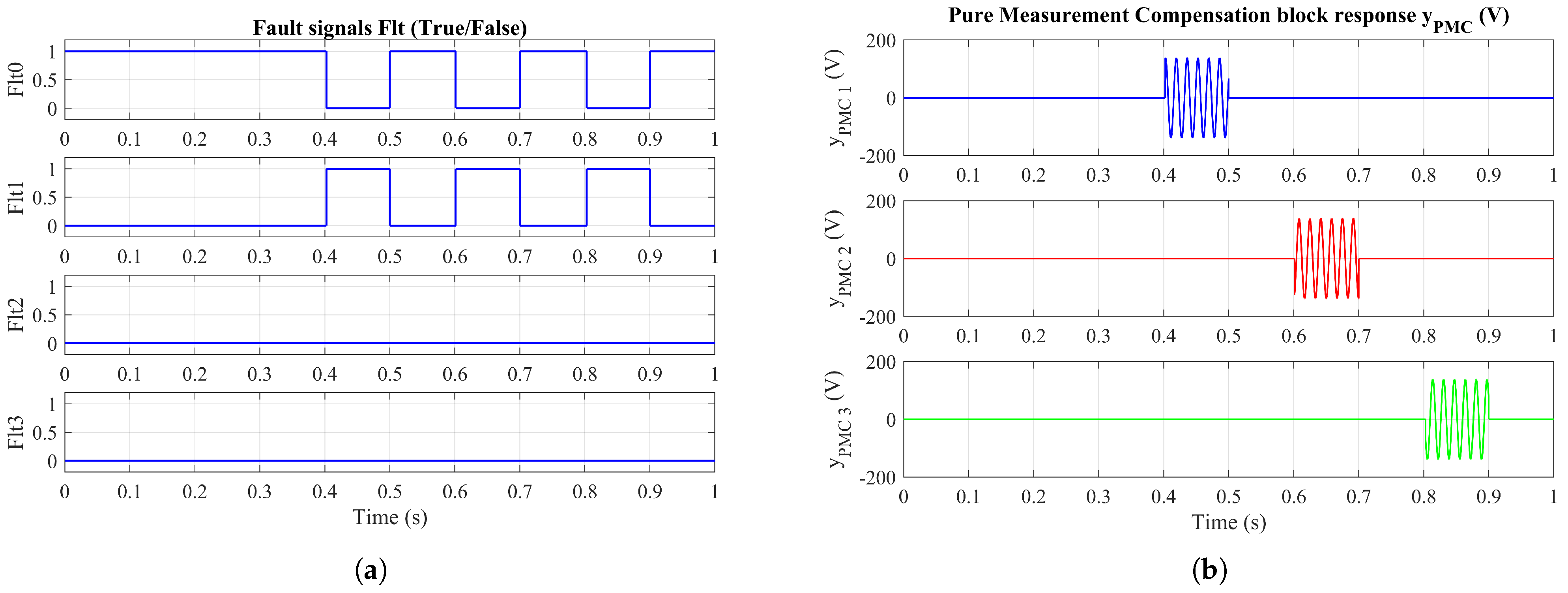
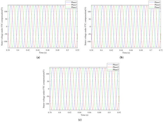
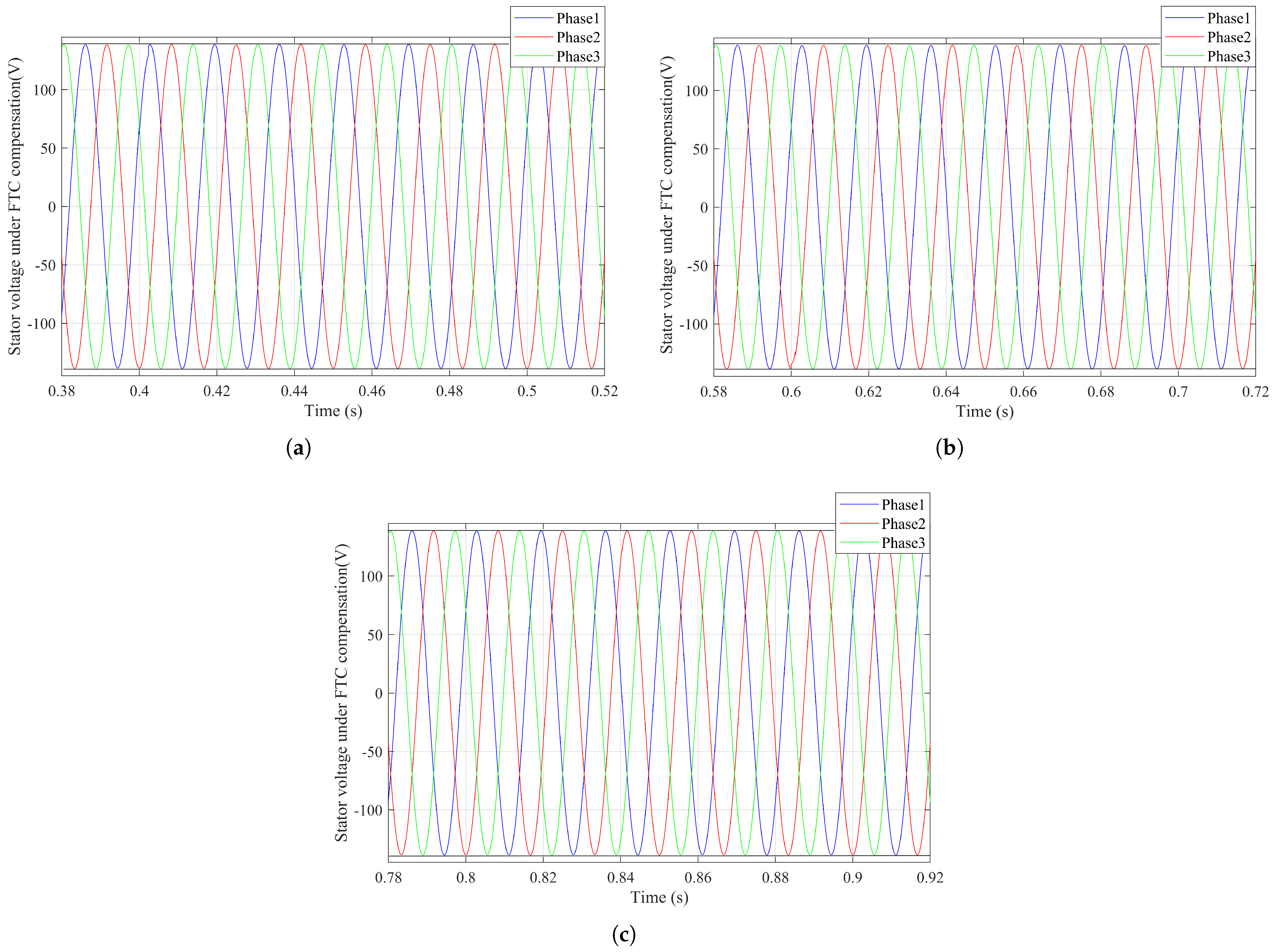
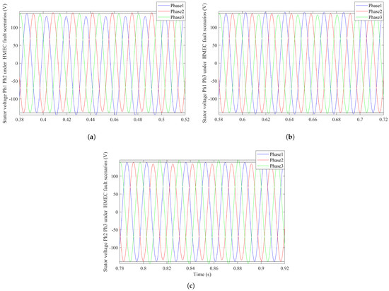
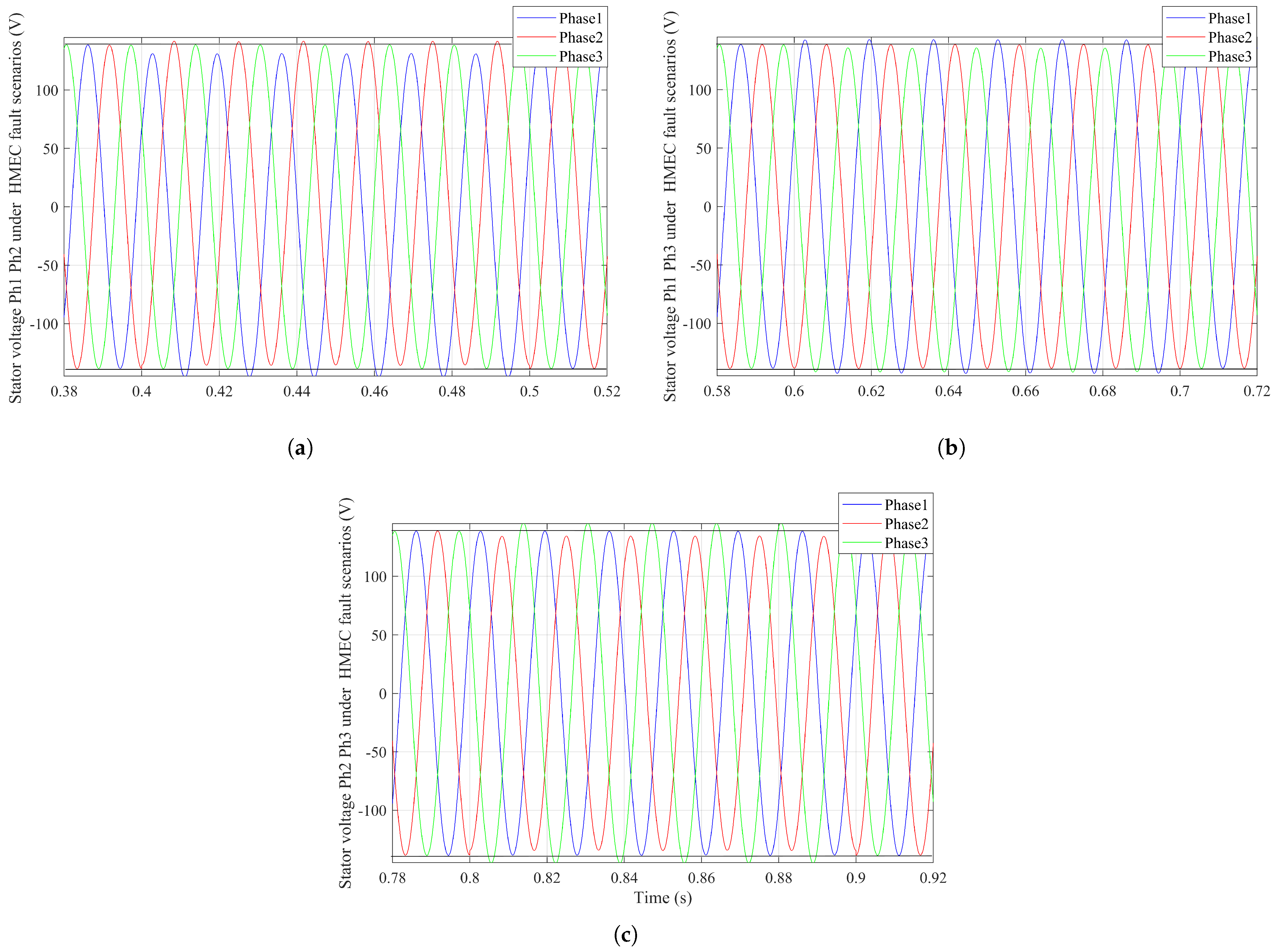
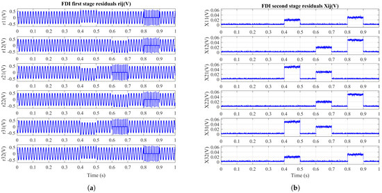
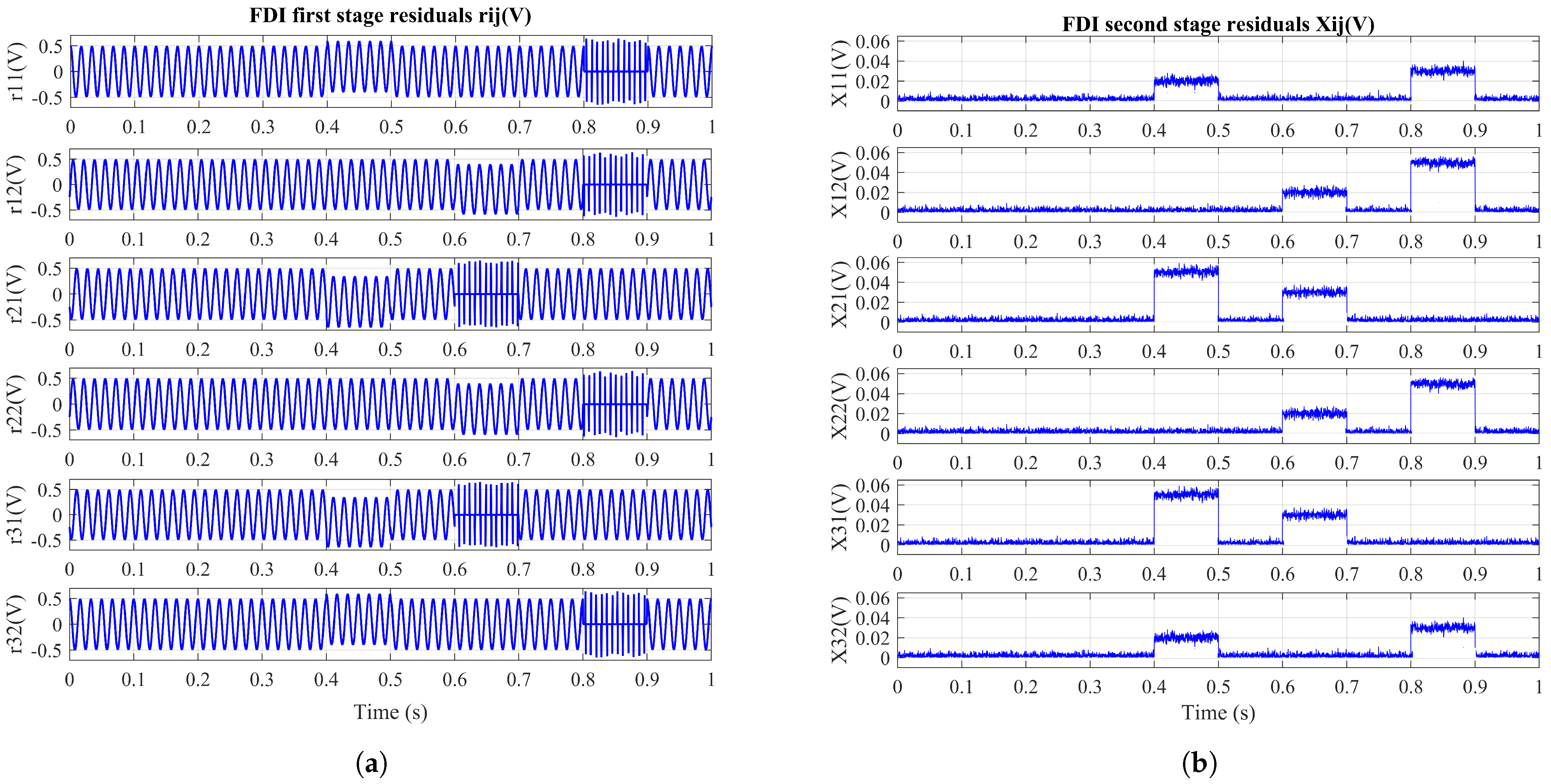
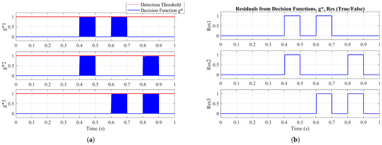
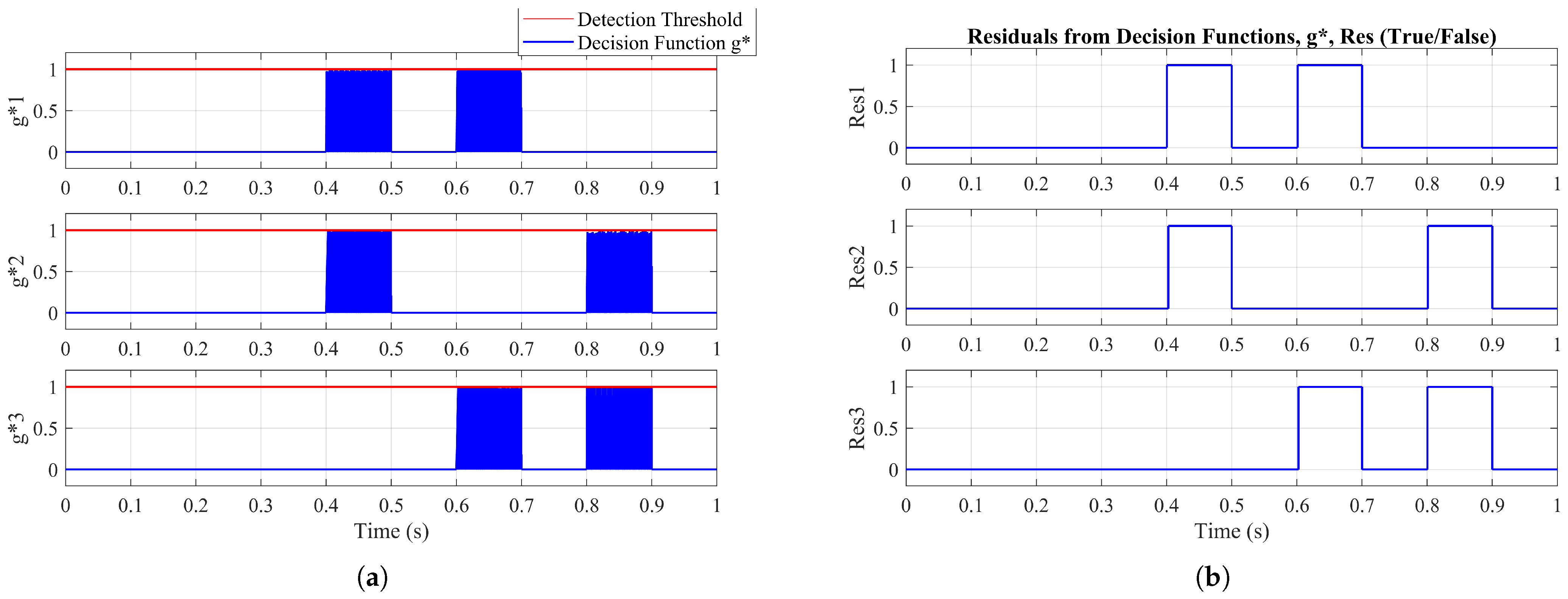
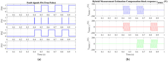
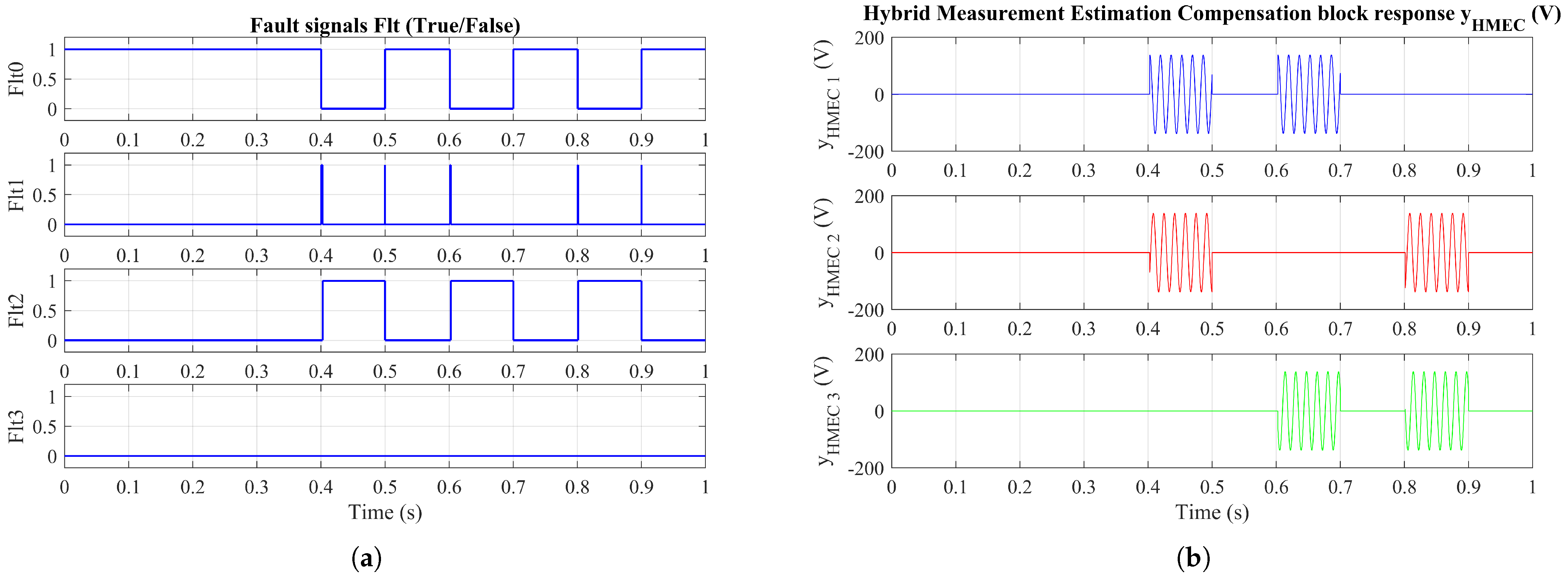
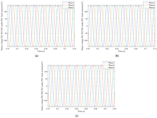
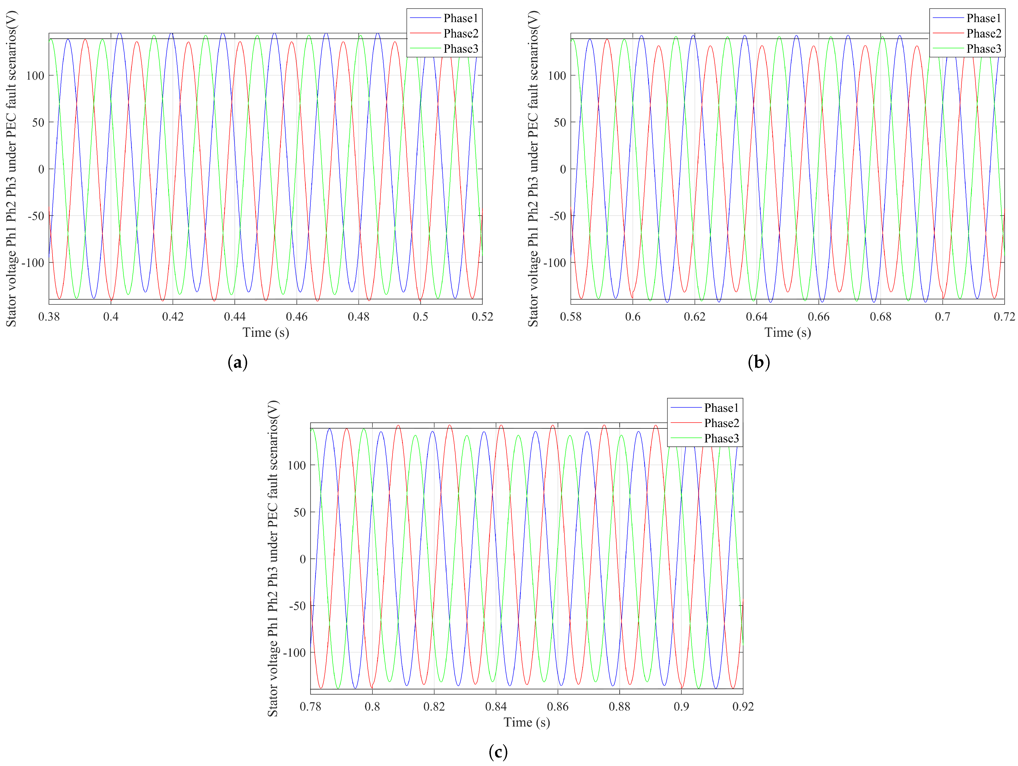
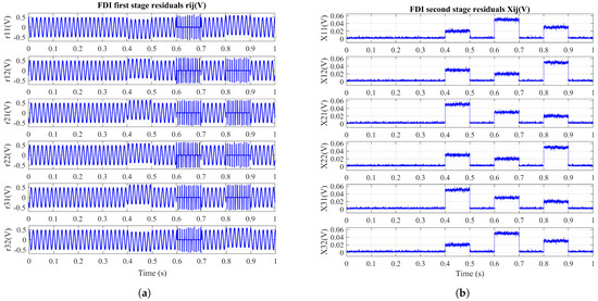
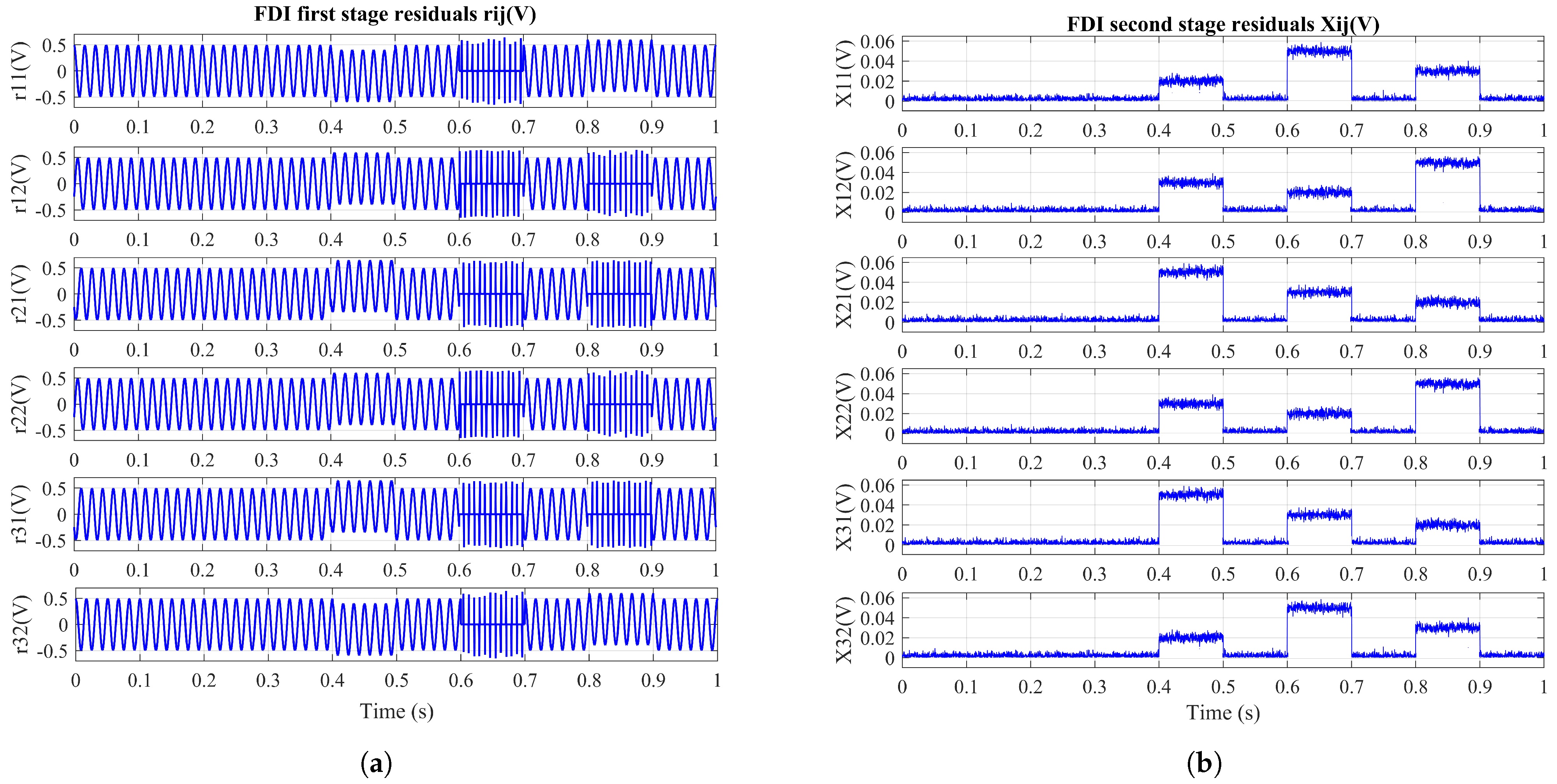
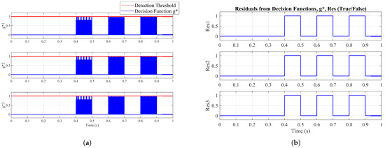
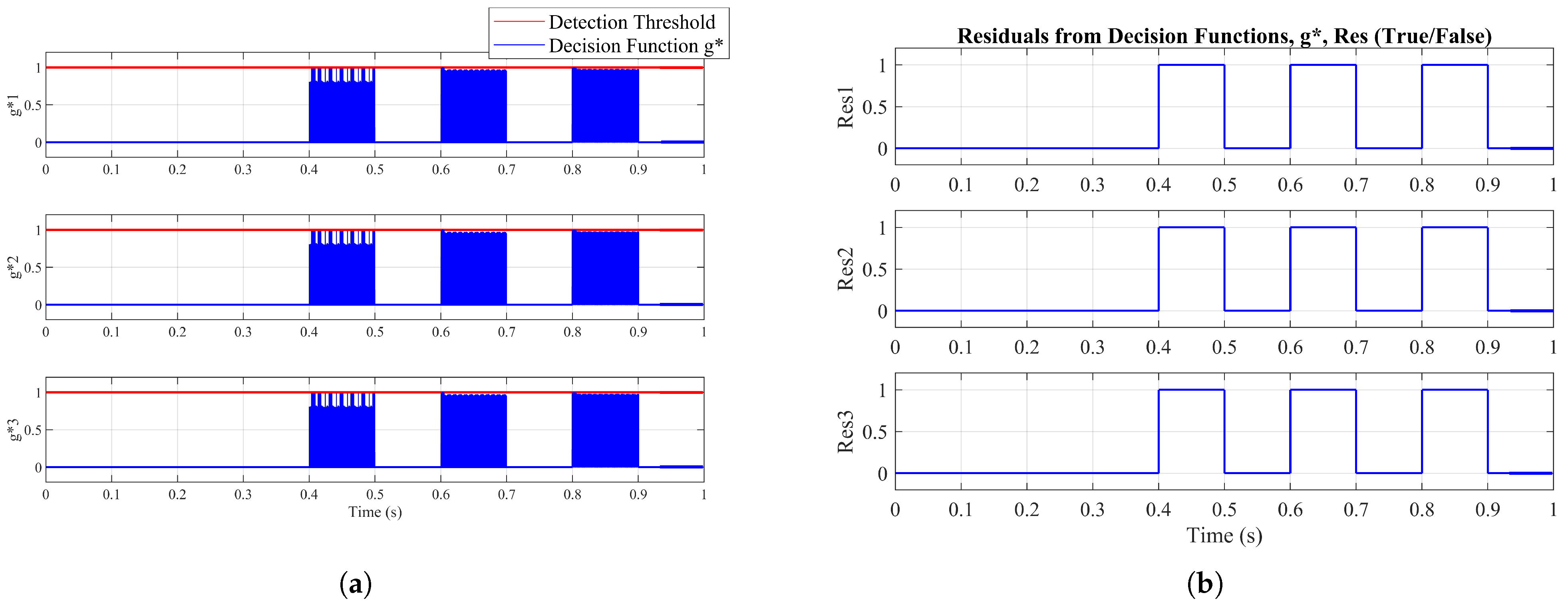
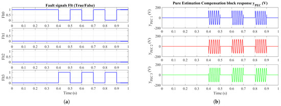
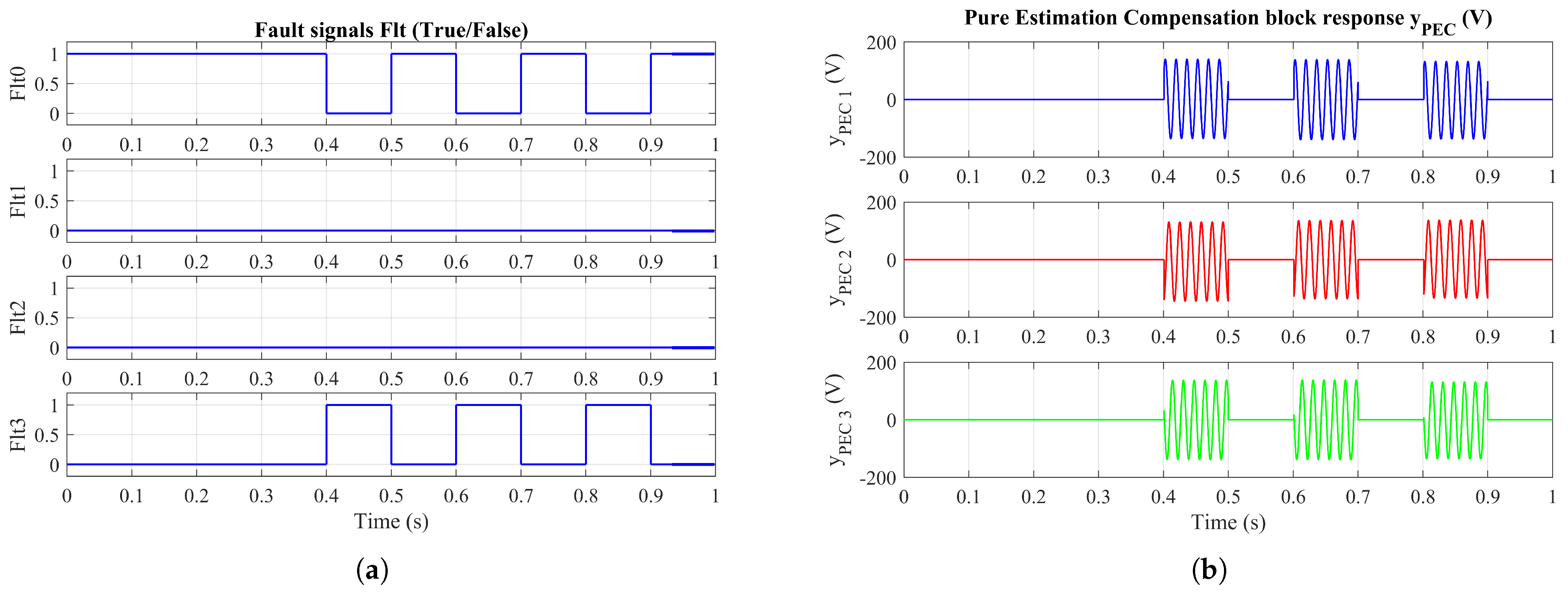
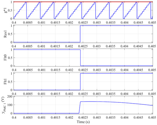
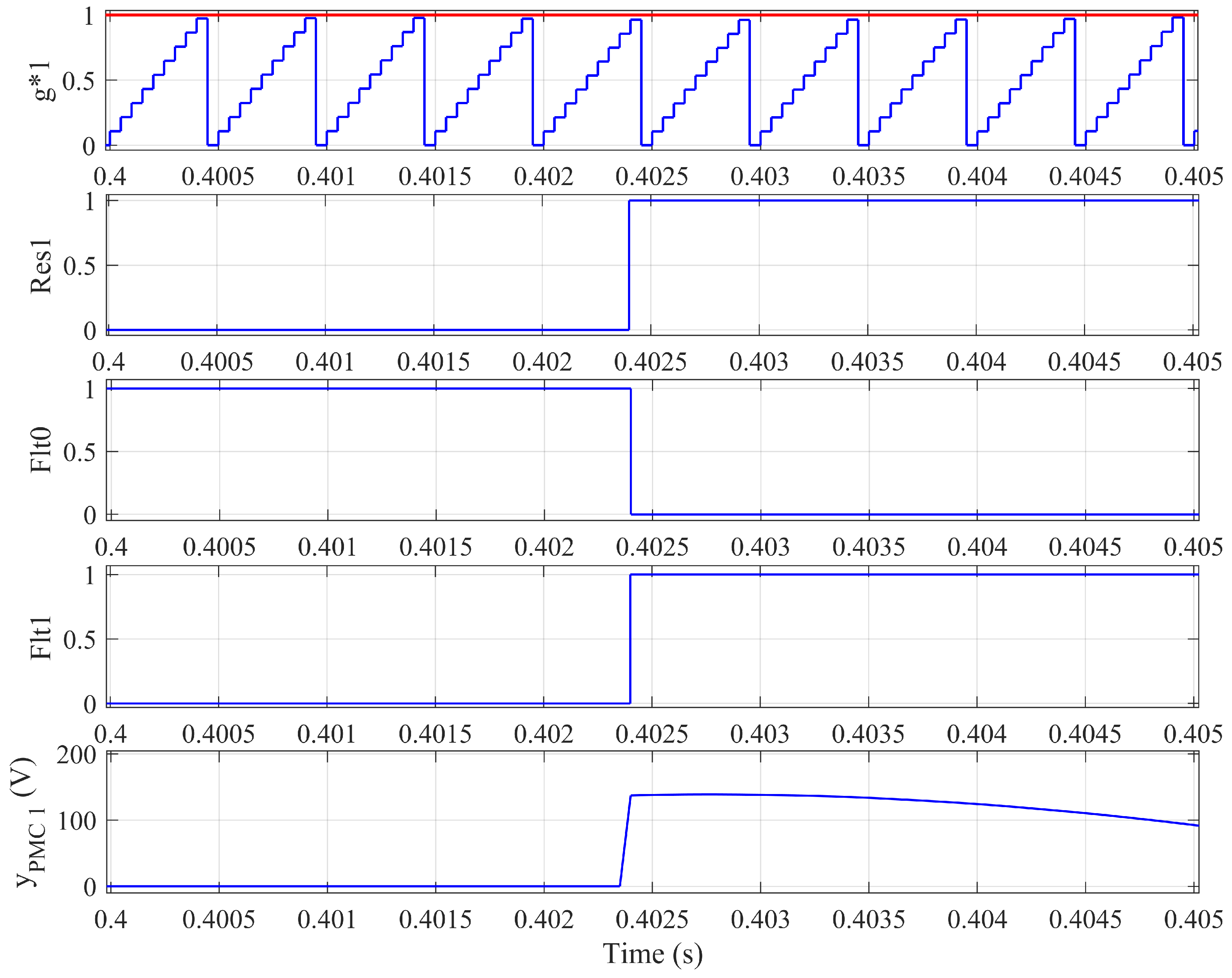
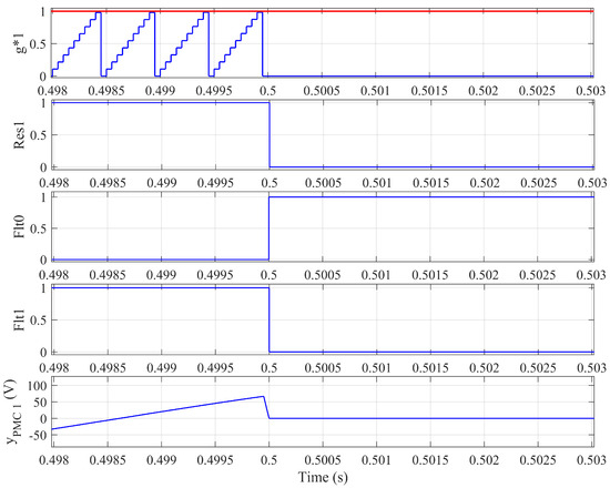
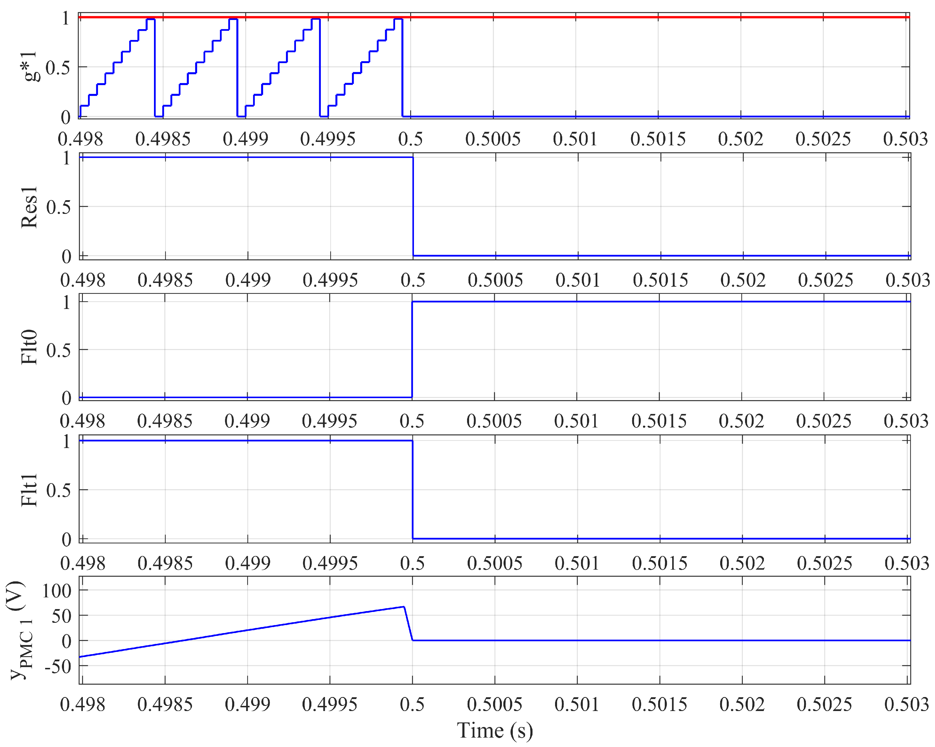

Disclaimer/Publisher’s Note: The statements, opinions and data contained in all publications are solely those of the individual author(s) and contributor(s) and not of MDPI and/or the editor(s). MDPI and/or the editor(s) disclaim responsibility for any injury to people or property resulting from any ideas, methods, instructions or products referred to in the content. |
© 2026 by the authors. Licensee MDPI, Basel, Switzerland. This article is an open access article distributed under the terms and conditions of the Creative Commons Attribution (CC BY) license.