


Abstract
This article presents an analysis and experimental verification of control strategies for a heat recovery system from air compressors operating under varying conditions. The research was conducted on three test benches equipped with compressors with rated powers of 30 kW, 75 kW and 110 . Based on experimental data, the dynamic properties of the system were identified using FOPDT models, demonstrating a significant dependence of the model parameters on the operating point. Subsequently, a comparative analysis of P, PI, and PID controllers and various methods for selecting their settings was conducted. Further studies included a PI controller with fixed settings, a gain–scheduling strategy, and adaptive control using online identification of model parameters by the RLS method. It was demonstrated that the variability of the system’s dynamic properties limits the applicability of a PI controller with fixed settings over the entire analyzed operating range. The application of adaptive control enabled continuous adjustment of controller settings to the changing properties of the plant without the need to determine models and settings for multiple operating points in advance, as required by the applied gain–scheduling strategy. In a selected experiment with the adaptive controller, stable water temperature control was achieved with heat exchanger heat balance indicator values exceeding 90%. This indicator defines the ratio of the heat flow rate absorbed by the water to the heat flow rate released by the oil and does not constitute a measure of the overall waste heat recovery efficiency of the compressor. The results confirm the feasibility of applying adaptive control for temperature regulation in heat recovery systems from compressors operating under varying conditions.
1. Introduction
Compressed air systems are widely used in industrial processes, among others, to drive pneumatic equipment, transport materials, automate processes, and carry out technological operations. Their widespread use, however, is associated with significant electricity consumption. The literature indicates that in selected industrial economies compressed air systems may account for approximately 10% of industrial electricity consumption [1,2,3]. For this reason, reducing the energy intensity of compressed air generation and use constitutes an important element of activities related to improving the energy efficiency of industrial plants. The energy efficiency of compressed air systems can be improved at various stages of compressed air generation, distribution, and use. The most frequently analyzed measures include reducing leakage, proper selection of compressors for the demand profile, and improving the management of the entire system [1,2,3,4,5,6]. One of the important directions is also the use of thermal energy generated during the compression process. Heat recovery from compressors is indicated both in the scientific literature and in recommendations concerning the improvement of the energy efficiency of industrial compressed air systems [2,7,8,9]. A significant part of the energy supplied to the compressor is ultimately dissipated in the form of heat. In the case of oil-injected screw compressors, a significant part of this energy is absorbed by the oil circuit and can be utilized outside the compressor by means of an additional heat exchanger. The literature indicates that energy recovered from compressors can be used, among others, for heating process water, preparing domestic hot water, or carrying out other processes requiring thermal energy [8,9]. Analyses of industrial heat recovery systems also confirm the possibility of obtaining significant energy and economic benefits through the utilization of waste heat from compressors [7,8,10]. Previous studies on compressed air systems focus largely on assessing their energy efficiency, identifying losses, optimizing the production and consumption of compressed air, and determining the potential for energy recovery [1,2,3,4,5,6,7]. In the case of heat recovery, the analyses primarily concern the available amount of energy, the configuration of the heat exchanger, and the possibility of practical utilization of the recovered energy [8,9,10]. From the point of view of industrial application, however, it is important not only to determine the maximum energy potential of the system, but also to maintain the required heat reception parameters under changing operating conditions. The heat exchange process between the compressor oil circuit and the water circuit is characterized by dynamics dependent on the current operating point. Changes in the temperatures of the media and the flow rate may cause changes in the static gain, time constant, and process delay. Similar properties are observed in other heat exchange systems, for which the application of a single linear model and a controller with fixed settings may lead to deterioration of control quality outside the operating point used during tuning [11,12,13,14,15]. This problem becomes particularly important in the case of a compressor heat recovery system, because thermal conditions may change both on the heat source side and on the heat receiver side. One way to account for the variability of process dynamics is to apply a gain–scheduling strategy, in which the controller settings are changed depending on the current operating point. Such an approach has been analyzed, among others, in the control of heat exchangers and other thermal processes [11,12,13,16]. Its application, however, requires determining the properties of the plant at an appropriate number of operating points and determining relationships that enable changes in the controller parameters. In the case of implementing the solution in different industrial configurations, this may increase the scope of identification and parameterization work required during system commissioning. An alternative is provided by adaptive strategies, in which information about the current dynamic properties of the process is obtained during its operation. Recursive parameter identification methods, including the recursive least squares (RLS) algorithm, enable the model to be updated based on successive process measurements and then the obtained parameters to be used to modify the controller settings. The possibility of using online identification and adaptive control in thermal processes has been demonstrated in the literature, particularly for plants whose properties change with operating conditions [17]. Such an approach is interesting from the point of view of an industrial heat recovery system because it may reduce the need for prior determination of multiple plant models for different operating points.
Based on the conducted literature review, it can be stated that the energy potential of heat recovery from industrial compressed air systems is well recognized, as are the possibilities of applying advanced control methods in heat exchange processes. However, the experimental evaluation of a compressor heat recovery system taking into account the variability of its dynamic properties over a wide range of operating conditions and linking control quality with the direct energy effect remains an important issue. Particularly important from the point of view of industrial application is the possibility of reducing the scope of prior multi-point identification and parameterization required during system commissioning. The aim of the work is the experimental analysis of the dynamic properties of a heat recovery system from air compressors operating under different conditions and the development and verification of a control strategy enabling water temperature stabilization while maintaining a high level of heat recovery. The research was conducted on three test stands equipped with compressors with powers of 30 kW, 75 kW and 110 .
The main contributions of the work can be summarized as follows:
- The variability of the dynamic properties of the heat recovery system was experimentally demonstrated over a wide range of operating points for compressors with powers of 30 kW, 75 kW and 110 ;
- An experimental comparison of control strategies was carried out, indicating the limitations of a PI controller with fixed settings and the practical limitations of the gain–scheduling strategy requiring prior multi-point parameterization;
- A strategy for adaptive adjustment of PI controller settings based on online identification of the plant model parameters was developed and verified;
- The assessment of temperature control performance was supplemented with an analysis of the heat exchanger heat balance, achieving heat balance indicator values of in a selected experiment with the adaptive controller.
The remainder of the article is organized as follows. First, the importance of heat recovery in compressed air systems was presented and the research problem was formulated. Next, the test stands were described and the dynamic properties of the system under different operating conditions were identified. Subsequently, a comparative analysis of the considered control strategies was presented and their impact on heat recovery efficiency was evaluated. The article was concluded with a discussion of the obtained results and a presentation of the most important conclusions.
2. Significance of Heat Recovery in Compressed Air Systems
The air compression process is a highly energy-intensive process. In practice, a significant part of the electrical energy consumed by the compressor is ultimately converted into thermal energy, while only part of it remains associated with the energy of the compressed air. Modern screw compressors are characterized by high mechanical efficiency; however, the energy associated with mechanical losses is also ultimately converted into heat. As a result, the compressor can be treated not only as a consumer of electrical energy, but also as a potential source of thermal energy that can be further utilized. Depending on the design of the device and its operating conditions, a significant part of the energy supplied to the compressor can be recovered in the form of useful heat. The recovered thermal energy can be used for space heating, domestic hot water preparation, or for technological processes. Heat recovery from both compressed air and oil is technically possible. In practice, however, a large part of the thermal energy generated during compression is absorbed by the cooling and lubricating oil. From the user’s point of view, it is important that the oil circuit provides the possibility of recovering a large amount of heat with a relatively simple design of the heat recovery system. This means that the heat accumulated in the oil can be effectively transferred to the receiving medium and further utilized. Therefore, the presented research focused on heat recovery from the compressor oil circuit. This solution makes it possible to utilize a large part of the heat generated during compressor operation and increase the energy efficiency of the entire system. In such a case, the water temperature at the outlet of the heat exchanger can be used as the controlled variable, while the flow rate of the heat-receiving medium can be used as the manipulated variable. A change in the medium flow rate affects the amount of heat removed from the oil, and thus the temperature of the water leaving the heat exchanger. The control method defined in this way makes it possible to continuously adjust the intensity of heat removal to the current operating conditions of the system. The water temperature at the outlet of the heat exchanger provides feedback information for the controller, on the basis of which the flow rate of the receiving medium is corrected. In practice, the primary objective of the system is not only to maximize the amount of recovered energy, but also to ensure safe operating conditions for the compressor. Excessive heat removal may lead to an excessive reduction in oil temperature, an increased risk of moisture condensation, and deterioration of lubrication conditions. On the other hand, insufficient heat removal may result in overheating of the compressor. Therefore, oil temperature is an important parameter associated with the safe operation of the screw unit, bearing durability, lubrication conditions, and stable operation of the device. Heat recovery should therefore be carried out while simultaneously maintaining the oil temperature within the required range, bounded from below and above by limit values. These values constitute overriding criteria for the control system. When the oil temperature approaches the limit values, the system should reduce the intensity of heat recovery or temporarily switch it off, regardless of the current heat demand on the receiving side. This means that the safe operation of the compressor has overriding priority over energy efficiency and the amount of recovered heat. The issue of supervisory control of compressor operating safety, including, among others, limiting or temporarily switching off heat recovery depending on the oil temperature, is beyond the scope of this article. Due to the complexity of the entire issue and the wide range of possible operating states of the system, the analysis was limited to one of its areas, i.e., controlling the water temperature at the outlet of the heat exchanger by regulating its flow rate. The issue of supervisory constraints, safety conditions, and mutual relationships between the individual control levels constitutes a separate problem. For this reason, the remainder of the article focuses on the selected control problem.
3. Problem Formulation
Based on the information presented so far, the following research problem was formulated:
Research problem: How to ensure stable control of the water temperature in a compressor heat recovery system under changing dynamic properties of the plant, while simultaneously maintaining a high level of recovery of the available thermal energy? In order to solve the formulated problem, a comparative analysis of selected control strategies was carried out in the further part of the article, including P, PI and PID controllers, a controller with variable parameters, and an adaptive control system.
The main contribution of the work includes:
- Experimental identification of the dynamic properties of the heat recovery system at different operating points;
- Comparison of control quality indices for selected control strategies;
- Experimental verification for three physical air compression systems with powers of 30 kW, 75 kW and 110 .
4. Experimental Test Benches
In order to conduct research related to the formulated problem, three test stands with oil–water heat exchangers were designed and constructed, intended to operate with compressors with rated powers of 30 kW, 75 kW and 110 (Figure 1). Each test stand was incorporated into the oil circuit of the corresponding compressor. The use of compressors with different powers made it possible to conduct research on systems with different parameters and operating conditions. Before constructing the test stands, the requirements relevant from the point of view of the planned research were analyzed. The most universal possible assumptions were adopted, corresponding to the operating conditions of compressors in an industrial environment, with particular emphasis on their operational requirements.
Figure 1.
Test stands with oil–water heat exchangers, intended to operate with compressors with rated powers of 30 (a), 75 (b), and 110 (c).
Each test stand consisted of:
- Endress+Hauser Promass 300 flow meter, providing direct measurement of the oil mass flow rate with a maximum measurement error of .
- Aplisens APR-2000ALW differential pressure transmitters, providing direct measurement of the oil pressure drop on the test benches, with a maximum measurement error of .
- Class A PT100 TiTEC KBTF/PT100/2.0/S/4L temperature sensors (4 units), connected in a 3-wire configuration to PT100 SBW transmitters with a 4 to 20 output, providing temperature measurement with a maximum measurement error of at and at for measuring the oil supply and return temperatures and the water supply and return temperatures.
- Oil–water heat exchanger.
To ensure repeatable conditions for conducting the research, a separate cooling water preparation and distribution stand was also designed, operating with all three oil–water heat exchanger stands (Figure 2). This system enabled the test stand to be brought to a steady state after completion of the test of a given control strategy. This made it possible to start subsequent tests under comparable initial conditions, which was particularly important in the comparative analysis of control strategies and the results obtained for compressors with different powers.
Figure 2.
Cooling water preparation and distribution stand (indoor unit).
The cooling water preparation and distribution stand was constructed in the form of an external cooling system (Figure 3). It consisted of:
Figure 3.
Cooling water preparation and distribution stand (outdoor unit).
- IFM SM electromagnetic flow meters (SM7000, SM8000, SM8020), providing direct measurement of the volumetric flow rate, with a maximum measurement error of .
- PT100 temperature sensor (in a configuration analogous to that used on the heat exchanger test benches), used in the cooling water temperature control system.
- Three Grundfos Magna 3 32-120-180 pumps, operating in “constant curve” mode and controlled by an analog 4 to 20 signal to regulate the cooling water flow rate.
- Siemens VXF32.50-40 three-way valve with a SAX61.03 actuator, used to regulate the cooling water temperature.
For process data acquisition, the following equipment was used (Figure 4):
Figure 4.
Main elements of the measurement system (respectively: recorder (a), analyzers (b), control module (c), personnel station (d)).
- LAB-EL LB-490 digital data logger, equipped with four expansion modules, increasing the total number of measurement channels to 28, used to measure temperature, oil and water flow rates, pressure, and compressor phase current; analog 0 to 20 current inputs were used, providing a measurement accuracy of .
- Three Siemens SENTRON PAC3200 electrical energy analyzers, operating with J&D Electronics JS24S series current transformers, used mainly to measure instantaneous electrical power, with a maximum measurement error of for the 30 and 75 test benches and for the 110 test bench.
- PT100 temperature sensors (in a configuration analogous to that used on the heat exchanger test benches), intended to measure the ambient temperature around the compressors and the outdoor air temperature.
- Control module, using a Siemens S7-1200 PLC, equipped with digital and analog input and output modules.
- Operator station equipped with an HP EliteBook 8760w laptop computer and a Siemens SIMATIC PANEL KTP600 touch panel.
Dedicated software operating with the measurement equipment and control system was used to perform measurement tasks and to record, analyze, and visualize data:
- LAB-EL LBX software, used to operate the measurement system, control connected devices, and monitor and record measurement data. The software also enabled visualization of recorded data in the form of charts, reports, and histograms, as well as multi-workstation operation over a computer network.
- Advanced TCP/IP Data Logger software, supporting the acquisition of measurement data from electrical energy analyzers, used in its commercial version as an alternative to the dedicated software provided by the analyzer manufacturer.
- control software for the SIMATIC S7-1200 CPU 1212C controller, developed in the TIA Portal V14 environment, used to implement control algorithms, handle input and output signals, and communicate with the components of the control and measurement system.
The test benches, together with the cooling water preparation and distribution system and the control and measurement equipment, were installed in the compressor room of an industrial plant. This made it possible to conduct research under real industrial conditions. The prepared test benches enabled systematic experiments at defined operating points while maintaining conditions characteristic of actual industrial operation. Due to the experimental nature of the research, particular attention was paid to verifying the correctness of the readings from the temperature measurement channels. During the experiments, differences were observed between the readings of individual temperature sensors; therefore, their readings were periodically verified using an ice point reference. The sensors were placed in a mixture of water and ice at a reference temperature of approximately 0 , and individual offset corrections were introduced based on the observed differences in readings. This procedure was performed several times during the research, enabling periodic verification of the measurement channels and reducing the influence of differences in sensor readings on the recorded temperature values. The applied procedure constituted a practical, single-point verification of sensor readings and was not a complete multipoint laboratory calibration. Within the presented research, no separate metrological analysis of the complete measurement system or formal analysis of measurement uncertainty propagation was conducted. This should be considered one of the limitations of the experimental research.
In the first stage of the research, the dynamic properties of the system were identified at different operating points. The objective of the identification was to determine the influence of operating conditions on the dynamics of the plant and to identify properties relevant to the selection of a control strategy. The identification procedure and the obtained results are presented in the following section.
5. System Identification Under Different Operating Conditions
The investigated heat recovery system can be described using dynamic equations taking into account the heat exchange process and the properties of the individual system components. Such a description allows for a detailed representation of the system behavior; however, its direct use for the design and implementation of control algorithms under industrial conditions is difficult. Therefore, in the case of thermal systems, simplified models are often used, which, while preserving the most important dynamic properties of the plant, make it possible to reduce the complexity of its description. In this work, a First-Order Plus Dead Time (FOPDT) model was adopted as a compromise between the accuracy of representing the dynamics of the investigated process and the simplicity of the model required from the point of view of the design and implementation of the control system. A model of this type makes it possible to describe the basic dynamic properties of thermal processes, in particular their inertia, gain, and delay. At the same time, the small number of model parameters makes it possible to determine them based on measurement data for different operating points of the system. The adoption of a common model structure for the analyzed operating points additionally makes it possible to assess changes in the dynamic properties of the plant and provides a basis for the design and comparison of the control strategies considered in the work. The use of a simplified model was also important from the point of view of the subsequent implementation of the control system. Models used at the simulation research stage require the numerical solution of differential equations, which significantly complicates their direct application in a PLC controller. For this reason, the dynamics of the investigated system were described using a transfer function
where denotes the time constant, k—the static gain, and —the delay.
The adoption of the FOPDT model is also justified by the nature of the responses obtained on the test stands. An example response of the system to a step change in flow rate is shown in Figure 5. The observed response exhibits features characteristic of an inertial plant with delay, which justifies the use of the adopted model structure.
Figure 5.
Example response of the temperature at the heat exchanger outlet to a step change in flow rate for the test stand with a 75 compressor.
The water flow rate through the heat exchanger was adopted as the input signal during identification, while the water temperature at the heat exchanger outlet was adopted as the output signal. The oil temperature was simultaneously monitored as a parameter limiting the heat removal process in order to prevent excessive cooling of the oil. For each of the analyzed operating points, a step change in the input signal was performed and the system response was recorded. Based on the obtained responses, the FOPDT model parameters were determined. The identification procedure was implemented in Scilab using a least–squares criterion. The parameters k, , and were determined by minimizing the sum of squared differences between the measured heat exchanger outlet water temperature and the corresponding response of the FOPDT model:
where denotes the measured heat exchanger outlet water temperature, denotes the corresponding temperature predicted by the FOPDT model, and N is the number of samples used in the identification. The minimization procedure was performed independently for each analyzed operating point. The conducted identification made it possible to determine how the dynamic properties of the investigated system change depending on the operating point. The identification results for the 30 kW, 75 kW and 110 test stands are presented in Table 1, Table 2 and Table 3, respectively.
Table 1.
FOPDT model identification results for the test stand with the 30 compressor.
Table 2.
FOPDT model identification results for the test stand with the 75 compressor.
Table 3.
FOPDT model identification results for the test stand with the 110 compressor.
The obtained results indicate that the dynamic properties of the heat recovery system depend on the operating point. For all three test stands, changes in the values of the time constant and the delay were observed with changes in the water temperature at the heat exchanger inlet and the pump control signal. This means that the system dynamics change within the analyzed range of operating conditions. The ranges of changes in the determined model parameters for the individual test stands were:
- 30 test stand: –43 s, –15 s;
- 75 test stand: –118 s, –31 s;
- 110 test stand: –61 s, –23 s.
The presented ranges show that a change in the operating point may lead to significant changes in the dynamics of the investigated system. This is particularly evident for the 75 test stand, for which the determined time constant varied from 21 to 118 s, and the delay from 1 to 31 s. From the control point of view, this means that controller parameters selected for one operating point do not necessarily provide comparable control quality at the remaining operating points. The obtained identification results therefore provide the basis for conducting a comparative analysis of selected control strategies, presented in the next section.
Remark 1.
The adopted static gain value of was a modeling assumption and was not a direct result of the identification procedure. The identification showed that the actual gain value depended on the operating point and the adopted scale of the pump control signal. For example, at one of the operating points, the values , s, and s were obtained. The negative sign of the gain resulted from the inverse relationship between the pump control signal and temperature and was taken into account in the operation of the controller. Adopting was intended to simplify and standardize the procedure for determining controller settings while preserving the identified dynamic parameters τ and θ. It should be noted that directly using the small values of k obtained during identification led, according to the applied tuning relationships, to the determination of significantly higher proportional gain values . For example, for , the effect of the absolute value of the static gain alone on the scale of the calculated , compared with the case of , corresponds to a factor of . Furthermore, the numerical value of the parameter k was related to the scale of the control signal used during identification. Preliminary tests of P, PI, and PID controllers conducted using the PLC demonstrated the high sensitivity of the real system to the proportional gain value. For values greater than approximately 2.5, a rapid increase in the control signal to its maximum value was observed, and temperature oscillations also occurred during the tests. Consequently, the settings obtained directly from the complete identified model would require additional consideration of signal scaling and the structure of the controller implemented in the PLC before their direct application to the real system. For this reason, was adopted at this stage of the research, focusing the tuning procedure on changes in the dynamic properties of the process described by τ and θ. The settings determined in this way were subsequently verified experimentally on the real plant. From the perspective of the analyzed process, the primary evaluation criteria were the steady-state control error and the absence of undesirable temperature oscillations, whereas minimizing the settling time was not the overriding criterion.
Remark 2.
The identification studies were conducted manually on three test benches equipped with compressors with rated powers of 30 kW, 75 kW and 110 . For each compressor, four water temperature conditions and four pump control signal levels were considered: 25, 50, 75, and 100%, corresponding to a total of 48 operating points. The studies were spread over time and conducted under real operating conditions. Consequently, it was not possible to maintain identical thermal conditions during individual experiments. In particular, the air temperature inside the room housing the compressors and the outdoor air temperature varied during the research. For this reason, the observed variability of the identified FOPDT model parameters, including the delay θ, should not be interpreted directly as a measure of experimental uncertainty or repeatability under identical conditions. Individual parameter values correspond to different operating points and experiments conducted under changing thermal conditions. Repeating all experiments under exactly the same conditions was not possible because the ambient conditions were not independently stabilized. The obtained variability of the FOPDT model parameters therefore reflects changes in the dynamic properties of the real system over the analyzed operating range and provides additional justification for applying control strategies that enable the controller to adapt to changing process properties.
6. Comparative Analysis of Control Strategies
Based on the identification results presented in the previous section, a comparative analysis of selected control strategies was carried out. The research included classical P, PI and PID controllers, a controller with variable parameters, and adaptive control. The individual strategies were tested on three test stands with compressors with powers of 30 kW, 75 kW and 110 . The aim of the analysis was to compare the properties of the individual control strategies under variable operating conditions of the investigated system and to determine their suitability for controlling the heat recovery process. The following subsections present the method of selecting the parameters of the individual controllers, the procedure of the conducted research, and the obtained results.
Remark 3.
The presented time responses are selected examples from a broader range of conducted studies. A direct comparative analysis of individual control strategies was performed under operating conditions that were as similar as possible in order to limit the influence of differences in operating points on the obtained results and ensure the comparability of the analyzed strategies. At the same time, the adopted test scenarios covered a wide range of system operating points. A typical scenario included chiller cooling temperature setpoints of 20 °C, 30 °C, 40 °C, 45 °C and 50 . For each of these values, tests were conducted for six water temperature setpoints at the heat exchanger outlet, as shown in Table 4. The scope of testing for a given control strategy was extended to additional operating points if the obtained results indicated satisfactory stabilization of the water temperature at the heat exchanger outlet and the absence of undesirable oscillations. For this reason, not all analyzed controller configurations were tested over the entire presented range.
Table 4.
Typical operating points considered in the experimental test scenarios.
6.1. P, PI and PID Controllers
In the first stage of the analysis, classical P, PI and PID controllers were considered. The selection of their parameters required the adoption of one reference model for each test stand. Due to the variability of the model parameters depending on the operating point demonstrated in the previous section, a model with parameters determined on the basis of the mean values of k, and obtained for all analyzed operating points of a given test stand was adopted as the reference model. This approach made it possible to determine one set of model parameters for each test stand and to apply the same reference conditions during the selection and comparison of P, PI and PID controllers. Averaging the parameters does not imply the assumption of constant dynamic properties of the plant, but constitutes a reference point for the evaluation of classical controllers with fixed parameters. As a result of the averaging, the following model parameters were obtained:
- 30 test stand: s, , s;
- 75 test stand: s, , s;
- 110 test stand: s, , s.
Based on the determined models, the parameters of the P, PI and PID controllers were selected [18,19,20]. In order to compare different methods of selecting the settings, several tuning methods were applied for each controller type. For the P controller, three methods were used: Ziegler–Nichols (ZN), Chien–Hrones–Reswick (CHR), and Cohen–Coon (CC). For the PI controller, six methods were applied: Ziegler–Nichols (ZN), Chien–Hrones–Reswick (CHR), Cohen–Coon (CC), Approximate M-constrained Integral Gain Optimization (AMIGO), Internal Model Control (IMC), and Skogestad Internal Model Control (SIMC). For the PID controller, six methods were used: Ziegler–Nichols (ZN), Chien–Hrones–Reswick (CHR), Cohen–Coon (CC), Internal Model Control (IMC), Wang–Juang–Chan (WJC), and Approximate M-constrained Integral Gain Optimization (AMIGO). The proportional P controller was described by the equation
where denotes the controller gain. The proportional-integral PI controller was described by the equation
where denotes the time constant of the integral term. The proportional-integral-derivative PID controller was described by the equation
where denotes the time constant of the derivative term. For each of the three test stands, the controller parameters were determined separately based on the corresponding FOPDT model. The obtained settings of the P, PI and PID controllers for the 30 kW, 75 kW and 110 test stands are presented in Table 5, Table 6, Table 7, Table 8, Table 9, Table 10, Table 11, Table 12 and Table 13.
Table 5.
P controller settings for the test stand with the 30 compressor.
Table 6.
PI controller settings for the test stand with the 30 compressor.
Table 7.
PID controller settings for the test stand with the 30 compressor.
Table 8.
P controller settings for the test stand with the 75 compressor.
Table 9.
PI controller settings for the test stand with the 75 compressor.
Table 10.
PID controller settings for the test stand with the 75 compressor.
Table 11.
P controller settings for the test stand with the 110 compressor.
Table 12.
PI controller settings for the test stand with the 110 compressor.
Table 13.
PID controller settings for the test stand with the 110 compressor.
The determined controller settings differed between the individual test stands as a result of differences in the parameters of the corresponding FOPDT models. This applied both to the controller gain values and to the parameters of the integral and derivative terms. The application of several tuning methods provided a set of controller settings that was subsequently used in the experimental evaluation of the P, PI, and PID controllers. The P, PI, and PID controllers were implemented using a dedicated PID function block available in the Siemens S7-1200 PLC. The block was configured according to the selected control strategy. The calculated controller parameters were entered directly into the corresponding parameters of the PID block without additional conversion. The measured and setpoint temperatures were scaled according to their engineering units, while the controller output was scaled to represent the pump control signal. The output signal limits were configured using the standard functions of the PID block. The remaining configuration parameters were left at their default settings. No additional filtering of controller parameters, rate-of-change limits, or separate supervisory logic was implemented. During the experiments. For each selected controller and for each of the three compressors, experimental tests were conducted to evaluate the actual control performance. To ensure comparable conditions between subsequent tests, the system was brought to similar initial conditions before each controller test. The water temperature at the heat exchanger inlet was approximately 30 , while the oil temperature at the heat exchanger outlet was approximately 60 . Due to the large number of combinations of controllers, tuning methods, and test stands, the detailed presentation of the time responses in the following analysis was limited to the test stand equipped with the 75 compressor. This test stand was selected as a representative case for the detailed comparative analysis. It represents the intermediate compressor power among the three investigated test stands, while the identification results showed the widest range of variation in the dynamic model parameters among the analyzed systems.
On Figure 6, the response of the system with the PI controller, whose parameters were selected using the SIMC method, is presented. The selection of both the controller type and the method of selecting its settings resulted from obtaining a small control error for the setpoint value of 45 and a stable temperature response in the steady state. In the case of PID controllers, the obtained time responses were also satisfactory. However, the application of the derivative term did not result in a significant improvement in control quality. In particular, no overshoots were observed whose limitation would justify the application of this term. From the point of view of the investigated process, obtaining a small control error and limiting temperature oscillations in the steady state were more important.
Figure 6.
Water temperature at the heat exchanger outlet. Controller: PI. Tuning method: SIMC. Chiller cooling temperature setpoint: . Outlet water temperature setpoint: . Compressor rated power: . Total electrical power consumption of the compressor unit: . Heat exchanger inlet water temperature: . Indoor air temperature: . Outdoor air temperature: . Time interval of the presented response: 11 55 .
Based on the obtained results, the PI controller tuned using the SIMC method was selected for further research. In the next stage, measurements were conducted for different operating points of the system, assuming cooling medium temperatures equal to 20, 30, 40 and 50 and a setpoint water temperature at the heat exchanger outlet ranging from 30 to 80 . Measurements were performed for the individual cooling medium temperature values and the corresponding setpoint temperature values at the heat exchanger outlet. As the cooling medium temperature increased, the setpoint water temperature at the heat exchanger outlet was also increased. On Figure 7, the water temperature responses at the heat exchanger outlet are presented. A significant control error in the steady state is noticeable. The obtained results indicate that the application of a single PI controller with fixed settings does not provide adequate control quality over the entire analyzed operating range of the system. Thus, as the operating point changes, the conditions required to ensure stable operation of the system also change, which indicates the need to adjust the controller parameters to the current operating point. This issue is presented in the next part of the article.
Figure 7.
Water temperature at the heat exchanger outlet. Controller: PI. Tuning method: SIMC. Chiller cooling temperature setpoint: . Outlet water temperature setpoint: . Compressor rated power: . Total electrical power consumption of the compressor unit: . Heat exchanger inlet water temperature: . Indoor air temperature: . Outdoor air temperature: . Time interval of the presented response: 11 55 .
The presented comparisons of P, PI, and PID controller settings were not intended to establish a quantitative ranking of all the analyzed tuning methods. Their purpose was to present the stage of selecting controller settings preceding the experimental evaluation of individual controller structures. Due to the large number of combinations of controllers, tuning methods, operating points, and test benches, selected experimental results relevant to the selection of a controller for further research were presented in the article. The conducted tests showed that the P controller did not provide the required control accuracy due to the presence of steady-state error, whereas the introduction of a derivative term in the PID controller did not lead to a significant improvement in control performance compared with the PI controller. For this reason, the PI controller, providing a small control error and a stable steady-state temperature response with a simpler structure than the PID controller, was selected for further research.
6.2. Gain-Scheduled PI Controller
The results of the tests of the PI controller with fixed settings showed that a change in the operating point of the system may lead to a deterioration in control quality, in particular to the occurrence of a significant steady-state control error. For this reason, in the next stage, a PI controller with variable settings, adjusted to the current operating point of the system, was applied.
First, based on the identification results, four FOPDT models representing different operating points of the system were determined. The model parameters were obtained by averaging the values of k, and with respect to the cooling medium temperature. The obtained values are given in Table 14, Table 15 and Table 16.
Table 14.
FOPDT model parameters determined based on parameter values averaged with respect to the water temperature at the heat exchanger inlet for the test stand with the 30 compressor.
Table 15.
FOPDT model parameters determined based on parameter values averaged with respect to the water temperature at the heat exchanger inlet for the test stand with the 75 compressor.
Table 16.
FOPDT model parameters determined based on parameter values averaged with respect to the water temperature at the heat exchanger inlet for the test stand with the 110 compressor.
For each of the four obtained models, a separate set of PI controller settings was then determined. The obtained values are given in Table 17, Table 18 and Table 19.
Table 17.
PI controller settings determined for individual operating points of the test stand with the 30 compressor.
Table 18.
PI controller settings determined for individual operating points of the test stand with the 75 compressor.
Table 19.
PI controller settings determined for individual operating points of the test stand with the 110 compressor.
The settings obtained in this way formed the basis for the development of the gain–scheduling strategy. The water temperature difference between the outlet and inlet of the heat exchanger was adopted as the variable determining the current operating point of the system, defined as
where denotes the water temperature at the heat exchanger inlet, while denotes the water temperature at its outlet. Based on observations made during the experimental tests, four representative values of the temperature difference were adopted: 15, 20, 25 and 30 . These values corresponded to characteristic points of the analyzed operating range of the system and were assigned to the previously determined sets of PI controller settings. In order to ensure a continuous change in the controller settings between the adopted operating points, linear approximation was applied. For the parameters and , the following relationships were adopted
and
where the coefficients , , and were determined using linear regression separately for each test stand. The applied approximation enables continuous determination of the PI controller settings as a function of the current value of , without the need to switch between discrete sets of settings. These relationships constitute an element of the gain–scheduling algorithm and are not treated as a model of the physical relationship between the temperature difference and the controller parameters. For the test stand with the 30 compressor, the following were obtained
For the test stand with the 75 compressor, the following were obtained
Whereas for the test stand with the 110 compressor, the following were obtained
To quantitatively assess the goodness of fit of the determined linear relationships, the coefficients of determination , root mean square errors (RMSE), and maximum absolute fitting errors were calculated. The results are presented in Table 20.
Table 20.
Goodness-of-fit metrics for the linear regressions used in the gain-scheduling strategy.
The presented results indicate that linear regression provided a considerably better fit for the parameter than for . In particular, the low coefficients of determination obtained for , especially for the 75 compressor (), indicate that the linear relationships explain only a small proportion of the variability in the settings determined at the identification points. The positive slope of the regression for the 110 test bench should therefore be regarded as a trend resulting from the empirical fitting of a straight line to the data, rather than as confirmation of a different physical heat exchange mechanism. Despite these limitations, linear regression was used as a simplified method for determining controller settings for the implementation and experimental evaluation of the gain-scheduling strategy. The objective of this stage of the research was not to develop an optimal regression model; therefore, alternative approximation methods were not analyzed. The presented RMSE values and maximum absolute errors were calculated based on the points used to determine the regressions. They therefore represent fitting error metrics rather than prediction errors determined using an independent validation dataset.
The determined regression models were used for the continuous determination of the PI controller settings as a function of the current value of the temperature difference . In order to experimentally verify the developed gain–scheduling strategy, tests were conducted on the individual test stands. During system operation, the controller setting values were determined continuously based on the current value of and the corresponding linear relationships. The controller parameters were updated at intervals of 1 .
Figure 8 shows an example system response obtained during experimental tests using a PI controller with variable settings for the 75 compressor.
Figure 8.
Water temperature at the heat exchanger outlet. Controller: PI controller with variable gains. Chiller cooling temperature setpoint: . Outlet water temperature setpoint: . Compressor rated power: . Total electrical power consumption of the compressor unit: . Heat exchanger inlet water temperature: . Indoor air temperature: . Outdoor air temperature: . Time interval of the presented response: 12 0 .
The obtained results of the gain–scheduling strategy tests demonstrated the possibility of improving control quality by adjusting the controller parameters to the current operating point of the system. At the same time, the analysis of the possibility of applying this strategy in the target industrial solution revealed significant limitations related to its commissioning procedure. The application of the developed strategy requires individual identification of the plant at several representative operating points, followed by the determination of appropriate PI controller settings and the relationships used in the gain–scheduling mechanism. Of particular importance is the need to perform identification for different values of the water temperature returning to the heat exchanger. While the selection of controller settings based on the identified FOPDT model parameters can be automated, obtaining the data necessary for identification requires an additional experimental procedure for each commissioned system. In view of the above, an adaptive control strategy was considered as the next stage, in which the controller parameters can be adjusted based on the current response of the system.
6.3. Adaptive Control Strategy
In the next stage of the research, the application of an adaptive control strategy was considered. The plant model parameters are estimated online based on the currently recorded input and output signals and are then used to update the controller settings. The pump control signal was adopted as the input signal , while the water temperature at the heat exchanger outlet was adopted as the output signal . A discrete second-order model of the following form was used for the online description of the plant dynamics
where , and are model parameters determined during system operation. A sampling time equal to s was adopted. The model parameters were estimated using the Recursive Least Squares (RLS) method. The model was written in the form
where is the regression vector, while is the vector of estimated parameters. For the adopted model structure, the following was defined
and
The parameter vector was updated according to the equation
where the gain vector of the RLS algorithm was determined as
while the covariance matrix was updated according to the relationship
where denotes the forgetting factor. In the conducted tests, the following value was adopted
Remark 4.
It should be noted that the FOPDT model presented earlier and the ARX model were used independently, within different control strategies. The continuous FOPDT model was used to identify the dynamic properties of the plant at selected operating points and to determine the settings of classical P, PI, and PID controllers. In contrast, the second-order discrete ARX model was a component of the adaptive control algorithm, in which its parameters were estimated online using the RLS method. No equivalence between the two structures was assumed, nor was it assumed that the ARX model would constitute a discrete representation of the FOPDT model, particularly with respect to the identified transport delays. Adaptive control was developed and experimentally verified as an independent control strategy. No separate analysis of the ARX model residuals or analysis of the convergence of its parameters relative to the FOPDT models was conducted. This constituted a limitation of the research, since the obtained results did not allow confirmation that the adopted ARX structure accurately represented all the dynamic properties of the investigated plant.
The parameters of the transfer function (15) were determined directly based on the current RLS parameter vector [21]:
Based on the current values of the model parameters estimated using the RLS algorithm, the settings of the adaptive PI controller were determined. The relationships used to calculate the controller parameters were developed through experimental modification of the formulas presented in [21]. The auxiliary parameters and were experimentally selected constants and were equal to and , respectively. The proportional gain and integral time were updated every 1 , according to the following relationships:
and
where denotes the proportional gain, the integral time, while , , and are the discrete model parameters estimated online using the RLS method. The calculated values of and were entered directly into the corresponding parameters of the dedicated PID controller block in the Siemens S7-1200 PLC, without additional conversion. The constant 90 appearing in the relationship defining the integral time was introduced as part of the experimental modification of the relationships used to determine the controller settings. The resulting equations formed the basis of an empirically developed adaptive PI controller tuning strategy, rather than a direct implementation of the original controller synthesis method [21]. The suitability of the developed solution was evaluated experimentally on three real test benches equipped with compressors with rated powers of 30 , 75 , and 110 . No formal analytical proof of closed-loop control system stability was performed.
In order to verify the developed adaptive strategy, tests were conducted on the individual test stands. Figure 9 and Figure 10 show the system responses for two extreme cases, defined by the cooling medium temperature and the setpoint water temperature at its outlet. The obtained responses demonstrated control quality similar to the results obtained using the PI controller with variable settings. An important advantage of the adaptive strategy, however, is the absence of the need to perform prior multi-point identification of the plant and to determine the relationships used in the gain–scheduling mechanism. The model parameters are identified online during system operation, and the PI controller settings are updated based on them. This reduces the scope of parameterization required during system commissioning and increases the possibility of applying the developed strategy in the target industrial solution.
Figure 9.
Water temperature at the heat exchanger outlet. Controller: adaptive controller. Chiller cooling temperature setpoint: . Outlet water temperature setpoint: . Compressor rated power: . Total electrical power consumption of the compressor unit: . Heat exchanger inlet water temperature: . Indoor air temperature: . Outdoor air temperature: . Time interval of the presented response: 11 56 .
Figure 10.
Water temperature at the heat exchanger outlet. Controller: adaptive controller. Chiller cooling temperature setpoint: . Outlet water temperature setpoint: . Compressor rated power: . Total electrical power consumption of the compressor unit: . Heat exchanger inlet water temperature: . Indoor air temperature: . Outdoor air temperature: . Time interval of the presented response: 11 56 .
Finally, it is worth addressing the key parameter . The forgetting factor was adopted as the initial value for the RLS algorithm and subsequently verified through simulation and experimental studies. The selection of this parameter was not the subject of the research. The objective of the research was to develop and verify a control strategy providing satisfactory control performance on real test benches. Since resulted in stable operation of the identification algorithm and satisfactory control results, no further comparative analysis of different forgetting factor values was conducted at this stage of the research. At the same time, it should be noted that the adopted forgetting factor value enabled continuous adaptation of the model parameters to changing operating conditions, but could also increase the sensitivity of the estimation to measurement disturbances and periods of insufficient plant excitation. No separate quantitative analysis of these relationships or formal assessment of estimator robustness was conducted. Therefore, conclusions regarding the suitability of are limited to the conditions covered by the conducted simulation and experimental verification.
6.4. Quantitative Evaluation of Control Performance
In order to supplement the previously presented analysis of the time responses, a quantitative evaluation of control performance was carried out. The analysis was performed for the test stand with the 75 compressor, which was used in the earlier parts of the work for a detailed comparison of the considered control strategies. The evaluation covered a selected interval of steady-state system operation, which made it possible to focus the analysis on the properties of particular importance from the point of view of the target application, i.e., the accuracy of maintaining the setpoint temperature and limiting its fluctuations. The control error was defined as
where denotes the setpoint water temperature, while denotes its measured value at the heat exchanger outlet. The control accuracy in the analyzed time interval was evaluated based on the mean absolute error
where N denotes the number of samples used for the evaluation. In order to quantitatively evaluate the temperature fluctuations, its standard deviation was additionally determined over the same time interval:
where denotes the mean water temperature at the heat exchanger outlet over the analyzed time interval. The use of both indices makes it possible to distinguish two important properties of the control system. The value of determines the accuracy of maintaining the temperature close to the setpoint value, while characterizes the temperature stability and the magnitude of its fluctuations. From the point of view of the target industrial application, a favorable control strategy should simultaneously provide a small error value and limited temperature fluctuations.
Table 21 presents the values of the control performance indices determined for the analyzed interval of steady-state operation of the test stand with the 75 compressor. The PI controller with fixed settings was characterized by the largest mean absolute error () and the largest temperature fluctuations (). The application of the gain–scheduling strategy made it possible to reduce the values of both indices to and , respectively. The most favorable results were obtained for the adaptive controller, for which , while . Compared with the PI controller with fixed settings, this corresponds to a reduction in the mean absolute error by approximately 85.5% and in the temperature standard deviation by approximately 46.9%. These results confirm that online adjustment of the controller settings to the changing dynamic properties of the plant makes it possible to simultaneously increase control accuracy and reduce temperature fluctuations.
Table 21.
Comparison of control performance indices for the 75 test bench during steady-state operation.
7. Heat Recovery Performance
The evaluation of the developed control strategy included not only an analysis of water temperature control performance but also a characterization of heat exchange between the compressor oil circuit and the water circuit. From the perspective of heat recovery system operation, it is important to maintain conditions that enable stable heat transfer to the water installation. However, temperature control performance must be distinguished from the amount of recovered energy, since the heat flow rate transferred to the water also depends on the flow rate, working fluid temperatures, and current compressor operating conditions. To characterize the heat balance of the heat exchanger, the indicator was used, defined as the ratio of the heat flow rate absorbed by the water to the heat flow rate released by the oil:
where denotes the heat flow rate absorbed by the water, while denotes the heat flow rate released by the oil in the heat exchanger. The values of both heat flow rates were obtained from the measurement system of the test bench, using measurements of working fluid flow rates and temperatures. The indicator defined in this way characterizes the consistency of the heat balance on both sides of the heat exchanger. Under steady-state conditions, with negligible heat losses to the surroundings, the heat flow rates on the oil and water sides should be similar, and the value of the indicator should be close to 100%. Deviations from this value may result, among other factors, from heat losses, measurement uncertainties, assumed physical properties of the working fluids, and thermal energy accumulation during transient states. In particular, instantaneous indicator values exceeding 100% do not imply that the physical heat exchange efficiency exceeds 100%, but rather indicate a discrepancy between the heat flow rates determined on both sides of the heat exchanger. Therefore, the indicator is not equivalent to the classical heat exchanger effectiveness, defined relative to the maximum theoretically possible heat flow rate, or to the overall recovery efficiency of the compressor’s total waste heat energy. Its use in this study was primarily intended to assess the heat balance of the heat exchanger during operation of the water temperature control system. As part of the verification of the adaptive controller, the variation in the indicator was analyzed for the test bench equipped with a compressor with a rated power of 75 . During the presented measurement interval, the indicator remained approximately within the range of 94–98%, indicating a relatively small discrepancy between the heat flow rates determined on the water and oil sides. An example of the recorded response is shown in Figure 11.
Figure 11.
Heat recovery index . Controller: adaptive controller. Chiller cooling temperature setpoint: 20 . Outlet water temperature setpoint: . Compressor rated power: . Total electrical power consumption of the compressor unit: . Heat exchanger inlet water temperature: . Indoor air temperature: . Outdoor air temperature: . Time interval of the presented response: 11 55 . Heat recovery index statistics: mean = 94.01%, min = 92.20%, max = 97.63%, standard deviation = 1.10%.
The obtained result was significant in relation to the objective of the conducted research. The task of the control system was not only to achieve a favorable dynamic response and stabilize the water temperature at the setpoint, but also to maintain conditions enabling efficient and stable heat recovery from the compressor oil circuit. Achieving a value of indicated that the applied adaptive strategy made it possible to combine the requirements for control performance with a high degree of recovery of the heat transferred by the oil. During the analyzed measurement interval of 11 55 , recorded on the test bench with a compressor with a rated power of 75 under adaptive control, the mean value of the indicator was 94.01%, the minimum value was 92.20%, the maximum value was 97.63%, and the standard deviation was 1.10 percentage points. The water temperature setpoint at the heat exchanger outlet was 35 , the chiller cooling temperature setpoint was 20 , while the water temperature at the heat exchanger inlet was . The obtained values referred exclusively to the analyzed interval of the experiment. No long-term energy measurements covering different operating conditions were conducted. Furthermore, the determined heat flow rates were subject to uncertainty arising from temperature and flow rate measurements. No quantitative analysis of the propagation of this uncertainty to the indicator was performed; therefore, the obtained values should not be regarded as an exact or guaranteed level of heat recovery. This result directly complemented the preceding analysis of control strategies. While the analysis of time responses made it possible to evaluate the control characteristics of the system, the indicator enabled a quantitative assessment of the energy balance of the investigated heat exchanger during operation. From the perspective of the intended industrial application, it was therefore important not only to achieve and maintain the desired temperature, but also to ensure a stable process of heat transfer from the oil circuit to the water circuit. It should be emphasized that the applied indicator represented the ratio of the heat flow rate absorbed by the water to the heat flow rate released by the oil. It therefore primarily characterized the energy balance of the heat exchanger and was not equivalent to the classical heat exchanger effectiveness, defined relative to the maximum theoretically possible heat flow rate, or to the overall waste heat recovery efficiency of the compressor system. The selection and detailed thermal analysis of the heat exchangers were carried out as part of a separate, earlier stage of the research project. Based on the results obtained at that stage, the heat exchangers subsequently used in experiments concerning the identification of the system’s dynamic properties and the analysis of control strategies were selected. Consequently, the presented energy assessment referred to the heat exchange conditions during operation of the control system, rather than to a reassessment of the design or thermal effectiveness of the heat exchangers themselves. The obtained results indicated that the developed adaptive strategy enabled the simultaneous maintenance of the desired water temperature and a favorable heat transfer balance between the oil and water circuits under the analyzed operating conditions.
8. Discussion
The conducted research demonstrated that one of the fundamental problems associated with controlling a compressor heat recovery system is the variability of its dynamic properties depending on the operating conditions. The identification results obtained for all three test stands confirmed changes in the values of the time constant and the delay with changes in the operating point. This means that the application of a single model and a single set of controller parameters over the entire operating range constitutes a significant simplification of the actual properties of the investigated plant. The analysis of classical P, PI and PID controllers made it possible to determine the applicability of controllers with fixed settings. Among the analyzed solutions, the PI controller provided acceptable control quality. The application of the derivative term did not provide benefits that would justify increasing the complexity of the controller. At the same time, further tests of the PI controller showed that settings determined for a single reference model do not provide comparable control quality over the entire analyzed operating range. Under selected conditions, a deterioration in control quality was observed. The introduction of the gain–scheduling strategy made it possible to account for changes in the dynamic properties of the plant by adjusting the PI controller settings to the current operating point. The water temperature difference between the outlet and inlet of the heat exchanger was used as the variable characterizing the operating point. The application of linear approximation enabled continuous variation in the controller settings between the experimentally determined points. The obtained results confirmed the possibility of improving control quality compared with the PI controller with fixed settings. However, a significant limitation of the gain–scheduling strategy from the point of view of its application in the target industrial solution remains the need to determine in advance the relationships between the operating point and the controller settings. This requires identification of the plant under several representative operating conditions and appropriate parameterization of the algorithm for a specific installation. For this reason, in the next stage, an adaptive strategy using online identification of the dynamic properties of the plant was applied. The application of the RLS algorithm enabled estimation of the model parameters based on the currently recorded values of the water flow rate and the water temperature at the heat exchanger outlet. The PI controller settings were then updated based on the identified parameters. From the point of view of practical implementation of the system, it is important that the obtained improvement in control properties was not an objective in itself. The primary task of the control system was to ensure conditions enabling efficient and stable recovery of thermal energy from the compressor. Temperature oscillations and the associated changes in heat recovery conditions may lead to a periodic reduction in the utilization of available thermal energy. Process stabilization is therefore directly relevant to the energy performance of the system. The conducted heat recovery assessment showed that, under the analyzed stable operating conditions, it was possible to achieve a heat exchanger heat balance indicator of at least 90%, defined as the ratio of the heat flow rate absorbed by the water to the heat flow rate released by the oil. This result indicates that the application of an appropriate control strategy makes it possible to combine the requirements for temperature control performance with a favorable heat balance between the oil and water circuits. However, this indicator does not represent the overall heat recovery efficiency of the compressor system. Consequently, the evaluation of control strategies in installations of this type should not be carried out solely on the basis of classical dynamic response properties, but also taking into account the achieved level of energy recovery. At the same time, the presented results indicate the advantage of the adaptive strategy from the point of view of its applicability in the target industrial solution. The scope of the conducted research also defines the limitations of the presented results. The experiments were conducted on three test stands with compressors with powers of 30 kW, 75 kW and 110 and within a specified range of temperatures and operating conditions. The obtained results confirm the effectiveness of the proposed approach within the analyzed range; however, a full assessment of its generalizability requires further research involving long-term system operation, a wider range of loads, and application in other heat recovery system configurations. An important direction for further work is also the evaluation of the behavior of the adaptive algorithm during rapid changes in operating conditions and the determination of its robustness to disturbances and measurement uncertainty.
9. Conclusions
This study analyzed control strategies for a compressor heat recovery system whose dynamic properties vary with operating conditions. Experiments conducted on three test benches equipped with compressors with rated powers of 30 kW, 75 kW and 110 showed that changes in the operating point lead to significant variations in the dynamic parameters of the plant. This confirmed the need to account for variations in system dynamics when designing control strategies. In the first stage, classical P, PI, and PID controllers with settings determined using various tuning methods were analyzed. The PI controller provided a favorable compromise in terms of control performance; however, the use of fixed settings did not allow comparable control characteristics to be maintained over the entire analyzed operating range. This result provided the basis for applying strategies that enable controller settings to be adjusted as the plant operating conditions change. The application of a PI controller with variable settings, implemented in a gain–scheduling structure, improved control performance by accounting for the current operating point. However, this solution required prior identification of the plant at several operating points and determination of the relationships used for continuous adjustment of the controller settings. From the perspective of industrial implementation, this increases the amount of work required during the commissioning and parameterization of each subsequent system. To reduce this requirement, an adaptive strategy based on online identification of model parameters using the RLS algorithm was applied. The PI controller settings were updated during system operation based on the estimated model parameters. The obtained results demonstrated the possibility of adapting the controller parameters to the changing dynamic properties of the plant without the need to determine a set of models and controller settings for multiple operating points in advance. The conducted experiments also demonstrated the possibility of maintaining stable heat recovery from the compressor during operation of the adaptive controller. Under the analyzed conditions, values of the heat exchanger heat balance indicator exceeding 90% were obtained, with the indicator defined as the ratio of the heat flow rate absorbed by the water to the heat flow rate released by the oil. However, it should be emphasized that the presented results do not constitute quantitative confirmation of an increase in the amount of recovered energy compared with the other control strategies, since the experiments were not conducted under identical operating conditions. Nevertheless, they confirm the possibility of combining stable water temperature control with a favorable heat balance of the heat exchanger under the investigated operating conditions. Further research should primarily include a long-term evaluation of the algorithm under industrial operating conditions, its robustness to disturbances and measurement uncertainty, and verification over a wider range of compressor powers and installation configurations.
Funding
This research was funded under the project “Development of an Integrated, Universal System for Intelligent and Controlled Heat Recovery from Industrial Compressed Air Systems”, POIR.01.01.01-00-0330/20-02, ASFI Sp. z o.o. Funded by the European Regional Development Fund (ERDF) under the Smart Growth Operational Programme.
Data Availability Statement
The experimental datasets supporting this study are publicly available in two repositories: Mendeley Data, Experimental Dataset for Dynamic Identification of Heat Recovery Systems in Air Compressors, Version 2, https://doi.org/10.17632/j8z7hp3kr2.2; and Zenodo, Experimental Dataset of Operating Conditions in Air Compressor Heat Recovery Systems, https://doi.org/10.5281/zenodo.23184419.
Conflicts of Interest
The author declares no conflicts of interest.
References
- Saidur, R.; Rahim, N.A.; Hasanuzzaman, M. A review on compressed-air energy use and energy savings. Renew. Sustain. Energy Rev. 2010, 14, 1135–1153. [Google Scholar] [CrossRef] [Scilit]
- Nehler, T. Linking energy efficiency measures in industrial compressed air systems with non-energy benefits—A review. Renew. Sustain. Energy Rev. 2018, 89, 72–87. [Google Scholar] [CrossRef] [Scilit]
- Cabello Eras, J.J.; Sagastume Gutiérrez, A.; Sousa Santos, V.; Cabello Ulloa, M.J. Energy management of compressed air systems. Assessing the production and use of compressed air in industry. Energy 2020, 213, 118662. [Google Scholar] [CrossRef] [Scilit]
- Doner, N.; Ciddi, K. Regression analysis of the operational parameters and energy-saving potential of industrial compressed air systems. Energy 2022, 252, 124030. [Google Scholar] [CrossRef] [Scilit]
- Çağman, S.; Soylu, E.; Ünver, Ü. A research on the easy-to-use energy efficiency performance indicators for energy audit and energy monitoring of industrial compressed air systems. J. Clean. Prod. 2022, 365, 132698. [Google Scholar] [CrossRef] [Scilit]
- Uyan, E. Energy saving potential analysis of a short cycling industrial air compressor in a marine equipment manufacturing plant in Türkiye. Clean. Responsible Consum. 2023, 11, 100147. [Google Scholar] [CrossRef] [Scilit]
- Mascarenhas, J.d.S.; Chowdhury, H.; Thirugnanasambandam, M.; Chowdhury, T.; Saidur, R. Energy, exergy, sustainability, and emission analysis of industrial air compressors. J. Clean. Prod. 2019, 231, 183–195. [Google Scholar] [CrossRef] [Scilit]
- Sarode, R.P.; Vinchurkar, S.M. An approach to recovering heat from the compressed air system based on waste heat recovery: A review. Energy Sources Part A Recover. Util. Environ. Eff. 2023, 45, 9465–9484. [Google Scholar] [CrossRef] [Scilit]
- Zhou, L.; Jia, G.; Guo, Z.; Li, M.; Xu, W.; Wang, J.; Cai, M. Air Compressor Waste Heat Recovery and Utilization Technology. Chin. Hydraul. Pneum. 2023, 47, 22–31. [Google Scholar] [CrossRef]
- Opoku, R.; Sekyere, C.K.K.; Ackumey, S.; Abotsi, O.Y.W.; Kizito, J.P. Exergoeconomic analysis of staggered tube cross-flow heat recovery unit incorporated into industrial air-compressor for process water heating. Energy Convers. Manag. X 2020, 7, 100055. [Google Scholar] [CrossRef] [Scilit]
- Onat, C. WGC Based Robust and Gain Scheduling PI Controller Design for Condensing Boilers. Adv. Mech. Eng. 2014, 2014, 659051. [Google Scholar] [CrossRef] [Scilit]
- aszczyk, P.; Czeczot, J.; Czubasiewicz, R.; Stebel, K. Practical verification of the control strategies for the counter-current heat exchanger. In Proceedings of the 2012 17th International Conference on Methods & Models in Automation & Robotics (MMAR); IEEE: New York, NY, USA, 2012; pp. 96–101. [Google Scholar] [CrossRef] [Scilit]
- Vasičkaninová, A.; Bakošová, M.; Mészáros, A. Gain-Scheduled Control of Counter-Current Shell-and-Tube Heat Exchangers in Series. Chem. Eng. Trans. 2018, 70, 1399–1404. [Google Scholar] [CrossRef] [Scilit]
- Zatonskiy, A.V.; Tugashova, L.G. Identification of Parameters in a Dynamic Model of a Heat Exchanger. PNRPU Bull. Electrotech. Inform. Technol. Control Syst. 2020, 33, 99–114. [Google Scholar] [CrossRef] [Scilit] [PubMed]
- Pekař, L.; Song, M.; Padhee, S.; Dostálek, P.; Zezulka, F. Parameter identification of a delayed infinite-dimensional heat-exchanger process based on relay feedback and root loci analysis. Sci. Rep. 2022, 12, 9290. [Google Scholar] [CrossRef] [Scilit] [PubMed]
- Gu, S.; Zhang, L.; Zhuang, Y.; Du, J.; Shao, C. Integrated synthesis and control of heat exchanger networks with dynamic flexibility consideration. Appl. Therm. Eng. 2023, 218, 119304. [Google Scholar] [CrossRef] [Scilit]
- Fischer, M.; Nelles, O.; Isermann, R. Adaptive predictive control of a heat exchanger based on a fuzzy model. Control Eng. Pract. 1998, 6, 259–269. [Google Scholar] [CrossRef] [Scilit]
- Xue, D.; Chen, Y.; Atherton, D.P. Linear Feedback Control: Analysis and Design with MATLAB; SIAM: Philadelphia, PA, USA, 2007. [Google Scholar] [CrossRef] [Scilit]
- Garpinger, O.; Hägglund, T.; Åström, K.J. Performance and robustness trade-offs in PID control. J. Process Control 2014, 24, 568–577. [Google Scholar] [CrossRef] [Scilit]
- Skogestad, S. Simple analytic rules for model reduction and PID controller tuning. J. Process Control 2003, 13, 291–309, Correction in J. Process Control 2004, 14, 465. https://doi.org/10.1016/S0959-1524(02)00062-8. [Google Scholar] [CrossRef] [Scilit]
- Warwick, K.; Kang, Y. Self-tuning proportional, integral and derivative controller based on genetic algorithm least squares. Proc. Inst. Mech. Eng. Part I J. Syst. Control Eng. 1998, 212, 437–448. [Google Scholar] [CrossRef] [Scilit]
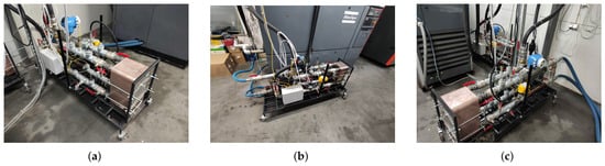
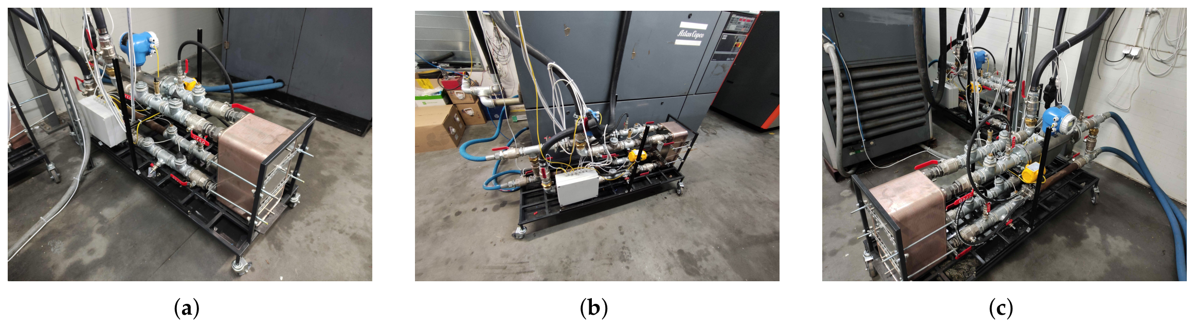
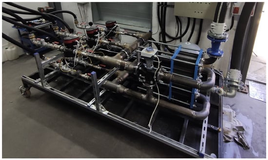
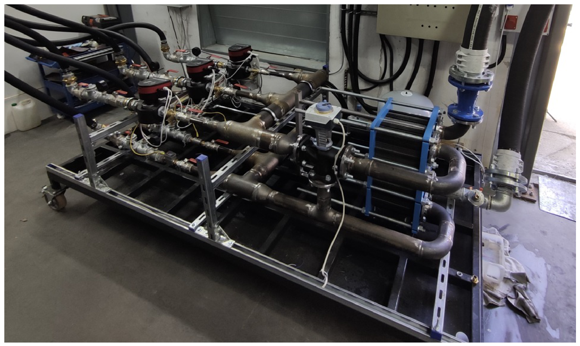
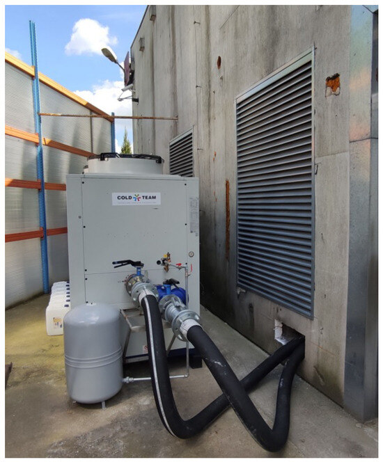
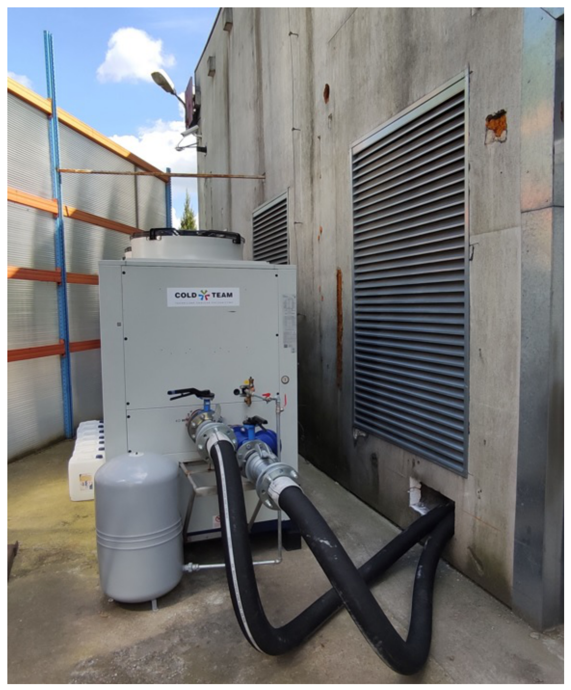
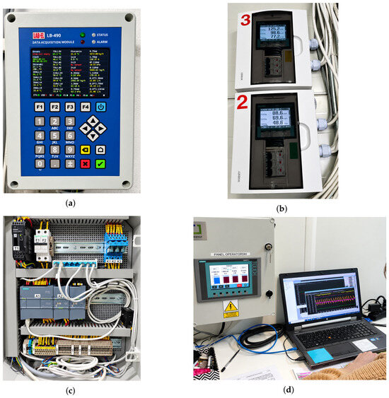
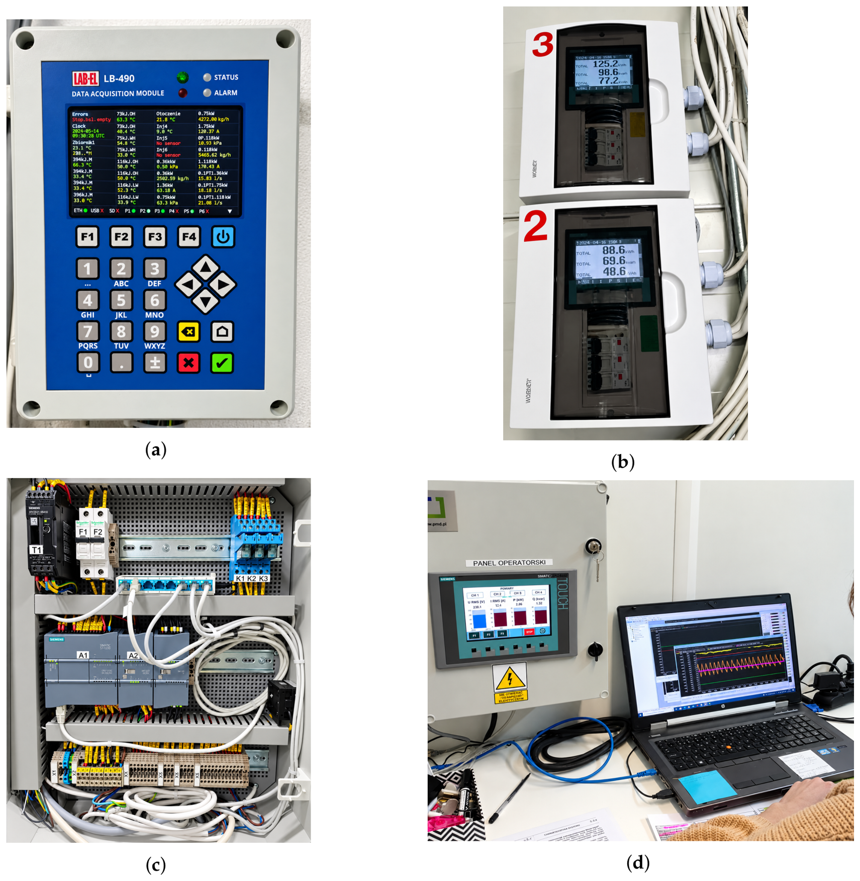
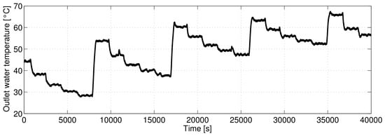
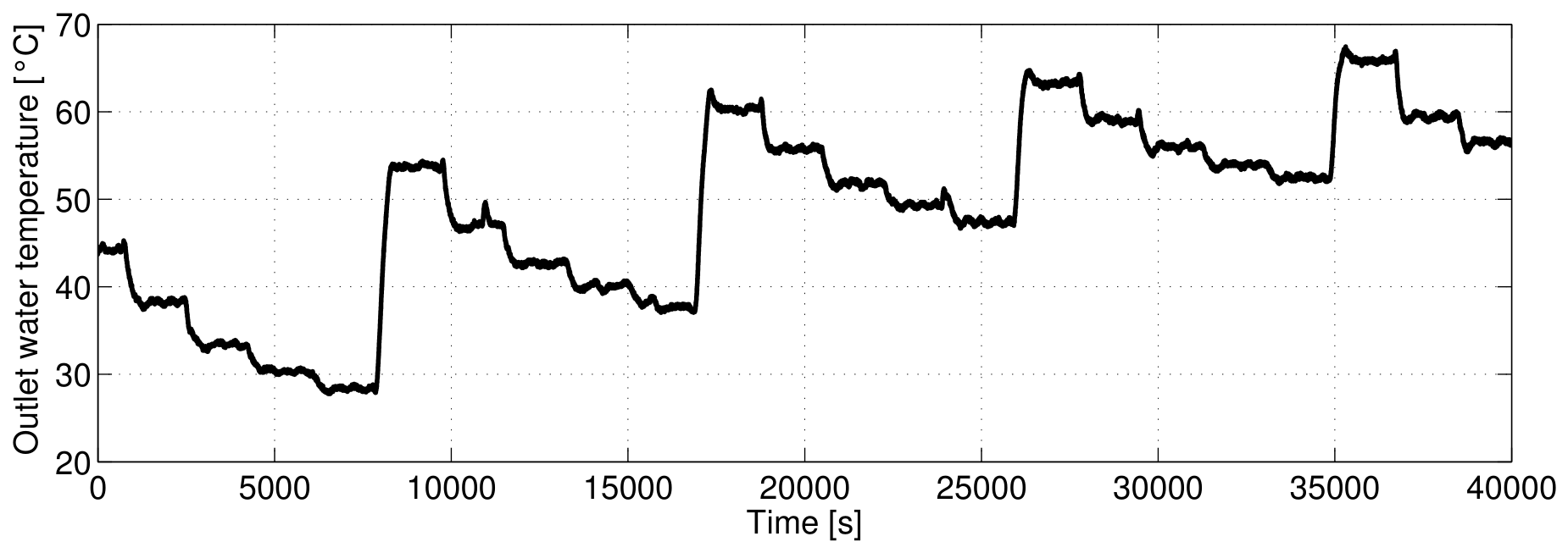
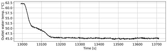
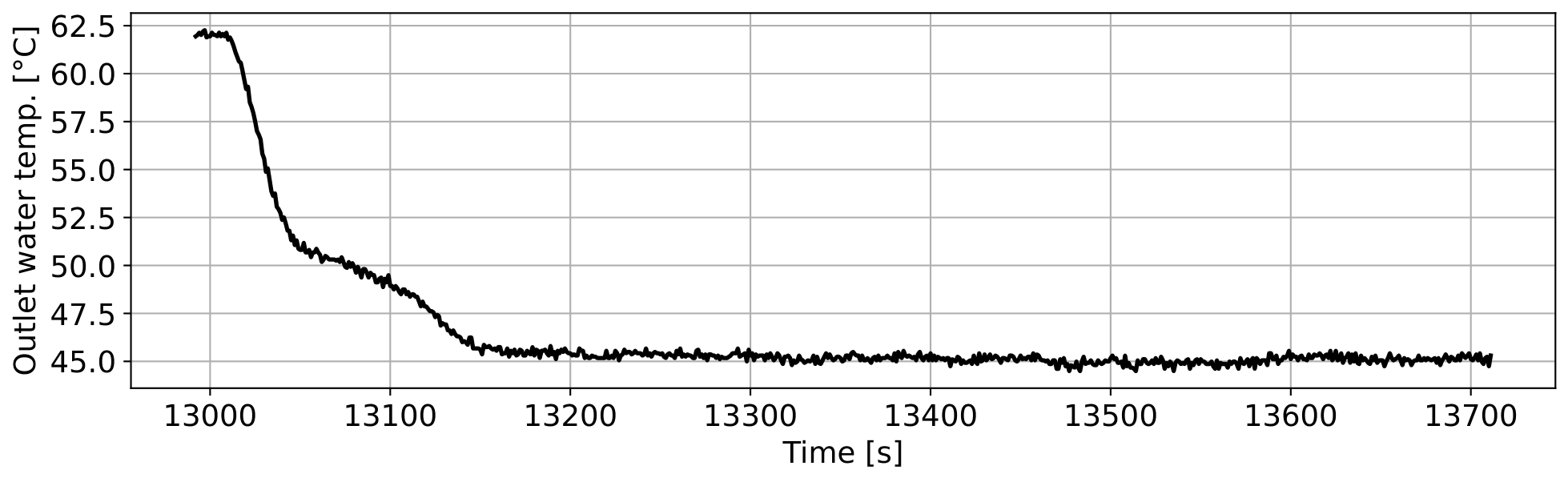
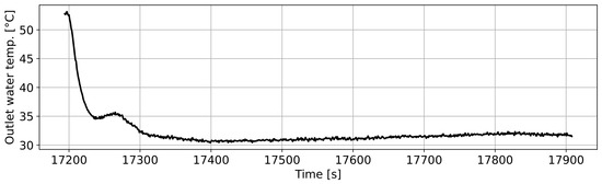
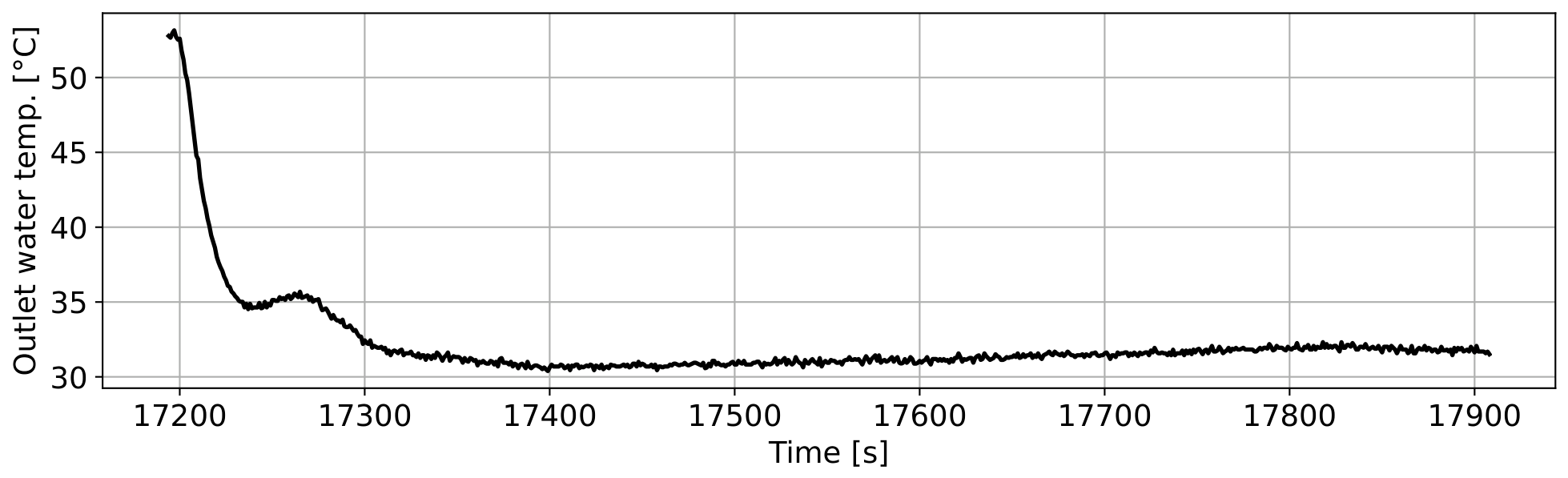
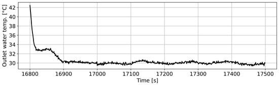
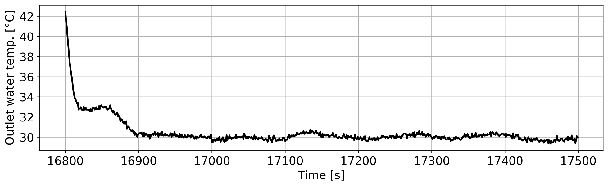
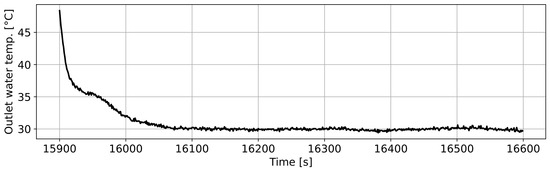
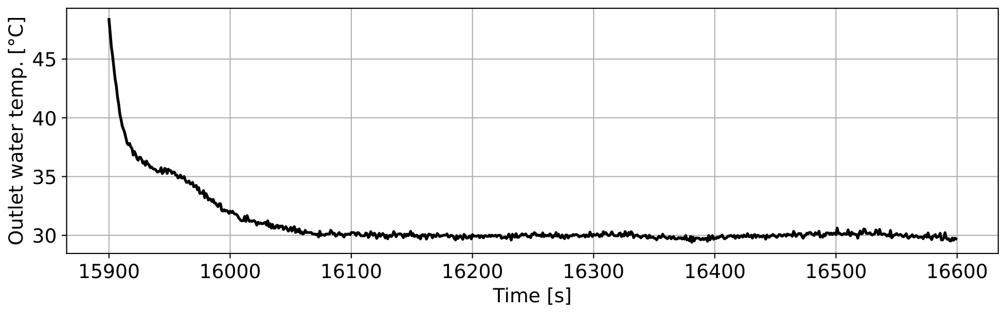
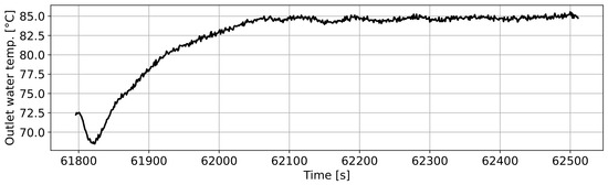
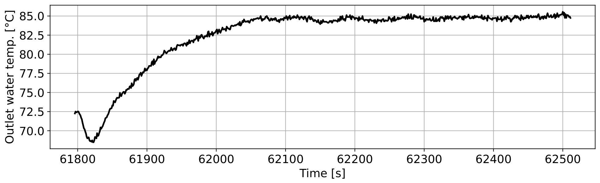
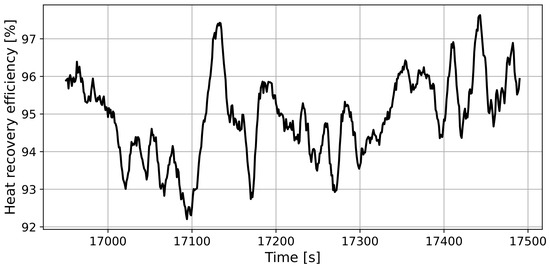
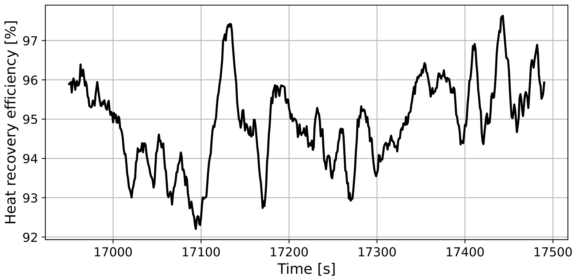

Disclaimer/Publisher’s Note: The statements, opinions and data contained in all publications are solely those of the individual author(s) and contributor(s) and not of MDPI and/or the editor(s). MDPI and/or the editor(s) disclaim responsibility for any injury to people or property resulting from any ideas, methods, instructions or products referred to in the content. |
© 2026 by the author. Licensee MDPI, Basel, Switzerland. This article is an open access article distributed under the terms and conditions of the Creative Commons Attribution (CC BY) license.