


Abstract
In response to issues such as the susceptibility of single-feature correlation in phase identification for consumers in low-voltage feeder areas to measurement noise and synchronous changes in load, this paper proposes a two-stage method for phase identification of consumers in low-voltage feeder areas. In the first stage, complex admittance increments are constructed based on voltage, active power and reactive power data from smart meters, and consumers are classified into two groups—high-confidence and low-confidence. According to maximum correlation strength and the distinguishability of candidate phases, results are output directly for high-confidence consumers. In the second stage, a voltage–power residual model—which combines the consumer’s own power variations with those of the load power for the remaining candidate phases—is employed to perform selective verification of low-confidence consumers. Simulations on a 31-node radial feeder with 60 consumers showed that, in the baseline white-noise case, Stage 1 and the complete method achieved 98.3 % and 100 %, versus 91.1 % and 94.5 % for voltage- and power-correlation benchmarks. Robustness testing showed that, when white noise increased to 2 percent, the Stage 1 and overall accuracy rates remained at approximately 82.6 % and 83.2 %. For feed scales ranging from 31/60 to 200/400, the overall accuracy of the method fell from 97.2 percent to 86.2 percent, whilst the running time increased from 13 s to 79 s; when the feed scale was increased whilst the noise level doubled, the accuracy fell further to 76.1 percent. The simulations also demonstrated that confidence stratification can filter some potentially misclassified consumers into the low-confidence set; the second stage can then correct errors for those consumers with sufficient residual discriminability, whilst rejecting candidate results where evidence is insufficient.
1. Introduction
As new sources and loads—such as distributed photovoltaic systems, electric vehicles, energy storage and flexible loads—continue to be connected to low-voltage distribution networks, traditional low-voltage feeder areas are gradually exhibiting operational characteristics such as bidirectional power flow, increased load fluctuations and worsening three-phase imbalance. Accurately understanding the affiliation between customers and distribution transformers, as well as the phase information of customers, is a crucial foundation for conducting lean analysis of line losses in service areas, addressing three-phase load imbalance, fault location, voltage quality management and distribution network state estimation [1,2]. However, low-voltage distribution networks are characterised by a large number of customers, complex branch structures and frequent line modifications. During the processes of adding new customers, relocating existing ones and adjusting lines, discrepancies may arise between actual on-site connection relationships and the archived information held in GIS, PMS and marketing systems. Traditional methods rely on manual inspections, power line carrier communication or specialised identification equipment. These methods can provide relatively direct connection information, but they suffer from high implementation costs, significant on-site workloads and difficulties in maintaining up-to-date information. With the continuous improvement of Advanced Metering Infrastructure (AMI) and electricity consumption data collection systems, the use of time-series data—such as voltage, active power and reactive power—already available from smart meters to perform consumer attribution and phase identification without additional hardware has become an important research direction for topology awareness in low-voltage distribution networks. Recent research into distribution network topology learning has also demonstrated that combining smart meter data with the physical relationships of power flow can effectively enhance the ability to perceive the structure of distribution networks under conditions of limited metering resources.
In China, a considerable amount of research has been conducted on the relationship between households and distribution transformers in low-voltage distribution areas, as well as on consumer phase identification. Early studies primarily focused on the similarity, correlation and clustering characteristics of consumer voltage curves. Tang Donglai et al. [3] proposed a method for identifying the relationship between households and distribution transformers in township distribution areas based on spatio-temporal aggregated voltage curves, determining connection relationships by analysing the spatio-temporal variation characteristics of voltage between consumers and distribution transformers. Zhou Gan et al. [4] employed multi-feature symbolic aggregation approximation and hierarchical clustering methods to perform feature compression and relationship identification on consumer measurement sequences. Shi Ziyi et al. [5] utilised dynamic time-scaling distance to describe the similarity of consumer voltage sequences, and combined adaptive K-nearest neighbour anomaly detection with adaptive density peak clustering to sequentially achieve verification of household-to-transformer relationships and consumer phase identification. The aforementioned methods fully capitalise on the strong correlation between consumer voltage variations within the same supply area, enabling the identification of consumer connection relationships without the need for additional on-site hardware. With the development of data mining and artificial intelligence technologies, relevant domestic research has gradually shifted from single correlation coefficients and traditional clustering towards multi-feature fusion, deep learning and multi-stage identification. Ou Feng et al. [6] converted one-dimensional electricity consumption data into two-dimensional features using Gram’s angle field and, in combination with transfer learning, established models for identifying customer-to-transformer relationships and phase identification in low-voltage distribution networks. Yu Weikun et al. [7] addressed the issues of missing data and differences in customer features by employing dual-scale similarity and an improved DBSCAN algorithm for phase identification in low-voltage feeder sections. Ma Shang et al. [8] constructed a linear reverse power flow model based on smart meter data and achieved joint identification of the topology and line parameters in low-voltage distribution networks using an impedance distance matrix. Zeng Tong et al. [9] further integrated multiple types of electrical features, such as voltage and current, and utilised optimised support vector machines to classify the ‘household–transformer’ relationships. Bu Qiangsheng et al. [10], on the other hand, combined fast derivative dynamic time warping with K-median clustering to perform hierarchical identification of the ‘household–phase–transformer’ relationships within transformer districts.
Internationally, two main technical approaches—data-driven and physical model-driven—have also emerged for phase identification in low-voltage consumers and distribution network topology. Hoogsteyn et al. [11] conducted a systematic comparison of various methods for consumer phase identification based on voltage and power data from smart meters; their research indicated that voltage data generally possesses strong phase identification capabilities, whilst the integration of power information can further improve identification performance in certain scenarios. García et al. [12] employed Bayesian inference to calculate phase probabilities based on changes in consumer load and load variations across each phase feeder, enabling the identification results to include not only phase labels but also corresponding confidence levels. Such research demonstrates that the distinguishability of data varies significantly between different consumers, and applying a uniform, forced classification strategy to all consumers does not necessarily yield the same level of reliability. Recent international research aims to enhance the physical interpretability of identification results. It places greater emphasis on the physical power flow relationship between voltage variations and changes in consumer power. Flynn et al. [13] utilised smart meter data to estimate voltage sensitivity coefficients, whilst accounting for the impact of variations in the source-side voltage of distribution transformers on these estimates; they then performed topological reconstruction of radial distribution networks based on these results. Vanin et al. [14] embedded phase identification into a linearised state estimation model and solved for phase assignment using mixed-integer linear programming. Fang et al. [15] further established a voltage sensitivity estimation model for three-phase low-voltage networks, reconstructing the network topology whilst accounting for transformer voltage, unknown phase angles and neutral coupling. Liu et al. [16] combined open GIS information with measurements from a limited number of smart meters to perform joint correction of the topology and parameters of low-voltage distribution networks. García et al. [17] employed the wavelet transform to extract multi-resolution time-frequency features and analysed the topological identification performance under different measurement errors, observability levels, and distributed generation penetration. Kalinga et al. [18] used K-means to perform initial consumer phase identification and further utilised linear regression to obtain voltage–power sensitivities to validate the initial phase results. Liu et al. [19] proposed a confidence-aware topology identification method for low-voltage distribution networks. By combining weakly supervised learning with Dempster–Shafer evidence fusion, they obtained meter-level confidence scores, enabling low-confidence identification results to be filtered out separately for further processing. At the same time, recent research has made significant progress in areas such as phase identification, voltage sensitivity, and confidence-base. In data-driven identification, a Siamese neural network was proposed in [20] to learn load-profile similarity without stepwise subtraction, and a graph neural network was applied in [21] to identify consumer phases using synthetic and measured power profiles. However, these methods rely on large-scale labeled or synthetic training data and do not provide confidence assessment for individual consumers. A spectral clustering approach using Gaussian mixture model kernel optimization was proposed in [22], but it only uses voltage magnitude and does not evaluate identification reliability. While Mugerwa et al. [23] considered prosumer scenarios.
However, the aforementioned studies also present the following issues: Firstly, statistical methods such as correlation coefficients, DTW and clustering primarily rely on the similarity of individual voltage or power curves. When load behaviour across different phases is highly synchronised, when a consumer’s own load fluctuations are minimal, or when influenced by distributed photovoltaic systems and measurement noise, multiple candidate phases may exhibit similar statistical characteristics, thereby resulting in consumers that are difficult to distinguish reliably. Secondly, most data-driven methods directly output phase classification results based on final correlation scores or clustering labels. They do not give sufficient consideration to the reliability of the identification results. Even when confidence assessments are introduced, low-confidence results are often directly designated for on-site verification. Comprehensive power flow optimisation, state estimation and large-scale sensitivity matrix methods offer strong physical interpretability. However, their models and computational processes are relatively complex. A large number of ordinary consumers can already be reliably identified through statistical features. Therefore, performing complex physical calculations uniformly on all consumers would impose an unnecessary computational burden. A tiered identification mechanism is needed. In this mechanism, a simple statistical method handles the majority of easily identifiable consumers, whilst physical models are used only for difficult cases. How to construct such a mechanism is a key issue in balancing identification accuracy and computational complexity.
To address these issues, this paper proposes a two-stage method for phase-discrimination of consumers in low-voltage feeder sections, based on complex admittance increment correlation and voltage–power residual verification. Firstly, the three-phase equivalent complex admittances of the consumer and the distribution transformer are constructed using the root mean square voltage, active power and reactive power collected from smart meters. The increments in the consumer’s complex admittance and the transformer’s three-phase aggregated complex admittance are then centred and normalised; initial correlation scores for the consumer’s A, B and C phases are obtained through normalised cross-correlation. Secondly, a confidence evaluation mechanism is established by combining the maximum correlation strength with the score differences between the first and second candidate phases, thereby classifying consumers into two categories: high-confidence and low-confidence. For high-confidence consumers, the initial identification results are output directly; finally, for low-confidence consumers only, the changes in voltage at the consumer end are corrected using the changes in voltage at the candidate phase source end. Furthermore, the consumer’s own power increment and the aggregated power increment of the candidate phases are introduced to construct a joint voltage–power response model that simultaneously accounts for local load disturbances and overall load changes in the same phase. Secondary identification is performed by analysing the fitting residuals of different candidate phases using independent validation samples. The main contributions of this paper are as follows:
- (1)
- A two-stage framework is proposed that combines complex admittance increment correlation with a confidence-based hierarchical approach, enabling both the rapid identification of reliable consumers and the referral of only complex consumers to the physical verification stage.
- (2)
- A voltage–power residual model is established, which combines the consumer’s own power variations with the residual load of the candidate phase to enable selective verification of low-credibility consumers.
- (3)
- The method relies solely on conventional smart meter voltage and power data, without the need for synchronous phase angle measurements or signal injection.
The framework diagram is shown in Figure 1 below.
Figure 1.
Overall framework diagram.
2. Preliminary Identification of Consumer Phase Based on Complex Admittance Incremental Correlation and Confidence-Based Stratification
2.1. Equivalent Complex Admittance Models for Loads and Transformers
In low-voltage transformer districts, smart meters on the consumer side are typically capable of obtaining operational data such as the root mean square (RMS) voltage, active power and reactive power. Let there be a total of N consumers in the low-voltage sub-station; at sampling time t, the RMS voltage, active power and reactive power of consumer i are denoted by Ui(t), Pi(t) and Qi(t), respectively, where i = 1, 2, …, N and t = 1, 2, …, T. T represents the total number of sampling points within the entire observation time window. In this paper, the convention is adopted that load power consumption is positive; that is, when a consumer draws active power and inductive reactive power from the distribution network, Pi(t) > 0 and Qi(t) > 0.
The complex power of consumer i at time t satisfies:
Here, Si(t) represents the consumer’s reactive power, denotes the consumer’s voltage phasor, and denotes the consumer’s current phasor; j is the imaginary unit, satisfying j2 = −1; and is the conjugate of the consumer’s current phasor. Equation (1) is the standard definition of complex power in the sinusoidal steady state [24].
From Equation (1), we obtain,
Therefore, the equivalent complex admittance of consumer i is defined as,
Taking into account, the equivalent complex admittance of the consumer is:
In the equation, the unit of Yi(t) is the siemens (S); the real and imaginary parts reflect the equivalent conductance and equivalent admittance characteristics of the consumer load, respectively. As can be seen from Equation (4), the equivalent complex admittance of the consumer can be calculated directly from Ui(t), Pi(t) and Qi(t), which are collected by the smart meter, without the need to obtain the absolute voltage phase angles that are strictly synchronised across different smart meters; it is therefore more suitable for conventional AMI measurement conditions.
For three-phase measurements on the secondary side of a distribution transformer, let p ∈ {A,B,C} denote the candidate phase. The rms voltage, active power and reactive power of the pth phase of the transformer at time t are denoted by U0,p(t), P0,p(t) and Q0,p(t), respectively. The subscript ‘0’ is used to denote the measurement point on the secondary side of the distribution transformer.
As with the definition on the consumer side, the equivalent complex admittance of the pth phase of the transformer is expressed as,
In the equation, Y0,p(t) represents the aggregate equivalent complex admittance of the pth phase of the distribution transformer at time t. As can be seen from Equations (4) and (5), the complex admittance characteristics used in the subsequent phase identification process in this paper can all be calculated from conventional voltage and power measurements, thereby avoiding reliance on synchronous phase angle measurement equipment.
For consumers connected to the same supply phase, changes in their loads are collectively reflected in the variations in the total active power, reactive power and equivalent complex admittance of the corresponding transformer phase. Therefore, compared with the absolute magnitude of the admittance, the temporal variation characteristics of a consumer’s admittance are more directly correlated with the changes in the aggregated admittance of the phase to which they belong. Furthermore, there may be significant differences in the long-term average load levels between different consumers. For example, the equivalent admittance of high-power consumers is consistently higher than that of low-power consumers over the long term; however, this difference in absolute magnitude does not directly indicate the phase to which a consumer belongs. To mitigate the impact of consumers’ electricity consumption scale and slow-changing trends on phase identification, this paper employs the change in complex admittance between adjacent sampling instants as a dynamic feature.
ΔYi(t) = Yi(t) − Yi(t − 1)
Here, t = 2, 3, …, T. ΔYi(t) represents the change in the equivalent complex admittance of consumer i between two adjacent sampling instants.
Similarly, the aggregate complex admittance increment of the pth phase of the transformer is defined as
ΔY0,p(t) = Y0,p(t) − Y0,p(t − 1)
In the equation, ΔY0,p(t) describes the change in the aggregate load of the transformer’s pth phase between adjacent sampling instants.
If consumer i is actually connected to the pth phase, then changes in that consumer’s load will directly contribute to the change in the aggregate load of the transformer’s pth phase. Therefore, within a given time window, the change in the aggregate complex admittance of the pth phase can be approximated as,
In the equation, Ωp represents the set of consumers actually connected to phase p; αi,p is the equivalent contribution coefficient within the time window, used to comprehensively characterise the impact of factors such as changes in consumer load, node voltage variations, line voltage drops and network losses on the variation in the transformer-side aggregated complex admittance; and vp(t) is a comprehensive disturbance term arising from unmodelled load variations and measurement errors. It should be noted that Equation (8) is not a strict power flow equation, but rather an equivalent expression describing the statistical correlation between the increment in a consumer’s complex admittance and the increment in the aggregated complex admittance of the phase to which the consumer belongs; αi,p is not treated as a network parameter to be estimated subsequently. A similar linear regression model between transformer-end aggregate admittance and consumer-end admittances was constructed in reference [25], where the identification of consumer–transformer relationships was formulated as a regression residual minimisation problem. This confirms the physical plausibility of approximating the aggregated phase admittance as a linear combination of consumer admittances. Equation (8) does not require that the change in a single consumer’s complex admittance be exactly equal to the change in the aggregated complex admittance of the corresponding phase of the transformer; rather, it merely indicates that if a consumer belongs to a particular phase, the consumer’s dynamic load variation will contribute to the change in that phase’s aggregated quantity, and therefore the two typically exhibit a strong statistical correlation over a relatively long time window. Conversely, for phases to which the consumer is not connected, the load changes do not directly contribute to the formation of the corresponding phase’s aggregate admittance; consequently, under normal operating conditions, the degree of dynamic correlation is typically relatively weak. Based on this characteristic, this paper utilises the normalised complex correlation between the consumer’s complex admittance increment and the transformer’s three-phase complex admittance increments to achieve preliminary identification of the consumer’s phase.
2.2. Correlation Matrix of Normalised Complex Admittance Increments
In order to process the data across the entire time window in a uniform manner, for consumer i, the T − 1 complex admittance increments obtained from Equation (6) are arranged in chronological order to form a column vector:
Here, ℂ denotes the field of complex numbers.
Define the mean of the incremental complex admittance of consumer i over the entire time window as,
In order to remove the mean of the samples in the incremental sequence within this window, Δyi performs a centring operation:
In the equation, 1 ∈ ℝ(T−1)×1 is a column vector whose elements are all 1; zi represents the centralised complex admittance increment sequence for consumer i.
As electricity consumption varies between consumers, the magnitude of changes in admittance may differ significantly. To prevent high-load consumers from naturally achieving higher matching scores due to larger magnitude changes, the centralised sequences are further normalised using the L2 norm:
In the equation, ‖⋅‖2 denotes the norm of a vector; ε is a very small positive number introduced to prevent the denominator from becoming zero; and di is the standardised complex admittance increment eigenvector for consumer i.
The same method is applied to all three phases (A, B and C) of the transformer.
Firstly, the complex admittance increment sequence for the pth phase is expressed as,
Its mean is,
To further obtain the centred vector,
as well as standardised feature vectors,
To minimise redundant calculations for each consumer and each phase, the standardised feature vectors for all consumers are combined column-wise to form a consumer feature matrix:
In this case, D ∈ ℂ(T−1)×N. It combines the normalised eigenvectors of the three phases (A, B and C) of the transformer into:
Among these, D0 ∈ ℂ(T−1)×3. This allows the normalised complex correlation matrix between all consumers and the three phases of the transformer to be calculated in a single step:
R = max[0,Re(DHD0)]
In the formula, Re(⋅) denotes taking the real part of a complex number; max(0,⋅) denotes comparing each matrix element with 0 in turn and taking the larger of the two. Therefore,
The reason for using the non-negative real part max(0, Re(·)) rather than the magnitude of the complex correlation is that in-phase variations in consumer load contribute to the aggregate complex admittance of the corresponding phase in the same direction. A positive real correlation therefore indicates a physical in-phase contribution, whereas a negative real correlation indicates an opposite-phase contribution that should not be counted as supporting evidence. Taking the magnitude would incorrectly reward even completely opposite variations with a high score. By retaining only the non-negative real part, the in-phase components are preserved while the opposite-phase components are suppressed. A similar in-phase-correlation design has been adopted in correlation-based topology identification studies [26].
This can be expressed as:
Here, ri,p represents the normalised complex admittance increment correlation score between consumer i and the pth phase of the transformer.
2.3. Preliminary Classification of Consumer Types
It can be seen from Equation (21) that each consumer has three candidate relevance scores: A, B and C.
For consumer i, the relevance score vector is defined as:
In accordance with the principle of maximum likelihood, the preliminary phase identification result for consumer i is defined as,
In the equation, represents the initial phase classification of consumer i. However, if the maximum relevance score among the three candidate phases is very close to the second-highest relevance score, simply applying Equation (23) to force a maximum-value classification may lead to misclassification. Therefore, it is also necessary to further evaluate the reliability of the recognition results. To simultaneously evaluate the absolute degree of association between the consumer and the best candidate phase, as well as the degree of distinguishability between the first and second candidate phases, the three correlation scores for consumer i are ranked in descending order: . Here, denotes the maximum correlation score for consumer i, corresponding to the initial judged phase obtained from Equation (23); denotes the second-highest correlation score, i.e., the candidate phase most likely to be confused with the judged phase; and denotes the minimum correlation score.
First, the maximum relevance intensity is defined as:
ρi is used to assess whether there is a sufficiently clear dynamic association between the consumer and the best candidate phase.
The confidence level for distinguishing between consumer phases is further defined as:
In the formula, ε is a very small positive number introduced to prevent the denominator from becoming zero. As can be seen from Equation (25), when there is a significant difference between the maximum correlation score and the second-highest correlation score, ci is large, indicating that the optimal candidate phase has a clear advantage over the other candidate phases; when the two scores are very close, ci approaches 0, indicating that the consumer has a high degree of uncertainty between the two candidate phases.
Consequently, this paper does not use a single threshold directly to determine confidence levels, but instead considers both the maximum correlation strength and the discriminative power between candidate phases. A maximum correlation strength threshold τr and a confidence threshold τc are set. When consumer i satisfies both conditions ρi ≥ τr and ci ≥ τc, that consumer is defined as a high-confidence consumer. Accordingly, the set of high-confidence consumers is represented as,
H = {(i|ρi ≥ τr, ci ≥ τc}
In the formula, H denotes the set of consumers for whom relatively reliable phase-angle results can be obtained in the first stage through the correlation of complex admittance increments. The remaining consumers who do not meet this criterion are collectively classified as low-confidence consumers, whose set is denoted by,
L = N\H
Here, N = {1,2,…,N} denotes the set of all consumers in the substation area; the symbol ‘\’ denotes the set difference operation. It should be noted that a low confidence level does not necessarily mean that the preliminary phase identification result for a consumer is incorrect; it merely indicates that, at present, the statistical correlation features based on the increment in complex admittance do not provide a sufficiently clear advantage for making a definitive determination.
3. Second-Order Identification of Voltage–Power Residuals for Consumers with Low Confidence Levels
Section 2 obtained correlation scores between consumers and the three phases (A, B and C) of the distribution transformer based on features derived from the increments in complex admittance, and classified all consumers into a high-confidence consumer set H and a low-confidence consumer set L according to the maximum correlation strength ρi and the phase-identification confidence level ci.
For high-confidence consumers, their complex admittance increments already exhibit a distinct correlation advantage with a particular candidate phase; therefore, the initial phase determination results obtained in Section 2 are directly accepted. For low-confidence consumers, as the correlation scores for two or more candidate phases are relatively close, relying solely on the statistical correlation of complex admittance may easily lead to misclassification. To this end, this paper further utilises the physical response relationship between changes in consumer load and changes in node voltage to perform a secondary identification of low-confidence consumers.
3.1. Voltage Correction at the Consumer End for Low-Confidence Consumers
In low-voltage distribution networks, voltage variations at the consumer end are influenced by both fluctuations in the source voltage on the secondary side of the transformer and changes in line load. If phase identification is based directly on changes in consumer voltage, voltage fluctuations in the upstream grid may mask the local voltage response caused by changes in consumer load.
Therefore, for a consumer i with low confidence, the voltage change between adjacent sampling instants is first defined as,
ΔUi(t) = Ui(t) − Ui(t − 1)
For the pth phase on the secondary side of a transformer, the change in voltage is defined as,
ΔU0,p(t) = U0,p(t) − U0,p(t − 1)
For a consumer i with low confidence, we assume that the consumer is connected to phases A, B and C, respectively, and use the changes in transformer voltage for the corresponding candidate phases to correct the source-end voltage. The correction voltage change for consumer i under candidate phase p is defined as,
In the equation, represents the change in the consumer’s local voltage—after accounting for the change in the common voltage at the source end of the transformer for that phase—assuming that consumer i is connected to phase p. Equation (30) is primarily used to mitigate the impact of fluctuations in the common voltage at the source end of the transformer on changes in the consumer node voltage. It should be noted that when the source-end voltage variations across the three phases are relatively close, relying solely on source-end voltage correction is insufficient to generate stable candidate phase discrimination information. Therefore, this paper further introduces the candidate phase aggregate power variation to characterise the combined effect of load variations from other consumers in the same phase and voltage drops across shared lines on the target consumer’s node voltage.
Define the change in active power for consumer i between adjacent sampling instants as,
ΔPi(t) = Pi(t) − Pi(t − 1)
The change in reactive power is,
ΔQi(t) = Qi(t) − Qi(t − 1)
Similarly, the changes in active power and reactive power at the transformer terminals between adjacent sampling instants are given by,
ΔP0,p(t) = P0,p(t) − P0,p(t − 1)
ΔQ0,p(t) = Q0,p(t) − Q0,p(t − 1)
Compared with changes in the power of an individual consumer, changes in the aggregated power of candidate phases can better reflect changes in the loads of other consumers in the same phase, as well as overall power disturbances along the shared supply path.
ΔP−i,p(t)=ΔP0,p(t)−ΔPi(t)
ΔQ−i,p(t)=ΔQ0,p(t)−ΔQi(t)
Here, ‘−i’ represents the equivalent residual load change obtained by subtracting the target consumer’s own power change from the aggregate power change of the candidate phase, assuming that consumer i belongs to candidate phase p. It should be noted that, as the aggregate power on the transformer side also includes line losses, ΔP−i,p(t) and ΔQ−i,p(t) are not, strictly speaking, the sum of the power increments of the remaining consumers, but rather equivalent proxy variables used to describe the overall change in the residual load of the candidate phase.
When a consumer’s load remains virtually unchanged between adjacent time steps, the corresponding voltage response contains little useful identification information. To enhance the effectiveness of secondary identification for consumers with low confidence levels, this paper selects only those time intervals where the consumer’s load change is relatively pronounced for subsequent calculations. The amplitude of the comprehensive load change for consumer i is defined as,
In the equation, Ai(t) describes the overall rate of change of the consumer’s active and reactive power at time t.
It is defined as,
τA,i = Q0.75(Ai)
Τi = {(t|Ai(t) ≥ τA,i}
In the equation, Τi represents the set of valid sampling times used by consumer i for secondary identification; τA,i is the adaptive load variation amplitude threshold for consumer i; and Q0.75(Ai) represents the 75th percentile of sequence Ai(t). By filtering out time points where the load remains essentially constant using Equation (39), samples with low information content can be eliminated, thereby reducing the distortion of the relationship between load variation and voltage response. The 75th percentile is selected as a compromise between two requirements. On the one hand, samples in which the consumer load is nearly constant carry little information about the voltage–power relationship and should be excluded. On the other hand, the retained samples must be sufficient for the subsequent 70/30 chronological training/validation split and for estimating the four response parameters. A substantially lower percentile would retain too many uninformative samples, whereas a substantially higher percentile would leave too few valid samples.
In the equation, and represent the training sample set and the validation sample set, respectively. In this paper, the first 70 percent of the valid time cross-sections are allocated to the training set and the remaining 30 percent to the validation set in chronological order; the training set is used solely for estimating response parameters, whilst the validation set is used solely for evaluating the residuals of candidate models, in order to avoid using the same samples for both parameter fitting and model performance evaluation.
In low-voltage radiation-type distribution networks, when operational conditions change only slightly between adjacent sampling instants, the relationship between voltage variation at the consumer end and load power variation can be approximated by a local linear relationship. For a consumer i with low confidence, assuming that the consumer is connected to phase p, the following voltage–power response model is established:
In the equation, k1,i,p and k2,i,p represent, respectively, the equivalent response coefficients of the target consumer’s own active and reactive power variations to its terminal voltage; k3,i,p and k4,i,p represent, respectively, the equivalent response coefficients of the active and reactive power variations in the remaining loads in the candidate phase to the target consumer’s terminal voltage; and εi,p(t) is a comprehensive error term resulting from factors such as local linearisation error, line loss approximation error, candidate phase aggregation proxy error and measurement noise.
When a consumer’s active or reactive load increases, the line current typically increases accordingly, leading to a drop in the consumer’s terminal voltage; hence, km,i,p ≥ 0, m = 1, 2, 3, 4 applies. For each consumer with low confidence, Equation (41) is established separately for phases A, B and C, thereby obtaining voltage–power response models corresponding to the three candidate phases. The four-term structure of Equation (41) reflects two physically distinct contributions to the consumer-side voltage variation. The first two terms, −k1,i,pΔPi(t) and −k2,i,pΔQi(t), describe the voltage drop caused by the consumer’s own load change through the local impedance of its connection branch. The last two terms, −k3,i,pΔP−i,p(t) and −k4,i,pΔQ−i,p(t), describe the additional voltage drop on the shared supply path caused by the simultaneous load changes of the other consumers connected to the same candidate phase. Separating these two contributions is essential: a consumer whose own load changes only weakly would otherwise be indistinguishable from the aggregated load variation of the phase, whereas including the residual phase load allows the shared-line coupling to be explicitly accounted for. Consequently, k1,i,p − k4,i,p are equivalent composite response coefficients that absorb the electrical distance, line impedance and network topology, rather than physical impedances to be estimated directly.
3.2. Joint Response Parameter Estimation and Residual Classification for Candidate Models
On the set of valid time slices for consumer i, the least-squares criterion is used to estimate the active and reactive voltage sensitivity parameters corresponding to candidate phase p. The optimisation model is as follows:
The non-negativity constraint in Equation (42) follows directly from the physics of the radial feeder: when the consumer’s load (or the residual phase load) increases, the line current increases and the consumer’s terminal voltage decreases, so all four response coefficients must be non-negative. Enforcing this constraint through non-negative least squares (NNLS) prevents the estimator from assigning physically meaningless negative coefficients that would artificially reduce the training residual. The parameters are estimated solely on the first 70% of the valid time samples in chronological order, while the remaining 30% are reserved as an independent validation set; this split avoids evaluating the model on the same samples used for fitting, which would otherwise underestimate the residual and overstate the confidence of the secondary identification.
Equation (42) enables consumer load variations to explain, as far as possible, the changes in consumer voltage—after correction for the candidate phase source voltage—by identifying a set of non-negative sensitivity parameters.
For the consumer’s actual connection phase, there is a genuine shared supply path coupling relationship between the load variations of the remaining candidate phases and the target consumer node voltage; consequently, the response parameters estimated from the training samples should exhibit good explanatory power on the independent validation samples. For erroneous candidate phases, there is no such electrical coupling relationship between their aggregated load changes and the target consumer node voltage; consequently, the prediction residuals on independent validation samples are typically large. After obtaining the sensitivity parameters corresponding to each candidate phase using Equation (42), the root-mean-square fitting residual of consumer i for phase p is defined as,
In the equation, represents the number of validation time slices for consumer i, and Ei,p represents the root mean square validation residual of the joint response model for consumer i under candidate phase p. The smaller the value of Ei,p, the greater the explanatory power of candidate phase p for changes in the consumer’s node voltage, and the higher the consistency with the consumer’s actual connection phase.
Therefore, based on the principle of minimum residuals, the secondary identified phase for consumer i with low confidence is defined as,
In the equation, represents the secondary phase identification result obtained for consumer i following voltage–power residual analysis.
3.3. Evaluation of Confidence Levels in Secondary Recognition
Simply selecting the phase corresponding to the minimum residual does not guarantee that the result is sufficiently reliable. When the fitting residuals for two candidate phases are very close, this indicates that the available measurement data is still insufficient to effectively distinguish the consumer’s true phase. Therefore, the residuals obtained for consumer i for the three phases A, B and C are ranked in ascending order as , where represents the minimum fitting residual, corresponding to the secondary recognition phase obtained from Equation (44); denotes the second-smallest fitting residual; and denotes the largest fitting residual.
The secondary identification confidence level for consumer i is defined as,
In the equation, ε is a very small positive number introduced to prevent the denominator from becoming zero. The secondary confidence is non-negative and quantifies how clearly the best candidate phase outperforms the second-best one in terms of the validation residual. When the minimum residual is much smaller than the second-smallest , is close to 1 and the best candidate has a clear physical advantage; when and are nearly equal, approaches 0, indicating that the two candidate phases are statistically indistinguishable given the available data. A fixed threshold τ2 is therefore imposed, and the secondary result is accepted only when . If , no forced determination is made and the consumer is marked as pending verification, because accepting an unreliable secondary result could incorrectly override a correct Stage-1 assignment.
The rejection criterion is twofold. First, if the number of valid time sections is less than Nmin, the response model cannot be reliably estimated, and the consumer is directly marked as pending manual verification without entering Stage 2. Second, even if enough valid samples are available, the Stage 2 candidate phase is accepted only if . When , the residual difference between the best and second-best candidate phases is insufficient to support a reliable decision. In this case, the Stage 2 candidate result is rejected, and the consumer is marked as pending manual verification rather than being forced into a phase. The Stage 1 result is not automatically retained either, because the low-confidence status in Stage 1 already indicates that the statistical correlation alone is not sufficiently discriminative. Therefore, no forced determination is made, and the consumer is referred for further manual inspection.
The final set of consumers pending verification is defined as,
Here, Nmin is the minimum number of valid time intervals required for the second-stage recognition. If |Τi| < Nmin, the number of valid samples is insufficient to estimate the voltage–power response model reliably, nor is it possible to compare the residuals of the three candidate phases with sufficient confidence. In such cases, a second-stage decision is not enforced, and the consumer is flagged as ‘pending manual verification’. U denotes the set of consumers for whom a reliable phase classification result cannot be obtained even after two-stage recognition.
Consequently, the final consumer phase classification rule in this paper is uniformly expressed as,
In the above equation, PMV refers to data pending manual verification.
Consequently, this paper proposes a two-stage mechanism for distinguishing consumer phases: first, complex admittance increment correlation features are utilised to perform rapid preliminary identification of all consumers; consumers are then categorised into high- and low-confidence groups based on maximum correlation intensity and candidate phase distinguishability, with initial identification results output directly for high-confidence consumers; subsequently, focusing solely on low-confidence consumers, the influence of common voltage fluctuations at the candidate phase source is mitigated, and a local voltage–power response model is established by combining the consumer’s own power variations with those of the remaining loads on the candidate phase. By comparing the prediction residuals of the three candidate phases (A, B and C) on independent validation samples, secondary identification of low-confidence consumers is achieved. consumers for whom there are insufficient valid samples or whose secondary identification confidence remains low are retained as subjects requiring further verification. The algorithm flowchart is shown in Figure 2 below.
Figure 2.
Algorithm Flowchart.
4. Simulation Analysis
4.1. Simulation Systems and Parameter Settings
This paper constructs a low-voltage transformer district sub-area comprising one distribution transformer, 31 low-voltage nodes and 60 single-phase consumers. The 60 consumers are randomly distributed across the nodes of the low-voltage network, with 22, 20 and 18 consumers in phases A, B and C, respectively. The rated line voltage on the secondary side of the distribution transformer is 400 V, and the phase voltage is 230 V. Consumer loads are constructed using typical residential load curves, with individual consumer variations and random household appliance start–stop events superimposed on the general daily load variation trend, to ensure that different consumers share certain commonalities whilst retaining independent random variation characteristics. Trunk lines are characterised by r0 = 0.25 Ω/km and x0 = 0.08 Ω/km, whilst branch lines are characterised by r0 = 0.60 Ω/km and x0 = 0.08 Ω/km.That is, the resistance of the zero-sequence circuit in the main line is 0.25 Ω per kilometre, and the reactance is 0.08 Ω; the resistance of the zero-sequence circuit in the branch line is 0.60 Ω per kilometre, and the reactance is 0.08 Ω. The typical length of a trunk line is 10–30 m, and that of a branch line is 5–20 m. The sampling interval is 15 min, and the standard observation period is 7 days (with a maximum observation period of 30 days). Consumer loads are generated by combining residential daily load curves with individual AR(1) fluctuations and random appliance switching events. The power factor varies gradually between 0.90 and 0.99. Power measurements are subject to 1 percent noise. Network power flows are solved via forward/backward sweeps with a convergence tolerance of 10−6. Thirty independent tests were conducted using seed numbers ranging from 21 to 50. The confidence thresholds were set at τc = 0.425, τr = 0.20 and τ2 = 0.60. The training and validation sets were split chronologically in a ratio of 70 percent to 30 percent, with the 75th percentile of valid samples in the second stage. The sensitivity threshold experiments and simulation results are presented section by section below.
Given that both Phase 1 and Phase 2 of this study utilise incremental information from adjacent time steps, the temporal structure of measurement errors directly affects the signal-to-noise ratio of the differential features. Therefore, this study focuses on defining two representative scenarios for voltage measurement errors. Model A represents white-noise-dominated measurement errors, where independent random white noise with a standard deviation of 0.2 percent is added to the voltage measurements of consumers and transformers to simulate scenarios with strong short-term random measurement errors. Model B represents a measurement error dominated by fixed bias, with an overall measurement error level of approximately 0.2 percent; however, the primary component is the fixed calibration bias of the electricity meter, containing only a small amount of short-term random noise. As the fixed bias can be largely offset during the differential calculation between adjacent time steps, Model B corresponds to a higher signal-to-noise ratio for the differential quantities.
To simulate the actual fluctuation characteristics of the secondary-side voltage of a distribution transformer, independent fluctuations and slight static deviations for each phase are superimposed onto the common trend. Figure 3 shows the typical daily voltage variation curves for the source-side voltages of phases A, B and C. It can be seen that the overall trends of the three-phase voltages are relatively consistent, whilst retaining a certain degree of inter-phase variation, thereby providing fundamental measurement information for subsequent low-confidence secondary identification of consumers based on source-side voltage correction.
Figure 3.
Voltage variation curves at the source end for phases A, B and C on a typical day.
4.2. Hierarchical Analysis of Recognition Performance and Confidence Levels in the First Stage
4.2.1. Confidence-Level Stratified Threshold Sensitivity Analysis
In the first stage, preliminary phase identification results for consumers are obtained using the incremental correlation of complex admittance; however, forcing classification based solely on the maximum correlation score may result in consumers with weaker correlations or similar scores across different candidate phases being directly assigned to a specific phase, thereby increasing the risk of misidentification. To address this, this paper sets a maximum correlation intensity threshold τr and a confidence threshold τc. Setting the thresholds too low may improve the coverage of consumers with high confidence, but may result in some misclassified consumers being erroneously output as reliable results; conversely, setting the thresholds too high, whilst improving the purity of the high-confidence set and the ability to intercept erroneous samples, may cause a large number of consumers to be categorised into the low-confidence set, thereby increasing the processing workload in Stage 2. Consequently, to quantitatively analyse the impact of the two thresholds, this paper employs a single-parameter sensitivity analysis method, selecting the high-confidence Identification accuracy, Stage 1 erroneous sample capture rate, and high-confidence coverage as evaluation metrics. Among these, the high-confidence Identification accuracy reflects the reliability of recognition results within the high-confidence set; the erroneous sample capture rate indicates the proportion of all misclassified consumers in Stage 1 that are successfully assigned to the low-confidence set; the high-confidence coverage rate represents the proportion of consumers for whom phase classification can be completed directly without proceeding to Stage 2. Together, these three metrics reflect the actual performance of the confidence-based stratification mechanism. Figure 4 and Figure 5 show Sensitivity Analysis τr and Sensitivity Analysis τc, respectively.
Figure 4.
τr Sensitivity Analysis.
Figure 5.
τc Sensitivity Analysis.
With τc = 0.425 held constant, τr was scanned, and the results are shown in Figure 4. As can be seen from the figure, as τr gradually increases from 0.05, the Identification accuracy of the high-confidence set remains at a consistently high level and gradually stabilises. This indicates that raising the maximum correlation strength requirement can further exclude weakly correlated consumers, but has a limited impact on the accuracy of the high-confidence set, which already possesses a high degree of reliability. By contrast, the error sample capture rate increases significantly as τr increases. When τr is small, approximately 78 percent of Stage 1 erroneous consumers can be classified into the low-confidence set; when the threshold is increased to around τr = 0.20, the error sample capture rate rises to approximately 95 percent. Thereafter, as τr continues to increase, the error capture rate rises only slowly and gradually enters a saturation region. At the same time, the high-confidence coverage rate shows a marked downward trend. When τr is small, high-confidence consumers account for over 90 percent; whereas at τr = 0.20, the coverage rate is approximately 60 percent. If the threshold is further increased to above 0.3, the improvement in the error sample capture rate becomes relatively limited, whilst the high-confidence coverage rate continues to decline significantly. For example, when τr approaches 0.5, the high-confidence coverage has fallen to approximately 15 percent. It can thus be seen that an excessively large τr causes a large number of consumers who could have been reliably identified in the first stage to be classified into the low-confidence set, whilst the gain in error capture capability is already very limited. Therefore, taking into account the reliability of high-confidence results, the ability to intercept erroneous consumers, and the scale of subsequent processing, this paper selects τr = 0.20.
By further fixing τr = 0.20 and varying the phase-discrimination confidence threshold τc, the results of the sensitivity analysis are shown in Figure 5. As τc increases, the high-confidence Identification accuracy consistently remains above approximately 99 percent, indicating that the high-confidence set as a whole possesses high reliability in phase discrimination. At the same time, the Stage 1 error sample capture rate increases significantly as the threshold rises, whilst the high-confidence coverage gradually decreases. When τc is small, for example τc = 0.05, almost all consumers satisfy the confidence criteria, and the high-confidence coverage approaches 100 percent; however, the error sample capture rate is only approximately 35 percent. This implies that a large number of potential Stage 1 misclassifications may not be effectively filtered out. As τc increases, consumers with similar scores and insufficient phase discrimination are gradually assigned to the low-confidence set, and the error capture rate rises rapidly. When τc = 0.425 is set, the error sample capture rate reaches approximately 95 percent, whilst still maintaining a high-confidence coverage of around 60 percent. Upon further increasing τc, the error sample capture rate gradually approaches saturation—for example, ultimately rising to only about 99 percent—whilst the high-confidence coverage continues to decline from approximately 60 percent to around 20 percent. Consequently, excessively increasing τc significantly increases the number of low-confidence consumers, whilst the improvement in error capture capability is already limited.
Based on the sensitivity analysis outlined above, the selection of thresholds follows a systematic process. Firstly, the high-confidence identification accuracy must be no less than 98 percent. Secondly, amongst the feasible combinations, the false positive capture rate should be maximised. Thirdly, the high-confidence coverage rate should be maximised. Where the performance difference between two candidate thresholds is within 0.5 percentage points, the lower threshold should be prioritised to avoid over-rejecting consumers.
Applying this process to Figure 4 and Figure 5, τr = 0.20 and τc = 0.425 were selected. With this combination, the error capture rate reaches approximately 95 percent, the high-confidence coverage is approximately 60 percent, and around 24 consumers are referred to the second stage for further verification. The impact of thresholds on identification accuracy and the number of consumers proceeding to the second stage can be summarised as follows: increasing τr or τc improves the error capture rate but reduces high-confidence coverage and increases the number of low-confidence consumers proceeding to the second stage. Conversely, lowering the threshold allows more consumers to remain in the high-confidence set, but results in more misclassified consumers going undetected.
4.2.2. Sensitivity Analysis of the Length of Observational Data
As the first stage of this study involves phase identification based on the statistical correlation between time series of consumer admittance increments and the three-phase aggregate characteristics of the transformer, the number of observed samples will directly affect the stability of the estimated correlation characteristics. To analyse the impact of historical data length on phase identification performance, sensitivity analyses were conducted using observation windows of 1 day, 3 days, 7 days and 14 days, respectively; the results are shown in Figure 6.
Figure 6.
The impact of the observation window length on consumers: (a) Recognition performance (b) Number of consumers with low confidence.
As can be seen from Figure 6a, the Stage 1 phase classification accuracy increases rapidly as the observation window length increases. When using only one day’s historical data, the impact of individual consumers’ random load variations on the relevant features is relatively pronounced due to the limited number of valid samples, resulting in a Stage 1 classification accuracy of approximately 85.1 percent. When the observation window was extended to 3 days, the Identification accuracy improved to approximately 98.6 percent; when further extended to 7 days, the Identification accuracy reached 100 percent. When the observation window was subsequently increased from 7 days to 14 days, the recognition performance remained essentially unchanged, indicating that as time-series samples continue to accumulate, the incremental features related to complex admittance gradually stabilise, and the marginal benefit of further increasing the data length becomes very limited. Figure 6b further illustrates the variation in the number of low-confidence consumers under different observation windows. As the data length increases, the number of low-confidence consumers shows a continuous downward trend, decreasing from approximately 26 in the 1-day scenario to approximately 14 in the 3-day scenario, and further reducing to approximately 6 and 3 in the 7-day and 14-day scenarios, respectively. These results indicate that a longer observation window can effectively enhance the statistical stability of the features correlating consumers with their true access phases, thereby reducing the ambiguity in distinguishing between candidate phases and enabling more consumers to obtain reliable identification results in the first stage. Taking into account the balance between identification performance and historical data requirements, this paper ultimately selects 7 days as the standard observation window for normal scenarios.
4.2.3. First-Stage Recognition Performance Under Different Noise Structures
Volt-PCC and Pow-PCC are classic single-feature baseline methods that are widely used in low-voltage phase identification. Volt-PCC represents a method based on voltage correlation, whilst Pow-PCC represents a method based on active power correlation. Neither method requires training, prior knowledge of the network topology, nor additional data sources. They utilise the same smart meter measurement data as the method proposed in this paper and directly demonstrate the advantages of constructing complex admittance incremental features by jointly utilising voltage, active power and reactive power. In recent years, phase identification methods have developed rapidly, including Bayesian inference, K-means and graph neural networks, amongst others. However, Bayesian methods require prior distributions and may be sensitive to assumed noise models. K-means combined with linear regression requires careful selection of the number of clusters and feature scaling, and its performance depends on the initialisation. Graph neural networks and other deep learning methods typically require large-scale labelled or synthetic training data, lengthy training times, and the inclusion of topological priors as graph inputs. To evaluate the preliminary phase identification capability of the proposed multi-admittance increment-based method, this paper selects Volt-PCC and Pow-PCC as comparison methods. All methods utilised the same dataset and were tested over a 7-day observation window with 30 sets of independent random seeds. The proposed method was compared with the voltage-correlation-based Volt-PCC method and the power-correlation-based Pow-PCC method under two conditions: Model A, dominated by white noise, and Model B, dominated by fixed bias. All methods utilised the same consumer load, network topology and observation data to ensure the fairness of the comparison results. Figure 7 and Figure 8 show the phase identification accuracy rates of each method under the two measurement error structures, respectively.
Figure 7.
Comparison of accuracy rates for different phase identification methods: (a) Model A; (b) Model B.
Figure 8.
The effect of secondary recognition confidence threshold τ2 on Stage 2 acceptance accuracy and net error correction.
In the Model A white noise scenario, the recognition accuracies of Volt-PCC and Pow-PCC were 91.1 percent and 94.5 percent, respectively, whilst the Identification accuracy of Stage 1 in this paper reached 98.3 percent, representing improvements of 7.2 and 3.8 percentage points over Volt-PCC and Pow-PCC, respectively. These results indicate that, in the presence of strong short-term random noise, traditional methods that rely solely on the correlation of voltage or power sequences are susceptible to random disturbances. In contrast, this study utilises voltage, active power and reactive power to jointly construct complex admittance increment features, which can more fully characterise the dynamic relationship between the consumer and the candidate phase, thereby demonstrating superior resistance to random noise. Following confidence-based stratification and selective verification in the second stage, the identification accuracy of the complete two-stage method further reached 100.0% (it should be noted that, at this stage, consumers identified as ‘to be verified’ during the second-stage identification with low confidence are not counted as correct).
In the Model B scenario dominated by fixed bias, the Identification accuracy of both Volt-PCC and Pow-PCC was 97.6 percent, whilst both Stage 1 and the complete method proposed in this paper achieved 100.0 percent. Compared with Model A, the performance of traditional correlation-based methods in Model B has improved significantly. This is primarily because fixed measurement bias exhibits greater stability during time-series variations and causes less disruption to the correlation structure than independent random noise at each time step; consequently, traditional methods based on voltage or power correlation are also able to maintain high phase-discrimination accuracy. In this scenario, Stage 1 of this paper is still able to achieve 100 percent Identification accuracy, although the improvement relative to traditional methods is significantly reduced.
4.3. Analysis of Secondary Recognition Performance for Low-Confidence Consumers
The second stage focuses solely on consumers with low confidence scores identified in the first stage. In accordance with the methodology outlined in Section 3, local voltage–power response models are established for each of the three candidate phases (A, B and C), taking into account the combined effects of changes in the consumer’s own power and changes in the remaining loads of the candidate phase. The root mean square errors corresponding to the three candidate phases are then compared using an independent validation sample.
4.3.1. Analysis of Confidence Thresholds for Secondary Recognition
To avoid the candidate phase with the smallest verification residual being accepted unconditionally, this paper further sets a secondary identification confidence threshold τ2, such that the Stage 2 identification result is accepted only when holds. Figure 8 illustrates the impact of different values of τ2 on the Stage 2 acceptance accuracy and net error correction under short-observation stress scenarios. As τ2 increases, secondary recognition results with low discriminative power are gradually rejected, and the acceptance accuracy of Stage 2 results shows an overall upward trend; simultaneously, the net error correction gradually shifts from a distinctly negative value towards and into the non-negative region. This indicates that a smaller value of τ2 causes some unreliable Stage 2 results to erroneously override the results of the first stage, whilst raising the acceptance threshold can effectively reduce the risk of such erroneous corrections. When τ2 falls within the range of approximately 0.4 to 0.6, the net error correction is close to or reaches a non-negative level, whilst the acceptance accuracy continues to improve. Although further increasing the threshold can yield higher acceptance accuracy, it reduces the number of consumers accepted following secondary recognition, thereby weakening the practical error-correction function of Stage 2.
Based on the sensitivity analysis outlined above, the selection of τ2 follows a systematic process. Firstly, the net error correction must be non-negative; this means that the error introduced by the second-stage verification must not exceed the error it corrects. Secondly, amongst the feasible thresholds that satisfy this condition, the acceptance accuracy of the second-stage results must be maximised. Thirdly, the number of consumers accepted in the second stage must be maximised so that as many consumers with low confidence levels as possible can benefit from physical verification. Where the performance difference between two candidate thresholds is within 0.5 percentage points, the lower threshold is preferred to avoid rejecting too many consumers whose status might be corrected. Applying this process to Figure 8, τ2 is selected as 0.60. At this value, the net error correction is non-negative, the acceptance accuracy is high, and a sufficient number of consumers can still be accepted in the second stage. Balancing recognition reliability and net error correction benefits, this paper ultimately selects τ2 = 0.60 as the acceptance threshold for Stage 2 results.
4.3.2. Analysis of Typical Low-Confidence Consumers
To further illustrate the actual processing of low-confidence consumers within the proposed two-stage identification framework, this paper conducts a case study using two representative consumers selected from a 1-day short-term stress scenario; the results are shown in Figure 9 and Figure 10.
Figure 9.
Analysis of Case A: (a) First-stage analysis; (b) Second-stage analysis.
Figure 10.
Analysis of Case B: (a) First-stage analysis; (b) Second-stage analysis.
In Case A, the consumer was actually connected to Phase B, but Phase C had the highest correlation score in Stage 1; consequently, the preliminary identification result was Phase C. Although its maximum correlation strength met the threshold ρi = 0.23 > τr, the confidence level for distinguishing between the first candidate phase and the next-best candidate phase was only . Therefore, this consumer was classified into the low-confidence set and the Stage 1 result was not directly accepted. Upon entering Stage 2, the validation residual corresponding to Phase B was the smallest, and the secondary identification confidence met the threshold ; consequently, Phase B was accepted as the final determination, successfully correcting the misclassification from Stage 1.
In Case B, the consumer was actually connected to Phase A, and Stage 1 also classified it as Phase A. Although the Stage 1 result was correct, the phase discrimination confidence level was slightly below the set threshold; consequently, it was still classified into the low-confidence set for secondary verification. In Stage 2, Phase C had the smallest validation residual. If the decision were based solely on the minimum residual criterion, an erroneous Phase C candidate result would have been obtained. However, the consumer’s secondary identification confidence was only , which did not meet the Stage 2 acceptance criteria; consequently, this candidate result was rejected, and the consumer remained in a status pending further verification.
The two cases above demonstrate the ‘error correction’ and ‘rejection’ functions of the secondary identification mechanism, respectively. For consumers who were misclassified in Stage 1 but exhibit distinct voltage–power response characteristics, Stage 2 can achieve effective correction based on the validation residual, whereas for consumers for whom the phase with the smallest residual has changed but lacks sufficient discriminative power, the secondary confidence threshold prevents unreliable candidate results from being directly accepted. Consequently, the two-stage framework does not simply involve Stage 2 overriding Stage 1, but rather achieves selective verification of challenging consumers through confidence stratification and secondary acceptance thresholds.
4.4. Robustness and Scalability Analysis
To evaluate the robustness and scalability of the proposed method, we conducted additional experiments under different noise levels, missing data rates, observation windows and feeder scales. Table 1 summarises the identification accuracy under various interference conditions, including measurement errors dominated by white noise (Model A) and those dominated by a fixed offset (Model B), as well as different missing data rates. Table 2 presents the identification accuracy and the proportion of consumers with low confidence levels for different observation window lengths. Table 3 reports the identification accuracy and runtime for different feedline scales, where an asterisk (*) indicates a doubling of the noise level.
Table 1.
Identification accuracy under different disturbance conditions.
Table 2.
Identification accuracy under different observation-window lengths.
Table 3.
Identification accuracy under different feeder sizes.
As shown in Table 1, under the white noise conditions of Model A, the accuracy of Volt-PCC drops sharply from 98.9 percent at 0.1 percent noise to 47.5 percent at 0.5 percent noise, and falls further to 35.0 percent at 2 percent noise. Pow-PCC, on the other hand, demonstrates greater robustness; within the same noise range, its accuracy drops only from 100 percent to 80.4 percent. In contrast, the proposed Stage 1 maintains 100 percent accuracy at noise levels as high as 0.1 percent, gradually decreasing to 82.6 percent when noise reaches 2 percent, whilst the Full method achieves 100 percent at 0.1 percent noise and 83.2 percent at 2 percent. This is because, under the white noise conditions of Model A, independent random white noise is superimposed on the voltage measurements; as Volt-PCC utilises voltage increment data—where the signal resides in the voltage domain—the white noise directly contaminates the signal, causing the method to gradually fail. Under the fixed bias conditions of Model B, Volt-PCC’s accuracy drops from 97.6 percent at 0.2 percent bias to 60.2 percent at 0.5 percent bias, whilst Pow-PCC, Stage 1 and the Full method all maintain accuracy levels above 95 percent even at a bias of 0.5 percent. With regard to missing data under Model A, the accuracy of Stage 1 and the Full method declined only slightly from 96.8 percent and 97.2 percent, respectively, when missing data was 0 percent, to 91.4 percent and 91.4 percent when missing data was 30 percent. In contrast, the accuracy of Volt-PCC remained at around 88 percent–91 percent, whilst that of Pow-PCC fell from 95.1 percent to 89.0 percent. These results indicate that the proposed complex admittance incremental features and the two-stage framework exhibit good robustness against both white noise and fixed bias, and are insensitive to missing measurements.
Table 2 illustrates the impact of the observation window length on the results. When using only one day’s data, the accuracy of the first stage was 84.1 percent, whilst that of the full model was 84.7 percent; 42.2 percent of consumers were classified as low-confidence and sent to the second stage. Upon extending the observation window to 3 days, the accuracy of both the first-stage and full models increased to 98.6 percent, whilst the proportion of low-confidence consumers fell to 25.1 percent. When the observation window was extended to 7 days, both methods achieved 100 percent accuracy, and the proportion of low-confidence consumers fell further to 10.5 percent. When the observation window was extended to 14 days and 30 days, the accuracy remained at 100 percent, and the proportion of low-confidence consumers fell to 4.1 percent and 0.6 percent, respectively. These results indicate that a 7-day observation window offers good identification accuracy; however, to assess the effectiveness of the second-stage method proposed in this paper, the proportion of low-confidence consumers must not be too low. Therefore, this paper selects 7 days as the observation window.
Table 3 shows the scalability results for Model A under white noise conditions (0.2 percent), with feeder sizes ranging from 31 nodes/60 consumers to 200 nodes/400 consumers. As the feeder size increases, the accuracy of Volt-PCC drops sharply from 91.2 percent at 31/60 to 52.1 percent at 200/400. The accuracy of Pow-PCC fell from 95.1 percent to 86.2 percent, whilst Stage 1 dropped from 96.8 percent to 85.3 percent and Full from 97.2 percent to 86.2 percent. Running time increased from 13 s to 79 s, with the increase following a roughly linear relationship. When the noise level was doubled (marked with an asterisk), the performance of all methods declined further. For the 200/400 * scenario, Volt-PCC dropped to 44.9 percent and Pow-PCC to 73.7 percent, whilst both Stage 1 and Full fell to 76.1 percent. This indicates that the methods proposed in this paper possess acceptable scalability in real-world low-voltage substation environments. In large-scale scenarios (where the noise level doubles), accuracy decreases, primarily due to the accumulation of line impedance and voltage drops, which weakens the correlation between individual consumer admittance increments and the aggregated phase admittance. This suggests that the method proposed in this paper may not perform optimally in more complex feeder areas, such as those containing high-power non-linear loads, feeders with high photovoltaic (PV) penetration, or extreme conditions involving ageing lines or poor contacts. Future work should continue to investigate phase identification methods for complex distribution areas.
5. Conclusions
This paper addresses the issues of the difficulty in quantifying the reliability of statistical correlation methods for phase identification among consumers in low-voltage transformer districts, and the challenge of uniformly handling problematic consumers. It proposes a two-stage identification method based on the incremental correlation of complex admittance and voltage–power residuals. In the first stage, complex admittance increment features are constructed using conventional smart meter measurements of voltage, active power and reactive power, and consumers are stratified by confidence level based on maximum correlation strength and candidate phase discrimination; in the second stage, which targets only low-confidence consumers, source-end voltage correction, changes in the consumer’s own power consumption and changes in the load of the remaining candidate phases are introduced, and selective verification is performed using validation residuals and secondary confidence levels. Simulation results indicate that the proposed complex admittance increment method demonstrates varying degrees of advantage under different measurement noise structures: in the baseline white noise scenario, the recognition rates for the first-stage and full methods were 98.3 percent and 100 percent, respectively, whilst those for Volt-PCC and Pow-PCC were 91.1 percent and 94.5 percent, respectively. In the fixed-bias scenario, both methods achieved 100 percent, whilst the two baseline methods both achieved 97.6 percent. Robustness tests indicate that, under 2 percent white noise conditions, the accuracy of the first-stage and full methods is approximately 82.6 percent and 83.2 percent, respectively; with 30 percent missing data, it is approximately 91.4 percent and 91.4 percent. For feed scales ranging from 31/60 to 200/400, the accuracy of the full method decreased from 97.2 percent to 86.2 percent, whilst the running time increased from 13 s to 79 s; under 200/400 conditions with noise doubled, the accuracy of the full method fell to 76.1 percent. Consequently, the method proposed in this paper is better suited as a confidence-aware selective verification framework; however, the performance of its second stage remains subject to the length of the observation window and short-term measurement noise. In future work, it could be further validated using long-term measurement data from actual distribution areas to assess its applicability under different load structures, levels of distributed generation penetration, and on-site measurement error conditions. Furthermore, due to limitations on the number of consumers in the distribution areas, this study did not conduct experiments on more complex distribution areas; this represents a necessary step for future research.
Author Contributions
Conceptualization, K.Z., P.W., H.M., Y.J., S.H. and Q.X.; methodology, S.H.; software, Q.X.; validation, S.H., Q.X., P.W. and Y.J.; formal analysis, S.H.; investigation, Q.X.; resources, S.H., Q.X. and K.Z.; data curation, Q.X.; writing—original draft preparation, S.H., Q.X. and H.M.; writing—review and editing, Q.X.; visualization, S.H., Q.X. and K.Z.; supervision, S.H.; project administration, S.H. All authors have read and agreed to the published version of the manuscript.
Funding
This research received no external funding.
Data Availability Statement
The data presented in this study are available on request from the corresponding author.
Conflicts of Interest
Authors Kaizhong Zhang, Peng Wang, Hongxia Ma and Yan Jin were employed by the State Grid Linxia Power Supply Company. The remaining authors declare that the research was conducted in the absence of any commercial or financial relationships that could be construed as a potential conflict of interest.
References
- Liu, S.Y.; Zhang, T.H.; Lin, Z.Z.; Cui, X.; Ma, J. Key technologies and algorithms for data-enabled lean operation of low-voltage distribution and utilization systems. Autom. Electr. Power Syst. 2023, 47, 187–199. [Google Scholar] [CrossRef]
- Deka, D.; Kekatos, V.; Cavraro, G. Learning distribution grid topologies: A tutorial. IEEE Trans. Smart Grid 2024, 15, 999–1013. [Google Scholar] [CrossRef] [Scilit]
- Tang, D.L.; Li, Q.; Chen, Y.D.; Zhang, J.; Liu, Y.B.; Song, W.P. A method for identifying the household-transformer relationship in rural distribution station areas based on voltage spatiotemporal aggregation curves. Autom. Electr. Power Syst. 2023, 47, 86–96. [Google Scholar] [CrossRef]
- Zhou, G.; Mao, H.; Feng, Y.J.; Hua, J.M.; Zeng, Y. Household-transformer relationship identification method based on multi-feature symbolic aggregate approximation and hierarchical clustering. Autom. Electr. Power Syst. 2024, 48, 133–141. [Google Scholar] [CrossRef]
- Shi, Z.Y.; Xia, X.Y.; Liu, J.B.; Gu, Y.Y.; Wang, Y.L.; Hong, J.Y. Topology identification method for low-voltage station areas based on AKNN anomaly detection and ADPC clustering. China Electr. Power 2024, 57, 168–177. [Google Scholar] [CrossRef]
- Ou, F.; Luo, X.H.; Long, J.W.; Xu, C.; Lai, G.; Yang, H. Household-transformer relationship and phase identification method for low-voltage distribution networks based on graph transformation and transfer learning. Zhejiang Electr. Power 2024, 43, 95–103. [Google Scholar] [CrossRef]
- Yu, W.K.; Zhu, R.Y.; Chen, X.; Shang, J.; Bai, X.; Wang, H. Phase sequence identification method for low-voltage distribution station areas based on dual-scale similarity and improved DBSCAN algorithm. Electr. Power Constr. 2024, 45, 74–88. [Google Scholar] [CrossRef]
- Ma, S.; Wei, Z.N.; Huang, M.Y.; Zheng, Y.; Sun, G. Joint identification of topology and line parameters in low-voltage distribution networks based on smart meter data. Autom. Electr. Power Syst. 2024, 48, 60–70. [Google Scholar]
- Zeng, T.; Li, W.P.; Yang, Y.Y.; Wang, D.; Lin, J.; Wang, H. Household-transformer relationship identification method for low-voltage station areas based on multi-feature fusion and WOA-SVM algorithm. Electr. Power Inf. Commun. Technol. 2025, 8, 82–90. [Google Scholar] [CrossRef]
- Bu, Q.S.; Guo, Y.; Jing, J.P.; Yi, W.; Lü, P.P.; Zhuang, S. Identification method of household-phase-transformer relationship in distribution station areas based on FDDTW and K-median clustering. J. Electr. Power Sci. Technol. 2026, 41, 107–116. [Google Scholar] [CrossRef]
- Hoogsteyn, A.; Vanin, M.; Koirala, A.; Van Hertem, D. Low voltage customer phase identification methods based on smart meter data. Electr. Power Syst. Res. 2022, 212, 108524. [Google Scholar] [CrossRef] [Scilit]
- García, S.; Mora-Merchán, J.M.; Larios, D.F.; Personal, E.; Parejo, A.; León, C. Phase topology identification in low-voltage distribution networks: A Bayesian approach. Int. J. Electr. Power Energy Syst. 2023, 144, 108525. [Google Scholar] [CrossRef] [Scilit]
- Flynn, D.; Pengwah, A.B.; Razzaghi, R.; Andrew, L.L.H.; Flynn, D. An improved algorithm for topology identification of distribution networks using smart meter data and its application for fault detection. IEEE Trans. Smart Grid 2023, 14, 3850–3861. [Google Scholar] [CrossRef] [Scilit]
- Vanin, M.; Van Acker, T.; D’Hulst, R.; Van Hertem, D. Phase identification of distribution system users through a MILP extension of state estimation. Electr. Power Syst. Res. 2024, 229, 110107. [Google Scholar] [CrossRef] [Scilit]
- Fang, L.; Pengwah, A.B.; Andrew, L.L.H.; Razzaghi, R.; Muñoz, M.A. Three-phase voltage sensitivity estimation and its application to topology identification in low-voltage distribution networks. Int. J. Electr. Power Energy Syst. 2024, 158, 109949. [Google Scholar] [CrossRef] [Scilit]
- Liu, D.; Giraldo, J.S.; Palensky, P.; Vergara, P.P. Topology identification and parameters estimation of LV distribution networks using open GIS data. Int. J. Electr. Power Energy Syst. 2025, 164, 110395. [Google Scholar] [CrossRef] [Scilit]
- García, S.; Fresia, M.; Mora-Merchán, J.M.; Carrasco, A.; Personal, E.; León, C. A data-driven topology identification method for low-voltage distribution networks based on the wavelet transform. Electr. Power Syst. Res. 2025, 243, 111517. [Google Scholar] [CrossRef] [Scilit]
- Kalinga, T.; Banfield, B.; Knott, J.C.; Robinson, D.A. K-means clustering and linear regression for user phase identification, verification, and topology determination under varied smart meter penetration. Energies 2026, 19, 183. [Google Scholar] [CrossRef] [Scilit]
- Liu, S.; Deng, C.; Zheng, Z.; Zhu, Y.; Lu, H.; Liu, W. Confidence-aware topology identification in low-voltage distribution networks: A multi-source fusion method based on weakly supervised learning. Energies 2026, 19, 1503. [Google Scholar] [CrossRef] [Scilit]
- Liu, D.; Giraldo, J.S.; Palensky, P.; Vergara, P.P. A siamese neural network model for phase identification in distribution networks. Int. J. Electr. Power Energy Syst. 2025, 169, 110718. [Google Scholar] [CrossRef] [Scilit]
- Dande, C.S.C.; Efkarpidis, N.A.; Christen, M.; Ginocchi, M.; Monti, A. Consumer phase identification in distribution grids using Graph Neural Networks based on synthetic and measured power profiles. Energy AI 2025, 22, 100607. [Google Scholar] [CrossRef] [Scilit]
- Leal, P.C.; Carvalho, P.M.S. Spectral Clustering of Voltage Profiles for Phase Identification in LV Grids: Accuracy Gains from Kernel Optimization. IEEE Trans. Power Deliv. 2025, 40, 3401–3412. [Google Scholar] [CrossRef] [Scilit]
- Mugerwa, G.; Megahed, T.F.; Elsabrouty, M.; Abdelkader, S.M. Data-driven consumer-phase identification in low-voltage distribution networks considering prosumers. Front. Energy 2024, 18, 827. [Google Scholar] [CrossRef] [Scilit]
- Kundur, P.; Malik, O.P. Power System Stability and Control, 2nd ed.; McGraw-Hill Education: New York, NY, USA, 2022; ISBN 978-1-260-47354-4. [Google Scholar]
- Ma, S.; Zhang, K.; Wang, L.; Hou, S.; Xue, Q. Data-Driven Identification of Active Distribution Network-to-Customer Transformer Relationships: A Power Active Admittance Regression Method. Energies 2026, 19, 3805. [Google Scholar] [CrossRef] [Scilit]
- Xu, J.; Zhang, W. Identifying Topology of Low Voltage Systems via Incorporating Measurement Correlations. J. Phys. Conf. Ser. 2022, 2254, 012020. [Google Scholar] [CrossRef] [Scilit]
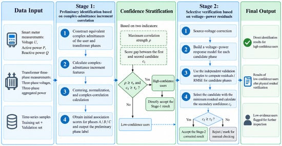
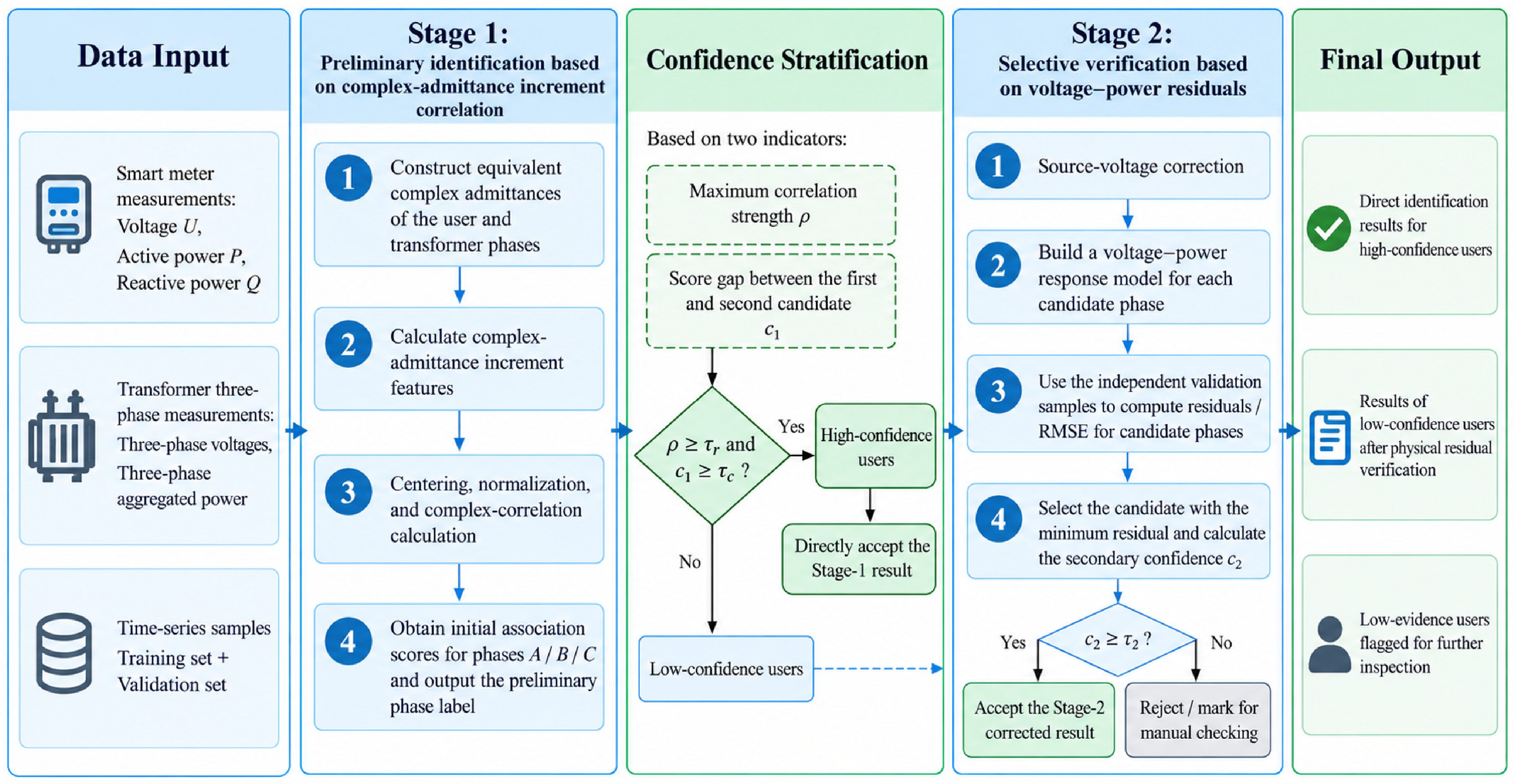
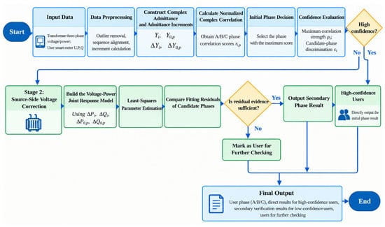
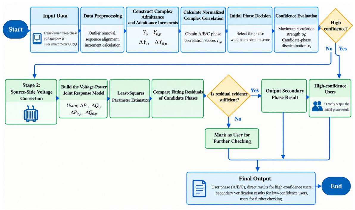
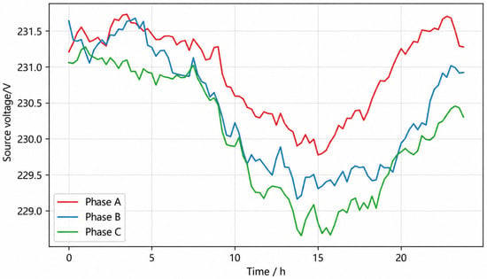
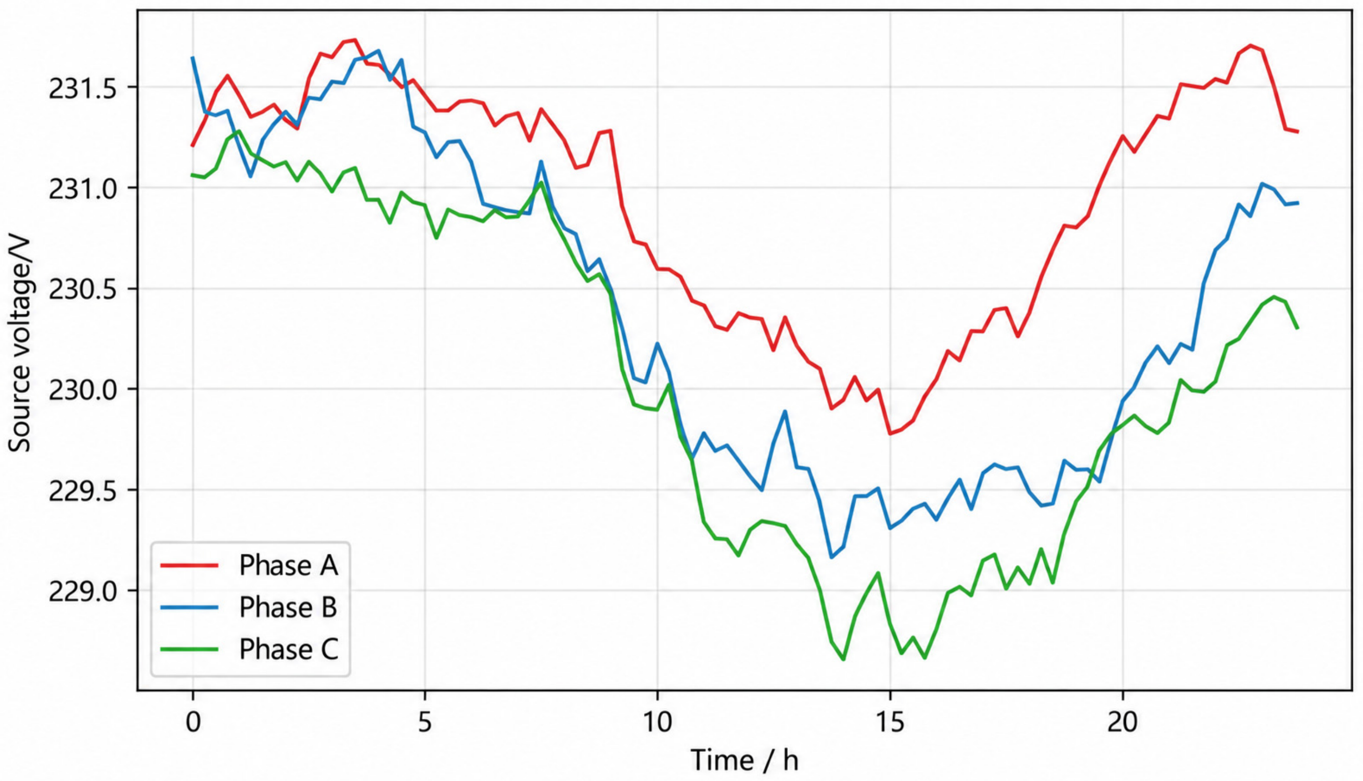
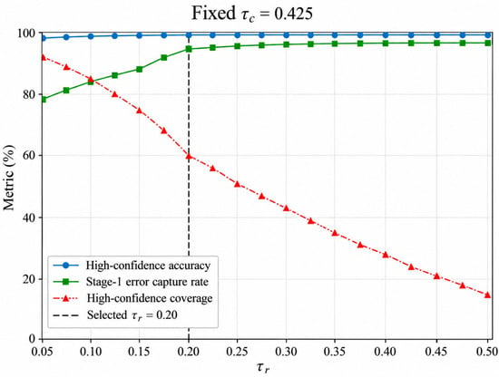
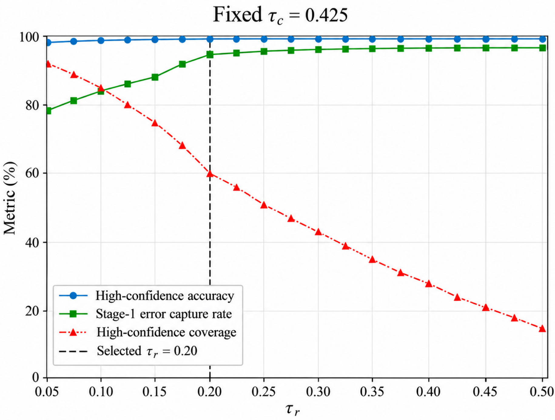
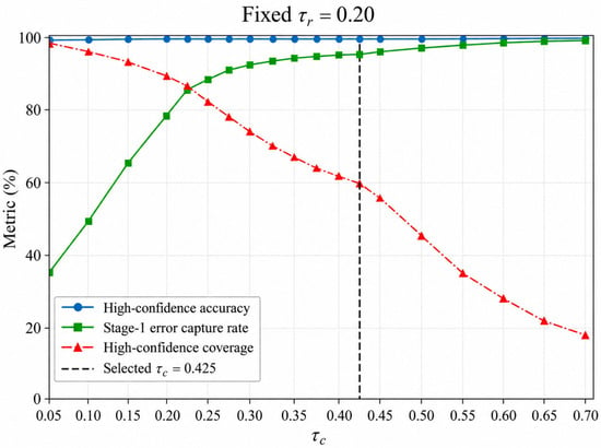
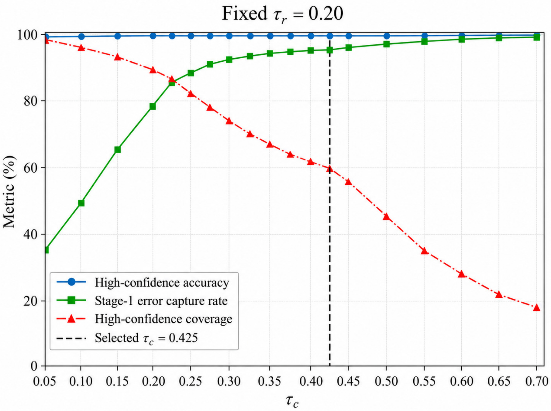
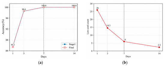
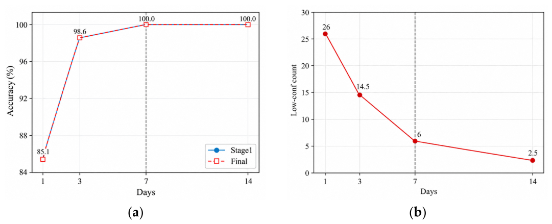
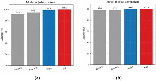
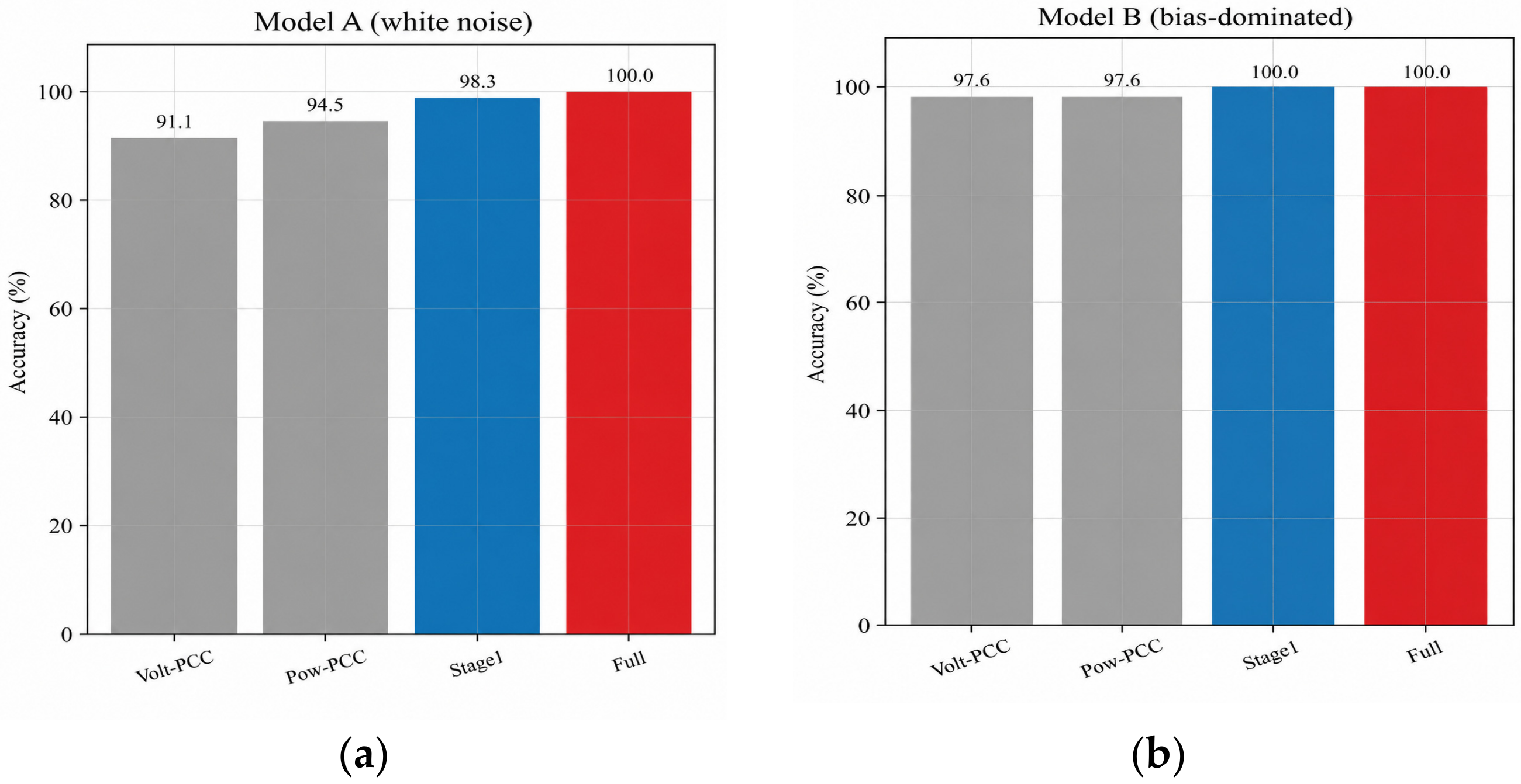
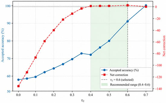
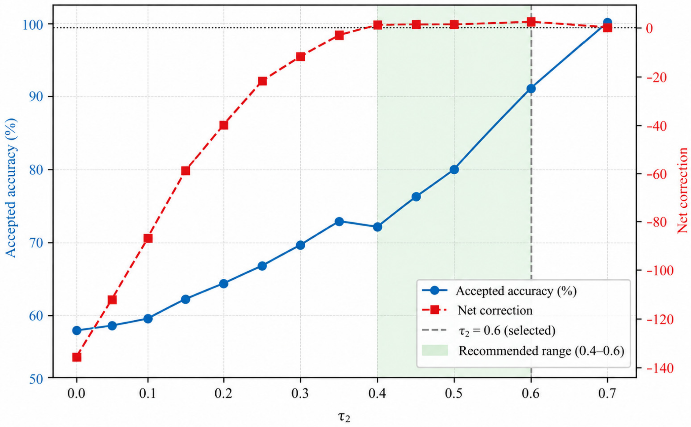
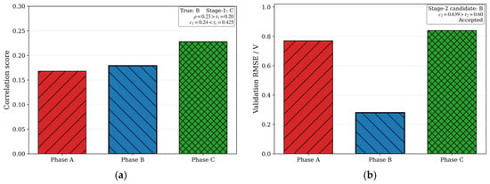
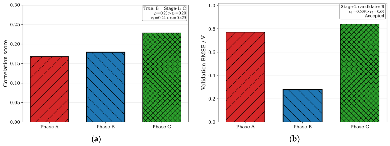
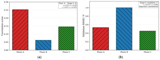
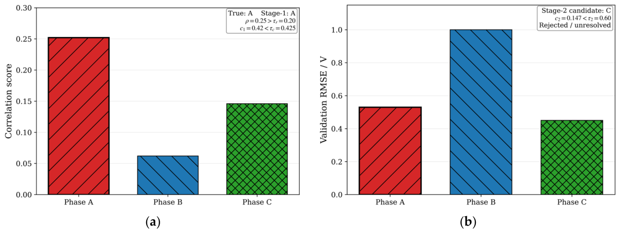

Disclaimer/Publisher’s Note: The statements, opinions and data contained in all publications are solely those of the individual author(s) and contributor(s) and not of MDPI and/or the editor(s). MDPI and/or the editor(s) disclaim responsibility for any injury to people or property resulting from any ideas, methods, instructions or products referred to in the content. |
© 2026 by the authors. Licensee MDPI, Basel, Switzerland. This article is an open access article distributed under the terms and conditions of the Creative Commons Attribution (CC BY) license.