


Abstract
High-frequency transient events in power systems are becoming increasingly significant due to lightning impulses, growing penetration of renewable energy sources, high-voltage direct current (HVDC) transmission systems, and power-electronic-interfaced equipment. Transformers operating in modern power systems, particularly those connected to power-electronic converters, HVDC systems and renewable-energy applications, may be exposed to steep-front voltage waveforms and high dv/dt stresses. These non-sinusoidal and repetitive transient conditions may cause severe dielectric stresses within transformer windings and insulation systems. High-frequency transformer models are therefore essential for analyzing transient behavior both at transformer terminals and within the windings. Such models consider winding geometry, electrostatic and electromagnetic couplings, and frequency-dependent parameters to represent transient voltage distributions with sufficient accuracy. Their reliability is critical for insulation coordination, transient overvoltage assessment, and transformer design. This paper presents a review of high-frequency transformer modeling approaches reported in the literature. White-Box, Gray-Box, and Black-Box models are examined together with analytical, finite element method (FEM)-based and measurement-based parameter extraction techniques. Time-domain and frequency-domain validation strategies are also discussed. Finally, the applicability, limitations, operational requirements, research gaps and future trends of existing modeling approaches are evaluated.
1. Introduction
Due to natural events and the growing use of power-electronic equipment in recent years, transformers are increasingly exposed to high-frequency (HF) transient voltages [1]. These transients arise from lightning impulse (LI), switching events, line faults/topology changes, harmonics, and ferroresonance, and they are generally aperiodic [2]. Following current interruption by vacuum circuit breakers, periodic transient waveforms may occur in the 10–200 kHz range. Very fast transient voltages (VFTOs) typically range from 0.5 MHz to 10 MHz and are predominantly observed in gas-insulated substations. The frequency ranges cited in this review should be interpreted as representative rather than universal boundaries. The dominant frequency regions and resonance locations may vary with transformer rating, winding geometry, terminal and grounding configuration, bushings, external connections, cables, and the measurement setup. Consequently, the required model bandwidth and spatial resolution should be selected based on the transient phenomenon and the quantities of interest.
Such transients affect operational safety and economics. Lightning and switching events impose insulation stress on transformers, which can lead to failures, thereby shortening or even ending their service life [3].
According to international standards, power transformers must be designed to withstand various transient voltages, such as LI and switching surges. In this context, manufacturers must conduct LI tests to assess the adequacy of the insulation system [4,5]. It was stated that, based on feedback from fault analyses, standard LI and switching impulse tests may not guarantee the dielectric strength of the transformer insulation system under all conditions [6,7]. Moreover, it is shown in [8] that HF waveforms other than the standard test shapes can excite winding resonances and produce higher internal voltages, underscoring the need to revisit standard impulse tests. To evaluate the transient voltage performance of the transformer, the system behavior—including the line, breaker, surge arrester, and transformer terminal equivalent circuit—should be modeled instead of applying standard impulse voltages (full wave, chopped wave, and switching impulses) directly to the transformer terminals. The transformer terminal voltage obtained from this model should be applied to the detailed HF transformer model. Studies in the literature include incorporating a transformer model into the power system, determining the terminal voltage, and then testing the transformer using this voltage value [9,10].
A detailed HF transformer model includes self and mutual inductances, capacitances and resistances [11]. When examining the historical development of detailed models, Abetti’s 1953 study [12] was the first to model capacitive effects between windings and the ground in transformer transient analyses with a separate equivalent circuit. Incorporating the capacitance network into the magnetic model produced a comprehensive electromagnetic equivalent circuit model. Neglecting mutual inductances in the equivalent circuit model results in errors in determining the natural frequency of the system. Abetti and Maginniss proposed a circuit model that included mutual inductances, which are often neglected [13]. The distributed-parameter method was used to model air-core and iron-core coils. Excellent fits were achieved up to the seventh harmonic in air-core coils and up to the third harmonic in iron-core coils. The 1957 study by McWhirter and colleagues, which determined the distribution of impulse voltages within transformer windings, surpassed previous intuitive and experimental studies by providing a systematic and numerical approach using detailed mathematical modeling and combined use of digital and analog computers [14]. Later, Dommel introduced the trapezoidal rule-based algorithm, which became the basis of EMT programs and allowed HF transformer models to be included in power system simulations [15]. Building on these developments, Vaessen created the HF equivalent circuit based on the transformer’s geometric parameters for use in the electromagnetic transient program (EMTP) [16]. Morched et al. used the frequency-dependent branch (FDB) element in the EMTP to model the frequency-dependent results obtained through terminal measurements and calculations [17]. A compilation study conducted by Martinez and Mork in 2005 addresses the classification, applicability, and limitations of transformer models that can be used in transient regimes that may occur between 1 Hz and 10 kHz [18]. The study provided guidance in selecting the appropriate transformer model for transient events. CIGRE technical documents classify HF transformer models into three main categories: White-Box, Gray-Box, and Black-Box [7]. The White-Box model is the most detailed, as it is designed based on the geometric and material properties of the transformer [19]. The applicable frequency range of a White-Box model is not defined by a universal upper frequency limit, but depends on the adopted spatial resolution, parameter representation, winding geometry, connection details, and physical phenomena to be reproduced. As frequency increases, insufficient segmentation, neglected parasitic couplings, and simplified representations of frequency-dependent losses may progressively reduce model accuracy. The Gray-Box model combines limited design information with frequency response measurements to obtain parameters, and it is generally applicable to wideband frequency response and HF-transient studies. The Black-Box approach relies solely on measurement data to represent the terminal behavior of the transformer and achieves high accuracy within the measurement band of frequency response analysis (FRA) tests, typically 20 Hz–10 MHz. Analytical formulas, finite element method (FEM) analyses, and measurement-based techniques have been developed to extract model parameters.
Although the White-Box model was able to estimate the maximum voltage stresses with reasonable accuracy, its reproduction of the waveform shape remained limited in [7]. It was emphasized that the inclusion of frequency-dependent damping is necessary to improve the agreement. Gray-Box models, although more attractive in terms of computational cost, exhibit limited accuracy. By contrast, Black-Box models perform well in terminal behavior. Therefore, the topic remains highly relevant, and research efforts are still ongoing.
Although numerous studies have investigated transformer behavior under transient conditions, review articles that specifically provide an integrated methodological synthesis of high-frequency transformer modeling are scarce. This review aims to provide a critical and comparative perspective on modeling techniques, parameter extraction methods, and validation procedures. This study was conducted as a structured narrative review to synthesize the representative literature on high-frequency transformer modeling rather than to provide an exhaustive systematic or bibliometric survey. The relevant literature was identified through searches of the Web of Science Core Collection, IEEE Xplore, ScienceDirect (Elsevier), and IET publications. The searches were conducted using combinations of terms, such as “high-frequency transformer modeling”, “transformer winding model”, “White-Box”, “Gray-Box”, “Black-Box”, “frequency response analysis”, “parameter extraction”, “finite element method”, “vector fitting”, “transient transformer model”, “lightning impulse” and “very fast transient overvoltage”. Because this study was a structured narrative review, no single fixed Boolean search string was applied; instead, related terms were combined iteratively according to the modeling approach, parameter-extraction method, and application examined. Peer-reviewed journal articles and relevant conference papers addressing HF transformer modeling, parameter extraction, transient analysis, or model validation were considered. Studies were prioritized when they explicitly addressed HF transformer model development, parameter determination, transient or frequency response analysis, or model validation. Publications focusing solely on general transformer operation or diagnostics, without a direct relationship to HF modeling, were not considered core modeling studies. IEEE and IEC standards, as well as CIGRE technical brochures, were included as technical reference documents. Foundational studies dating back to 1953 were retained to represent the historical development of the field, while recent publications up to 2025 were included to reflect contemporary modeling approaches. The literature search was updated during the revision process in September 2026. The final reference set comprised 103 sources, including journal articles, conference papers, technical standards, CIGRE technical brochures, and other relevant technical references.
While this review deliberately adopts the widely used terminology (i.e., White-Box, Gray-Box, and Black-Box) to ensure consistency with the relevant literature, it defines methodological boundaries and classifies the reviewed studies into these categories. Furthermore, this study compares parameter determination techniques, such as analytical, FEM and measurement-based techniques, by evaluating their computational trade-offs and identifying their valid frequency ranges. Ultimately, by evaluating the limitations of current modeling practices and identifying emerging research gaps, this review aims to offer useful guidance for future research.
Aim and Objectives of the Study
The primary aim of this study is to provide a structured review of HF modeling methodologies for power transformers, with particular emphasis on modeling approaches, parameter extraction techniques, and validation practices. Converter, HVDC, renewable energy, traction, and other special transformer applications are considered important contemporary application contexts and emerging research needs, rather than the exclusive scope of the review. Within this scope, the specific objectives of the study are as follows:
- To review and classify HF transformer modeling approaches reported in the literature under the three main categories of White-Box, Gray-Box, and Black-Box models, highlighting their underlying assumptions and levels of physical detail.
- To investigate parameter extraction techniques employed in HF transformer models, with a structured comparison of analytical methods, FEM-based approaches, and measurement-based techniques.
- To review and assess model validation practices, including time-domain and frequency-domain validation strategies, as well as commonly used experimental and numerical benchmarks.
- To analyze the application areas of different modeling approaches, clarifying for which phenomena and studies (e.g., lightning impulses, switching transients, VFTO, and FRA-based diagnostics) each model type is typically employed.
- To evaluate the modeling methodologies not only from the perspective of the academic literature, but also in the context of IEEE and IEC standards and CIGRE technical brochures, thereby linking research developments with industrial practice.
- To discuss observed trends within the literature considered in this review and future research directions in HF transformer modeling, identifying emerging challenges, open research gaps, and potential advancements in modeling and validation methodologies.
2. Modeling Approaches
Figure 1 shows the approach adopted for HF transformer modeling.
Figure 1.
HF transformer modeling approaches.
Figure 1 illustrates the primary taxonomy of high-frequency transformer modeling based on the modeling philosophy found in the literature. Modeling techniques are grouped into White-Box, Gray-Box, and Black-Box categories depending on the degree of physical representation, parameter determination strategies, and intended application areas. To further clarify the distinctions among these modeling families, Table 1 presents a comparative overview of their representation levels, parameter sources, and typical application areas.
Table 1.
Comparative overview of modeling approaches.
The most detailed HF model of a transformer is referred to in the literature as the White-Box model. It is the electromagnetic model that best represents the transformer, developed to calculate the voltages and currents within the transformer windings [7,20]. Constructing a White-Box model typically requires detailed manufacturer information, as the transformer’s internal geometry, insulation materials, and conductor properties must be thoroughly understood [21].
Consequently, these models are typically developed directly by or in close collaboration with the manufacturers. In physical practice, the dielectric withstand capability of transformer windings is verified by subjecting the transformer to standard full-wave, chopped-wave, and switching impulse voltages [22,23]. However, prior to conducting these physical tests, White-Box models are used to simulate these exact impulse conditions. This pre-test simulation enables the prediction of internal winding voltage distributions and localized insulation stresses. Such simulations also provide a basis for evaluating model accuracy by comparing outputs from different modeling approaches and, where available, measured responses. Even when different White-Box models are applied to transformers with the exact same geometry and material properties, the obtained results are not identical [7]. While these modeling results are generally sufficient for determining maximum voltage, it is important to examine the models in more detail due to ongoing inaccuracies in predicting resonance and damping points [24,25]. White-Box models are divided into two categories: lumped-parameter and distributed-parameter models [7].
The lumped-parameter model is based on the spatial separation of the windings [26]. Each section is modeled separately, and all subsections are combined to form a model [27]. Because the windings exhibit resistive and magnetic behavior, the circuit model is created using resistance (R), inductance (L), capacitance (C), and mutual inductance (M) elements [28]. The circuit equations are obtained by formulating differential equations in the time domain using Kirchhoff’s current and voltage laws. In this way, the magnetic and electrical interaction in the internal structure of the transformer is modeled [28,29,30,31]. The applicability of a lumped-parameter representation depends on the electrical length of the individual winding sections. When variations in voltage and current within a section can no longer be neglected, coarse segmentation may shift resonant frequencies and reduce the accuracy of predicted internal voltage distributions. Therefore, the required segmentation should be determined according to the frequency range and the quantities of interest rather than by a fixed frequency threshold.
In Figure 2, each winding is divided into N lumped segments, indexed by i = 1, …, N, resulting in N + 1 electrical nodes indexed by k = 0, …, N. Segment i is located between nodes i − 1 and i. Cg,1,k and Cg,2,k represent the winding-to-ground capacitances of the high-voltage (HV) and low-voltage (LV) windings at node k, respectively, while Gg,1,k and Gg,2,k represent the corresponding winding-to-ground conductances. C12,k and G12,k represent the inter-winding capacitance and conductance between the corresponding HV and LV nodes indexed by k. Cs,1,i and Cs,2,i represent the series capacitances associated with segment i, while Gs,1,i and Gs,2,i represent the associated dielectric-loss conductances. R1,i and R2,i represent the segment resistances, whereas L1,i and L2,i represent the corresponding self-inductances. The dots at the inductor terminals indicate the reference polarities for magnetic coupling, while the corresponding mutual-inductance terms between winding segments are incorporated into the inductance matrix.
Figure 2.
Sectional lumped-parameter representation of the HV and LV transformer windings, each divided into N lumped segments. Adapted from [31].
The circuit equations of the lumped-parameter model can be written in matrix form by applying Kirchhoff’s current and voltage laws. Using modified nodal analysis, the system can be expressed as shown in Equation (1).
where x(t) is the vector of MNA unknowns, comprising node voltages, inductor currents, and currents through ideal voltage sources, where present. Matrix G contains the algebraic contributions from resistive and conductive elements and circuit interconnections. Matrix C represents the dynamic part of the system and contains the capacitance and inductance blocks, including the mutual-inductance terms. Thus, C is a descriptor matrix rather than a purely nodal capacitance matrix. Matrix B is the input incidence matrix, and u(t) is the excitation vector.
For clarity, consider the two-node capacitive–conductive subnetwork formed by the corresponding HV and LV nodes indexed by k in Figure 2. Let Node 1 and Node 2 be connected by the inter-winding capacitance C12,k and a conductance G12,k. Furthermore, let the two nodes be connected to the ground through Cg,1,k, Cg,2,k and Gg,1,k, Gg,2,k respectively. If currents i1(t) and i2(t), defined as positive when injected into the corresponding nodes, are applied, the equations of this illustrative subnetwork can be written as Equation (2):
where v1(t) and v2(t) are the corresponding node voltages relative to the ground. In these matrices, the diagonal terms represent the sum of all conductances or capacitances connected to each node, whereas the off-diagonal terms represent the negative of the conductance or capacitance between the two nodes. This example illustrates the assembly of the nodal conductance and capacitance blocks. The complete model additionally includes the segment branches containing series resistance, self-inductance, series capacitance, and associated conductance, together with the mutual-inductance terms and their corresponding MNA equations.
The distributed-parameter model is based on traveling-wave approaches. The upper frequency limit in any distributed model cannot exceed the frequency corresponding to the modeled winding resolution.
To accurately represent the HF behavior of the windings, they must be divided into a sufficient number of segments. The highest possible resolution can be achieved by modeling each winding separately. To model a winding transmission line and represent a wavelength, at least four segments are required. The upper limit fmax of the frequency that can be accurately represented by the largest segment length in the model is expressed by Equation (3).
ls,max is the maximum length of the winding segment, and v is the wave propagation speed along the winding. Once the modeling process is completed, the need for further segmentation should be assessed to ensure accurate representation of the transformer’s HF behavior. This relation should be regarded as a practical discretization estimate rather than a universal accuracy limit. The applicable bandwidth also depends on the representation of frequency-dependent parameters, discontinuities, terminal connections, and assumed propagation characteristics. Accordingly, convergence of the quantities of interest should be checked as the spatial resolution is increased.
Transformer windings are modeled as transmission lines, with wave propagation taken into account. Modeling can be done using standing waves and traveling waves [7,24], multiconductor transmission line (MTL) [32,33,34,35], single-phase transmission line (STL), combined STL and MTL models [36], and hybrid models (MTL + STL + lumped parameter) [37,38].
Liang and his colleagues [33] created single-output and multi-output circuit models using the multi-conductor transmission line model approach to calculate the resonance frequencies of VFTO pulses in transformer windings resulting from switching in gas-insulated systems. The symbols I and U, shown in Figure 3, denote currents and voltages, respectively, that vary with position.
Figure 3.
Multi-conductor transmission line approach.
Equation (4) indicates that how the voltage changes along the winding depends on the series impedance matrix Z acting on the current vector I. In a similar manner, Equation (5) shows that the derivative of the current with respect to position is governed by the shunt admittance matrix Y acting on the voltage vector U.
In these relations, Z = R + jwL and Y = G + jwC, where R, L, G, and C correspond to the per-unit-length resistance, inductance, conductance, and capacitance matrices. Each winding turn was modeled separately, and capacitance, resistance, inductance, and conductance parameters were obtained using analytical methods and the finite element method.
When highly detailed White-Box models are required for VFTO analysis, either distributed-parameter or lumped-parameter methods can be used. Provided they are appropriately implemented, it is widely accepted that both modeling approaches yield valid and reliable results [7].
Transformer design information can be crucial for manufacturers. Therefore, it is not recommended to share it with customers [39]. Gray-Box models are particularly useful when complete transformer design information is unavailable, but an approximate representation of the internal winding voltage distribution is required. The Gray-Box model utilizes both physical structure and measurement data for modeling [40].
Table 2 shows the simplified Gray-Box models presented under five headings. The simplified and clustered models represent terminal behavior and the possible first resonant response. These five models use a typical data approach for the parameters [41]. The M1 (capacitance model) is used to model the transformer response in fast-front transient events such as LI [42,43].
Table 2.
Simplified Gray-Box transformer models.
The M2 (artificial RLC model) represents the behavior of the primary winding when the secondary winding is short-circuited, and models the leakage-dominated low-frequency behavior and the first resonant frequency of the transformer [44]. Models M3 (single-phase with added shunt and between-winding capacitances), M4 (single-phase with added shunt and series capacitance) and M5 (topological 3-phase models) are based on the classical low-frequency lumped-parameter model [45]. M3 and M4 represent single-phase structures, while M5 represents a three-phase structure. The M4 model provides a more accurate surge analysis response with series capacitance [10,46].
In Gray-Box modeling, parameters may be derived from experimental data, typical values, and FRA measurements. When detailed transformer design data are unavailable, CIGRE TB 577A provides an empirical expression for estimating the transformer capacitance to earth as a function of rated power, which is also reported in CIGRE TB 902, Part C [24,41]. Accordingly,
C = 0.52 × S0.4 [nF] with S in [MVA]
This relation should be regarded as an empirical estimate rather than a universal transformer-capacitance expression. The actual capacitance to earth varies with transformer rating, voltage level, insulation distances, winding construction, and electrostatic shielding arrangements [47].
In the semi-topological ladder model approach, the winding is divided into sections. The model includes series resistance, self-inductance, mutual inductance, capacitance, and parallel capacitance and conductance elements [48,49]. Figure 4 shows an example of a ladder topology.
Figure 4.
Ladder network topology. Reproduced from [50] with permission from Wiley. © The Institution of Engineering and Technology.
N represents the number of sections, r represents the resistance for each section, CS represents the series capacitance, Cg represents the shunt capacitance, ls represents the self-inductance, M1N represents the mutual inductance between the N sections, and Rs and Rg represent the parallel resistances of the series shunt capacitances.
Since the internal structure of the transformer is not fully known, the parameters are adjusted by optimization to match the frequency response. However, a good agreement with the measured terminal FRA response does not necessarily imply a unique set of R–L–C parameters. Different parameter combinations may produce very similar terminal frequency responses while resulting in different voltage distributions among the internal sections of the ladder network. Therefore, internal voltage estimates obtained from Gray-Box models should be interpreted with caution when the parameters are identified mainly from terminal FRA data. When internal voltage distribution is of interest, physically reasonable parameter bounds, additional measurement configurations, or independent validation should be employed to reduce ambiguity.
It is beneficial to select initial optimization parameters appropriate for the transformer size. Wilcox formulas are frequently encountered in the literature to generate initial value sets [51].
The Black-Box model derives its name from the fact that it is modeled solely based on terminal behavior, without knowledge of internal structures such as core and winding design [52]. For Black-Box model extraction, FRA measurements obtained at the transformer terminals are used, providing both admittance and voltage transfer data [53]. The objective is to accurately reproduce the transformer terminal response within a defined frequency range by using low-voltage measurements conducted across a wide frequency spectrum. The terminal admittance/voltage transfer function is obtained using a vector network analyzer (VNA) or an FRA device. In Figure 5a, different terminals are excited using a sinusoidal variable-frequency source. Transfer functions are derived by applying voltage to the HV winding and measuring the LV winding voltages. The locations of resonant frequencies in single-phase excitation can be attributed to inductive and capacitive coupling between the phases. In Figure 5b, voltages with equal phase and amplitude are applied simultaneously to all phases. Voltage is injected into the HV winding to obtain the common-mode transfer function in the LV winding. This approach reveals resonance points not visible under single-phase excitation, thereby enabling the analysis of neutral and ground path behavior [54].
Figure 5.
Black-Box measurement configurations: (a) single-phase injection; (b) common-mode injection.
Black-Box models are constructed using measurements obtained from transformer terminals, such as terminal admittance or inter-terminal voltage transfer. However, unlike the frequency response analysis employed for fault detection, these measurements are utilized specifically for network synthesis. The FRA measurements acquired for Black-Box modeling are subsequently processed using rational approximation techniques, such as vector fitting, to generate a mathematical terminal equivalent that represents the transformer’s behavior [55].
The resulting measurements can be fitted with rational functions using curve fitting methods to calculate admittance and voltage-transfer functions. To make these models suitable for use in transient analysis programs, the resulting functions are converted into state-space models.
The model must be stable, passive, and symmetric. The model poles must be in the left half-plane. Pole positions in the right half-plane must be corrected due to measurement noise and curve fitting errors [56]. It must not exhibit behaviors such as negative resistance, which is physically impossible. This violates the passivity requirement. In this case, passivity enforcement algorithms are applied. In practice, Hamiltonian [57] or positive-real adjustments, as well as perturbation-based techniques that slightly modify the poles and residues, are used to ensure that admittance or impedance functions remain physically realizable. Once passivity is guaranteed, the rational functions can be transformed into equivalent circuits. The impedance and admittance matrices must be symmetric. If the symmetry is broken, couplings that do not physically exist may appear [58,59].
Table 3 compares the modeling approaches in terms of physical structure modeling, requirements for manufacturing information, capability to calculate internal winding voltage distributions, computational burden, dependence on measurement data, and model development effort. The assignments in Table 3 are based on the level of physical structure representation, the requirement for manufacturing/design data, the capability to calculate internal winding voltages, and the dependence on measurement data.
Table 3.
Comparison of HF transformer modeling approaches.
3. Parameter Extraction
In White-Box models, parameters are primarily obtained through analytical calculations or FEM analyses; both approaches rely on the transformer’s geometric and material properties. However, measurement data are also used for parameter validation or modeling frequency-dependent effects, such as losses and damping. In Gray-Box models, parameters are obtained from experimental measurements and partially from analytical or FEM data. In addition, typical values from standards and the literature are often employed when detailed information is not available. In Black-Box models, parameters are obtained from impedance and admittance matrices using different test configurations, as well as from measurement data.
Incorrect determination of parameters is the most common cause of discrepancies between analytical and test results. Parameters include resistance, self-inductance, shunt conductance and series and shunt capacitances. Parameters are expressed as matrices. In white-box models, matrices can have dimensions in the hundreds or even thousands. The transformer windings are modeled by dividing them into branches. This segmentation arises from the non-uniform distribution of current and voltage at high frequencies. Segmentation is necessary to accurately represent HF transients and resonance behavior. Detailed information on this process is provided in Section 2. Figure 6 depicts a branch representation. Each branch represents a winding segment [60]. R represents the winding series resistance, L represents the winding self-inductance, and Cs represents the winding series capacitance [61]. To complete the equivalent circuit of the winding, mutual inductances, inter-branch capacitances, grounding capacitances, and inter-branch conductances must be added.
Figure 6.
Basic branch representation.
As is common in the literature, parameters can be determined by analytical, finite-element, and experimental measurement-based methods, as shown in Figure 7.
Figure 7.
Parameter extraction methods.
When determining network parameters, it is critical to consider the effect of frequency on them. This is due to eddy current losses. Three main methods have been used in the literature for this purpose. These are:
- Defining the empirical damping factor (e.g., K-factor, D-factor).
- Defining the impedance matrix by performing a frequency scan.
- Extracting frequency-dependent resistance and inductance directly from FEM simulations [62].
Fergestad and Henriksen [63] derived the HF equivalent circuit parameters of a multi-winding transformer based on the transformer’s geometric model and modeled the transformer equivalent using state-space equations. They utilized experimental measurements at different frequencies to incorporate frequency-dependent variation in resistance into the model. They presented one of the first state-space approaches that introduced damping by adding an empirical factor to the real parts of the eigenvalues of the state-space matrix, thus establishing a relationship between natural frequencies and damping. Empirical damping factors are mainly reported in the literature as K-factor [64] and D-factor [23]. Furthermore, frequency-dependent parameters can be found by circuit analysis and parameter fitting [65,66].
3.1. Analytical Methods
These calculations are performed under geometric assumptions. The shunt capacitances represent the capacitances between windings of the same phase, between winding and core, between winding and tank, between electrostatic shield and winding, between inter-phase windings, and the capacitances associated with bushings. The windings can be modeled as concentric cylinders. The capacitance between two concentric cylindrical windings is given by Equation (7).
Here, εr denotes the dielectric constant between the two windings; ε0 is the vacuum dielectric constant; r2 and r1 are the radii of the outer and inner windings, respectively; and H represents the average height between the two windings.
If the distance between the two windings is sufficiently small, the capacitance can be determined using the parallel-plate approximation, as given by Equation (8):
If a pressboard cylinder is present in the oil, the calculation is performed using Equation (9) with an equivalent εr value [67].
The series capacitances include turn-to-turn, axial, disk-to-disk, interlayer, and regulating winding capacitances. This represents the equivalent capacitance corresponding to the total electrostatic energy between the winding terminals.
Cij is the capacitance between two conductors, ∆Uij is the voltage difference between two conductors, and ∆Utot is the total voltage difference across the winding terminals [68,69].
Since multilayer [70], disk type [6] and regulation winding [39] structures will each create different electric field distributions, the capacitance should be calculated by taking the winding type into account [7]. Furthermore, if the electrostatic shield used in transformers is positioned between windings or between a winding and the core, the capacitance value will change. In this case, the capacitance calculation must be made taking the shield structure into account [68]. The effect of bushings, particularly during HF transients, is also important for model accuracy. To observe the effects of bushing-related faults on FRA, they must be correctly incorporated into the model.
The transformer’s magnetic behavior is represented in the equivalent circuit by self- and mutual inductance parameters. In analytical calculations of self- and mutual inductances, the winding positions are taken into account. Under a simplified magnetic-circuit approximation, the winding self-inductance can be estimated using Equation (10).
Here, N denotes the number of turns, A is the cross-sectional area, l is the magnetic path length, μr is the relative permeability of the core material, and μ0 is the permeability of free space. This expression represents a simplified estimate based on an approximately uniform magnetic flux path and does not explicitly account for leakage flux, fringing, or high-frequency field redistribution. The mutual inductance can be calculated using Equation (11).
Here, k is the coupling coefficient (0–1), and L1 and L2 denote the inductances of the respective windings. Since eddy currents alter the magnetic field in both the windings and the core, resistance and inductance become frequency-dependent. As frequency increases, resistance values generally increase while inductance may decrease. At high frequencies, losses contribute to damping and can reduce the transient voltage response of the transformer. The frequency-dependent impedance and admittance can be expressed as
where R represents the winding losses (DC, skin, and proximity effects) as well as the core losses, and G represents the dielectric losses.
Z(ω) = R(ω) + jωL(ω)
Y(ω) = G(ω) + jωC(ω)
To accurately apply analytical methods, their underlying assumptions and ranges of validity should be clearly recognized. For example, Bessel-based skin-effect formulations assume perfectly round conductors, while the Dowell method represents windings as a one-dimensional (1D) equivalent sheet. These approaches are computationally efficient and can provide useful initial estimates in simplified geometries and under low- to medium-frequency conditions. Analytical formulations of resistance and inductance are directly affected by frequency-dependent current redistribution, skin and proximity effects, eddy currents, and complex flux paths. By contrast, the limitations of analytical capacitance formulas are not primarily caused by frequency dependence itself, unless frequency-dependent dielectric properties are explicitly considered. Their accuracy is mainly governed by geometric simplifications; the assumed electric-field distribution; the dielectric layout; and the presence of shields, bushings, interleaved windings, and other three-dimensional structures. Therefore, the validity of analytical capacitance calculations should be assessed primarily with respect to the adopted geometric and electrostatic-field assumptions, rather than attributed solely to the frequency.
Under fast-front transient conditions, transformer windings may exhibit transmission-line-like behavior, and the common magnetic flux linking the winding sections may become less dominant. Therefore, simplified models sometimes employ constant inductance values when the main objective is to represent the dominant wave-propagation behavior. However, when losses, damping, and resonance attenuation are important, frequency-dependent parameters should be considered. In such cases, a frequency-dependent impedance matrix may be obtained from FEM simulations or measurements and represented through curve fitting techniques for use in circuit-based models.
3.2. Finite Element Method
FEM, as a numerical analysis technique, can be effectively employed to calculate the electrical parameters of power system components. Busbar systems, high-voltage cable terminations, corona rings, high-voltage insulators, cable systems and transformer parameters can be accurately modeled, analyzed, and optimized using FEM. Moreover, FEM enables precise solutions even for complex geometrical configurations where analytical methods fail to achieve sufficient accuracy. FEM for electrical analyses obtains results by generating a finite number of mesh elements over the corresponding model geometry and solving Maxwell’s Equations (14)–(17) on each of these mesh elements.
∇·B = 0
∇·D = ρ
Here, E represents the electric field intensity (V/m), B is the magnetic flux density (Wb/m2), H is the magnetic field intensity (A/m), J is the current density (A/m2), D denotes the electric flux density (C/m2), and ρ is the charge density (C/m3). Commercial FEM-based software packages, such as ANSYS Maxwell and COMSOL Multiphysics®, are widely used for this type of analysis. Three-dimensional transformer models are solved with magnetostatic and electrostatic solvers, using Maxwell’s equations, to extract the inductance and capacitance matrices. Electrostatic analysis determines capacitance parameters, whereas magnetostatic analysis estimates inductance under static-field assumptions. Frequency-domain electromagnetic analysis is required when frequency-dependent resistance and inductance associated with skin, proximity, and eddy current effects must be represented.
Figure 8 illustrates a representative transformer arrangement in which the multi-turn LV and HV windings are subdivided into two equivalent sections for lumped-parameter modeling; the model includes the core and the electrostatic shield. Here, i, j, and k denote the node indices in the electrical model.
Figure 8.
Representative LV winding, HV winding, core, and electrostatic shield.
In Figure 9, the energy distribution along the turns, obtained from the FEM used in the inductance calculations, is illustrated.
Figure 9.
Energy distribution on the turns in inductance calculations.
Solving the 3D model allows the winding resistance and inductance to be calculated using the energy balance method, as expressed in Equations (18) and (19).
Lii and Rii are the self-inductance and resistance of the winding, respectively. is the magnetic energy when current I is applied to the i-th part of the winding. The mutual inductance and resistance values between the i-th and j-th winding sections are given in Equations (20) and (21).
ni and nj are the number of turns of the i-th and j-th windings, respectively. For the total magnetic energy (), current is passed simultaneously through both windings. The mutual inductance is obtained by subtracting the energy produced by each winding individually from the total energy. The imaginary part of the complex energy is related to losses. Equation (21) is provided to express the losses that occur during magnetic coupling. Similarly, the capacitance can be calculated from the electrostatic energy (). The self and mutual capacitance values are obtained as given in Equations (22) and (23).
When calculating parameters, FEM generally requires fewer geometric simplifications than simplified analytical methods and can provide more accurate results for complex transformer geometries. Equation (24) is used to calculate the capacitance values between turns.
Here, Dm is defined as the average diameter of the winding, w as the conductor height, tp as the insulation thickness, ε0 as the permittivity of free space, and εp as the relative permittivity of the insulation [71].
Transformer winding turns exhibit both alternating current (AC) and direct current (DC) resistances. The AC resistance arises when eddy current losses in the winding are taken into account. As an illustrative example, Figure 10 shows the winding losses of a transformer at 50 Hz and 1 kHz, highlighting the increase in losses due to frequency-dependent effects.
Figure 10.
Frequency-dependent electromagnetic losses in transformer windings: (a) 50 Hz, (b) 1 kHz.
As shown in Figure 10, the winding losses vary significantly with frequency; losses at 1 kHz are higher than at 50 Hz owing to increased eddy current effects. Eddy losses consist of radial and axial components, which are calculated using Equations (25) and (26).
Here, denotes the axial eddy current loss density (W/m3), the radial eddy current loss density (W/m3), ω the angular frequency (rad/s), the square of the y-axis component of the magnetic field on the conductor, t the conductor width, the square of the x-axis component of the magnetic field on the conductor, w the conductor height, and ρ the resistivity of the material at the corresponding temperature. In the calculation of the induction values appearing in these equations, the FEM should be employed.
3.3. Experimental Measurement-Based (FRA)
In FRA, voltage signals at different frequencies are applied to the transformer and the output response is examined. The analysis output is directly related to the windings, core, and connection components.
Through FRA, deformations such as winding displacement (axial displacement), radial deformation, disk buckling, tap changer faults, and mechanical stresses after short-circuit events can be detected [72,73,74]. Figure 11 shows example measurement schemes for a three-phase YNd1 transformer, as provided in the IEC 60076-18 Power Transformers—Part 18: Measurement of Frequency Response standard [55,75]. The inductive inter-winding measurement reflects inductive coupling, the capacitive inter-winding measurement represents capacitive coupling (insulation), and the end-to-end short-circuit measurement indicates the magnetic coupling between windings.
Figure 11.
Example measurement schemes on a YNd1 transformer: (a) inductive inter-winding connection scheme, (b) capacitive inter-winding connection scheme, (c) end-to-end short-circuit measurement scheme [55].
The FRA amplitude response is defined in decibels by Equation (27), and the phase response is defined in degrees by Equation (28).
∅(f) = ∠Vout(f) − ∠Vin(f)
Figure 12 presents the FRA responses measured for the three HVs of the same transformer. The characteristic frequency regions A–D are also indicated to illustrate the dominant physical effects associated with these ranges. Measurement data are available up to 2 MHz; Region D is shown only to complete the conventional frequency region classification.
Figure 12.
FRA measurements of three HV phases with characteristic frequency regions.
It is observed that at low frequencies the resonance frequencies are influenced by the core effect, while at high frequencies they are affected by capacitive coupling and the impact of connection components [76]. The frequency regions provide information about the physical structure of the transformer. Table 4 presents the areas of influence corresponding to these regions. The frequency ranges listed in Table 4 represent characteristic FRA regions commonly used for interpretation; however, the exact transition frequencies may vary depending on transformer design and measurement conditions.
Table 4.
Frequency regions and areas of influence based on FRA measurement results.
In addition, impedance (Z(jω)) and admittance (Y(jω)) measurements can be performed over a wide frequency range by applying a signal to a single terminal and measuring the resulting current at that terminal. Applying curve fitting methods to the measured FRA curve allows for the calculation of circuit parameters from rational functions; alternatively, measurement results can be compared with simulation programs, and the parameters can be adjusted using optimization algorithms. Using the data obtained from the transformer FRA, HF transformer model parameters (R, L, C, and M) can be derived [77]. The resonance and anti-resonance points in the measurement results are directly related to these parameters. Rational functions can be synthesized into equivalent R–L–C networks (via classical network synthesis methods of Foster or Cauer) or transformed into state-space models for direct implementation in simulation tools.
Curve Fitting
The process of representing data obtained from measurements and experiments with a mathematical function is called curve fitting. Curve fitting methods are used in HF transformer modeling for parameter identification or calibration, whereas agreement with the dataset used for fitting represents goodness of fit rather than independent validation.
The obtained FRA responses are fitted to rational functions. In the rational function approach, a transfer function with pole-zero structure is obtained. This approximate expression is represented as the sum of partial fractions given in Equation (29).
Here, am denotes the poles, cm is residues, and D and E are optional constant and linear terms. A state-space model that can be used directly in simulation tools is then obtained, as shown in Equation (30).
f(s) ≈ C(sI − A)−1B + D + s.E
In MATLAB’s RF Toolbox, the rationalfit function converts the measured frequency response into a rational function, yielding an equation with poles and zeros. Stability and passivity assessments are performed to ensure that it is suitable for circuit synthesis. To transform the obtained function into an equivalent circuit, Foster or Cauer synthesis is employed.
The vector fitting (VF) method, frequently used in the literature, was introduced by Gustavsen [78] in 1999. FRA data are fitted to rational functions. VF can provide a stable rational approximation; however, stability alone does not guarantee passivity or physical realizability, which should be assessed separately before circuit synthesis. In a study where the VF method was used, Gustavsen [54] developed a Black-Box model of a distribution transformer for implementation in EMTP-like programs. The model represents the wideband frequency behavior of a distribution transformer. The terminal admittance matrix of the transformer was measured in the frequency range of 50 Hz to 1 MHz, and the obtained data were fitted to rational functions using the VF method. To ensure stable performance of the model in time-domain simulations, the passivity condition was enforced. The developed model was validated against measurement results in both the time and frequency domains. The resulting rational functions can be transformed into state-space equations for direct use in simulation tools or converted into equivalent circuit representations via Foster and Cauer synthesis.
Model parameters can be extracted from measurement data using artificial intelligence techniques [79]. Parameter optimization is performed to ensure that the developed HF circuit model is consistent with the transformer’s FRA test results. Artificial neural networks [80] and heuristic optimization algorithms, such as the genetic algorithm [81], particle swarm optimization [82,83,84], simulated annealing [85], and the ABC algorithm [86], are used in this field. To investigate the robustness of the proposed technique, transformers with different sizes, various types of windings, and under both normal and faulty conditions are used [85]. The initial parameter values (from analytical, FEM, and measurement) can be fitted to the FRA curve by optimizing them against the FRA measurement results. The stages of this process are presented in Figure 13.
Figure 13.
Optimization procedure for matching model parameters with FRA results.
In the first step, the initial parameters and the FRA curve are obtained. In the second step, optimization is carried out to minimize the error between the model and the measurements. In the third step, parameters consistent with the measured FRA curve are obtained. When measurement data are used to identify or optimize model parameters, agreement with the same dataset should be interpreted as a goodness-of-fit measure rather than as independent validation. Independent validation should therefore use data not employed during parameter fitting, such as data from a different terminal configuration, a separate measurement dataset, or a time-domain excitation. This distinction is particularly important for Gray-Box models, where different parameter sets may produce similar terminal FRA responses.
The parameter extraction methods discussed above can also be used in combination. Figure 14 presents the hybrid parameter extraction workflow. White-Box models often rely on hybrid approaches that combine multiple parameter extraction methods.
Figure 14.
Hybrid parameter extraction workflow.
In hybrid extraction approaches, the origin of each parameter (analytical, FEM-based, or measurement-based), and any subsequent parameter updates should be retained throughout the workflow to ensure traceability.
3.4. Critical Comparison of Parameter Extraction Methods
This section provides a critical evaluation of parameter determination techniques, revealing distinct trade-offs with respect to computational cost, data requirements, and valid frequency ranges. Analytical methods offer a computationally efficient and physically meaningful approach, making them highly suitable for preliminary design stages and for obtaining initial parameter estimates. However, as previously stated, their accuracy heavily relies on simplified geometric assumptions, such as one-dimensional equivalent sheets for proximity effects. This limitation is not restricted to resistance calculations. In analytical inductance evaluation, simplified magnetic path assumptions may become inadequate at high frequencies due to non-uniform current distribution, eddy current effects, and complex three-dimensional flux paths. Similarly, analytical capacitance expressions are generally derived under idealized field distributions and simplified geometries, such as concentric-cylinder or parallel-plate approximations. For mutual inductance, the dominant sources of uncertainty are the relative position and orientation of winding sections, the representation of leakage-flux paths, and the assumptions adopted for magnetic coupling.
Consequently, the validity of analytical formulations depends on the type of parameter being calculated. For resistance and inductance, the main limitations become more pronounced as frequency-dependent current redistribution, eddy currents, and complex flux paths increase in magnitude. For capacitance, however, the dominant limitation is not frequency itself but the validity of the assumed geometry, dielectric layout, and electrostatic field distribution.
To overcome the inherent limitations of analytical formulations, the FEM provides superior accuracy by solving Maxwell’s equations in complex 3D geometries. While FEM is highly effective at rigorously capturing frequency-dependent phenomena, such as severe skin and proximity effects, it typically demands exact and often proprietary manufacturing data. Furthermore, its practical applicability is constrained by a significant computational burden. Conversely, measurement-based techniques, predominantly utilizing frequency response analysis (FRA) coupled with vector fitting (VF), eliminate the need for internal design data. This makes them highly practical for existing transformers for which only terminal behavior is known. Nevertheless, measurement-based parameter extraction introduces its own specific challenges. The accuracy of these models is highly sensitive to external measurement noise and parasitic cable capacitances, particularly at frequencies exceeding 2 MHz. Furthermore, when synthesizing rational functions into state-space models via VF, ensuring passivity remains a critical methodological challenge, as passivity violations can cause severe numerical instabilities in time-domain transient simulations. Although measurement-based approaches can reproduce terminal behavior with high accuracy, they do not always provide a unique physical interpretation of internal winding parameters or local structural conditions.
Ultimately, the selection of a parameter extraction method is not absolute but heavily depends on the intended application and context. White-Box models can use analytical or FEM-based parameter extraction, individually or in combination, whereas Black-Box models rely on measurement-based identification. Hybrid methodologies have also been reported, in which initial analytical or FEM parameters are subsequently refined or updated using measurement-based optimization, thereby combining physics-based parameter estimation with measurement-informed refinement.
4. Applications and Validation Studies
Time- and frequency-domain tests are performed to evaluate the accuracy of HF transformer models. The test results are generally compared with the simulation outputs of the developed HF transformer model to assess model validity [87]. Frequency-domain and time-domain validations provide complementary information on model accuracy. For a linear model under consistent terminal conditions, inaccuracies in the frequency response, particularly around resonances and in the phase behavior, may affect the magnitude, oscillation frequency, damping, and timing of the corresponding transient response. Therefore, good agreement in the FRA magnitude alone does not necessarily ensure accurate reproduction of time-domain waveforms. The appropriate validation metric should also be selected according to the quantity of interest. RMSE and MAE quantify overall amplitude errors, correlation coefficients mainly indicate similarity in waveform shape, resonant-frequency deviation evaluates the accuracy of predicted resonant characteristics, and time-domain comparisons are particularly relevant when peak voltage, oscillation damping, or waveform timing is of interest. Accordingly, the combined use of frequency- and time-domain validation provides a more comprehensive assessment of HF transformer models.
4.1. Validation Through FRA Testing
The model must accurately represent the resonant frequencies, amplitudes, and damping frequencies. Terminal admittances, impedances, transfer functions, and FRA curves are compared to ensure agreement between the model and the measurement results.
In [21], terminal impedance is measured and compared with the curve obtained from the model. Although there is good agreement between the model and the measurement curves, a discrepancy occurs at high frequencies due to stray capacitances originating from the connections and cables. Since this validation is comparative and test-based, measurement procedures must be implemented carefully, and the measurement configuration in the simulation environment should accurately represent the real test setup.
4.2. Validation Through Time-Domain Comparison
LI tests are applied to the specified terminals, and the turn-to-turn and disk waveforms and node voltages at the transformer terminals are compared between the model and the measurements. In [39], an HF transformer model is obtained for a single-phase three-winding transformer. The LI test was used to validate the resulting model. Model accuracy was assessed by comparing values calculated by the model with the test results. The model and the measurement results showed good agreement.
The consistency between the model simulation and the measurement results is evaluated using various metrics, including root mean squared error (RMSE), correlation coefficient (CC), mean absolute error (MAE) [88], mean relative error (MRE) [89], resonance frequency deviation [90], impedance/admittance comparison [81], and transfer function fitting errors [91], which are commonly employed in the literature to validate HF transformer models.
Equation (31) defines RMSE, which represents the average magnitude of the error between simulated and measured signals. Equation (32) defines CC, which quantifies the correlation between the two signals. CC takes values between −1 and 1. As RMSE decreases and CC approaches 1, the similarity between the model signal and the measured signal improves [92].
In these equations, xi denotes the values obtained from the model, yi denotes the values obtained from the measurements, and n is the total number of data points. and represent the mean values of the simulated and measured signals, respectively.
Modeling approaches, parameter extraction methods, and validation techniques have been examined. In this context, Table 5 summarizes representative studies illustrating different combinations of modeling approaches, parameter extraction methods, validation strategies, and applications. The table is intended as a qualitative overview rather than a bibliometric assessment of publication trends. FV refers to frequency-domain validation, while TV refers to time-domain validation.
Table 5.
Representative studies in HF transformer modeling.
5. Research Gaps and Future Directions
Based on the reviewed literature, the following topics remain relevant as directions for further research.
Application-Specific HF Modeling for Special Transformers: Recent studies have also addressed application-specific HF models for special transformer types, including traction, HVDC, and converter transformers [100,101,102,103]. These studies include FRA-oriented physical models for traction transformers, measurement-based wideband models for HVDC transformers, and measurement-informed equivalent models for high-frequency resonance analysis in converter-transformer applications. Such studies indicate that special transformer applications may require application-specific model structures and parameter-identification strategies because of their winding configurations, converter-side interactions, and operating conditions.
Holistic Hybrid Parameter Extraction Frameworks: Future research is likely to move beyond isolated parameter extraction techniques toward more integrated frameworks. One promising direction is the development of sequential methodologies in which initial parameter estimates are obtained through analytical calculations, are subsequently refined by 3D FEM simulations to better represent complex geometric effects, and are finally adjusted using measurement data such as FRA responses. Such integrated frameworks may provide a more balanced trade-off between computational efficiency and practical reliability.
Objective FRA Interpretation via High-Fidelity Models: While frequency response analysis (FRA) is widely used for condition monitoring, the interpretation of FRA curves and the correlation of curve deviations with specific faults remain challenging and are still debated in the literature. High-frequency White-Box models offer a promising means of reducing this ambiguity by linking simulated mechanical deformations to corresponding changes in FRA signatures. By simulating specific mechanical deformations, such as disk buckling or axial displacement, these models can help relate structural changes to characteristic variations in FRA curves, thereby providing a more objective basis for fault interpretation and localization.
Automated Diagnostic Workflows and Computational Bottlenecks: At present, the development of detailed HF models remains a largely manual and computationally demanding process. An important future direction is the increased automation of this modeling pipeline. If parameter-extraction and model-generation processes can be automated and computationally accelerated, for example, through model order reduction or artificial intelligence-based surrogate models, these models may be integrated more effectively with FRA measurements. Such progress could support the transition of HF modeling from an offline simulation approach toward a more automated diagnostic framework and contribute to the development of transformer digital twins.
6. Conclusions and Recommendations
This review article has addressed HF transformer modeling, parameter extraction, and validation methods. The selection of an HF transformer model should be based on the intended analysis; not all aspects can be studied using every modeling approach. If one aims to investigate voltage distribution across the windings and evaluate the insulation, the White-Box model with a detailed representation is appropriate. However, White-Box modeling requires detailed geometry and material properties, i.e., the design information of the transformer. In addition, the computational cost of White-Box modeling is high due to the very large matrices and FEM analyses.
When geometry information is limited or absent, Gray-Box modeling may be employed. Depending on the adopted topology, semi-topological or ladder Gray-Box models may provide section-level internal voltage estimates; however, these internal states do not necessarily correspond uniquely to physical turns, and their accuracy depends on parameter identifiability and the available design information. Moreover, owing to parameter uncertainty, the results of Gray-Box models are highly dependent on the specific transformer design. Therefore, Gray-Box models offer a practical compromise between physical interpretability and limited design information, but their reliability should be supported by physically meaningful constraints and independent validation.
Black-Box models, on the other hand, are employed to represent interaction between the transformer and other power system equipment. In these models, only measurement data are used. Based on the measurements, state-space models or equivalent circuits are synthesized, rendering them suitable for transient simulation programs. If terminal voltages are to be studied, these models are appropriate. Since Black-Box models rely solely on measurements, their reliability can be limited by cable capacitances and noise during curve fitting. Moreover, nonlinear effects are generally not represented in the conventional linear rational/state-space Black-Box models considered in this review. In all measurement-based applications, validation with time- and frequency-domain tests is necessary to enhance model reliability.
The representative studies summarized in Table 5 demonstrate that analytical, FEM-based, and measurement-based parameter extraction methods may be used individually or in combination, depending on the available transformer information and the intended application. Hybrid parameter-extraction strategies can provide a useful means of combining physical interpretation with experimentally informed parameter refinement. However, Table 5 is intended as a qualitative comparison of representative studies rather than as a quantitative assessment of publication trends. Future research directions identified from the reviewed literature include application-specific modeling of special transformers, improved FRA interpretation, measurement-informed parameter refinement, and more automated model-generation and validation workflows.
Author Contributions
Conceptualization, R.B. and B.A.; methodology, R.B., Y.B.D., İ.G.T. and M.A.Ç.; investigation, R.B. and Y.B.D.; validation, İ.G.T. and M.A.Ç.; writing—original draft preparation, R.B.; writing—review and editing, R.B., Y.B.D., İ.G.T., B.A. and M.A.Ç.; visualization, R.B. and Y.B.D.; supervision, İ.G.T., B.A. and M.A.Ç.; project administration, B.A. All authors have read and agreed to the published version of the manuscript.
Funding
This research was funded by the Scientific and Technological Research Council of Türkiye (TÜBİTAK), grant number 124E630.
Data Availability Statement
No new data were created or analyzed in this study. Data sharing is not applicable to this article.
Conflicts of Interest
Author Yunus Berat Demirol was employed by GENETEK Güç & Enerji Ltd., Sti. The remaining authors declare that the research was conducted in the absence of any commercial or financial relationships that could be construed as a potential conflict of interest. The authors declare that this study received funding from the Scientific and Technological Research Council of Türkiye (TÜBİTAK), under grant number 124E630. The funder was not involved in the study design, data collection, data analysis, data interpretation, writing of this article or the decision to submit it for publication.
References
- Yuanfang, W.; Zhou, C. Experimental studies on the use of MOV in transformer windings inner protection. IEEE Trans. Power Deliv. 2005, 20, 1441–1446. [Google Scholar] [CrossRef]
- Degeneff, R.C.; McNutt, W.J.; Neugebauer, W.; Panek, J.; McCallum, M.E.; Honey, C.C. Transformer response to system switching voltages. IEEE Trans. Power Appar. Syst. 1982, PAS-101, 1457–1470. [Google Scholar] [CrossRef] [Scilit]
- Singh, J.; Singh, S.; Singh, A. Distribution transformer failure modes, effects and criticality analysis (FMECA). Eng. Fail. Anal. 2019, 99, 180–191. [Google Scholar] [CrossRef] [Scilit]
- IEC 60076-3; Power Transformers—Part 3: Insulation Levels, Dielectric Tests and External Clearances in Air. IEC: Geneva, Switzerland, 2013.
- IEEE Std C57.98; IEEE Guide for Transformer Impulse Tests. IEEE: Piscataway, NJ, USA, 2011. [CrossRef] [Scilit]
- Okabe, S.; Koto, M.; Ueta, G.; Saida, T.; Yamada, S. Development of high frequency circuit model for oil-immersed power transformers and its application for lightning surge analysis. IEEE Trans. Dielectr. Electr. Insul. 2011, 18, 541–552. [Google Scholar] [CrossRef] [Scilit]
- Gustavsen, B.; Rahimpour, E. High-Frequency Transformer and Reactor Models for Network Studies—Part A: White-Box Models; CIGRE: Paris, France, 2023. [Google Scholar]
- McNutt, W.J.; Blalock, T.J.; Hinton, R.A. Response of transformer windings to system transient voltages. IEEE Trans. Power Appar. Syst. 1974, PAS-93, 457–467. [Google Scholar] [CrossRef] [Scilit]
- CIGRE Joint Working Group A2/C4.39. Electrical Transient Interaction Between Transformers and the Power System—Part 2: Case Studies; CIGRE: Paris, France, 2014. [Google Scholar]
- Gu, S.; Li, J.; Tang, L.; Lei, M.; Xie, Y.; Zhao, C. Research on lightning overvoltage simulation and protection measures of low-tolerance facilities of new power system. In Proceedings of the 2nd International Conference on Smart Grid and Artificial Intelligence (SGAI), Changsha, China, 21–23 March 2025; pp. 1471–1479. [Google Scholar] [CrossRef] [Scilit]
- Nasser Al-Ameri, S.M.A.; Yousof, M.F.M.; Azis, N.; Avinash, S.M.; Talib, M.A.; Salem, A.A. Frequency response of transformer winding to investigate the influence of RLC. Indones. J. Electr. Eng. Comput. Sci. 2019, 14, 219–229. [Google Scholar] [CrossRef] [Scilit]
- Abetti, P.A. Transformer models for the determination of transient voltages. Trans. Am. Inst. Electr. Eng. Part III Power Appar. Syst. 1953, 72, 468–480. [Google Scholar] [CrossRef] [Scilit]
- Abetti, P.A.; Maginniss, F.J. Natural frequencies of coils and windings determined by equivalent circuit. Trans. Am. Inst. Electr. Eng. Part III Power Appar. Syst. 1953, 72, 495–504. [Google Scholar] [CrossRef]
- McWhirter, J.H.; Fahrnkopf, C.D.; Steele, J.H. Determination of impulse stresses within transformer windings by computers. Trans. Am. Inst. Electr. Eng. Part III Power Appar. Syst. 1957, 75, 1267–1274. [Google Scholar] [CrossRef] [Scilit]
- Dommel, H.W. Digital Computer Solution of Electromagnetic transients in single- and multiphase networks. IEEE Trans. Power Appar. Syst. 1969, PAS-88, 388–399. [Google Scholar] [CrossRef] [Scilit]
- Vaessen, P.T.M. Transformer model for high frequencies. IEEE Trans. Power Deliv. 1988, 3, 1761–1768. [Google Scholar] [CrossRef] [Scilit]
- Morched, A.; Marti, L.; Ottevangers, J. A high frequency transformer model for the EMTP. IEEE Trans. Power Deliv. 1993, 8, 1615–1626. [Google Scholar] [CrossRef] [Scilit]
- Martinez, J.A.; Mork, B.A. Transformer modeling for low- and mid-frequency transients—A review. IEEE Trans. Power Deliv. 2005, 20, 1625–1632. [Google Scholar] [CrossRef] [Scilit]
- Mombello, E.E.; Venerdini, G.G.; Flórez, G.A.D. Optimized high-frequency white-box transformer model for implementation in ATP-EMTP. Electr. Power Syst. Res. 2022, 213, 108709. [Google Scholar] [CrossRef] [Scilit]
- Mombello, E.E. New compact white-box transformer model for the calculation of electromagnetic transients. IEEE Trans. Power Deliv. 2022, 37, 2921–2931. [Google Scholar] [CrossRef] [Scilit]
- Nasirpour, F.; Heidary, A.; Niasar, M.G.; Lekić, A.; Popov, M. High-frequency transformer winding model with adequate protection. Electr. Power Syst. Res. 2023, 223, 109637. [Google Scholar] [CrossRef] [Scilit]
- IEC 60060-3:2006; Yüksek Gerilim Deney Teknikleri—Bölüm 3: Sahada Yapılan Deneylerle Ilgili Tarifler ve Kurallar. TSE: Ankara, Türkiye, 2006.
- Gustavsen, B.; Portillo, A. A damping factor-based white-box transformer model for network studies. IEEE Trans. Power Deliv. 2018, 33, 2956–2964. [Google Scholar] [CrossRef] [Scilit]
- CIGRE Joint Working Group A2/C4.39. Electrical Transient Interaction Between Transformers and the Power System—Part 1 (TB 577A); CIGRE: Paris, France, 2014. [Google Scholar]
- Gustavsen, B.; Portillo, A.; Ronchi, R.; Mjelve, A. Measurements for validation of manufacturer’s white-box transformer models. Procedia Eng. 2017, 202, 240–250. [Google Scholar] [CrossRef] [Scilit]
- Degeneff, R.C. A general method for determining resonances in transformer windings. IEEE Trans. Power Appar. Syst. 1977, 96, 423–430. [Google Scholar] [CrossRef] [Scilit]
- Abeywickrama, N.; Serdyuk, Y.V.; Gubanski, S.M. High-frequency modeling of power transformers for use in frequency response analysis (FRA). IEEE Trans. Power Deliv. 2008, 23, 2042–2049. [Google Scholar] [CrossRef]
- Amara, A.; Gacemi, A.; Houassine, H.; Chaouche, M.S. A novel methodology for high-frequency lumped equivalent circuit of an isolated transformer winding construction based on frequency response analysis signal morphology interpretation. IET Electr. Power Appl. 2020, 15, 171–185. [Google Scholar] [CrossRef] [Scilit]
- Zeinali, R.; Ghanizadeh, A.J.; Asl, R.T.; Gharehpetian, G.B. Transformer high frequency modelling based on lumped parameter model by consideration of core losses. In Proceedings of the 22nd Iranian Conference on Electrical Engineering (ICEE 2014), Tehran, Iran, 20–22 May 2014; pp. 763–767. [Google Scholar] [CrossRef] [Scilit]
- Mandache, L.; Marinescu, A.; Sirbu, I.G. Lumped circuit model of high-frequency power transformers for time-domain analysis. In Proceedings of the 7th International Conference on Energy Efficiency and Agricultural Engineering (EE&AE 2020), Ruse, Bulgaria, 12–14 November 2020. [Google Scholar] [CrossRef] [Scilit]
- Abeywickrama, K.G.N.B.; Serdyuk, Y.V.; Gubanski, S.M. Exploring possibilities for characterization of power transformer insulation by frequency response analysis (FRA). IEEE Trans. Power Deliv. 2006, 21, 1375–1382. [Google Scholar] [CrossRef]
- Gunawardana, M.; Fattal, F.; Kordi, B. Very fast transient analysis of transformer winding using axial multiconductor transmission line theory and finite element method. IEEE Trans. Power Deliv. 2019, 34, 1948–1956. [Google Scholar] [CrossRef] [Scilit]
- Liang, G.; Sun, H.; Zhang, X.; Cui, X. Modeling of transformer windings under very fast transient overvoltages. IEEE Trans. Electromagn. Compat. 2006, 48, 621–627. [Google Scholar] [CrossRef] [Scilit]
- Soloot, A.H.; Høidalen, H.K.; Gustavsen, B. Modeling of wind turbine transformers for the analysis of resonant overvoltages. Electr. Power Syst. Res. 2014, 115, 26–34. [Google Scholar] [CrossRef] [Scilit]
- Almas, S.; Tang, W.; Wu, Q.H. Modeling of a power transformer winding for deformation detection based on frequency response analysis. In Proceedings of the Chinese Control Conference (CCC 2007), Zhangjiajie, China, 26–31 July 2007; pp. 506–510. [Google Scholar] [CrossRef] [Scilit]
- Popov, M.; van der Sluis, L.; Paap, G.C.; de Herdt, H. Computation of very fast transient overvoltages in transformer windings. IEEE Trans. Power Deliv. 2003, 18, 1268–1274. [Google Scholar] [CrossRef] [Scilit]
- Shintemirov, A.; Tang, W.H.; Wu, Q.H. A hybrid winding model of disc-type power transformers for frequency response analysis. IEEE Trans. Power Deliv. 2009, 24, 730–739. [Google Scholar] [CrossRef] [Scilit]
- Ji, T.Y.; Tang, W.H.; Wu, Q.H. Frequency response analysis of power transformer winding deformation based on a hybrid model. In Proceedings of the IEEE Power Engineering and Automation Conference (PEAM 2011), Wuhan, China, 8–9 September 2011; pp. 144–147. [Google Scholar] [CrossRef] [Scilit]
- Mombello, E.E.; Portillo, A.; Florez, G.A.D. New state-space white-box transformer model for the calculation of electromagnetic transients. IEEE Trans. Power Deliv. 2021, 36, 2615–2624. [Google Scholar] [CrossRef] [Scilit]
- Jurisic, B.; Uglesic, I.; Xemard, A.; Paladian, F. High frequency transformer model derived from limited information about the transformer geometry. Int. J. Electr. Power Energy Syst. 2018, 94, 300–310. [Google Scholar] [CrossRef] [Scilit]
- CIGRE. High-Frequency Transformer and Reactor Models for Network Studies—Part C: Grey Box Models; CIGRE: Paris, France, 2023. [Google Scholar]
- Borghetti, A.; Morched, A.S.; Napolitano, F.; Nucci, C.A.; Paolone, M. Lightning-induced overvoltages transferred through distribution power transformers. IEEE Trans. Power Deliv. 2009, 24, 360–372. [Google Scholar] [CrossRef] [Scilit]
- Zhang, Z.; Chen, Y.; Liu, Y.; Lu, F. High frequency circuit model of transformer windings based on frequency responses for VFTO studies. In Proceedings of the International Conference on Deregulation and Restructuring and Power Technologies (DRPT 2008), Nanjing, China, 6–9 April 2008; pp. 1528–1532. [Google Scholar] [CrossRef] [Scilit]
- Høidalen, H.K.; Rocha, A.C.O. Analysis of grey box modelling of transformers. In Proceedings of the International Conference on Power Systems Transients (IPST), Belo Horizonte, Brazil, 7–10 June 2021. [Google Scholar]
- Ai, S.; He, C.; Wang, B.; Jia, B. The research on power distribution transformer lightning strike simulation and lightning protection measures. In Proceedings of the China International Conference on Electricity Distribution (CICED 2018), Tianjin, China, 17–19 September 2018; pp. 1187–1192. [Google Scholar] [CrossRef] [Scilit]
- Yu, L.; Guan, A.; Shi, H.; Zheng, S.; Zheng, Z.; Li, C. Research on lightning overvoltage simulation and protective measures of 10 kV distribution transformer. In Proceedings of the IEEE 2nd China International Youth Conference on Electrical Engineering (CIYCEE 2021), Chengdu, China, 15–17 December 2021. [Google Scholar] [CrossRef] [Scilit]
- Greenwood, A. Electrical Transients in Power Systems, 2nd ed.; John Wiley & Sons: New York, NY, USA, 1991. [Google Scholar]
- Shabestary, M.M.; Ghanizadeh, A.J.; Gharehpetian, G.B.; Agha-Mirsalim, M. Ladder network parameters determination considering nondominant resonances of the transformer winding. IEEE Trans. Power Deliv. 2014, 29, 108–117. [Google Scholar] [CrossRef] [Scilit]
- Mitchell, S.D.; Welsh, J.S. Modeling power transformers to support the interpretation of frequency-response analysis. IEEE Trans. Power Deliv. 2011, 26, 2705–2717. [Google Scholar] [CrossRef] [Scilit]
- Chaouche, M.S.; Houassine, H.; Moulahoum, S.; Colak, I. BA to construction of equivalent circuit of a transformer winding from frequency response analysis measurement. IET Electr. Power Appl. 2018, 12, 728–736. [Google Scholar] [CrossRef] [Scilit]
- Wilcox, D.J.; Conlon, M.M.; Hurley, W.G. Calculation of self and mutual impedances for coils on ferromagnetic cores. IEE Proc. A 1988, 135, 470–476. [Google Scholar] [CrossRef] [Scilit]
- Chrysochos, A.I.; Nousdilis, A.I.; Papadopoulos, T.A.; Papagiannis, G.K. A wide band black-box model of power transformers in ATP/MODELS. In Proceedings of the Universities Power Engineering Conference (UPEC 2014), Cluj-Napoca, Romania, 2–5 September 2014. [Google Scholar] [CrossRef] [Scilit]
- Papadopoulos, T.A.; Chrysochos, A.I.; Nousdilis, A.I.; Papagiannis, G.K. Simplified measurement-based black-box modeling of distribution transformers using transfer functions. Electr. Power Syst. Res. 2015, 121, 77–88. [Google Scholar] [CrossRef] [Scilit]
- Gustavsen, B. Wide band modeling of power transformers. IEEE Trans. Power Deliv. 2004, 19, 414–422. [Google Scholar] [CrossRef]
- IEC 60076-18; Power Transformers—Part 18: Measurement of Frequency Response. IEC: Geneva, Switzerland, 2012.
- Jurisic, B.; Uglesic, I.; Xemard, A.; Paladian, F. Difficulties in high frequency transformer modeling. Electr. Power Syst. Res. 2016, 138, 25–32. [Google Scholar] [CrossRef] [Scilit]
- Grivet-Talocia, S. Passivity enforcement via perturbation of Hamiltonian matrices. IEEE Trans. Circuits Syst. I Regul. Pap. 2004, 51, 1755–1769. [Google Scholar] [CrossRef]
- Alharbi, H.S. Power Transformer Transient Modeling Using Frequency Response Analysis. Master’s Thesis, Department of Electrical & Computer Engineering, University of Manitoba, Winnipeg, MB, Canada, 2014. [Google Scholar]
- CIGRE. High-Frequency Transformer and Reactor Models for Network Studies—Part B: Black-Box Models; CIGRE: Paris, France, 2023. [Google Scholar]
- Gustavsen, B. Rational function approximation of transformer branch impedance matrix for frequency-dependent white-box modeling. IEEE Trans. Power Deliv. 2023, 38, 3045–3057. [Google Scholar] [CrossRef] [Scilit]
- Yao, S.; Ma, H.; Ekanayake, C. An improved power transformer high frequency model for transient overvoltage studies. In Proceedings of the IEEE PES Asia-Pacific Power and Energy Engineering Conference (APPEEC 2024), Nanjing, China, 25–27 October 2024; pp. 1–5. [Google Scholar] [CrossRef] [Scilit]
- Hashemnia, N.; Abu-Siada, A.; Islam, S. Improved power transformer winding fault detection using FRA diagnostics—Part 2: Radial deformation simulation. IEEE Trans. Dielectr. Electr. Insul. 2015, 22, 564–570. [Google Scholar] [CrossRef] [Scilit]
- Fergestad, P.I.; Henriksen, T. Transient oscillations in multiwinding transformers. IEEE Trans. Power Appar. Syst. 1974, PAS-93, 500–509. [Google Scholar] [CrossRef] [Scilit]
- Gustavsen, B.; Portillo, A. Interfacing κ-factor based white-box transformer models with electromagnetic transients programs. IEEE Trans. Power Deliv. 2014, 29, 2534–2542. [Google Scholar] [CrossRef] [Scilit]
- Mombello, E.E.; Möller, K. New power transformer model for the calculation of electromagnetic resonant transient phenomena including frequency-dependent losses. IEEE Trans. Power Deliv. 2000, 15, 167–174. [Google Scholar] [CrossRef] [Scilit]
- Eslamian, M.; Vahidi, B. New equivalent circuit of transformer winding for the calculation of resonance transients considering frequency-dependent losses. IEEE Trans. Power Deliv. 2015, 30, 1743–1751. [Google Scholar] [CrossRef] [Scilit]
- Egamnazarova, T.; Han, M.; Zhang, X.; Ur Rehman, H.; Jan, M.U.; Qiao, C. Calculation of parasitic capacitance of foil winding dry-type power transformer. In Proceedings of the IEEE International Electrical and Energy Conference (CIEEC 2019), Beijing, China, 7–9 September 2019; pp. 1699–1704. [Google Scholar] [CrossRef] [Scilit]
- Bagheri, M.; Phung, B.T.; Naderi, M.S. Impulse voltage distribution and frequency response of intershield windings. IEEE Electr. Insul. Mag. 2016, 32, 32–40. [Google Scholar] [CrossRef] [Scilit]
- Eslamian, M.; Vahidi, B.; Hosseinian, S.H. Combined analytical and FEM methods for parameters calculation of detailed model for dry-type transformer. Simul. Model. Pract. Theory 2010, 18, 390–403. [Google Scholar] [CrossRef] [Scilit]
- Dalessandro, L.; da Silveira Cavalcante, F.; Kolar, J.W. Self-capacitance of high-voltage transformers. IEEE Trans. Power Electron. 2007, 22, 2081–2092. [Google Scholar] [CrossRef] [Scilit]
- Kulkarni, S.V.; Khaparde, S.A. Transformer Engineering: Design, Technology, and Diagnostics, 2nd ed.; CRC Press/Taylor & Francis: Boca Raton, FL, USA, 2012. [Google Scholar] [CrossRef] [Scilit]
- Suwarno; Donald, F. Frequency response analysis (FRA) for diagnosis of power transformers. In Proceedings of the 2010 International Conference on Electrical Engineering/Electronics, Computer, Telecommunications and Information Technology (ECTI-CON 2010), Chiang Mai, Thailand, 19–21 May 2010; pp. 112–116. [Google Scholar]
- Alawady, A.A.; Al-Ameri, S.M.; Abdul-Malek, Z.; Yousof, M.F.M.; Salem, A.A. Short-circuit fault detection in power transformer using frequency response analysis bipolar signature of inductive inter-winding measurement. In Proceedings of the IEEE 3rd International Conference in Power Engineering Applications (ICPEA 2023), Putrajaya, Malaysia, 6–7 March 2023; pp. 1–4. [Google Scholar] [CrossRef] [Scilit]
- Hashemnia, N.; Abu-Siada, A.; Islam, S. Detection of power transformer bushing faults and oil degradation using frequency response analysis. IEEE Trans. Dielectr. Electr. Insul. 2016, 23, 222–229. [Google Scholar] [CrossRef] [Scilit]
- Devadiga, A.A.; Harid, N.; Griffiths, H.; Al Sayari, N.; Barkat, B.; Jayaram, S.; Ikeda, H.; Koshizuka, T.; Taniguchi, Y. Winding turn-to-turn short-circuit diagnosis using FRA method: Sensitivity of measurement configuration. IET Sci. Meas. Technol. 2019, 13, 17–24. [Google Scholar] [CrossRef] [Scilit]
- Abu-Siada, A.; Islam, S. High frequency transformer computer modeling. In Proceedings of the Australasian Universities Power Engineering Conference (AUPEC 2007), Perth, WA, Australia, 9–12 December 2007. [Google Scholar] [CrossRef] [Scilit]
- Abu-Siada, A.; Mosaad, M.I.; Kim, D.; El-Naggar, M.F. Estimating power transformer high frequency model parameters using frequency response analysis. IEEE Trans. Power Deliv. 2019, 35, 1267–1277. [Google Scholar] [CrossRef] [Scilit]
- Gustavsen, B.; Semlyen, A. Rational approximation of frequency domain responses by vector fitting. IEEE Trans. Power Deliv. 1999, 14, 1052–1059. [Google Scholar] [CrossRef] [Scilit]
- Chanane, A.; Houassine, H.; Belazzoug, M. A decentralized equivalent circuit modeling of power transformer winding using frequency response analysis and artificial intelligence. In Proceedings of the 2nd International Conference on Electrical Engineering and Automatic Control (ICEEAC 2024), Setif, Algeria, 12–14 May 2024. [Google Scholar] [CrossRef] [Scilit]
- Eldery, M.A.; El-Saadany, E.F.; Salama, M.M.A. Parameters identification of sectional winding high frequency transformer model using neural network. In Proceedings of the Midwest Symposium on Circuits and Systems, Cairo, Egypt, 27–30 December 2003; pp. 974–977. [Google Scholar] [CrossRef] [Scilit]
- Bigdeli, M.; Azizian, D.; Bakhshi, H.; Rahimpour, E. Identification of transient model parameters of transformer using genetic algorithm. In Proceedings of the International Conference on Power System Technology (POWERCON 2010), Zhejiang, China, 24–28 October 2010. [Google Scholar] [CrossRef] [Scilit]
- Lori, M.S.; Samimi, M.H.; Faiz, J. Gray box high-frequency modeling of transformer using particle swarm optimization. In Proceedings of the 31st International Conference on Electrical Engineering (ICEE 2023), Tehran, Iran, 9–11 May 2023; pp. 369–374. [Google Scholar] [CrossRef] [Scilit]
- Aghmasheh, R.; Rashtchi, V.; Rahimpour, E. Gray box modeling of power transformer windings based on design geometry and particle swarm optimization algorithm. IEEE Trans. Power Deliv. 2018, 33, 2384–2393. [Google Scholar] [CrossRef]
- Chanane, A.; Bouchhida, O.; Houassine, H. Investigation of the transformer winding high-frequency parameters identification using particle swarm optimisation method. IET Electr. Power Appl. 2016, 10, 923–931. [Google Scholar] [CrossRef] [Scilit]
- Chanane, A.; Houassine, H.; Bouchhida, O. Enhanced modelling of the transformer winding high frequency parameters identification from measured frequency response analysis. IET Gener. Transm. Distrib. 2019, 13, 1339–1345. [Google Scholar] [CrossRef] [Scilit]
- Mukherjee, P.; Satish, L. Construction of equivalent circuit of a single and isolated transformer winding from FRA data using the ABC algorithm. IEEE Trans. Power Deliv. 2012, 27, 963–970. [Google Scholar] [CrossRef] [Scilit]
- López, Z.L.; Gómez, P.; Espino-Cortés, F.P.; Peña-Rivero, R. Modeling of transformer windings for fast transient studies: Experimental validation & performance comparison. IEEE Trans. Power Deliv. 2017, 32, 1852–1860. [Google Scholar] [CrossRef] [Scilit]
- Yoon, Y.; Son, Y.; Cho, J.; Jang, S.; Kim, Y.G.; Choi, S. High-frequency modeling of a three-winding power transformer using sweep frequency response analysis. Energies 2021, 14, 4009. [Google Scholar] [CrossRef] [Scilit]
- Gómez-Luna, E.; Candelo-Becerra, J.E.; Vasquez, J.C. A new method for complex impedance measurement of power transformers via a continuous wavelet transform. Energies 2024, 17, 6056. [Google Scholar] [CrossRef] [Scilit]
- Tran, N.T.; Nguyen, T.P.; Ho, D.L.; Pham, T.M.T.; Pham, D.A.K. Capacitances in a physical distributed circuit of a black-box power transformer for frequency response analysis at medium frequencies. In Proceedings of the IEEE International Conference on High Voltage Engineering and Application (ICHVE 2016), Chengdu, China, 19–22 September 2016. [Google Scholar] [CrossRef] [Scilit]
- Horvat, M.F.; Jurkovic, Z.; Jurisic, B.; Zupan, T.; Cucic, B. Black-box power transformer winding model. In Proceedings of the Advanced Research Workshop on Transformers (ARWtr 2022), Baiona, Spain, 23–26 October 2022; pp. 18–23. [Google Scholar] [CrossRef] [Scilit]
- Kakolaki, S.E.H.; Hakimian, V.; Sadeh, J.; Rakhshani, E. Comprehensive study on transformer fault detection via frequency response analysis. IEEE Access 2023, 11, 81852–81881. [Google Scholar] [CrossRef] [Scilit]
- Popov, M. General approach for accurate resonance analysis in transformer windings. Electr. Power Syst. Res. 2018, 161, 45–51. [Google Scholar] [CrossRef] [Scilit]
- Jia, H.; Liu, X.; Tian, S.; Wang, L.; Gao, F. Numerical calculation of the lightning transient voltage distribution on converter transformer winding based a dual winding model. J. Eng. 2019, 2019, 3012–3016. [Google Scholar] [CrossRef] [Scilit]
- Wu, H.; Zhang, N.; Du, J.; Li, J.; Dong, S.; Lv, Z. Modelling and analysis of transformers considering ultra-wide band frequency-dependent parameters for high altitude electromagnetic pulse. High Volt. 2025, 10, 374–384. [Google Scholar] [CrossRef] [Scilit]
- Diaz, G.A.; Høidalen, H.K.; Mombello, E.E.; Cortes, C.A. Implementation of the state-space power transformer model in ATP for high frequency transient studies. IEEE Trans. Power Deliv. 2025, 40, 1344–1352. [Google Scholar] [CrossRef] [Scilit]
- Lai, Z.; Mu, H.; Hua, X.; Zhou, C.; Lin, H.; Shao, X.; Zhang, G. A winding-core high-frequency equivalent circuit model for exactly simulating partial discharge signals propagation in transformer. IEEE Trans. Dielectr. Electr. Insul. 2025, 32, 1181–1190. [Google Scholar] [CrossRef] [Scilit]
- Chanane, A.; Houassine, H. Toward unique electrical ladder network model synthesis of a transformer winding high-frequency modeling using K-means and metaheuristic-based method. COMPEL Int. J. Comput. Math. Electr. Electron. Eng. 2024, 43, 247–266. [Google Scholar] [CrossRef] [Scilit]
- Jurisic, B.; Župan, T.; Jurić, M.; Filipović-Grčić, B.; Musulin, K. Calculation of lightning and switching overvoltages transferred through power transformer. J. Energy-Energ. 2023, 71, 18–26. [Google Scholar] [CrossRef] [Scilit]
- Sobouti, M.A.; Azizian, D.; Bigdeli, M.; Gharehpetian, G.B. Electromagnetic transients modelling of split-winding traction transformers for frequency response analysis. IET Sci. Meas. Technol. 2019, 13, 1362–1371. [Google Scholar] [CrossRef] [Scilit]
- Zhou, L.; Jiang, J.; Li, W.; Wu, Z.; Gao, S.; Guo, L.; Liu, H. FRA modelling for diagnosing axial displacement of windings in traction transformers. IET Electr. Power Appl. 2019, 13, 2121–2127. [Google Scholar] [CrossRef] [Scilit]
- Gustavsen, B.; Vernay, Y. Measurement-based frequency-dependent model of a HVDC transformer for electromagnetic transient studies. Electr. Power Syst. Res. 2020, 180, 106141. [Google Scholar] [CrossRef] [Scilit]
- Hu, Y.; Li, Y.; Li, Y.; Chen, J.; Zhang, Y. Modeling and parameter identification of converter transformer for high-frequency resonance problem of flexible DC converter station. Trans. China Electrotech. Soc. 2024, 39, 7154–7166. [Google Scholar] [CrossRef]
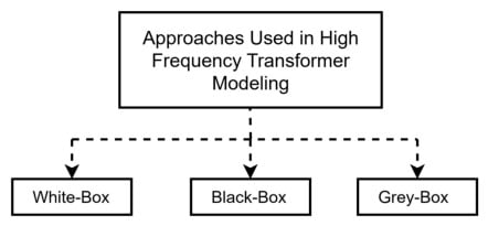
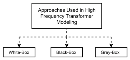
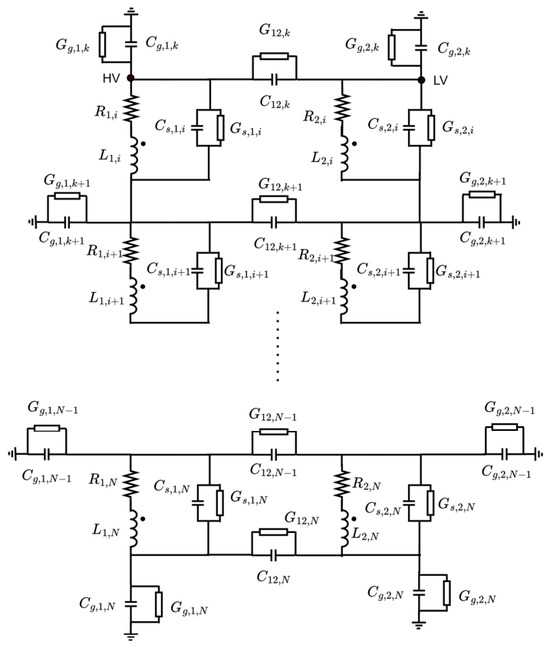
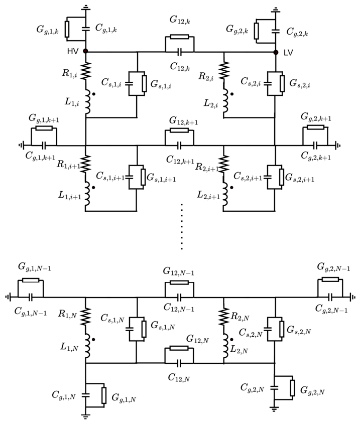
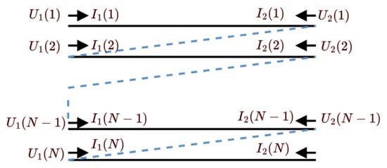
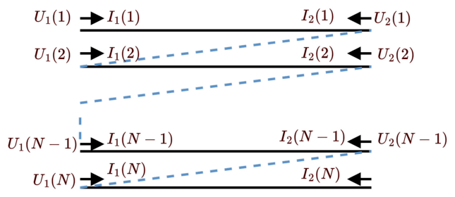
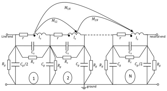
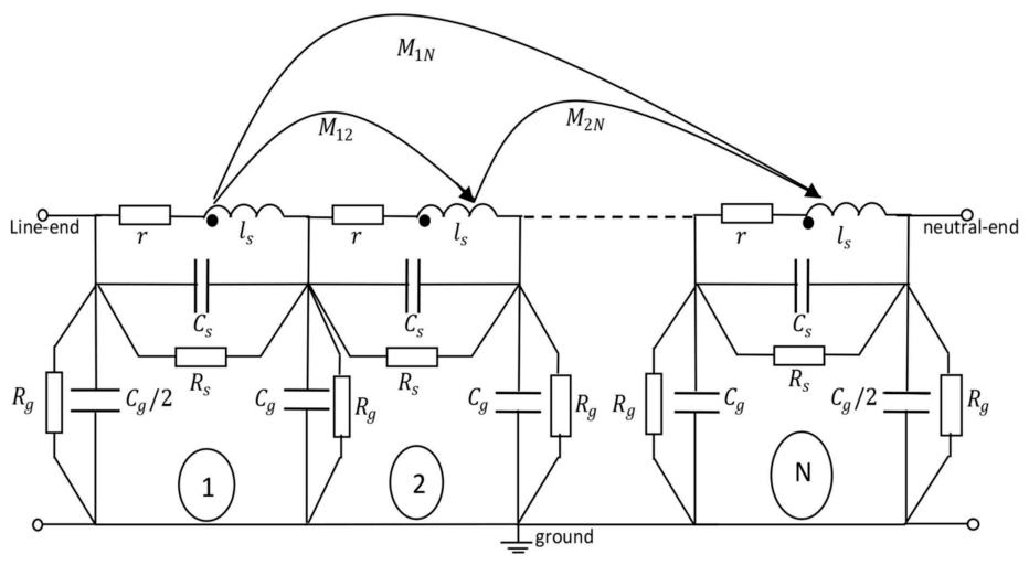
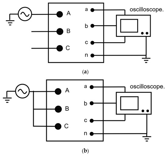
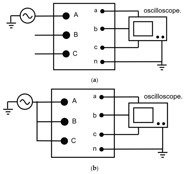
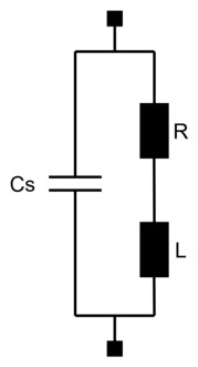
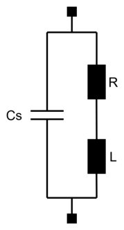
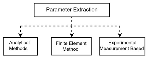
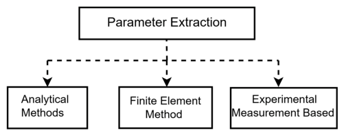
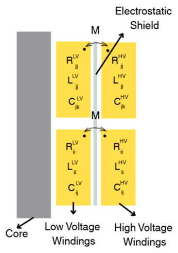
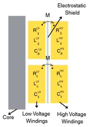
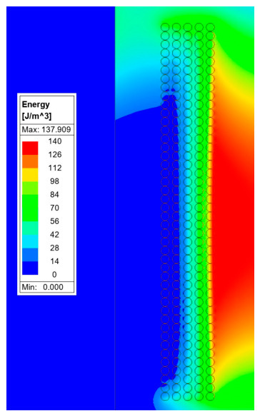
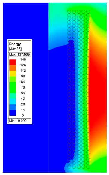
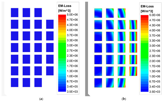
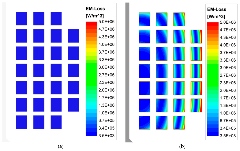
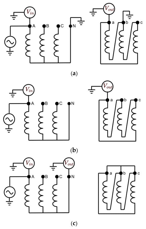
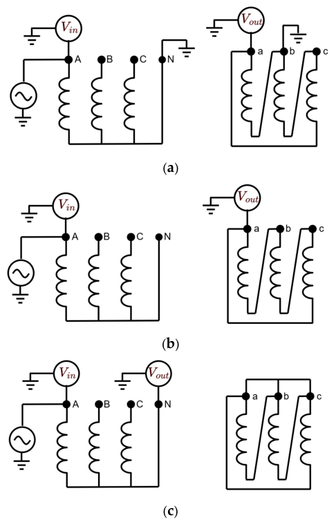
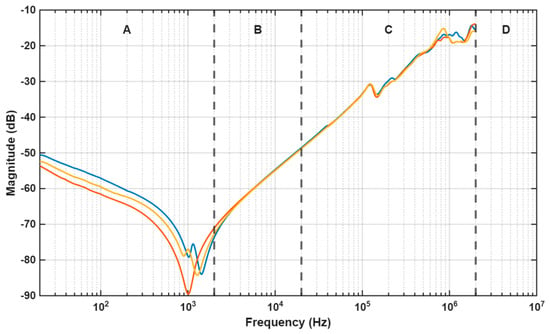
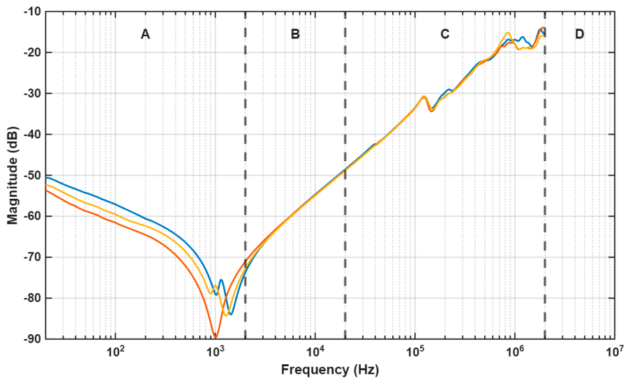
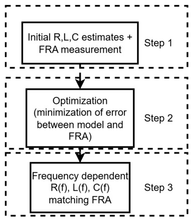
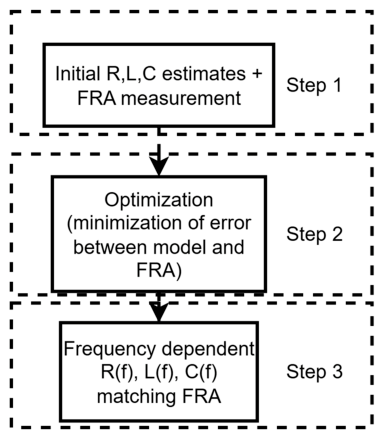
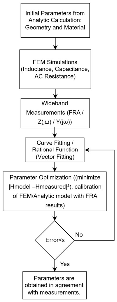
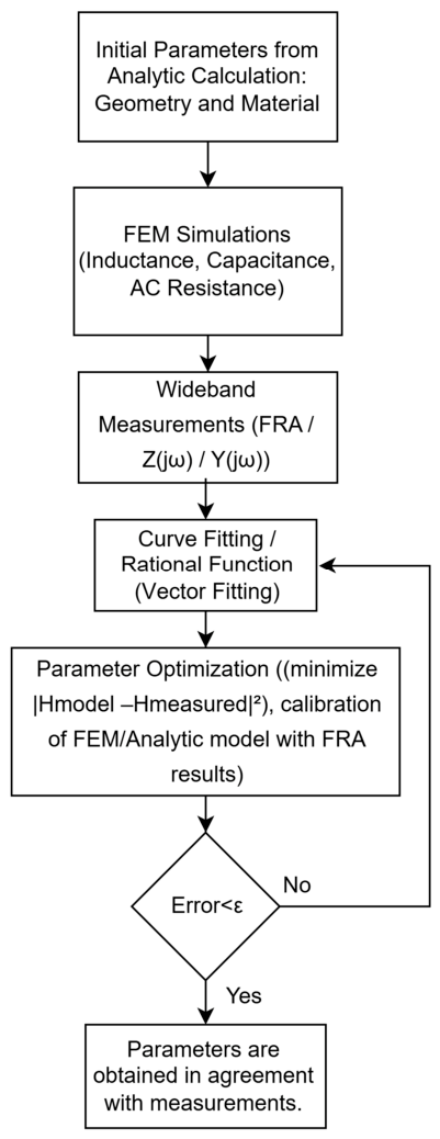



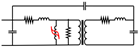
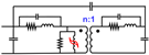
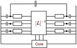
Disclaimer/Publisher’s Note: The statements, opinions and data contained in all publications are solely those of the individual author(s) and contributor(s) and not of MDPI and/or the editor(s). MDPI and/or the editor(s) disclaim responsibility for any injury to people or property resulting from any ideas, methods, instructions or products referred to in the content. |
© 2026 by the authors. Licensee MDPI, Basel, Switzerland. This article is an open access article distributed under the terms and conditions of the Creative Commons Attribution (CC BY) license.