


Abstract
Maintenance scheduling in large run-of-river hydropower plants requires balancing maintenance urgency, asset condition, hydrological opportunity, and operational constraints. This study proposes an integrated decision-support framework for the Santo Antônio Hydropower Plant, a 50-unit facility in Brazil. The methodology combines condition-informed maintenance inputs, multi-criteria prioritization of generating-unit maintenance needs, and a Forced Impact of Downtime (FID)-guided Large Neighborhood Search (LNS) algorithm with problem-specific destroy-and-repair operators. The optimization reallocates eligible maintenance activities from high-impact hydrological periods while enforcing resource, electrical, hydraulic, and synchronization constraints. The proposed approach was compared with Genetic Algorithm (GA) and Ant Colony Optimization (ACO) benchmarks over 1000 independent runs using real operational data. LNS achieved the lowest mean fitness value (3587.68), compared with 3939.45 for ACO and 3964.54 for GA, and the shortest average execution time. Relative to the baseline schedule prepared by plant specialists, the optimized schedule reduced FID from 452 to 302 equivalent unavailability hours, corresponding to a 33.2% reduction. These results demonstrate the potential of hydrology-aware, condition-informed optimization to support practical maintenance planning in large run-of-river hydropower plants.
1. Introduction
Maintenance scheduling is a critical task in the operation of large-scale hydropower plants, since planned outages directly affect generation availability, equipment reliability, and operational risk [1,2]. In plants composed of dozens of generating units, maintenance decisions must account not only for the technical need to intervene in specific assets, but also for the hydrological period in which each unit is removed from service. This coupling between maintenance requirements and water availability makes hydropower maintenance planning a complex decision-making problem.
In run-of-river hydropower plants, the operational impact of a planned outage depends strongly on the inflow condition. Removing a generating unit from service during periods of high hydrological availability may increase spillage or reduce the plant’s ability to convert the available flow into electrical energy. Conversely, the same intervention may have lower operational impact when scheduled during periods of reduced water availability. Therefore, maintenance scheduling should not be treated as a purely calendar-based allocation problem. It requires a coordinated evaluation of outage timing, unit availability, maintenance duration, hydrological opportunity, and operational restrictions.
However, optimizing only the hydrological convenience of outages may also lead to inadequate decisions. Some maintenance activities are associated with component degradation, safety exposure, forced-outage risk, or recurrent technical issues. Delaying these interventions only because they are inconvenient from an availability perspective may increase asset risk and compromise maintenance governance. Thus, a practical scheduling framework must simultaneously consider two complementary aspects: the operational cost of stopping a unit and the technical urgency of performing each maintenance activity.
This paper addresses this challenge in the context of the Santo Antônio Hydropower Plant, a large run-of-river facility composed of 50 generating units. The scheduling problem involves several maintenance classes, different execution durations, unit-level restrictions, shared resources, overhead-crane (portico) constraints, electrical subsystem limits, hydraulic-level requirements, and group synchronization rules. In addition, some maintenance requests are derived from asset-condition information, such as condition-based recommendations for phenolic gasket replacement. In this work, such condition-based recommendations are treated as scheduling inputs to be prioritized and allocated together with the remaining planned maintenance activities.
To support this decision-making process, this work proposes an integrated maintenance scheduling framework that combines condition-based maintenance inputs, multi-criteria prioritization, and metaheuristic optimization. The condition-based input layer converts degradation-driven maintenance needs into structured scheduling requests. The prioritization module transforms heterogeneous maintenance indicators into comparable urgency scores by combining local generating-unit condition with maintenance-class criticality. The optimization module then constructs feasible schedules using a Forced Impact of Downtime (FID)-guided Large Neighborhood Search (LNS) algorithm.
The use of LNS is motivated by the combinatorial structure of the problem. A maintenance schedule can be represented as a set of generating-unit–maintenance pairs associated with start and end dates. Small changes in these dates may affect feasibility, overlap, hydrological impact, and priority-related penalties. Exact optimization approaches may become computationally expensive when applied to realistic instances with many units, maintenance types, and operational constraints. The computational complexity of large-scale maintenance scheduling has motivated the adoption of heuristic and metaheuristic optimization techniques in practical power-system applications [1,3,4]. A preliminary version of the optimization framework was presented in [5], where GA, ACO, and LNS were compared for the maintenance-scheduling problem using a common FID-based evaluation framework. The present journal article substantially extends that conference study in both methodological scope and experimental validation. Specifically, the previous work focused primarily on the comparative performance of the three metaheuristics, whereas the present study (i) formalizes a condition-based maintenance input layer that converts degradation forecasts into structured maintenance requests; (ii) formalizes and expands a detailed multi-criteria prioritization model that combines unit-level condition indicators with maintenance-class criticality; (iii) reformulates the scheduling objective to explicitly integrate hydrological impact, priority consistency, seasonal allocation preferences, and end-of-horizon penalties; (iv) provides a more detailed mathematical representation of the plant-specific operational constraints and of the FID-guided LNS operators; and (v) expands the experimental assessment from 100 to 1000 independent executions per method and includes a direct schedule-level comparison with the maintenance plan prepared by plant specialists. Therefore, the present work should be regarded as a substantial methodological and experimental extension of the preliminary conference study rather than a repetition of the previously reported benchmark.
In the proposed implementation, the destroy operator is guided by the daily FID contribution of the current schedule. Eligible non-protected activities allocated in high-impact periods are selected for removal, and the repair operator attempts to reinsert them into lower-impact feasible dates while respecting hard operational constraints. This strategy directly exploits the hydrological structure of the objective function, making the search process more informed than purely random perturbation mechanisms.
The main contributions of this paper are summarized as follows:
- A formalized end-to-end decision-support framework that connects condition-based maintenance recommendations, maintenance prioritization, and hydrology-aware scheduling within a single computational workflow.
- A condition-based input layer that transforms degradation-derived recommendations into structured maintenance requests that can be directly incorporated into the scheduling problem.
- A multi-criteria prioritization methodology that combines maintenance-specific unit condition indicators with the global criticality of each maintenance class, producing a unified priority score for each generating-unit–maintenance pair.
- An extended scheduling formulation in which the FID-based hydrological criterion is combined with priority consistency, seasonal allocation preferences, end-of-horizon penalties, and a detailed representation of plant-specific hard operational constraints.
- An expanded computational and operational validation based on 1000 independent executions of each metaheuristic and a direct comparison between the optimized schedule and the original maintenance plan developed by plant specialists.
The results show that the proposed LNS method outperformed the benchmark approaches in solution quality and computational time. The obtained results are consistent with the literature, which reports that neighborhood-search-based optimization techniques are particularly effective for large-scale maintenance scheduling problems with complex operational constraints [3,6]. In the evaluated benchmark campaign, LNS achieved the lowest mean fitness value, the best individual solution, and the shortest average execution time. At the schedule level, the optimized plan reduced FID from 452 to 302 equivalent unavailability hours, corresponding to an approximate reduction of 33.2%. These results indicate that the proposed framework can produce feasible, interpretable, and hydrologically efficient maintenance schedules while preserving the priority of technically critical interventions.
The remainder of this paper is organized as follows. Related Work Section presents the literature review. Section 2 describes the maintenance scheduling problem at the Santo Antônio Hydropower Plant, highlighting the operational characteristics of the plant, the hydrological seasonality of the Madeira River, and the main planning challenges associated with generating-unit outages. Section 3 presents the proposed methodology, including the condition-based maintenance inputs, prioritization, and optimization modules. Section 4 reports the computational results, benchmark comparison, and schedule-level analysis. Finally, Section 5 concludes the paper and discusses future research directions.
Related Work
Maintenance scheduling in power systems has been extensively studied due to its direct influence on generation availability, reliability, operating costs, and asset-management decisions. In the electricity industry, maintenance planning typically involves the allocation of preventive or condition-driven outages over a finite horizon while satisfying technical, operational, reliability, and resource constraints. Comprehensive reviews show that this problem appears in different forms across regulated and deregulated power systems, including generator maintenance scheduling, transmission maintenance, integrated generation–transmission maintenance, and maintenance planning under uncertainty [1,7].
Generator maintenance scheduling (GMS) is one of the most established formulations in this field. In classical GMS models, the decision maker determines the periods in which generating units should be removed from service while preserving system adequacy and minimizing cost, risk, or reliability-related indicators. Mathematical programming formulations provide rigorous modeling structures for this class of problems, especially when unit availability, maintenance duration, continuity, and operational limits must be explicitly represented. However, realistic instances may become computationally demanding due to the large number of binary variables and coupling constraints, particularly when high temporal resolution, hydropower allocation, or long planning horizons are considered [1,8,9].
To overcome the computational limitations of exact approaches, several studies have applied heuristic and metaheuristic techniques to maintenance scheduling. Dahal and Chakpitak [10] investigated genetic algorithms, simulated annealing, and hybrid strategies for generator maintenance scheduling, showing the ability of metaheuristics to explore large constrained search spaces. Other works have proposed thermal generator scheduling procedures based on metaheuristic search [11], differential evolution assisted by mathematical programming structures [12], and exchange market algorithms for GMS [13]. More recently, multi-objective formulations have been proposed to represent conflicting maintenance objectives such as cost, reliability, and violation minimization [3]. These studies support the use of metaheuristics when exact optimization becomes difficult or when multiple practical criteria must be incorporated.
The broader power and energy systems literature also emphasizes the importance of careful benchmark design when using metaheuristics. Chicco and Mazza [14] discuss the risks of applying generic metaheuristics without sufficient customization, highlighting the need for problem-specific operators and fair comparisons. This observation is particularly relevant for maintenance scheduling, since feasibility is often governed by highly specific operational constraints, such as resource limits, equipment dependencies, electrical restrictions, hydraulic windows, and temporal synchronization requirements. Real-world energy management and power-grid maintenance applications further illustrate that scalable heuristic or matheuristic approaches are frequently required when industrial constraints make exact solution methods impractical [15,16].
Large Neighborhood Search (LNS) is especially suitable for highly constrained scheduling problems because it modifies a solution by partially destroying and reconstructing selected components. The method was originally introduced in the context of vehicle routing in [17] and later systematized as a general metaheuristic framework by Pisinger and Ropke [18]. Its adaptive variant, ALNS, further improves the search by dynamically selecting destroy and repair operators according to their historical performance [19]. In maintenance scheduling applications, Woller and Kulich [6] demonstrated the suitability of ALNS for handling complex feasibility structures through iterative removal and insertion procedures. These characteristics motivate the use of an LNS-based approach in the present work, where maintenance activities must be reallocated without violating hard operational constraints.
In hydropower plants, maintenance scheduling introduces additional challenges compared with thermal or generic generation benchmarks. Planned outages interact with inflow seasonality, hydraulic availability, turbine-flow capacity, shared plant infrastructure, and operational restrictions imposed by electrical and hydraulic systems. In run-of-river plants, the impact of removing a generating unit from service may vary substantially depending on the hydrological period in which the outage is scheduled. Consequently, a maintenance plan that is feasible from a resource-allocation perspective may still be inefficient if high-priority outages are concentrated in periods of high hydrological opportunity.
Post-maintenance return-to-service procedures also introduce technical requirements that must be considered in hydropower maintenance planning. Transient operating conditions associated with start-up, shutdown, load rejection, and other operating transitions may produce significant hydraulic and mechanical effects. Recent work has investigated physics-based and data-aided prediction of transient behavior in pumped-storage hydropower systems [20], while experimental studies have characterized transient pressure behavior during emergency shutdown, total load rejection, and runaway conditions in hydraulic turbines [21]. Although these studies address turbine configurations and transient-analysis objectives that differ from the run-of-river scheduling problem considered here, they highlight the importance of post-maintenance commissioning and safe return-to-service procedures. The present work does not simulate transient hydraulic dynamics explicitly; instead, their operational implications are represented through maintenance-specific testing and commissioning periods included in the scheduling model.
Another important aspect is that maintenance activities are not homogeneous. Different intervention classes may involve different operational consequences, degradation relevance, safety implications, and planning urgency. Recent studies in condition-based and risk-informed maintenance emphasize that maintenance decisions should consider equipment condition, operational criticality, and production impact instead of relying exclusively on fixed preventive intervals [22,23]. Therefore, practical maintenance scheduling frameworks must be able to incorporate condition-based maintenance requests and priority information while still respecting hydrological and operational constraints.
Recent inspection and maintenance optimization studies further reinforce the importance of coupling asset-condition information with maintenance-timing decisions. Li et al. [24] proposed a group inspection and maintenance policy for heterogeneous multi-component systems that explicitly considers component-specific degradation behavior, maintenance requirements, and shared maintenance resources. Wei et al. [25] developed a predictive inspection and maintenance policy based on the belief-based semi-Markov decision process, allowing for inspection and maintenance decisions to be made at non-equidistant time intervals according to the estimated system condition. These studies focus primarily on inspection and maintenance policy design, whereas the present work addresses the subsequent plant-level scheduling problem, in which condition-derived maintenance recommendations must be coordinated with hydrological opportunity and operational constraints.
Despite these advances, few studies integrate condition-based maintenance inputs, multi-criteria prioritization, hydrological opportunity, and LNS-based optimization into a single scheduling framework for large run-of-river hydropower plants. Most GMS studies focus on thermal units or general power-system benchmarks, while large hydropower plants require additional modeling of inflow seasonality, unit hydraulic availability, shared infrastructure, electrical restrictions, and the operational impact of planned generating-unit outages.
This work addresses this gap by proposing an integrated decision-support framework for the maintenance scheduling of 50 generating units at the Santo Antônio Hydropower Plant. The proposed methodology combines condition-based maintenance inputs, multi-criteria prioritization of generating-unit–maintenance pairs, and a Forced Impact of Downtime (FID)-guided LNS algorithm. By explicitly linking maintenance urgency, hydrological impact, and hard operational constraints, the proposed approach contributes both to the maintenance scheduling literature and to practical planning in large run-of-river hydropower plants.
2. Maintenance Scheduling Problem at Santo Antônio Hydropower Plant
The Santo Antônio Hydropower Plant (SAE) plays a fundamental role in the Brazilian electrical energy system, with an installed capacity of approximately 3568 MW, as reported in [26]. It is currently one of the largest hydropower plants in Brazil, ranking among the top five in terms of installed capacity.
The plant is located on the Madeira River and operates as a run-of-river facility. This characteristic imposes significant operational challenges due to the high seasonal variability of river inflows. In particular, the Madeira River exhibits substantial hydrological fluctuations throughout the year, with high flow rates typically observed during the Brazilian summer (early months of the year) and significantly reduced flows during the dry season, especially between June and September.
These hydrological conditions have a direct impact on the operation of generating units (GUs), as periods of low inflow often lead to hydraulic constraints that limit power generation or even force unit shutdowns. Consequently, maintenance scheduling must be carefully aligned with these seasonal patterns in order to take advantage of periods in which unit unavailability is unavoidable due to reduced water availability.
Therefore, the maintenance scheduling problem at SAE consists of determining an optimal allocation of maintenance activities over time, considering both operational constraints and hydrological conditions. The objective is to strategically assign maintenance outages to periods of lower water availability, thereby minimizing the impact on energy production.
At the same time, the scheduling process must ensure equipment reliability and compliance with maintenance requirements, while minimizing key performance indicators such as total unavailability hours and the Forced Impact of Downtime (FID). This results in a highly constrained and large-scale optimization problem, requiring advanced solution techniques to obtain high-quality schedules.
3. Methodology
This section describes the proposed decision-support framework for maintenance scheduling in a large run-of-river hydropower plant. The methodology integrates three computational layers: (i) a condition-based input layer, which converts degradation-driven maintenance needs into structured maintenance requests; (ii) a multi-criteria prioritization module, which ranks maintenance needs according to operational, degradation, and planning criteria; and (iii) an optimization module, which constructs and improves feasible maintenance schedules using Large Neighborhood Search (LNS), while also allowing for benchmarking against Genetic Algorithm (GA) and Ant Colony Optimization (ACO) implementations.
Unlike a purely calendar-based planning procedure, the proposed framework couples asset condition indicators, hydrological availability, unit-level operational constraints, and maintenance priorities within a unified optimization workflow. Figure 1 summarizes the end-to-end architecture adopted in this work.
Figure 1.
Proposed integrated methodology for condition-informed, priority-driven and hydrology-aware maintenance scheduling.
3.1. Condition-Based Maintenance Input
Some maintenance activities considered in the scheduling problem are not defined exclusively by fixed calendar intervals. In particular, VE maintenance, associated with phenolic gasket replacement, depends on the degradation condition observed during periodic inspections. Therefore, before the optimization stage, inspection records are converted into condition-based maintenance recommendations that can be incorporated into the maintenance planning process.
In this work, the VE replacement horizon is obtained from a degradation-forecasting procedure that combines data-driven time-series prediction with probabilistic degradation assessment. Historical measurements of the upper and lower phenolic gasket regions are used to estimate a candidate replacement horizon, while a Weibull-based Monte Carlo assessment is applied to verify whether the recommended date is consistent with the adopted replacement-probability threshold. The detailed development and validation of the degradation model are outside the main scope of this scheduling-oriented study; here, this degradation-forecasting procedure is used only as an input-generation layer for the optimizer.
From the perspective of the proposed maintenance scheduling framework, the output of this stage is a set of VE maintenance requests. Each request identifies the generating unit, the maintenance class, and the recommended replacement date. In compact form, the condition-based VE recommendation for generating unit u is represented as
where denotes the recommended replacement date obtained from the degradation-forecasting procedure.
These VE recommendations are then combined with the remaining planned maintenance activities and forwarded to the prioritization and optimization modules. For VE maintenance, the condition-based module provides a recommended replacement date, which is used by the optimizer as the preferred execution date. The scheduling procedure first attempts to allocate the activity on this date. If the proposed allocation violates any hard operational or scheduling constraint, the maintenance is reassigned to the closest feasible date. Therefore, the predicted VE date is not treated as an unconditional fixed date, but as a preferred scheduling reference whose final allocation remains subject to operational feasibility. Other maintenance classes are not driven by this predictive module and follow their respective prioritization criteria based on generating-unit operational parameters.
3.2. Multi-Criteria Prioritization Module
The prioritization module converts heterogeneous maintenance information into a unified score that represents the relative urgency of each generating-unit–maintenance pair. This step is necessary because maintenance scheduling cannot be guided only by operational availability indicators, such as the Forced Impact of Downtime (FID), accumulated unavailability hours, or hydrological opportunity. Although these quantities are essential to estimate the operational cost of removing a unit from service, they do not fully capture the risk associated with postponing critical interventions. In some cases, delaying a maintenance activity may increase the probability of asset degradation, forced outages, safety hazards, or collateral damage to auxiliary systems.
The proposed framework separates the notion of when it is convenient to stop a unit from the notion of which maintenance actions are more critical. The first aspect is mainly addressed by the optimization module through FID and scheduling constraints, whereas the second is addressed by the prioritization module. The output of this module is a ranked list of candidate maintenance activities, in which each element is associated with a generating unit, a maintenance type, and a global priority score.
The prioritization pipeline is composed of three main stages, as illustrated in Figure 2. Let denote the set of generating units and the set of maintenance types considered in the planning problem. Each candidate maintenance requirement is therefore represented by a pair , where identifies the generating unit and denotes the corresponding maintenance activity.
Figure 2.
Multi-criteria prioritization workflow.
The objective of the prioritization module is to assign a unified priority score to every candidate pair . To achieve this, the procedure is divided into three sequential stages. First, the generating units are ranked independently for each maintenance type according to maintenance-specific condition indicators. Second, each maintenance type is assigned a global criticality score based on four planning criteria: impact on FID, rescheduling relevance, required maintenance resources, and degradation condition. Finally, the local ranking of each generating unit is combined with the global maintenance criticality score, producing a single priority score that quantifies the overall importance of scheduling maintenance type m on generating unit u.
For every pair , the available information is organized into a condition vector , whose composition depends on the maintenance type under analysis. This vector may include physical measurements, inspection results, elapsed time since the last intervention, binary execution indicators, leakage levels, crack severity, transformer-related variables, adjustment-ring condition, or other maintenance-specific descriptors. Since different maintenance classes rely on distinct technical indicators, the local condition score is computed through a maintenance-dependent scoring function:
where denotes the scoring rule associated with maintenance type m, mapping the available condition indicators into a normalized priority score. Consequently, represents the lowest maintenance priority within that maintenance class, whereas identifies the generating unit with the highest urgency according to the adopted criterion.
The value represents the relative priority of generating unit u within the candidate list of maintenance type m. A score close to zero indicates low urgency for that specific maintenance action, while a score close to one indicates that the unit is among the most critical candidates for that maintenance type. This normalization is important because the original indicators may have different units and scales, such as days, millimeters, qualitative inspection classes, or binary conditions.
Table 1 summarizes the main rule families used to build the unit-level rankings. The objective is not to impose a single scoring model for all maintenance types, but to preserve the physical interpretation of each maintenance indicator while mapping all outputs to a common priority scale.
Table 1.
Examples of local scoring rules used to rank generating units within each maintenance type.
After the unit-level ranking is obtained for each maintenance type, the module evaluates the global criticality of the maintenance class itself. This second stage is required because two maintenance types may produce similar local scores but represent different operational consequences. For example, a high local score in a low-impact preventive activity may be less urgent than a moderate local score in a maintenance class associated with safety, severe degradation, or high forced-outage risk.
The global maintenance criticality score is computed from a set of prioritization criteria . Each criterion c has an importance weight , while the maintenance type m receives two normalized assessments under that criterion: a probability-related component and an impact-related component . The resulting score is defined as
In this formulation, the product emphasizes maintenance types that simultaneously present high likelihood and high consequence under a given criterion. The weight allows for the decision maker to adjust the relative importance of the different planning dimensions.
For the case study considered in this work, four criteria were adopted in the global maintenance-class assessment: impact on FID, rescheduling relevance, required maintenance resources, and degradation condition. Their nominal weights were set to 0.20, 0.10, 0.10, and 0.60, respectively, as summarized in Table 2. The weights sum to one and define the reference prioritization configuration used throughout the case study.
Table 2.
Criteria and nominal weights adopted in the global maintenance-class prioritization for the case study.
The influence of these expert-defined weights is examined through the sensitivity analysis presented in Section 4.5.
The local and global dimensions are then combined into a single priority score for each unit–maintenance pair. The score assigned to pair is given by
This definition preserves the internal ranking of generating units for the same maintenance type while also accounting for the relative importance of different maintenance classes. As a consequence, a unit with a high local urgency in a highly critical maintenance type receives a high global score, whereas a similar local score in a less critical maintenance class receives a lower global priority.
The final output of the prioritization module is the ordered set
where the sorting operation ranks the candidate pairs in decreasing order of . This list can be filtered by execution limits defined for each maintenance type. If denotes the maximum number of activities of type m to be forwarded to the optimizer, the selected candidate set is
This filtering step reduces the size of the scheduling problem and avoids allocating optimization effort to low-priority interventions that are not expected to be executed within the considered planning cycle. At the same time, it preserves the most critical maintenance needs identified for each maintenance class.
The selected set is then converted into structured maintenance requests and passed to the optimization module. In the following stages, the global priority score is also used as part of the fitness-function penalization mechanism. Thus, schedules that postpone or poorly allocate high-priority maintenance activities are penalized more strongly than schedules that delay low-priority interventions. The complete mathematical definition of this priority-dependent penalty is presented in the fitness-function formulation.
3.3. Optimization Module
The optimization module is the final computational layer of the proposed methodology. It receives the maintenance requests generated by the condition-based input and prioritization modules and transforms them into an executable maintenance schedule for the hydropower plant. In this stage, each candidate schedule is evaluated according to hydrological opportunity, operational restrictions, maintenance priority, and calendar feasibility.
The optimization problem is not limited to minimizing the number of unavailable units or distributing outages uniformly over time. In a run-of-river hydropower plant, the operational impact of stopping a generating unit depends strongly on the available flow, hydraulic head, turbine class, and the number of units already unavailable on the same day. Therefore, the optimizer must decide not only which maintenance actions will be executed, but also when each action should start so that high-priority interventions are allocated with minimum operational impact.
Figure 3 summarizes the main steps of the optimization module. The candidate maintenance set is first encoded as a schedule, then evaluated through the hydrological model and the constraint-checking procedures. The resulting feasible schedules are compared using the fitness function. The proposed Large Neighborhood Search (LNS) algorithm improves the schedule iteratively, while Genetic Algorithm (GA) and Ant Colony Optimization (ACO) implementations are used as benchmark methods.
Figure 3.
Optimization module workflow.
3.3.1. Problem Definition and Solution Encoding
In the implemented optimization model, a maintenance activity is structured according to the same information required by the scheduling system: generating unit, maintenance type, start day, and end day. Thus, the basic scheduling object associated with activity j is represented as
The first two elements, and , identify the generating unit and the maintenance type. These values are fixed once the candidate maintenance set is defined by the previous modules. The start day is the decision variable adjusted by the optimizer, while the end day is calculated from the start day and the effective duration of the corresponding maintenance activity. Therefore, the optimizer manipulates dates, but the schedule itself remains directly interpretable by maintenance planners.
A complete maintenance schedule is a list of activities of the form given in (7). This list represents both the output expected by the maintenance planning process and a candidate solution of the optimization problem:
A maintenance schedule can also be represented by its decision variables, namely the planned start day of each maintenance activity. Let
denote the scheduled start day of maintenance activity j, where is the set of admissible start dates determined by technical, operational, and planning constraints. Since the activity duration is fixed once the maintenance type is defined, the end date is implicitly obtained from the corresponding execution time.
Using this notation, an entire maintenance schedule is encoded by the start-date vector
where each component specifies the planned starting day of one maintenance activity. This representation is particularly convenient for metaheuristic optimization because neighborhood operators only need to modify selected start dates while preserving the corresponding generating unit and maintenance type. Consequently, destroy-and-repair operators can explore different temporal allocations without altering the composition of the maintenance plan itself.
The end day of each activity is a deterministic consequence of its start day. In addition to the nominal maintenance duration, most interventions require on-site commissioning tests before the generating unit can return to normal operation. Depending on the maintenance class, the commissioning stage typically adds either two or four days to the activity duration. These commissioning days are explicitly included in the scheduling interval and therefore affect generating-unit availability, operational-constraint checking, and the FID calculation. Additional technical stages may also include drying, draining, and refilling, while calendar effects such as weekends and non-working days may further modify the effective duration. The detailed transient phenomena and commissioning test procedures themselves are outside the scope of the present scheduling study. For activity j, this duration is modeled as
combining the nominal execution time , the additional technical time required by maintenance type , and the calendar correction . Once is known, the corresponding end day is obtained by
Let denote the reference planning horizon, with days in the case study considered in this work. Maintenance start dates are restricted to this reference horizon. However, an activity starting within may extend beyond day T because of its effective duration. Therefore, denotes the extended calendar used to represent complete activity intervals and to verify feasibility after the end of the reference horizon. Hydrological impact and FID are evaluated over , whereas unit unavailability occurring in is accounted for through the end-of-horizon penalty.
Each maintenance activity occupies the calendar interval:
Given a candidate schedule , the daily unavailability state of each generating unit is derived from the activity intervals. The binary variable indicates whether unit u is unavailable on day t due to at least one scheduled activity:
This variable links the activity-level schedule to the hydrological and operational evaluations. Once is known for all units and days, the optimizer can compute the number of unavailable units by turbine class, identify operational conflicts, estimate the Forced Impact of Downtime (FID), and evaluate the fitness function.
Using this representation, the scheduling problem can be written in compact form as
with representing the feasible schedules and the fitness function used to compare candidate solutions. The feasible set is defined by the operational, hydraulic, electrical, logistical, and calendar constraints described in Section 3.3.4. The LNS algorithm explores this space by partially destroying and repairing the activity list, always preserving the interpretation of a solution as a maintenance schedule composed of generating-unit, maintenance-type, start-day, and end-day records.
3.3.2. Hydrological Evaluation and Forced Impact of Downtime Calculation
The hydrological evaluation estimates the operational impact caused by the maintenance outages contained in a candidate schedule. This step is essential because the same maintenance activity may have different consequences depending on the flow available on the scheduled day. Stopping a unit during a low-flow period may have negligible impact, whereas the same outage during a high-flow period may increase spilled water or reduce the ability of the plant to convert the available hydrological resource into electricity.
The principal variables employed throughout the hydrological evaluation are summarized in Table 3. These symbols are consistently used in the equations that model turbine availability, hydraulic capacity, spilled-flow estimation, and the Forced Impact of Downtime (FID).
Table 3.
Main variables used in the hydrological evaluation.
For each day t, the evaluator uses the daily long-term mean (MLT) river-flow series , the upstream level , and a downstream-level curve . The net head considered in the turbine performance calculation is given by
where is an empirical hydraulic adjustment associated with the operating condition. The resulting head is used to evaluate turbine performance curves for the two turbine classes present in the plant, namely four-blade and five-blade units. These classes are represented by the set .
For turbine class b, the turbine discharge of one available unit on day t is denoted by . The number of units of class b effectively available under schedule x is computed after removing the units unavailable due to planned maintenance:
Here, represents the number of hydraulically available units of class b before maintenance scheduling effects, and is the subset of generating units belonging to class b.
The total turbine-flow capacity available under the candidate schedule is then
The average turbine flow of the available units is used to translate spilled flow into equivalent unavailable-unit time. It is calculated as
The available river flow is adjusted by the flow deviations associated with the fish transposition system and the log spillway system, denoted by and , respectively. The required number of units to absorb this adjusted flow is approximated by
Although is not directly included as a separate penalty term in the objective function, it provides an auxiliary hydrological indicator for interpreting the relationship between the available turbine capacity and the flow absorption requirement under a given maintenance schedule.
The main hydrological penalty is derived from a spilled-flow proxy. Let be the turbine capacity that would be available if all hydraulically available units were not under planned maintenance. The additional flow that cannot be absorbed because of the scheduled outages is estimated by
The daily contribution to the Forced Impact of Downtime is obtained by converting this flow deficit into equivalent unit-hours of forced impact:
The total FID associated with schedule x is accumulated over the reference planning horizon:
Since () and () are both expressed as flow rates, the ratio () represents the equivalent number of generating units affected by the flow deficit. Multiplication by 24 converts this quantity into equivalent generating-unit hours, while division by () expresses the result as average equivalent unavailability hours per generating unit. Therefore, () and () are expressed in hours on a plant-normalized basis.
From an engineering perspective, FID should be interpreted as a measure of lost hydrological utilization opportunity caused by scheduled unit unavailability. When the available river flow exceeds the turbine-flow capacity of the generating units remaining in service, the excess-flow term represents water that cannot be processed by the available turbines under the considered operating condition. Therefore, a larger FID indicates that maintenance outages coincide more strongly with periods in which additional turbine capacity would otherwise be useful for absorbing the available flow.
FID is not, however, a direct measurement of electrical energy loss in MWh. Its formulation converts the unabsorbed-flow proxy into equivalent generating-unit hours and normalizes it at plant level. A direct conversion to lost electrical energy would additionally require the integration of unit-specific power-output and efficiency characteristics over time. Accordingly, FID is used in this work as an operational proxy for the generation opportunity affected by maintenance outages: reducing FID indicates a lower exposure of scheduled unavailability to periods with potentially relevant spill or generation loss, but should not be interpreted as an equivalent numerical reduction in MWh.
This metric penalizes schedules that remove generating units from operation on days when the remaining turbine capacity is insufficient to absorb the available flow. Consequently, the optimizer is encouraged to allocate outages to periods with lower hydrological opportunity or lower marginal impact on plant availability.
3.3.3. Fitness Function
The fitness function compares candidate schedules by combining hydrological impact, maintenance-priority consistency, seasonal allocation preferences, and end-of-horizon extensions. Since the original components represent different planning quantities, the penalty terms are reformulated on a common temporal scale before aggregation. The FID term is already expressed as average equivalent unavailability hours per generating unit. The remaining components are converted into hour-based measures and normalized according to their respective aggregation structures.
The objective minimized by the optimizer is defined as
where (), (), (), and () are dimensionless preference coefficients. The superscript () indicates that the corresponding penalty has been converted to an hour-based temporal measure.
The priority component discourages schedules in which high-priority maintenance activities are allocated later than lower-priority activities. The total pairwise priority weight is first defined as
The hour-based priority penalty is then expressed as
In these expressions, represents the total weighted temporal inversion among maintenance activities, whereas is the corresponding total pairwise priority weight. The normalization by prevents the priority component from increasing merely because the number of pairwise comparisons increases. Consequently, represents the weighted average temporal inversion of the maintenance priorities, expressed in hours. The term is zero when every higher-priority activity starts no later than each lower-priority activity against which it is compared.
The seasonal component represents the undesired allocation of five-blade generating-unit outages during the dry period. Since the original summation is expressed in generating-unit days, it is converted to hours and normalized by the total number of generating units:
Here, denotes the set of dry-season days, defined in this study as the period from June through September, and denotes the set of five-blade generating units.
Therefore, () represents the average equivalent unavailability hours per plant generating unit associated with discouraged five-blade-unit outages during the dry period. The normalization by () is consistent with the plant-level normalization adopted in the FID calculation.
To avoid counting multiple simultaneous maintenance activities on the same generating unit more than once, the end-of-horizon component is defined from the unit-level unavailability state rather than from the individual activity overruns. Let
denote the set of calendar days contained in the extended calendar but located after the reference planning horizon. The end-of-horizon penalty is defined as
This term represents the average equivalent unavailability hours per generating unit occurring after the reference planning horizon. Unlike an activity-based overrun summation, this formulation counts each unavailable generating unit only once per day, even when multiple compatible maintenance activities are executed simultaneously on the same unit.
Accordingly, all four objective components are represented on an hour-based temporal scale. However, they retain distinct operational interpretations: () measures hydrologically induced equivalent unavailability, () measures the weighted average time associated with priority inversions, () measures discouraged dry-period unavailability, and () measures unavailability extending beyond the reference horizon. The preference coefficients in (24) therefore control the trade-off among these planning dimensions rather than performing unit conversions.
3.3.4. Operational Constraints
The optimizer enforces operational restrictions during schedule construction and repair. Candidate insertions that violate hard constraints are rejected before fitness evaluation, which reduces the number of infeasible solutions explored by the metaheuristic. These restrictions represent practical limitations related to maintenance crews, shared equipment, electrical reliability, hydraulic conditions, and execution continuity.
Commissioning periods are treated as part of the corresponding maintenance execution intervals. Consequently, the applicable crew and execution-capacity limits, calendar restrictions, weekend-related rules, and other operational constraints remain active when these post-maintenance stages are scheduled.
The first group of constraints is associated with the temporal feasibility of activity starts. Every scheduled start day must belong to its admissible set. The end of an activity may exceed the reference planning horizon, but such extensions are penalized through in the fitness function:
Maintenance activities on the same generating unit are not allowed to overlap unless the corresponding maintenance types are explicitly configured as compatible for parallel execution. Let denote the set of maintenance-type pairs that may be executed in parallel on the same unit, and let denote the set of activity pairs assigned to the same generating unit whose maintenance types are not parallel-compatible. Defining , the incompatibility constraint is written as
The simultaneous execution limit controls the maximum number of ongoing activities of the same maintenance type. This restriction represents workforce, equipment, and planning-capacity limitations:
Shared infrastructure constraints are also considered. Several maintenance activities require the use of overhead cranes (porticos) or other heavy lifting equipment that is shared among multiple generating units. Since each portico can support only one intervention at a time, concurrent maintenance activities assigned to the same lifting infrastructure are not allowed.
Let denote the set of portico groups, where each group represents a collection of generating units sharing the same lifting infrastructure. For each group , let be the subset of maintenance activities that require the corresponding portico. The scheduling restriction is expressed as
Electrical reliability constraints are also incorporated into the scheduling model. A subset of the generating units is connected to the 230 kV electrical subsystem, whose maintenance activities may simultaneously remove important transmission paths or reduce the operational flexibility of the plant. To preserve system security and comply with operational requirements, only a limited number of these generating units are allowed to be unavailable at the same time.
Let denote the subset of generating units connected to the 230 kV bus, and let be the maximum number of these units that may be simultaneously under planned maintenance. The corresponding constraint is given by
The number of simultaneous drying or draining starts is restricted by logistical capacity within the reference planning horizon. For the set of maintenance types that require this operation, denoted by , the daily start limit is expressed as
Hydraulic-level restrictions apply to wagon-gate maintenance activities. Let be the subset of days for which the downstream-level criterion is satisfied. If activity j corresponds to wagon-gate maintenance, its full execution interval must be contained in this feasible hydraulic window:
Start-day rules are used to avoid beginning specific maintenance activities near the end of the work week when this would compromise execution continuity. These rules are incorporated in the admissible start-day set . Maintenance classes configured as island-level interventions must also be synchronized across all units belonging to the same hydraulic island. For an island r and an island-level maintenance type m, the synchronization condition is
The complete constraint set is summarized in Table 4. These constraints are enforced as hard feasibility rules by the construction and repair procedures of the optimizer. As a result, the fitness function is primarily responsible for ranking feasible or near-feasible schedules according to hydrological and priority-based criteria, while the constraint system prevents operationally invalid allocations from being accepted.
Table 4.
Summary of hard constraints enforced by the optimization module.
3.4. Large Neighborhood Search Implementation
The Large Neighborhood Search (LNS) algorithm is the main optimization engine of the proposed framework. After the condition-based input and prioritization modules define the set of maintenance requests, the LNS procedure searches for a feasible calendar allocation that minimizes the fitness function while respecting the operational restrictions of the plant. In this stage, each candidate solution is interpreted as a complete maintenance schedule composed of records in the form , indicating the generating unit, the maintenance type, the start day, and the end day of each planned intervention.
The initial solution is produced by a constructive scheduler that inserts the maintenance activities according to technical feasibility and planning priority. VE interventions derived from the condition-based input layer are allocated first, using their predicted replacement dates as preferred execution dates. When a predicted date is infeasible because of hard operational or scheduling constraints, the constructive procedure searches for the closest feasible allocation. Once this feasible allocation is established, condition-based VE activities are protected from subsequent LNS destroy-and-repair operations. The remaining activities are then inserted considering their priority score, effective duration, turbine class, hydrological seasonality, and the hard constraints described previously. This construction step attempts to produce a complete feasible schedule , which becomes the starting point for the iterative search. If all required activities cannot be allocated within their admissible windows, the corresponding run is discarded and no incomplete schedule is presented to the planner.
At each LNS iteration, the current schedule is evaluated through the same fitness function (24) used for all optimization methods. Besides the scalar objective value , the evaluator computes the daily FID contribution , which quantifies the hydrological impact associated with each day of the planning horizon. These values are then used to guide the destroy phase toward the portions of the schedule that contribute the most to the overall objective.
Let denote the number of critical days selected at each iteration. The corresponding set of days is obtained by
where returns the days with the largest daily FID contributions. Consequently, contains the time intervals that are most responsible for the hydrological impact of the current solution.
Maintenance activities overlapping these critical days become candidates for removal, except for activities protected from rescheduling. Let denote the set of fixed maintenance activities and the set of condition-based VE activities whose feasible dates were established during initial schedule construction. The set of protected activities is therefore defined as
where contains all activities excluded from the destroy operator. Let denote the set of maintenance activities contained in the current schedule, and let denote the execution interval of activity j. The removal candidate set is then defined as
Fixed activities remain unchanged because their dates are predefined by the maintenance plan, whereas condition-based VE activities are excluded from the destroy operator after their predicted dates have been checked for feasibility and, when necessary, adjusted to the closest feasible dates. Consequently, neither fixed activities nor condition-based VE interventions are modified during the iterative LNS search. In the case of island-level interventions, the destroy operator preserves structural consistency by simultaneously removing the corresponding activities of all generating units belonging to the same hydraulic island. Therefore, instead of randomly perturbing the schedule, the proposed destroy strategy deliberately targets the non-protected maintenance activities associated with the largest hydrological penalties, providing a more informed starting point for the subsequent repair phase.
Only a fraction of the candidate set is removed at each iteration, which controls the size of the explored neighborhood. The partial schedule after destruction is represented by
The repair phase reconstructs the solution by reinserting the removed activities into feasible positions. Activities are sorted according to execution difficulty, mainly duration and planning criticality, so that harder tasks are allocated first. For each removed activity, the candidate start-date set combines three sources of information: low-FID days, dates close to the original allocation, and randomly sampled days for diversification. This strategy allows for the algorithm to intensify the search around hydrologically favorable regions while still exploring alternative allocations.
For a removed activity a, the candidate date set used by the repair operator is denoted by
The subset contains dates associated with low hydrological impact, contains controlled shifts around the previous position of the activity, and introduces stochastic exploration. For each candidate date, the effective duration is recalculated and all hard constraints are checked. The activity is inserted only if the tentative allocation is feasible. When no feasible position is found, the activity is restored to its previous position, preserving the completeness of the schedule.
Figure 4 illustrates the destroy-and-repair logic adopted in the proposed LNS implementation.
Figure 4.
LNS workflow.
The acceptance rule adopted in the current implementation is improvement-based. A reconstructed solution replaces the current solution when it reduces the total fitness. The best solution found during the search is stored independently, ensuring that the final output corresponds to the best feasible schedule identified throughout the execution.
The complete FID-guided LNS procedure is summarized in Algorithm 1.
| Algorithm 1 FID-guided Large Neighborhood Search for maintenance scheduling. |
|
This implementation makes the search directly responsive to the physical behavior of the hydropower plant. Instead of exploring the schedule only through generic random perturbations, the algorithm uses the FID profile to identify where changes are most likely to improve the solution. At the same time, the repair phase ensures that any accepted movement remains compatible with maintenance duration, portico availability, electrical restrictions, hydraulic-level limitations, island synchronization, and simultaneous execution limits.
Benchmark Optimization Methods
The computational framework also includes Genetic Algorithm (GA) and Ant Colony Optimization (ACO) implementations to benchmark the proposed LNS strategy. All three methods solve the same scheduling problem, use the same candidate maintenance set, evaluate solutions with the same fitness function, and enforce the same hard constraints. This common evaluation environment is essential to ensure that the comparison reflects differences in search behavior rather than differences in problem definition.
GA and ACO were selected as comparative benchmarks because they are established metaheuristic paradigms for scheduling problems and, more importantly, provide search mechanisms that differ substantially from each other and from LNS. GA performs population-based evolutionary search through selection, crossover, and mutation, whereas ACO constructs solutions probabilistically using pheromone-guided learning. In contrast, LNS improves an incumbent solution through large destroy-and-repair moves. The purpose of including GA and ACO is therefore not to provide an exhaustive comparison of optimization methods, but to evaluate the proposed LNS against two representative and structurally distinct search strategies under exactly the same scheduling model, constraints, and fitness function.
In the GA implementation, each individual represents a complete maintenance schedule. Equivalently, the chromosome can be interpreted as a vector of start dates associated with the candidate maintenance activities. The initial population is generated from feasible or repaired schedules, and the evolutionary process combines selection, crossover, mutation, repair, and elitism. Crossover exchanges subsets of maintenance assignments between parent schedules, while mutation applies bounded shifts to selected start dates. After each variation step, the repair mechanism checks feasibility and corrects or rejects allocations that violate hard operational constraints. The best individuals are preserved through elitist selection according to the fitness value .
The ACO implementation constructs schedules from probabilistic decisions guided by pheromone trails and heuristic information. Each ant incrementally assigns dates to maintenance activities. The probability of selecting a candidate start date depends on the pheromone level associated with the activity–date pair and on a heuristic term that favors feasible, low-FID, and priority-consistent allocations. For an activity a and candidate date , the transition probability is represented as
The term represents the pheromone intensity, while represents the heuristic attractiveness of assigning activity a to date t. The parameters and control the relative influence of learned search experience and problem-specific heuristic information. After the ants generate complete schedules, pheromone trails are updated by evaporation and reinforcement from the best solutions:
The evaporation parameter prevents unlimited accumulation of pheromone, and the reinforcement term increases the attractiveness of assignments used by high-quality schedules. In this way, ACO gradually concentrates the search around date allocations that repeatedly contribute to lower fitness values.
Table 5 summarizes the main characteristics of the optimization methods considered in the benchmark. Although GA and ACO provide useful comparative baselines, the LNS method is expected to be particularly suitable for the proposed problem because it modifies coherent portions of the schedule associated with high-FID days, rather than perturbing assignments independently. This property is important in the maintenance scheduling of hydropower plants, where moving one activity may affect several operational constraints and the hydrological value of multiple days.
Table 5.
Summary of the optimization methods evaluated in the benchmark.
For the benchmark reported in this study, each method was executed 1000 times. The resulting statistics are presented in the Results and Discussion section, including the distribution of final fitness values and the convergence behavior of the best run obtained by each method.
4. Results and Discussion
4.1. Experimental Setup
The experiments were carried out considering the 50 generating units of the Santo Antônio Hydropower Plant. The reference planning horizon extends from 1 January 2026 to 31 December 2026, using a daily time discretization. Hydrological seasonality was represented by the daily long-term mean (MLT) river-flow series, and all candidate schedules were evaluated using the same FID-based hydrological impact model. Condition-based VE recommendations were generated using a replacement-probability threshold of , while the optimization module compared the proposed Large Neighborhood Search (LNS) against Genetic Algorithm (GA) and Ant Colony Optimization (ACO) implementations.
The threshold was adopted as a conservative decision criterion, ensuring that VE maintenance recommendations are forwarded to the scheduling stage only when the degradation-forecasting procedure indicates a high probability of reaching the replacement condition.
The optimization parameters adopted for LNS, GA, and ACO were not selected arbitrarily. Before the benchmark campaign, preliminary calibration experiments were performed by systematically varying the principal algorithmic parameters, including the LNS destruction ratio, the GA mutation probability, the population size, and the number of ACO candidate solutions. The configurations producing the best compromise between solution quality, convergence behavior, and computational time were selected as the nominal parameter settings used throughout the comparative evaluation.
The parameter calibration was conducted prior to the benchmark experiments and independently from the reported performance evaluation, ensuring that the comparison among the optimization methods was not influenced by parameter tuning during the testing phase.
Regarding the fitness function, the temporal conversions and aggregation normalizations are embedded directly in the definitions of , , and . The FID component is expressed as average equivalent unavailability hours per generating unit, whereas the remaining components represent, respectively, the weighted average hours associated with priority inversions, the average equivalent unavailability hours associated with discouraged dry-period outages, and the average equivalent unavailability hours occurring beyond the reference planning horizon. Therefore, the fitness coefficients are dimensionless preference coefficients and do not perform conversions between days and hours.
Following consultation with maintenance specialists from the Santo Antônio Hydropower Plant, equal coefficients were adopted:
This benchmark configuration indicates that no additional preferential scaling was imposed after the temporal harmonization and aggregation normalization of the objective components. Equal coefficients do not imply that the components represent the same physical phenomenon; rather, they indicate that the plant did not prescribe an additional preference among hydrological impact, maintenance-priority consistency, dry-period allocation, and end-of-horizon extension.
The equal-coefficient configuration was therefore adopted as the reference setting rather than as an assumption of equal physical importance among the four objective components. Its influence was subsequently evaluated through the one-at-a-time sensitivity analysis described in Sensitivity-Analysis Protocol Section.
Table 6 summarizes the computational settings adopted in the benchmark experiments.
Table 6.
Computational setup used in the optimization experiments.
Sensitivity-Analysis Protocol
Two complementary sensitivity analyses were conducted to evaluate the influence of the expert-defined prioritization weights and the preference coefficients of the fitness function. In both analyses, moderate perturbations of were adopted to assess whether changes around the nominal configuration materially affect the resulting rankings, hydrological impact, or maintenance schedule.
For the prioritization module, each criterion weight was perturbed individually by factors of 0.8 and 1.2. After each perturbation, the complete weight vector was renormalized to preserve a unitary sum. The global maintenance-class scores and the generating-unit–maintenance scores were then recalculated without running the scheduling optimizer. The perturbed rankings were compared with the nominal ranking using Spearman’s rank correlation, maximum rank displacement, and the overlap among the 20 highest-priority generating-unit–maintenance pairs.
For the fitness-function analysis, each coefficient , , , and was independently perturbed to 0.8 and 1.2 while the remaining coefficients were kept equal to one. Together with the nominal configuration, this resulted in nine scenarios. The same set of random seeds was used for all scenarios, with 500 LNS iterations per run. Runs in which all required maintenance activities could not be allocated within the admissible scheduling windows were excluded, consistently with the operational workflow in which incomplete schedules are not presented to the planner. To preserve paired comparisons, a seed was retained only when a complete schedule was obtained in all nine scenarios. This procedure resulted in 37 paired seeds per scenario, corresponding to 333 complete optimization runs.
Because different coefficient configurations define different scalar objective functions, their native fitness values are not directly compared across scenarios. Instead, each resulting schedule was also evaluated using the common reference configuration :
Schedule stability was evaluated by comparing each perturbed solution with the nominal solution obtained from the same random seed. The analysis considered the mean absolute change in maintenance start dates and the percentage of movable activities remaining within seven days of their nominal start date.
4.2. Condition-Based Maintenance Results
The condition-based input layer generated VE replacement requests from the inspection history of the phenolic gasket. These requests were used as maintenance inputs for the prioritization and optimization modules. Since the focus of this paper is the hydrology-aware scheduling problem, only a representative subset of the VE requests is reported to illustrate the type of information forwarded to the optimizer.
Table 7 presents examples of VE maintenance requests considered in the scheduling problem. The validated VE recommendations falling within the reference planning horizon were used together with the remaining planned maintenance activities during the optimization stage.
Table 7.
Representative subset of condition-based VE maintenance requests forwarded to the optimizer.
In the evaluated annual scheduling instance, 13 VE maintenance activities generated by the condition-based module were incorporated into the optimization. Since the predictive module returns the number of days until the recommended intervention, only recommendations falling within the reference 365-day planning horizon were included in the current scheduling instance. Recommendations extending beyond this horizon are considered in subsequent planning periods.
In the present framework, the recommended VE dates are treated as deterministic inputs to the scheduling stage. Consequently, uncertainty in the degradation forecast may shift the preferred maintenance date and, indirectly, the final scheduled allocation. The optimization layer ensures operational feasibility by relocating an activity to the closest feasible date whenever its recommended date violates a hard constraint; however, uncertainty in the degradation forecast itself is not explicitly modeled in the current scheduling formulation. Incorporating prediction uncertainty or alternative degradation scenarios into the optimization process constitutes a relevant extension for future work.
4.3. Prioritization Results
The prioritization module ranked candidate interventions by combining two complementary dimensions. The first one is the global criticality of each maintenance type, represented by (3), which reflects the relative importance of the maintenance class according to impact on FID, rescheduling relevance, required maintenance resources, and degradation condition. The second one is the local condition score , which ranks the generating units within each maintenance type according to the specific technical indicators associated with that intervention.
This distinction is important because the optimization problem should not be reduced to hydrological convenience alone. High-priority activities may combine stronger degradation conditions with different rescheduling implications, resource requirements, and hydrological impacts. Therefore, the prioritization module first identifies which maintenance types are globally more critical and then determines which generating units are more urgent within each maintenance class.
Table 8 presents the four highest-ranked maintenance types obtained from the global criticality assessment. The maintenance type C obtained the highest score, followed by RAC, CV and TAR. This result indicates that, before considering unit-specific conditions, these maintenance classes have the largest relative importance in the prioritization model.
Table 8.
Highest-ranked maintenance types according to global criticality score.
The final output of the prioritization module is an ordered list of generating-unit–maintenance pairs. For each pair , the global priority score is obtained by weighting the local condition score of the unit by the global criticality score of the corresponding maintenance type. Thus, the score used to rank the pair is given by (4).
Table 9 shows the five highest-ranked generating-unit–maintenance pairs. Since maintenance type C has the largest global criticality score in Table 8, units with high local scores for this maintenance class appear at the top of the global pair ranking. For example, GU 28 has a local score equal to 1.00 for maintenance C, resulting in a global priority score of approximately .
Table 9.
Highest-ranked generating-unit–maintenance pairs forwarded to the optimization module.
The link between Table 8 and Table 9 illustrates how the prioritization mechanism combines maintenance-level and unit-level information. The maintenance ranking defines the relative weight of each intervention class, while the local ranking identifies the most critical units inside each class. As a result, the optimizer receives a reduced and ordered set of candidate interventions that reflects both the technical urgency of the assets and the strategic relevance of each maintenance type. These global scores are subsequently used in the fitness-function penalization mechanism, so that delaying or poorly allocating high-priority activities has a stronger effect on the objective value.
4.4. Optimization Performance
The optimization performance was evaluated through 1000 independent executions of each method. Since the proposed objective function aggregates hydrological impact, priority-related penalties, seasonal allocation penalties, and end-of-horizon overrun penalties, lower fitness values indicate better maintenance schedules. Table 10 summarizes the descriptive statistics obtained in the benchmark campaign.
Table 10.
Benchmark statistics for the evaluated optimization methods over 1000 independent executions. Lower fitness values are better.
The proposed LNS method achieved the best overall performance among the evaluated approaches. Its mean fitness was 3587.68, compared with 3939.45 for ACO and 3964.54 for GA. This represents an average fitness reduction of approximately 8.93% relative to ACO and 9.51% relative to GA. The best solution found by LNS reached a fitness value of 3423.48, improving the best ACO solution by approximately 10.02% and the best GA solution by approximately 9.17%.
An important result is that even the worst LNS solution obtained in the 1000 executions, with a fitness of 3717.00, was better than the best solution found by ACO and GA in the same benchmark campaign. This suggests that, for the tested configuration, the FID-guided destroy-and-repair mechanism consistently directed the search toward regions of the solution space with better maintenance allocation quality.
The computational time also favored the proposed approach. LNS required an average execution time of 19.58 s, while ACO and GA required 61.02 s and 79.22 s, respectively. Therefore, LNS was approximately 3.12 times faster than ACO and 4.05 times faster than GA. This difference is relevant for practical maintenance planning, where several scenarios may need to be evaluated by changing hydrological assumptions, priority weights, execution limits, or operational constraints.
Regarding dispersion, LNS presented a standard deviation of 65.69, which is higher than the ACO deviation of 37.92 but lower than the GA deviation of 80.80. However, the lower dispersion of ACO should be interpreted together with its higher mean fitness and narrow convergence around a less competitive region of the search space. In contrast, LNS combined lower average fitness, lower best fitness, and a worst-case result that remained superior to the best results of the benchmark methods.
Figure 5 shows the best-run fitness progress for each optimization method. The LNS curve exhibits a sequence of improvements throughout the search process, with relevant reductions occurring not only in the initial iterations but also in later stages of the run. This behavior indicates that the destroy-and-repair mechanism continued to identify and improve high-impact portions of the maintenance schedule. GA showed an early reduction followed by a long stagnation plateau, while ACO continued to improve gradually but converged to a final fitness value above that of the best LNS solution.
Figure 5.
Best-run fitness progress by optimization method.
The distribution of final fitness values is presented in Figure 6. The boxplot confirms the ranking observed in Table 10. LNS produced the lowest fitness distribution among the three methods, with its interquartile range concentrated below the final values obtained by ACO and GA. GA presented the largest dispersion and the highest worst-case value, indicating greater sensitivity to initialization and evolutionary search dynamics. ACO exhibited a more compact distribution, but concentrated around a higher fitness level, suggesting premature convergence to a less favorable region.
Figure 6.
Distribution of final fitness values obtained by each optimization method over 1000 independent executions.
Overall, these results indicate that the proposed LNS implementation is better suited to the structure of the hydropower maintenance scheduling problem. By explicitly targeting high-FID periods during the destroy phase and reconstructing the schedule under hard feasibility constraints during the repair phase, LNS achieved lower fitness values with substantially lower computational effort.
4.5. Sensitivity Analysis
4.5.1. Prioritization-Weight Sensitivity
The sensitivity analysis of the expert-defined prioritization weights showed that moderate perturbations produced only limited changes in the overall ranking structure. Each of the four nominal weights was independently varied by and the complete vector was renormalized before recalculating the maintenance-class and generating-unit–maintenance priority scores. Across the eight perturbed configurations, the Spearman correlation with the nominal maintenance-class ranking remained between 0.973 and 0.995, whereas the correlation for the generating-unit–maintenance ranking remained above 0.998. The maximum displacement observed at maintenance-class level was two ranking positions, and the overlap among the 20 highest-priority generating-unit–maintenance pairs remained between 95% and 100%.
The largest ranking change occurred when the degradation criterion, which has the largest nominal weight, was increased by 20%. Nevertheless, even in this configuration, the generating-unit–maintenance ranking retained a Spearman’s correlation of approximately 0.999 with the nominal configuration. These results indicate that the prioritization procedure is not strongly dependent on moderate variations in a single expert-defined weight, although local exchanges among activities with similar priority scores may occur.
Figure 7 summarizes the rank-correlation results for all tested perturbations. In the figure, C1 denotes the impact-on-FID criterion, with nominal weight ; C2 denotes rescheduling relevance, with ; C3 denotes required maintenance resources, with ; and C4 denotes degradation condition, with . The labels and indicate the individual perturbation applied to the corresponding nominal weight before renormalizing the complete weight vector. The nominal case represents the unperturbed reference configuration. As shown in the figure, both ranking levels remain highly correlated with the reference case across all tested perturbations, with the largest visible variation occurring for the maintenance-class ranking when the degradation weight is increased.
Figure 7.
Spearman’s rank correlation obtained after independent perturbations of the prioritization weights. Correlations are reported for both maintenance-class rankings and generating-unit–maintenance pair rankings.
4.5.2. Fitness-Coefficient Sensitivity
The second sensitivity analysis examined whether moderate changes in the four fitness coefficients materially affect the hydrological impact or the resulting maintenance schedule. Table 11 summarizes the mean results obtained from the 37 paired complete schedules available for each coefficient configuration.
Table 11.
Sensitivity of the LNS solutions to independent perturbations of the fitness coefficients. Values are averages over 37 paired complete schedules.
In Table 11, denotes the difference between the mean reference fitness of each perturbed scenario and that of the nominal configuration; therefore, negative values indicate a lower mean reference fitness.
The mean FID remained relatively stable across the tested coefficient perturbations. The nominal configuration produced a mean FID of 340.77 h, while the perturbed configurations ranged from 340.77 to 348.14 h. The largest mean difference relative to the nominal configuration was 7.37 h, corresponding to approximately 2.2%. Therefore, none of the moderate one-at-a-time coefficient changes produced a large variation in the hydrological-impact metric.
Figure 8 provides the corresponding graphical comparison of the mean FID values and their 95% confidence intervals across the nominal and perturbed coefficient configurations. The substantial overlap among the confidence intervals is consistent with the limited variation in mean FID observed over the tested range.
Figure 8.
Mean FID obtained under independent perturbations of the four fitness coefficients. Error bars indicate 95% confidence intervals across the 37 paired complete schedules.
The component-level responses nevertheless confirm that the preference coefficients influence the intended trade-offs. Reducing by 20% increased the mean priority-related penalty by 56.71 h, whereas increasing reduced this component slightly relative to the nominal configuration. Similarly, increasing by 20% reduced the mean dry-period penalty by 18.30 h. These changes were accompanied by comparatively small variations in the common reference fitness, whose largest mean deviation from the nominal configuration was 44.93, approximately 1.4% of the nominal mean reference fitness.
At the schedule level, most coefficient perturbations also produced limited temporal changes. For the FID coefficient perturbations, approximately 95–96% of the movable maintenance activities remained within seven days of their nominal start dates. The greatest schedule sensitivity was observed when was reduced by 20%, for which the mean absolute start-date displacement reached 12.60 days and 86.16% of the movable activities remained within seven days of the nominal schedule. Increasing the dry-period coefficient also produced a more noticeable, but still localized, schedule adjustment, with a mean displacement of 7.00 days and 92.05% of movable activities remaining within seven days.
Changes of in produced no schedule changes in the analyzed case, indicating that this perturbation range was insufficient to modify the trade-off associated with the limited end-of-horizon unavailability observed in these schedules. This result should not be interpreted as implying that the end-of-horizon coefficient is generally inactive, but rather that its influence was limited within the tested range and case-study conditions.
4.6. Schedule-Level Analysis
The optimized schedule was also analyzed from an operational perspective. Although the fitness value provides a compact numerical indicator of solution quality, it does not fully describe how maintenance activities are distributed across the planning horizon. For this reason, schedule-level visualizations are required to verify whether the optimized plan is coherent with practical execution constraints, generating-unit availability, maintenance duration, and hydrological opportunity.
Figure 9 presents the final maintenance schedule obtained by the proposed LNS method. The chart is represented in the Gantt format, where each row corresponds to a generating unit with at least one scheduled intervention and each horizontal segment represents the execution interval of a maintenance activity. The color of each segment identifies the corresponding maintenance type.
Figure 9.
Optimized maintenance schedule obtained by the proposed LNS method. Each row represents a generating unit with at least one scheduled intervention, and each colored bar indicates the execution interval of a maintenance activity. Colors identify maintenance types.
The Gantt representation shows that the optimized plan concentrates the selected interventions mainly between July and December 2026. This behavior is consistent with the objective of reallocating planned outages toward periods that are more favorable from the hydrological and operational perspectives. Long-duration activities, such as maintenance type C, are clearly visible due to their extended execution windows, while shorter grouped interventions, such as CDG, appear as synchronized activities across multiple generating units. This visualization also allows for the planner to inspect possible temporal concentration effects, verify the coexistence of different maintenance classes, and evaluate whether the resulting schedule is operationally interpretable.
Activities extending beyond 31 December 2026, are allowed by the soft-horizon formulation and are penalized through , rather than being treated as hard infeasibilities.
In addition to the Gantt chart, the hydrological impact of the schedule was evaluated through the temporal distribution of generating-unit unavailability associated with FID. Each daily bar represents the number of unavailable generating units contributing to the hydrological impact under the considered operating condition, providing a temporal view of the concentration of maintenance-induced unavailability over the planning horizon.
Figure 10 compares the baseline schedule with the best schedule obtained by the proposed LNS method. The baseline schedule presented a FID value of 452 equivalent unavailability hours, whereas the optimized LNS schedule reduced FID to 302 h, corresponding to an approximate reduction of 33.2%. The maximum daily concentration of impacted generating units was also reduced from approximately 10 to 6 units.
Figure 10.
Daily number of FID-impacting generating units in the baseline and optimized maintenance schedules.
To complement the FID-impact analysis, the baseline and optimized schedules were also compared in terms of the individual components of the fitness function. This decomposition is important because the optimization objective does not depend exclusively on hydrological impact, but also accounts for maintenance-priority consistency, seasonal allocation preferences, and end-of-horizon extensions. Table 12 reports each component evaluated under the reference coefficient configuration.
Table 12.
Fitness-function components for the baseline and optimized LNS schedules.
The component-wise comparison shows that the improvement in total fitness was not driven exclusively by the hydrological term. The FID component decreased from 452.00 to 302.00, corresponding to a reduction of 33.2%. The priority-related component decreased from 3069.35 to 2394.76, a reduction of approximately 22.0%, while the dry-period component decreased from 1165.44 to 710.88, corresponding to a reduction of approximately 39.0%. In contrast, the end-of-horizon component increased from 0.00 to 15.84, indicating that the optimized schedule accepted a limited amount of maintenance unavailability beyond the reference planning horizon. Despite this increase, the total fitness decreased from 4686.79 in the baseline schedule to 3423.48 in the optimized schedule, corresponding to an overall reduction of approximately 27.0%.
These results reveal the trade-offs inherent in the multi-component objective function. The LNS substantially reduced the hydrological-impact, priority-consistency, and seasonal-allocation components, while accepting a small end-of-horizon penalty. In particular, the reduction in indicates that the hydrological improvement was achieved without systematically postponing higher-priority maintenance activities, whereas the reduction in shows that fewer discouraged five-blade-unit outages were allocated during the dry period. The increase in reflects the use of the soft-horizon mechanism, which allows for some maintenance execution to extend beyond the reference planning horizon when this produces a more favorable overall schedule. Therefore, the 27.0% reduction in total fitness reflects the balance established among hydrological opportunity, maintenance urgency, seasonal allocation, and end-of-horizon effects.
The baseline schedule corresponds to the original maintenance plan provided by the plant planning team before optimization. Both the baseline and optimized schedules were evaluated using the same hydrological series, maintenance durations, candidate activities, and FID calculation procedure.
The comparison in Figure 10 indicates that the optimization procedure did not merely improve the aggregate fitness value. It also changed the temporal structure of the outages in a way that reduced the hydrological impact of the maintenance plan. In the baseline schedule, FID-impacting outages were more concentrated in specific periods, especially around May–June, late July–August, and November. After optimization, the impacts were redistributed mainly between late July and November, with lower accumulated impact and a reduced peak number of affected units.
This result is directly related to the FID-guided destroy-and-repair mechanism of the LNS algorithm. By identifying high-impact days, removing selected non-protected activities from those intervals, and reinserting them into feasible lower-impact windows, the optimizer was able to reduce both the accumulated FID-related impact and the severity of the most critical daily concentrations. At the same time, the schedule remained constrained by maintenance priorities, resource limitations, portico restrictions, electrical constraints, hydraulic conditions, and island-level synchronization requirements.
Overall, the schedule-level analysis confirms that the proposed method provides not only lower numerical fitness values but also operationally meaningful maintenance plans. The optimized schedule preserves the structure required for practical execution while improving the alignment between planned outages and hydrological availability.
5. Conclusions
This paper proposed an integrated decision-support framework for hydrology-aware maintenance scheduling in a large run-of-river hydropower plant. The framework combines condition-based maintenance inputs, multi-criteria prioritization, and a FID-guided Large Neighborhood Search algorithm to construct feasible maintenance schedules while accounting for asset condition, maintenance urgency, hydrological opportunity, and operational constraints.
The computational results obtained with real operational data from the Santo Antônio Hydropower Plant showed that the proposed LNS outperformed the GA and ACO benchmark methods over 1000 independent executions. LNS achieved the lowest mean fitness value, the best individual solution, and the shortest average execution time among the evaluated algorithms. Its mean fitness was 3587.68, compared with 3939.45 for ACO and 3964.54 for GA, corresponding to average reductions of approximately 8.93% and 9.51%, respectively.
At the schedule level, the optimized plan reduced FID from 452 h in the baseline schedule to 302 h, corresponding to a 33.2% reduction. The maximum daily concentration of impacted units was also reduced from approximately 10 to 6 units. The component-wise evaluation further showed reductions of approximately 22.0% in the priority-related term and 39.0% in the dry-period term, while the end-of-horizon penalty increased from 0 to 15.84 h. Despite this limited horizon-extension penalty, the total fitness decreased from 4686.79 in the baseline schedule to 3423.48 in the optimized schedule, corresponding to an overall reduction of approximately 27.0%. These results indicate that the proposed method not only improves the aggregate objective-function value, but also reallocates eligible maintenance activities toward periods of lower hydrological impact while preserving feasibility with respect to resource, portico, electrical, hydraulic-level, and island-level constraints.
The results also highlight the practical relevance of combining hydrological impact with maintenance priority. A purely hydrology-driven optimizer could postpone technically critical activities, whereas the proposed formulation incorporates condition-based maintenance recommendations and multi-criteria priority scores into the scheduling process. This allows the optimized schedule to remain aligned with both operational opportunity and asset-management requirements.
The sensitivity analyses further showed that the main results are not strongly affected by moderate variations in the adopted preference parameters. Perturbing the expert-defined prioritization weights by preserved very high rank correlations, with minimum values of Spearman’s coefficients of approximately 0.973 for maintenance classes and 0.999 for generating-unit–maintenance pairs. Likewise, independent perturbations of the fitness coefficients changed the mean FID by at most approximately 2.2% relative to the nominal configuration. Some schedule-level sensitivity was observed, particularly when the priority coefficient was reduced, indicating that the coefficients influence the temporal trade-offs among feasible schedules even when the aggregate hydrological performance remains comparatively stable.
Future work will investigate additional hydrological and maintenance-demand scenarios and extend the sensitivity analyses presented in this study beyond the moderate parameter perturbations considered here, including broader combinations of operational conditions, resource availability, and maintenance requirements.
Author Contributions
Conceptualization, V.T.d.F.C., V.F.V., L.D.H., J.A.M.R., P.P.D.C., L.M.H. and A.L.M.M.; methodology, V.T.d.F.C., V.F.V., L.D.H., J.A.M.R., P.P.D.C., L.M.H. and A.L.M.M.; software, V.T.d.F.C., V.F.V., L.D.H., L.M.H. and A.L.M.M.; validation, V.T.d.F.C., V.F.V., L.D.H., J.A.M.R., P.P.D.C., L.M.H. and A.L.M.M.; formal analysis, V.T.d.F.C., V.F.V., L.D.H., J.A.M.R., P.P.D.C., L.M.H. and A.L.M.M.; investigation, V.T.d.F.C., V.F.V., L.D.H., J.A.M.R., P.P.D.C., L.M.H. and A.L.M.M.; resources, V.T.d.F.C., V.F.V., L.D.H., J.A.M.R., P.P.D.C., L.M.H. and A.L.M.M.; data curation, V.T.d.F.C., V.F.V., J.A.M.R., P.P.D.C., L.M.H. and A.L.M.M.; writing—original draft preparation, V.T.d.F.C.; writing—review and editing, V.T.d.F.C., V.F.V., J.A.M.R., L.M.H. and A.L.M.M.; visualization, V.T.d.F.C., V.F.V., J.A.M.R., P.P.D.C., L.M.H. and A.L.M.M.; supervision, V.F.V., J.A.M.R., P.P.D.C., L.M.H. and A.L.M.M.; project administration, V.F.V., J.A.M.R., P.P.D.C., L.M.H. and A.L.M.M.; funding acquisition, J.A.M.R. and P.P.D.C. All authors have read and agreed to the published version of the manuscript.
Funding
This work was supported by the Federal University of Juiz de Fora; the Brazilian National Council for Scientific and Technological Development (CNPq) under grant numbers 307843/2023-8 and 404859/2025-9; ANEEL R&D project PD-06683-0225/2025; Axia Energia; and FAPEMIG under grant TEC-APQ-02800/23.
Data Availability Statement
The datasets presented in this article are not publicly available due to restrictions of datasets. Requests for access should be directed to the corresponding author.
Conflicts of Interest
Author Vinícius Ferreira Vidal was employed by the company IDEPE TECH. Authors João Alisson Mendes Reis and Pedro Paulo Dominguete Carvalho were employed by the company Engineering Department, Santo Antônio Energia. The remaining authors declare that the research was conducted in the absence of any commercial or financial relationships that could be construed as a potential conflict of interest.
References
- Froger, A.; Gendreau, M.; Mendoza, J.E.; Pinson, E.; Rousseau, L.-M. Maintenance scheduling in the electricity industry: A literature review. Eur. J. Oper. Res. 2016, 251, 695–706. [Google Scholar] [CrossRef] [Scilit]
- de Sousa Oliveira, P.; de Oliveira, M.T.B.; Oliveira, E.; Conceição, L.R.; Marcato, A.L.M.; Junqueira, G.S.; Alencar Junior, C.A.V. Maintenance Schedule Optimization Applied to Large Hydroelectric Plants: Towards a Methodology Encompassing Regulatory Aspects. IEEE Access 2021, 9, 29883–29894. [Google Scholar] [CrossRef] [Scilit]
- Moyo, L.; Nwulu, N.I.; Ekpenyong, U.E.; Bansal, R.C. A tri-objective model for generator maintenance scheduling. IEEE Access 2021, 9, 136384–136394. [Google Scholar] [CrossRef] [Scilit]
- Lou, X.; Feng, C.; Chen, W.; Guo, C. Risk-Based Coordination of Maintenance Scheduling and Unit Commitment in Power Systems. IEEE Access 2020, 8, 57361–57374. [Google Scholar] [CrossRef] [Scilit]
- da Conceição, V.T.F.; Vidal, V.F.; Hudson, L.D.; Reis, J.A.; Carvalho, P.P.D.; Honório, L.M.; Marcato, A.L.M. A Metaheuristic Framework for Maintenance Scheduling in a Large-Scale Hydropower Plant. In Proceedings of the 2026 International Universities Power Engineering Conference (UPEC), Cagliari, Italy, 30 August–2 September 2026. [Google Scholar]
- Woller, D.; Kulich, M. The ALNS metaheuristic for the maintenance scheduling problem. In Proceedings of the 18th International Conference Informatics in Control, Automation and Robotics (ICINCO), Online, 6–8 July 2021; pp. 156–164. [Google Scholar] [CrossRef] [Scilit]
- Sadeghian, O.; Mohammadpour Shotorbani, A.; Mohammadi-Ivatloo, B. Maintenance scheduling optimization in renewable and conventional power systems: A review. Renew. Sustain. Energy Rev. 2026, 229, 116613. [Google Scholar] [CrossRef] [Scilit]
- Jo, H.-C.; Ko, R.; Joo, S.-K. Generator maintenance scheduling method using transformation of mixed integer polynomial programming in a power system incorporating demand response. Energies 2019, 12, 1646. [Google Scholar] [CrossRef] [Scilit]
- Zhang, X.; Wu, X.; Cao, B.; Wang, X.; Wang, B. An efficient generator maintenance scheduling model based on unit clustering and linear relaxation. Electr. Power Syst. Res. 2024, 230, 110300. [Google Scholar] [CrossRef] [Scilit]
- Dahal, K.P.; Chakpitak, N. Generator maintenance scheduling in power systems using metaheuristic-based hybrid approaches. Electr. Power Syst. Res. 2007, 77, 771–779. [Google Scholar] [CrossRef] [Scilit]
- Vlachos, A. A metaheuristic algorithm solving a thermal generator maintenance scheduling problem. Int. J. Manag. Sci. Eng. Manag. 2012, 7, 213–219. [Google Scholar] [CrossRef] [Scilit]
- Balaji, G.; Balamurugan, R.; Lakshminarasimman, L. Mathematical approach assisted differential evolution for generator maintenance scheduling. Int. J. Electr. Power Energy Syst. 2016, 82, 508–518. [Google Scholar] [CrossRef] [Scilit]
- Moyo, L.; Nwulu, N.I.; Ekpenyong, U.E. Generator maintenance scheduling using exchange market algorithm. MethodsX 2020, 7, 100932. [Google Scholar] [CrossRef] [Scilit]
- Chicco, G.; Mazza, A. Metaheuristic optimization of power and energy systems: Underlying principles and main issues of the ‘rush to heuristics’. Energies 2020, 13, 5097. [Google Scholar] [CrossRef] [Scilit]
- Godskesen, S.E.; Jensen, T.S.; Kjeldsen, N.; Larsen, R. Solving a real-life, large-scale energy management problem. J. Sched. 2013, 16, 567–583. [Google Scholar] [CrossRef] [Scilit][Green Version]
- Zhang, B.; Shu, H.; Si, D.; Li, W.; He, J.; Yan, W. Research and application of power grid maintenance scheduling strategy under the interactive mode of new energy and electrolytic aluminum load. Processes 2022, 10, 606. [Google Scholar] [CrossRef] [Scilit]
- Shaw, P. Using constraint programming and local search methods to solve vehicle routing problems. In Proceedings of the 4th International Conference on Principles and Practice of Constraint Programming (CP); Lecture Notes in Computer Science; Springer: Berlin/Heidelberg, Germany, 1998; Volume 1520, pp. 417–431. [Google Scholar] [CrossRef] [Scilit]
- Pisinger, D.; Ropke, S. Large Neighborhood Search. In Handbook of Metaheuristics; International Series in Operations Research & Management Science; Gendreau, M., Potvin, J.-Y., Eds.; Springer: Boston, MA, USA, 2010; Volume 146, pp. 399–419. [Google Scholar] [CrossRef] [Scilit]
- Ropke, S.; Pisinger, D. An adaptive large neighborhood search heuristic for the pickup and delivery problem with time windows. Transp. Sci. 2006, 40, 455–472. [Google Scholar] [CrossRef] [Scilit]
- Ma, W.; Zhao, Z.; Liu, C.; Chen, F.; Yang, W.; Zeng, W.; Vagnoni, E.; Yang, J. A physics-based and data-aided transient prediction framework for sustainable operation of pumped-storage hydropower systems. Appl. Energy 2025, 384, 125470. [Google Scholar] [CrossRef] [Scilit]
- Trivedi, C.; Cervantes, M.J.; Gandhi, B.K.; Dahlhaug, O.G. Transient pressure measurements on a high head model Francis turbine during emergency shutdown, total load rejection, and runaway. J. Fluids Eng. 2014, 136, 121107. [Google Scholar] [CrossRef] [Scilit]
- de Santis, R.B.; Gontijo, T.S.; Costa, M.A. Condition-Based Maintenance in Hydroelectric Plants: A Systematic Literature Review. Proc. Inst. Mech. Eng. Part O J. Risk Reliab. 2022, 236, 631–646. [Google Scholar] [CrossRef] [Scilit]
- Alvarez-Alvarado, M.S.; Donaldson, D.L.; Recalde, A.A.; Noriega, H.H.; Khan, Z.A.; Velasquez, W.; Rodriguez-Gallegos, C.D. Power System Reliability and Maintenance Evolution: A Critical Review and Future Perspectives. IEEE Access 2022, 10, 51268–51295. [Google Scholar] [CrossRef] [Scilit]
- Li, A.; Wei, Y.; Li, Y.; Cheng, Y. Group inspection and maintenance policy design for a heterogeneous multi-component system. Comput. Ind. Eng. 2026, 218, 112140. [Google Scholar] [CrossRef] [Scilit]
- Wei, Y.; Li, A.; Li, Y.; Cheng, Y. An optimal predictive inspection and maintenance policy for a multi-state system: A belief-based SMDP approach. Reliab. Eng. Syst. Saf. 2026, 265, 111497. [Google Scholar] [CrossRef] [Scilit]
- Santo Antônio Energia. “Usina em Números,” Santo Antônio Energia. Available online: https://santoantonioenergia.com.br/energia/usina-em-numeros/ (accessed on 7 April 2026).
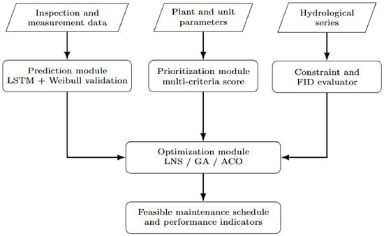
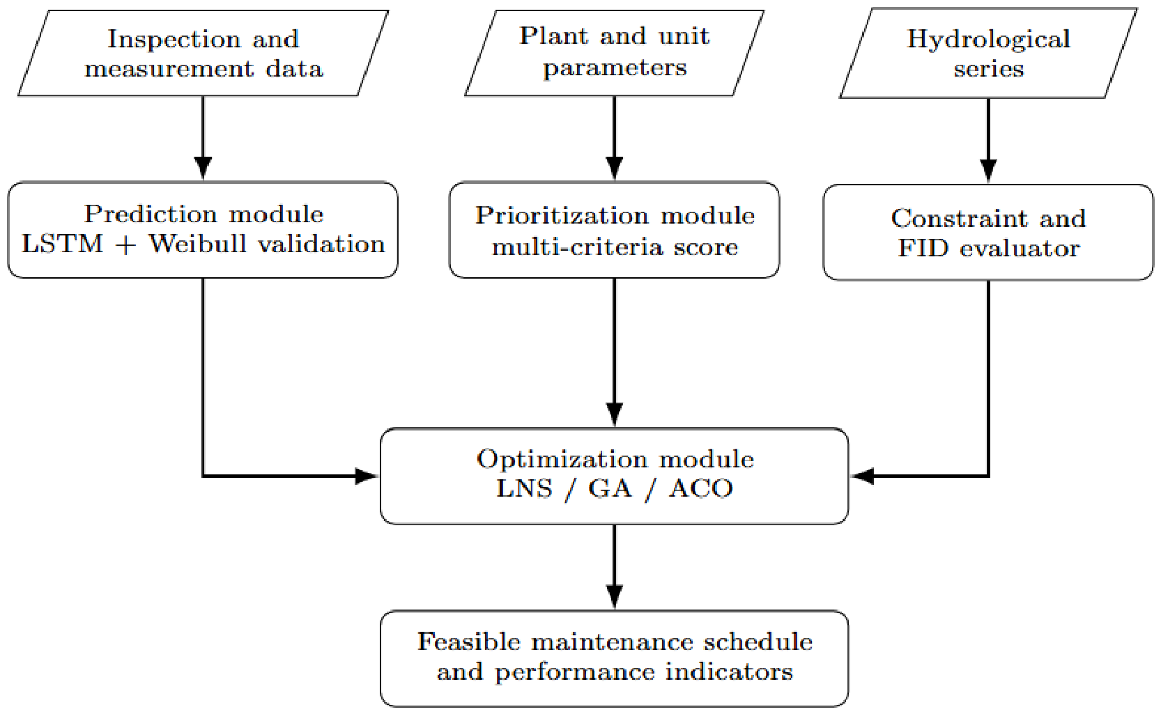
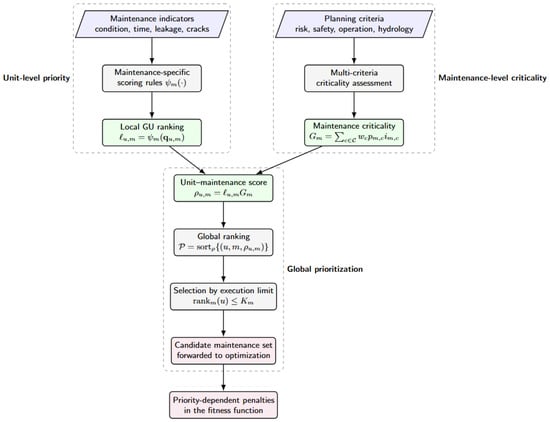
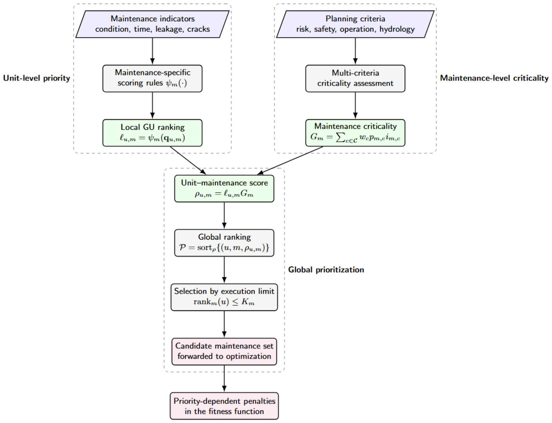
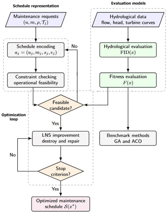
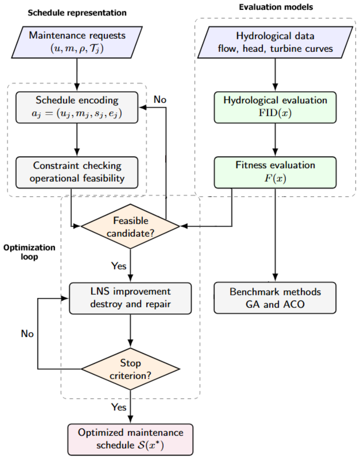
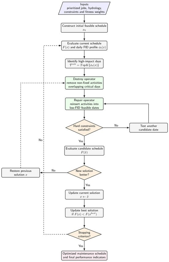
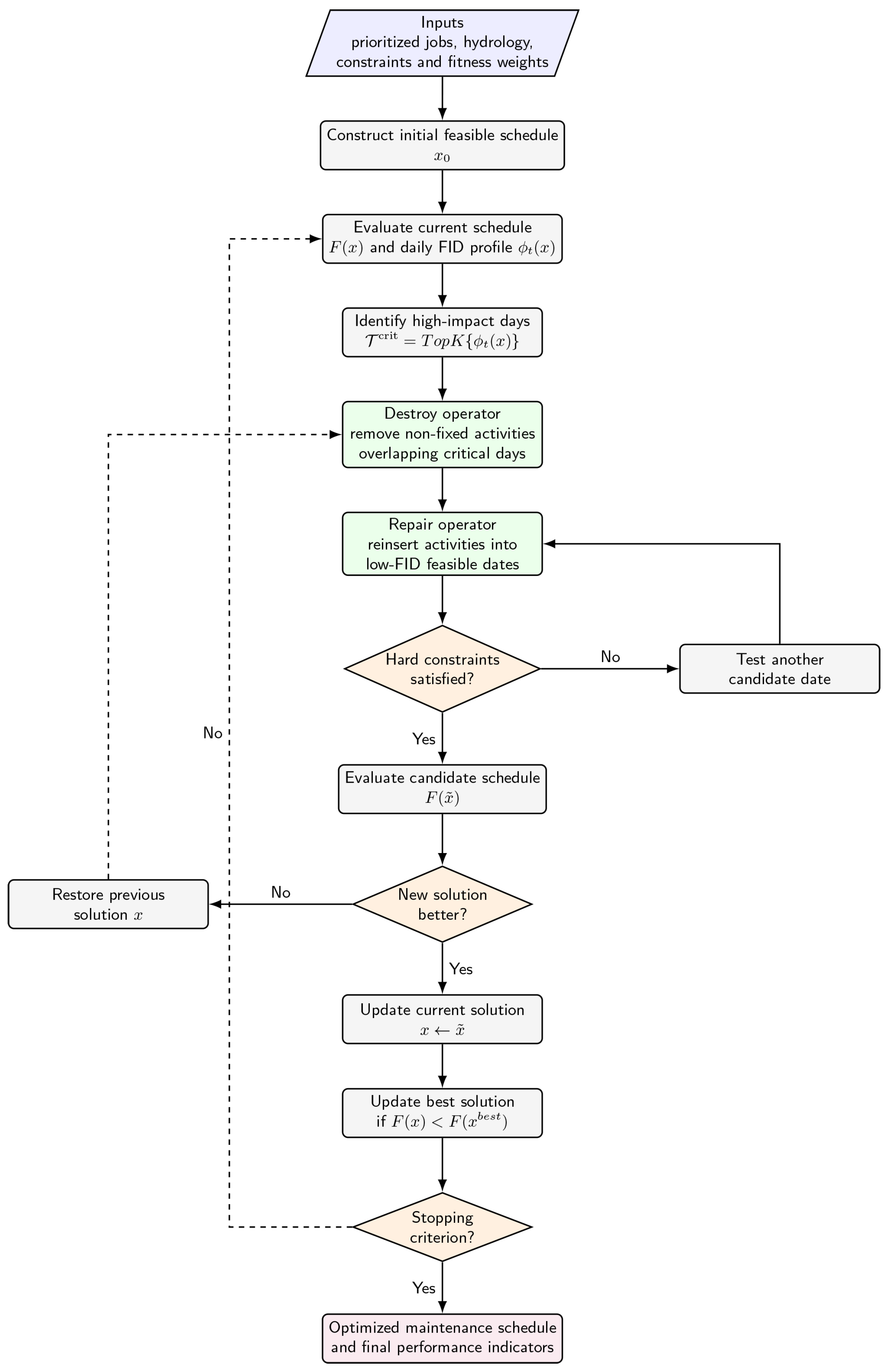
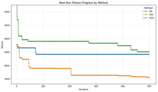
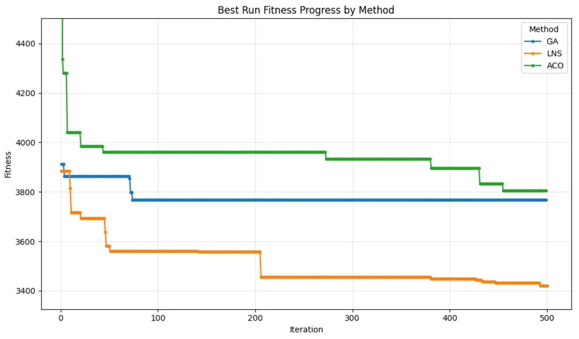
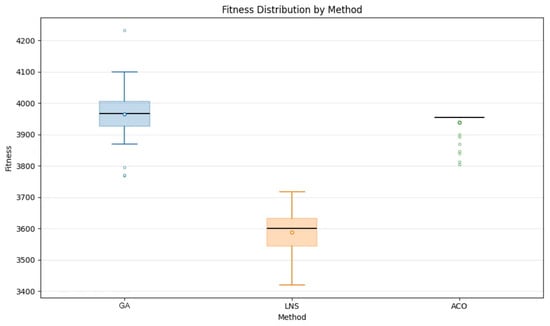
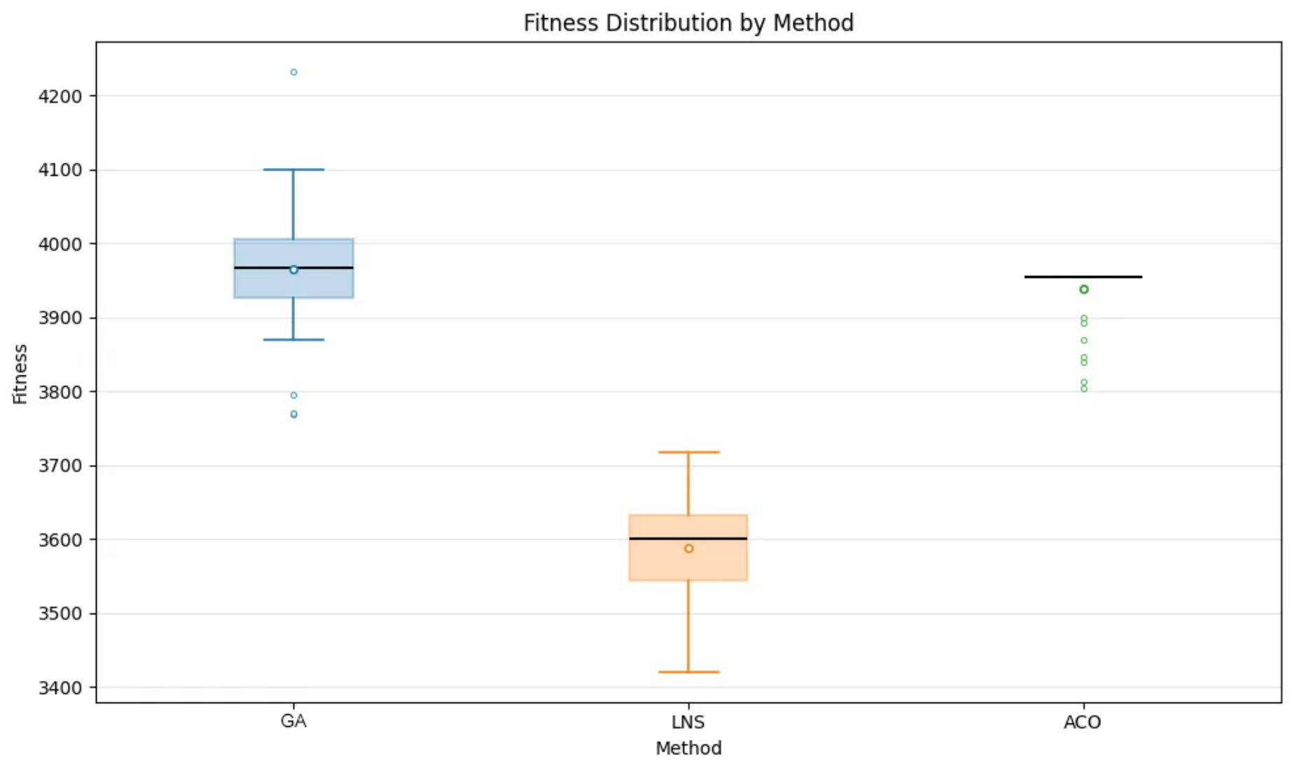
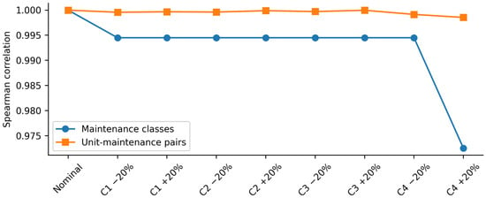
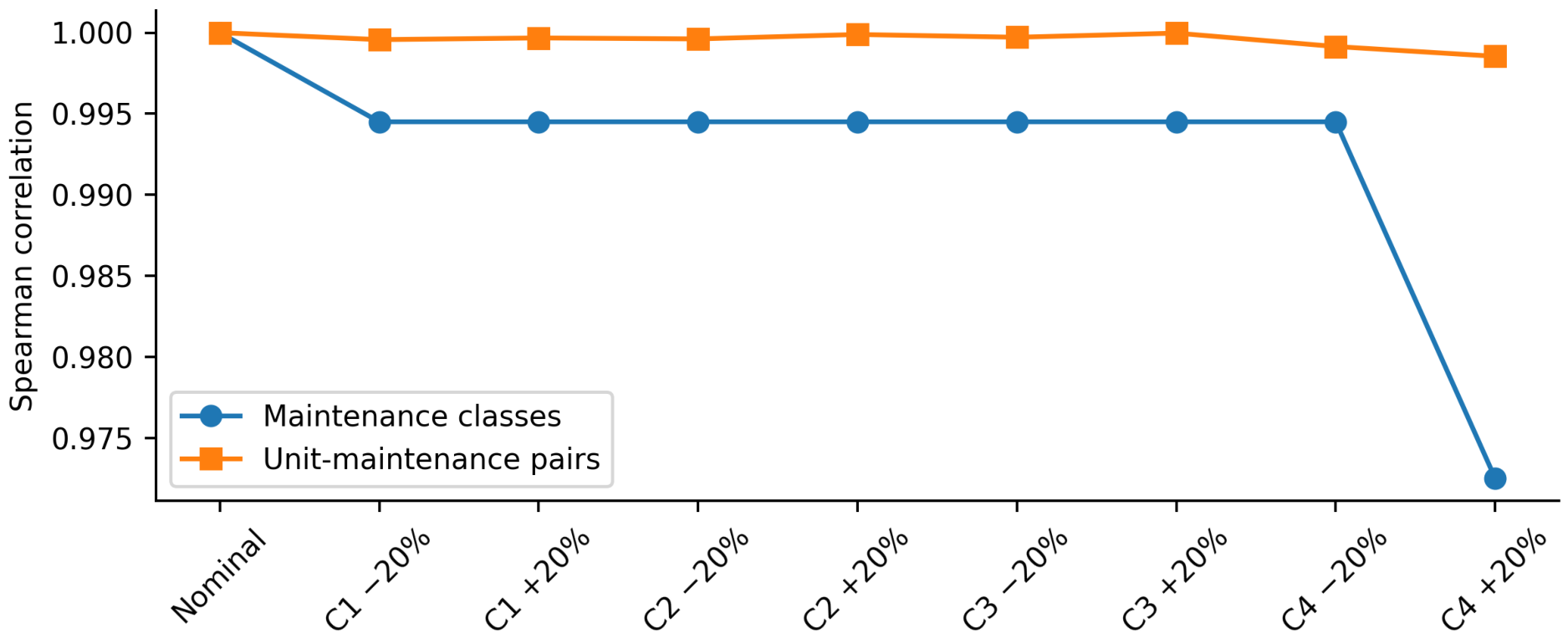
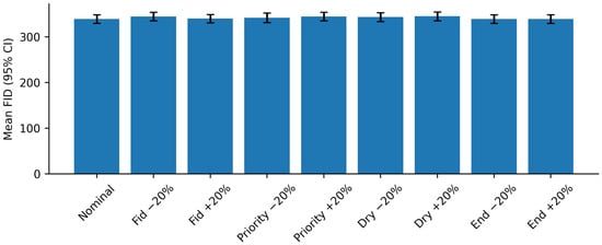
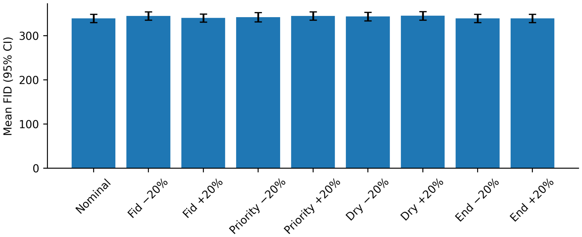
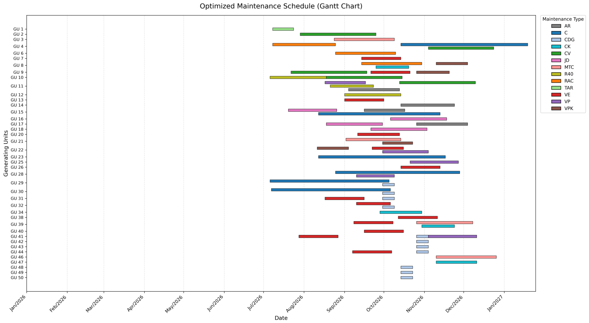
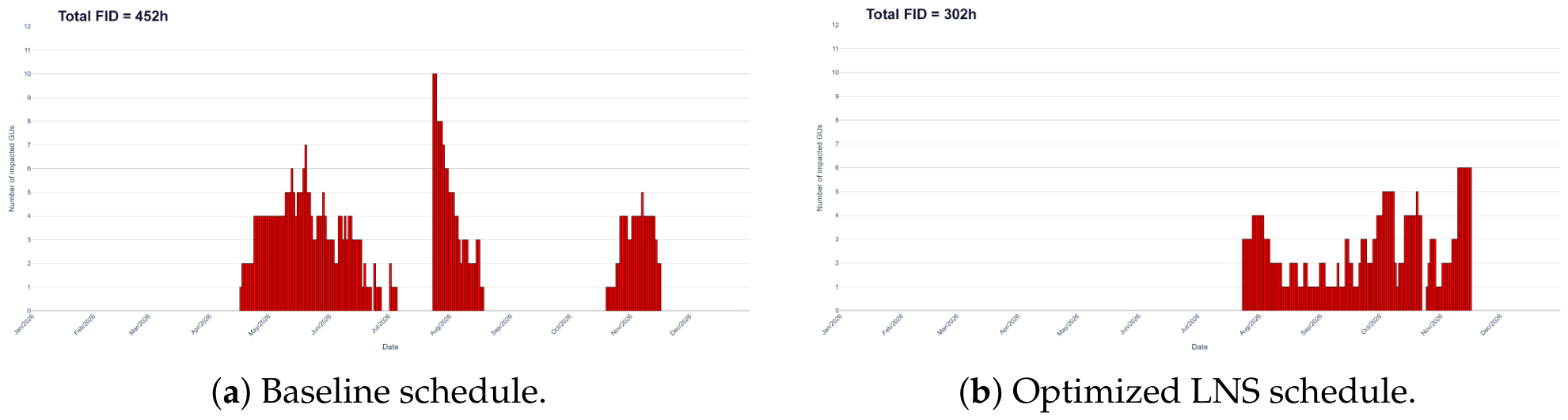

Disclaimer/Publisher’s Note: The statements, opinions and data contained in all publications are solely those of the individual author(s) and contributor(s) and not of MDPI and/or the editor(s). MDPI and/or the editor(s) disclaim responsibility for any injury to people or property resulting from any ideas, methods, instructions or products referred to in the content. |
© 2026 by the authors. Licensee MDPI, Basel, Switzerland. This article is an open access article distributed under the terms and conditions of the Creative Commons Attribution (CC BY) license.