


Abstract
Series resistance (Rs) is one of the most informative single parameters for the state of health of a photovoltaic (PV) string. Determining it without a curve tracer or interrupting production remains difficult, because maximum power point (MPP) tracking (MPPT) confines operation near the MPP. This study proposes a procedure in which the digital twin (DT) of an off-grid PV string with battery storage commands a scheduled, condition-gated current-voltage (I–V) sweep from the MPP toward open circuit through the current-limit register of the commercial charge controller. The reduced power continues to charge the battery. The single-diode model is fitted with the ideality factor and shunt resistance held fixed; the string-level Rs, inclusive of the DC cabling, is obtained by Levenberg–Marquardt iteration. In two measurement periods on the same four-module string, added series resistances of 0.33 to 1.18 Ω were recovered within 8% with a pooled regression slope of 0.97. Twelve clear-sky baseline sweeps over eight days agreed with a sample scatter of 3.4%. Feeding the in situ Rs back into the twin raised the operating power mean absolute percentage error (MAPE) from 7.1% to 12.9% when substituted alone and reduced it to 4.7% when the companion parameters were refit. A sweep takes about 144 s, costs about 5 Wh, roughly 0.1% of the daily yield. The results are limited to a single string at a single site and are presented as a feasibility study.
1. Introduction
The series resistance (Rs) of a photovoltaic (PV) array increases as the module degrades, for example through corrosion driven by the acetic acid released from the encapsulant [1]. It is a parameter that ohmically groups together the aging or failure conditions in array cells, cell metallization, metallization strip and strip-to-strip contacts, solder points, junction boxes and direct current (DC) cabling in a single quantity [2,3]. A 25-year field study of monocrystalline modules reported that while maximum power decreased by 23.3% and fill factor by 15.3%, open-circuit voltage decreased by only 2.28%. This decrease was mainly attributed to the increase in Rs resulting from metallic corrosion in the monitored series. The effect of the increase in Rs will be felt much more at the maximum power point (MPP) [3]. Increases in the Rs value are associated with degradation mechanisms such as contact corrosion and encapsulant discoloration [4,5]. The Rs value obtained in situ under real irradiance and temperature, showing a slow accumulation rather than a constant value obtained from laboratory measurements, has the ability to represent the monitored PV array [3,4,6].
Obtaining Rs from field data (current I, voltage V, temperature T, irradiance G) requires a PV model in which the parameters can be defined. For cost-effective calculation, the single-diode model (SDM), also known as the five-parameter model, which generates the current-voltage (I–V) characteristic with five parameters, is commonly used. In the SDM, the photocurrent (Iph), diode saturation current (I0), ideality factor (n), Rs, and shunt resistance (Rsh) are the five parameters [2,7]. Changes in each parameter involve physical changes; discoloration and similar optical losses lower Iph, while corroded contacts and interconnections increase Rs [3]. Therefore, the SDM needs to be fitted to physical changes at certain intervals, and these parameters need to be monitored over time; curve fitting in parameter values will become a condition monitoring process dependent on physical change [6]. The challenge is to obtain sufficient-quality I–V data from an array that continues to operate without interrupting power generation.
Extracting Rs directly on an active system presents significant practical challenges. The method of obtaining the I–V characteristic will determine the chosen analysis methodology. For example, in the International Electrotechnical Commission standard IEC 60891 [8], the internal Rs is determined by the specified temperature and irradiance correction procedures from the I–V curves obtained from the measurements. The estimators proposed by Sera et al. [9] use the slope of the I–V curve at points close to open circuit. Both have in common the need to scan the operating point over a wide range. This need requires an in-line I–V tracker or an equivalent physical actuator in a deployed array. Such studies without in-line additions rely only on passively recorded operating points and attempt to compensate for missing measurements during estimation. Comparing parameter extraction techniques on outdoor measurements with degradation emulated by external series resistors, Piliougine et al. [10] found that only a few methods reliably recover single-diode parameters after degradation has begun.
Operating points obtained under maximum power point tracking (MPPT) control are limited to the vicinity of the MPP. This narrow data window creates a mathematical problem during parameter estimation. While the Rsh parameter defined in the SDM is determined from the slope of the I–V curve near the short circuit, Rs is derived from the open-circuit region [11]. In a study simulating aging with series resistors, it was observed that the average of the Rs estimates made in the near-MPP region changed only slightly, but the standard deviation of the estimates increased by one order of magnitude [12]. This mathematical uncertainty is a condition that the present study also considers as an initial constraint.
Another study method predicted that the Rs estimates made in the area near the MPP would be biased. To overcome this problem, the standard deviation in the Rs value was reduced by averaging several hundred consecutive I–V curves obtained by fitting the SDM to narrow area values [12]. It was stated that this method is sufficient for stable value estimation. In the study [13], a polynomial function is obtained that describes how much this swelling increases, based on the observation that the determined resistance systematically swells as the fitting window narrows. At the time of the study, the Rs value corresponding to the narrow window is divided by the corresponding ratio in the polynomial to calculate the new Rs value. In the study conducted with automatic inverter voltage scans [14], the string inverter’s own I–V measurement capability is utilized, and a value read from the local slope near the MPP is expressed as the equivalent series resistance. However, it is not a physically meaningful SDM parameter. In another study with an inverter, the Rs parameter is obtained from the slope near the open-circuit voltage Voc with a micro-inverter on an 80 Wp module at only about 50 W/m2 [15]. However, the slope is insensitive to distributed series distortion and is limited by the low-irradiance window.
All studies cited so far have focused on achieving the target with a single estimate. A digital twin (DT), instead of a single prediction algorithm output with a computational value that occurs in this narrow field and contains multiple constraints, is treated as part of an ongoing model of the array. A DT is a virtual representation that works alongside a physical entity, exchanges data with it, and remains synchronized with its state throughout its operating life [16]. However, PV research has largely applied the DT approach in a one-way manner. In DTs used for multiple failure state analysis, the model predicts, the plant is measured, and the difference between the two values indicates failures [17]. Cloud platforms have extended similar approaches to large facilities [18]. Since SDM parameters correspond to physical degradation mechanisms, they fit well with these twins. It has been stated that SDM twins work even on low-cost embedded boards [19]. A systematic review [20] identifies bidirectional data flow and self-adaptation as two capabilities lacking in most PV DTs. That review refers to unidirectional twins as digital shadows. Field data do not flow back to update the model. The model only provides information to the operator.
The system analyzed here is an off-grid PV plant equipped with battery storage; this configuration is precisely what makes the control process in question cost-effective. In a grid-connected plant, any loss of power that could have been extracted from the MPP represents energy that cannot be fed into the grid. Consequently, a sweep process that shifts the operating point toward the open-circuit voltage results in a loss due to energy curtailment. In an off-grid plant, however, the charge controller already limits the charging current as the battery approaches full capacity. Therefore, current limiting is part of the system’s normal operation, and while the battery bank is in the bulk charging state, the power supplied from the PV array during the sweep continues to be stored. In this mode of operation, the energy deficit occurs only during the sweep process. On days when the battery reaches full charge, this deficit corresponds to an amount of energy that the controller would have restricted regardless. Section 5.4 quantifies this cost specifically for the plant under study.
The difficulties in determining the Rs value, a parameter that changes particularly with age, with unidirectional data flow without the application of targeted control techniques, are clearly evident. If a PV twin maintains the Rs value obtained from its initial calibration as the array ages, its predictions will slowly deviate from the actual array, and its own increasing error will become difficult to distinguish from the actual degradation. Without specialized hardware, it is necessary to periodically perform in situ Rs estimation on the array to maintain synchronization. This mode of operation has been shown to be difficult in the previous paragraphs. The architecture in this study allows the twin to obtain this estimation on a planned basis, provided the acquisition conditions in Section 3.3 are met. Monitoring and operation take place on a single interface. Therefore, data flow occurs in both directions. A planned measurement begins with writing to the current-limit register of the charge controller. For wide-range I–V data acquisition, the operating point moves toward open circuit, and the twin obtains the Rs estimate itself. In off-grid PV battery systems, the charge controller enables a physically meaningful in situ estimation of a parameter closely related to string aging. Whether this predictive model also needs updating is examined in Section 4.4, and live self-adaptation is left for future work.
This study demonstrates the feasibility of an in situ measurement approach for determining the Rs value of a PV string. The procedure was implemented at a single site on a string comprising four modules, spanning two measurement periods that included eight days of clear-sky conditions. Determining the remaining useful life of the modules or diagnosing fault conditions fell outside the scope of the study. While the digital twin architecture handles calibration, triggering logic, and model comparison, the estimate itself is obtained by actuating the charge controller. The study makes four contributions.
Firstly, the current-limit command of a commercial MPPT charge controller without an in-line tracker is used, through an actuation scheme, to record values over a wide range from the MPP toward the open-circuit voltage Voc while the battery continues to charge. Secondly, the wide range of data obtained from this actuation ensures that Rs is practically conditionally identifiable. Thirdly, it has been shown that the cost function has a sharp minimum under constant values of diode ideality factor and shunt resistance during SDM parameter estimation. The fact that multiple initialization tests, run from different starting points, converge to the same value each time confirms the consistency and stability of the estimated Rs value. Finally, known series resistances were physically added to the string in two measurement periods, and the identified Rs followed the applied increments across six levels. Pooling both periods, the regression of the recovered increment on the applied resistance gives a slope of 0.97, with a 95% confidence interval extending from 0.78 to 1.17. Offline testing was performed on the DT with the estimated Rs value. It has been shown that when this value is adjusted along with other parameters of the SDM, the accuracy of the operating point increases, while changing the value alone decreases the accuracy level. The rest of the article is structured as follows. Section 2 examines reference-based and hardware-free Rs inference and the related DT literature. Section 3 describes the actuation scheme, experimental platform, and estimation. Section 4 includes identifiability analysis, added-resistance validation, clear-sky reproducibility, and offline model comparisons. Section 5 discusses the uncertainty budget and scope, and Section 6 the results obtained.
2. Related Work
2.1. Reference-Based Series Resistance Extraction
The normative reference for determining series resistance is IEC 60891 [8,12,21]. According to procedure 4 of this standard, Rs must be derived from the full I–V curve. This section discusses studies on Rs obtained with a model fitted to the full characteristic curve from short circuit to open circuit. However, curve extraction in an operating array is rarely possible because normal operation takes place around the MPP, and the measured points will be in this narrow region. Kalliojärvi et al. gradually reduced the available measurement windows around the MPP and analyzed their estimates with the SDM [12]. It was stated that a slight increase in the average Rs was observed in the estimates, but the standard deviation increased from 0.0098 Ω in the full-curve case to 0.1055 Ω in the narrowest range. These data show that the estimation loses its repeatability. However, when the data range is kept wide, it shows that the simulated aging steps of 0.22 and 0.69 Ω are recovered. Lappalainen et al. argued that the narrow-window deviation problem can be compensated with a second-order polynomial model trained on ten full-interval reference curves and that if the amount of power that can be sacrificed does not exceed 2%, the mean deviation will also remain below 2% [13]. Piliougine et al. reported that a limited number of direct parameter extraction methods can reliably determine single-diode parameters in a module whose degradation was emulated with external series resistors [10]. All approaches in this group require a system-independent monitoring tool, even if only once, during the study or for calibration.
2.2. Hardware-Free In Situ Estimation
In studies within this group of methods, the system’s existing equipment was used for the I–V curve. These studies involved limitations such as measurement timing freedom and measurement range. Sera et al. estimated the series resistance from the dV/dI slope in a narrow window near open circuit, where the slope is governed mainly by that resistance, and translated the MPP power to standard test conditions (STC) [9]. Spataru et al. used the partial I–V scan feature implemented by existing commercial string inverters in their study [14]. They stated that five different parameters could be calculated with these scans. Firstly, the slope of the curve at 0.75 Impp (the MPP current) was accepted as the representative resistance value. The change in this value was classified as Rs increase, distortion, and shadowing with a high detection rate. However, these detections are not parameters of a circuit model; they are system status indicators. Pradeep Kumar et al. performed scans at dawn, the interval immediately before a grid-connected inverter starts supplying power [15]. By utilizing the wide range of changes in the string voltage while the inverter is idle, Rs was estimated with an offset correction from the open-circuit voltage slope and without requiring additional circuitry. Measurements at an irradiance level of 50 W/m2 are limited, and only a uniform increase in the slope near Voc is visible. Differences throughout the day are not discernible.
2.3. Digital Twins and Industrial Monitoring Platforms for Photovoltaic Systems
Supervisory control and data acquisition (SCADA), which plays a significant role in industrial systems, is also widely utilized in PV systems. Ferlito et al. described an Internet of Things (IoT)-based SCADA system for large-scale photovoltaic power plants. In this system, a hybrid storage solution featuring lightweight transport protocols and edge functionalities ensures the accessibility of historical records for performance analysis and predictive maintenance [22]. Meanwhile, Snytko et al. implemented energy flow indicators within an industrial SCADA system and, in a simulated benchmarking study, reduced the detection time for supply-demand mismatches from 15 min (associated with a conventional interface based on IEC 61724-1 parameters) to 3 min [23]. DTs have also been integrated into plant operation processes. Chen et al. synchronized a four-layer DT using module data from four large-scale power plants; they reported achieving an average fault diagnosis accuracy of 98.49% and a root mean square error (RMSE) of 0.0555 A in the reconstructed output characteristics [24].
DTs have generally been used as a residual generator in PV studies. Jain et al. ran a model of a panel-level energy conversion unit (the panel and its associated DC/DC converter) in real time with the actual hardware; they diagnosed faults using the residual vector, which is the difference between the outputs predicted by the model and the measured outputs [17]. Livera et al. brought it to the plant level on a cloud platform where contamination can be separated from long-term degradation [18]. As performed by Hueros-Barrios et al., an SDM twin can be implemented with an explicit Lambert-W solution on a low-cost embedded board [19]. In [25], a DT was integrated into the SCADA system of an actual renewable hydrogen microgrid at the system level, whereas in [26], a cognitive twin featuring a virtual reality interface was proposed for the interactive control of PV infrastructure. What is overlooked in these studies is self-adaptation. Online redefinition of model parameters for distributed twins in power systems has been demonstrated in a real-time collaborative simulation case study [16]. In [20], a systematic review of 61 DT studies in PV was carried out. The review indicated that only 3.3% of the studies met the criteria suggested by the authors, with bidirectional data flow and self-adaptation being missing features.
2.4. Positioning of the Present Work
As shown in Table 1, model-based Rs inference continues to be relevant. New studies continue to be published on module health assessment [27] and performance estimation without reference condition determination, i.e., without conversion to STC [28]. Tracer-based methods, when combined with external hardware, can perform curve extraction with high accuracy, but this comes at an additional cost. Hardware-free methods operate with their own equipment and compromise on scanning intervals or timing. DTs, which mostly operate with a one-way data flow from the facility to the model, observe the array and require external hardware for wide-range data acquisition. None of the approaches in the table combine on-demand wide-range data acquisition with a twin that processes data on site without requiring additional hardware. The closest example is the Voc slope method [9], which obtains the slope from curves recorded with a curve tracer rather than by actuating the plant’s own hardware. In this proposed study, the operation is performed over the current limit of the charge controller already controlled by the DT. It provides a wide-ranging sweep on demand without requiring a dedicated tracer. The resolution values in Table 1 are derived from the specific hardware used in each study rather than from a shared dataset. The Voc slope estimator from [9] was therefore applied to the same added-resistance sweeps used for the single-diode fit. Section 5.3 presents the increments recovered by each method and the offset between their absolute values.
Table 1.
Positioning of the present work against representative Rs-extraction and PV digital-twin approaches.
3. Materials and Methods
3.1. Procedure Overview
The proposed procedure repurposes the MPPT charge controller of the off-grid plant as a measurement actuator. Its current-limit register, provided by the manufacturer for battery protection, accepts a charging-current ceiling over the standard Modbus interface. Writing a value below the present operating current forces the controller to curtail charging, and the string operating point shifts from the MPP toward open circuit. The DT drives this response in a closed loop with the plant, as shown in Figure 1.
Figure 1.
Closed-loop in situ Rs measurement scheme. The DT sweeps the operating point from the MPP toward open circuit via the controller’s current-limit register and fits the SDM to the measured (V, I) points; the estimated Rs is evaluated offline. Red arrows denote the current-limit commands written by the DT to the controller, blue arrows the measured (V, I) data returned to the DT, and the numbered markers 1 to 5 correspond to the steps described in Section 3.1. Inset: measured points (hollow circles), MPP (filled circle), I–V characteristic (solid line) and the near-Voc slope used for Rs (dashed line).
In Step 1, the twin writes a predefined sequence of discrete current limits to the controller register. No hardware is added, disconnected, or bypassed. The command travels on the same serial link used for routine monitoring. In Step 2, the controller enforces each limit, and after a short settling time, the operating point stabilizes at a new position of the I–V curve, progressively closer to open circuit. The reduced output continues to charge the battery, provided the state of charge (SOC) permits energy absorption and the excess power remains unextracted rather than dissipated in a diversion load, so the sweep can run safely on an operational plant. In Step 3, the settled voltage, current, module temperature, and irradiance are recorded under stable environmental conditions, forming a set of operating points that extends from the MPP toward open circuit. In Step 4, the SDM is fitted to these points to estimate the series resistance, as detailed in Section 3.4. In Step 5, the accepted estimate is made available to the twin as an updated in situ value of one of its most aging-sensitive parameters. The register value is then restored, and the controller returns to normal MPPT operation. Automatic adoption into the live configuration is not enabled.
Step 5 is what separates this procedure from a one-off measurement. The estimate can be refreshed on demand whenever the triggering conditions of Section 3.3 are met. Section 4.4 examines how the refreshed value should be used without degrading the predictions of the model.
3.2. Experimental Platform
The procedure was implemented on a small off-grid system located in Antalya, Türkiye. The PV string, sensors, enclosure, and platform architecture are shown in Figure 2. The string consists of four series-connected 240 Wp half-cut monocrystalline modules (TT240-48PM12; TommaTech GmbH, Garching, Germany; 192 cells in series), oriented south at a 32° tilt. Each module is rated at STC with a maximum power of 240 W, an open-circuit voltage of 32.5 V, a short-circuit current of 9.11 A, and maximum-power-point values of 27.7 V and 8.67 A, with a short-circuit current temperature coefficient of 0.05%/°C; these label values are the inputs to the one-time calibration described below. Charging is handled by a commercial MPPT charge controller (SRNE MA2440N15; SRNE Solar Co., Ltd., Shenzhen, China), and the energy is stored in a nickel-manganese-cobalt (NMC) battery bank of 43 Ah nominal capacity, assembled from 43 Ah pouch cells (SK Innovation Co., Ltd., Seoul, Republic of Korea), supervised by a separate battery management system (BMS; Daly Smart BMS 8S–17S 80 A, Dongguan Daly Electronics Co., Ltd., Dongguan, China). A diversion load provides routine overcharge protection at full battery and remains inactive during measurements, since the trigger conditions of Section 3.3 require the bulk charging state. An adjacent meteorological station records plane-of-string irradiance with a Si reference cell (3S-IS; Seven Sensor Solutions, Istanbul, Türkiye), and module temperature is measured with a PT1000 element (3S-MT-PT1000, Seven Sensor Solutions) attached to the rear surface of one module at its geometric center. Every component is an off-the-shelf commercial device, and the only system-specific element is the software described below. The DC cabling between the string and the controller contributes to the total series resistance seen at the controller terminals. All values reported in this work therefore refer to this string-level quantity rather than to a single module, a definition made explicit in Section 3.4.
Figure 2.
Experimental platform: (a) four-module PV string and its sensors; (b) meteorological station; (c) enclosure (charge controller, BMS, battery bank); (d) architecture, with the power path (solid) and Modbus RTU over RS-485 (dashed).
All devices communicate with a single personal computer (PC) over the Modbus remote terminal unit (RTU) protocol, each on its own RS-485 link at 9600 baud with 8 data bits, no parity and one stop bit, which is the interface exposed by the charge controller, the BMS and the meteorological station; none of these devices offers Modbus TCP. The monitoring and control environment, developed in C# on the open-source .NET 8.0 platform (Microsoft Corporation, Redmond, WA, USA), polls each device once per second with a 3 s response timeout. Each reading is time-stamped by the PC clock, which is kept in local time (coordinated universal time, UTC+3). All instants reported in this paper, including the triggering window of Section 3.3, refer to this clock. The records are archived in daily comma-separated values (CSV) files, and the same environment hosts the DT and the estimation routine of Figure 1. Before deployment, the reference SDM parameters Iph, I0, Rs, Rsh and n are identified once at STC from the module datasheet values using a Levenberg–Marquardt algorithm and stored in the twin configuration (the One-Time Calibration block of Figure 1). The field procedure of Section 3.1 then re-estimates the series resistance against this baseline, with the ideality factor and the shunt resistance held fixed as described in Section 3.4. Table 2 summarizes the accuracy and resolution of this measurement chain, which enter the uncertainty considerations at the end of Section 3.4. The environment runs on a desktop PC with an Intel Core i7-7700 processor (Intel Corporation, Santa Clara, CA, USA), 16 GB of memory and Windows 11 (Microsoft Corporation, Redmond, WA, USA); the fit of Section 3.4 involves eight measured points, three parameters and at most 80 iterations from each of four initial vectors and places no particular demand on the computer.
Table 2.
Measurement chain of the experimental platform.
3.3. Sweep Protocol and Safety Limits
The sweep routine executes only when specific system prerequisites are satisfied. Before a trigger is accepted, the controller must operate in the bulk charging state with no active faults, and the battery SOC must exceed 40% so that the minor power deficit during measurement does not deplete an already-low pack. A minimum battery-side charging current of 8 A must be flowing, since below this level the sweep would cover a current range too narrow to be informative. Irradiance must be at least 700 W/m2, with a five-minute standard deviation below 3%. Local time must also fall between 11:00 and 15:00, a window that minimizes irradiance drift during the sweep. Execution is limited to once per day under automatic triggering, and the routine remains disabled unless explicitly authorized by the operator. The routine can be started in two ways. In automatic mode, which the operator enables and disables from the monitoring software, at most one sweep is started per local calendar day, at the first moment all of the above conditions hold, and a sweep that is aborted still uses that day’s slot. The operator can also start additional sweeps manually from the same software, with the same step sequence. In this study, the first sweep of each measurement day was started automatically, and the further sweeps of the same day, namely the repeated baselines and the added-resistance steps, were started manually.
Once triggered, the routine steps the controller current limit through seven predefined fractions of the charging current measured at the moment of triggering (0.97, 0.92, 0.85, 0.72, 0.55, 0.35, and 0.18), following an initial unconstrained baseline reading at the MPP. These fractions are deliberately unevenly spaced because output power is nearly insensitive to current variations near the MPP. An even spacing would collapse most of the steps into open-circuit conditions, leaving the region just below the MPP undersampled. This spacing approximately equalizes the voltage increments along the curve, since the exponential diode characteristic increases the voltage change per unit current toward open circuit. Each step is held for a 10 s settling period to eliminate transient effects before acquisition begins. Voltage, current, module temperature, and irradiance are then sampled for 8 s at 1 Hz, and the value retained for each step is the median of these eight samples; no other filtering is applied, and the register resolutions of Table 2 (0.1 V, 0.01 A) are the only quantization in the chain. A sweep is retained only if the initial baseline reading is stable. Sweeps in which the current spread during the baseline interval exceeds 0.5 A are discarded, since without a valid high-current baseline point the remaining points do not constrain the ohmic drop. The same 0.5 A limit is applied to each step, and a step whose samples spread by more than this value is dropped from the fit.
3.4. SDM Formulation and Parameter Estimation
The DT represents the string through an SDM formulated at the string level, with Ns = 192 cells in series and a single parallel branch (Np = 1), in line with SDM-based twin implementations reported for field monitoring [19]. The terminal current comprises three components
where Iph is the photocurrent generated by the illuminated junctions, Id is the current lost through the diode branch, and Ish is the leakage current through the shunt path. Both loss terms depend on the internal junction voltage V + I.Rs rather than on the terminal voltage alone. The diode current takes the exponential form,
and the shunt current takes the resistive form,
Rs therefore enters the model twice, inside the exponent of Equation (2) and in the numerator of Equation (3). Throughout this work, Rs represents a lumped string-level quantity that absorbs the cell interconnects, junction box and connector contacts, string cabling, and all other ohmic elements in the current path between the PV modules and the measurement terminals. Two thermal voltage scales are required. The per-cell thermal voltage, used in the saturation-current translation introduced below, is
where k is the Boltzmann constant, q the elementary charge, and Tc the measured cell temperature listed in Table 2. The combined string-level thermal voltage
incorporates the ideality factor n and the series cell count Ns into a single scale factor a, used in Equation (2) and in the Lambert-W solution.
The reference parameters of Section 3.2 are translated at runtime to the prevailing irradiance G and cell temperature Tc, following the De Soto formulation [2]. The photocurrent scales linearly with irradiance and includes the short-circuit current temperature coefficient αIsc; the saturation current follows the cubic-temperature bandgap law of [2] with Eg,ref = 1.121 eV and β = −2.677 × 10⁻⁴ K−1 for silicon. The shunt resistance scales inversely with irradiance and is clamped from below at 200 Ω to keep the branch physical under low-irradiance extrapolation. Two thermal voltage conventions coexist in this set. Equation (2) is written with the combined thermal voltage a of Equation (5), which contains Ns, whereas the saturation-current translation uses the per-cell Vt of Equation (4) and contains no Ns. No translation law is attached to Rs, which the model treats as condition-independent over the sweep envelope. It enters the formulation only as the quantity the procedure exists to estimate. The Nomenclature lists the symbols used in the estimation.
Equation (1) cannot be evaluated directly, since the current appears on both sides, once as the unknown and once inside the exponential through the I.Rs product. Rs is thus both the source of this implicitness and the parameter of interest. Jain and Kapoor [31] showed that the SDM admits an explicit solution through the principal branch W0 of the Lambert-W function, which gives the current as
where the corresponding argument is defined as
Evaluating Equation (6) yields the modeled current in closed form, without the per-point root-finding that would otherwise dominate the cost of an iterative fit. The same explicit formulation is available in the open-source pvlib library [32]. The deployed estimator does not call pvlib or any other external library; Equations (6) and (7), the Lambert-W evaluation, and the Levenberg–Marquardt update described below are implemented in native .NET code within the monitoring software.
The estimator fits Equation (6) to the (V, I) points collected by the sweep protocol of Section 3.3, with the free parameter vector p = [Iph, I0, Rs]. The optimization loop of Figure 1 performs three operations. The prediction step (a) evaluates Equation (6) at each measured voltage under the recorded G and Tc, giving the modeled currents Îi. The comparison step (b) forms the residual vector r of measured minus modeled currents over the N sweep points and accumulates their squares into the cost of Equation (8)
The adjustment step (c) updates the parameters with the Levenberg–Marquardt rule, used for PV parameter extraction in [33], in which the damping factor λ blends gradient descent with the Gauss-Newton step applied to the Jacobian J of r with respect to p.
The damping factor is initialized at 10−2 and multiplied by 0.3 after a successful iteration and by 10 after a rejected one. Each run terminates when the cost falls below 10−9, when λ exceeds 1012, or after 80 iterations, whichever occurs first. The fit is repeated from four initial parameter vectors that scatter Rs across 0.5 to 1.5 Ω within the search bounds of 0.02 to 5 Ω, so solutions outside the initialization range remain reachable, and the lowest-cost solution is retained. This keeps the deployed application free of additional dependencies. The settings above are identical for every run reported in this work, and no per-run tuning was applied. The parameters are constrained to physically admissible ranges, with Iph between 0 and 15 A, well above the string short-circuit current of 9.11 A at STC, I0 between 10−12 and 10−3 A, and Rs between 0.02 and 5 Ω. Because the cost function is unweighted, every retained point carries identical weight on the current scale, and the high-current baseline therefore exerts the highest leverage on the series resistance, where both the ohmic drop and the current sensitivity to it are largest. The identifiability of Rs is established by the curvature of the cost function around the retained solution rather than by convergence from arbitrary initializations, which is solver- and parametrization-dependent. That curvature is examined on measured sweeps in Section 4.
Two parameters remain fixed during the optimization. The ideality factor is kept at n = 1.0786, the value returned by the one-time calibration of Section 3.2 rather than taken from the literature. This calibration uses only the datasheet operating points and is independent of the field sweeps, so fixing n does not feed the sweep data back into the estimate; its effect on the absolute value and on the recovered increments is quantified in Section 5.1. It sits at the lower end of the 1.0 to 1.5 range reported for silicon modules by Villalva et al. [7], and fixing it follows the practice of recent Rs estimation studies [12,13]. Freeing n on a dataset of at most eight points between the MPP and open circuit would lead to compensation between n and Rs, since both shape the knee of the I–V curve. The shunt resistance is likewise excluded. Its signature appears near short circuit, where the shunt slope dominates the I–V characteristic, whereas the sweep of Section 3.3 moves in the opposite direction, from the MPP toward Voc. An optimization that frees Rsh would therefore extract information the excitation does not contain. For the same reason, the fixed value has little influence on the estimated Rs, as quantified in Section 5.1. The goodness-of-fit statistic R2 measures the agreement between the modeled curve and the measured points, but it cannot confirm parameter uniqueness. Parameter sets with distinct Rs values can reproduce a narrow section of the characteristic almost equally well, so a high R2 does not validate the recovered Rs. Confidence in the estimate rests instead on the high-current baseline point of Section 3.3, which carries the greatest leverage on the ohmic drop where it is largest, and on the independent added-resistance validation of Section 4.2. In this procedure, R2 serves only to reject corrupted sweeps before they reach the estimator.
Four uncertainty sources dominate the estimation. The measurement chain introduces the calibration residuals quantified in Section 3.2. The cell temperature enters Equations (4) and (5) and the temperature-translation laws uncorrected for sensor placement. Environmental conditions can drift over the 144 s sweep window even under the stability gate of Section 3.3. The fixed ideality factor transfers part of any error in n into Rs through the compensation described above. These uncertainties are common to all field-monitoring applications, and this work does not claim to eliminate them. The estimate is expressed in ohms and validated against added resistance in Section 4.2, though its absolute agreement with the physical series resistance remains conditional on the fixed n and Rsh. Successive estimates obtained under the same fixed n and an identical protocol are therefore evaluated against a commissioning baseline, and the reproducibility reported in Section 4.3 is the figure of merit for change tracking.
4. Validation and Results
The validation framework evaluates the conditioning of the estimation problem, the accuracy of the estimated resistance, its day-to-day reproducibility, and the behavior of the twin when the in situ value is fed back into the deployed model. Within the scope of this feasibility study, Rs is evaluated as a total string-level quantity rather than decomposed into individual module contributions, since the lumped resistance represents the ohmic losses at the controller terminals and includes the DC cabling and connector contacts in the current path. Direct comparison with factory datasheet values is omitted, since the deployed string operates under field conditions.
4.1. Conditional Identifiability of the Estimated Resistance
The conditioning of the fit was examined in two complementary ways on the wide MPP-toward-Voc sweep of 28 June at 14:32 shown in Figure 3 and Table 3. The first fixes Rs across a grid of trial values and re-optimizes Iph and I0 at each point, so that the location of the minimum does not depend on the initialization. The resulting cost profile exhibits a single sharp minimum rather than an extended flat valley, with the cost rising steeply on both sides of the optimum. Rs is therefore tightly localized by the data, with no broad region of near-equivalent solutions, as illustrated in Figure 4. That curvature is quantified against a principled far point in Section 5.2.
Figure 3.
Actuated sweep on 28 June at 14:32 with the SDM fit; parameters are listed in Table 3.
Table 3.
SDM fit parameters.
Figure 4.
Identifiability analysis of the estimated series resistance for the 28 June sweep at 14:32, showing (a) the cost profile under a fixed Rs grid and (b) multi-start estimates as a consistency check.
The second check evaluated the full three-parameter fit, optimizing Iph, I0, and Rs from ten independent initializations spanning the search range. This check was carried out with an independent C# implementation of the same model (.NET 8.0), with I0 fitted in log10 space to remove the scale ill-conditioning that otherwise stalls the solver at the parameter bounds, and the lowest-cost solution was retained. The identifiability argument rests on the profile curvature above rather than on a convergence count, and the multi-start result serves only to confirm consistency. The cost profile minimum lies at 1.489 Ω, while the multi-start best-cost solution and the deployed Levenberg–Marquardt fit of Figure 3 both give 1.488 Ω. The three agree to within 0.1%, well within the day-to-day spread of Section 4.3. Both checks remain conditional on the fixed values n = 1.0786 and Rsh = 8635 Ω.
At the final solution, the Jacobian matrix remains numerically stable, which reflects the localized sensitivity of the high-current data points to the series resistance within the internal junction voltage calculation.
4.2. Added-Resistance Validation: Gain, Reversibility, and Solver Cross-Check
External resistors of known value were connected in series with the string as an independent reference. No module was dismounted (Figure 5). The bank consists of unbranded aluminum-housed 50 W chassis-mount power resistors of 0.10 Ω nominal value (±5%, ±350 ppm/°C). Two measurement periods were run on the same string. Two levels were added on 28 June, and four levels, a return step and a removal step, on 8 September. Each June step was measured beforehand by the voltmeter-ammeter method, with the voltage read directly at the step terminals, giving 0.33 and 1.05 Ω. In September, the same quantity was measured at the operating current with the bank inserted, the terminal voltage read with a handheld multimeter (UT195DS; Uni-Trend Technology (China) Co., Ltd., Dongguan, China) and the string current taken from the controller register (Table 2). Three units gave 0.359 Ω and ten units 1.179 Ω, or 0.117 Ω per unit with no measurable offset. The five-unit and seven-unit steps were not measured directly. They were assigned 0.593 and 0.827 Ω from this per-unit value. All added-resistance sweeps ran under operator authorization. Routine operation executes a single automatic sweep per day.
Figure 5.
Series-resistor bank used for the added-resistance experiment.
The June sweeps were taken in immediate succession within a 0.5 °C module-temperature window and under closely matched irradiance (Table 4). Only the added resistance changed between them. With nothing added, the estimate was 1.488 Ω. Adding 0.33 Ω raised it to 1.801 Ω and adding 1.05 Ω raised it to 2.604 Ω, for recovered increments of 0.313 and 1.116 Ω, or −5% and +6% of the applied values. The September sequence began with three baseline sweeps between 11:07 and 11:46, which gave 1.408, 1.401 and 1.421 Ω and a mean of 1.410 Ω. The four levels were applied between 12:34 and 13:52, at module temperatures of 51 to 53 °C and irradiance of 1060 to 1091 W/m2. The estimates were 1.796, 2.041, 2.282 and 2.514 Ω. Recovered increments of 0.386, 0.631, 0.872 and 1.104 Ω fall within +8%, +6%, +5% and −6% of the applied values. Returning the bank to 0.593 Ω gave 2.076 Ω, 0.035 Ω above the first reading at that level. The bank was removed at 14:08. A sweep at 14:35 gave 1.514 Ω, 0.104 Ω above the morning baseline, and the first sweep of the following day returned 1.387 Ω, within 2% of it. The offset seen immediately after removal did not persist and is attributed to the re-termination of the string cable during the removal.
Table 4.
Controlled series-resistance steps (added resistance), 28 June and 8 September 2026.
Regressing the recovered increment on the applied resistance over all six levels gives a slope of 0.97, with a 95% confidence interval (CI) of 0.78 to 1.17 and a coefficient of determination of 0.9789 (Figure 6). Only the six applied levels enter the fit. The origin is excluded because each increment is referenced to the baseline sweep of the same day, and with nothing added, that difference is zero by construction rather than by measurement. Including such a point would raise the coefficient of determination without adding information. A regression on the four measured levels alone, without the two assigned ones, gives a slope of 0.973 and a wider interval. The six-level result therefore does not depend on the assigned values. The June (V, I) sets were also refitted with an independent implementation of the SDM, using a different optimizer and root-finding scheme, to rule out an artifact of the deployed solver. The two agree to within 0.001 Ω on all three sweeps (Table 5).
Figure 6.
Recovered increment of the series resistance versus the applied resistance for the six levels of the two measurement periods, each referenced to its same-day baseline, with the pooled linear fit and the 1:1 line.
Table 5.
Solver cross-check on the added-resistance sweeps.
4.3. Reproducibility Across Clear-Sky Days
Reproducibility was evaluated on clear-sky baseline sweeps taken on 22, 25, 26, 28, 29 and 30 June and on 8 and 9 September. Twelve of the fourteen sweeps acquired on these days met the acquisition criteria and yielded estimated series resistances between 1.343 and 1.488 Ω with a mean of 1.411 Ω (Figure 7) and a coefficient of variation of 3.4%. Two sweeps, on 22 June at 13:14 and 28 June at 11:02, were discarded for the absence of a valid high-current baseline point, the current spread during the baseline interval having exceeded the stability limit of Section 3.3, a criterion defined before the measurement periods. The June mean of 1.404 Ω and the September mean of 1.417 Ω differ by 0.013 Ω, about a quarter of the sample standard deviation, so the two measurement periods are consistent with an unchanged string.
Figure 7.
Clear-sky reproducibility of the baseline Rs estimate over the twelve retained sweeps of June and September, with the mean and the ±1σ band. The labels (1) to (3) denote the order of the repeated sweeps taken on the same day.
The twelve sweeps span a module temperature range of about 18 °C (Table 6), from 32 to 50 °C, and no temperature trend is resolved in the recovered Rs at this level of scatter. The expected change over this span is comparable to the observed spread, so the present dataset cannot separate the two. These results establish the preliminary feasibility of reproducibility tracking under operational conditions, and the deployed system continues to accumulate clear-sky sweeps, which will allow tighter tolerances to be defined over time.
Table 6.
Baseline sweep values and measurement conditions.
The 3.4% coefficient of variation also sets the detection latency of the indicator. Aging-related changes in Rs accumulate slowly, so a single sweep cannot resolve them against this floor. Averaging lowers the floor in proportion to the square root of the number of sweeps, so a monthly aggregate of the order of eight sweeps meeting the acquisition criteria of Section 3.3 would reduce the effective scatter to roughly 1.2%. Establishing this rate requires a longer observation period than the present dataset covers.
4.4. Offline Model Comparison of Parameter Transfer
The final check examines how the in situ estimate behaves inside the operational software. The twin runs on a configured parameter set in which Rs = 0.843 Ω (Model M1), formed from the datasheet-derived contribution of the four series modules, 0.343 Ω, and the DC cabling and terminal resistance of 0.5 Ω, measured directly on the disconnected cable by the voltmeter-ammeter method. The two terms differ in origin, since the cabling term is a direct measurement while the module term is inferred from the datasheet operating points. The in situ estimate of 1.488 Ω exceeds the configured total by 0.645 Ω and replaces that inferred term with a value obtained on the string itself. Table 7 compares five parameter sets. The sets of Models M3 and M5 were refit on the 28 June record, and all five were evaluated on 29 June, so no parameter was fitted on the evaluation day. The operating error is computed over the 1 Hz record of that day, comprising 64,189 samples in the bulk charging state.
Table 7.
Offline model comparison of parameter transfer between the sweep and operating regimes.
Substituting the measured Rs alone (Model M2) raises the operating mean absolute percentage error (MAPE) of the predicted string power from 7.1% to 12.9%. The configured Iph and I0 were identified in the one-time datasheet calibration of Section 3.2, and after the substitution, they no longer match the resistance they are paired with. Model M3 takes Rs and I0 from the sweep fit. Only Iph is refit on the operating record. The sweep gives an I0 three times the configured value, and with that value held fixed, the refit reaches the operating power by pushing Iph up to 12.7 A at STC. This is 40% above the datasheet short-circuit current of 9.11 A. In the single-diode model, the two currents differ at STC by no more than the leakage through Rsh, which is a few milliamperes here, and the value is therefore not physically admissible. The configured set M1 carries Iph = 9.11 A. The refit of Model M5 described below returns 8.91 A. The operating error of M3 reaches 15.2%. Model M4 transfers the complete sweep-fitted set. The operating error rises to 36.4%, even though that same set reproduces the actuated sweep at an RMSE of 0.042 A. The sweep lasts 144 s under nearly constant conditions, whereas the operating record covers a full day of varying irradiance and temperature. Model M5 holds Rs at the measured value and refits Iph and I0 on operating data, and the operating MAPE returns to 4.7%, below the configured baseline on 29 June and on the two further evaluation days examined, by margins of 1.7 to 2.4 percentage points. Fixed-parameter sets vary by more than two percentage points between days, so the improvement is reported as a range rather than a single figure. Before the monitoring software replaces the configured set with an in situ estimate, the sweep must have passed the acquisition gate of Section 3.3, the change from the commissioning baseline must exceed the single-sweep detection limit of about 0.14 Ω (3σ of the clear-sky scatter of Section 4.3, Table 1), and Iph and I0 must be refit together with Rs, with the refit Iph not exceeding the datasheet short-circuit current of 9.11 A. The refit set should lower the operating MAPE on independent days, as in Table 7, before it is adopted. Automatic adoption remains disabled in the present implementation.
The contribution of the twin in this work is the measurement-side link, namely the ability to command the sweep and recover a physical parameter over the existing interface. The transfer results show how that parameter enters the predictive model, since the measured Rs is compatible with operating-point accuracy but only when the companion parameters are refit alongside it. The sweep constrains the parameter set tightly while the operating point does not, which is the reason the actuated sweep is needed.
5. Discussion
Changes in Rs are resolved reliably, since the added-resistance tests recover known increments over six applied levels with a regression slope of 0.97 and a 95% confidence interval of 0.78 to 1.17. Absolute values carry a wider uncertainty, since the fixed ideality factor maps onto an asymmetric tolerance band of approximately +5% to −17% on the extracted resistance (Section 5.1). The two claims are separable because an added series resistance enters the model exactly as Rs does, so a misspecified ideality factor displaces the extracted value by an offset that is common to both sweeps and cancels in the increment. Identifiability rests on the curvature of the cost function around the retained solution, conditional on the fixed ideality factor and shunt resistance, as established in Section 4.1.
5.1. Absolute Uncertainty in the Extracted Resistance
The parameter extraction fixes the ideality factor at n = 1.0786 and the shunt resistance at Rsh = 8635 Ω, treating Iph, I0 and Rs as free variables. Under these conditions, Rsh has negligible influence on the sampled points. Refitting the 8 September baseline sweep of 11:46 with Rsh fixed at 86, 864, 8635 and 86,353 Ω gives Rs = 1.398, 1.420, 1.422 and 1.422 Ω, a total shift of 1.7% over three orders of magnitude, below the 3.4% reproducibility scatter. The reason is that the sweep covers the region between the MPP and open circuit, where the shunt current at the calibrated value is about 14 mA at 120 V, below 1.3% of the smallest string current retained in the sweep and below 0.2% of the baseline current, so the shunt branch does not shape the part of the characteristic from which Rs is determined; the same property that prevents the sweep from identifying Rsh prevents an error in Rsh from propagating into Rs. The ideality factor is therefore the controlling assumption for absolute uncertainty. Evaluating n across the plausible crystalline silicon range while refitting Rs at each step shifts the extracted resistance asymmetrically, from approximately +5% at n = 1.0 to −17% at n = 1.35, reaching −25% at n = 1.5. A lower assumed ideality factor inflates Rs modestly, whereas a higher value deflates it more steeply. Over the plausible interval n ∈ [1.0, 1.35], the uncertainty band is +5% to −17%, corresponding to +0.08 and −0.25 Ω at Rs ≈ 1.49 Ω.
This one-at-a-time analysis serves as a first-order uncertainty budget. Even at the lower bound of the band, 1.24 Ω at n = 1.35, the estimate remains well above the configured value of 0.843 Ω. The added-resistance tracking of Section 4.2 is unaffected by the assumed n, since an added series resistance enters the model exactly as Rs does and a misspecified ideality factor displaces both sweeps by a common offset that cancels in the increment. Table 8 puts this to the test. Refitting every baseline and loaded sweep of both measurement periods at n = 1.00, 1.20 and 1.35, with Ns and Rsh held at their deployed values, moves the mean baseline value from 1.41 Ω to 1.49, 1.30 and 1.17 Ω, whereas the six recovered increments change by at most 0.035 Ω, 4% of the applied value, and the pooled slope stays between 0.97 and 1.00, inside the confidence interval of the deployed fit in every case. The day-to-day coefficient of variation (CV) of the twelve baselines rises from 2.9% at n = 1.00 to 5.8% at n = 1.35. The quantity recovered by the fit is the SDM-effective series resistance at the controller terminals, and its absolute interpretation is bounded by that definition.
Table 8.
Absolute estimate and recovered increments at four values of the ideality factor.
The fixed value n = 1.0786 comes from the same one-time calibration that produced the configured Rs, but the calibration constrains the two parameters to different degrees. The ideality factor is a diode property of the cell, confined to a narrow range for crystalline silicon, and the sensitivity analysis above spans that entire range, so its possible error is bounded in advance and contained within the reported band. No comparable bound applies to the series resistance, which is why it is the parameter measured on the string rather than assumed. Holding n fixed also keeps successive estimates comparable, since a value refitted at each sweep would let parameter compensation contaminate the difference between them.
The estimate leans on the high-current baseline point, where the sensitivity is governed by the current rather than the voltage. Refitting the 28 June sweep with the baseline current displaced by ±0.05 A moves the recovered resistance by ±0.023 Ω, about 1.5%, with a linear response of roughly 0.47 Ω/A, whereas a 0.1 V displacement of the baseline voltage moves it by 0.003 Ω. Propagating the register resolutions of Table 2 through these sensitivities shifts the estimate by about 0.3%, well below the 3.4% day-to-day spread of Section 4.3. That spread is not set by the resolution of the measurement chain, and over the eight days involved it cannot reflect physical change in the string.
That figure comes from displacing a single point by one register step. To propagate the register noise formally, the Monte Carlo method of the Joint Committee for Guides in Metrology (JCGM) document JCGM 101 [34] was applied, as used for PV cell models by Tolić et al. [35] and for noise-corrupted I–V curves by Mesbahi et al. [36]. In each trial k, the eight retained points of a sweep are perturbed independently according to Equations (9) and (10),
where R(−δ, +δ) is the rectangular distribution, the assignment JCGM 101 prescribes when only the bounds of an error are known [34]. Two bound sets were propagated, half the register resolution of Table 2 (δV = 0.05 V, δI = 0.005 A) and the full register accuracy (δV = 0.1 V, δI = 0.01 A). The perturbed points are refitted with the estimator of Section 3.4 and the series-resistance component of the solution is retained,
and the standard uncertainty follows from the M trial values,
with the 95% coverage interval of Equations (11) and (12) taken between the 2.5th and 97.5th percentiles of the M values. Each of the twelve clear-sky baseline sweeps of Section 4.3 was propagated with M = 1000 trials. At half resolution, the standard uncertainty is 0.008 Ω (0.6%). At the full register accuracy, it is 0.017 Ω (1.2%), and the 95% coverage half-width is 0.033 Ω. Across the twelve sweeps, the value ranges from 0.015 to 0.023 Ω, with no dependence on the irradiance or temperature of the sweep. In no sweep does the mean of the trials differ from the unperturbed estimate by more than 0.001 Ω, which rules out a bias from the noise. Since variances add, the full-accuracy figure explains about one eighth of the variance of the 0.048 Ω day-to-day scatter of Section 4.3. The remaining 0.045 Ω is not of instrumental origin. The estimate is also sensitive to the module temperature entering Equations (4) and (5); refitting the 28 June sweep with the temperature raised by 13 °C lowers Rs by 0.044 Ω, about 0.003 Ω/°C, so an error of 20 °C in the rear-surface reading would shift the absolute value by 0.07 Ω (4.5%) without affecting the recovered increments. The reading comes from a single rear-surface sensor, so it carries a steady offset from the junction temperature and lags it during the 144 s sweep. Both effects enter through the same sensitivity of about 0.003 Ω/°C; the drift observed in the rear-surface record during a sweep stays below 1 °C in most sweeps and is below the standard uncertainty of a single estimate, while the steady offset is common to the baseline and loaded sweeps of a day and largely cancels in the recovered increments.
5.2. Goodness of Fit Versus Parameter Identifiability
A high R2 shows that the model reproduces the measured curve. It does not show that the parameters behind that curve are correct, because the free parameters can absorb an error in one of them. The 28 June sweep demonstrates this directly. When Rs is held at the configured 0.843 Ω and the remaining parameters are refitted, the model still matches the measured points with R2 ≈ 0.984, although 0.843 Ω is smaller than the fitted value of 1.488 Ω by a factor of 1.8. Fit quality alone therefore cannot distinguish a correct series resistance from one that is different by nearly a factor of two, and near-MPP extraction methods face the same limitation in the field [10].
The evidence used here is different. Rather than asking how well the model fits at the optimum, it asks how quickly the fit deteriorates when Rs is moved away from it. Figure 4 shows this by fixing Rs at a series of trial values and refitting the remaining parameters at each one. The fit error rises steeply on both sides of the minimum, reaching approximately 370 times its minimum value at 4.8 Ω. A weakly determined parameter would instead give a shallow valley, in which distant values fit almost as well as the optimum. This steep rise is a direct consequence of the wide actuated span, and it is obtained without the full-curve reference data that near-MPP corrections require, whether the correction trains a polynomial on tracer-acquired curves [13] or averages across a large number of curves [12].
5.3. Positioning Against Existing Approaches
Series resistance can be measured in the field either with a curve tracer, which supplies the full characteristic at the cost of dedicated hardware and an interruption, or without one, in which case the method works with whatever excitation the plant already provides. Each hardware-free method concedes a different property. The open-circuit slope was demonstrated on curves from a dedicated tracer [9], the pre-startup capture is confined to a short window at dawn [15], and the inverter-based indicators are empirical signatures rather than circuit parameters [14]. The present procedure concedes none of these three at once, since it adds no instrument, runs on demand within the daytime window of Section 3.3, and extends from the MPP toward open circuit.
Of the three, only the slope estimator of [9] can be applied to the sweeps recorded here. The methods of [14,15] obtain their I–V points from a grid-connected inverter, and this off-grid system has none. The estimator takes dV/dI from the two lowest-current points of each sweep, closest to open circuit. It subtracts the diode correction term at the operating conditions and refers the result to STC. It was applied to the September sweeps with added resistance, so both methods work on the same data. On the three baseline sweeps, it gave a mean of 2.023 Ω, against 1.410 Ω from the SDM fit. With the bank inserted, it returned 2.399, 2.663, 2.826 and 3.166 Ω. Subtracting the baseline leaves increments of 0.376, 0.640, 0.803 and 1.143 Ω. Table 9 lists them next to the SDM increments of 0.386, 0.631, 0.872 and 1.104 Ω and the applied 0.359, 0.593, 0.827 and 1.179 Ω. The offset of about 0.61 Ω is mostly the diode term at STC, not series resistance. It appears in the baseline and in every loaded sweep alike. It therefore cancels in the increment. On the increments, the slope estimator reaches a mean absolute error of 0.031 Ω, against 0.046 Ω for the SDM fit. The difference of 0.015 Ω lies below the standard uncertainty of a single estimate, 0.017 Ω (Section 5.1). Four levels cannot decide between the methods. They differ in the absolute value. That is the quantity the twin uses in Section 4.4, and the SDM value is the one passed to it.
Table 9.
Same-data comparison of the two estimators on the September sweeps with added series resistance.
The cost of that combination is accuracy. The absolute value carries the +5% to −17% band of Section 5.1, and the smallest increment demonstrated here is 0.33 Ω. A change of 0.1 Ω is about twice the day-to-day scatter of Section 4.3 (0.048 Ω) and is therefore not resolvable from a single sweep.
What makes the combination possible is the twin rather than the sweep alone. The fixed parameters come from the commissioning calibration it already holds, the trigger conditions are evaluated against its model of the operating state, and the parameter transfer of Section 4.4 is a question that arises only where a deployed model exists. The measurement loop is closed in both directions, which addresses the missing bidirectional flow identified in the review of Section 2.3 [20]. Automatic adoption into the live configuration remains disabled for the reason given in Section 4.4.
5.4. Disruption Cost
Curtailing the operating point introduces a local power deficit that can be quantified. Integrating the difference between the maximum-power baseline and the delivered power over the dwell intervals gives a total energy loss of approximately 4.7 to 5.0 Wh per sweep, depending on how far toward open circuit the sweep extends, with a representative full-span sweep accounting for roughly 5 Wh. Under clear-sky conditions at this site, a single daily sweep corresponds to about 0.1% of the daily energy yield. The power generated during the sweep continues to charge the battery, so the harvested energy is not dissipated and the only loss is the deficit itself. In an off-grid system, this deficit carries no export value, and on days when the battery reaches full charge, the controller would curtail an equivalent amount regardless, which places the practical penalty below the calculated figure. This bounded cost is what buys the wide identifiable span that near-MPP methods cannot provide and that conventional tracers obtain only by disconnecting the string.
5.5. Scope and Limitations
Series resistance increases over a module’s service life [1,3], which makes tracer-free measurement useful as an input to condition-monitoring pipelines. The present study covers a single string at a single site, without the extended time series needed to separate long-term resistance trends from short-term scatter, and the reproducibility dataset comprises eight clear-sky days. The identifiability and tracking results hold under fixed values of the ideality factor n and the shunt resistance Rsh. The shunt resistance cannot be identified in situ because the sweep constraints of Section 3.3 keep the operating point away from the near-short-circuit region. The transfer comparison of Section 4.4 rests on days within a single week, so it does not test how the refit parameters behave across seasons or across a wider range of irradiance and temperature. No new estimate is produced while the irradiance stays below the clear-sky threshold. The twin keeps the last accepted parameter set through such gaps. Series resistance changes over months to years [1,3], and the quantity tracked is the increment relative to the commissioning baseline, so a gap of days or weeks leaves the model unchanged in practice. A lower threshold would shorten these gaps. At lower irradiance, however, the baseline current and the ohmic drop across Rs both shrink, and with them the sensitivity of the fit to Rs; identifiability at a relaxed threshold has not been tested on this string. The procedure was demonstrated on a single string connected to its own charge controller. Most commercial installations connect several strings in parallel to a shared MPPT input, and the current-limit action then sweeps the combined array. For Np identical strings in parallel, an increase ΔR in the series resistance of one string changes the equivalent series resistance of the array by approximately ΔR/Np2, so with four strings the recovered increment would be about one sixteenth of the local change and the detection limit of Section 5.3 would rise accordingly. Localized degradation in one string is therefore partly masked by the healthy strings. The masking concerns the localization of a change rather than its detection. An increase shared by the strings, or one arising in the common cabling and connectors, appears in the array value with the same relative magnitude as in a single string. Applying the method at the string level requires either per-string current measurement, which the fit can use directly, or an MPPT input per string.
This contribution is a methodology and feasibility demonstration, showing that the current-limit register of an off-grid charge controller can be commanded to execute a wide, well-conditioned sweep from which the series resistance is identified and its variations tracked with a pooled slope of 0.97 (95% CI 0.78 to 1.17). Future work will examine whether the same actuation can track degradation over extended service lives, whether a parallel added-resistance arrangement combined with laboratory flash testing can resolve the shunt resistance, and how field-aged hardware compares under the same procedure.
6. Conclusions
This study presents a measurement procedure and its validation that allows estimation of the Rs of a PV string in an off-grid PV battery system. The procedure, controlled by a DT and operating on demand or automatically, utilizes the current-limiting capability of the MPPT charge controller to start from a point near the MPP of the PV string and move toward the open-circuit voltage value. Immediately after the sweep is complete, the I–V values obtained, along with the fixed n and Rsh values, are used to calculate the Î(Vi) value at all measurement points using the Lambert-W closed form. In the three-dimensional Iph, I0, Rs parameter space, the Rs value that minimizes the cost function S(p) of the Î(Vi) found from the values used in each iteration is determined.
The accuracy of the procedure was verified in two independent steps, and as a final step, it was independently tested offline on five parameter sets of the same SDM. In the first step, six added series resistances between 0.33 and 1.18 Ω, applied in two measurement periods, were recovered with a pooled regression slope of 0.97 and a 95% confidence interval of 0.78 to 1.17, and a repeated level agreed within 0.035 Ω. After the bank was removed, the estimate stood 0.104 Ω above the morning baseline, and the first sweep of the following day returned to within 2% of it. In the sweep procedure performed over eight clear-sky days, the Rs value was determined with a 3.4% coefficient of variation over a module temperature range of 18 °C between days. This test, performed at constant n and Rsh values, indicates the reproducibility of the procedure. Finally, the in situ Rs improved the operating-point accuracy of the twin when refit together with Iph and I0, from a MAPE of 7.1% to 4.7%, whereas substituting Rs alone raised the error to 12.9% (Section 4.4, Table 7). The procedure operates at a cost of approximately 5 Wh per sweep, approximately 144 s of curtailment and approximately 0.1% of a day’s throughput under clear-sky conditions at this site. The scope of these results is limited in four ways. They were obtained on a single four-module string at a single site, under clear-sky conditions, so their generalization to other strings, sites and sky conditions remains to be shown.
The absolute values obtained are defined within an asymmetric band of +5% to −17% at a constant n. The Rs value includes module connector, terminal, and cable resistances. Since the sweep did not reach the short-circuit region, the determination of the constant Rsh value was left for future studies. The obtained values are an important indicator for estimating the aging-sensitive Rs in PV. Future work will address the concept of an aging DT in PV once Rsh has been determined with this procedure and will extend the procedure to further strings and sites.
Author Contributions
Conceptualization, H.E. and Ş.D.; methodology, H.E. and U.F.; software, H.E. and K.Ç.; validation, U.F., Ş.D. and K.Ç.; formal analysis, H.E. and U.F.; investigation, H.E. and K.Ç.; resources, H.E. and K.Ç.; data curation, H.E. and U.F.; writing—original draft preparation, H.E. and Ş.D.; writing—review and editing, U.F., Ş.D. and K.Ç.; visualization, U.F. and K.Ç.; supervision, Ş.D.; project administration, Ş.D. and H.E.; funding acquisition, K.Ç. All authors have read and agreed to the published version of the manuscript.
Funding
This research was made possible by FKB-2025-9943 from the Gazi University Scientific Research Projects Unit, Turkey.
Data Availability Statement
The raw sweep logs (operating-point voltage, current, irradiance and module temperature for every sweep) and the 1 Hz operating records used in this study are available from the corresponding author upon reasonable request. The monitoring, digital-twin and estimation software was developed in-house in C# on the .NET platform and is not publicly released; the estimation algorithm is fully specified in Section 3.4 (Equations (1)–(8)) and the uncertainty propagation in Section 5.1 (Equations (9)–(12)).
Conflicts of Interest
The authors declare no conflicts of interest.
Nomenclature
| Symbol | Meaning | Unit |
| V, I | Terminal voltage and current | V, A |
| G, Tc | Plane-of-string irradiance and cell temperature | W/m2, °C |
| Ns, Np | Cells in series; parallel strings | – |
| Photocurrent | A | |
| Diode saturation current | A | |
| Series resistance | Ω | |
| Shunt resistance | Ω | |
| n | Diode ideality factor | – |
| Eg,ref, β | Bandgap energy at reference and its temperature coefficient | eV, K−1 |
| Short-circuit current temperature coefficient | %/°C | |
| Per-cell thermal voltage | V | |
| Open-circuit voltage | V | |
| a | Combined string-level thermal voltage | V |
| k | Boltzmann constant | J/K |
| q | Elementary charge | C |
| θ | Argument of the Lambert-W function | – |
| Principal branch of the Lambert-W function | – | |
| p | Free parameter vector | – |
| r | Residual vector | A |
| S(p) | Sum of squared residuals | A2 |
| J | Jacobian of r with respect to p | – |
| λ | Levenberg–Marquardt damping factor | – |
| Vi, Ii | Measured voltage and current at sweep point i | V, A |
| Îi | Modeled current at sweep point i | A |
| N | Number of sweep points | – |
| δV, δI | Half-width of the rectangular noise bound on voltage and current | V, A |
| ℇV,i, ℇI,i | Noise perturbation of voltage and current at point i in a Monte Carlo trial | V, A |
| M | Number of Monte Carlo trials | – |
| Radd, ΔRs | Applied series resistance and recovered increment | Ω |
| Abbreviations | ||
| Abbreviation | Meaning | |
| BMS | Battery management system | |
| CI | Confidence interval | |
| CSV | Comma-separated values | |
| CV | Coefficient of variation | |
| DC | Direct current | |
| DT | Digital twin | |
| I–V | Current-voltage | |
| IoT | Internet of Things | |
| JCGM | Joint Committee for Guides in Metrology | |
| MAPE | Mean absolute percentage error | |
| MPP | Maximum power point | |
| MPPT | Maximum power point tracking | |
| NMC | Nickel-manganese-cobalt | |
| PV | Photovoltaic | |
| PC | Personal computer | |
| RMSE | Root mean square error | |
| RTD | Resistance temperature detector | |
| RTU | Remote terminal unit | |
| SCADA | Supervisory control and data acquisition | |
| SDM | Single-diode model | |
| SOC | State of charge | |
| STC | Standard test conditions | |
| UTC | Coordinated universal time | |
References
- Khan, Z.U.; Khan, A.D.; Khan, K.; AlKhatib, S.A.K.; Khan, S.; Khan, M.Q.; Ullah, A. A Review of Degradation and Reliability Analysis of a Solar PV Module. IEEE Access 2024, 12, 185036–185056. [Google Scholar] [CrossRef] [Scilit]
- De Soto, W.; Klein, S.A.; Beckman, W.A. Improvement and Validation of a Model for Photovoltaic Array Performance. Sol. Energy 2006, 80, 78–88, Erratum in Sol. Energy 2007, 81, 150. [Google Scholar] [CrossRef] [Scilit]
- Atia, D.M.; Hassan, A.A.; El-Madany, H.T.; Eliwa, A.Y.; Zahran, M.B. Degradation and Energy Performance Evaluation of Mono-Crystalline Photovoltaic Modules in Egypt. Sci. Rep. 2023, 13, 13066. [Google Scholar] [CrossRef] [Scilit]
- González Sotto, D.A.; El Idi, M.M.; Maillard, A. The Shift Paradigm in Photovoltaic Reliability: A Critical Review of Degradation. Next Mater. 2026, 13, 102587. [Google Scholar] [CrossRef] [Scilit]
- Rahman, T.; Al Mansur, A.; Lipu, M.S.H.; Rahman, S.; Ashique, R.H.; Houran, M.A.; Elavarasan, R.M.; Hossain, E. Investigation of Degradation of Solar Photovoltaics: A Review of Aging Factors, Impacts, and Future Directions toward Sustainable Energy Management. Energies 2023, 16, 3706. [Google Scholar] [CrossRef] [Scilit]
- Kalliojärvi, H.; Lappalainen, K. Methods for Online Identification of Photovoltaic Module Ageing by Series Resistance from Measured Current–Voltage Curves. Energy Rep. 2025, 13, 1558–1570. [Google Scholar] [CrossRef] [Scilit]
- Villalva, M.G.; Gazoli, J.R.; Filho, E.R. Comprehensive Approach to Modeling and Simulation of Photovoltaic Arrays. IEEE Trans. Power Electron. 2009, 24, 1198–1208. [Google Scholar] [CrossRef] [Scilit]
- IEC 60891:2021; Photovoltaic Devices—Procedures for Temperature and Irradiance Corrections to Measured I-V Characteristics. International Electrotechnical Commission: Geneva, Switzerland, 2021.
- Sera, D.; Teodorescu, R.; Rodriguez, P. Photovoltaic Module Diagnostics by Series Resistance Monitoring and Temperature and Rated Power Estimation. In Proceedings of the 2008 34th Annual Conference of IEEE Industrial Electronics, Orlando, FL, USA, 10–13 November 2008; IEEE: New York, NY, USA, 2008; pp. 2195–2199. [Google Scholar]
- Piliougine, M.; Guejia-Burbano, R.A.; Petrone, G.; Sánchez-Pacheco, F.J.; Mora-López, L.; Sidrach-de-Cardona, M. Parameters Extraction of Single Diode Model for Degraded Photovoltaic Modules. Renew. Energy 2021, 164, 674–686. [Google Scholar] [CrossRef] [Scilit]
- Xu, J.; Zhou, C.; Li, W. Photovoltaic Single Diode Model Parameter Extraction by dI/dV-Assisted Deterministic Method. Sol. Energy 2023, 251, 30–38. [Google Scholar] [CrossRef] [Scilit]
- Kalliojärvi, H.; Lappalainen, K.; Valkealahti, S. Feasibility of Photovoltaic Module Single-Diode Model Fitting to the Current–Voltage Curves Measured in the Vicinity of the Maximum Power Point for Online Condition Monitoring Purposes. Energies 2022, 15, 9079. [Google Scholar] [CrossRef] [Scilit]
- Lappalainen, K.; Piliougine, M.; Valkealahti, S.; Spagnuolo, G. Photovoltaic Module Series Resistance Identification at Its Maximum Power Production. Math. Comput. Simul. 2024, 224, 50–62. [Google Scholar] [CrossRef] [Scilit]
- Spataru, S.; Sera, D.; Kerekes, T.; Teodorescu, R. Diagnostic Method for Photovoltaic Systems Based on Light I–V Measurements. Sol. Energy 2015, 119, 29–44. [Google Scholar] [CrossRef] [Scilit]
- Pradeep Kumar, B.; Nitheesh, R.; Chakkarapani, M.; Saravana Ilango, G.; Nagamani, C. Estimation of PV Module Degradation through Extraction of I–V Curve at Inverter Pre-startup Condition. IET Renew. Power Gener. 2020, 14, 3479–3486. [Google Scholar] [CrossRef] [Scilit]
- Alramlawi, M.; Monsalve, C.; Ruhe, S.; Schafer, K.; Nicolai, S.; Bretschneider, P. Working Principle of Self Adaptive Distributed Digital Twins in Power Systems. In Proceedings of the 2022 IEEE Power & Energy Society General Meeting (PESGM), Denver, CO, USA, 17 July 2022; IEEE: New York, NY, USA, 2022; pp. 1–12. [Google Scholar]
- Jain, P.; Poon, J.; Singh, J.P.; Spanos, C.; Sanders, S.R.; Panda, S.K. A Digital Twin Approach for Fault Diagnosis in Distributed Photovoltaic Systems. IEEE Trans. Power Electron. 2020, 35, 940–956. [Google Scholar] [CrossRef] [Scilit]
- Livera, A.; Paphitis, G.; Pikolos, L.; Papadopoulos, I.; Montes-Romero, J.; Lopez-Lorente, J.; Makrides, G.; Sutterlueti, J.; Georghiou, G.E. Intelligent Cloud-Based Monitoring and Control Digital Twin for Photovoltaic Power Plants. In Proceedings of the 2022 IEEE 49th Photovoltaics Specialists Conference (PVSC), Philadelphia, PA, USA, 5 June 2022; IEEE: New York, NY, USA, 2022; pp. 267–274. [Google Scholar]
- Hueros-Barrios, P.J.; Sánchez, F.J.R.; Tradacete-ágreda, M.; Martín, P.; Pérez, C.S.; Perez-Saura, D. A Low-Cost Digital Twin for Real-Time Monitoring of Photovoltaic Panels. In Proceedings of the 2023 IEEE 32nd International Symposium on Industrial Electronics (ISIE), Helsinki, Finland, 19 June 2023; IEEE: New York, NY, USA, 2013; pp. 1–6. [Google Scholar]
- Elnosh, A.; Calais, M.; Parlevliet, D. A Systematic Literature Review of Digital Twin Research for Photovoltaic Systems: Trends, Challenges, and Opportunities. Renew. Sustain. Energy Rev. 2026, 226, 116326. [Google Scholar] [CrossRef] [Scilit]
- Polverini, D.; Tzamalis, G.; Müllejans, H. A Validation Study of Photovoltaic Module Series Resistance Determination under Various Operating Conditions According to IEC 60891. Prog. Photovolt. Res. Appl. 2012, 20, 650–660. [Google Scholar] [CrossRef] [Scilit]
- Ferlito, S.; Ippolito, S.; Santagata, C.; Schiattarella, P.; Di Francia, G. A Study on an IoT-Based SCADA System for Photovoltaic Utility Plants. Electronics 2024, 13, 2065. [Google Scholar] [CrossRef] [Scilit]
- Snytko, A.; Jiménez-Castillo, G.; Muñoz-Rodríguez, F.J.; Rus-Casas, C. Fault Diagnosis for Photovoltaic Systems: A Validated Industrial SCADA Framework. Appl. Sci. 2025, 15, 12656. [Google Scholar] [CrossRef] [Scilit]
- Chen, Y.; Ma, M.; Ma, W.; Zhou, X.; Zhang, R.; Fang, Z. An Adaptive Four-Layer Digital Twin with Segmented Diode Model for Real-Time Fault Diagnosis and Output Characterization of PV Modules. Sol. Energy 2025, 300, 113755. [Google Scholar] [CrossRef] [Scilit]
- Calderón, D.; Folgado, F.J.; González, I.; Calderón, A.J. Development and Real-World Implementation of a Digital Twin-Enhanced Supervisory System for RES-Green Hydrogen Microgrid. Energy Convers. Manag. 2026, 348, 120822. [Google Scholar] [CrossRef] [Scilit]
- Mamodiya, U.; Kishor, I.; Sinha, D.; Guler, N.; Naik, N. Cognitive Digital Twin Framework With Virtual Reality for Interactive Control of Solar PV Infrastructure. IEEE Access 2025, 13, 181874–181898. [Google Scholar] [CrossRef] [Scilit]
- Wang, S.; Wu, H.; Ge, Y.; Liu, S.; Ahmed Amer, R. A Series Resistance Extraction Method for Health Evaluation of Photovoltaic Modules. Front. Energy Res. 2024, 12, 1319813. [Google Scholar] [CrossRef] [Scilit]
- Zhang, Y.; Hao, P.; Lu, H.; Gu, T.; Yang, M. A Novel Method for Performance Estimation of Photovoltaic Module without Setting Reference Condition. Int. J. Electr. Power Energy Syst. 2022, 134, 107439. [Google Scholar] [CrossRef] [Scilit]
- IEC 60751:2022; Industrial Platinum Resistance Thermometers and Platinum Temperature Sensors. International Electrotechnical Commission: Geneva, Switzerland, 2022.
- IEC 61724-1:2021; Photovoltaic System Performance—Part 1: Monitoring. International Electrotechnical Commission: Geneva, Switzerland, 2021.
- Jain, A.; Kapoor, A. Exact Analytical Solutions of the Parameters of Real Solar Cells Using Lambert W-Function. Sol. Energy Mater. Sol. Cells 2004, 81, 269–277. [Google Scholar] [CrossRef] [Scilit]
- Holmgren, W.F.; Hansen, C.W.; Mikofski, M.A. Pvlib Python: A Python Package for Modeling Solar Energy Systems. J. Open Source Softw. 2018, 3, 884. [Google Scholar] [CrossRef] [Scilit]
- Dkhichi, F. Parameter Extraction of Photovoltaic Module Model by Using Levenberg-Marquardt Algorithm Based on Simulated Annealing Method. J. Comput. Electron. 2023, 22, 1128–1139. [Google Scholar] [CrossRef] [Scilit]
- Joint Committee for Guides in Metrology. Evaluation of Measurement Data—Supplement 1 to the “Guide to the Expression of Uncertainty in Measurement”—Propagation of Distributions Using a Monte Carlo Method; BIPM: Sèvres, France, 2008. [Google Scholar]
- Tolić, I.; Primorac, M.; Miličević, K. Measurement Uncertainty Propagation through Basic Photovoltaic Cell Models. Energies 2019, 12, 1029. [Google Scholar] [CrossRef] [Scilit]
- Mesbahi, O.; Afonso, D.; Tlemçani, M.; Bouich, A.; Janeiro, F.M. Measurement Interval Effect on Photovoltaic Parameters Estimation. Energies 2023, 16, 6460. [Google Scholar] [CrossRef] [Scilit]
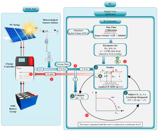
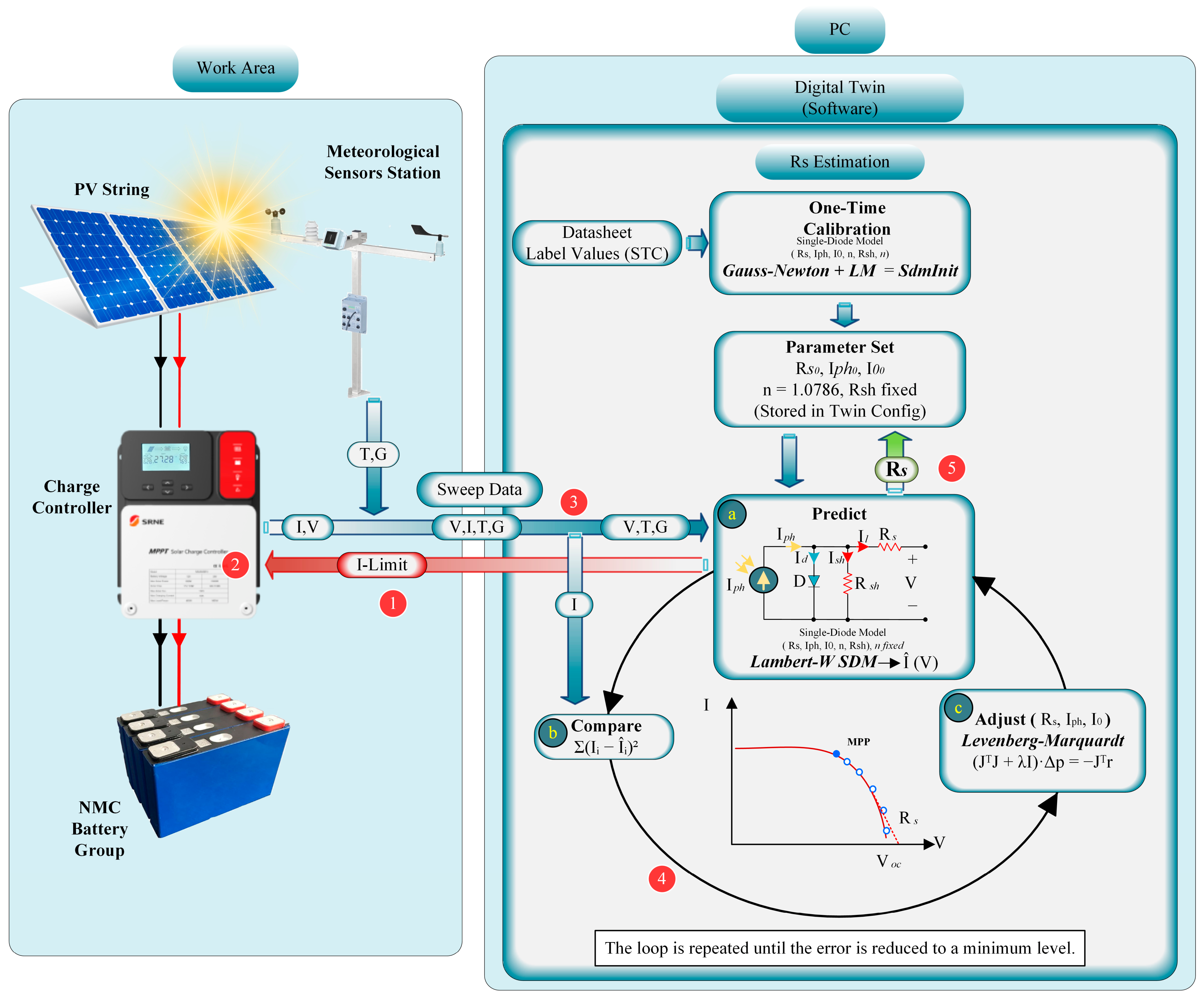
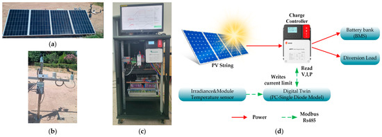
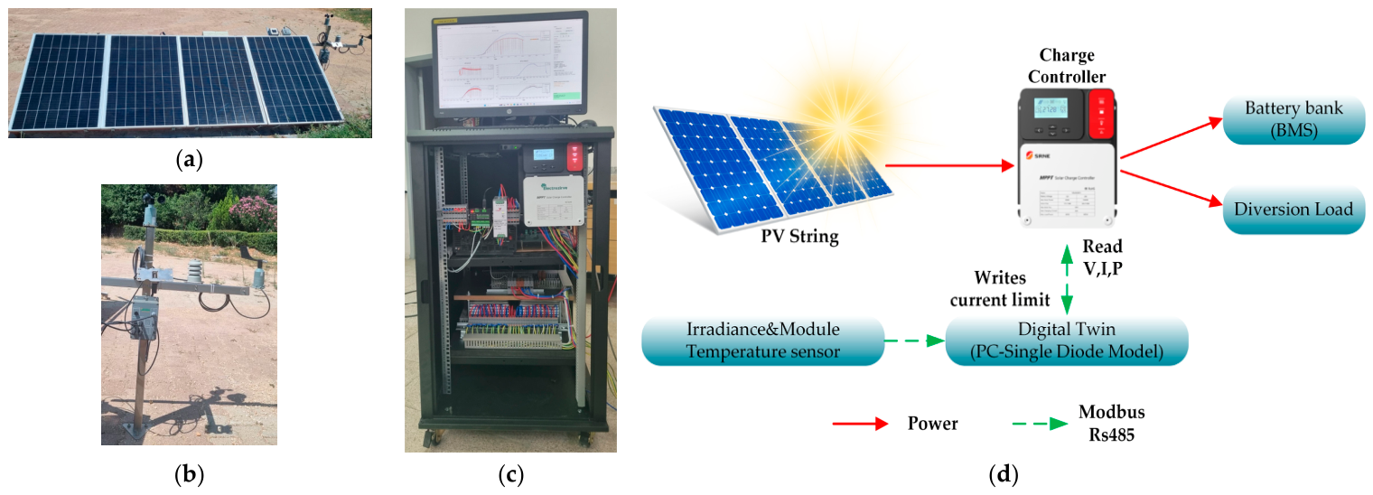
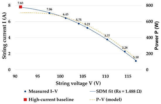
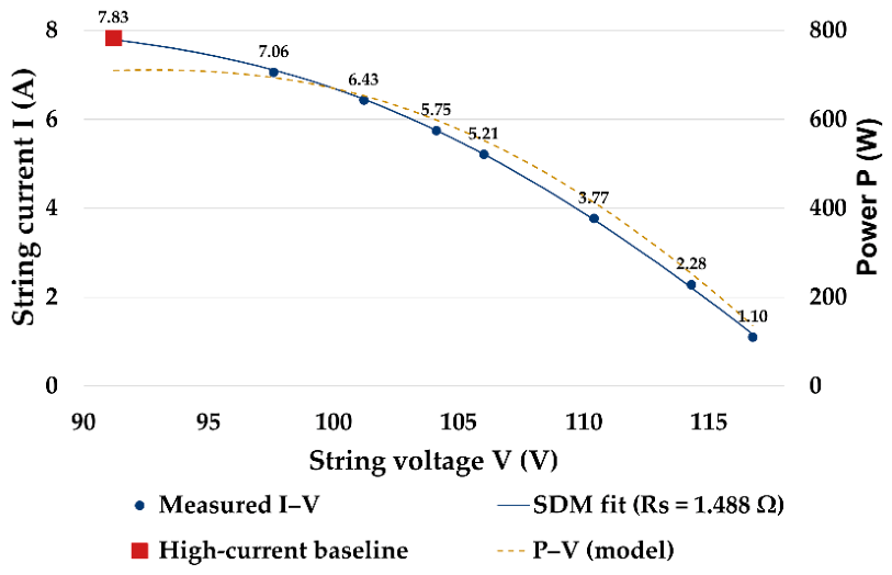
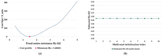
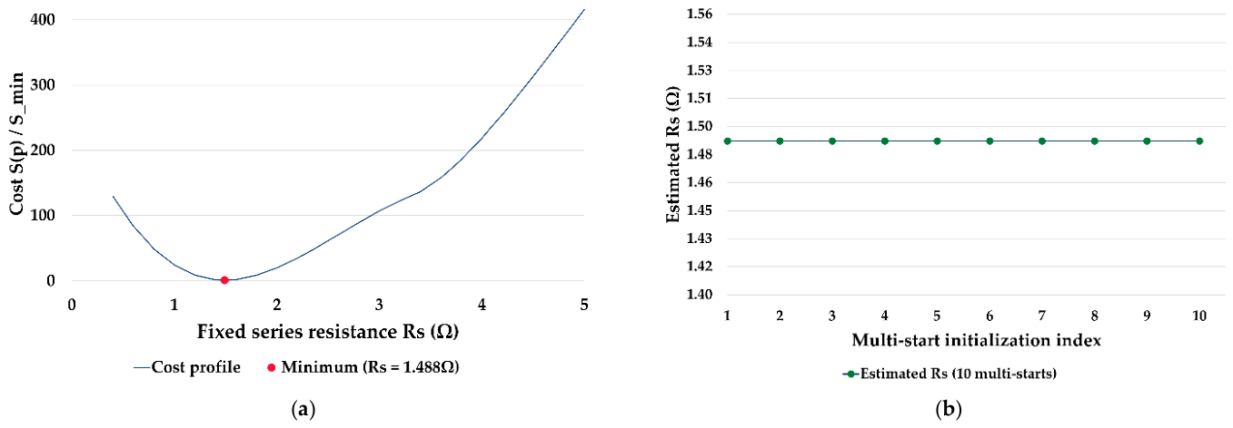
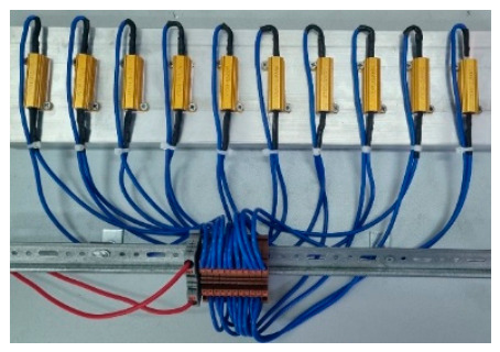
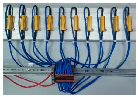
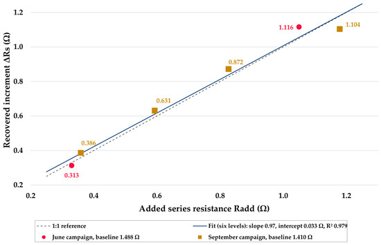
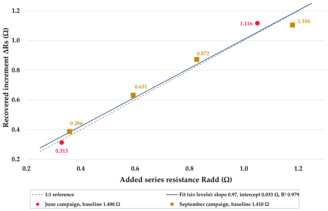
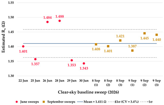
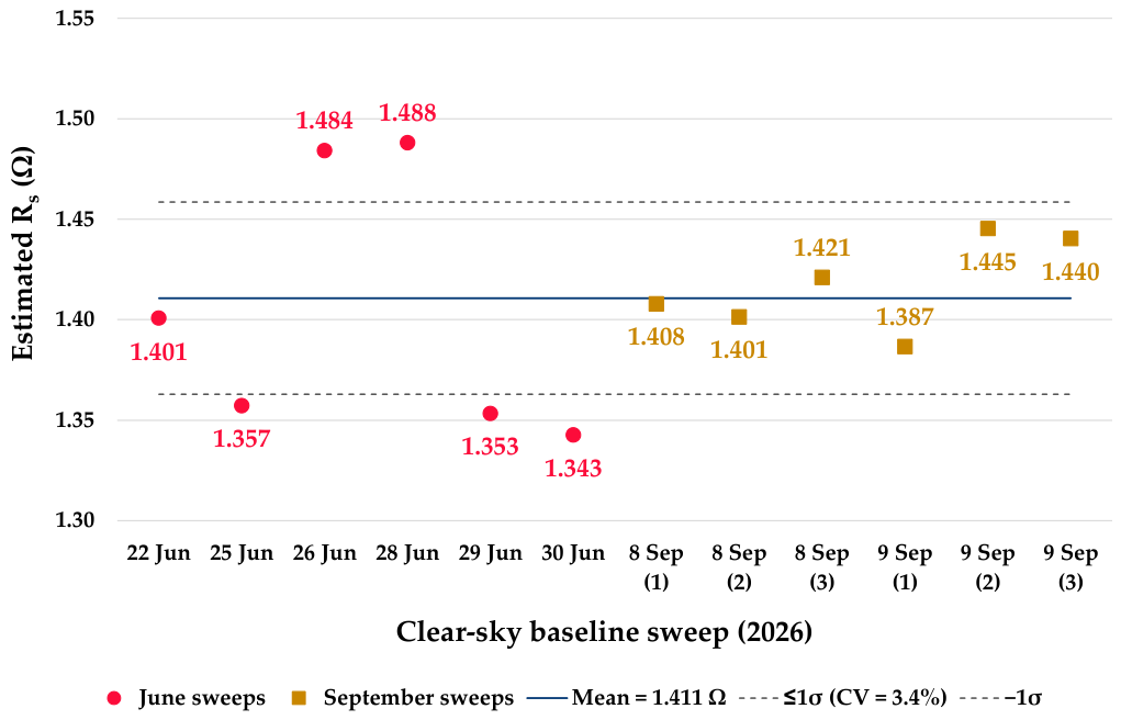

Disclaimer/Publisher’s Note: The statements, opinions and data contained in all publications are solely those of the individual author(s) and contributor(s) and not of MDPI and/or the editor(s). MDPI and/or the editor(s) disclaim responsibility for any injury to people or property resulting from any ideas, methods, instructions or products referred to in the content. |
© 2026 by the authors. Licensee MDPI, Basel, Switzerland. This article is an open access article distributed under the terms and conditions of the Creative Commons Attribution (CC BY) license.