Innovative Cyber-Physical/Electronic AI-Assisted Digital Twin Model of Small Energy Harvesting Cantilever Power Generators

Abstract

The paper deals with the design of a Digital Twin model of an energy harvesting cantilever beam for low frequency energy harvesting applications and specifically with a digital model matching simulations corresponding with Finite Element Method solutions in order to validate the model. The physical behavior is based on the main parameters to be investigated. The finite elements analysis is geometrically and parametrically carried out for a small PZT5A device of the orders of millimeters and is optimized to take into consideration the relationships between tip displacement, generated voltages and vibration gravitational forces for standard industrial applications in the acceleration range between 0.5 and 2 g. Then a procedure to integrate the Digital Twin into a design framework has been developed, including an artificial intelligence algorithm that supports the modelling of the real behavior of the device. The paper is devoted to help researchers involved in a Digital Twin adoption in the field of electronic design and of the physical characterization of low frequency energy harvesting devices exclusively using open-source tools.

1. Introduction

Piezoelectric cantilever beams having dimension within the millimeter and sub-millimeter range are used as small energy harvesting generators. Existing cantilever models take into account the physical oscillation behavior due to an excitation force [1] which can be either a pure sinusoidal signal (ideal case), or a damped wave (damping effect due to the air friction), or an irregular signal as for wind or ocean wave forces [2]. Different studies are addressed on the optimization of the model matching the mechanical and the electronic behavior by means an electromechanical model composed by transformers and diodes in bridge configuration [3,4,5]. These studies suggest the electronic elements to consider for a correct design of cantilever system generating an output power also considering different layouts as for ring-type devices increasing the generated power at low vibration frequencies [6]. Hardware equipment tools suitable for measurement approaches are constituted mainly by a controlled vibrating system (shaker or vibrating engine), a mechanical holder connected to the vibrating systems and to the electrodes reading the transduce signal, and a lock-in amplifier able to detect weak signals buried by high background noise by measuring the amplitude and phase of a resonant signal [6]. A tool that shows good potential for the cantilever design is the Finite Element Method (FEM) multi-physics software. In this direction, the open source FreeFEM tool [7] is suitable to numerically characterize piezoelectric devices [8,9,10,11]. Some studies combine the FEM multi-physics approach with SPICE based circuit simulations to model the charge readout circuit [12]. LTSpice open-source tool is applied in literature to solve piezoelectric problems addressed on energy harvesting applications [12,13,14,15]. An innovative approach to characterize piezoelectric energy harvesting devices is the formulation of a Digital Twin (DT) model including electronic design, FEM simulations and Artificial Intelligence (AI) data processing. Some authors studied DT to model predictive behaviors of piezoelectric materials implementing machine learning algorithm [16,17,18,19]. The DT models are mainly focused on a specific analysis, and not to the construction of primary cyber-physical model determining design requirements of piezoelectric energy harvesting devices. The proposed model is related to a small cantilever beam behaving as free-standing energy harvesting transducer generating electrical powers in micro-scales due to vibration forces. By focusing the attention on a basic structure of energy harvesting power generation such as cantilever beam in millimeter and sub-millimeter scale [20,21], the proposed study defines a methodological approach to construct a DT model suitable for the device design, by estimating frequency efficiency conditions and piezo-mechanical characteristics. Specifically, the paper is focused on discussing:

• the analytical equations describing the main piezoelectrical and mechanical properties of the cantilever;
• the SPICE-based model defining the electronic components of the whole vibrating system under vibration forces working at low frequencies;
• the Finite Element Method (FEM) supporting the device design including mechanical and piezoelectric simulations and describing the cyber-physical model of a common Lead Zirconate Titanate (PZT)-based cantilever (typical material used for vibration energy harvesting applications [22,23,24]);
• a protocol [25] defining the procedure to integrate DT model into a design framework discussing an example of AI application able to classify and clean a noisy signal [26,27] (see Section 4.2).

The proposed paper highlights the methodology to apply different digital technologies such as circuit simulators (Section 3.1), FEM simulators (Section 3.2) and AI data processing (Section 4.2) in order to structure a full design framework of cantilever beam energy harvesting systems.

2. Materials and Methods: Digital Twin Modelling

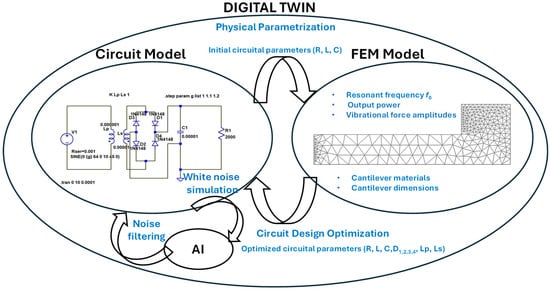
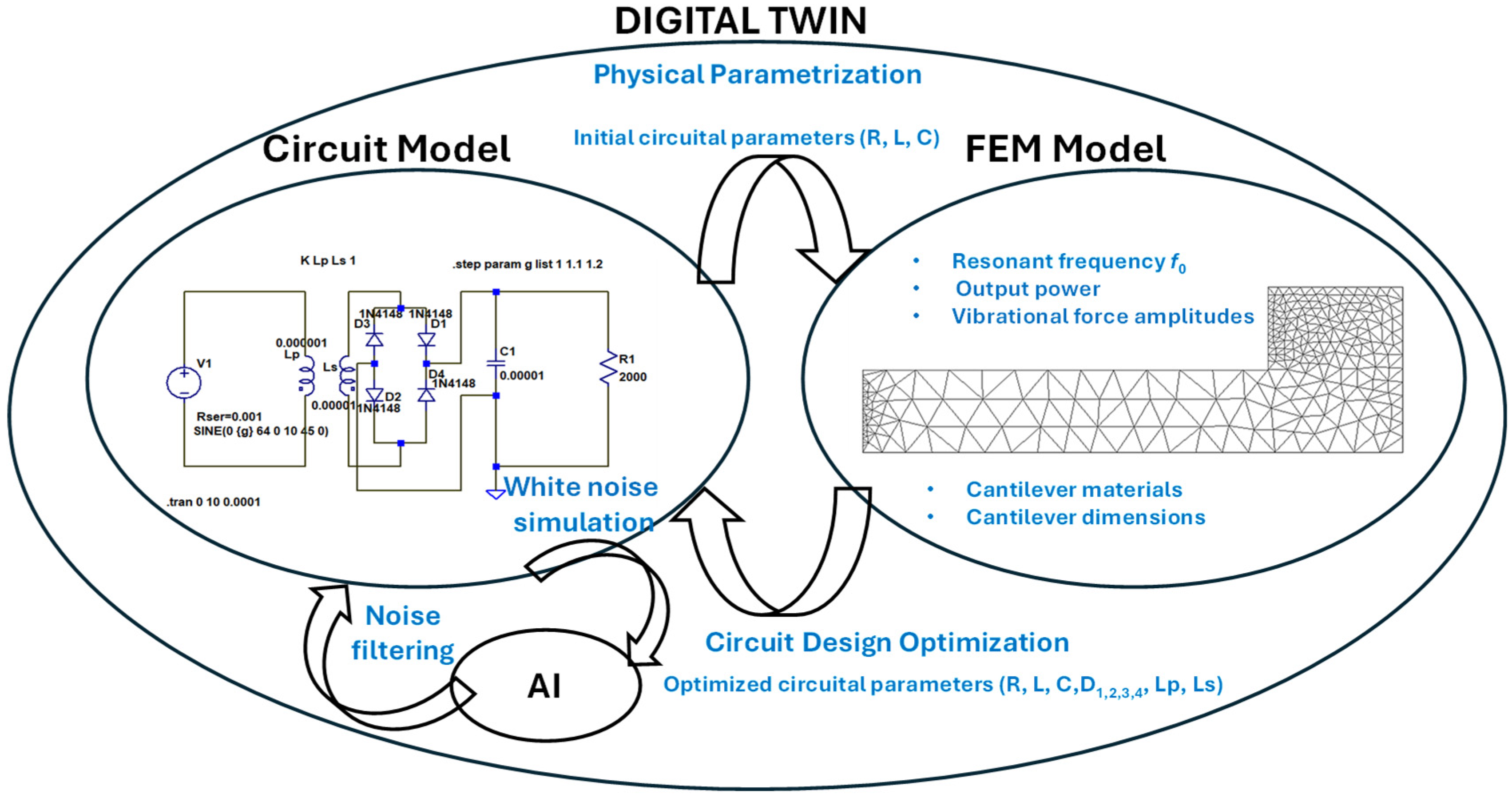
The proof of concept of the proposed DT model is sketched in Figure 1. The DT is based on the combined simulations of the SPICE-based electronic circuits and of the corresponding FEM physical structure to characterize mechanically and piezoelectrically the device. The proposed model defines the equations solved by the FEM simulator and the corresponding circuit providing the electrical output of the whole electronic circuit of a cantilever power generator under vibration forces. The analyzed DT is able to model the transduction of the mechanical energy enabled by vibration forces into electrical power: while vibrating, the cantilever beam generates by means of its piezoelectric properties of current and voltage outputs to be read by a circuit connected to two electrodes embedded in its structure. The geometrical parameters and the selected piezoelectrical material characterize the resonant frequencies (named as resonant modes) generating the higher electrical powers. The best efficiency of the cantilever beam is therefore obtained for vibration force frequencies corresponding to the resonant frequencies. Specifically, the DT integrates three tools: a FEM simulator, a Spice-based circuit simulator and an AI algorithm. These three tools are matched following the scheme of Figure 1 where the circuit model provides preliminary parameters such as resonant frequencies, circuital elements transferring the electrical power to a load, and a first idea of the time-domain and frequency-domain behavior of the cantilever beam. Successively, by means of matching the electrical outputs, the FEM provides information about the geometrical layout and the piezoelectric material to be applied. In addition, FEM simulations are important to find the best DT circuit parameters able to match its physical behavior. As a supplementary analysis, by processing the training model dataset, the AI is driven to classify and predict a real behavior of a noisy environment, after a signal cleaning so that the outputs are easy to read.

Figure 1. DT proof of concept including circuit design, FEM modelling and AI data processing.

The open-sources tools used for the modelling and simulations are: LTSpice (circuit simulations), FreeFEM (FEM simulations), and Konstanz Information Miner (KNIME) for AI data processing. The FEM model behaves as a proxy model approximating input-output relationships of the real physical structure, and providing a reliable predictions of the electro-mechanical behavior.

All simulations have been run by using a Intel Core i5 2.4 GHz/16 GB RAM processor.

Analytical Model of the Cantilever Beam Structure

The FreeFEM open-source tool implements the time-harmonic piezoelectric library. The solved equation takes into account the following relationship in circular coordinate system between the displacement u(t), the stress tensor T, the strain tensor S, the electric displacement field D, and the electrical field E:

$$\left[\begin{array}{c}\begin{array}{c}{T}_{rr}\\ T_{\theta \theta }\\ T_{zz}\end{array}\\ T_{rz}\\ D_r\\ D_z\end{array}\right]=\left[C\right]\left[\begin{array}{c}\begin{array}{c}{S}_{rr}\\ S_{\theta \theta }\\ S_{zz}\end{array}\\ S_{rz}\\ E_r\\ E_z\end{array}\right]$$

(1)

with [8]

$$\left[C\right]=\left[\begin{array}{cccccc}{c}_{11}& c_{12}& c_{13}& 0& 0& -e_{31}\\ c_{12}& c_{11}& c_{13}& 0& 0& -e_{31}\\ c_{13}& c_{13}& c_{33}& 0& 0& -e_{33}\\ 0& 0& 0& c_{44}& -e_{15}& 0\\ 0& 0& 0& e_{15}& {\epsilon }_{11}& 0\\ e_{31}& e_{31}& e_{33}& 0& 0& {\epsilon }_{11}\end{array}\right]$$

(2)

and

$$\left[\begin{array}{c}\begin{array}{c}{S}_{rr}\\ S_{\theta \theta }\\ S_{zz}\end{array}\\ S_{rz}\\ E_r\\ E_z\end{array}\right]=\left[\begin{array}{c}\begin{array}{c}{\displaystyle \frac{\partial }{\partial r}}{u}_r\\ {\displaystyle \frac{1}{r}}{u}_r\\ {\displaystyle \frac{\partial }{\partial z}}{u}_z\end{array}\\ {\displaystyle \frac{\partial }{\partial r}}{u}_r+{\displaystyle \frac{\partial }{\partial z}}{u}_z\\ -{\displaystyle \frac{\partial }{\partial r}}\Phi \\ -{\displaystyle \frac{\partial }{\partial z}}\Phi \end{array}\right]=L\left(\left[\begin{array}{c}{u}_r\\ u_z\\ \Phi \end{array}\right]\right)$$

(3)

being c_ij the elastic coefficients, e_ij the piezoelectric coefficients, ε_ij the dielectric coefficients, Φ a scalar function (in the proposed model is the voltage potential of the cantilever electrodes), and L() is a derivative operator. For the time-harmonic case T, S, D and E, the equation solving the variables of displacement is the following Equation [23]:

$$-{\omega }_0^2\rho u_i=T_{ij,j}{D}_{i,i}=0$$

(4)

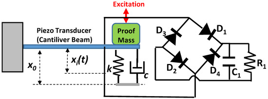
The movement of the piezoelectric cantilever beam is described by the following simplified equation representing the current flowing in the circuit of Figure 2 and the cantilever displacement u(t) = x(t) [1]:

$$i\left(t\right)={\displaystyle \frac{\alpha du(t)}{dt}}-C_p{\displaystyle \frac{di(t)}{dt}}$$

(5)

$$ku\left(t\right)=F\left(t\right)-\alpha i\left(t\right)-c{\displaystyle \frac{du(t)}{dt}}+M{\displaystyle \frac{d^{2}u(t)}{d{t}^2}}$$

(6)

with i(t) is the current generated by the vibrations and flowing in the circuit of Figure 2, and:

Figure 2. Cyber-physical model of a micro piezoelectric cantilever generating an output power due to a vibration excitation (excitation force): k is the spring constant c is the damping factor.

• α = e₃₃ A/L is the electromechanical coupling factor linked with the e₃₃ piezoelectric coefficient, being A and L are the cantilever surface and length, respectively;
• C_p = ε₃₃ A/l is the clamped capacitance of the piezoelectric element expressed in C/V (ε₃₃ is the elasticity coefficient, and l is the cantilever thickness);
• k is the spring stiffness of the cantilever, which for a uniform beam is (3·E·I)/L³, where E is Young’s modulus and I is the area moment of inertia;
• M is the total mass provided composed by the sum of the proof mass and the cantilever one;
• F(t) = F₀ sen(2πf₀t) is the excitation vibration force (force factor) characterized by an oscillation frequency of f₀;
• c is the damping factor modelling all the mechanical losses.

The equation model of Equations (5) and (6) indicates a simplified analytical model highlighting the physical effects. The numerical equation solved in the DT is represented by Equation (4) [8,23].

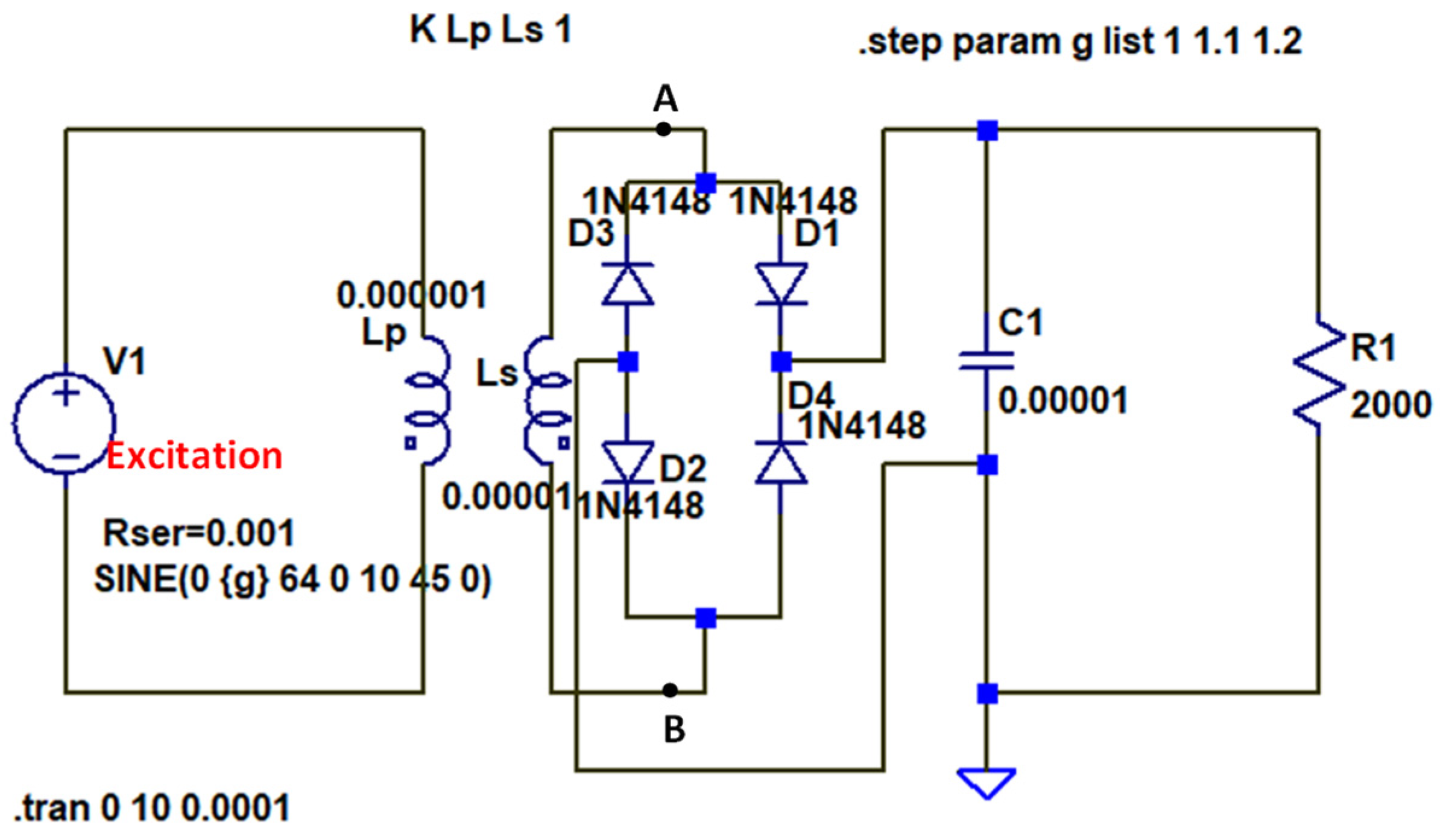
The piezoelectric-mechanical model of the cantilever beam is illustrated in Figure 2: the cyber-physical model is composed by the piezo transducer couple with a bridge rectifier connected to two surfaces of the cantilever beam (typically constituted by thin metallic layers [6]) composed by four diodes (D1, D2, D3 and D4 of Figure 2) and by a resistance and capacitive RC circuit transferring the generated electrical power to a load transforming the alternate current signal into a direct current one. Lumped element modeling is a versatile technique, that requires careful consideration of component accuracy, interconnect effects, and validation with measurements. The adoption of the lumped elements in the proposed allows a preliminary design. The FEM approach is applied in this work to optimize and validate the choice of the whole electrical and electronic components simulating their physical behavior.

3. Results

The results proposed in this section are related to circuit and FEM simulations.

3.1. Circuit Modelling and Simulations

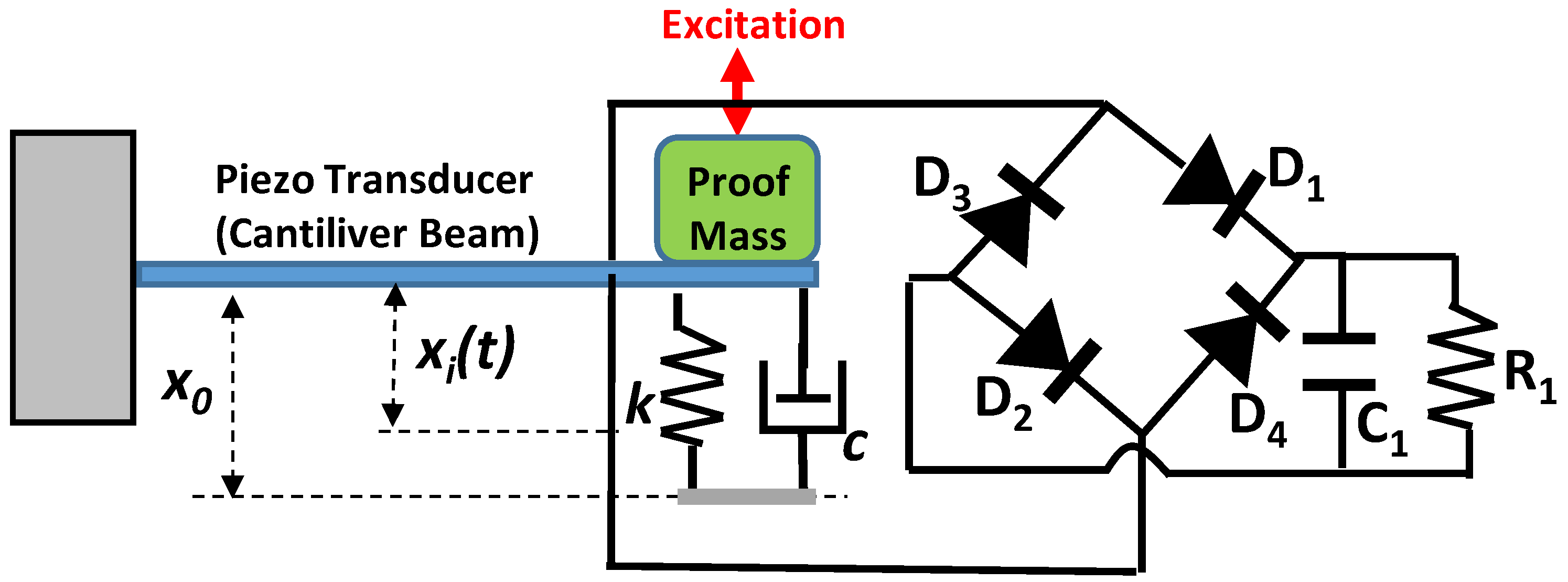
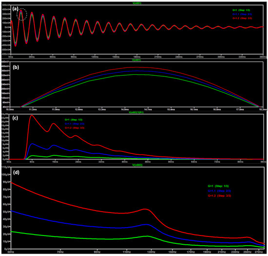
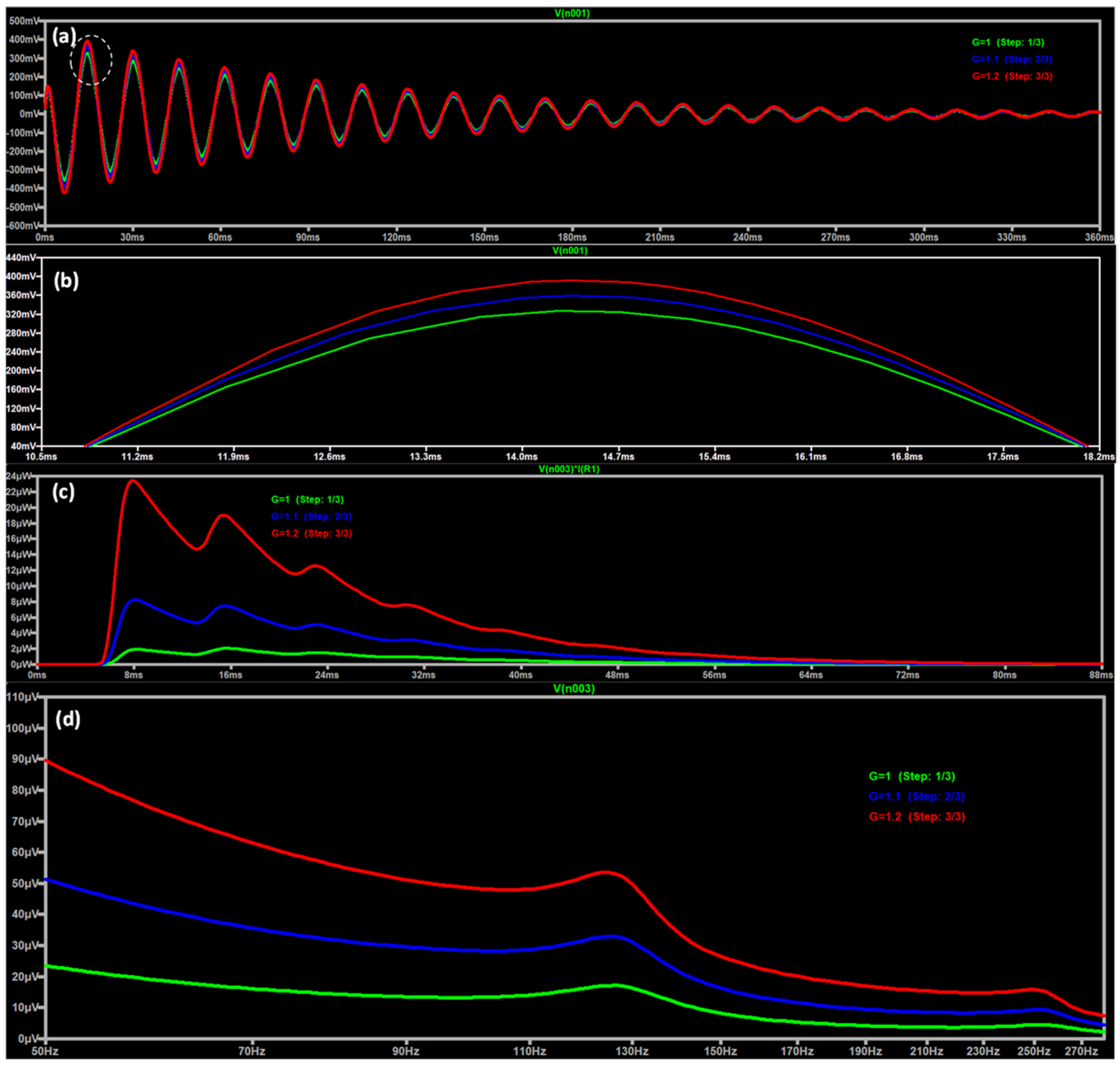
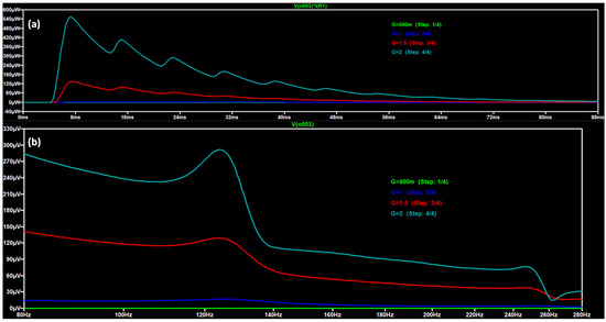
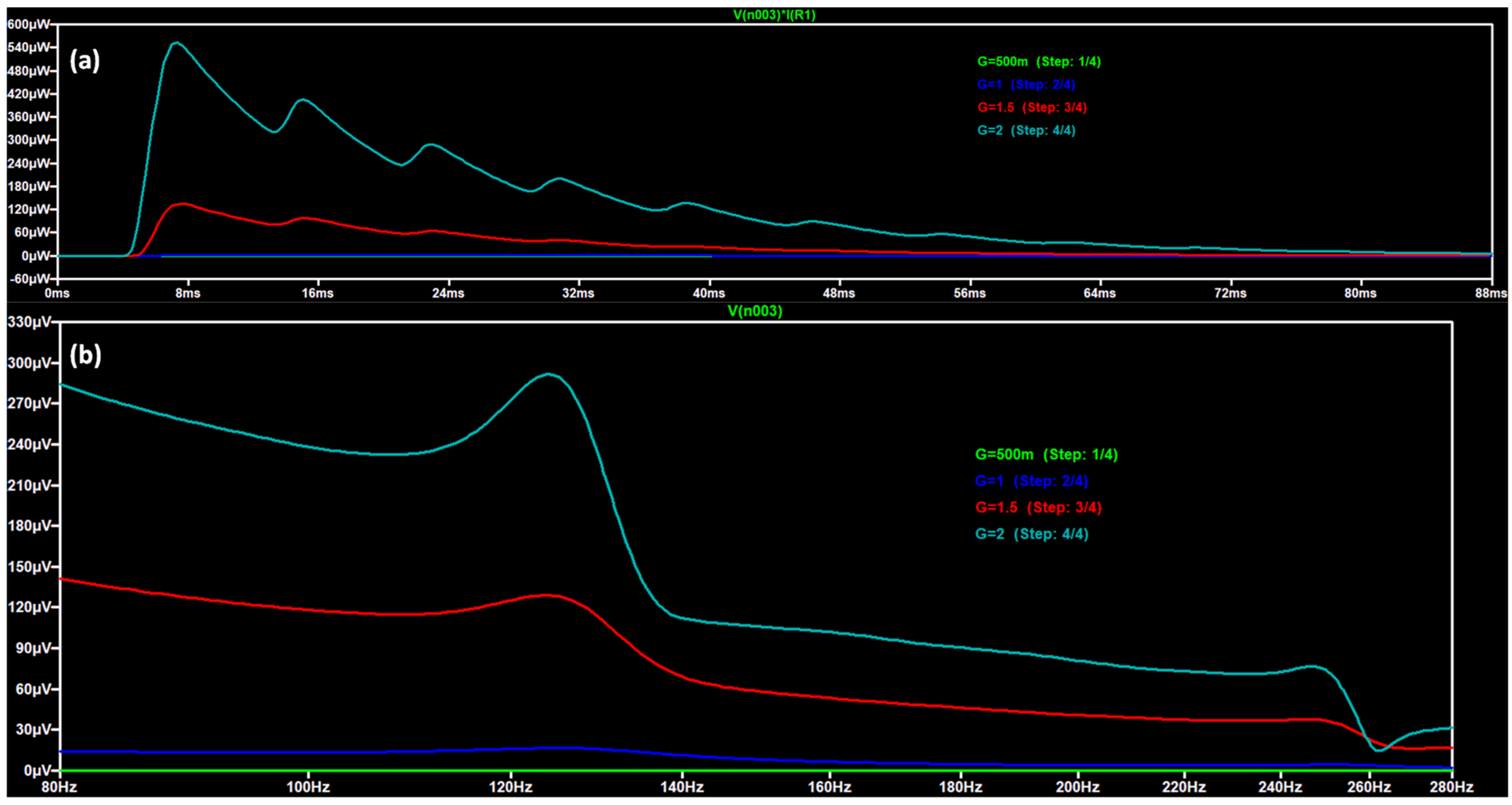
The circuit model is constructed by means of LTSpice (Version x64 24.1.8), an open-source SPICE-based electronic circuit simulator computer software. The circuit model is built up for a parametric analysis to describe the output power trend changing the excitation force amplitude. Specifically, the proposed circuit model in Figure 3, is implemented by the LTSpice tool using a low excitation frequency of f₀ = 64 Hz (as used in literature for experimental setups [6]), a bridge of diodes (1N4148 type) rectifying the signal, and by a resistance and capacitance RC circuit transferring the electric generated power to a load (R1 resistance). The analytical model of the cantilever beam is ‘translated’ by the LTSpice circuit of Figure 3 solved by the Kirchhoff equations providing the electrical current and voltage in each node of the simulated circuit. The mechanical vibration forces are modelled by the analogic voltage generator [24] (V1 generator) as sinusoidal force exciting the structure with an operating frequency of 64 Hz and implementing parametrically different accelerations. Figure 4a,b illustrates the input electrical signal modelling the time-domain vibration dumped force acting at the low frequency of f₀ = 64 Hz (example of frequency used in experimental setup [6]) for different acceleration values (1 $\mathrm{g}$, 1.1 $\mathrm{g}$ and 1.2 $\mathrm{g}$). Figure 4c and Figure 4d show the parametric time domain output power V_R1·I_R1 and the output spectra (Fast Fourier Transform -FFT- of the V_R1 voltage signal), respectively. The parametric analysis is successively performed on the whole range of industrial vibration forces for accelerations ranging from 0.5 $\mathrm{g}$ to 2 $\mathrm{g}$ [6] (see Figure 5a,b). All the analysed spectra prove the presence of a resonant frequency (eigenfrequency) near 125 Hz (the eigenfrequency varies from 124. Hz to 125.6 Hz for accelerations ranging from 0.5 $\mathrm{g}$ to 2 $\mathrm{g}$) due to the RLC behavior of the whole circuit (pass band behavior cantered to the harmonics being multiples of a fundamental working frequency, also called the first harmonic). By observing the spectra of Figure 4d it is evident that for vibration frequencies near 64 Hz the voltage output is slightly higher if compared with the same signal at 125 Hz. In any case, the choice of frequencies close to 125 Hz is due to what happens in industrial environments that is that different types of machinery show different vibration signatures at this frequency (noise frequency most likely to be found in industrial applications). Mechanical resonance occurs when the frequency of an external force coincides with the natural frequency (eigenfrequency) of the cantilever (in our case 125 Hz), causing it to oscillate in an amplified manner. The natural frequency of a cantilever is the frequency at which it vibrates freely without external forces, or its natural frequency. It is an intrinsic property of the cantilever and depends on its mass, stiffness, and geometry. When the cantilever is “excited” by an external force (in our case at 64 Hz), it will begin to vibrate at its natural frequency. If the mechanical vibration frequency coincides with the natural one (as for common industrial vibration phenomena at 125 Hz), mechanical resonance occurs, a phenomenon that causes an extreme amplification of vibrations. Furthermore, Figure 4d shows the presence of a second resonant frequency near 250 Hz. The analysis will be focused on the first eigenfrequency characterized by a higher output power.

Figure 3. Equivalent electronic LTSpice circuit of the model of Figure 2 coupled with the surfaces of the cantilever beam structure (C1 = 0.01 mF and R1 = 2000 Ω).

Figure 4. LTSpice parametric analysis: (a) excitation signals of vibrational forces with different acceleration values (1 $\mathrm{g}$, 1.1 $\mathrm{g}$, 1.2 $\mathrm{g}$) and the damping effects. (b) Zooming of the voltage signal marked by the white dashed line in (a). (c) Time domain parametric output power simulated for different excitation forces. (d) FFT responses highlighting a working frequency near 125 Hz for a vibration acceleration of 1.2 $\mathrm{g}$.

Figure 5. Parametric analysis: (a) Spectra estimated for different accelerations 0.5 $\mathrm{g}$, 1 $\mathrm{g}$, 1.5 $\mathrm{g}$ and 2 $\mathrm{g}$ and (b) related FFT responses highlighting a working frequency near 125 Hz.

3.2. FEM Modelling and Simulations

The FEM model is implemented in FreeFEM tool (Release 4.13), a high level multiphysics finite element software solving constrained optimization problems solving Partial Differential Equations (PDE). The modelling and simulations are performed by characterizing the mechanical and piezoelectric behavior of the cantilever beam having a proof mass on the tip typically adopted to decrease the resonance frequency. The goal of the FEM simulations is to find a possible physical layout corresponding to the circuit of Figure 3 working at the resonance frequency of f₀ =125 Hz and completing the DT model combining physical and electronic design. The simulation is carried out by considering a geometrical parametric analysis to characterize the free-standing structure about the tip displacement amplitude and the generated voltage varying the accelerations from 0.5 $\mathrm{g}$ to 2 $\mathrm{g}$ as for circuit simulation. In Table 1 all the parameters adopted for the FEM simulation are listed considering a piezoelectric PZT5A material with a proof mass of the same material (mass added on the cantilever’s tip).

Table 1. Geometrical, mechanical and piezoelectric parameters adopted of the simulation of the PZT5A cantilever beam. The geometrical parameters are related to the performed analysis, mechanical and piezoelectric parameters are found in [8].

Geometrical Parameter	Value
Cantilever length a	a = 6 mm, a = 8 mm, a = 10 mm
Cantilever thickness l	l = a/6
Proof mass height wi	wi = a/6
Proof mass width po	po = a/4
Mechanical Parameters (PZT5A) [8]	Value
Young’s modulus E	5.5 GPa
Material density ρ	7750 kg/m3
Posson ratio v	0.31
Elastic coefficients cij	c11 = 120 × 109; c12 = 75.2 × 109; c13 = 75.1 × 109; c33 = 110 × 109; c44 = 21.1 × 109
Piezoelectric Parameters (PZT5A) [8]	Value
Piezoelectric coefficients eij	e31 = 5.4; e33 = 15.8; e15 = 12.3
Dielectric coefficients εij	ε11 = 8.1× 10−9; ε33 = 7.3 × 10−9

The FreeFem elasticity library takes into account the solution of equations of a solid deformation due to an applied force: each point of the cantilever structure, originally at the (x, y, z) position will come to (X, Y, Z) one after some time steps; the displacement vector is defined as u = (u₁, u₂, u₃) = (X − x, Y − y, Z − z). For small displacements and elastic solids, Hooke’s law gives the following relationship between the stress tensor σ_ij(u) and the strain tensor s_ij(u):

$${\sigma }_{ij}(u)=\lambda {\delta }_{ij}\nabla ·\mathbf{u}+2\mathrm{\mu }{s}_{ij}(u)$$

(7)

where the Kroneker symbol δ_ij = 1 if i = j, 0 otherwise, with

$$s_{ij}\left(u\right)={\displaystyle \frac{1}{2}}\left({\displaystyle \frac{\partial u_i}{\partial x_j}}+{\displaystyle \frac{\partial u_j}{\partial x_i}}\right)$$

(8)

and where λ and μ are mechanical constants correlated with Young’s modulus E and the Poisson ratio ν by:

$$\mu ={\displaystyle \frac{E}{2(1+\nu )}}, \lambda ={\displaystyle \frac{E\nu }{(1+\nu )(1-2\nu )}}$$

(9)

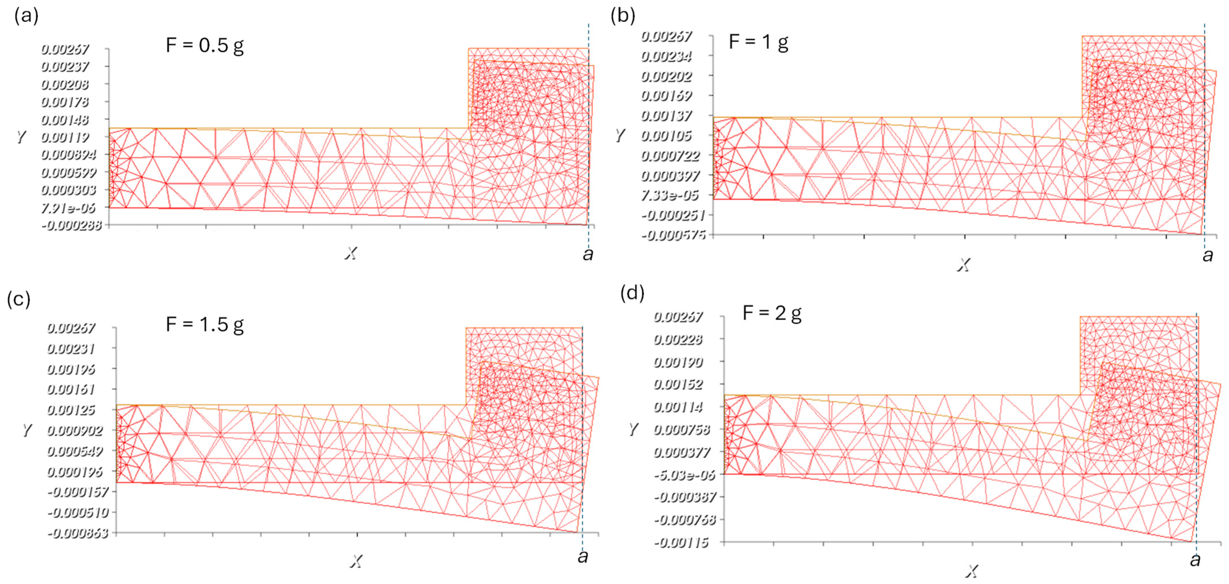
In Figure 6a–d is estimated the maximum FEM deformation u of the PZT5A cantilever structure for different accelerations ranging from 0.5 $\mathrm{g}$ to 2 $\mathrm{g}$.

Figure 6. (a–d) Simulation of the elastic behavior (u deformation) of the cantilever beam with proof mass by applying a vibration force with different accelerations (0.5 $\mathrm{g}$, 1 $\mathrm{g}$, 1.5 $\mathrm{g}$ and 2 $\mathrm{g}$). X and Y are the coordinates of the cantilever beam defining the 2D spatial domain.

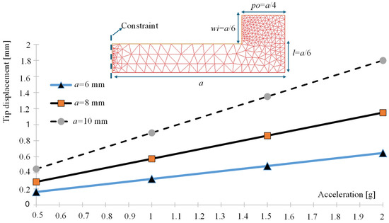
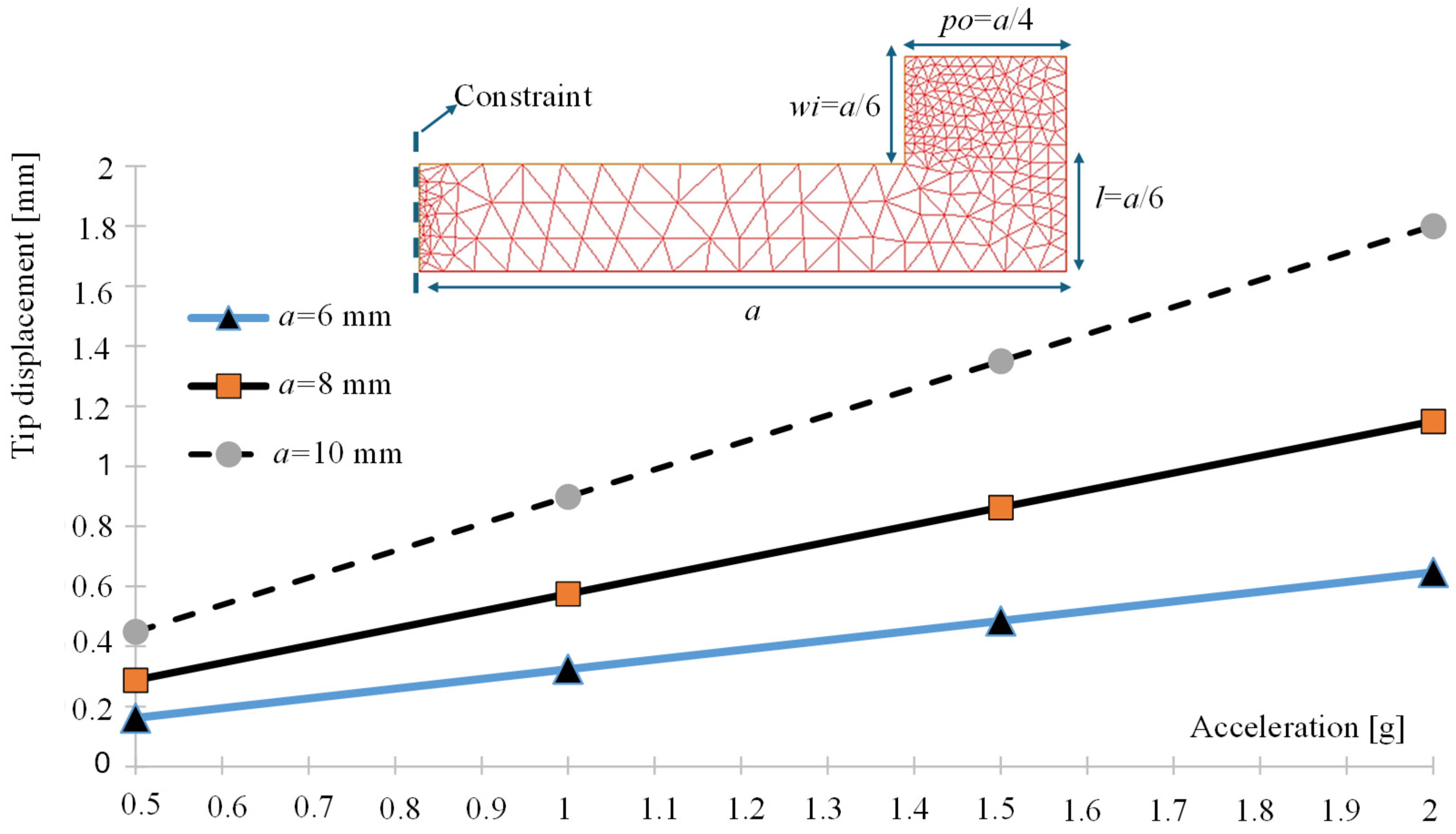
In Figure 7 are summarized the tip displacement trends versus the acceleration of the vibrational forces for different millimeter structures observing an increasing linear trend. As expected, the longer the cantilever, the greater major the tip displacement.

Figure 7. Tip displacement versus the acceleration of the vibrational force for different geometries of the cantilever beam in the millimeter scale. Inset: geometrical parametric model of the simulated piezoelectric device.

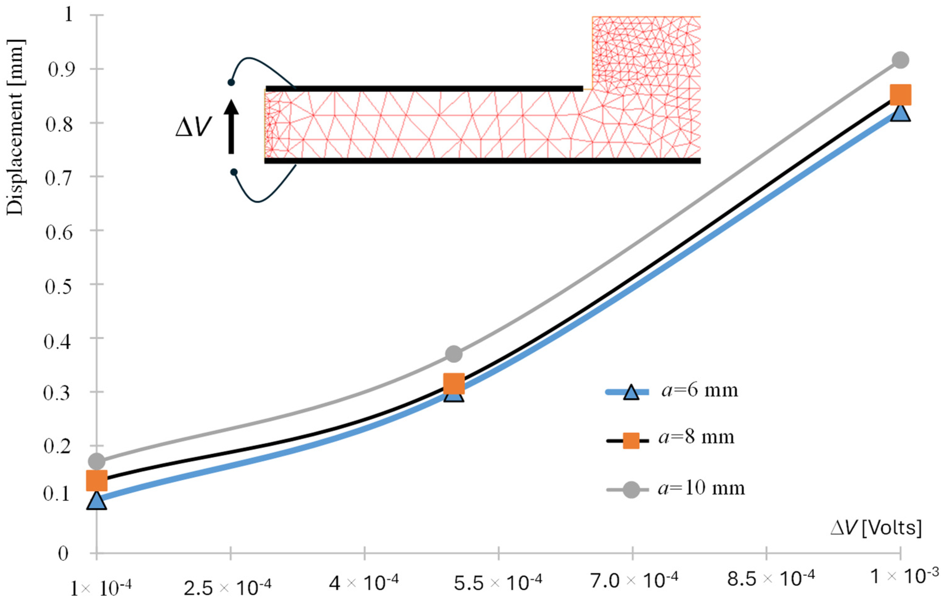
In order to characterize the relationship between the generated output voltage due to the vibrations and the maximum tip displacement, it is executed the FreeFEM Piezoelectric library setting as boundary condition the voltage variable Φ defining the variation of potential ΔV able to generate the electric current flowing in the circuit of Figure 3. In Figure 8 the relationship between the tip displacement and the generated ΔV is estimated for a cantilever working at a harmonic frequency of f₀ = 125 Hz (frequency estimated by the circuit simulation of Section 3.1): as expected the larger the tip displacement, the greater the potential difference ΔV.

Figure 8. Tip displacement versus the variation of voltage ΔV estimated on the cantilever surfaces as indicated in the Inset scheme (the black lines indicate the metallic boundary condition estimating the variable Φ).

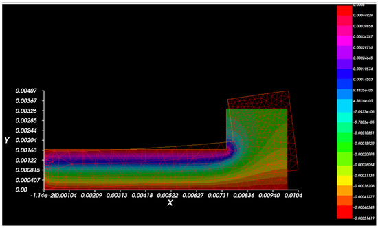
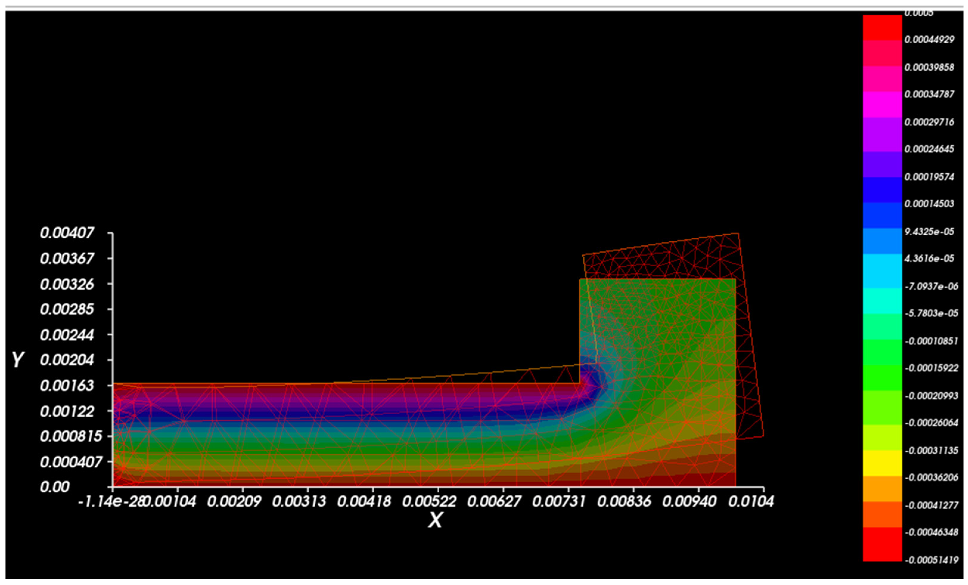
Figure 9 illustrates an example of the ΔV distribution in the whole structure for a maximum tip displacement of 0.916 mm. By comparing the voltage at the nodes A and B of circuit of Figure 3 with the estimated ΔV we conclude that the Simulation of Figure 9 corresponds to a transformer Lp = Ls = 1.78 × 10⁻⁶ H. The comparison of the circuit and the relevant FEM simulations allows to refine the parameters of the equivalent circuit, thus optimizing the whole design: the design starts with hypothetical parameters (as for Lp and Ls) and, successively, by means of the comparison of the estimated ΔV values, the circuit is set to be the very close DT of the physical model. According to the physical structure simulated by FEM a maximum output voltage of ΔV = 0.5 mV (see Figure 9) corresponding to a maximum tip displacement of 0.37 mm is able to fix the parameters Lp and Ls (corresponding to Lp = Ls = 1.78 × 10⁻⁶ H) and, consecutively, to allow the correct matching between the circuit and the physical structure (matching of the vibrating source power).

Figure 9. FEM simulation: estimation of the ΔV distribution (HSV color scheme) for a cantilever with a = 10 mm for a maximum displacement of 0.916 mm. The color bar is in voltage units. X and Y are the coordinates of the cantilever beam defining the 2D spatial domain.

By comparing the simulated ΔV, calculated at the load of the circuit of Figure 3, with the FEM ΔV values, is obtained the matching between the physical structure and the Lp and Ls values (see Table 2) which defines the equivalent input voltage.

Table 2. Matching between FEM output voltages and Lp and Ls circuit parameters fixing the geometrical parameter a = 10 mm and the acceleration equals to 1 $\mathrm{g}$.

FEM Piezoelectric ΔV [mV]	Maximum Tip Displacement [mm]	Lp, Ls [H] (Lp = Ls)
0.1	0.17	0.95 × 10−6
0.5	0.37	1.48 × 10−6
1	0.9	1.78 × 10−6

4. Discussion: DT Protocol and AI Improvement

4.1. BPMN Protocol of DT Implementation

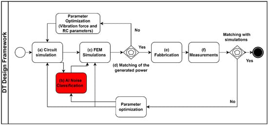
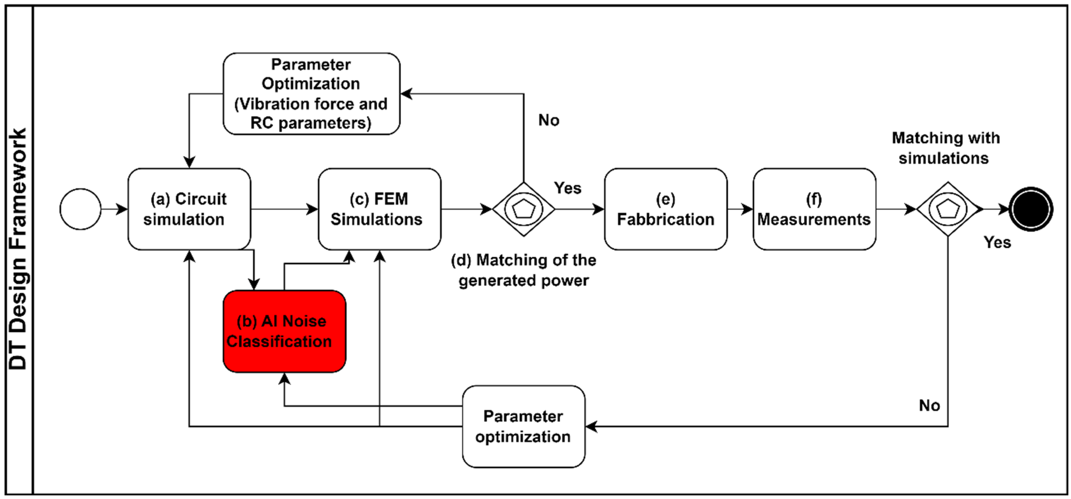
The Business Process Modelling and Notation (BPMN) graphical approach is a standard notation (ISO/IEC 19150:2013) typically adopted to formalize protocols and procedures as for measurements of nano-devices [25]. In this section, the BPMN workflow of Figure 10 illustrates a procedure to define a complete DT framework for the design of energy harvesting design by the following stages:

Figure 10. BPMN workflow defining the framework of the DT design framework.

• Stage (a): circuit simulation providing information about relationship between output power and working frequencies defining electronic components (diodes, resistances, capacitances, etc.) generating the power output;
• Stage (b): AI algorithms simulate real behaviors introducing circuit noises; the AI classification is also useful to classify the measurements by distinguishing the noise from the true signal; the feedback loop allows to consider for the AI simulation the correct circuit parameters obtaining a more precise noise modelling and, consecutively, a more realistic reconstruction of the clean signal;
• Stage (c): FEM piezoelectrical and mechanical simulations providing a physical model and fixing geometrical and circuit parameters comparing the FEM output voltages with the circuit ones;
• Stage (d): the matching between the estimated FEM power and voltage with the SPICE ones will define the optimized components, otherwise will be changed the electrical values and the circuit parameters (as for the transformer modelling the power transfer of the vibration excitation signal of the input voltage generator);
• Stage (e): fabrication of the optimized device;
• Stage (f): measurements are suitable to provide a further validation of the DT model supporting the parameter optimizations by means of the comparison between numerical and experimental results.

The methodology applied for the parametric optimization is summarized in the following steps:

(1)

An initial circuit is designed and simulated (Spice simulation) to find good output performance about power conversion and analyzing the main resonant frequencies starting to a specified vibrating force characterized by a specific working frequency: the initial model allows to fix some circuit elements and parameters (see Figure 3) such as diodes (D1, D2, D3 and D4), transformer windings (Lp and Ls), the capacitance C1 and the load resistance R1. The initial circuit takes into account the modelling of the external vibration forces with physical information lumped into the voltage generator V1 (see Appendix A) embedding mass, damping and strain parameters (modelling of the physical parameters into a circuit ones).

(2)

Starting to a resonant frequency found in the circuit simulation, the FEM simulation is run to check the resonance by means the physical model. The check is performed by comparing mainly the output voltage of the circuit model of Figure 3 (voltage of the load R1) with the FEM cantilever beam structure for different vibrating accelerations and providing different output powers. The matching between the calculated voltages (both Spice and FEM) allows to optimize the circuit model of the vibration force and the other circuit parameters such as Lp, Ls, C1, R1 and D1, D2, D3 and D4. The parameter refinement provides an optimized circuit DT of the physical model: a precise circuit will correspond to a specific cantilever physical model fixing geometries and materials. The FEM model provides the parameters of the structure to fabricate.

(3)

The construction of a precise DT allows to analyze and classify possible noises which could be observed during experimentation: AI supports the cleaning of a possible noisy signal and, consecutively, the interpretation of experimental results characterized by a ripple trend of the output voltage (ripple due to the noise).

The parametric analysis varying acceleration provided more signals training the ANN network. The training model is constructed without the introduction of the white noise and considering the LTSpice calculated voltages with different accelerations to increase the training dataset dimension and to decrease the calculus error. The ANN compares the noisy signal (testing signal) with those of the training model thus classifying the signal most similar to those identified in the absence of noise and attenuating the ripple behavior. According with the workflow of Figure 10, the AI allows to adjust the circuit parameter by distinguishing the ideal model (ideal DT providing design parameters) from the real one (DT of the real scenario) affecting by noises. Consecutively, also the FEM setting will be calibrated by selecting the ideal case to provide the design specifications.

4.2. Example of AI Application

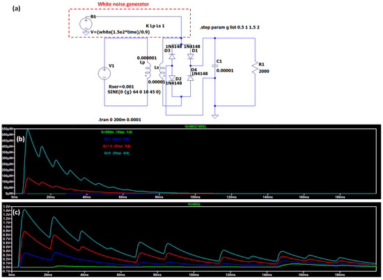
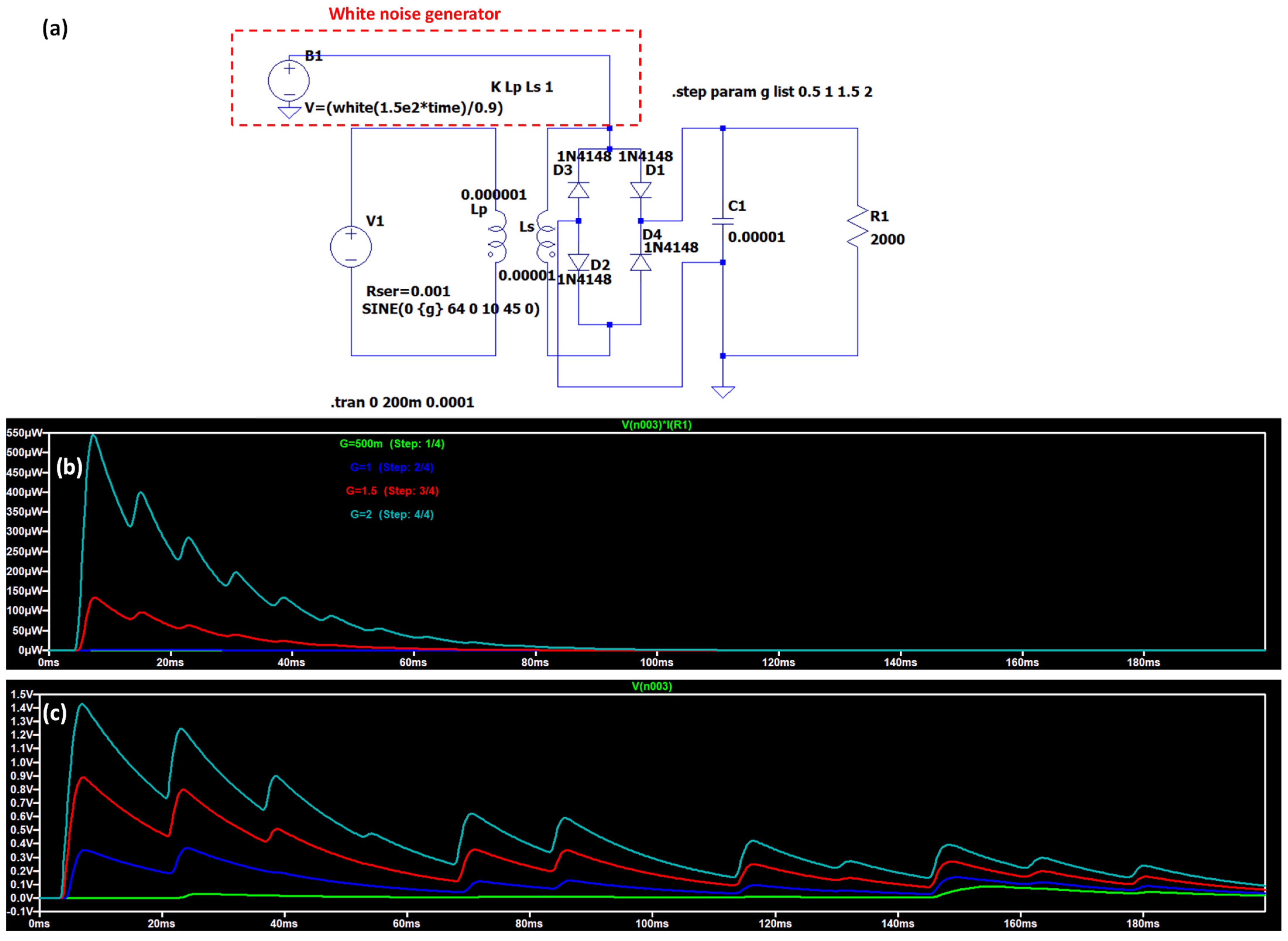
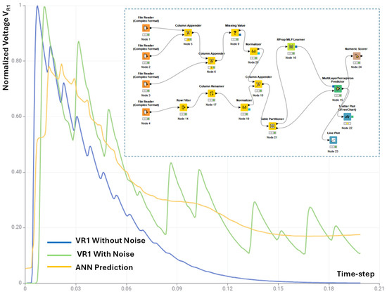
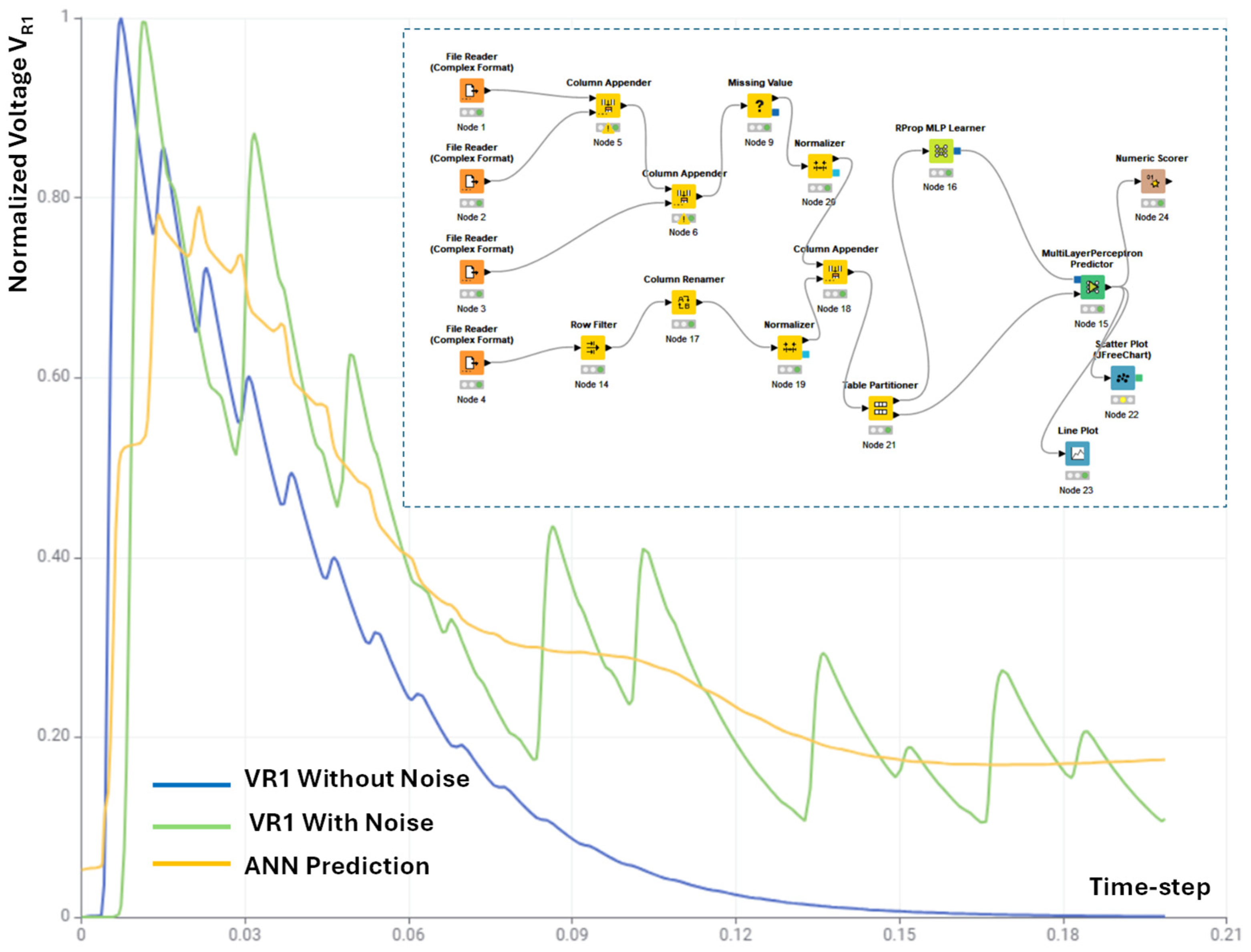
The AI data processing is a useful tool to classify a noisy signal [26], by cleaning the strong ripples covering the voltage output signal [27]. The undesired ripples are due to interferences or noises. As proven in [26,27], Artificial Neural Networks (ANNs) are good candidates to construct training models by circuit simulations and to process noisy electronic signals. ANN is applied in this work to show an example of AI data processing able to adjust a strong ripple signal due to a white noise signal. The white noise signal is typically adopted to simulate interferences or noises acting on an electronic circuit. The white noise is modelled by a voltage generator changing the voltage in specific node of the analyzed circuit (see Figure 11a) obtaining the voltage and the power signals of Figure 11b and Figure 11c, respectively (parametric analysis for different vibration forces). The output voltages of the circuit simulations are used to train the ANN network: the training is performed by means of signals without noise (3093 records of the voltage output V_R1 of the circuit without the white noise generator), besides the noisy signal is processed as testing signal (data refers to the output voltage of the simulated circuit of Figure 3, calculated on the load resistance R1 for the training and of the simulated circuit of Figure 11 for the testing). The example in Figure 12 proves the principle to clean and adjust a ripple signal due to a noise by means of ANN. In Table 3 the main performance parameters of the ANN for the optimized model (epochs number equals to 100, 1 hidden layer, number of neurons per layer equals to 10) are listed. The hyper-parameters of the ANN network are selected to minimize the calculus error. The MAE error of the 7% indicates a good performance of the algorithm.

Figure 11. (a) LTSpice circuit modelling white noise interferences. Output power (b) and voltage (c) signals disturbed by the white noise.

Figure 12. Comparison between the normalized output signal V_R1 (without and with the white noise interference) and the ANN prediction correcting the undesired ripple trend. Inset: KNIME workflow performing the ANN estimation. The time-step is associated to the record number of the analyzed dataset.

Table 3. ANN error statistical parameters for the optimized model obtained for epochs number equals to 100, 1 hidden layer, and number of neurons per layer equals to 10.

Error Parameter	Value
Mean Absolute Error (MAE)	0.07
Mean Squared Error (MSE)	0.011
Root Mean Squared Error (RMSE)	0.103
Mean Absolute Percentage Error (MAPE)	0.245

In the inset of Figure 12 is illustrated the KNIME (Version 5.5.2) workflow implementing the ANNs distinguishing the data input, the data pre-processing and the data processing stages. The ANN predicted signal allows to attenuate the noise ripples. For this reason the ANN network behaves as a ‘filter’ cleaning the noisy background and supporting the correct reading of the output by separating the noise effect from the useful signal. As Algorithm 1 is listed the pseudocode of the ANN implementation.

Below is listed the pseudocode of the ANN implementation:

Algorithm 1: Pseudocode of ANN implementation

1. Start training model construction; 2. Initial circuit parameter setting according with design specifications (offline training model construction); 3. If check of FEM results is positive Then save output voltage as training dataset (ideal signals) Until data are enough (training model optimization); 4. Else (negative check) execute other parametric analysis finding the best matching with FEM and therefore constructing the correct training dataset; 5. End If; 6. Construct the circuit noisy model (construction of testing dataset); 7. If the model reply the signal trend of experimental results Then fix the circuit parameters and save the simulated voltages for the ANN testing; 8. Else modify the noise modelling to reply the noisy ripple behavior Until the trend of simulated results is similar to the experimental one (selection of the final testing signal); 9. End If; 10. Execution of the ANN data processing optimizing the hyper-parameters. 11. Discrimination of the best real DT model from the ideal one.

The ANN model is also suitable to predict other signal characteristics including transient variations and harmonic distortions by constructing a training model with different time domain signals. The performance of the ANN tool is not comparable with the circuit and FEM performance as they are part of a supplementary analysis about signal cleaning. The ANN could be applied to adjust the experimental setup obtaining clean signals as predicted by the AI Kernel. This optimization is useful to optimize other numerical parameters of the FEM and Spice tools as well: matching between the ANN-clean signal profile with the experimental measurements obtained by optimized experimental setup is important to define correct numerical parameters with no variability issues.

4.3. Discussion About DT Novelties, Key Features and Limitations

Table 4 and Table 5 summarize the key features and the limitations of the proposed DT model.

Table 4. DT novelties and key features.

Work Novelties and Key Features	Discussion
DT tool integrating SPICE, FEM and AI tools (combined use of the three tools)	Possibility to model the whole energy harvesting system by checking physical, geometrical and circuital parameters by predicting possible measuring errors or disturbs.
Variability analysis	The model is suitable to define a validation range of all the circuital parameters by means the Monte Carlo and WCA approaches.
Protocol integrating the DT in a real scenario involving measurements (Figure 10)	The work proposes a protocol to integrate all the simulation tools into a procedure addressed to check the real behavior of the cantilever beam. The same protocol could be applied to other DT model applied to other energy harvesting electromagnetic or thermoelectric devices.
Other physical aspects changing the device response	The input circuit (see Appendix A) is suitable to model further physical phenomena influencing the output response such as backward inverse piezoelectric effect, harmonic distortions, non-uniform excitation, multi-modal vibrations, noises and interferences.
Simulations of other piezoelectric materials	By changing the properties of Table 1 is possible to simulate other piezoelectric materials such as Poly Vinylidene Fluoride (PVDF), Aluminum Nitride (AlN), Zinc Oxide (ZnO) and others.
Scalability	The DT is scalable to the 3D case: the Python FEM code is applied to the 3D spatial domain characterizing all the material matrices and the meshes according with the 3D geometry to simulate.
AI classification of disturbs and cleaning of the output signal	The ANN tool is suitable to classify the noises disturbing the device response by filtering the output (cleaning of the noisy signal).
AI adaptability to different noise profiles.	By constructing the training model with different noise profiles is possible to discriminate many forms of disturbs, interferences and noises. The AI part of the proposed model is also able to superimpose different noises profiles (by summing or multiplying different noises in different parts of the simulated circuit).
AI workflow	The use of the KNIME workflow is useful for a rapid check of the results of other AI algorithms using the same DT dataset.

Table 5. DT limitations and possible solutions.

DT Limitation	Possible Solution
Tools synchronization	Actually, the tools are not integrated into a unique platform. This requires a fully synchronization between the three tools (Spice, FEM and AI) according with the scheme of Figure 1.
High FEM computational cost for micro and nano-structures	A high aspect ratio (as for small thickness dimensions if compared with the cantilever length, or micro nano/particle sizes embedded into a bigger piezoelectric material) requires a high computational cost. Parallel computing or a sub-grating meshing technique able to adapt the meshing according with the geometrical aspect ratio allows to perform FEM simulations also for these critical cases.
Experimental Testbed	The proposed DT is suitable to be adapted to all the physical environments. For specific applications, it requires the creation of a matched experimental testbed to optimize all the parameters. A possible solution to structure the testbed system is to follow is to follow the procedure of Figure 10.
Multi-physics complexity	The model is set to particular vibrating and damping conditions considering an idealized 2D model not considering other complexities such as electrical contacts ideality, electrodes efficiency due to the thicknesses and to the interface losses, circuit connections etc. Part of these effects could be macroscopically estimated by means of WCA and Monte Carlo approaches.

5. Conclusions

The paper proposes a methodological approach to construct a DT model of energy harvesting cantilever system, composed of a free-standing structure with a proof mass and a circuit transferring the generated power. The work applies open-source tools addressed on simulations of the electronic circuit, of the piezo-mechanical behavior and on AI data processing supporting the interpretation of the real behavior of the simulated system introducing noises. Specifically, the DT model follows a parametric approach to define a range of working conditions to establish geometries and operating frequencies to optimize the piezoelectric behavior for power generation. The simulations are performed by varying the accelerations to characterize the tip displacement amplitude and the corresponding output voltage generated by the whole system. The discussed approach supports the researcher to understand a possible setting of the DT model and to define a design framework combining circuit solutions, FEM simulations and ANN data processing able to clean noisy signals. Finally, the paper introduces a workflow of a possible protocol for DT integration into a design framework, which can be generalized for a generic energy harvesting system. The numerical results highlight the possibility to set properly the circuit parameters for a specific geometrical cantilever layout by comparing the voltage output of both circuit and FEM model. Furthermore, ANN example proves the possibility to model and classify also noisy conditions as happens for real vibration environments. The paper discusses DT results reached on the cantilever beam design, matching FEM and Spice outputs by discussing the vibrating source model and the sensitivity response of the energy harvesting, while changing different parameters. The final goal of the work was to define a DT integration protocol individuating a procedure to apply based on either FEM, or Spice, or AI tools. Future works will concern the comparison of results of different AI methods and the development of an experimental setup furthermore validating the proposed DT. The future research will be addressed on the expansion of the proposed ‘proof of concept’ framework.

Appendix A.1. Ambient Vibration Forces: LTSpice Modelling

An example of LTSpice circuit modelling the voltage generator V1 of Figure 3 is illustrated in Figure A1. The circuit model integrates different physical effects such as damping, vibration velocities, mass strain and piezoelectric transducer effect [28].

Figure A1. (a) LTSpice modelling the equivalent voltage generator of Figure 3. (b) V1 signal (V(n001)) estimated on the load resistance RL.

Figure A1. (a) LTSpice modelling the equivalent voltage generator of Figure 3. (b) V1 signal (V(n001)) estimated on the load resistance RL.

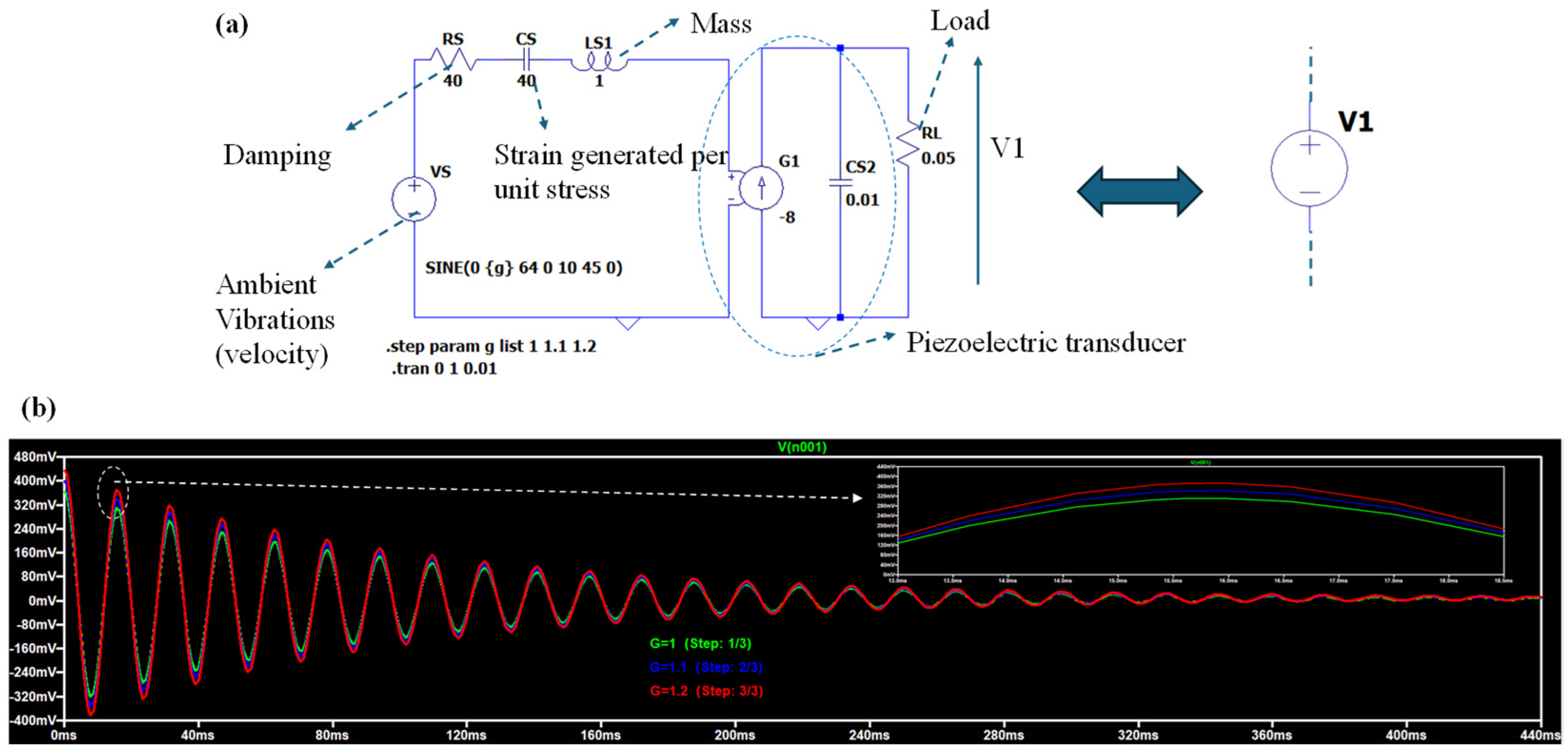
The whole physical effect integrates also the backward inverse piezoelectric effect: the generated electric field induces a mechanical strain (or a counter-acting force) modeling the shunt damping, decreasing the output power. This effect can be introduced by adding a resistance Rshunt in series with an inductance Lshunt [29,30] as illustrated in Figure A2.

Figure A2. (a) LTSpice modelling the equivalent voltage generator of Figure 3 by adding the inverse counter-acting force. (b) V1 signal estimated on the load resistance RL: the output voltage is further decreased by the backward inverse piezoelectric effect (V(n001) is the voltage calculated on the load resistance RL).

Figure A2. (a) LTSpice modelling the equivalent voltage generator of Figure 3 by adding the inverse counter-acting force. (b) V1 signal estimated on the load resistance RL: the output voltage is further decreased by the backward inverse piezoelectric effect (V(n001) is the voltage calculated on the load resistance RL).

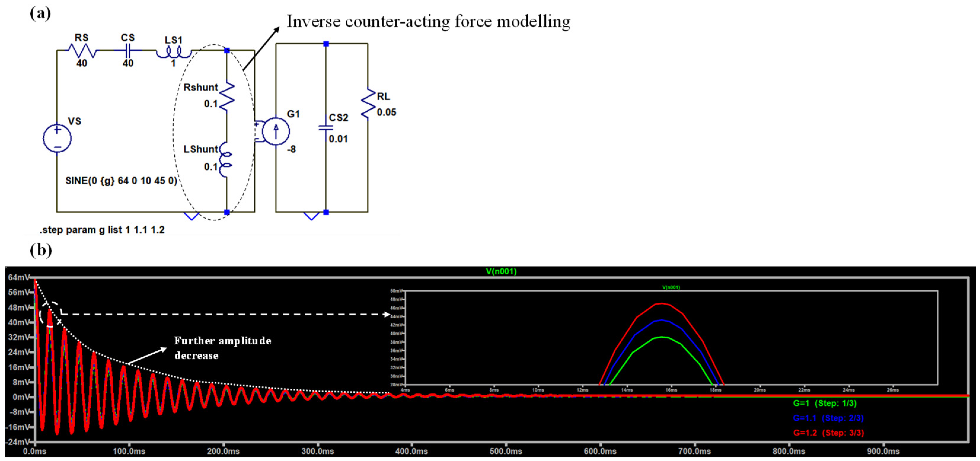
Figure A2 shows a further amplitude decrease by comparing the case of Figure 1. This decrease is defined by the dumping loss factor η. The output voltage calculated on the load assumes the form:

$$V_{out}\left(t\right)=A{e}^{-\eta {\omega }_{0}t}sen({\omega }_{0}t+\varphi )$$

(A1)

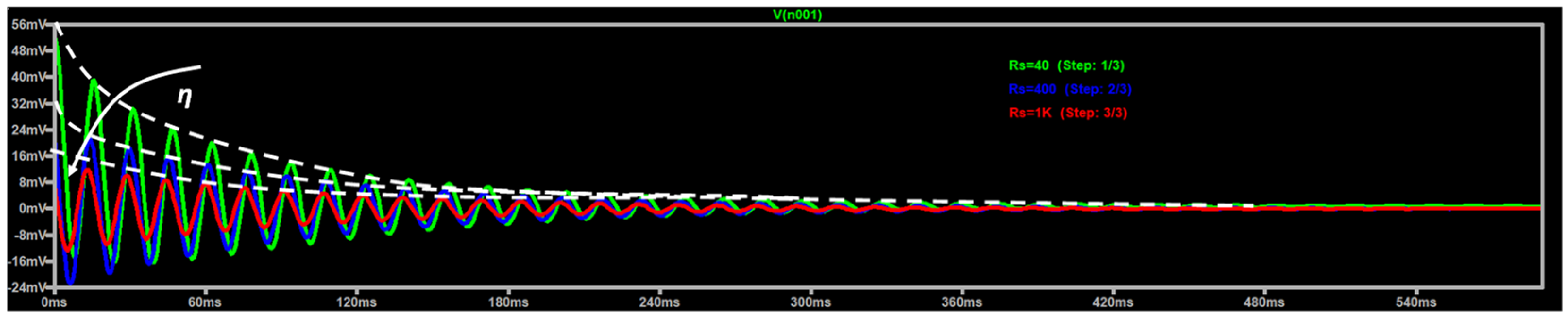
The loss effect of the loss is observed by the parametric analysis of Figure A3 by varying the damping resistance Rs of Figure A2a.

Figure A3. LTSpice parametric simulation of Figure A2a fixing the acceleration to 1 $\mathrm{g}$ (V(n001) is the voltage calculated on the load resistance RL). The white dashed lines indicate the damping trend.

Figure A3. LTSpice parametric simulation of Figure A2a fixing the acceleration to 1 $\mathrm{g}$ (V(n001) is the voltage calculated on the load resistance RL). The white dashed lines indicate the damping trend.

Appendix A.2. LTSpice Parametric Analysis of Load Variation

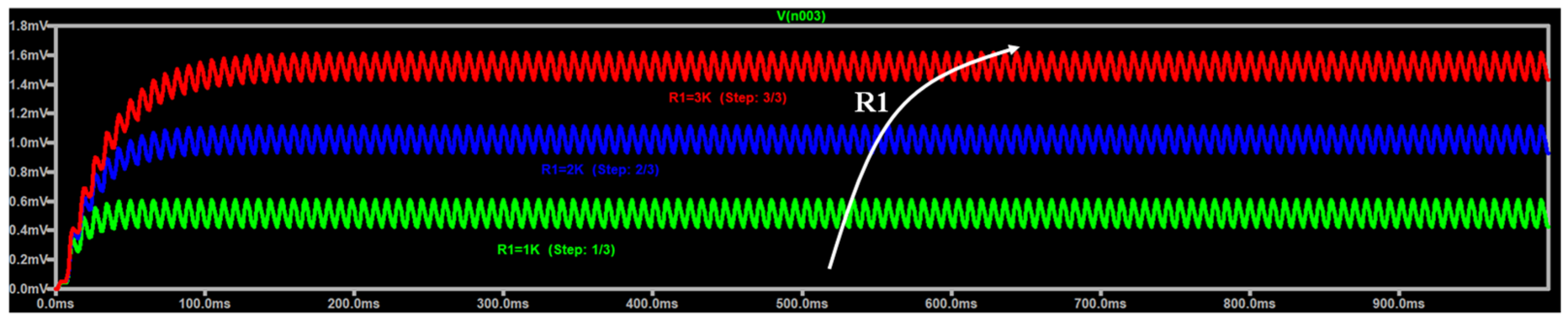
An example of voltage signal variation due to a change of the load R1 is illustrated in Figure A4: as expected the plot exhibits an increase of the output voltage by increasing the load resistance R1.

Figure A4. LTSpice parametric simulation varying the load R1 of Figure 3 and fixing a = 1 mm, Lp = Ls = 1.78 × 10⁻⁶ H and the acceleration to 1 $\mathrm{g}$ (V(n003) is the voltage calculated on the load resistance R1).

Figure A4. LTSpice parametric simulation varying the load R1 of Figure 3 and fixing a = 1 mm, Lp = Ls = 1.78 × 10⁻⁶ H and the acceleration to 1 $\mathrm{g}$ (V(n003) is the voltage calculated on the load resistance R1).

A metric to estimate the performance of the designed structure is the maximum amplitude which can be change with the variation of each parameter. An example is illustrated in Figure A5 by highlighting the differences at low frequencies (strong gap) and at the resonant frequencies (minor gap).

Figure A5. Spectra of the LTSpice parametric simulation varying the load R1 and fixing a = 1 mm, Lp = Ls = 1.78 × 10⁻⁶ H and the acceleration to 1 $\mathrm{g}$ (V(n003) is the voltage calculated on the load resistance RL). A slow amplitude variation is observed.

Figure A5. Spectra of the LTSpice parametric simulation varying the load R1 and fixing a = 1 mm, Lp = Ls = 1.78 × 10⁻⁶ H and the acceleration to 1 $\mathrm{g}$ (V(n003) is the voltage calculated on the load resistance RL). A slow amplitude variation is observed.

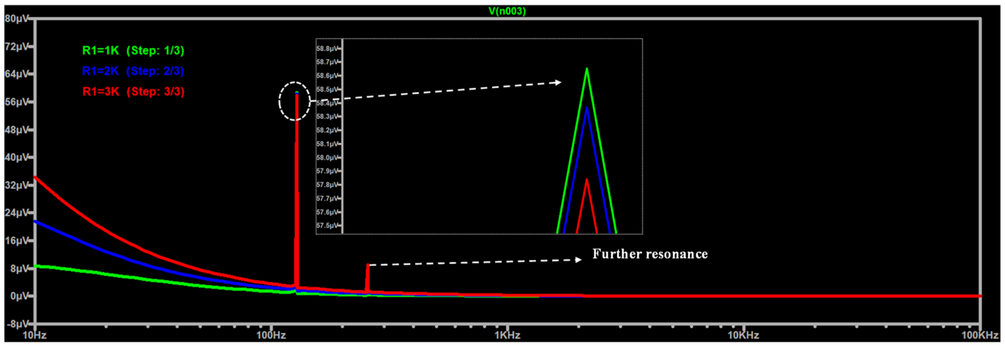
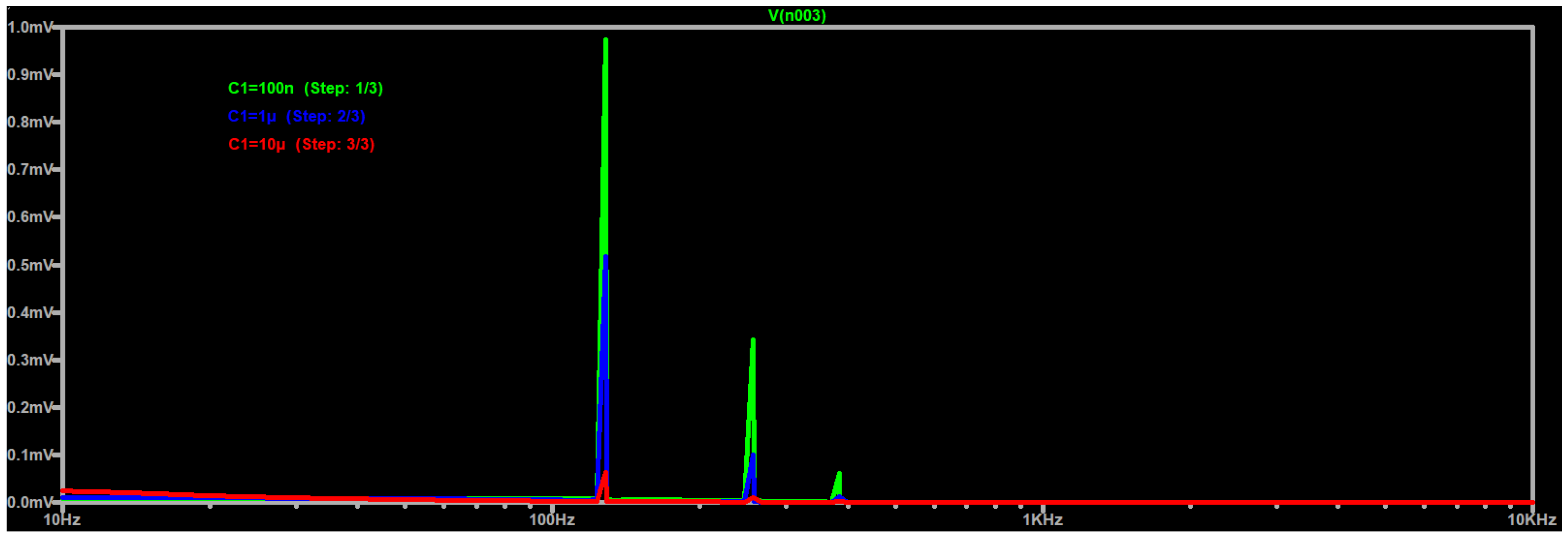
The variation of the load enables further resonances (see red peak of Figure A5). The whole circuit load is constituted by the parallel of R1 and C1 (see Figure 3). The peak amplitude variations and the presence of other resonance peaks is more visible by varying the capacitance C1 (see Figure A6).

Figure A6. Spectra of the LTSpice parametric simulation varying the capacitance C1 and fixing a = 1 mm, Lp = Ls = 1.78 × 10⁻⁶, R1 = 2000 Ω and the acceleration to 1 $\mathrm{g}$ (V(n003) is the voltage calculated on the load resistance RL). The simulation enhances the peak amplitude variations and the presence of other resonant peaks.

Figure A6. Spectra of the LTSpice parametric simulation varying the capacitance C1 and fixing a = 1 mm, Lp = Ls = 1.78 × 10⁻⁶, R1 = 2000 Ω and the acceleration to 1 $\mathrm{g}$ (V(n003) is the voltage calculated on the load resistance RL). The simulation enhances the peak amplitude variations and the presence of other resonant peaks.

Appendix A.3. LTSpice Parametric Analysis of Mechanical Efficiency

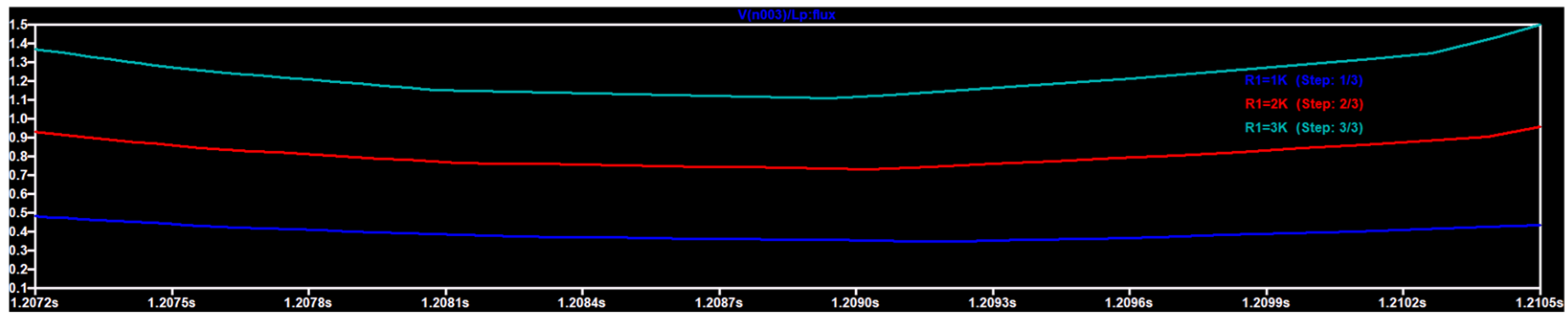
The mechanical efficiency can be estimated by the ratio Vout/VLp being VLp the voltage estimated between the nodes A and B of Figure 3. This ratio represents the fraction of the mechanical signal transduced into an electrical one and can change as a function of the geometric parameters downstream of the inductor Lp (values > 1 means amplification conditions). In Figure A7 is illustrated an example of estimation of the mechanical efficiency varying the load R1 of Figure 3.

Figure A7. LTSpice parametric simulation of the mechanical efficiency varying the load R1 of Figure 3 and fixing a = 1 mm, Lp = Ls = 1.78 × 10⁻⁶ H and the acceleration to 1 $\mathrm{g}$.

Figure A7. LTSpice parametric simulation of the mechanical efficiency varying the load R1 of Figure 3 and fixing a = 1 mm, Lp = Ls = 1.78 × 10⁻⁶ H and the acceleration to 1 $\mathrm{g}$.

Appendix A.4. Experimental Validation of the DT Model and Simulation Sensitivity

The FEM ΔV calculated in the proposed DT is compared with experimental results found in literature [31] finding a good matching (see Table A1), thus validating the applied methodology.

Table A1. Comparison between experimental results [31] and FEM ones (proposed DT) considering f₀ = 14.16 Hz as first natural frequency, a PZT5A length and thickness of 64 mm and 0.19 mm, respectively, and acceleration of 4 $\mathrm{g}$.

Piezoelectric ΔV [V] (Experimental [31])	Piezoelectric ΔV [V] (Proposed FEM)	Maximum Tip Displacement [mm] (Experimental [31])	Maximum Tip Displacement [mm] (Proposed FEM)
4.1	4.5	3.98	4.2

Table A1. Comparison between experimental results [31] and FEM ones (proposed DT) considering f₀ = 14.16 Hz as first natural frequency, a PZT5A length and thickness of 64 mm and 0.19 mm, respectively, and acceleration of 4 $\mathrm{g}$.

Piezoelectric ΔV [V] (Experimental [31])	Piezoelectric ΔV [V] (Proposed FEM)	Maximum Tip Displacement [mm] (Experimental [31])	Maximum Tip Displacement [mm] (Proposed FEM)
4.1	4.5	3.98	4.2

.

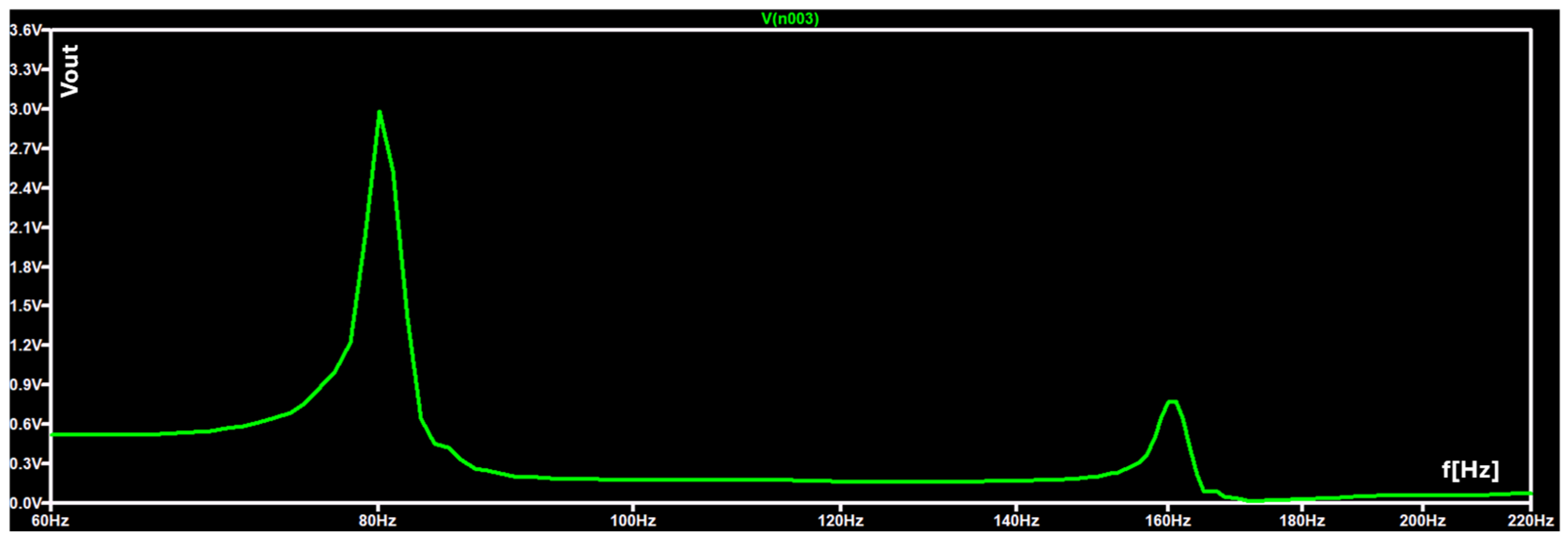
The implementation of DT model matching with experimental cases could be characterized by large dataset to process in cases to reply noisy conditions. In this direction could be adopted data-driven strategies able to decrease efficiently the training dataset [32]. One more comparison of the proposed DT with experimental results is illustrated in Figure A8 and Figure A9 proving a good matching of the frequency behavior: a resonance peak is found at 80 Hz both in FEM and in LTSpice simulation. The corresponding LTSpice circuit provides a further resonance at 160 Hz due to the whole circuit behavior of Figure 3.

Figure A8. Comparison between experimental output voltage [33] and DT FEM tip displacement versus frequency for a PZT5A having a length of 100 mm. The dashed arrows indicate the coordinate axis of the related plot.

Figure A8. Comparison between experimental output voltage [33] and DT FEM tip displacement versus frequency for a PZT5A having a length of 100 mm. The dashed arrows indicate the coordinate axis of the related plot.

Figure A9. LTspice: Output voltage versus the frequency corresponding to the structure of Figure A8 (Lp = Ls =1 × 10⁻³ H, R1 = 2000 Ω, C1 = 1 × 10⁻⁵ F).

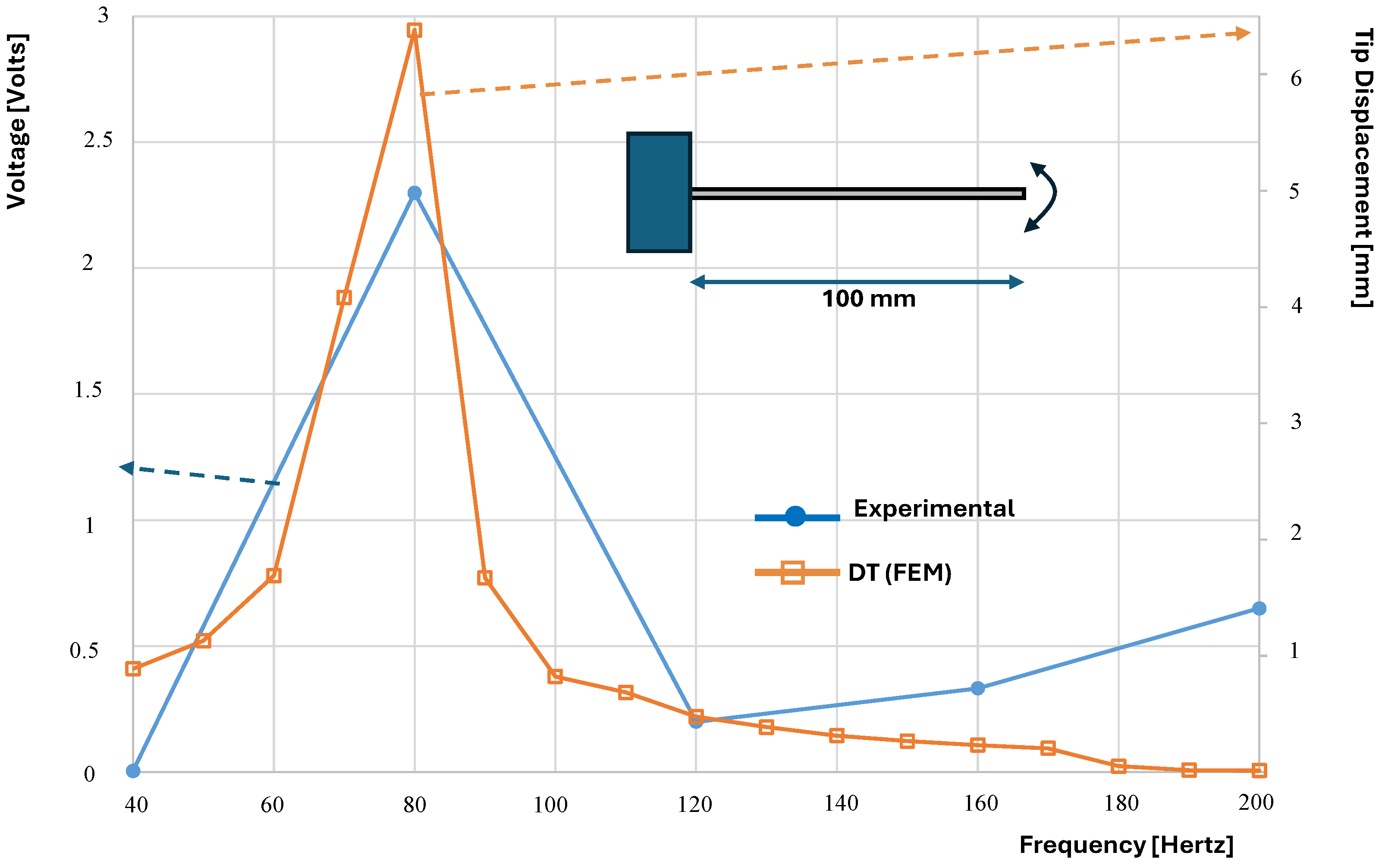
Figure A9. LTspice: Output voltage versus the frequency corresponding to the structure of Figure A8 (Lp = Ls =1 × 10⁻³ H, R1 = 2000 Ω, C1 = 1 × 10⁻⁵ F).

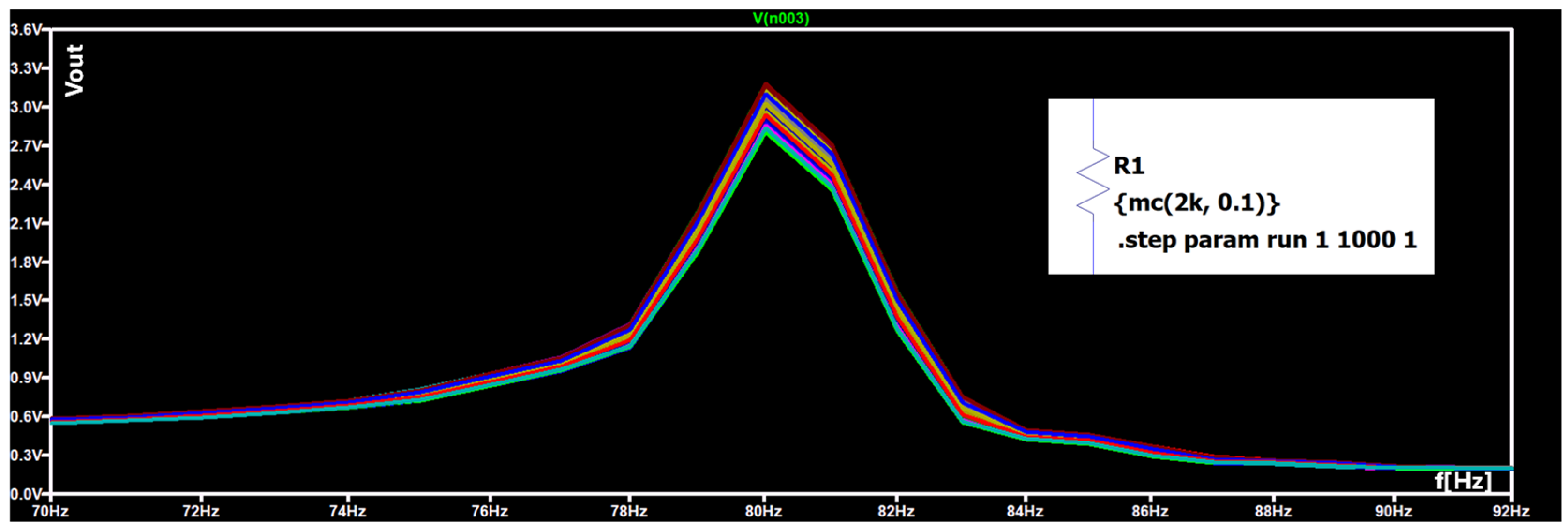
Experimental variability of signal amplitude error (voltage or power error) could be influenced by different aspects, such as electrical contacts losses or dealignments, temperature variations, vibration irregularities, or other forms of experimental setup misalignments. This can be modeled including the variability of circuit components and as a consequence the variability information of the measurements. Two tools frequently used for this purpose are the Monte Carlo method and the Worst Case Analysis (WCA) [27]. Specifically, the statistical approach of the Monte Carlo method is based on running a large number of simulations in which the values of each component are varied by evaluating the expected error of a given circuital parameter compared to its nominal value. By considering for example a load tolerance of the 10% for the circuit of Figure A9, a variability of the output voltage of ΔV = 0.4 Volt has been observed (see Figure A10).

Figure A10. LTspice: Monte Carlo simulations. Inset: modelling of the load variability (1000 simulations are performed in which the value of R1 is randomly varied, within the specified tolerance range of 2 kΩ ± 10%). A variability of ΔV = 0.4 Volt is observed at the resonance frequency of 80 Hertz. The colors refer to the different performed simulations.

Figure A10. LTspice: Monte Carlo simulations. Inset: modelling of the load variability (1000 simulations are performed in which the value of R1 is randomly varied, within the specified tolerance range of 2 kΩ ± 10%). A variability of ΔV = 0.4 Volt is observed at the resonance frequency of 80 Hertz. The colors refer to the different performed simulations.

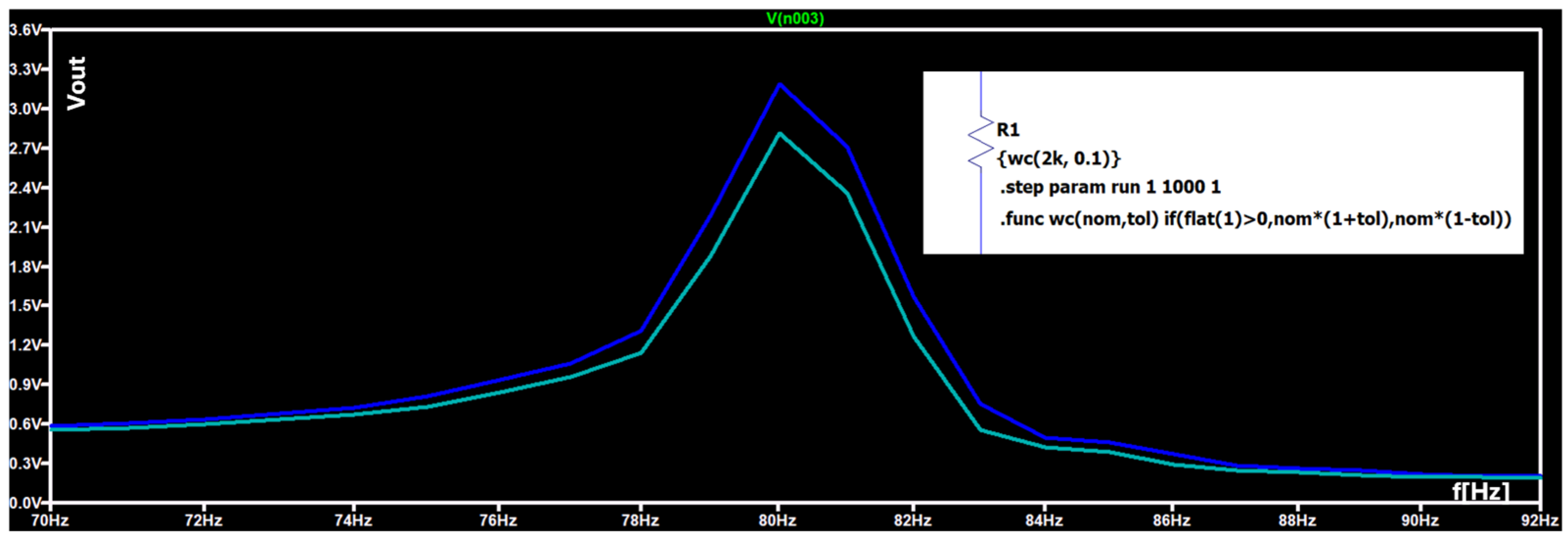
In addition, the WCA analysis is useful for predicting the maximum variation of a given parameter that could be obtained in the finished circuit, and modelling possible malfunctions correlated to the tolerances of the used components. In the proposed example, also for this case, a variability of the output voltage of about ΔV = 0.4 Volt has been found (see Figure A11).

Figure A11. LTspice: WCA analysis. Inset: modelling of the load variability within the specified tolerance range of 2 kΩ ± 10%. A variability of ΔV = 0.45 Volt is observed at the resonance frequency of 80 Hertz. The two colors indicate the variability range.

Figure A11. LTspice: WCA analysis. Inset: modelling of the load variability within the specified tolerance range of 2 kΩ ± 10%. A variability of ΔV = 0.45 Volt is observed at the resonance frequency of 80 Hertz. The two colors indicate the variability range.

References

- Massaro, A.; Cingolani, R. Parametric Analysis of Piezoelectric Resonances of AlN Layouts for Vibrating Energy Harvesting. J. Comput. Theor. Nanosci. 2011, 8, 2271–2278. [Google Scholar] [CrossRef] [Scilit]
- Massaro, A. Energy Harvesting Aspects of Irregular Vibrating Forces Acting on Piezoelectric Devices. In Innovative Materials and Systems for Energy Harvesting Applications; Mescia, L., Losito, O., Prudenzano, F., Eds.; IGI Global: New York, NY, USA, 2015. [Google Scholar] [CrossRef] [Scilit]
- Kiran, M.R.; Farrok, O.; Abdullah-Al-Mamun, M.; Islam, M.R.; Xu, W. Progress in Piezoelectric Material Based Oceanic Wave Energy Conversion Technology. IEEE Access 2020, 8, 146428–146449. [Google Scholar] [CrossRef] [Scilit]
- Gao, S.; Zhang, C.-Y.; Ao, H.-R.; Jiang, H.-Y. Performance of Beam-Type Piezoelectric Vibration Energy Harvester Based on ZnO Film Fabrication and Improved Energy Harvesting Circuit. Chin. Phys. B 2020, 29, 088401. [Google Scholar] [CrossRef] [Scilit]
- Yuan, M.; Cao, Z.; Luo, J. Characterization the Influences of Diodes to Piezoelectric Energy Harvester. Int. J. Smart Nano Mater. 2018, 9, 151–166. [Google Scholar] [CrossRef] [Scilit]
- Massaro, A.; De Guido, S.; Ingrosso, I.; Cingolani, R.; De Vittorio, M.; Cori, M.; Bertacchini, A.; Larcher, L.; Passaseo, A. Freestanding Piezoelectric Rings for High Efficiency Energy Harvesting at Low Frequency. Appl. Phys. Lett. 2011, 98, 053502. [Google Scholar] [CrossRef] [Scilit]
- Allaire, G.; Gfrerer, M.H. Autofreefem: Automatic Code Generation with FreeFEM and LaTex Output for Shape and Topology Optimization of Non-Linear Multi-Physics Problems. Struct. Multidiscipl. Optim. 2024, 67, 213. [Google Scholar] [CrossRef] [Scilit]
- Moszyński, M. Using FreeFEM Open Software for Modelling the Vibrations of Piezoelectric Devices. Vib. Phys. Syst. 2021, 32, 2021112-1–2021112-7. [Google Scholar] [CrossRef]
- Ma, G.; Zhou, P.; Zhang, H.; Qian, J.; Zhen, Y. Simulation of a Piezoelectric MEMS Accelerometer Using Finite Element Modeling with Freefem++. In Proceedings of the 21st International Conference on Electronic Packaging Technology (ICEPT), Guangzhou, China, 12–15 August 2020; IEEE: Piscataway, NJ, USA, 2020; pp. 1–5. [Google Scholar]
- Du, X.; Zhou, P.; Ren, H. Finite Element Modelling of a Piezoelectric MEMS Pressure Sensor Using FreeFem++. In Proceedings of the 24th International Conference on Electronic Packaging Technology (ICEPT), Shihezi, China, 8–11 August 2023; IEEE: Piscataway, NJ, USA, 2023; pp. 1–4. [Google Scholar]
- Herth, E.; Cavalliers, B.; Salhi, S.; Kardous, F.; Fall, D.; Rousseau, L.; Valbin, L.; Lardet-Vieudrin, F. Modeling and Characterization of Hybrid Thermo-Piezoelectric Cantilevers. J. Electron. Mater. 2025, 54, 3760–3772. [Google Scholar] [CrossRef] [Scilit]
- Brusa, E.; Carrera, A.; Delprete, C. Integrated Mechatronic Design of an Industrial Piezoelectric Vibration Energy Harvester. Mech. Adv. Mater. Struct. 2024, 31, 8966–8980. [Google Scholar] [CrossRef] [Scilit]
- Gonçalves, L.d.S.; Morais, M.C.; Medeiros, K.A.R.; Barbosa, C.R.H. Electrical Characterization and Modelling of Polyvinylidene Fluoride Thin Film for Application in Piezoelectric Energy Harvesting. ACTA IMEKO 2025, 14, 1–6. [Google Scholar] [CrossRef] [Scilit]
- Gao, A.; Li, B.; Han, M.; Liu, W.; Guan, W. Research on Self-Powered Sensors Based on Piezoelectric Energy Capture. In Mechanisms and Machine Science; Springer Nature: Switzerland, Cham, 2024; pp. 93–100. [Google Scholar]
- Edla, M.; Lim, Y.Y.; Deguchi, M.; Padilla, R.V. A Novel Discontinuous Mode Piezoelectric Energy Harvesting Circuit for Low-Voltage Applications. In Proceedings of the 31st Australasian Universities Power Engineering Conference (AUPEC), Perth, Australia, 26–30 September 2021; IEEE: Piscataway, NJ, USA, 2021; pp. 1–5. [Google Scholar]
- Sun, Y.-H.; Ye, X.-Q. Digital Twin of a Vibration Energy Harvesting System under Gaussian Noise Excitation. Chin. Phys. B 2025. [Google Scholar] [CrossRef] [Scilit]
- Ghosh, S.; Dan, S.; Tarafder, P. Machine Learning-Enabled Multiscale Modeling Platform for Damage Sensing Digital Twin in Piezoelectric Composite Structures. Sci. Rep. 2025, 15, 6631. [Google Scholar] [CrossRef] [Scilit]
- Park, J.G.; Kim, B.; Song, J.Y.; Ko, K.; Lee, H.K.; Choi, D.; Baek, S.; Park, S.M. Machine Learning-Driven Optimization of Locally Resonant Metamaterials for Simultaneous Vibration Control and Effective Triboelectric Sensing. Nano Energy 2025, 142, 111224. [Google Scholar] [CrossRef] [Scilit]
- Jing, Z.; Wang, Q.; Chen, Z.; Cao, T.; Zhang, K. Optimization of Energy Acquisition System in Smart Grid Based on Artificial Intelligence and Digital Twin Technology. Energy Inform. 2024, 7, 121. [Google Scholar] [CrossRef] [Scilit]
- Khan, H.; Khan, F.U. Vibration-to-Electricity Conversion: A Review of Electromagnetic, Electrostatic and Piezoelectric Energy Harvesters. SES 2025, 3, 1044–1087. [Google Scholar]
- Reddy, G.K.; Singh, P.; Ravi, K.C.; Anusha, B.; Gowri, C.; Vivek, R. Modeling and Analysis of MEMS Electrostatic Energy Harvesting System. J. Phys. Conf. Ser. 2024, 2837, 012104. [Google Scholar] [CrossRef] [Scilit]
- Kang, M.-G.; Jung, W.-S.; Kang, C.-Y.; Yoon, S.-J. Recent Progress on PZT Based Piezoelectric Energy Harvesting Technologies. Actuators 2016, 5, 5. [Google Scholar] [CrossRef] [Scilit]
- Piezoelectricity. Available online: https://modules.freefem.org/modules/piezoelectricity/ (accessed on 24 November 2025).
- Mountaciri, A.; Makroum, E.M.; Youssefi, M.A. Ltspice Simulation of Non Linear Technique SSHI Serial and SSHI Parallel of Piezoelectric Vibration Energy Harvesting. Int. J. Eng. Adv. Technol. 2021, 10, 87–94. [Google Scholar] [CrossRef] [Scilit]
- Massaro, A.; Lay-Ekuakille, A. Analysis of Magnetic Field Impact on Nanoparticles Used in Nanomedicine and a Measurement Approach. Measurement 2024, 226, 114167. [Google Scholar] [CrossRef] [Scilit]
- Massaro, A. Artificial Intelligence Enabling Denoising in Passive Electronic Filtering Circuits for Industry 5.0 Machines. Machines 2024, 12, 551. [Google Scholar] [CrossRef] [Scilit]
- Massaro, A. Electronic Artificial Intelligence–Digital Twin Model for Optimizing Electroencephalogram Signal Detection. Electronics 2025, 14, 1122. [Google Scholar] [CrossRef] [Scilit]
- Bonnin, M.; Song, K.; Traversa, F.L.; Bonani, F. A Circuit Theory Perspective on the Modeling and Analysis of Vibration Energy Harvesting Systems: A Review. Computation 2023, 11, 45. [Google Scholar] [CrossRef] [Scilit]
- Yan, B.; Wang, K.; Hu, Z.; Wu, C.; Zhang, X. Shunt Damping Vibration Control Technology: A Review. Appl. Sci. 2017, 7, 494. [Google Scholar] [CrossRef] [Scilit]
- Marakakis, K.; Tairidis, G.K.; Koutsianitis, P.; Stavroulakis, G.E. Shunt Piezoelectric Systems for Noise and Vibration Control: A Review. Front. Built Environ. 2019, 5, 64. [Google Scholar] [CrossRef] [Scilit]
- Khalatkar, A.; Gupta, V.K.; Agrawal, A. Analytical, FEA, and Experimental Comparisons of Piezoelectric Energy Harvesting Using Engine Vibrations. Smart Mater. Res. 2014, 2014, 741280. [Google Scholar] [CrossRef] [Scilit]
- Chen, H.; Niu, S.; Shao, Z.; Jian, L. Recognizing Multitype Misalignments in Wireless EV Chargers With Orientation-Sensitive Coils: A Data-Driven Strategy Using Improved ResNet. IEEE Trans. Ind. Inform. 2024, 20, 280–290. [Google Scholar] [CrossRef] [Scilit]
- Kshirsagar, S.R.; Ghatage, V.R.; Kolgiri, S.G. PZT Material as an Energy Harvester. In Proceedings of the National Conference on Technological Developments in Civil and Mechanical Engineering (NCTDCME-18), Indapur, India, 15–16 March 2018. [Google Scholar]
Disclaimer/Publisher’s Note: The statements, opinions and data contained in all publications are solely those of the individual author(s) and contributor(s) and not of MDPI and/or the editor(s). MDPI and/or the editor(s) disclaim responsibility for any injury to people or property resulting from any ideas, methods, instructions or products referred to in the content. |
© 2026 by the authors. Licensee MDPI, Basel, Switzerland. This article is an open access article distributed under the terms and conditions of the Creative Commons Attribution (CC BY) license.