


Abstract
This paper assesses the Wind Power Penetration Limit (WPPL) of the Colombian Caribbean Power System through a scenario-based parametric sensitivity analysis. The study is conducted on a newly developed open-source 36-bus testbed implemented in Pandapower, representing the 500 kV and 230 kV interconnected network and its five operational subareas: Córdoba-Sucre, Bolívar, Atlántico, Cerromatoso, and Guajira-Cesar-Magdalena. The proposed framework determines the maximum wind power integration capacity at each substation while quantifying the sensitivity of key operating variables, including frequency, voltage magnitude, voltage angle, and loadability. The assessment combines frequency critical times (), voltage-reactive power sensitivity (), voltage security margins, loadability limits, and N-k contingency analysis (). Wind generation levels are progressively increased from 1 MW to 2400 MW, and the frequency stability evaluation considers doubly fed induction generator (DFIG), full-converter, full-converter with synthetic inertia, and vertical-axis wind turbine technologies. Within the adopted reduced-order parameterization, the DFIG-labeled configuration produces the longest threshold-event times. This ordering follows from the prescribed effective-inertia coefficients and does not establish a universal frequency-stability ranking of wind-turbine technologies. From a security perspective, the Córdoba-Sucre subarea exhibits the highest resilience under contingencies, whereas the Atlántico subarea presents the largest wind integration capability. In contrast, the Bolívar subarea shows the greatest susceptibility to instability, while Cartagena and Barranquilla emerge as the most congestion-prone locations. Overall, the proposed framework provides a reproducible methodology for identifying substation-level WPPL values and supporting large-scale wind integration planning in interconnected power systems.
1. Introduction
Across Latin America [1], and particularly within the current context of the Colombian energy sector [2], the integration of non-conventional renewable energy sources into power systems has gained significant relevance. This is mainly due to the identification of significant renewable energy potential, and regulatory frameworks that encourage the rational and efficient use of energy [3]. To this end, public and private entities from the academic community and the energy sector are actively developing studies and analytical tools that enable the precise quantification of the integration potential and optimal locations of these resources in real-world energy markets. These non-conventional energy sources are characterized primarily by their low or near-zero emissions and the variability and intermittency of their power generation; in the case of solar, wind, or tidal energy, this volatility is significant and it is reflected in fluctuations in power output due to variations in resource availability. Such properties make technical constraints particularly important when assessing, evaluating, or planning the renewable energy integration.
To account for these aspects, potential assessment and planning studies for the integration of renewable generation into the grid consider multiple factors such as meteorological conditions, geographic location, and environmental, ecological, social, and accessibility constraints, among others [4]. From a technical perspective, the most common criteria are system sizing and proximity to the electrical grid, particularly to transmission lines. Although these restrictions provide a general overview of the potential integration of such sources within the energy system, a more realistic approach must consider whether locations with renewable energy potential can be effectively connected to the grid while delivering their rated capacity. In practice, the realizable generation is constrained by the network absorption capacity at the bus where the new source is integrated. This makes the hosting capacity of each bus a primary constraint for renewable energy integration.
The Colombian Caribbean Power Network, shown in Figure 1, is an interconnected high-voltage system spanning seven departments and operating at 500, 230, and 220 kV voltage levels. Large-scale renewable generation projects are represented by graduated markers indicating their installed capacity, while transmission lines are displayed according to their voltage level. To assess the feasibility of integrating new renewable power plants, electrical infrastructure, operating conditions, and grid absorption capacity are critical factors, as they directly affect project feasibility and associated costs. Quantifying the hosting capacity at each grid connection point is therefore essential to identify locations with the greatest wind potential, evaluate connection alternatives, and estimate the costs associated with bay expansions, transmission line extensions, new substations, and other network reinforcements. This requires defining a simple yet comprehensive indicator capable of characterizing each connection point while accounting for system behavior under new generation integration scenarios. This approach enables the assessment of hosting capacity, particularly for wind power integration, whose variability and converter-based interfacing may significantly affect system stability and frequency regulation.
Figure 1.
Colombian Caribbean power system and geographic location of existing generation projects. Transmission lines are color-coded according to their capacity levels, while generation projects are represented by graduated markers whose color scale ranges from gray (lower installed capacity) to fuchsia (higher installed capacity). Spanish geographic labels inherited from the source basemap denote place names and protected areas; for example, “Golfo de Darién” means “Gulf of Darién”.
In this work, the maximum wind power penetration limit, expressed in MW, is determined using a novel regional model and an integrated assessment of bus stability and system security. This definition differs from those commonly reported in the literature. The proposed approach captures the electric constraints associated with each bus in a simple manner, making it suitable for wind energy potential assessment studies. Since the objective is to estimate this limit for all potential connection points in the system, a testbed based on the Colombian power system is developed to perform power-flow analyses and implement a methodology that integrates stability and security margins to constrain wind power penetration. This framework also provides an opportunity to evaluate transmission network investments and synthetic inertia requirements associated with wind energy integration [5]. Assessing system stability under increasing wind power integration is essential for understanding the flexibility of the network to accommodate new generation and the amount of wind power that can be reliably committed to the electricity market under future development scenarios.
Regarding wind power penetration limits, the literature reports a variety of WPPL definitions. In [6], a study of large-scale wind integration into the Turkish power system is reported, emphasizing the evaluation of P–V and Q–V curves to assess static voltage stability limits under generation outage scenarios. The results provide a system-wide stability margin expressed in MW. A similar approach is adopted in this work; however, it is applied to each network connection point through the proposed WPPL indicator. Another related study is presented in [7], which investigates the effects of wind energy integration on voltage stability using a Double Fed Induction Generator (DFIG) connected to the Ethiopian 230 kV transmission network. The study evaluates different wind speed scenarios for a 120 MW wind farm connected to a two-bus testbed. P–V curves are obtained through continuation power flow analysis at the two buses of the test system. The wind farm is integrated into a modified IEEE 57-bus system comprising four generators and 42 loads. To the best of the authors’ knowledge, no similar study has been reported for the Colombian power system.
The literature reports several studies addressing WPPL estimation and the role of stability analysis in wind energy integration. For example, Ref. [8] presents a computational, data-driven methodology for evaluating renewable energy integration limits from a frequency stability perspective, providing insights for system planners, operators, and policymakers regarding the impacts and benefits of renewable energy adoption. The study focuses on system operation and employs a simplified four-area model of the Australian power system with ZIP load representations, analyzing 100% renewable and prosumer scenarios for 2040. Similarly, Ref. [9] investigates WPPL from a frequency stability perspective. Likewise, Ref. [10] estimates the WPPL using a frequency security index for the entire system, defines WPPL as the ratio between total wind generation and total synchronous generation capacity, and applying a critical time analysis framework. In [11], the authors investigate the wind power penetration limit under transient rotor-angle stability constraints using an optimal power flow formulation applied to the IEEE 14-bus system (259 MW total load and five generators). The framework incorporates contingency analysis and determines penetration levels relative to system load. The study establishes a single penetration limit for the entire network using a fourth-order dynamic synchronous generator model and Weibull-distributed wind conditions. The analysis focused on operational limits rather than long-term planning applications. Existing studies generally determine a single WPPL value for the entire system, whereas the proposed methodology estimates penetration limits individually for each network connection point, making it more suitable for planning and renewable resource assessment studies.
Figure 2 shows the spatial distribution of wind-resource potential and the transmission infrastructure considered in the study area.
Figure 2.
Colombian Caribbean transmission system and wind-resource distribution. The map presents the 220/230 kV and 500 kV transmission lines and substations within the study area. Wind-resource potential is represented by a graduated color scale, where pink, orange, and golden regions denote the highest resource availability. The concentration of high-potential areas in the northern Caribbean region motivates the assessment of grid hosting capacity for future renewable energy integration.
In [12], a modal eigenvalue analysis method is applied to evaluate the WPPL, by assessing voltage stability through analytical sensitivity models relating bus voltage to reactive power injections. The overall WPPL is expressed as a function of the relationship between wind generation and load demand. Similarly, Ref. [13] presents a WPPL assessment based on a Thevenin-equivalent representation of the power system and investigates penetration limits under different loading conditions. These studies introduce different approaches for estimating the WPPL; however, a major limitation is that they do not explicitly quantify hosting capacity of individual buses. Furthermore, stability and security are treated independently, and even when the methods are applied to small test systems, the resulting metrics do not provide a direct quantification of hosting capacity at each connection point. Therefore, the methods available in the literature are not directly applicable to the problem addressed in this work. Finally, Ref. [14] wind power ramp-rate limitations and the potential reduction of energy curtailment through the integration of battery energy storage systems. This work focuses on short-term operational behavior and can therefore be classified as an intra-day analysis.
Meanwhile, the literature on the Colombian power system and the Colombian Caribbean transmission network includes several studies addressing renewable energy integration, system flexibility, and network modeling. For example, Ref. [15] presents a study on power system flexibility, analyzing the impact of renewable energy integration on the operation of existing generation resources. The study applies load-ramping scenarios and evaluates renewable energy integration limits while maintaining secure and stable system operation. The methodology is market-oriented and uses historical demand data to project future scenarios, considering a generation mix composed of hydroelectric, thermal, wind, biomass, and solar resources. The study subsequently analyzes renewable integration ramps and evaluates whether conventional generation is capable of compensating for renewable generation variability under future operating conditions. Although the study provides a valuable assessment of flexibility in the Colombian electricity market, it does not include stability analyses of the proposed generation capacities using a transmission network test system. Furthermore, the study does not quantify hosting capacity at individual buses or evaluate security and stability constraints at specific network connection points, which are key aspects of the methodology proposed in this work.
The study subsequently analyzes renewable integration ramping scenarios and evaluates whether conventional generation resources are capable of compensating for renewable generation variability under future operating conditions. Although the study provides a valuable assessment of flexibility in the Colombian electricity market, it does not include stability analyses of the proposed generation capacities using a transmission network test system.
A simplified test system of the Colombian power system is presented in [16] to analyze and compare different controller strategies for wind power integration. The system consists of a fixed configuration comprising five areas, 20 buses, 13 synchronous generators, and 16 converter-based generation units. The corresponding system data are reported in [17]. Similarly, Ref. [18] presents two test systems for distributed power system simulation: a 33-bus system representing the metropolitan area of Medellín and a 27-bus system located in Capurganá, Chocó. These test systems were developed to study optimal market dispatch considering solar photovoltaic (PV) generation. Distribution networks, which typically operate at voltages levels below 100 kV, are suitable for studying distributed generation. However, the present work focuses on wind power penetration in high-voltage transmission networks.
Building upon these studies, this work develops a simulation-based methodology for estimating the WPPL at each network connection point incorporating stability and security indicators of the interconnected power system. The proposed analysis combines voltage stability, rotor angle, frequency, and contingency criteria to determine the wind power hosting capacity of each connection point. Unlike previous studies, the objective is to characterize the capability of the system to accommodate new wind generation rather than to maximize penetration levels or evaluate wind generation as a percentage of system load. Furthermore, the methodology differentiates operational subareas and connection points, enabling its application to generation and transmission expansion planning as well as project prioritization based on technical integration criteria. In addition, the analysis incorporates simplified electromechanical dynamics through the swing equations, which are used to represent virtual synchronous generators at different connection points and to evaluate system behavior under varying inertia conditions associated with different wind turbine technologies.
The methodology for calculating wind power penetration limits is based on voltage stability margins obtained from P-V Curves and Q-V curves, voltage angle differences, and critical clearing times evaluated at different buses under increasing wind power integration scenarios. In addition, these margins are evaluated under N-1 and N-2 contingency conditions, while transmission line loadability is assessed across different operating scenarios. The indicators are not combined through numerical weights. The candidate penetration limits are evaluated through a hierarchical decision rule in which a binding criterion cannot be compensated by a favorable value of another indicator. The resulting WPPL and the ordinal security ranking are reported separately. The main advantage of the proposed WPPL indicator is that it is defined with respect to potential generation capacity rather than system demand. Moreover, it is a spatially distributed indicator that can be calculated for individual geographic locations and connection points within the network, rather than as a single aggregated value for the entire system or a specific region. Furthermore, unlike existing approaches reported in the literature, the proposed indicator integrates multiple technical criteria, providing a more comprehensive assessment of system behavior and stability under increasing wind power integration. The proposed methodology and the resulting analyses provide a deeper understanding of system stability across multiple operational dimensions, enabling a technical characterization of each location within the Colombian Caribbean transmission network.
The remainder of the paper is organized as follows. Section 2 presents the system model and the proposed methodological framework, including the analytical procedures applied to each evaluation criterion. Section 3 presents the results, which are divided into three parts: (1) analysis of voltage stability through P–V and Q–V curves, together with voltage angle differences across transmission lines, to establish voltage stability criteria; (2) contingency analysis (N-1 and N-2) and critical clearing time assessments to evaluate transmission line loadability under different wind power penetration levels; and (3) characterization of each network node and determination of its wind power hosting capacity through the proposed WPPL indicator. Section 4 interprets the results by examining system behavior from stability and security perspectives and outlining future research directions involving wind generation profiles and distributed generation resources. Finally, Section 5 summarizes the main conclusions of this work.
2. Methods
The Wind Power Penetration Limit (WPPL) represents the maximum wind generation capacity that can be accommodated at each bus of the power system. The proposed methodology aims to estimate the wind power penetration limit (MW) at every candidate connection point within the Colombian Caribbean Network by integrating voltage stability, angle stability, frequency response, and / contingency criteria. As part of this work, a simplified model of the Colombian Caribbean power system is developed, providing a new test system that has not been previously reported in the literature. The methodological framework consists of four stages, as illustrated in Figure 3. Two of these stages are jointly implemented within a single analytical workflow because they rely on the same set of simulations and indicators. The framework includes system modeling (Section 2.1), data generation and indicator assessment (Section 2.2), and WPPL calculation and ranking (Section 2.3).
Figure 3.
Flowchart of the proposed assessment methodology for determining Wind Power Penetration Limits (WPPL). The framework comprises four stages: grid modeling in pandapower using UPME and XM data; virtual wind generation scenario generation; stability indicators assessment (, , and curves, frequency stability, and / contingencies); and bus ranking to assign the WPPL based on the most limiting stability criterion.
In the first stage, information related to all components of the electrical system is collected and organized into a database from which a system model is developed in Python 3.10.19 using Pandapower. The data employed for model construction are obtained from official records of the Colombian National Interconnected System and are publicly available through the Ministry of Mines and Energy, the Mining and Energy Planning Unit (UPME) [19], and XM’s PARATEC platform [20]. Leveraging Pandapower’s capability to perform alternating-current power flow simulations, a set of analysis routines is developed to implement the proposed methodology, which is based on stability assessment and contingency analysis. The implementation details of the developed routines are provided in Appendix C.
The second and third stages focus on the development of analytical tools for assessing voltage, angle, frequency, and transmission line loadability throughout the system. In addition, and contingency scenarios are generated to evaluate system performance under different wind power penetration levels. Stability and security assessments are performed by analyzing the response of the network to the integration of new wind generation. The corresponding analysis routines are implemented in Python using the Pandapower library (see Appendix C). Following the system analysis, a set of indicators is calculated for each bus, including the Voltage-Based Power Penetration Limit (VBPPL), Reactive Power-Based Power Penetration Limit (QBPPL), Frequency-Based Power Penetration Limit (FBPPL), as well as the operating state of the system and associated indicators under and contingency conditions.
Finally, in the fourth stage, the database of calculated variables and indicators is used to rank the network buses according to their suitability for the integration of new wind generation, ranging from the most secure and stable locations to those operating close to their base-case limits. Based on this ranking, WPPL values are determined for each bus, thereby characterizing the capability of each substation to accommodate additional wind generation and quantifying the amount of wind power that can be integrated. The resulting assessment provides a technical characterization of the connection points within the network and supports the identification of the most suitable locations for future wind energy development. The following sections describe each stage of the methodology in detail.
2.1. System Modelling
In this work, the Pandapower toolbox is used to develop the Colombian power system testbed. Pandapower is an open-source Python-based framework originally designed for the analysis of balanced power systems and can be readily integrated with other open-source libraries without licensing restrictions [21]. The implemented models and algorithms have been validated through performance comparisons with commercial power system analysis software. Pandapower provides a flexible and user-friendly environment for conducting a wide range of power system studies in both transmission and distribution networks. The framework employs an Element-Based Model (EBM) to represent electrical networks [21], facilitating the conversion and integration of data from commercial software tools. By decoupling the element representation from the underlying electrical model, Pandapower enables the implementation of different modeling approaches tailored to specific analysis requirements. Furthermore, the framework adopts a tabular data structure in which each network element is represented by dedicated tables containing its parameters and simulation results. This architecture supports the storage of heterogeneous data types, allowing the integration of metadata, operating states, and model parameters within a unified environment.
Pandapower is built on the Python pandas library, allowing users to leverage pandas functionalities for network management, data processing, and analysis. All network information is stored in a Python dictionary named net, which contains element and result tables for every system component. The framework provides models for buses, loads, static generators, voltage-controlled generators, external grids, shunts, lines, two-winding transformers, three-winding transformers, switches, DC transmission lines, impedances, and Ward equivalents. Figure 4 illustrates the single-line diagram of the interconnected power system in the Colombian Caribbean region, including the Bolívar, Atlántico, Córdoba-Sucre, and Guajira-Cesar-Magdalena (GCM) operational subareas. Each subarea is analyzed both individually and as part of the complete network to identify its static and dynamic behavior and to evaluate the impact of integrating new generation sources on system performance. The objective of this analysis is to assess the wind energy integration capacity of the network while considering the technical constraints of the Colombian National Interconnected System. A summary of the system data is provided in Appendix A.
Figure 4.
Topological single-line representation of the Colombian Caribbean power grid illustrating voltage levels, busbar connections, and geographical clustering across five operational sub-areas (Bolívar, Atlántico, GCM, Córdoba–Sucre, and Cerromatoso). The symbol G denotes a generating unit, paired circles denote transformers, downward arrows denote loads, thick bars denote busbars, and colored outlines identify the operational subareas.
Using the Pandapower toolbox, the interconnected system is reconstructed by operational subareas, including the transmission-line interconnections between them. Each subnetwork is modeled using specific Pandapower functions and network elements. As an example, the following code illustrates the implementation of the Bolívar subarea, which forms part of the Colombian Caribbean interconnected power system. Detailed information on the model development process is provided in Appendix C, including Algorithms A1–A3.
The data used to develop the interconnected system model are obtained from the Mining and Energy Planning Unit (UPME) through the Colombian Electrical Infrastructure Viewer available on the national open-data portal [19]. These data are exported to databases and subsequently used for model development, simulation, and visualization in ArcGIS Online (Esri, web version accessed in July 2026), where georeferencing and complementary information management are also performed. Additional network data are obtained from PARATEC, including the electrical parameters of transmission lines, substations, generating units, and transformers.
import pandapower as pp

def crear_red_bolivar():
    net = pp.create_empty_network(f_hz=60, sn_mva=100)
    factor = 0.78

# Buses 500 kV

    bus_bolivar500 = pp.create_bus(net, vn_kv=500, name="Bolivar 500kV")
    #bus_elcopey500 = pp.create_bus(net, vn_kv=500, name="El Copey 500kV")
    #bus_sabanalarga500 = pp.create_bus(net, vn_kv=500, name="Sabanalarga 500kV")

# Buses 220 kV

    bus_bolivar230 = pp.create_bus(net, vn_kv=230, name="Bolivar 230kV")
    bus_termocandelaria220 = pp.create_bus(net, vn_kv=220, ...
    ... name="Termocandelaria 220kV")
    bus_ternera220 = pp.create_bus(net, vn_kv=220, name="Ternera 220kV")
    bus_elbosque220 = pp.create_bus(net, vn_kv=220, name="El Bosque 220kV")
    bus_cartagena220 = pp.create_bus(net, vn_kv=220, name="Cartagena 220kV")
    #bus_sabanalarga230=pp.create_bus(net, vn_kv=230, name="Sabanalarga 230kV")

# 500 kV lines

    #pp.create_line_from_parameters(net, bus_bolivar500, bus_elcopey500,...
    ...length_km=166.68, r_ohm_per_km=0.0237, x_ohm_per_km=0.3342, c_nf_per_km=0,
    ...g_us_per_km=4.9138, max_i_ka=2.476, type= "ol",
    ...name="Bolivar-El Copey 1 500kV")
    # pp.create_line_from_parameters(net, bus_bolivar500, bus_sabanalarga500,
    ...length_km=66.556, r_ohm_per_km=0.0239, x_ohm_per_km=0.3183, c_nf_per_km=0,
    ...g_us_per_km=5.1626, max_i_ka=3.120, type= "ol",
    ...name="Bolivar-Sabanalarga 1 500kV")
    pp.create_line_from_parameters(net, bus_cartagena220, bus_termocandelaria220,
    ...length_km=2.88, r_ohm_per_km=0.0892, x_ohm_per_km=0.4973, c_nf_per_km=0,
    ...g_us_per_km=3.3444, max_i_ka=0.813, type= "ol",
    ...name="Cartagena-Termocandelaria 1 230kV")
    pp.create_line_from_parameters(net, bus_cartagena220, bus_termocandelaria220,
    ...length_km=2.88, r_ohm_per_km=0.0892, x_ohm_per_km=0.4973, c_nf_per_km=0,
    g_us_per_km=3.3444, max_i_ka=0.813, type= "ol",
    ...name="Cartagena-Termocandelaria 2 230kV")
    pp.create_line_from_parameters(net, bus_termocandelaria220, bus_ternera220,
    ...length_km=3.12, r_ohm_per_km=0.0896, x_ohm_per_km=0.4955, c_nf_per_km=0,
    ...g_us_per_km=3.3608, max_i_ka=0.813, type= "ol",
    ...name="Termocandelaria-Ternera 1 230kV")
    pp.create_line_from_parameters(net, bus_termocandelaria220, bus_ternera220,
    ...length_km=3.12, r_ohm_per_km=0.0896, x_ohm_per_km=0.4955, c_nf_per_km=0,
    ...g_us_per_km=3.3608, max_i_ka=0.813, type= "ol",
    ...name="Termocandelaria-Ternera 1 230kV")
    pp.create_line_from_parameters(net, bus_elbosque220, bus_ternera220,
    ...length_km=25.69, r_ohm_per_km=0.0602, x_ohm_per_km=0.452, c_nf_per_km=0,
    g_us_per_km=13.5127, max_i_ka=0.830, type= "ol",
    ...name="El Bosque-Ternera 1 230kV")
    #pp.create_line_from_parameters(net, bus_sabanalarga230, bus_ternera230,
    ... length_km=80.18, r_ohm_per_km=0.0893, x_ohm_per_km=0.496, c_nf_per_km=0,
    ...g_us_per_km=3.3541, max_i_ka=0.813, type= "ol",
    ...name="Sabanalarga-Ternera 1 230kV")


# 220 kV lines
    pp.create_line_from_parameters(net, bus_bolivar230, bus_elbosque220,
    ...length_km=17.29, r_ohm_per_km=0.049, x_ohm_per_km=0.384, c_nf_per_km=0,
    ...g_us_per_km=18.445, max_i_ka=0.800, type= "ol",
    ...name="Bolivar-El Bosque 1 230kV")
    pp.create_line_from_parameters(net, bus_bolivar230, bus_cartagena220,
    ...length_km=18.3, r_ohm_per_km=0.063, x_ohm_per_km=0.491, c_nf_per_km=0,
    ...g_us_per_km=3.371, max_i_ka=0.929, type= "ol",
    ...name="Bolivar-Cartagena 1 230kV")
    pp.create_line_from_parameters(net, bus_bolivar230, bus_cartagena220,
    ...length_km=18.3, r_ohm_per_km=0.063, x_ohm_per_km=0.491, c_nf_per_km=0,
    ...g_us_per_km=3.371, max_i_ka=0.929, type= "ol",
    ...name="Bolivar-Cartagena 2 230kV")

# Transformers
    pp.create_transformer_from_parameters(net, bus_bolivar500, bus_bolivar230,
    ...sn_mva=900, vn_hv_kv=500, vn_lv_kv=230, vk_percent=11.71, vkr_percent=0.5,
    ... i0_percent=0.1, pfe_kw=150, shift_degree=0, name="Trafo Bolivar 900MVA")

# Generators
    pp.create_gen(net, bus_termocandelaria220, p_mw=659.3,...
    ...vm_pu=1.0, name="Termocandelaria")
    pp.create_gen(net, bus_cartagena220, p_mw=222.3, ...
    ...vm_pu=1.0, name="Cartagena")

# Loads
    pp.create_load(net, bus_cartagena220, p_mw=factor*237.5, ...
    ... q_mvar=factor*12.5, name="Carga Cartagena 230kV")
    pp.create_load(net, bus_ternera220, p_mw=factor*399, ...
    ...q_mvar=factor*21, name="Carga Ternera 230kV")
    pp.create_load(net, bus_elbosque220, p_mw=factor*427.5, ...
   ...q_mvar=factor*22.5, name="Carga El Bosque 230kV")
    pp.create_load(net, bus_bolivar230, p_mw=factor*190, ...
    ...q_mvar=factor*10, name="Carga Bolivar 230kV")
    pp.create_load(net, bus_termocandelaria220, p_mw=factor*237.5,...
    ...q_mvar=factor*12.5, name="Carga Termocandelaria 230kV")

# Slack temporal
   # pp.create_ext_grid(net, bus_bolivar500,...
   ...vm_pu=1.0, name="Slack Bolívar")

    return net# -*- coding: utf-8 -*-
The implementation begins by creating a net object operating at 60 Hz, representing the Colombian National Interconnected System, and adopting a per-unit base power of 100 MVA. The 500 kV buses are first modeled, followed by the reconstruction of the 220 kV and 230 kV buses, with an identifying label assigned to each network element. Subsequently, the 500 kV transmission network is incorporated into the model. The parameters required for each transmission line include the sending and receiving buses, line length (km), series resistance and reactance (Ω/km), shunt capacitance (nF/km), maximum current rating (kA), and an associated identifier tag.
Transformers connecting the 500 kV and 230 kV voltage levels are also incorporated into the model. The parameters required for each transformer include the sending and receiving bus indices, rated power (MVA), nominal voltages on the high- and low-voltage sides, short-circuit voltage, short-circuit resistance, no-load losses, no-load current, phase shift angle, and transformer identifier.
Generating units are represented in the net object using parameters such as the bus index, active power output, voltage setpoint, and unit name. The framework allows the independent connection of an arbitrary number of generators at any network location. This capability is extensively used throughout the proposed methodology, where additional generation capacity is simulated by connecting new generation units with predefined power ratings to the buses specified in each study scenario.
For load modeling, each demand point is represented in the net object by its corresponding bus index, active power demand (MW), reactive power demand (MVAr), and identifier. Active and reactive power values are assigned according to a medium-to-high demand scenario reported by UPME. To distribute the load across the transmission network, the methodology first identifies the connection points between the 230 kV and 115 kV networks, which correspond to 230/115 kV transformers. Since the focus of this study is the high-voltage transmission system, the 115 kV network and all lower-voltage elements are excluded from the model. At each interface point, the corresponding transformer is replaced by an equivalent load whose maximum value is based on the transformer’s nominal rating and expressed in terms of active and reactive power demand. A scaling factor derived from historical demand records is subsequently applied to adjust the loading conditions and reproduce realistic operating scenarios. Finally, a slack bus may be explicitly incorporated into the network model or assigned automatically within the AC power flow routine, depending on the requirements of the stability and security analyses. Additional details regarding the load-modeling procedure are provided in Appendix B.
The complete test system is provided through:
- The Pandapower network model included in Appendix D.
- The input datasets reported in Appendix A and Appendix B.
- The Python scripts included in Appendix D.
- The contingency-analysis routines in Appendix C.
The parameter files used to generate the stability and security indicators were obtained from [20]. All simulations were performed on a 64-bit Microsoft Windows 11 platform using Python 3.10.19 and Pandapower 2.10.0. Data processing was conducted with Pandas 1.5.3 and NumPy 1.26.4, while graphical outputs were generated using Matplotlib 3.10.18.
The contingency universe consists of all transmission lines listed in Table A3 and Table A4. For each penetration scenario, the overloaded-line set is first identified from the base-case solution. contingencies correspond to the outage of each line in the set, whereas contingencies are constructed from all combinations of two lines belonging to Lov. More details on the contingency set are in the methods. The generation values reported in Table A1 correspond to installed generation capacities rather than dispatched power outputs obtained from an optimal power-flow or economic-dispatch solution. Power balance is maintained through the slack bus of the Pandapower model. The slack element compensates the difference between scheduled generation, system demand, and network losses. Therefore, the difference between the installed generation capacity reported in Table A1 and the aggregated demand does not imply that all generation units operate simultaneously at rated power.
The resulting WPPL estimates are conditional on the prescribed load distribution, scheduled generation, voltage-control settings, external exchanges, equipment availability, and the slack-bus response used to balance each additional wind injection. These assumptions are held fixed within each sweep, and a coordinated redispatch or optimal-power-flow study is not implied.
2.2. Synthetic Data Creation
The proposed methodology generates a database containing the stability limits of the different system variables, their corresponding operating values, and the admissible wind power injection limits at each substation. This database is subsequently used to characterize network elements according to their stability and security margins, compare alternative connection points, and assess their capability to accommodate additional generation while contributing to overall system stability.
The analysis begins by defining the network configuration and model parameters and establishing the base operating condition using the system and demand data described in Appendix A and Appendix B. Next, virtual wind generation units are progressively connected to each bus in the network at different penetration levels and evaluated individually through successive simulation runs. In this context, virtual wind generators are represented as PQ buses with active-power injections only. Depending on the stage of the analysis, these generators may be assigned different power ratings and dynamic characteristics.
Once the network configuration has been defined, iterative AC power flow simulations are performed for the various wind penetration levels. System behavior is then evaluated in terms of voltage profiles, voltage angle differences, and frequency response. The corresponding penetration limits and stability margins are recorded and incorporated into the database. The analysis is structured around four complementary assessments:
- 1.
- Static voltage stability assessment: Voltage limit violations are identified together with the sensitivity of bus voltages to increasing active and reactive power injections. In addition, the relationship between reactive power injection and bus voltage is evaluated through Q–V curve analysis. Based on the P–V curves, a voltage stability margin is determined for the maximum admissible wind power penetration at each bus. When the bus voltage reaches the established operating limit, the corresponding generation level is identified as the Voltage-Based Power Penetration Limit (VBPPL). Reactive power sensitivity indices are also evaluated.
- 2.
- Angle stability assessment: Variations in voltage angle differences between buses connected through transmission lines are analyzed to determine whether the network operates within secure stability margins and to identify operating conditions that could lead to overloads under increasing wind power integration.
- 3.
- Frequency stability assessment: Frequency deviations and critical clearing times are evaluated through the integration of virtual wind generators represented using the swing equations. Different inertia levels are considered to assess the behavior of various wind generation technologies. For each wind power penetration scenario, the maximum generation level that maintains critical clearing times within acceptable security limits is identified. Once a critical threshold is reached, the corresponding generation level is defined as the Frequency-Based Power Penetration Limit (FBPPL) for that location.
- 4.
- Contingency analysis: Network security is evaluated based on the ability of the system to maintain stable and congestion-free operation under single-line () and double-line () outage conditions. Voltage, frequency, angle, and transmission line loading limits are assessed for each contingency scenario. The resulting indicators are evaluated across different penetration levels and contingency events. Based on these results, a security margin associated with transmission line loadability is determined for each bus. Network nodes are subsequently classified according to their ability to maintain secure operation under base-case conditions, contingencies, and contingencies with increasing wind generation penetration. These security classes are then used as inputs for the final bus ranking process.
As a result, three WPPL-related indicators are obtained, together with the corresponding voltage, reactive power, and frequency related power penetration limits at each bus. The following subsections describe the analytical framework associated with each evaluation procedure.
2.2.1. Voltage Stability
Under normal operating conditions, bus voltages are required to remain within the standard range of 0.95 to 1.05 p.u., in accordance with [22,23]. Although voltages generally fluctuate within this interval during routine operation, abnormal or stressed operating conditions may cause them to approach or exceed these limits, resulting in unacceptable operating states [24]. Since voltage limits vary across the network and must be maintained by the system operator, it is important to evaluate voltage behavior under increasing levels of generation integration.
In this context, the objective is to quantify the voltage stability margin at each network node and determine the maximum amount of additional generation that can be integrated without violating operational constraints. The proposed methodology follows a procedure analogous to conventional loadability studies; however, instead of progressively increasing demand, the scaling parameter corresponds to the active power output of virtual wind generators connected to each bus. The analysis is performed through the following three-step procedure:
- 1.
- Base-case definition: The initial operating condition of the network is established by considering the existing load, generation, and transmission network configuration. For buses without generation resources, dummy generators with negligible active power are included to facilitate the simulation process.
- 2.
- Generation sweep: For each bus, a virtual wind generator is connected and its active power output is progressively increased through a scaling factor. After each AC power flow solution, the voltage magnitude of all buses is recorded. The process is repeated iteratively until the operating limits are approached or the power flow fails to converge.
- 3.
- Limit identification: The maximum admissible generation level is determined when the system reaches its voltage stability boundary. This condition is identified either by the violation of voltage operating limits or by the loss of power flow convergence. The generation level obtained in the last acceptable operating point is then recorded as the Voltage-Based Power Penetration Limit (VBPPL) for the evaluated bus. The procedure is subsequently repeated for all remaining buses in the network.
For each operational subarea, a reference generation capacity is defined to represent the nominal wind power level used in the hosting-capacity assessment. The integration process is modeled by progressively adding new generation through a scaling parameter . The additional wind power injected into the system is therefore given by while the total generation considered in each simulation is .
The maximum power penetration associated with voltage restrictions is defined in Equation (1):
The scaling factor does not represent the total penetration level itself. Instead, it represents the fraction of additional generation injected with respect to the reference generation capacity . For example, if MW and , the additional generation is 260 MW and the total injected generation becomes 910 MW. Therefore, should be interpreted as a generation-increment factor rather than as the absolute penetration level.
Another example, consider a virtual generator with a nominal power of connected to a given bus. If the power flow remains feasible up to a scaling factor of , the maximum admissible generation at that location is given by . Thus, if MW, the corresponding voltage stability margin indicates that up to 14 MW of generation can be integrated at that bus before voltage constraints are violated. Once the operating voltage reaches the established security limits, any additional generation may lead to unacceptable voltage deviations and potentially affect the secure operation of the interconnected network. Therefore, avoiding generation levels that drive the system beyond its voltage stability limits is essential.
To visualize these effects, two complementary graphical analyses are developed. First, a P–V curve is used to illustrate the relationship between wind power penetration and voltage magnitude at each bus. The simulations are carried out using the detailed Pandapower model of the Colombian 500 kV, 230 kV, and 220 kV interconnected transmission system. Because the analysis is based on AC power flow calculations, voltage magnitudes, voltage angles, active power flows, and reactive power flows are obtained for all relevant network elements.
Q–V curves are also obtained as part of the proposed methodology. These curves describe the relationship between bus voltage magnitude and reactive power injection at the same node [25]. They are derived from a series of AC power flow simulations performed under different generation conditions. For this analysis, each candidate connection point is represented by a static generator connected to a PQ bus. According to [26], grid codes commonly require wind power plants to provide or absorb reactive power amounting to approximately 30% of their active power capacity in order to support voltage regulation and maintain system stability. Accordingly, a reactive power capability limit equal to 30% of the nominal active power is considered, consistent with the power-factor requirements imposed on transmission-system connections (0.95 lagging to 0.95 leading).
Although grid-code requirements are typically limited to approximately of the active power output, the Q–V analysis is extended to a wider range of in this work to explore the complete voltage stability margin and identify the proximity to the voltage-collapse point. The resulting Q–V curves provide information on the ability of each node to absorb or supply reactive power while maintaining acceptable voltage conditions.
These curves also quantify the sensitivity of bus voltage to reactive power support, allowing the identification of electrically weak locations that may require compensation measures. Since the analysis is performed in the context of wind generation integration, the Q–V characteristic illustrates how the voltage at a given node changes when reactive power is either injected or absorbed by the connected generation source. Nodes exhibiting high voltage sensitivity to reactive-power variations are considered more vulnerable and may require additional reactive support from the wind farm itself or from external compensation devices to ensure secure operation.
Details of the implemented analysis procedures are provided in Appendix C, Algorithms A4 and A5.
2.2.2. Angular Difference Limits
Rotor angle stability refers to the ability of a power system to maintain synchronism under normal operating conditions and to regain synchronism following small or large disturbances [27]. This form of stability depends on the capability of synchronous machines to maintain equilibrium between the mechanical torque supplied by the prime mover and the electromagnetic torque developed by the generator.
In transmission systems, voltage phase angles obtained from AC power flow analysis provide valuable information regarding the angular behavior of the network. These angles directly influence active power transfer between network buses and can therefore be used as indicators of angle stability. For AC power flow studies, the bus voltage angles determine the active power flow between buses, as described by the simplified power transfer relationship given in (2).
where denotes the active power flow between buses i and j, and represents the reactance of the transmission line connecting them. The variables and correspond to the voltage magnitudes at buses i and j, whereas and represent their respective voltage phase angles. As the angular difference between two buses approaches , the power transfer reaches its theoretical maximum and the system approaches its static angle stability limit. In this work, a more conservative threshold of is adopted to ensure secure operation and maintain an adequate stability margin. The analysis is performed according to the following procedure:
- 1.
- Generator allocation: A virtual wind generator is connected to the candidate bus and modeled as an active-power source.
- 2.
- Generation sweep: The active power injection of the virtual generator is progressively increased, and an AC power flow simulation is performed at each iteration.
- 3.
- Angle monitoring: The voltage phase angles of all buses are recorded after each power flow solution.
- 4.
- Angle-difference calculation: The angular difference across every transmission line is calculated.
- 5.
- Limit identification: The maximum admissible generation level is identified as the highest power injection for which all angular differences remain below the established threshold and the power flow continues to converge.
- 6.
- Visualization: A curve is constructed for each bus to illustrate the relationship between wind power injection and angular separation. The theoretical angle stability boundary is associated with angular differences approaching , whereas the proposed methodology adopts as the operational security criterion.
- 7.
- Indicator calculation: The maximum generation level satisfying the angle-stability criterion is recorded as the Angle-Based Power Penetration Limit (ABPPL), when such a limit exists.
2.2.3. Inertia-Based Frequency Screening Analysis
Frequency stability refers to the ability of a power system to maintain or restore its nominal operating frequency following a disturbance [27]. In systems dominated by synchronous generators, the frequency response can be divided into three sequential stages: (1) the inertial response, (2) primary frequency control, and (3) automatic generation control (AGC), which restores the frequency to its nominal value. The inertial response typically occurs within the first 5–10 s after the disturbance, primary frequency control acts over the following 20–30 s, and AGC operates on a longer timescale, ranging from several tens of seconds to a few minutes [27].
The initial frequency response is strongly influenced by the inertia of the generating units connected to the system. As the penetration of converter-interfaced renewable generation increases, the equivalent system inertia tends to decrease, resulting in faster frequency excursions and a reduced ability to withstand disturbances. Conventional synchronous generators inherently provide rotational inertia through their electromechanical coupling, which contributes to frequency stabilization following disturbances. In contrast, wind turbines are generally connected to the grid through power electronic converters, which decouple the mechanical dynamics of the turbine from the electrical network. Consequently, their physical inertia is not naturally available to support system frequency unless dedicated synthetic inertia or grid-support functions are implemented [28].
Wind power integration can also influence frequency stability because variations in wind speed directly affect the available power output of wind generation units. As wind conditions change, the generated power fluctuates, potentially affecting the system frequency balance. Furthermore, the increasing penetration of converter-interfaced generation reduces the equivalent inertia of the power system, making frequency more sensitive to active power imbalances. Conventional wind turbines typically do not contribute to primary frequency control or inertial response unless specific control strategies, such as synthetic inertia, are implemented. Consequently, frequency deviations may become more pronounced and recovery following disturbances may be slower [28].
From a planning perspective, network areas operating close to their stability or transfer limits are generally less suitable for accommodating additional wind generation. Therefore, a systematic assessment of frequency stability margins is required to identify the most appropriate locations for renewable energy integration. In this work, the analysis is based on the calculation of critical response times to disturbances, which are used to characterize the frequency stability margin associated with each network node [29]. To this end, the swing equations are applied, as shown in Equation (3), where the inertia parameters depend on the type of generating technology considered [30].
where represents the rotor acceleration, H is the inertia constant, denotes the mechanical power input, and is the electrical power output. As wind power penetration increases, the effective inertia of the power system tends to decrease because conventional synchronous generators, which inherently provide rotational inertia, are progressively displaced by converter-interfaced generation sources [29]. Furthermore, for ,
where denotes the rotor angular velocity and is related to the rotor-angle dynamics through its time derivative. The equivalent inertia of the power system is given by:
where denotes the inertia constant of synchronous generator i, is its rated apparent power, is the equivalent inertia constant associated with wind generator j, and is its rated apparent power. The equivalent system inertia governs the initial frequency response following a disturbance. A common metric used to characterize this response is the Rate of Change of Frequency (RoCoF), defined as the time derivative of the system frequency:
where f is the system frequency, is the nominal frequency, and is the power imbalance [31].
The frequency-related comparison uses four prescribed base effective-inertia coefficients: 2.5 s for the DFIG-labeled configuration, 0.5 s for the full-converter configuration without synthetic inertia, 1.5 s for the full-converter configuration with synthetic inertia, and 0.8 s for the vertical-axis configuration. These values define low, intermediate, and high response cases for comparative screening; they are not manufacturer-specific mechanical inertia constants. In the implementation, the effective coefficient for configuration at candidate plant j is
where MW. This power scaling reproduces the numerical parameterization used in the code and should not be interpreted as a physical law relating the turbine inertia constant to plant rating or tower height. Actual frequency support depends on converter topology, control design, operating point, and available kinetic energy [32]. It should be noted that the proposed formulation is intended as a simplified inertia-based screening approach rather than a complete dynamic frequency stability model. The objective is to compare the relative influence of different equivalent inertia values associated with wind turbine technologies under identical disturbance conditions. Therefore, the adopted inertia constants should be interpreted as benchmark values for comparative analysis, and the results are used to identify relative frequency vulnerability rather than exact system frequency trajectories. In modern power systems, most utility-scale wind turbines are horizontal-axis wind turbines equipped with large rotors, which store a considerable amount of kinetic energy. However, when these turbines are connected to the grid through full-scale power electronic converters, their mechanical inertia is electrically decoupled from the network and therefore does not naturally contribute to frequency support. Under these conditions, synthetic inertia or grid-support control functions must be implemented to emulate the inertial response of conventional synchronous generators.
On the other hand, wind turbines equipped with different generator and converter configurations provide different levels of inertial support to the power system. Vertical-axis wind turbines generally have smaller rotors and lower stored kinetic energy than utility-scale horizontal-axis wind turbines, resulting in lower inertial capability. Doubly Fed Induction Generator (DFIG) wind turbines can partially contribute to the inertial response of the system through appropriate control strategies, providing an intermediate level of frequency support. In contrast, full-converter wind turbines are more strongly decoupled from the grid and require synthetic inertia control to emulate inertial behavior.
Rotor size and rotational mass are also directly related to the amount of stored kinetic energy available in the turbine. Larger rotors and heavier rotating components increase the mechanical inertia of the wind turbine, potentially enhancing its contribution to frequency support when suitable control systems are implemented.
Synthetic inertia [31] can be defined as a controlled contribution of active power provided by converter-interfaced generation in response to the Rate of Change of Frequency (RoCoF) measured at the point of connection. Another mechanism used to mitigate frequency deviations is Fast Frequency Response (FFR), which provides rapid active-power support following frequency disturbances and helps compensate for the reduction in system inertia associated with high renewable energy penetration.
The threshold-event time is used as a reduced-order indicator of the initial calculated response. The primary event is the first sampled crossing of the adopted frequency threshold of 59.5 Hz. If no frequency crossing is detected, the auxiliary angle threshold defined in Algorithm A6 is evaluated. The resulting quantity is therefore a prioritized threshold-event indicator and should not be interpreted as a critical fault-clearing time, a validated rotor-angle stability margin, or evidence that frequency recovery is assured. The 0.2 s cutoff is applied only after the event time has been calculated and is used in the decision tree to identify threshold violations occurring within the first 200 ms. It is a study-specific, conservative screening convention selected for the inertia-only response represented by the model. It is not a grid-code requirement or a protection operating time [27,33]. The classification is conditional on the assumed disturbance, effective-inertia parameters, time discretization, and observation horizon. No sensitivity analysis of the 0.2 s classification cutoff was performed.
In this study, four wind turbine configurations are evaluated to investigate the influence of different inertia levels on system performance. Since inertia is one of the primary factors governing frequency stability, the analysis provides insight into how different wind generation technologies affect the frequency response of the interconnected network. Furthermore, because the evaluated turbine configurations are associated with different sizes and generation capacities, the results also capture the impact of installed capacity on the frequency stability margin. Details of the implemented procedure are provided in Appendix C, Algorithm A6. In the algorithm, to isolate the effect of inertia on frequency response, damping effects and primary frequency control were not explicitly represented (D = 0). The disturbance is modeled as a step power imbalance between mechanical and electrical power, and the resulting frequency evolution is evaluated using the reduced swing-equation formulation. Consequently, the procedure should be interpreted as an inertia-sensitivity assessment that allows comparison among alternative wind turbine technologies rather than a full electromechanical simulation of the power system.
The objective of this analysis is not to reproduce the complete dynamic frequency response of the power system, but rather to compare the relative contribution of different wind turbine technologies through their equivalent inertia constants. Therefore, the adopted reduced-frequency model is used as a screening and sensitivity-analysis tool to quantify how changes in virtual inertia affect the rate of frequency decline and the time required to reach critical frequency thresholds.
Accordingly, the reduced-order model is not intended to reproduce the complete dynamic behavior of converter-interfaced wind turbines. It omits converter-control dynamics, phase-locked-loop behavior, current limits, fault-ride-through logic, saturation, primary frequency response, grid-strength effects, and dynamic network updates [27,32,33]. Its outputs are surrogate, aggregate indicators for relative comparison under a common numerical disturbance; they are not validated local-frequency or rotor-angle trajectories and cannot certify turbine performance or connection capacity.
2.2.4. Contingency Analysis
The vulnerability of the transmission network and its connection points is assessed through contingency analysis, which evaluates the impact of structural changes on network security and the potential occurrence of transmission-line congestion [34]. In this study, overload-triggered and transmission-line outage cases are evaluated. The cases are selected from the overloaded-line set defined for each candidate bus and wind-power penetration scenario; they are not randomly sampled.
For each generation scenario, the base case is first evaluated by performing an AC power flow simulation under the corresponding wind generation conditions. The resulting operating state is characterized in terms of bus voltages, voltage angles, frequency-related indicators, transmission-line loadings, the location of the integrated generation, and the associated penetration level.
Based on these results, security margins for new wind generation are established at each bus using voltage and transmission-line loading criteria. After the base-case assessment, contingencies are analyzed by disconnecting a selected transmission line and recalculating the system operating point. The resulting security margins, operating variables, and line loadings are then evaluated again. Subsequently, contingencies are assessed by simultaneously disconnecting two transmission lines and repeating the analysis. For each contingency condition, the power flow is recalculated and all stability and security indicators are verified to determine the impact of additional wind generation on network operation.
This analysis is performed for all candidate buses under four wind power penetration scenarios: 200 MW, 600 MW, 1200 MW, and 2400 MW. The number of contingencies evaluated at each bus depends on the loading conditions and overloads produced by the corresponding penetration level. This approach enables the assessment of network security margins under a wide range of wind generation integration scenarios, facilitating the identification of locations where additional wind power can be integrated while maintaining secure system operation. Details of the implemented contingency analysis procedure are provided in Appendix C, Algorithm A7.
2.2.5. Contingency Set Definition
For each wind power penetration level and candidate interconnection bus, a base-case power flow is first solved. Let
be the set of overloaded transmission lines obtained from the base-case solution, where denotes the set of network transmission lines and is the loading percentage of line l. The contingency set is defined as the outage of each individual overloaded line:
Therefore, the number of analyzed contingencies is
Similarly, the contingency set is obtained from all possible combinations of two overloaded lines:
The number of contingencies is given by
For each contingency, the corresponding line outages are applied, a new power-flow solution is computed, and the resulting voltage magnitude, voltage angle, frequency estimate, line loading, and network islanding conditions are evaluated.
The line-only scope was selected to isolate the effect of losing stressed transmission paths after additional wind injection. Here, and denote selected one- and two-transmission-line outage stress cases, respectively. Transformer outages, generation trips, bus faults, and cascading events are outside the scope of this screening layer because they require additional assumptions concerning unit availability, redispatch, reserves, transformer controls, protection, and dynamic response. The resulting classes should therefore not be interpreted as an exhaustive / security assessment. Algorithm A7 is to be read together with the overload-triggered set definition above.
2.3. Wind Power Penetration Limit and Ranking Assignation Process
After completing the stability and contingency assessments, the next step is to determine the Wind Power Penetration Limit (WPPL) at each network connection point based on the evaluated technical criteria. The WPPL represents the maximum amount of wind generation capacity that can be safely integrated at a given bus while satisfying the voltage, frequency, and thermal security requirements of the interconnected system. To establish this indicator, the individual penetration limits associated with each stability metric are evaluated through a hierarchical decision-tree structure, as illustrated in Figure 5.
Figure 5.
Decision tree algorithm for assigning the bus Wind Power Penetration Limit (WPPL) based on the governing stability criterion: frequency response limit (FBPPL), active power-voltage stability limit (VBPPL), or reactive power sensitivity limit (QBPPL).
The selection procedure evaluates three candidate penetration limits derived from system stability boundaries: the Frequency-Based Power Penetration Limit (FBPPL), the Voltage-Based Power Penetration Limit (VBPPL), and the Reactive Power-Based Power Penetration Limit (QBPPL). As depicted in Figure 5, the decision tree identifies the governing constraint for each bus by sequentially evaluating dynamic and steady-state stability conditions:
- 1.
- Frequency Stability Evaluation: The algorithm first checks whether the critical clearing time () at the node exceeds . If (“No” branch), frequency response is identified as the primary system vulnerability, and the node’s limit is governed by frequency stability ().
- 2.
- Voltage Sensitivity Assessment: If (“Yes” branch), the bus exhibits sufficient frequency resilience, and the evaluation shifts to voltage stability. The decision tree assesses whether node voltage remains unaffected by reactive power injections. If voltage remains within safe limits without sensitivity issues (“Yes” branch), active power-voltage stability governs the connection point ().
- 3.
- Reactive Power Limit Resolution: If reactive power injections induce significant voltage deviations (“No” branch), the framework determines whether the operational security limit is reached during reactive power compensation. If the security boundary is reached (“Yes” branch), reactive power support becomes the binding constraint (); otherwise, the active voltage limit applies ().
Consequently, the final WPPL assigned to each connection point corresponds to the most restrictive boundary reached during the integration process (). Once the WPPL is determined, network connection points are ranked to assess their overall suitability for wind energy integration using the multi-tier decision framework illustrated in Figure 6. The bus ranking procedure operates through a two-stage hierarchical process:
Figure 6.
Decision tree algorithm for ranking system buses into primary safety categories (Ranking Lists 1–3) and secondary stability performance levels (Tiers 1–3) based on , , and base-case contingency security margins, combined with frequency and reactive power stability criteria.
- 1.
- Primary Security Categorization (Ranking Lists 1–3): System nodes are first classified into three main safety categories according to their performance under contingency scenarios:
- Ranking List 1 (High Security): Assigned to buses that maintain acceptable security margins under severe contingencies (“Yes” branch).
- Ranking List 2 (Medium Security): Assigned to buses that fail criteria (“No” branch) but maintain acceptable security margins under contingencies (“Yes” branch).
- Ranking List 3 (Low Security): Assigned to buses that fail criteria (“No” branch) but retain acceptable margins in the base-case operating condition (“Yes” branch). Buses violating base-case security criteria (“No” branch) are excluded from the ranking entirely.
- 2.
- Secondary Stability Sub-classification (Tiers 1–3): Within each assigned Ranking List (1, 2, or 3), buses are further prioritized into sub-tiers based on dynamic stability metrics:
- Tier 1 (Top Tier): Assigned if the bus exhibits an acceptable frequency stability margin (“Yes” branch).
- Tier 2: Assigned if the bus lacks an adequate frequency stability margin (“No” branch) but demonstrates an acceptable reactive power margin (“Yes” branch).
- Tier 3: Assigned if the bus fails both frequency and reactive power stability margins (“No” branch).
This structured classification scheme provides a rigorous technical foundation for prioritizing connection points, identifying optimal candidate buses for renewable development, and supporting transmission expansion planning.
The decision framework produces two distinct outputs. The numerical WPPL is governed by the most restrictive applicable candidate limit among FBPPL, VBPPL, and QBPPL. The subsequent ranking is ordinal: the selected line-outage security class is used as the primary category, and the frequency-related and voltage/reactive indicators are used as secondary descriptors within that category. No numerical weights are assigned, and a favorable indicator cannot compensate for a binding limit. This order follows a planning-oriented decision logic and is not presented as a universal physical hierarchy [6,27,35].
3. Results
This section presents the results of the study. The analysis is divided into three main parts: the stability assessment (Section 3.1), the security assessment (Section 3.2), and the determination of the WPPL for each substation or bus (Section 3.3). The stability assessment is further divided into three components: (1) voltage stability analysis, (2) angle stability analysis aimed at determining the static limits of wind power penetration, and (3) frequency stability analysis used to establish the dynamic penetration limit. All analyses and results are obtained through the application of the proposed methodology and the assumptions described in Section 2.
3.1. Stability Analysis of the Caribbean Region
This section presents the results of the stability assessment of the Colombian Caribbean transmission network. The analysis is divided into three components. First, a voltage stability assessment is conducted following the methodology described in Section 2.2.1. This stage focuses on the analysis of P–V and Q–V curves, which are developed separately for each operational subarea using the network configuration summarized in Table A1 and Table A3. Subsequently, an angle stability assessment is performed using the same dataset and following the procedure described in Section 2.2.2. This analysis is used to determine the static limits of wind power penetration based on voltage angle differences across the transmission network. Finally, a frequency stability assessment is carried out to identify the dynamic limits of wind power integration under different inertia conditions and generation scenarios.
The voltage behavior under different power injection levels is presented in Figure 7 (bottom left), which shows the power–voltage (P–V) curves for each of the eight buses in the Atlántico sub-area. On the x-axis, the increment factor is displayed, taking values in the continuous interval between zero and one. For the analysis, a nominal power for the area is defined, representing the maximum generation capacity that could be integrated at each node. An increment factor of corresponds to the base generation level. A value of represents a 50% increase with respect to the base generation, whereas corresponds to a 100% increase (twice the base value).
Figure 7.
Active power-voltage (P–V) nose curves depicting bus voltage variations (V in p.u.) as a function of the power increment factor () across the operational sub-areas of the Colombian Caribbean power grid under specific baseline generation scenarios: Atlántico (), Bolívar (), Córdoba–Sucre (), and GCM (). Dashed lines mark the permissible operating limits at 0.95 p.u. (lower limit, green) and 1.05 p.u. (upper limit, orange).
The voltage response under different wind power penetration levels is presented in Figure 7 (bottom left), which shows the P–V curves obtained for the eight buses of the Atlántico subarea. The x-axis represents the scaling factor associated with the additional generation increment. Since the total generation is calculated as , a value of corresponds to an additional generation equal to the reference capacity . For the analysis, a reference generation capacity is defined for the subarea, representing the maximum wind generation capacity that may be integrated at each bus. The scaling factor follows the definition of Equation (1), representing the relative increase in generation with respect to the base injected power. The y-axis shows the corresponding bus voltage magnitude expressed in per-unit values.
As described in Section 2.2.1, the acceptable operating range is defined between 0.95 p.u. and 1.05 p.u. Voltages approaching or exceeding these limits indicate increasingly stressed operating conditions and may lead to voltage instability. Therefore, maintaining voltages within this interval is essential for secure system operation. The P–V curves are obtained through an iterative process in which the active power injection of the virtual wind generator is progressively increased while monitoring the voltage response at each bus. This analysis enables the identification of the voltage stability margin and the maximum admissible wind power penetration before the operating limits are reached.
The value of provides a measure of the voltage stability margin associated with each subarea. For a given operating condition, the limiting margin is determined by the first bus that reaches the voltage stability boundary as the penetration level increases. Other buses may continue operating within acceptable voltage limits and can therefore be distinguished according to their capability to accommodate additional generation before reaching their respective limits. If all buses remain within the admissible voltage range throughout the simulation, the maximum penetration level considered for the subarea is adopted as its voltage-based integration capacity.
In the Atlántico subarea, for example, the Sabanalarga 220 kV bus reaches the voltage stability limit at , corresponding to an integrated generation capacity of 650 MW. The remaining buses maintain acceptable voltage conditions for higher values of the penetration factor, indicating larger voltage stability margins and greater absorption capacity for additional generation.
Although operation at the stability boundary is theoretically feasible, it is not recommended from a practical planning and operational perspective because it leaves little margin to accommodate disturbances, forecast errors, or changes in operating conditions. Consequently, generation integration should be maintained below the identified stability limit to ensure secure operation. Figure 8 (upper left) presents the Q–V curves obtained for the evaluated buses, illustrating the relationship between reactive power injection and bus voltage.
Figure 8.
Regional Q–V curves depicting voltage variation (V in p.u.) as a function of reactive power injection (Q in Mvar) for a base active power level of : (top-left) Atlántico sub-area; (top-right) Bolívar sub-area; (bottom-left) Córdoba–Sucre sub-area; and (bottom-right) GCM sub-area. Dashed lines The solid colored curves correspond to the buses identified by the same colors in the legend. The green and orange dashed lines indicate the lower and upper permissible operating limits, respectively ().
Reactive power capability is evaluated up to 75% of the corresponding active power injection, which in this case is 100 MW. The bus exhibiting the highest voltage sensitivity is Bolívar 220 kV, where a reactive power injection of 75 MVAr results in a voltage magnitude approaching the upper operating limit of 1.04 p.u. This result indicates that reactive power constraints impose an effective integration limit equivalent to a maximum active power penetration of 100 MW at this location.
The P–V curves for the Bolívar subarea are presented in Figure 7 (upper right), which includes the Bolívar 500 kV, Bolívar 230 kV, Termocandelaria 220 kV, Ternera 220 kV, El Bosque 220 kV, and Cartagena 220 kV buses. The reference generation capacity for the subarea is 650 MW, and the limiting voltage stability margin is defined by the Bolívar 230 kV bus, which reaches its stability boundary at . The next most sensitive location is El Bosque 220 kV, whereas the remaining buses exhibit comparatively large voltage stability margins.
Figure 8 (upper right) presents the corresponding Q–V curves for the six buses of the Bolívar subarea. The results show that all buses remain within the normal operating voltage range during reactive power injections corresponding to active power penetration levels up to 100 MW. Therefore, within the evaluated range, reactive power capability does not represent a more restrictive constraint than the voltage stability limit identified from the P–V analysis.
The Q–V analysis indicates a relatively low sensitivity of bus voltage to reactive power variations. Over a reactive power range of 150 MVAr, the voltage remains within acceptable operating limits, suggesting that the subarea can accommodate substantially higher reactive power injections without approaching voltage instability. Based on the evaluated operating range, the reactive power absorption margin corresponds to an equivalent active power integration capacity of approximately 200 MW.
Continuing with the Córdoba–Sucre subarea, Figure 7 (upper left) presents the P–V curves for the seven buses considered in the analysis, assuming a maximum reference generation capacity of 200 MW per bus. The limiting voltage stability margin is reached at , indicating that voltage instability begins to appear for generation injections exceeding approximately 20 MW. With the exception of the Urrá 230 kV bus, the remaining buses operate at voltage levels below unity, typically within the range of 0.95–0.98 p.u. As the penetration level increases, these buses approach their operating limits and reach instability conditions at approximately 100 MW of additional generation.
Overall, the Córdoba–Sucre subarea exhibits significantly lower voltage stability margins than the Atlántico and Bolívar subareas, indicating a reduced capability to accommodate large amounts of additional wind generation without reinforcement or corrective voltage-support measures.
Figure 8 (bottom left) presents the Q–V curves obtained for the buses of the Córdoba–Sucre subarea. As observed in the P–V analysis, the admissible range of reactive power injection is limited because bus voltages exhibit high sensitivity to power variations. The Sahagún 230 kV and Montería 230 kV buses operate close to their voltage stability limits and therefore require reactive power support to achieve more robust operating conditions.
The limiting reactive power margin is determined by the Toluviejo 230 kV bus, which reaches its stability boundary at Q = −75 MVAr for a nominal active power of 100 MW. This result defines the maximum reactive power capability that can be accommodated while maintaining acceptable voltage levels. The corresponding active and reactive power relationship determines the effective operating power factor at this location. Consequently, for wind farm integration, the reactive power capability must be maintained at approximately 75% of the corresponding active power level to satisfy the evaluated stability criterion.
Figure 7 (bottom right) presents the P–V curves for the Guajira-Cesar-Magdalena (GCM) subarea, considering a reference generation capacity of 270 MW.
The initial operating condition of the GCM subarea is relatively close to its voltage stability limit, with several buses operating below 0.98 p.u. even before additional generation is integrated. The limiting voltage stability margin is defined by the Nueva Barranquilla 220 kV bus, which reaches its stability boundary at . The Fundación 220 kV, San Juan (GEB) 220 kV, and Valledupar 220 kV buses follow in order of sensitivity, all reaching instability conditions before .
The corresponding Q–V curves for the GCM subarea are shown in Figure 8 (bottom right). For the reference generation capacity of 270 MW, all buses remain within the acceptable operating voltage range throughout the evaluated reactive power interval. Consequently, the reactive power margin does not impose an additional restriction within the proposed penetration range and can be considered non-binding for this scenario.
The buses exhibiting the greatest voltage sensitivity are San Juan (GEB) 220 kV and Valledupar 220 kV, both of which reach voltage magnitudes close to 1.04 p.u. at a reactive power injection of 75 MVAr. These results indicate a relatively strong dependence of voltage on reactive power support throughout the subarea. Overall, the GCM network exhibits significant voltage variability among its buses, reflecting differences in local stability margins and reactive power requirements. Table 1 summarizes the corresponding scaling factors, voltage sensitivity indicators, and penetration limits obtained for each bus.
Table 1.
Summary of voltage stability indices, maximum active power injection limits (), loadability factor (), and reactive power sensitivities () for substations in the Colombian Caribbean power grid.
Variations in power injection levels modify the power flows in transmission lines through their effect on bus voltages and voltage angle differences at the line terminals. Consequently, voltage angle differences must be considered when assessing the static stability limits of the power system and evaluating future generation-integration scenarios. Maintaining adequate angular separation between interconnected buses is essential for secure operation. In practice, angular differences are typically maintained well below the theoretical stability limit of , with values around generally considered desirable for preserving sufficient stability margins and transmission capability [36].
Figure 9 presents the voltage angle differences measured across the transmission lines of the Atlántico subarea as a function of increasing wind power penetration. The penetration level is represented by the scaling factor , considering a reference generation capacity of 300 MW. These results illustrate how increasing power injections affect angular separation and provide an indication of the available angle stability margin within the transmission network.
Figure 9.
Line angular differences () as a function of the power increment factor () for transmission links in the Colombian Caribbean system, grouped by geographical sub-areas (Bolívar, Atlántico, GCM, and Córdoba–Montería). Colored shaded regions define the control (green), intermediate (yellow), and emergency (red) stability margins.
As shown in Figure 9, within the evaluated penetration range of 0–600 MW, the voltage angle differences vary significantly for some transmission lines, while remaining nearly constant for others regardless of the injected power level. None of the transmission lines reaches the theoretical angle stability limit of within the analyzed range. The Bolívar–Sabanalarga 1 (220 kV) and Sabanalarga–Tebsa 1 transmission lines exhibit the largest angular variations.
The Bolívar–Sabanalarga line exceeds when the injected generation at the Bolívar 220 kV and Sabanalarga 220 kV buses surpasses 450 MW. Similarly, injections above 450 MW at the Tebsa bus produce angular differences ranging from approximately to in the Sabanalarga–Tebsa line, compared with values between and at lower penetration levels. In contrast, the Sabanalarga 500 kV–Martillo 500 kV transmission line operates within a relatively narrow range of to .
Based on the adopted operational criterion of , the Atlántico subarea exhibits a large angular stability margin. The most restrictive condition is observed at penetration levels close to 450 MW, corresponding to an approximate scaling factor of .
Figure 9 also presents the voltage angle differences of the transmission lines in the Bolívar subarea for a reference generation capacity of 650 MW. In this case, all transmission corridors operate within a narrow angular range between and , even for penetration levels approaching 1300 MW. Negative angular differences indicate power transfers in the direction opposite to that assumed in the line definition and are primarily associated with flows toward the Bolívar 220 kV bus.
A change in power-flow direction is observed in the Termocandelaria–Ternera 220 kV transmission line for scaling factors greater than 0.7. Overall, the Bolívar subarea exhibits a very large angular stability margin, allowing the integration of approximately 1 GW of wind generation per bus without approaching the adopted angle-stability threshold.
Figure 9 also presents the voltage angle differences across the transmission lines of the Guajira-Cesar-Magdalena (GCM) subarea for a reference generation capacity of 130 MW per candidate bus. As shown in the figure, the system remains within a secure operating region, with angular differences ranging from approximately to as the wind power penetration level increases. None of the transmission lines approaches the adopted operational stability threshold, indicating a substantial angular stability margin throughout the evaluated penetration range.
Figure 10 presents the threshold-event times obtained for the evaluated buses under the different wind-power penetration levels and parameterized turbine configurations.
Figure 10.
Threshold-event times () of the Colombian Caribbean network buses under different wind-power penetration levels and parameterized turbine configurations. The evaluated penetration range extends from 0 to 500 MW.
Although no transmission-line overloads are observed, the Copey–Fundación 220 kV and Copey–Valledupar 220 kV corridors become the most heavily loaded elements once the scaling factor exceeds . These lines therefore represent the most sensitive transmission paths in the subarea with respect to additional wind generation integration.
Figure 9 also presents the voltage angle differences for the transmission lines of the Córdoba–Sucre subarea, considering a reference generation capacity of 200 MW per bus.
The Córdoba–Sucre subarea operates under relatively stressed conditions, which limits its ability to accommodate high levels of additional wind generation. The most critical element is the Chinú–Sahagún 500 kV transmission line, which exhibits voltage angle differences ranging from approximately to . These values are significantly higher than those observed in the other transmission corridors and indicate that the line is carrying a substantial portion of the power transfer within the subarea.
The Chinú-Montería (ISA) 230 kV transmission line operates within a narrower range of approximately to , while the Urabá-Urrá 230 kV and Montería (ISA)-Urrá 230 kV lines exhibit angular differences between and . Similarly, the Chinú–Toluviejo 230 kV line remains within the interval of to .
In contrast to the remaining transmission corridors, the Chinú–Sahagún 500 kV line consistently operates close to the adopted operational stability threshold, making it the most heavily loaded and angle-sensitive element in the subarea. Consequently, this corridor becomes the principal limiting factor for additional wind power integration and explains the comparatively low angular stability margin observed in the Córdoba–Sucre network.
Frequency Stability
Table 2 presents the threshold-event times calculated at a 20 MW wind-power injection for the four parameterized turbine configurations. Shorter times indicate earlier violations within the reduced-order calculation. Values at or below 0.2 s are classified as very early events according to the study-specific convention described in Section 2. Values above this cutoff do not independently demonstrate frequency recovery or establish the WPPL. A reported value of 5.00 s indicates that no adopted threshold was detected within the observation horizon.
Table 2.
Threshold-event times (s) evaluated across system substations under a 20 MW power-injection scenario for four parameterized wind-turbine configurations: DFIG (80 m hub height), vertical-axis (60 m hub height), full-converter with synthetic inertia (120 m hub height), and full-converter without synthetic inertia (120 m hub height).
The calculated threshold-event times vary with the candidate bus and the assigned effective-inertia coefficient. Several buses show no detected crossing within the 5 s horizon, whereas other locations reach the adopted threshold during the first second. These differences provide a relative indication of the sensitivity of the reduced-order response to the connection point and parameterization. They should not be interpreted as validated local-frequency trajectories or critical fault-clearing times.
For a fixed bus and numerical power imbalance, the DFIG-labeled case receives the largest base effective-inertia coefficient and generally produces the longest threshold-event times, followed by the full-converter case with synthetic inertia, the vertical-axis case, and the full-converter case without synthetic inertia. This ordering is conditional on the adopted coefficients, scaling rule, disturbance, operating point, and controls. It does not demonstrate a universal ranking of wind-turbine technologies [32,37].
3.2. Contingencies Analysis
The contingency analysis is performed for each operational subarea of the Colombian Caribbean transmission network, resulting in a security classification for every bus and for the overall network. This classification is derived from the response of the system under base-case conditions and under and contingency scenarios, considering different levels of wind power penetration.
Figure 11 summarizes the average values of bus voltage, frequency-related indicators, and transmission line loading obtained across all system elements for the evaluated penetration levels. These results provide an overview of the evolution of network security margins as additional wind generation is integrated and allow the identification of the most vulnerable and most resilient areas of the system.
Figure 11.
Mean voltage, frequency-related, and line-loading indicators used to identify security-limit violations under increasing wind penetration levels and / contingency conditions. In the left panel, green shading represents bus-voltage magnitude; in the center panel, purple-to-pink shading represents the frequency-related indicator; and in the right panel, orange shading represents transmission-line loading. Within each panel, darker tones denote larger numerical values.
Figure 11 should be interpreted as a security assessment map rather than a representation of normal operating conditions. The objective is to identify the penetration-contingency combinations that lead to violations of frequency and thermal limits. Consequently, frequency values below the acceptable operating range and line loadings exceeding 100% are intentionally retained, as they reveal the operating boundaries of the network.
For example, the frequency reduction to approximately 59.10 Hz under the 1200 MW penetration scenario and contingency condition indicates a limited inertial response capability in that operating region. Similarly, line loading levels above 115% observed under contingencies identify critical transmission corridors susceptible to thermal overload. Therefore, the figure is intended to highlight network vulnerabilities and stability margins rather than expected steady-state operating points. For this part of the methodology, it should be noted that the frequency values shown in Figure 11 are used as severity indicators for contingency screening and are not intended to represent the detailed dynamic frequency response of the network. The assessment of inertial effects is performed separately using the reduced frequency model presented in Section 2. Consequently, the results in Figure 11 should be interpreted as indicators of operational vulnerability under different penetration and contingency conditions.
The magenta and pink heatmap represents the average system frequency obtained across all buses under the combined effects of wind power integration and contingency scenarios. The results indicate that frequency stability remains a critical challenge for the Colombian Caribbean network, as a large proportion of the evaluated scenarios exhibit critical frequency behavior. However, as shown in Figure 11, acceptable frequency performance is generally achieved under contingency conditions when the wind power penetration level reaches approximately 1.2 GW. At lower penetration levels, the system exhibits greater frequency vulnerability, primarily due to its relatively low equivalent inertia. These results suggest that, when appropriately distributed, additional generation may contribute to improving the frequency response of the network, provided that penetration levels remain within secure operating limits.
The third heatmap, shown in orange, represents the average transmission-line loading obtained for the base case and the and contingency scenarios under penetration levels of 200 MW, 600 MW, 1200 MW, and 2400 MW. For the 200 MW scenario, no congestion is observed and the average transmission-line loading remains at 37.89%. As wind power penetration increases, the average loading also increases, reaching approximately 41.24% for 600 MW and 67.34% for 1200 MW under base-case conditions. These values remain below the thermal limits of the network and indicate an adequate transmission capacity under normal operation.
Under contingency conditions, the average transmission-line loading reaches 89.41% at the 1200 MW penetration level, indicating that several network elements begin to operate close to their loading limits. Under contingency conditions, line overloads become prevalent at the same penetration level, while at 2400 MW the network operates under widespread congestion, with most transmission corridors exceeding their admissible loading limits. These results indicate that transmission security, rather than steady-state voltage performance, becomes the dominant limiting factor for high levels of wind power penetration.
Figure 12 displays the security margins for all network buses based on line loadability. These margins, which range from 0% to 100%, are presented for each contingency scenario. Based on these values, a ranking was established to identify the most resilient network nodes and determine the power penetration capacity at each bus. This ranking reflects the capacity of each bus to withstand contingencies during new generation integration. Specifically, the most robust buses tolerate contingencies, followed by those that handle contingencies, and finally those that remain stable under the 1200 MW base-case penetration scenario. The table below summarizes the resulting ranking.
Figure 12.
Security margins for network substations evaluated across operational base case and contingency scenarios ( and ).
3.3. Wind Power Penetration Limits and Ranking of Relevance
In this section, the results obtained from the stability and contingency analyses are used to evaluate the power penetration limit at each system substation according to the defined criteria. To this end, the proposed methodology is applied, in which stability and security margins—along with the results of voltage curves and critical clearing time analyses—are used to determine both a power limit value and a relevance ranking for wind energy integration at each grid point. The results of the WPPL calculation and the element relevance ranking are presented in Table 3.
Table 3.
Multi-criteria stability assessment.
Entries reported as “<20 MW” are upper-bound categories rather than exact penetration limits. They indicate that the smallest evaluated frequency-screening injection, 20 MW, did not satisfy the adopted 0.2 s classification. Likewise, describes the voltage change associated with reactive-power variation at the evaluated state; a larger magnitude does not by itself demonstrate a stronger connection point or a larger WPPL. The ranking should therefore be interpreted as an exploratory hierarchical presentation of the selected indicators.
The buses are classified into three groups according to the decision-tree framework proposed in Algorithms A5–A7. The classification is performed through a sequential evaluation of stability and security criteria, including voltage stability margins, loadability limits, critical clearing times, and contingency security margins under both and operating conditions. Based on these indicators, each bus is assigned to a priority group reflecting its capability to accommodate additional wind power while preserving acceptable system operating margins. The first group comprises buses that satisfy all stability and security requirements, exhibiting positive margins in the base case as well as under and contingency conditions. This category includes five of the seven buses in the Córdoba–Sucre sub-area, one bus in the Bolívar sub-area, three buses in the Atlántico sub-area, and five buses in the GCM sub-area. The remaining buses are allocated to lower-priority groups according to the limiting criterion identified by the decision-tree analysis, whether related to voltage stability, transient performance, loadability, or contingency security.
Once the buses have been assigned to a priority group, a relevance ranking is established to identify the most suitable locations for wind power integration. Consistent with voltage-stability-based bus-prioritization methods [25,38], the voltage–reactive-power sensitivity index, , is employed as a secondary descriptor for buses belonging to the same decision-tree category. This index characterizes the local voltage response to reactive-power variation at the evaluated operating point; it does not by itself demonstrate greater voltage robustness or determine a larger WPPL. Figure 13 presents the georeferenced transmission network, where the buses are represented by color-coded markers according to the margins and classifications obtained from the proposed decision-tree framework.
Figure 13.
System-wide georeferencing of stability margins and wind power penetration limits for each node in the Caribe Power System.
The ranking reflects the relative robustness of each bus according to the decision-tree framework and should not be interpreted as a direct ordering of the achievable WPPL. The classification prioritizes contingency security margins, followed by transient and voltage stability indicators. Consequently, buses with larger WPPL values may appear below other locations if their associated security margins or stability indicators are less favorable. It should be noted that the ranking presented in Table 3 reflects the decision-tree classification and should not be interpreted as a direct ordering of the maximum WPPL values. The ranking prioritizes buses according to their overall stability and security performance, considering contingency security margins, transient stability, and voltage stability indicators. Consequently, some buses with relatively high WPPL values may appear below other locations with lower penetration limits if their associated stability or security margins are less favorable. Therefore, the ranking represents a multi-criteria assessment of network robustness rather than a simple ordering based on installed wind power capacity.
Within the first decision-tree category, Montería 230 kV, Urabá 230 kV, Fundación 220 kV, and Tolúviejo 230 kV exhibit the strongest combination of contingency security margins, voltage stability sensitivity, and critical clearing times. In particular, Tolúviejo and Montería present the largest magnitudes within this group. These values are used as sensitivity descriptors and do not independently establish stronger voltage support or a larger WPPL. Nueva Cuestecitas 220 kV also stands out due to its favorable stability indicators and relatively high WPPL value. In contrast, buses located near Barranquilla and Santa Marta exhibit low or negligible voltage-reactive power sensitivity. For buses with similar security margins, the index is used as the secondary ranking criterion, while locations with null sensitivity are further discriminated according to their critical clearing times and transient stability performance. Figure 13 presents the stability margins for each system substation, while Figure 14 provides a detailed view of the corresponding indicators.
Figure 14.
Regional zoom of the georeferenced stability margins, frequency indicators, and wind power penetration limits for the Bolívar and Atlántico sub-areas.
In the proposed decision-tree framework, the highest-ranked buses are those that simultaneously satisfy the security and stability requirements defined by the adopted criteria. These buses exhibit positive security margins under both and contingencies, together with acceptable voltage and frequency stability indicators. The second group consists of buses with positive margins under conditions but zero margins under contingencies, corresponding mainly to substations in the Atlántico and GCM sub-areas. Although these buses maintain acceptable operating conditions under single-line outages, their reduced resilience under multiple contingencies limits their priority for additional wind integration. The third group includes buses that do not preserve positive security margins under contingency conditions, indicating that stability or security constraints become active before reaching higher penetration levels. Finally, the fourth group comprises buses that fail to maintain positive margins even under base-case conditions, namely Ternera 220 kV and Termocandelaria 220 kV. Based on this hierarchical classification, WPPL values are assigned according to the limiting criterion identified by the decision-tree analysis. Figure 13 illustrates the resulting spatial distribution of WPPL values and stability margins across the transmission network.
The WPPL values reported in the last column correspond to the final outcome of the decision-tree assessment. The classification process begins with the security-margin criteria, followed by voltage-stability evaluation through the index and, when necessary, transient-stability verification using the critical clearing time . For each bus, the most restrictive criterion determines the admissible penetration level. Consequently, buses exhibiting null voltage-stability margins or insufficient transient-stability performance are assigned reduced WPPL values, frequently below 20 MW, whereas buses satisfying all stability and security requirements can accommodate significantly higher levels of wind generation. The highest WPPL values, reaching up to 1300 MW, are observed in the Atlántico and Bolívar sub-areas, particularly at Cartagena 220 kV, Ternera 220 kV, Bolívar 500 kV, and Bolívar 230 kV. Intermediate penetration levels are found in the GCM sub-area, while several buses in the Córdoba-Sucre region exhibit comparatively lower WPPL values despite their high stability margins. This result highlights that the proposed ranking reflects overall system robustness rather than a direct ordering of maximum wind penetration capacity.
The voltage-stability assessment identifies Montería 230 kV, Tolúviejo 230 kV, Fundación 220 kV, Cuestecitas 220 kV, Nueva Cuestecitas 220 kV, and Chinú 230 kV as the buses exhibiting the highest sensitivities. In contrast, Tebsa 220 kV, Urrá 230 kV, Termocandelaria 220 kV, and El Copey 500 kV show null voltage-reactive power sensitivity and are therefore evaluated using the transient-stability criterion. From a security perspective, the lowest contingency margins are observed at Ternera 220 kV and Termocandelaria 220 kV, indicating reduced robustness under disturbed operating conditions. The resulting WPPL values reflect the most restrictive criterion identified by the decision-tree framework. In the Córdoba–Sucre sub-area, Urabá 230 kV and Tolúviejo 230 kV are primarily constrained by voltage-stability criteria, while Montería 230 kV is limited by security-margin considerations. Sahagún 500 kV and Urrá 230 kV exhibit reduced transient-stability margins, leading to penetration limits below 20 MW despite acceptable steady-state performance. Conversely, Chinú 230 kV and Chinú 500 kV maintain favorable voltage and frequency stability indicators, allowing higher penetration levels. In the Cerromatoso sub-area, contingency-security constraints become the dominant limiting factor, defining the final WPPL values for both Cerromatoso 230 kV and Cerromatoso 500 kV.
The Bolívar sub-area exhibits the lowest overall security performance among the evaluated regions, with several buses showing reduced margins under contingency conditions. In particular, Ternera 220 kV and Termocandelaria 220 kV present the lowest security margins, indicating a greater vulnerability to system disturbances. Although Ternera 220 kV exhibits a low contingency-security margin, its voltage and transient stability indicators remain acceptable, resulting in a WPPL of 1300 MW. In contrast, Termocandelaria 220 kV presents null security margins and insufficient transient-stability performance, leading to a penetration limit below 20 MW. According to the proposed decision-tree framework, buses with critical clearing times below the admissible threshold are assigned the minimum WPPL category. Cartagena 220 kV, Bolívar 500 kV, and Bolívar 230 kV achieve some of the highest WPPL values in the network, reaching 1300 MW despite their lower security ranking. This result reflects the distinction between system robustness and penetration capability: while contingency-security margins determine the priority ranking, the final WPPL is established by the most restrictive criterion among the voltage-stability, transient-stability, and security indicators. Consequently, the Bolívar sub-area combines relatively low security margins with a high capacity for wind power integration at selected locations.
The Atlántico sub-area exhibits some of the highest wind integration capabilities in the system. Sabanalarga 220 kV and Sabanalarga 500 kV belong to the second decision-tree category, maintaining positive security margins under contingencies but showing reduced resilience under conditions. Their corresponding WPPL values reach 1200 MW and 750 MW, respectively. El Río 220 kV, Nueva Barranquilla 220 kV, Tebsa 220 kV, and Caracolí 220 kV are classified within the first group due to their favorable stability and security indicators. Among these buses, Tebsa 220 kV exhibits insufficient transient-stability margins and is therefore limited to a WPPL below 20 MW, indicating the need for additional frequency-support mechanisms. In contrast, Caracolí 220 kV, Nueva Barranquilla 220 kV, and El Río 220 kV achieve WPPL values of 1200 MW, 1200 MW, and 1200 MW, respectively. Martillo 500 kV and Termoflores 220 kV belong to lower-priority groups due to their reduced security margins. Termoflores 220 kV is constrained to a WPPL below 20 MW because of transient-stability limitations, whereas Martillo 500 kV reaches a WPPL of 1200 MW despite its lower ranking. These results confirm that the Atlántico sub-area contains several of the most attractive locations for large-scale wind power integration, combining high penetration capacities with acceptable stability and security performance at key network nodes.
In the GCM sub-area, Nueva Cuestecitas 220 kV, Termocol 220 kV, and Santa Marta 220 kV belong to the first decision-tree category, exhibiting positive security margins under both and contingencies. Nueva Cuestecitas 220 kV combines favorable security and voltage-stability indicators, resulting in a WPPL of 540 MW. Termocol 220 kV achieves a similar WPPL of 540 MW, with its penetration limit primarily determined by security and loadability considerations. In contrast, Santa Marta 220 kV exhibits insufficient transient-stability performance, restricting its WPPL to values below 20 MW. The second group includes La Loma 500 kV, Río Córdoba 220 kV, and Cuestecitas 220 kV, which maintain positive margins under contingencies but lose robustness under conditions. La Loma 500 kV and Río Córdoba 220 kV each achieve WPPL values of 540 MW, whereas Cuestecitas 220 kV is limited to 418 MW due to voltage-stability constraints identified through the analysis. The third group comprises San Juan (GEB) 220 kV, El Copey 500 kV, and Valledupar 220 kV. Among these buses, El Copey 500 kV exhibits inadequate transient-stability margins and is therefore assigned a WPPL below 20 MW. San Juan (GEB) 220 kV reaches a WPPL of 265 MW, while Valledupar 220 kV achieves 459 MW. Overall, the GCM sub-area presents intermediate wind power integration capability, with several buses capable of accommodating substantial penetration levels despite reductions in contingency-security margins.
4. Discussion
Once the analysis is completed and the wind power penetration limits (WPPL) are established according to element priority, these parameters can be directly applied as operational constraints in power system planning, generation expansion, transmission capacity assessment, and grid integration studies. Rather than assigning a single global penetration limit, the proposed framework evaluates departments individually and models their integration into the broader Caribbean electrical grid, thereby identifying specific subareas capable of absorbing high volumes of new generation versus those constrained by stability limits. Overall, the results demonstrate that abundant wind resources alone are insufficient for project feasibility; exploitation must strictly align with grid strength, voltage stability margins, and dynamic security requirements under future generation scenarios.
A detailed topological and physical examination of the Caribbean subareas reveals key operational contrasts across the region. Atlántico exhibits a high WPPL absorption capacity due to strong local reactive support and network meshing. Conversely, Bolívar—particularly around the Cartagena industrial hub—presents severe congestion and voltage instability risks under high wind injection, a vulnerability closely tied to equivalent grid impedance, high industrial demand density, high-voltage line topologies (220/230 kV), and the operational distribution of local thermal support units such as Tebsa and Termocandelaria. In contrast, the Córdoba-Sucre subarea demonstrates the highest structural security margins under contingency conditions, maintaining robust performance even during events thanks to strong 500 kV grid interconnections via Chinú, Sahagún, and Cerromatoso, alongside immediate hydroelectric backing from the Urrá plant. Meanwhile, La Guajira, Cesar, and Magdalena show moderate penetration capacity; although La Guajira possesses exceptional wind resource potential, its integration capacity is bottlenecked by the existing high-voltage transmission corridors (220/230/500 kV), emphasizing that overall hosting capacity is constrained by transmission infrastructure rather than primary energy availability.
From a technology perspective, the dynamic evaluation highlights critical performance differences between wind turbine generator topologies. Doubly Fed Induction Generator (DFIG) systems demonstrate superior dynamic robustness compared to Full-Converter (FC) units. Because DFIG architectures maintain a degree of direct electromechanical coupling with the grid, they provide inherently higher dynamic inertia. In contrast, FC turbines—having negligible effective inertia ()—cause a rapid reduction in critical clearing times () under severe fault scenarios, emphasizing the necessity of implementing synthetic inertia or Fast Frequency Response (FFR) controls to preserve system frequency stability.
Compared to existing literature and official national planning reports (such as UPME bus-by-bus hosting capacity evaluations), this work provides the first holistic technical study of the entire Colombian Caribbean power grid. By combining steady-state limits (, , / security criteria) with dynamic transient constraints (), the proposed multi-criteria decision framework moves beyond static capacity maps to deliver a balanced screening assessment for system operators and energy planners.
The proposed WPPL calculation was benchmarked qualitatively against recent location-specific integration studies and Colombian planning practice. Yalman et al. evaluate wind integration through voltage, loading, and dynamic-event criteria at the transmission level [6]. The Colombian Mining and Energy Planning Unit (UPME), the national entity responsible for energy planning, publishes indicative generation-connection capacities by substation and operating scenario, based on load-flow and short-circuit restrictions under the stated assessment assumptions [35]. Both references support the interpretation of admissible injection as a bus- and scenario-dependent planning quantity. A direct comparison of MW values would require an identical network model, date, load, dispatch, boundary exchanges, disturbance set, and definition of additional injection. The UPME results are therefore used as planning context and as a qualitative reference for location-specific behavior, not as an independent numerical validation or connection approval.
Limitations and Future Work: While the model provides key systemic insights, certain modeling boundaries must be acknowledged. The dynamic assessment relies on a simplified swing equation model applied to an equivalent 36-bus transmission network without explicit representation of detailed generator excitation systems, turbine governors, or time-varying wind speed profiles. To build upon these findings, future research will focus on:
- 1.
- Full electromagnetic transient (EMT) and detailed root-locus/rotor-angle stability simulations, incorporating advanced controller models and dynamic reactive compensation assets (e.g., SVC and STATCOM) at vulnerable buses.
- 2.
- Co-optimization of Battery Energy Storage Systems (BESS) and hybrid wind-solar PV plants to mitigate wind power variability.
- 3.
- Extension of the multi-criteria assessment framework to lower-voltage distribution networks (115 kV and 34.5 kV) and nationwide power grid models.
Sensitivity to alternative load levels, dispatch patterns, boundary exchanges, control settings, and equipment availability was not quantified. The reported values should consequently be used as screening estimates for the stated operating condition. A multi-scenario assessment with matched dispatch and boundary conditions would be required to establish the robustness of the numerical limits and bus ranking [35].
The inertia-based calculation complements, but does not replace, detailed electromechanical or electromagnetic-transient models of converter-interfaced wind plants. Detailed plant controllers and network dynamics are required before drawing equipment-level or protection-level conclusions.
5. Conclusions
Under the assumptions and methodological framework adopted in this study, the Colombian Caribbean region’s electrical grid demonstrates structural robustness with adequate voltage stability margins under baseline operating conditions. However, the system’s critical vulnerability lies in dynamic frequency regulation, which deteriorates sharply under high penetration levels of low-inertia wind technologies. Consequently, implementing frequency-support capabilities—such as synthetic inertia and Fast Frequency Response (FFR)—is essential to unlock higher wind hosting capacities without compromising dynamic grid security.
The primary conclusions and actionable insights derived from this work are summarized as follows:
- Spatial Heterogeneity of Hosting Capacity: Grid connection points exhibit significant variability in their ability to absorb wind power. Rather than relying on a uniform global penetration limit, hosting capacity must be determined node-by-node based on local angular differences, voltage and frequency profiles, network topology, line thermal limits, effective inertia, thermal generation backing, and regional demand patterns.
- Subregional Dynamics and Bottlenecks: The multi-criteria evaluation highlights clear subregional performance contrasts: Atlántico presents high absorption capacity due to strong local reactive support; Córdoba-Sucre offers the highest contingency resilience (withstanding events) due to robust 500 kV interconnections and hydroelectric backing; whereas Bolívar (Cartagena hub) faces severe congestion and voltage instability risks. Furthermore, La Guajira’s exceptional wind potential remains constrained by transmission corridor capacity, emphasizing that integration limits are governed by network infrastructure rather than primary energy availability.
- Impact of Wind Turbine Technology: Generator topology directly governs dynamic system performance. While Doubly Fed Induction Generators (DFIG) preserve dynamic inertia through electromechanical coupling, Full-Converter (FC) units dramatically reduce critical clearing times () due to negligible effective inertia (). Synthetic inertia controls are therefore mandatory for FC architectures to mitigate rapid frequency declines.
- Coordinated Grid Planning: Increasing installed wind capacity can enhance frequency response if active support controls are active, but uncoordinated expansion exacerbates line flows and transmission congestion. Renewable energy expansion and high-voltage grid reinforcement (such as FACTS device deployment and transmission corridor upgrades) must be planned simultaneously.
The proposed multi-criteria penetration-limit framework serves as an effective screening tool for energy planners and transmission system operators (such as UPME and XM). This methodology can readily be extended to other renewable energy technologies (e.g., utility-scale solar PV and hybrid storage systems) to guide optimal siting, sizing, and security indicator selection across national power grids.
Future Work: Building upon this research, future studies will focus on:
- 1.
- Full electromagnetic transient (EMT) modeling and rotor-angle stability assessments incorporating detailed excitation and governor control loops.
- 2.
- Evaluating the co-location of Battery Energy Storage Systems (BESS) and dynamic reactive compensators (STATCOM/SVC) at critical nodes (e.g., Bolívar) to alleviate local congestion.
- 3.
- Extending the multi-criteria assessment to lower-voltage distribution systems (115 kV and 34.5 kV) and scaling the framework to a full nationwide grid model.
Author Contributions
Conceptualization, C.C.-R. and C.N.-L.; formal analysis, C.C.-R., J.E.C. and C.N.-L.; funding acquisition, C.N.-L.; investigation, C.C.-R., J.E.C., S.A.S.-M. and C.N.-L.; methodology, C.C.-R., J.E.C. and C.N.-L.; project administration, C.N.-L.; software, C.C.-R.; supervision, S.A.S.-M. and C.N.-L.; validation, C.C.-R. and J.E.C.; visualization, C.C.-R.; writing—original draft, C.C.-R.; writing—review & editing, C.C.-R., J.E.C. and C.N.-L. All authors have read and agreed to the published version of the manuscript.
Funding
The authors acknowledge financial support from the research project “Strengthening National Capacities for the Utilisation of Non-Conventional Energy Sources (FNCE) through the Development and Use of a Multicriteria Technological Platform to Support a Just Energy Transition” (Code 1210-951-110321). This project is funded by the Ministry of Science, Technology, and Innovation (Minciencias) and the National Hydrocarbons Agency (ANH) of the Government of Colombia under the call “951-2024: Strengthening Geoscientific and Technological Knowledge of Non-Conventional Energy Sources and CO2 Capture, Storage, and Utilisation”, Contract No. 049-2025.
Data Availability Statement
The original contributions presented in this study are included in the article. Further inquiries can be directed to the corresponding author.
Conflicts of Interest
The authors declare no conflicts of interest.
Appendix A. Power System Data
Table A1.
Buses, Generation and Load by Area.
Table A2.
Transformers by subarea.
Table A3.
Transmission lines by area of the Caribbean Colombian Region.
Table A4.
Interarea transmission lines.
Appendix B. Power Demand Scenario
To define a representative demand level, 26 February 2025 was selected as the day whose total energy demand was closest to the median of the 2025 daily-energy distribution (Figure A1). Its minimum, median, and maximum hourly demands were 7.91, 9.93, and 10.95 GW, respectively; the load value at 12:00 was selected and distributed among the loads to scale the regional base case. To distribute the load over the different buses of the region, the following process is followed:
- 1.
- Disconnect the 115 kV network and voltage below from the 500, 230, and 220 kV network.
- 2.
- Identify the bus id of all 230/115 kV transformers in the network.
- 3.
- For each bus, replace each transformer with a load. For each load, assign a power factor and an apparent power , where is the nominal power of the 230/115 kV transformer located at bus i. Consider this load value as the scenario of maximum demand for all entire system.
Figure A1.
Demand curve of the Colombian Power System.
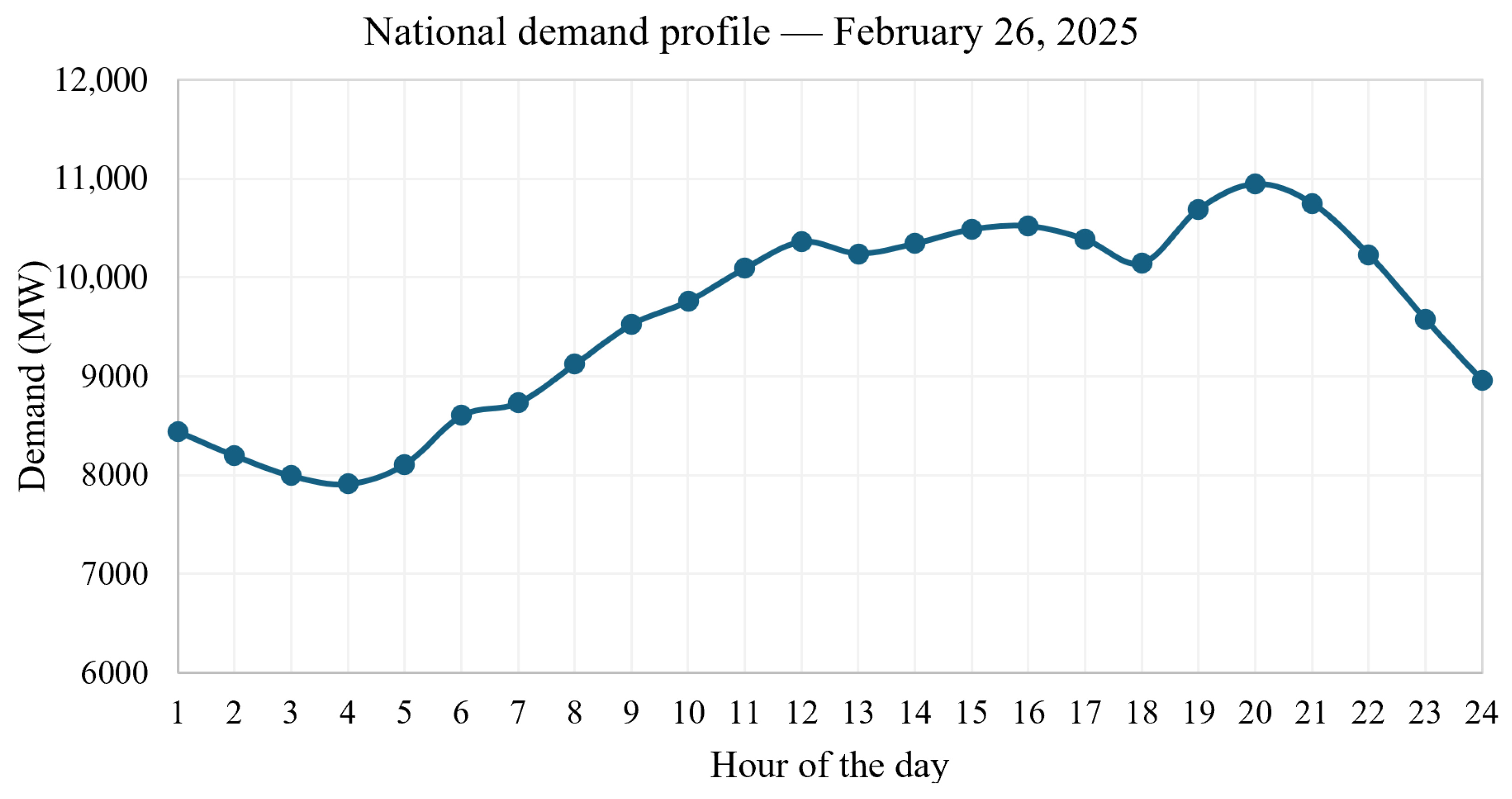
To adjust the load values for the demand at some hour of the day in the curve of the national power demand profile , consider the following procedure:
- 1.
- Disconnect the 115 kV network and voltage below from the 500, 230, and 220 kV network.
- 2.
- Identify the bus id of all 230/115 kV transformers in the network.
- 3.
- For each bus, replace each transformer with a load.
- 4.
- Calculates each load value in this way:
After assigning loads, we identify that an average demand of 10,500 MW is approximately of the maximum transformer capacity. Load can be adjusted at different values. To run this analysis, we adjust the maximum value of each load to 78% in separate analyses by area and apply the following factors for the frequency analysis for the interconnected region. , , , , and . The loads are then allocated as follows:
Appendix C. Algorithms
| Algorithm A1 Procedure to create a subarea |
|
| Algorithm A2 Procedure to create inter-area connections |
|
| Algorithm A3 General procedure to assemble the national power network |
|
| Algorithm A4 Generation Integration and P-V Curve Analysis |
|
| Algorithm A5 Procedure for Q–V analysis |
|
| Algorithm A6 Procedure for critical time analysis |
|
| Algorithm A7 Procedure for contingency stability analysis |
|
Appendix D. Codes
Appendix D.1. Atlántico Power System 500 kV–230 kV
# subareas/atlantico.py
import pandapower as pp
import matplotlib.pyplot as plt

def crear_red_atlantico():
    net = pp.create_empty_network(f_hz=60, sn_mva=100)
    factor = 0.7
    # Buses 230 kV
    bus_termoflores220 = pp.create_bus(net, vn_kv=220, name="Termoflores 220kV")
    bus_nvabarranquilla220 = pp.create_bus(net, vn_kv=220, ...
    name="Nva. Barranquilla 220kV")
    bus_caracoli220 = pp.create_bus(net, vn_kv=220, name="Caracoli 220kV")
    bus_tebsa220 = pp.create_bus(net, vn_kv=220, name="Tebsa 220kV")
    bus_sabanalarga220 = pp.create_bus(net, vn_kv=220, name="Sabanalarga 220kV")
    bus_elrio220 = pp.create_bus(net, vn_kv=220, name="El Rio 220kV")
   # bus_bolivar230=pp.create_bus(net,vn_kv=230,name="Bolivar 230kV")
    bus_termoflores230 = pp.create_bus(net,vn_kv=220, name="Bolivar 220kV")

    # Buses 500 kV principales
    bus_sabanalarga500 = pp.create_bus(net, vn_kv=500, name="Sabanalarga  500kV")
    bus_martillo500 = pp.create_bus(net, vn_kv=500, name="Martillo 500kV")
    #bus_chinu500=pp.create_bus(net,vn_kv=500, name="Chinu 500")

    # Líneas 500 kV (conexión externa)

    # Líneas 500 kV
    pp.create_line_from_parameters(net, bus_martillo500, bus_sabanalarga500, ...
    ...length_km=9.722, r_ohm_per_km=0.0251, x_ohm_per_km=0.319, c_nf_per_km=0, ...
    ...g_us_per_km=5.1032, max_i_ka=2.400, type= "ol", name="Martillo-Sabanalarga ...
    1 500kV")

    # Líneas 230kV

    pp.create_line_from_parameters(net, bus_caracoli220, bus_nvabarranquilla220, ...
    ...length_km=13.71, r_ohm_per_km=0.0802, x_ohm_per_km=0.486, c_nf_per_km=0,
    g_us_per_km=3.4082, max_i_ka=0.839,  type= "ol", name="Caracoli-Nueva ...
    ...Barranquilla 1 230kV")
    pp.create_line_from_parameters(net, bus_caracoli220, bus_sabanalarga220, ...
    length_km=30.29, r_ohm_per_km=0.0581, x_ohm_per_km=0.3658, c_nf_per_km=0, ...
    ... g_us_per_km=4.5829, max_i_ka=1.000,  type= "ol", name="Caracoli- ...
    Sabanalarga 230kV")
    pp.create_line_from_parameters(net, bus_caracoli220, bus_tebsa220, ...
    length_km=10.14, r_ohm_per_km=0.0796, x_ohm_per_km=0.4834, c_nf_per_km=0, ...
    g_us_per_km=3.4332, max_i_ka=0.839,  type= "ol", name="Caracoli-Tebsa 1 230kV")
    pp.create_line_from_parameters(net, bus_caracoli220, bus_termoflores220, ...
    length_km=35.9, r_ohm_per_km=0.052, x_ohm_per_km=0.3376, c_nf_per_km=0, ...
    g_us_per_km=3.4332, max_i_ka=0.839,  type= "ol", name="Caracoli-Tebsa 1 230kV")
    pp.create_line_from_parameters(net, bus_sabanalarga220, bus_tebsa220,  ...
    length_km=38.42, r_ohm_per_km=0.0897, x_ohm_per_km=0.496, c_nf_per_km=0, ...
    g_us_per_km=3.3541, max_i_ka=0.839,  type= "ol", name="Sabanalarga-Tebsa 1 ...
    230kV")
    pp.create_line_from_parameters(net, bus_sabanalarga220, bus_tebsa220,  ...
    length_km=38.42, r_ohm_per_km=0.0897, x_ohm_per_km=0.496, c_nf_per_km=0, ...
    g_us_per_km=3.3541, max_i_ka=0.839,  type= "ol", name="Sabanalarga-Tebsa 2...
    230kV")
    pp.create_line_from_parameters(net, bus_sabanalarga220, bus_tebsa220, ...
    length_km=38.42, r_ohm_per_km=0.0897, x_ohm_per_km=0.496, c_nf_per_km=0, ...
    g_us_per_km=3.3541, max_i_ka=0.839,  type= "ol", name="Sabanalarga-Tebsa 3 230kV")
    pp.create_line_from_parameters(net, bus_termoflores220, bus_nvabarranquilla220, ...
    length_km=7.4, r_ohm_per_km=0.0885, x_ohm_per_km=0.4658, c_nf_per_km=0, ...
    g_us_per_km=3.5795, max_i_ka=0.890,  type= "ol", name="Termoflores-Nueva ...
    ...Barranquilla 1 230kV")
    pp.create_line_from_parameters(net, bus_termoflores220, bus_nvabarranquilla220, ...
    length_km=7.4, r_ohm_per_km=0.0885, x_ohm_per_km=0.4658, c_nf_per_km=0, ...
    g_us_per_km=3.5795, max_i_ka=0.890,  type= "ol", name="Termoflores-...
    Nueva Barranquilla 2 230kV")
    pp.create_line_from_parameters(net, bus_nvabarranquilla220, bus_sabanalarga220, ...
    length_km=45.28, r_ohm_per_km=0.0818, x_ohm_per_km=0.4934, c_nf_per_km=0, ...
    g_us_per_km=3.3537, max_i_ka=0.839,  type= "ol",...
    ...name="Nueva Barranquilla-Sabanalarga 1  230kV")
    pp.create_line_from_parameters(net, bus_nvabarranquilla220, bus_sabanalarga220, ...
    length_km=45.28, r_ohm_per_km=0.0818, x_ohm_per_km=0.4934, c_nf_per_km=0, ...
    g_us_per_km=3.3537, max_i_ka=0.839,  type= "ol", name="Nueva Barranquilla ...
    ... -Sabanalarga 2 230kV")
    pp.create_line_from_parameters(net, bus_nvabarranquilla220, bus_sabanalarga220, ...
    length_km=45.28, r_ohm_per_km=0.0818, x_ohm_per_km=0.4934, c_nf_per_km=0, ...
    g_us_per_km=3.3537, max_i_ka=0.839,  type= "ol", name="Nueva Barranquilla...
    ...-Sabanalarga 3 230kV")
    pp.create_line_from_parameters(net, bus_elrio220, bus_termoflores230, ...
    length_km=45.28, r_ohm_per_km=0.0818, x_ohm_per_km=0.4934, c_nf_per_km=0, ...
    g_us_per_km=3.3537, max_i_ka=0.839,  type= "ol", name="Nueva Barranquilla-...
    ...Sabanalarga 3 230kV")
    pp.create_line_from_parameters(net, bus_elrio220, bus_tebsa220, ...
    length_km=7.37, r_ohm_per_km=0.0882, x_ohm_per_km=0.1348, c_nf_per_km=0, ...
    g_us_per_km=94.53, max_i_ka=1.306,  type= "ol", name="Nueva Barranquilla-...
    ...Sabanalarga 3 230kV")

    # Generadores

    pp.create_gen(net, bus_caracoli220, p_mw=47.5, vm_pu=1.0, name="Caracolí Solar")
    pp.create_gen(net, bus_martillo500, p_mw=541.5, vm_pu=1.0, name="Guayepo Solar")
    pp.create_gen(net, bus_tebsa220, p_mw=978.5, vm_pu=1.0, name="Tebsa")
    pp.create_gen(net, bus_termoflores220, p_mw=422.75, vm_pu=1.0, name="Flores ...
    ... IV CC")

    # Transformadores
    pp.create_transformer_from_parameters(net, bus_sabanalarga500, ...
    ...bus_sabanalarga220, sn_mva=1350, vn_hv_kv=500, vn_lv_kv=220, ...
    ...vk_percent=11.46, vkr_percent=0.5, i0_percent=0.1, pfe_kw=150, ...
    shift_degree=0, name="Trafo Sabanalarga 1350MVA")

    # Cargas resumidas (Barranquilla es gran centro de carga)
    pp.create_load(net, bus_sabanalarga220, p_mw=factor*171, q_mvar=factor*9, ...
    ...name="Carga Sabanalarga 230kV")
    pp.create_load(net, bus_caracoli220, p_mw=factor*285, q_mvar=factor*15,...
    ...name="Carga Caracoli 230kV")
    pp.create_load(net, bus_nvabarranquilla220, p_mw=factor*190, ...
    ...q_mvar=factor*10, name="Carga Nva Barranquilla 230kV")
    pp.create_load(net, bus_tebsa220, p_mw=factor*285, q_mvar=factor*15, ...
    ...name="Carga Tebsa 230kV")
    pp.create_load(net, bus_termoflores220, p_mw=factor*285, ...
    ...q_mvar=factor*15, name="Carga Termoflores 230kV")

    # Slack temporal
    #pp.create_ext_grid(net, bus_termoflores230, vm_pu=1.0, ...
    ...name="Slack Atlántico")

    return net# -*- coding: utf-8 -*-

"""
Created on Sat Jan 24 21:11:02 2026
Updated on Tur Feb 26 18:18:00 2026
Updated on Sat Feb 28 19:54:00 2026
@author: Claudia Caro
"""
Appendix D.2. Bolivar Power System 500 kV–230 kV
# subareas/bolivar.py
import pandapower as pp

def crear_red_bolivar():
    net = pp.create_empty_network(f_hz=60, sn_mva=100)
    factor = 0.78
    # Buses 500 kV
    bus_bolivar500 = pp.create_bus(net, vn_kv=500, name="Bolivar 500kV")
  #  bus_elcopey500 = pp.create_bus(net, vn_kv=500, name="El Copey 500kV")
 #   bus_sabanalarga500 = pp.create_bus(net, vn_kv=500, name="Sabanalarga 500kV")
    # Buses 220 kV
    bus_bolivar230 = pp.create_bus(net, vn_kv=230, name="Bolivar 230kV")
    bus_termocandelaria220 = pp.create_bus(net, vn_kv=220, name=...
    ..."Termocandelaria ...
    ... 220kV")
    bus_ternera220 = pp.create_bus(net, vn_kv=220, name="Ternera 220kV")
    bus_elbosque220 = pp.create_bus(net, vn_kv=220, name="El Bosque 220kV")
    bus_cartagena220 = pp.create_bus(net, vn_kv=220, name="Cartagena 220kV")
    #bus_sabanalarga230=pp.create_bus(net, vn_kv=230, name="Sabanalarga 230kV")
    # Líneas 500 kV (conexión externa)

    #pp.create_line_from_parameters(net, bus_bolivar500, bus_elcopey500, ...
    ...length_km=166.68, r_ohm_per_km=0.0237, x_ohm_per_km=0.3342, c_nf_per_km=0, ...
    ...g_us_per_km=4.9138, max_i_ka=2.476, type= "ol", name="Bolivar- ...
    El Copey 1 500kV")
   # pp.create_line_from_parameters(net, bus_bolivar500, bus_sabanalarga500, ...
   ...length_km=66.556, r_ohm_per_km=0.0239, x_ohm_per_km=0.3183, c_nf_per_km=0, ...
   ... g_us_per_km=5.1626, max_i_ka=3.120, type= "ol", name="Bolivar-Sabanalarga ...
   ... 1 500kV")

    pp.create_line_from_parameters(net, bus_cartagena220, bus_termocandelaria220, ...
    ...length_km=2.88, r_ohm_per_km=0.0892, x_ohm_per_km=0.4973, c_nf_per_km=0, ...
    ... g_us_per_km=3.3444, max_i_ka=0.813, type= "ol", name="Cartagena- ...
    ... Termocandelaria 1 230kV")
    pp.create_line_from_parameters(net, bus_cartagena220, bus_termocandelaria220, ...
    ...length_km=2.88, r_ohm_per_km=0.0892, x_ohm_per_km=0.4973, c_nf_per_km=0, ...
    ... g_us_per_km=3.3444, max_i_ka=0.813, type= "ol", name="Cartagena-...
    ...Termocandelaria 2 230kV")

    pp.create_line_from_parameters(net, bus_termocandelaria220, bus_ternera220, ...
    ...length_km=3.12, r_ohm_per_km=0.0896, x_ohm_per_km=0.4955, c_nf_per_km=0, ...
    ... g_us_per_km=3.3608, max_i_ka=0.813, type= "ol", name="Termocandelaria-...
    ...Ternera 1 230kV")
    pp.create_line_from_parameters(net, bus_termocandelaria220, bus_ternera220, ...
    ...length_km=3.12, r_ohm_per_km=0.0896, x_ohm_per_km=0.4955, c_nf_per_km=0, ...
    ... g_us_per_km=3.3608, max_i_ka=0.813, type= "ol", name="Termocandelaria-...
    ...Ternera 1 230kV")

    pp.create_line_from_parameters(net, bus_elbosque220, bus_ternera220, ...
    ...length_km=25.69, r_ohm_per_km=0.0602, x_ohm_per_km=0.452, c_nf_per_km=0, ...
    ... g_us_per_km=13.5127, max_i_ka=0.830, type= "ol", name="El Bosque-...
    ... Ternera 1 230kV")
  #  pp.create_line_from_parameters(net, bus_sabanalarga230, bus_ternera230, ...
  ...length_km=80.18, r_ohm_per_km=0.0893, x_ohm_per_km=0.496, c_nf_per_km=0, ...
  ... g_us_per_km=3.3541, max_i_ka=0.813, type= "ol", name="Sabanalarga-...
  ...Ternera 1 230kV")


    # Líneas 220 kV
    pp.create_line_from_parameters(net, bus_bolivar230, bus_elbosque220, ...
    ...length_km=17.29, r_ohm_per_km=0.049, x_ohm_per_km=0.384, c_nf_per_km=0, ...
    ...g_us_per_km=18.445, max_i_ka=0.800, type= "ol", name="Bolivar-...
    ...El Bosque 1 230kV")
    pp.create_line_from_parameters(net, bus_bolivar230, bus_cartagena220, ...
    ...length_km=18.3, r_ohm_per_km=0.063, x_ohm_per_km=0.491, c_nf_per_km=0, ...
    ...g_us_per_km=3.371, max_i_ka=0.929, type= "ol", name="Bolivar-...
    ...Cartagena 1 230kV")
    pp.create_line_from_parameters(net, bus_bolivar230, bus_cartagena220, ...
    ...length_km=18.3, r_ohm_per_km=0.063, x_ohm_per_km=0.491, c_nf_per_km=0, ...
    ...g_us_per_km=3.371, max_i_ka=0.929, type= "ol", name="Bolivar-...
    ... Cartagena 2 230kV")

    # Transformadores
    pp.create_transformer_from_parameters(net, bus_bolivar500, bus_bolivar230, ...
    ... sn_mva=900, vn_hv_kv=500, vn_lv_kv=230, vk_percent=11.71, vkr_percent=0.5,...
    ... i0_percent=0.1, pfe_kw=150, shift_degree=0, name="Trafo Bolivar 900MVA")

    # Generadores
    pp.create_gen(net, bus_termocandelaria220, p_mw=659.3, vm_pu=1.0, ...
    ...name="Termocandelaria")
    pp.create_gen(net, bus_cartagena220, p_mw=222.3, vm_pu=1.0, name="Cartagena")


    # Cargas resumidas (Cartagena es gran centro industrial)
    pp.create_load(net, bus_cartagena220, p_mw=factor*237.5, q_mvar=factor*12.5, ...
    ...name="Carga Cartagena 230kV")
    pp.create_load(net, bus_ternera220, p_mw=factor*399, q_mvar=factor*21, ...
    ...name="Carga Ternera 230kV")
    pp.create_load(net, bus_elbosque220, p_mw=factor*427.5, q_mvar=factor*22.5, ...
    ...name="Carga El Bosque 230kV")
    pp.create_load(net, bus_bolivar230, p_mw=factor*190, q_mvar=factor*10, ...
    ...name="Carga Bolivar 230kV")
    pp.create_load(net, bus_termocandelaria220, p_mw=factor*237.5,...
    ...q_mvar=factor*12.5, ...
    name="Carga Termocandelaria 230kV")

    # Slack temporal
   # pp.create_ext_grid(net, bus_bolivar500, vm_pu=1.0, name="Slack Bolívar")

    return net# -*- coding: utf-8 -*-


"""
Created on Sat Jan 24 21:10:43 2026
Updated on Tue Feb 24 22:32:00 2026
Updated on sat Feb 28 19:54:00 2026

@author: Claudia Caro
"""
Appendix D.3. Guajira-Cesar-Magdalena Power System 500 kV–230 kV
# subareas/gcm.py
import pandapower as pp
import matplotlib.pyplot as plt

def crear_red_gcm():
    net = pp.create_empty_network(f_hz=60, sn_mva=100)
    factor = 0.78
    # Buses 500 kV
    bus_laloma500 = pp.create_bus(net, vn_kv=500, name="La Loma 500kV")
    bus_elcopey500 = pp.create_bus(net, vn_kv=500, name="El Copey 500kV")
    bus_nuevacuestecitas500 = pp.create_bus(net, vn_kv=500, name="Nueva ...
    ...Cuestecitas 500kV")
    #bus_ocana500 = pp.create_bus(net, vn_kv=500, name="Nueva Cuestecitas 500kV")
    # Buses 230 kV
    bus_fundacion220 = pp.create_bus(net, vn_kv=220, name="Fundación 220kV")
    bus_riocordoba220 = pp.create_bus(net, vn_kv=220, name="Río Córdoba 220kV")
    bus_santamarta220 = pp.create_bus(net, vn_kv=220, name="Santa Marta 220kV")
    bus_termocol220 = pp.create_bus(net, vn_kv=220, name="Termocol 220kV")
    bus_guajira220 = pp.create_bus(net, vn_kv=220, name="Santa Marta 220kV")
    bus_cuestecitas220 = pp.create_bus(net, vn_kv=220, name="Cuestecitas 220kV")
    bus_nuevacuestecitas220 = pp.create_bus(net, vn_kv=220, name="Nueva ...
    ...Cuestecitas 220kV")
    bus_sanjuangeb220 = pp.create_bus(net, vn_kv=220, name="San Juan (GEB) 220kV")
    bus_valledupar220 = pp.create_bus(net, vn_kv=220, name="Valledupar 220kV")
    bus_elcopey220 = pp.create_bus(net, vn_kv=220, name="San Juan (GEB) 220kV")
   # bus_sabanalarga230 = pp.create_bus(net, vn_kv=230, name="Sabanalarga 230kV")


    # Líneas 500 kV
    pp.create_line_from_parameters(net, bus_elcopey500, ...
    ...bus_nuevacuestecitas500, ...
    ... length_km=218.292, r_ohm_per_km=0.0209, x_ohm_per_km=0.3095, ...
    ... c_nf_per_km=0, g_us_per_km=5.2587, max_i_ka=2.4, type= "ol", ...
    ... name="El Copey-Nueva Cuestecitas 1 500kV")
    pp.create_line_from_parameters(net, bus_elcopey500, bus_nuevacuestecitas500, ...
    ... length_km=218.292, r_ohm_per_km=0.0209, x_ohm_per_km=0.3095, ...
    ... c_nf_per_km=0, g_us_per_km=5.2587, max_i_ka=2.4, type= "ol", ...
    ... name="El Copey-Nueva Cuestecitas 2 500kV")
    pp.create_line_from_parameters(net, bus_elcopey500, bus_laloma500, ...
    ... length_km=73, r_ohm_per_km=0.016, x_ohm_per_km=0.356, ...
    ... c_nf_per_km=0, g_us_per_km=4.9138, max_i_ka=2.476,  type= "ol", ...
    ... name="El Copey-la Loma 1 500kV")
  #  pp.create_line_from_parameters(net, bus_laloma500, bus_ocana500, ...
  ... length_km=168, r_ohm_per_km=0.016, x_ohm_per_km=0.356, ...
  ... c_nf_per_km=0, g_us_per_km=4.9138, max_i_ka=2.476,  ...
  ... type= "ol",name="la Loma-Ocana 1 500kV")


    # Líneas 230 kV
    pp.create_line_from_parameters(net, bus_elcopey220, bus_fundacion220, ...
    ... length_km=50.237, r_ohm_per_km=0.0585, x_ohm_per_km=0.3645, ...
    ... c_nf_per_km=0, g_us_per_km=4.5474, max_i_ka=1.195,  type= "ol", ...
    ... name="El Copey-Fundación 2 230kV")
    pp.create_line_from_parameters(net, bus_elcopey220, bus_fundacion220, ...
    ... length_km=49.91, ... r_ohm_per_km=0.0897, x_ohm_per_km=0.5157, ...
    ... c_nf_per_km=0, g_us_per_km=3.2292, max_i_ka=0.815,  type= "ol", ...
    name="El Copey-Fundación 1 230kV")

    #pp.create_line_from_parameters(net, bus_fundacion230, bus_sabanalarga230, ...
    ... length_km=93.5, r_ohm_per_km=0.0897, x_ohm_per_km=0.5157, c_nf_per_km=0, ...
    ... g_us_per_km=3.2249, max_i_ka=0.813,  type= "ol", name="Fundacion-...
    ... Sabanalarga 1 230kV")
    #pp.create_line_from_parameters(net, bus_fundacion230, bus_sabanalarga230, ...
    ... length_km=91.15, r_ohm_per_km=0.0896, x_ohm_per_km=0.496, c_nf_per_km=0, ...
    ... g_us_per_km=3.3609, max_i_ka=0.988,  type= "ol", name="Fundacion-...
    ... Sabanalarga 2 230kV")
    #pp.create_line_from_parameters(net, bus_fundacion230, bus_sabanalarga230, ...
    ... length_km=91.2, r_ohm_per_km=0.0896, x_ohm_per_km=0.496, c_nf_per_km=0, ...
    ... g_us_per_km=3.3609, max_i_ka=0.957,  type= "ol", name="Fundacion-...
    ... Sabanalarga 3 230kV")


    pp.create_line_from_parameters(net, bus_fundacion220, bus_riocordoba220, ...
    ... length_km=62.56, r_ohm_per_km=0.074, x_ohm_per_km=0.4878, ...
    c_nf_per_km=0, g_us_per_km=3.379, max_i_ka=0.813,  ...
    type= "ol", name="Fundación-Rio Córdoba 1 230kV")
    pp.create_line_from_parameters(net, bus_fundacion220, bus_riocordoba220, ...
    ... length_km=62.56, r_ohm_per_km=0.074, x_ohm_per_km=0.4878, c_nf_per_km=0, ...
    ... g_us_per_km=3.379, max_i_ka=0.656,  type= "ol", name="Fundación-Rio ...
    ... Córdoba 2 230kV")

    pp.create_line_from_parameters(net, bus_cuestecitas220, bus_guajira220, ...
    ... length_km=95.45, r_ohm_per_km=0.0897, x_ohm_per_km=0.4911, ...
    ... c_nf_per_km=0, g_us_per_km=3.3929, max_i_ka=0.813,  type= "ol", ...
    ... name="Cuestecitas-Guajira 1 230kV")
    pp.create_line_from_parameters(net, bus_cuestecitas220, bus_guajira220, ...
    ... length_km=95.45, r_ohm_per_km=0.0897, x_ohm_per_km=0.4911, c_nf_per_km=0, ...
    g_us_per_km=3.3929, max_i_ka=0.813,  type= "ol", name="Cuestecitas-...
    ... Guajira 2 230kV")

    pp.create_line_from_parameters(net, bus_guajira220, bus_santamarta220, ...
    ... length_km=91.51, r_ohm_per_km=0.0897, x_ohm_per_km=0.4935, c_nf_per_km=0, ...
    ... g_us_per_km=3.3982, max_i_ka=0.813,  type= "ol", name="Guajira- ...
    ... Santa Marta 2 230kV")
    pp.create_line_from_parameters(net, bus_guajira220, bus_termocol220, ...
    ... length_km=81.47, r_ohm_per_km=0.0896, x_ohm_per_km=0.4935, c_nf_per_km=0, ...
    ... g_us_per_km=3.32, max_i_ka=0.813,  type= "ol", name="Guajira-Termocol 1 ...
    ... 230kV")

    pp.create_line_from_parameters(net, bus_elcopey220, bus_valledupar220, ...
    ... length_km=90.8, r_ohm_per_km=0.0897, x_ohm_per_km=0.5157, c_nf_per_km=0, ...
    ... g_us_per_km=3.2292, max_i_ka=0.818,  type= "ol", name="El Copey- ...
    ... Valleduoar 1 ...
    ... 230kV")
    pp.create_line_from_parameters(net, bus_elcopey220, bus_valledupar220, ...
    ... length_km=96.13, r_ohm_per_km=0.073, x_ohm_per_km=0.497, c_nf_per_km=0, ...
    ... g_us_per_km=3.3032, max_i_ka=0.588,  type= "ol", name="El Copey ...
    ... -Valleduoar 2 230kV")

    pp.create_line_from_parameters(net, bus_santamarta220, bus_termocol220, ...
    ... length_km=11.56, r_ohm_per_km=0.0887, x_ohm_per_km=0.5157, c_nf_per_km=0, ...
    ... g_us_per_km=3.2292, max_i_ka=0.813,  type= "ol", name="Santa Marta- ...
    ... Termocol 1 230kV")
    pp.create_line_from_parameters(net, bus_riocordoba220, bus_santamarta220, ...
    ... length_km=22.39, r_ohm_per_km=0.0737, x_ohm_per_km=0.4877, c_nf_per_km=0, ...
    ... g_us_per_km=3.379, max_i_ka=0.813,  type= "ol", name="Rio Córdoba-Santa ...
    ... Marta 1 230kV")
    pp.create_line_from_parameters(net, bus_riocordoba220, bus_santamarta220, ...
    ... length_km=22.38, r_ohm_per_km=0.0737, x_ohm_per_km=0.4877, c_nf_per_km=0, ...
    ... g_us_per_km=3.379, max_i_ka=0.656,  type= "ol", name="Rio Córdoba-...
    ... Santa Marta 2 230kV")

    pp.create_line_from_parameters(net, bus_sanjuangeb220, bus_valledupar220, ...
    ... length_km=51.57, r_ohm_per_km=0.0664, x_ohm_per_km=0.4988, c_nf_per_km=0, ...
    ... g_us_per_km=3.2406, max_i_ka=0.656,  type= "ol", name="San Juan (GEB)- ...
    ... Valledupar 230kV")
    pp.create_line_from_parameters(net, bus_cuestecitas220, bus_sanjuangeb220, ...
    ... length_km=70.22, r_ohm_per_km=0.0675, x_ohm_per_km=0.506, c_nf_per_km=0, ...
    ... g_us_per_km=3.2795, max_i_ka=0.813,  type= "ol", name="Cuestecitas- ...
    ... San Juan (GEB) 230kV")

    pp.create_line_from_parameters(net, bus_cuestecitas220, bus_nuevacuestecitas220, ...
    ... length_km=2, r_ohm_per_km=0.0303, x_ohm_per_km=0.3514, c_nf_per_km=0, ...
    ... g_us_per_km=4.7244, max_i_ka=2.000,  type= "ol", name="Cuestecitas- ...
    ... Nueva Cuestecitas 1 230kV")

    # Transformadores
    pp.create_transformer_from_parameters(net, bus_elcopey500, bus_elcopey220, ...
    ... sn_mva=900, vn_hv_kv=500,vn_lv_kv=220, vk_percent=11.47, vkr_percent=0.5,...
    ... i0_percent=0.1, pfe_kw=150, shift_degree=0, name="Trafo El Copey 900MVA")
    pp.create_transformer_from_parameters(net, bus_nuevacuestecitas500, ...
    bus_nuevacuestecitas220, sn_mva=450, vn_hv_kv=500,vn_lv_kv=220, vk_percent=11.3, ...
    ... vkr_percent=0.5, i0_percent=0.1, pfe_kw=150, shift_degree=0, ...
    ...name="Trafo Cuestecitas 450MVA")

    # Generación

    pp.create_gen(net, bus_termocol220, p_mw=118.75, vm_pu=1.0, name="Termonorte")
    pp.create_gen(net, bus_guajira220, p_mw=456, vm_pu=1.0, name="Guajira")

    # Cargas resumidas
    pp.create_load(net, bus_laloma500, p_mw=factor*285, q_mvar=factor*15, ...
    ... name="Carga La Loma 500kV")
    pp.create_load(net, bus_elcopey220, p_mw=factor*190, q_mvar=factor*10, ...
    ... name="Carga EL Copey 230kV")
    pp.create_load(net, bus_valledupar220, p_mw=factor*190, q_mvar=factor*10, ...
    ... name="Carga Valledupar 230kV")
    pp.create_load(net, bus_santamarta220, p_mw=factor*285, q_mvar=factor*15, ...
    ... name="Carga Santa Marta 230kV")
    pp.create_load(net, bus_riocordoba220, p_mw=factor*190, q_mvar=factor*10, ...
    ... name="Carga Rio Córdoba 230kV")
    pp.create_load(net, bus_fundacion220, p_mw=factor*147.25, q_mvar=factor*12.5, ...
    ... name="Carga Fundación 230kV")
    pp.create_load(net, bus_cuestecitas220, p_mw=factor*285, q_mvar=factor*15, ...
    ... name="Carga Cuestecitas 230kV")


    # Slack temporal
   # pp.create_ext_grid(net, bus_laloma500, vm_pu=1.0, name="Slack GCM")

    return net# -*- coding: utf-8 -*-


"""
Created on Sat Jan 24 21:15:01 2026

@author: Claudia Caro
"""


"""
Updated on Tur Feb 26 22:34:39 2026

Updated on Sat Feb 28 19:25:00 19:25:00 2026

@author: Claudia Caro
"""
Appendix D.4. Cerromatoso Power System 500 kV–230 kV
# subareas/cerromatoso.py
import pandapower as pp

def crear_red_cerromatoso():
    net = pp.create_empty_network(f_hz=60, sn_mva=100)
    factor = 0.78
    # Buses 500 kV
    bus_cerromatoso500 = pp.create_bus(net, vn_kv=500, name="Cerromatoso 500kV")
    #bus_chinu500 = pp.create_bus(net, vn_kv=500, name="Chinú 500kV")
    #bus_sahagun500 = pp.create_bus(net, vn_kv=500, name="Sahagun 500kV")
    #bus_porceiii500 = pp.create_bus(net, vn_kv=500, name="Porce III 500kV")
    #bus_primavera500 = pp.create_bus(net, vn_kv=500, name="Primavera 500kV")

    # Buses 230 kV
    bus_cerromatoso230 = pp.create_bus(net, vn_kv=230, name="Cerromatoso 230kV")
    #bus_urra230=pp.create_bus(net, vn_kv=230, name="Urrá 230kV")


    # Líneas 500 kV (conexión externa)

    # Líneas 230 kV
   # pp.create_line_from_parameters(net, bus_cerromatoso500, bus_chinu500,...
   ...length_km=136.3, r_ohm_per_km=0.0281, x_ohm_per_km=0.3116, ...
   ... c_nf_per_km=0, g_us_per_km=3.4996, max_i_ka=2.4, type= "ol", ...
   ... name="Cerromatoso-Chinú 3 500kV")
   # pp.create_line_from_parameters(net, bus_cerromatoso500, bus_porceiii500,...
   ...length_km=141.65, r_ohm_per_km=0.0262, x_ohm_per_km=0.33, c_nf_per_km=0, ...
   ... g_us_per_km=3.4996, max_i_ka=2.0, type= "ol", name="Cerromatoso-...
   ... Porce III 1 500kV")
   # pp.create_line_from_parameters(net, bus_cerromatoso500, bus_primavera500,...
   ...length_km=245.21, r_ohm_per_km=0.0247, x_ohm_per_km=0.3227, c_nf_per_km=0,
   ... g_us_per_km=5.1337, max_i_ka=2.0, type= "ol", name="Cerromatoso-...
   ... Primavera 1 500kV")
   # pp.create_line_from_parameters(net, bus_cerromatoso500, bus_sahagun500, ...
   ... length_km=79.1, r_ohm_per_km=0.0222, x_ohm_per_km=0.347, c_nf_per_km=0, ...
   ... g_us_per_km=4.8779, max_i_ka=2.449, type= "ol", name="Cerromatoso-...
   ... Sahagun 1 500kV")
   # pp.create_line_from_parameters(net, bus_cerromatoso230, bus_urra230,  ...
   ... length_km=84.61, r_ohm_per_km=0.0614, x_ohm_per_km=0.5175, c_nf_per_km=0, ...
   ... g_us_per_km=3.3504, max_i_ka=0.881, type= "ol", name="Cerromatoso-Urra ...
   ... 1 230kV")
   # pp.create_line_from_parameters(net, bus_cerromatoso230, bus_urra230, ...
   ... length_km=84.61, r_ohm_per_km=0.0614, x_ohm_per_km=0.5175, c_nf_per_km=0, ...
   ... g_us_per_km=3.3504, max_i_ka=0.881, type= "ol", name="Cerromatoso-Urra 2 ...
   ... 230kV")

    # Cargas resumidas
    pp.create_load(net, bus_cerromatoso500, p_mw=factor*427.5, q_mvar=factor*21.5,...
    ... name="Carga Cerromatoso 1 500kV")
    pp.create_load(net, bus_cerromatoso500, p_mw=factor*427.5, q_mvar=factor*21.5,...
    ... name="Carga Cerromatoso 2 500kV")

    # Transformadores
    pp.create_transformer_from_parameters(net, bus_cerromatoso500, ...
    ... bus_cerromatoso230, sn_mva=360, vn_hv_kv=500, vn_lv_kv=230, ...
    ... vk_percent=11.71, vkr_percent=0.5, i0_percent=0.1, pfe_kw=150, ...
    ... shift_degree=0,name="Trafo Cerromatoso 350MVA")

    # Slack temporal
    #pp.create_ext_grid(net, bus_cerromatoso500, vm_pu=1.0, name="Cerromatoso")

    return net# -*- coding: utf-8 -*-


"""
Spyder Editor

Created on Sat Jan 24 21:12:15 2026
Update 1 on Tue Feb 24 12:30 2026
Update 2 on Sat Feb 28 19:04:00 2026

@author: Claudia Caro

This is a temporary script file.
"""
Appendix D.5. P-V Analysis
# -*- coding: utf-8 -*-
"""
Created on Mon Mar 16 13:01:56 2026

@author: Claudia
"""

import pandapower as pp
import pandas as pd
import matplotlib.pyplot as plt
from red_nacional import crear_red_nacional

# Crear la red base
net = crear_red_nacional()

# 1. Añadir generadores ficticios en todos los buses (si no existen)
for bus_idx in net.bus.index:
    if not (net.gen.bus == bus_idx).any():  # si no hay gen en ese bus
        pp.create_gen(net, bus=bus_idx, p_mw=1.0, vm_pu=1.0)

# Guardar valores base de todos los generadores
base_gens = net.gen["p_mw"].copy()

# 2. Barrido de lambda para integración de generación
results = []
lambdas = [i * 0.05 for i in range(21)]

for lam in lambdas:
    # Escalar generación respecto al valor base
    for idx in net.gen.index:
        net.gen.at[idx, "p_mw"] = base_gens[idx] * (1 + lam)

    try:
        pp.runpp(net)
        res = {"lambda": lam}
        for bus_idx in net.bus.index:
            res[f"V_bus{bus_idx}"] = net.res_bus.vm_pu[bus_idx]
        results.append(res)
    except:
        print(f"No converge en lambda={lam}")
        break

df = pd.DataFrame(results)

# 3. Graficar curvas P–V de integración de generación
for bus_idx in net.bus.index:
    bus_name = net.bus.at[bus_idx, "name"] if "name" in net.bus.columns else...
    ... f"Bus {bus_idx}"
    subarea = net.bus.at[bus_idx, "subarea"] if "subarea" in net.bus.columns else ...
    ... "Sin subárea"
    etiqueta = f"{bus_name} ({subarea})"
    plt.plot(df["lambda"], df[f"V_bus{bus_idx}"], label=etiqueta)

plt.xlabel("Factor de incremento lambda")
plt.ylabel("Voltaje (pu)")
plt.title("Curvas P–V para integración de generación nueva")
plt.legend()
plt.grid(True)
plt.show()
Appendix D.6. Q-V Analysis Algorithm
# -*- coding: utf-8 -*-
"""
Created on Tue Mar 17 08:26:35 2026

@author: Claudia
"""

import pandapower as pp
import pandas as pd
import matplotlib.pyplot as plt
from red_nacional import crear_red_nacional

# Crear red base
net = crear_red_nacional()

# Definir potencia nominal ficticia de cada aerogenerador (ejemplo: 50 MW por nodo)
p_nominal = 250.0  # MW
q_max = 0.3 * p_nominal  # ±30% of Pnominal; approximately the typical Q-support range

# Crear generadores ficticios de reactivos (sgen con p=0)
for bus_idx in net.bus.index:
    if not (net.sgen.bus == bus_idx).any():
        pp.create_sgen(net, bus=bus_idx, p_mw=0.0, q_mvar=0.0)

# Rango de Q a explorar (ejemplo: -Qmax a +Qmax)
q_values = [i for i in range(int(-q_max), int(q_max)+10, 10)]

# Diccionario para guardar resultados
resultados_por_bus = {}

for bus_idx in net.bus.index:
    idx_sgen = net.sgen[net.sgen.bus == bus_idx].index[0]
    resultados = []
    for q in q_values:
        net.sgen.at[idx_sgen, "q_mvar"] = q
        try:
            pp.runpp(net)
            vm = net.res_bus.vm_pu[bus_idx]
            resultados.append({"Q (Mvar)": q, "V (pu)": vm})
        except:
            break
    resultados_por_bus[bus_idx] = pd.DataFrame(resultados)

# Exportar a Excel
with pd.ExcelWriter("curvas_QV_eolico.xlsx") as writer:
    # Guardar curvas por bus
    for bus_idx, df_qv in resultados_por_bus.items():
        bus_name = net.bus.at[bus_idx, "name"] if "name" in net.bus.columns ...
        ... else f"Bus {bus_idx}"
        subarea = net.bus.at[bus_idx, "subarea"] if "subarea" in net.bus.columns ...
        ... else "Córdoba-Sucre"
        hoja = f"{bus_name}_{subarea}"
        df_qv.to_excel(writer, sheet_name=hoja[:31], index=False)

    # Crear hoja resumen con Q límite
    resumen = []
    for bus_idx, df_qv in resultados_por_bus.items():
        bus_name = net.bus.at[bus_idx, "name"] if "name" in net.bus.columns ...
        ... else f"Bus {bus_idx}"
        subarea = net.bus.at[bus_idx, "subarea"] if "subarea" in net.bus.columns ...
        ... else "Córdoba-Sucre"
        limite = df_qv.loc[df_qv["V (pu)"] < 0.95, "Q (Mvar)"]
        if not limite.empty:
            q_limite = limite.iloc[0]
        else:
            q_limite = df_qv["Q (Mvar)"].max()
        resumen.append({"Bus": bus_name, "Subarea": subarea,
                        "Q base (Mvar)": 0.0,
                        "Q límite (Mvar)": q_limite,
                        "Rango recomendado (Mvar)": f"±{q_max:.1f}"})
    df_resumen = pd.DataFrame(resumen)
    df_resumen.to_excel(writer, sheet_name="Resumen", index=False)

# Graficar todas las curvas en una sola figura
plt.figure(figsize=(12,7))
for bus_idx, df_qv in resultados_por_bus.items():
    bus_name = net.bus.at[bus_idx, "name"] if "name" in net.bus.columns...
    ... else f"Bus {bus_idx}"
    subarea = net.bus.at[bus_idx, "subarea"] if "subarea" in net.bus.columns ...
    ... else "Córdoba-Sucre"
    etiqueta = f"{bus_name} ({subarea}) - Rango=±{q_max:.1f} Mvar"
    plt.plot(df_qv["Q (Mvar)"], df_qv["V (pu)"], marker="o", label=etiqueta)

    # Detectar límite de voltaje mínimo 0.95
    limite = df_qv.loc[df_qv["V (pu)"] < 0.95, "Q (Mvar)"]
    if not limite.empty:
        q_limite = limite.iloc[0]
        plt.axvline(x=q_limite, color="red", linestyle="--", alpha=0.5)
        plt.text(q_limite, 0.96, f"Q={q_limite:.1f}", rotation=90, color="red")

# Línea horizontal de referencia en 0.95 pu
plt.axhline(y=0.95, color="red", linestyle="--", alpha=0.7)
plt.text(q_max*0.7, 0.951, "Límite 0.95 pu", color="red")

plt.xlabel("Potencia reactiva Q (Mvar)")
plt.ylabel("Voltaje (pu)")
plt.title("Curvas Q–V de todos los buses con integración eólica")
plt.legend(fontsize=7, loc="upper center", bbox_to_anchor=(0.5, -0.15), ncol=3)
plt.grid(True)
plt.tight_layout()
plt.show()
Appendix D.7. Angle Stability Analysis
# -*- coding: utf-8 -*-
"""
Created on Tue Mar 17 15:45:58 2026

@author: Claudia
"""

import pandapower as pp
import pandas as pd
import matplotlib.pyplot as plt
from red_nacional import crear_red_nacional

# Crear red base
net = crear_red_nacional()

# Crear generadores ficticios en todos los buses (si no existen)
for bus_idx in net.bus.index:
    if not (net.sgen.bus == bus_idx).any():
        pp.create_sgen(net, bus=bus_idx, p_mw=110.0, q_mvar=0.0)

# Guardar valores base de los sgen
base_sgens = net.sgen["p_mw"].copy()

results = []
lambdas = [i*0.1 for i in range(21)]  # de 0 a 2.0

for lam in lambdas:
    # Escalar generación activa
    for idx in net.sgen.index:
        net.sgen.at[idx, "p_mw"] = base_sgens[idx] * (1 + lam)
    try:
        pp.runpp(net)
        res = {"lambda": lam}
        for bus_idx in net.bus.index:
            res[f"delta_bus{bus_idx}"] = net.res_bus.va_degree[bus_idx]
        results.append(res)
    except:
        print(f"No converge en lambda={lam}")
        break

df = pd.DataFrame(results)

# Exportar a Excel
with pd.ExcelWriter("estabilidad_angulo.xlsx") as writer:
    # Guardar curvas por bus
    for bus_idx in net.bus.index:
        bus_name = net.bus.at[bus_idx, "name"] if "name" in net.bus.columns...
        ...else f"Bus {bus_idx}"
        subarea = net.bus.at[bus_idx, "subarea"] if "subarea" in ...
        ...net.bus.columns else "Arauca"
        hoja = f"{bus_name}_{subarea}"
        df_bus = df[["lambda", f"delta_bus{bus_idx}"]]
        df_bus.to_excel(writer, sheet_name=hoja[:31], index=False)

    # Crear hoja resumen con lambda límite y potencia máxima integrable
    resumen = []
    for bus_idx in net.bus.index:
        bus_name = net.bus.at[bus_idx, "name"] if "name" in net.bus.columns...
        ... else f"Bus {bus_idx}"
        subarea = net.bus.at[bus_idx, "subarea"] if "subarea" in ...
        ...net.bus.columns else "Arauca"
        angulos = df[f"delta_bus{bus_idx}"]
        limite = df.loc[angulos >= 90, "lambda"]
        if not limite.empty:
            lam_limite = limite.iloc[0]
        else:
            lam_limite = df["lambda"].max()
        p_base = base_sgens[net.sgen[net.sgen.bus == bus_idx].index[0]]
        p_max = p_base * (1 + lam_limite)
        resumen.append({"Bus": bus_name, "Subarea": subarea,
                        "lambda límite": lam_limite, "Pmax (MW)": p_max})

    df_resumen = pd.DataFrame(resumen)
    df_resumen.to_excel(writer, sheet_name="Resumen", index=False)

# Graficar todas las curvas P–delta en una sola figura
plt.figure(figsize=(12,7))
for bus_idx in net.bus.index:
    bus_name = net.bus.at[bus_idx, "name"] if "name" in net.bus.columns else...
    ... f"Bus {bus_idx}"
    subarea = net.bus.at[bus_idx, "subarea"] if "subarea" in net.bus.columns...
    ... else "Arauca"
    etiqueta = f"{bus_name} ({subarea}) - Pbase={base_sgens[net.sgen[net.sgen.bus ...
    ... == bus_idx].index[0]]:.1f} MW"
    plt.plot(df["lambda"], df[f"delta_bus{bus_idx}"], label=etiqueta)

    # Detectar límite delta=90°
    limite = df.loc[df[f"delta_bus{bus_idx}"] >= 90, "lambda"]
    if not limite.empty:
        lam_limite = limite.iloc[0]
        plt.axvline(x=lam_limite, color="red", linestyle="--", alpha=0.5)
        plt.text(lam_limite, 91, f"lambda={lam_limite:.2f}", rotation=90, color="red")

plt.axhline(y=90, color="red", linestyle="--", alpha=0.7)
plt.text(df["lambda"].max()*0.8, 91, "Límite delta=90°", color="red")

plt.xlabel("Factor de incremento lambda")
plt.ylabel("Ángulo delta (grados)")
plt.title("Curvas P–delta (Estabilidad de ángulo) en todos los buses")
plt.legend(fontsize=7, loc="upper center", bbox_to_anchor=(0.5, -0.15), ncol=3)
plt.grid(True)
plt.tight_layout()
plt.show()
Appendix D.8. Frequency Stability Analysis
# -*- coding: utf-8 -*-
"""
Created on Tue Mar 17 21:27:27 2026

@author: Claudia
"""

import numpy as np
import pandas as pd
import matplotlib.pyplot as plt
import pandapower as pp
from pandapower.pypower.makeYbus import makeYbus
from red_nacional import crear_red_nacional

net = crear_red_nacional()

f0 = 60.0
omega_s = 2*np.pi*f0
t = np.linspace(0, 5, 1000)
dt = t[1]-t[0]

turbinas = {
    "DFIG (80m)": 2.5,
    "FullConv (120m, sin sintética)": 0.5,
    "FullConv (120m, con sintética)": 1.5,
    "Eje vertical (60m)": 0.8
}

potencias_nuevas = [20, 50, 100, 200]
P_ref = 10.0

resultados = []

for bus_idx in net.bus.index:
    bus_name = net.bus.at[bus_idx,"name"] if "name" in net.bus.columns else...
    ...f"Bus {bus_idx}"

    # Potencia nominal existente
    if (net.sgen.bus == bus_idx).any():
        p_nominal_base = net.sgen.loc[net.sgen.bus == bus_idx,"p_mw"].sum()
    else:
        p_nominal_base = 0.0

    for p_add in potencias_nuevas:
        # Añadir nueva generación ficticia en el bus
        sgen_idx = pp.create_sgen(net, bus=bus_idx, p_mw=p_add, name="Eolica_temp")
        pp.runpp(net)

        # Construir Ybus y calcular P_e actualizado
        Ybus, _, _ = makeYbus(net._ppc["baseMVA"], net._ppc["bus"],...
        ...net._ppc["branch"])
        Vm = net.res_bus["vm_pu"].values
        Va = np.deg2rad(net.res_bus["va_degree"].values)
        V = Vm * np.exp(1j*Va)
        I = Ybus.dot(V)
        P_e_all = np.real(V * np.conj(I)) * net.sn_mva
        P_e_base = float(P_e_all[bus_idx])

        p_nominal = p_nominal_base + p_add

        for tipo, H_base in turbinas.items():
            H = H_base * (p_nominal / P_ref) if p_nominal > 0 else H_base * 0.5

            delta = 0.0
            omega = omega_s
            delta_hist, omega_hist = [], []

            for _ in t:
                P_m = p_nominal
                P_e = P_e_base
                ddelta = omega - omega_s
                domega = (P_m - P_e)/(2*H)
                delta += ddelta*dt
                omega += domega*dt
                delta_hist.append(delta)
                omega_hist.append(omega)

            freq = np.array(omega_hist)/(2*np.pi)
            if np.any(freq < 59.5):
                tcd = t[np.where(freq < 59.5)[0][0]]
            elif np.any(np.array(delta_hist) > np.pi/2):
                tcd = t[np.where(np.array(delta_hist) > np.pi/2)[0][0]]
            else:
                tcd = t[-1]

            resultados.append({
                "Bus": bus_name,
                "Penetración (MW)": p_add,
                "Tipo turbina": tipo,
                "Tiempo crítico (s)": round(tcd,2)
            })

        # Eliminar el generador ficticio antes del siguiente escenario
        net.sgen.drop(sgen_idx, inplace=True)

df_resumen = pd.DataFrame(resultados)

# --- SUBPLOTS 2D ---
buses = df_resumen["Bus"].unique()
n_buses = len(buses)
n_cols = 3
n_rows = int(np.ceil(n_buses / n_cols))

fig, axes = plt.subplots(n_rows, n_cols, figsize=(15, 4*n_rows), sharey=True)

for i, bus_name in enumerate(buses):
    ax = axes.flat[i]
    subset = df_resumen[df_resumen["Bus"]==bus_name]
    for tipo in turbinas.keys():
        datos = subset[subset["Tipo turbina"]==tipo]
        ax.plot(datos["Penetración (MW)"], datos["Tiempo crítico (s)"], marker="o", label=tipo)
    ax.set_title(bus_name)
    ax.set_xlabel("Penetración nueva (MW)")
    ax.set_ylabel("Tiempo crítico (s)")
    ax.grid(True)
    ax.legend(fontsize=7)

plt.tight_layout()
plt.show()
# --- EXPORTAR A EXCEL ---
df_resumen.to_excel("tiempos_criticos_bogota_V20052026.xlsx", index=False)
Appendix D.9. Contingency Analysis
# -*- coding: utf-8 -*-
"""
Created on Tue Mar 17 23:07:44 2026

@author: Claudia
"""

import pandapower as pp
import pandapower.topology as top
import networkx as nx
import pandas as pd
import matplotlib.pyplot as plt
import numpy as np
from itertools import combinations
from red_nacional import crear_red_nacional
net = crear_red_nacional()
penetraciones = [200,  500, 1000, 1500]
resultados = []

def detectar_islas(net):
    G = top.create_nxgraph(net, include_lines=True, include_trafos=True)
    return list(nx.connected_components(G))

def clasificar(valor, criterio):
    if valor is None:
        return "Error"
    if criterio == "Voltaje (pu)":
        if 0.95 <= valor <= 1.05: return "Verde"
        elif 0.90 <= valor <= 1.10: return "Amarillo"
        else: return "Rojo"
    if criterio == "Ángulo (°)":
        if abs(valor) < 30: return "Verde"
        elif abs(valor) < 45: return "Amarillo"
        else: return "Rojo"
    if criterio == "Frecuencia (Hz)":
        if 59.8 <= valor <= 60.2: return "Verde"
        elif 59.5 <= valor <= 60.5: return "Amarillo"
        else: return "Rojo"
    if criterio == "Carga líneas (%)":
        if valor < 80: return "Verde"
        elif valor < 100: return "Amarillo"
        else: return "Rojo"
    return "Error"

# --- Simulación ---
for bus_idx in net.bus.index:
    bus_name = net.bus.at[bus_idx,"name"] if "name" in net.bus.columns else ...
    ...f"Bus {bus_idx}"

    for p_add in penetraciones:
        net_c = net.deepcopy()
        pp.create_sgen(net_c, bus=bus_idx, p_mw=p_add, name="Eolica_temp")

        try:
            pp.runpp(net_c)
            sobrecargadas = net_c.res_line[net_c.res_line.loading_percent >...
            ...100].index.tolist()
        except:
            sobrecargadas = []

        # Siempre generamos al menos un resultado base
        V = net_c.res_bus.vm_pu.mean() if hasattr(net_c, "res_bus") else None
        ang = net_c.res_bus.va_degree.mean() if hasattr(net_c, "res_bus") else None
        freq = 60 - (net_c.res_sgen.p_mw.sum() - net_c.res_load.p_mw.sum())*0.01 ...
        ...if hasattr(net_c, "res_sgen") else None
        load = net_c.res_line.loading_percent.mean() ...
        ...if hasattr(net_c, "res_line") else None

        resultados.append({
            "Tipo contingencia": "Base",
            "Bus generación": bus_name,
            "Penetración (MW)": p_add,
            "Líneas fuera": [],
            "Islas": str(detectar_islas(net_c)),
            "Voltaje (pu)": V,
            "Clasificación Voltaje": clasificar(V,"Voltaje (pu)"),
            "Ángulo (°)": ang,
            "Clasificación Ángulo": clasificar(ang,"Ángulo (°)"),
            "Frecuencia (Hz)": freq,
            "Clasificación Frecuencia": clasificar(freq,"Frecuencia (Hz)"),
            "Carga líneas (%)": load,
            "Clasificación Carga": clasificar(load,"Carga líneas (%)")
        })

        # Contingencias N-1
        for linea in sobrecargadas:
            net_n1 = net_c.deepcopy()
            net_n1.line.drop(linea, inplace=True)
            try:
                pp.runpp(net_n1)
                V = net_n1.res_bus.vm_pu.mean()
                ang = net_n1.res_bus.va_degree.mean()
                freq = 60 - (net_n1.res_sgen.p_mw.sum() -...
                ...net_n1.res_load.p_mw.sum())*0.01
                load = net_n1.res_line.loading_percent.mean()
                islas = detectar_islas(net_n1)
            except:
                V, ang, freq, load, islas = None, None, None, None, "Error"

            resultados.append({
                "Tipo contingencia": "N-1",
                "Bus generación": bus_name,
                "Penetración (MW)": p_add,
                "Líneas fuera": [linea],
                "Islas": str(islas),
                "Voltaje (pu)": V,
                "Clasificación Voltaje": clasificar(V,"Voltaje (pu)"),
                "Ángulo (°)": ang,
                "Clasificación Ángulo": clasificar(ang,"Ángulo (°)"),
                "Frecuencia (Hz)": freq,
                "Clasificación Frecuencia": clasificar(freq,"Frecuencia (Hz)"),
                "Carga líneas (%)": load,
                "Clasificación Carga": clasificar(load,"Carga líneas (%)")
            })

        # Contingencias N-2
        for linea1, linea2 in combinations(sobrecargadas, 2):
            net_n2 = net_c.deepcopy()
            net_n2.line.drop([linea1, linea2], inplace=True)
            try:
                pp.runpp(net_n2)
                V = net_n2.res_bus.vm_pu.mean()
                ang = net_n2.res_bus.va_degree.mean()
                freq = 60 - (net_n2.res_sgen.p_mw.sum() -...
                ...net_n2.res_load.p_mw.sum())*0.01
                load = net_n2.res_line.loading_percent.mean()
                islas = detectar_islas(net_n2)
            except:
                V, ang, freq, load, islas = None, None, None, None, "Error"

            resultados.append({
                "Tipo contingencia": "N-2",
                "Bus generación": bus_name,
                "Penetración (MW)": p_add,
                "Líneas fuera": [linea1, linea2],
                "Islas": str(islas),
                "Voltaje (pu)": V,
                "Clasificación Voltaje": clasificar(V,"Voltaje (pu)"),
                "Ángulo (°)": ang,
                "Clasificación Ángulo": clasificar(ang,"Ángulo (°)"),
                "Frecuencia (Hz)": freq,
                "Clasificación Frecuencia": clasificar(freq,"Frecuencia (Hz)"),
                "Carga líneas (%)": load,
                "Clasificación Carga": clasificar(load,"Carga líneas (%)")
            })

# Exportar resultados
df_resumen = pd.DataFrame(resultados)
df_resumen.to_excel("contingencias_n1_n2_eolica_clasificado.xlsx", index=False)

## --- Heatmap con Matplotlib en subplots por penetración ---
mapa_valores = {"Verde": 0, "Amarillo": 1, "Rojo": 2, "Error": -1}
criterios = ["Clasificación Voltaje", "Clasificación Ángulo",
             "Clasificación Frecuencia", "Clasificación Carga"]

df_heatmap = df_resumen.copy()
for criterio in criterios:
    if criterio in df_heatmap.columns:
        df_heatmap[criterio] = df_heatmap[criterio].map(mapa_valores)

# Niveles de penetración únicos
niveles = sorted(df_heatmap["Penetración (MW)"].unique())

# Crear subplots: uno por nivel de penetración
fig, axes = plt.subplots(len(niveles), 1, figsize=(12, 3*len(niveles)),...
...sharex=True)

cmap = plt.cm.colors.ListedColormap(["green","yellow","red","gray"])
bounds = [-1,0,1,2,3]
norm = plt.cm.colors.BoundaryNorm(bounds, cmap.N)

for i, nivel in enumerate(niveles):
    subset = df_heatmap[df_heatmap["Penetración (MW)"] == nivel]
    matriz = subset[criterios].to_numpy()

    ax = axes[i] if len(niveles) > 1 else axes
    im = ax.imshow(matriz, cmap=cmap, norm=norm, aspect="auto")

    # Etiquetas
    ax.set_title(f"Mapa de calor - Penetración {nivel} MW")
    ax.set_xticks(np.arange(len(criterios)))
    ax.set_xticklabels(criterios, rotation=45, ha="right")
    ax.set_yticks(np.arange(len(subset)))
    ax.set_yticklabels(subset["Tipo contingencia"] + " | " + subset["Bus...
    ...generación"])

# Barra de colores compartida
fig.colorbar(im, ax=axes, orientation="vertical", ticks=[0,1,2], label="Nivel...
...crítico")
plt.tight_layout()
plt.show()

# --- Resumen automático: conteo de rojos por bus ---
conteo_rojos = df_resumen.groupby("Bus generación")[
    ["Clasificación Voltaje",..
    ..."Clasificación Ángulo","Clasificación Frecuencia","Clasificación Carga"]
].apply(lambda x: (x=="Rojo").sum())

conteo_rojos.to_excel("resumen_rojos_por_bus.xlsx")
print("Resumen de buses críticos exportado a resumen_rojos_por_bus.xlsx")
References
- Calderón Márquez, A.J.; Simões, A.F.; Smyth, B.; Pereira da Cunha, M. Achieving energy transition and universal electrification in Latin America and the Caribbean: A policy analysis. Energy Res. Soc. Sci. 2025, 130, 104435. [Google Scholar] [CrossRef] [Scilit]
- Sagastume Gutiérrez, A.; Cabello Eras, J.J.; Otero Meza, D.D. The Energy Transition in Colombia: Government Projections and Realistic Scenarios. Clean Technol. 2025, 7, 96. [Google Scholar] [CrossRef] [Scilit]
- Unidad de Planeación Minero Energética, U.P.M.E. Ley 697 de 2001. 2001. Available online: https://www.funcionpublica.gov.co/eva/gestornormativo/norma.php?i=4449 (accessed on 13 August 2026).
- Spyridonidou, S.; Vagiona, D.G. Systematic Review of Site-Selection Processes in Onshore and Offshore Wind Energy Research. Energies 2020, 13, 5906. [Google Scholar] [CrossRef] [Scilit]
- Wang, Y.; Montanari, A.N.; Motter, A.E. Rethinking the green power grid for stability, not just for climate. Joule 2026, 10, 102522. [Google Scholar] [CrossRef] [Scilit]
- Yalman, Y.; Çelik, Ö.; Tan, A.; Bayindir, K.Ç.; Çetinkaya, Ü.; Yeşil, M.; Akdeniz, M.; Tinajero, G.D.A.; Chaudhary, S.K.; Guerrero, J.M.; et al. Impacts of Large-Scale Offshore Wind Power Plants Integration on Turkish Power System. IEEE Access 2022, 10, 83265–83280. [Google Scholar] [CrossRef] [Scilit]
- Yenealem, M.G. Voltage stability assessment and improvement of Ethiopian 230 kv wind-integrated grid using SVC and continuation power flow in PSAT. Sci. Rep. 2025, 15, 31946. [Google Scholar] [CrossRef] [Scilit] [PubMed]
- Ahmadyar, A.S.; Riaz, S.; Verbič, G.; Chapman, A.C.; Hill, D.J. A Framework for Assessing Renewable Integration Limits with Respect to Frequency Performance. IEEE Trans. Power Syst. 2018, 33, 4444–4453. [Google Scholar] [CrossRef] [Scilit]
- Sheikhi, A.; Zadeh, A.A. A novel method to estimate maximum wind energy penetration level considering potential frequency support of wind power plants. Measurement 2023, 222, 113545. [Google Scholar] [CrossRef] [Scilit]
- Dai, J.; Tang, Y.; Wang, Q. Fast method to estimate Maximum penetration level of wind power considering frequency cumulative effect. IET Gener. Transm. Distrib. 2019, 13, 1726–1733. [Google Scholar] [CrossRef] [Scilit]
- Wang, M.; Qiu, C. A multiobjective optimization-based calculation framework of maximum wind power penetration limit considering system transient stability. Int. Trans. Electr. Energy Syst. 2020, 30, e12465. [Google Scholar] [CrossRef] [Scilit]
- Liu, X.; Zhang, Y.; Li, H.; Zu, W. Research on wind power penetration limit considering voltage stability. Sci. Rep. 2026, 16, 672. [Google Scholar] [CrossRef] [Scilit] [PubMed]
- Lei, C.; Wu, Y.; Huang, Y.; Liang, Y.; Nie, J.; Tang, M.; Yi, X.; Luo, Y. Research on Maximum Penetration Ratio of Wind Power under the Voltage Stability Margin Constraint. Sustainability 2022, 14, 7217. [Google Scholar] [CrossRef] [Scilit]
- D’Amico, G.; Petroni, F.; Vergine, S. Ramp Rate Limitation of Wind Power: An Overview. Energies 2022, 15, 5850. [Google Scholar] [CrossRef] [Scilit]
- González-Dumar, A.; Arango-Aramburo, S.; Correa-Posada, C.M. Quantifying power system flexibility for the energy transition in Colombia. Int. J. Electr. Power Energy Syst. 2024, 155, 109614. [Google Scholar] [CrossRef] [Scilit]
- Musca, R.; Gonzalez-Longatt, F.; Gallego Sánchez, C.A. Power System Oscillations with Different Prevalence of Grid-Following and Grid-Forming Converters. Energies 2022, 15, 4273. [Google Scholar] [CrossRef] [Scilit]
- López-Lezama, J.; Murillo-Sanchez, C.; Zuluaga, L.; Gutiérrez-Gómez, J. A contingency-based security-constrained optimal power flow model for revealing the marginal cost of a blackout risk-equalizing policy in the colombian electricity market. In Proceedings of the 2006 IEEE/PES Transmission & Distribution Conference and Exposition: Latin America; IEEE: Piscataway, NJ, USA, 2006; pp. 1–6. [Google Scholar] [CrossRef] [Scilit]
- Grisales-Noreña, L.F.; Montoya, O.D.; Cortés-Caicedo, B.; Zishan, F.; Rosero-García, J. Optimal Power Dispatch of PV Generators in AC Distribution Networks by Considering Solar, Environmental, and Power Demand Conditions from Colombia. Mathematics 2023, 11, 484. [Google Scholar] [CrossRef] [Scilit]
- Unidad de Planeación Minero Energética, U.P.M.E. Visor de Infraestructura de Energía e Hidrocarburos. Available online: https://sig.upme.gov.co/portal/apps/experiencebuilder/experience/?id=76068f01ad1d40cdbf2e7d7cf84de86b (accessed on 13 August 2026).
- XM Compañía de Expertos en Mercados. PARATEC: Plataforma de Registro y Trámite de Conexiones. 2026. Available online: https://paratec.xm.com.co (accessed on 13 August 2026).
- Thurner, L.; Scheidler, A.; Schäfer, F.; Menke, J.H.; Dollichon, J.; Meier, F.; Meinecke, S.; Braun, M. Pandapower—An Open-Source Python Tool for Convenient Modeling, Analysis, and Optimization of Electric Power Systems. IEEE Trans. Power Syst. 2018, 33, 6510–6521. [Google Scholar] [CrossRef] [Scilit]
- IEC 60038:2009; Standard Voltages. International Electrotechnical Commission: Geneva, Switzerland, 2009.
- NTC 1340:2013; Electrotecnia. Tensiones y Frecuencia Nominales en Sistemas de Energía Eléctrica en Redes de Servicio Público. Instituto Colombiano de Normas Técnicas y Certificación (ICONTEC): Bogotá, Colombia, 2013. (In Spanish)
- Caro-Ruiz, C.; Pávas, A.; Mojica-Nava, E. Voltage distributed control for power networks with DERs. In Proceedings of the 2016 IEEE Power & Energy Society Innovative Smart Grid Technologies Conference (ISGT); IEEE: Piscataway, NJ, USA, 2016; pp. 1–5. [Google Scholar] [CrossRef] [Scilit]
- Taylor, C.; Balu, N.; Maratukulam, D. Power System Voltage Stability. In EPRI Power System Engineering Series; McGraw-Hill: Columbus, OH, USA, 1994. [Google Scholar]
- Zhang, Y.; Kumar, P.; Hernández, J. Reactive Power Capability of Wind Power Plants: Grid Code Requirements and Technical Solutions. Renew. Sustain. Energy Rev. 2026, 232, 116833. [Google Scholar] [CrossRef] [Scilit]
- Hatziargyriou, N.; Milanovic, J.; Rahmann, C.; Ajjarapu, V.; Canizares, C.; Erlich, I.; Hill, D.; Hiskens, I.; Kamwa, I.; Pal, B.; et al. Definition and Classification of Power System Stability—Revisited & Extended. IEEE Trans. Power Syst. 2021, 36, 3271–3281. [Google Scholar] [CrossRef] [Scilit]
- Kundur, P.; Balu, N.; Lauby, M. Power System Stability and Control; EPRI power system engineering series; McGraw-Hill Education: Columbus, OH, USA, 1994. [Google Scholar]
- Medina-Domínguez, E.J.; Medina-Padrón, J.F. Critical Clearing Time and Wind Power in Small Isolated Power Systems Considering Inertia Emulation. Energies 2015, 8, 12669–12684. [Google Scholar] [CrossRef] [Scilit]
- Alhelou, H.H.; Bahrani, B.; Ma, J. An Affordable Sophisticated Frequency Control Ancillary Services for Australian National Electricity Market System Considering Industry and Infrastructure Challenges. IEEE Trans. Energy Mark. Policy Regul. 2025, 3, 72–82. [Google Scholar] [CrossRef] [Scilit]
- Eriksson, R.; Modig, N.; Elkington, K. Synthetic inertia versus fast frequency response: A definition. IET Renew. Power Gener. 2018, 12, 507–514. [Google Scholar] [CrossRef] [Scilit]
- Wang, H.; He, H.; Yang, Z.; Li, G.; Chen, Z.; Yang, J.; Zhang, G.; Dong, H. Frequency Response Methods for Grid-Connected Wind Power Generations: A Review. Electr. Power Syst. Res. 2023, 221, 109396. [Google Scholar] [CrossRef] [Scilit]
- Li, L.; Zhu, D.; Zou, X.; Hu, J.; Kang, Y.; Guerrero, J.M. Review of Frequency Regulation Requirements for Wind Power Plants in International Grid Codes. Renew. Sustain. Energy Rev. 2023, 187, 113731. [Google Scholar] [CrossRef] [Scilit]
- Caro-Ruiz, C.; Ma, J.; Hill, D.; Pavas, A.; Mojica-Nava, E. A minimum cut-set vulnerability analysis of power networks. Sustain. Energy Grids Netw. 2020, 21, 100302. [Google Scholar] [CrossRef] [Scilit]
- Unidad de Planeación Minero Energética (UPME). Circular Externa 000092 de 2026: Publicación del Tablero de las Capacidades por Barra Indicativas de las Subestaciones del Sistema Interconectado Nacional para los años 2026 y 2027. 2026. Available online: https://docs.upme.gov.co/Normatividad/Circular_092_2026.pdf (accessed on 17 September 2026).
- Rafael, C.B. Determinación de límites de transmisión en sistemas eléctricos de potencia. Ing. Investig. Tecnol. 2014, 15, 271–286. [Google Scholar] [CrossRef] [Scilit][Green Version]
- Pepiciello, A.; Domínguez-García, J.L.; Vaccaro, A. The Impact of Frequency Support by Wind Turbines on the Small-Signal Stability of Power Systems. Energies 2022, 15, 8470. [Google Scholar] [CrossRef] [Scilit]
- Alzaareer, K.; Agha, A.; Salem, Q.; El-Bayeh, C.Z.; Zellagui, M.; Al-Omary, M. Development of Voltage Stability-Based Bus Dependency Matrix for Modern Power Networks. Energy 2025, 318, 134875. [Google Scholar] [CrossRef] [Scilit]
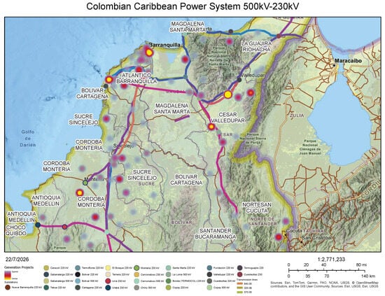
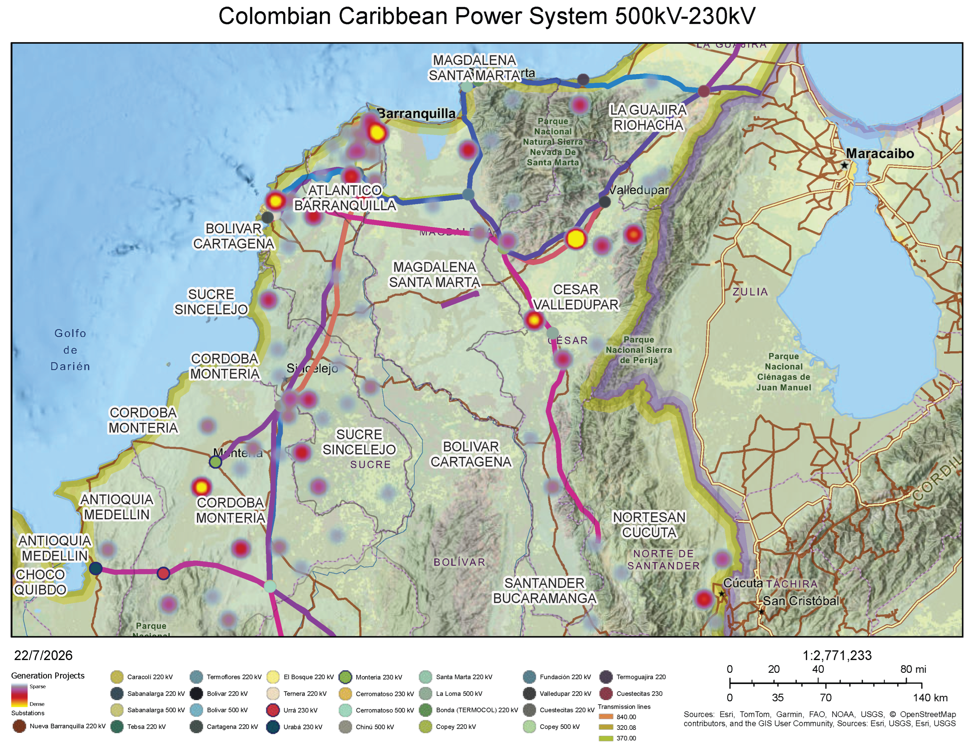
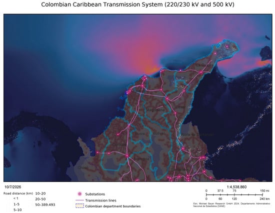
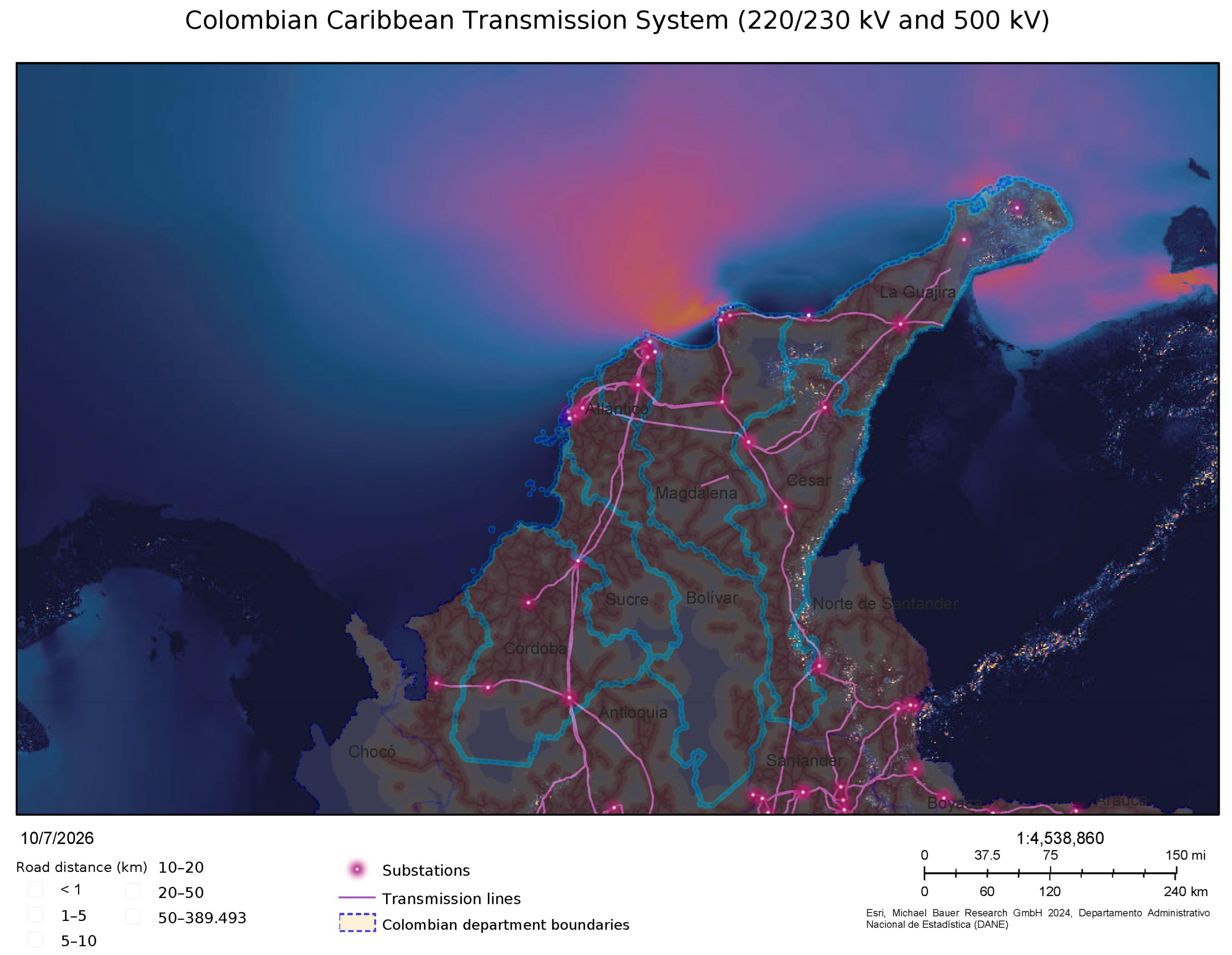
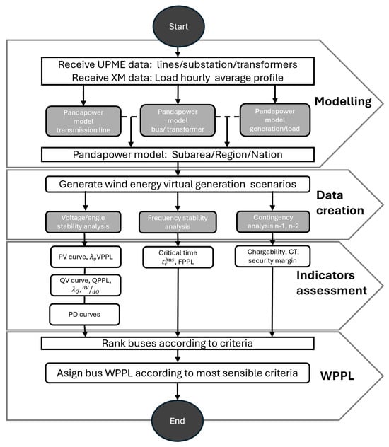
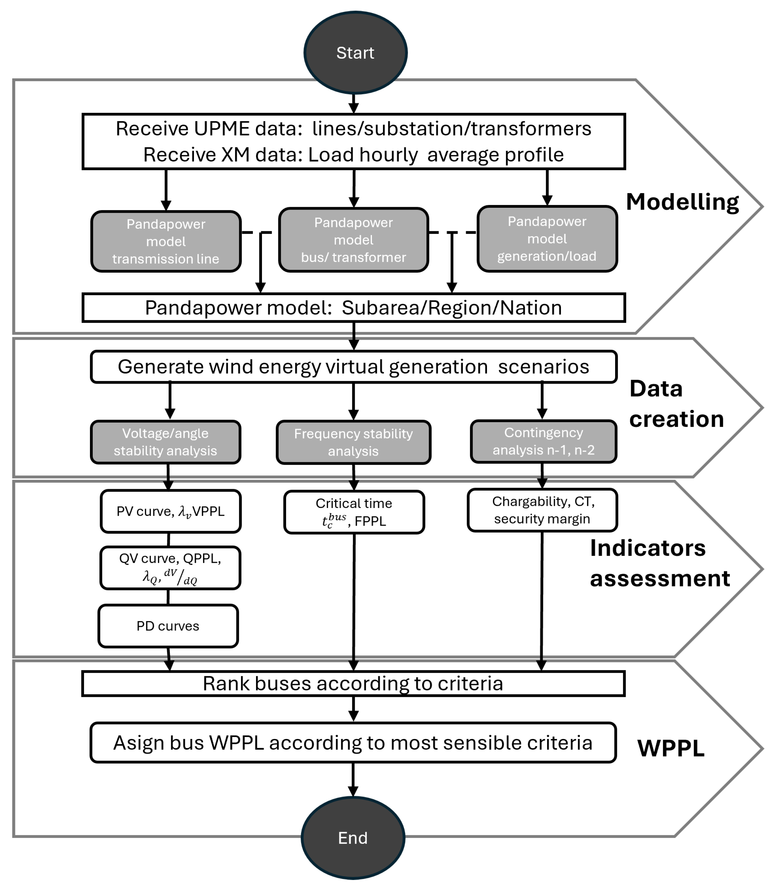
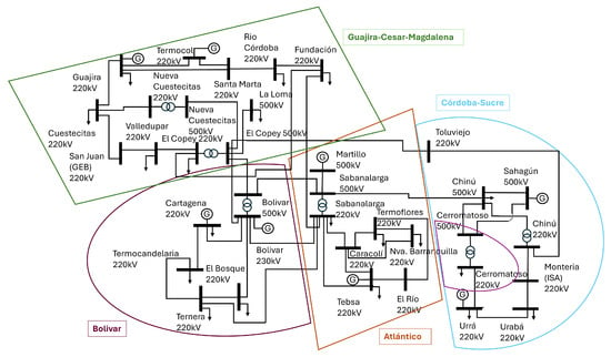
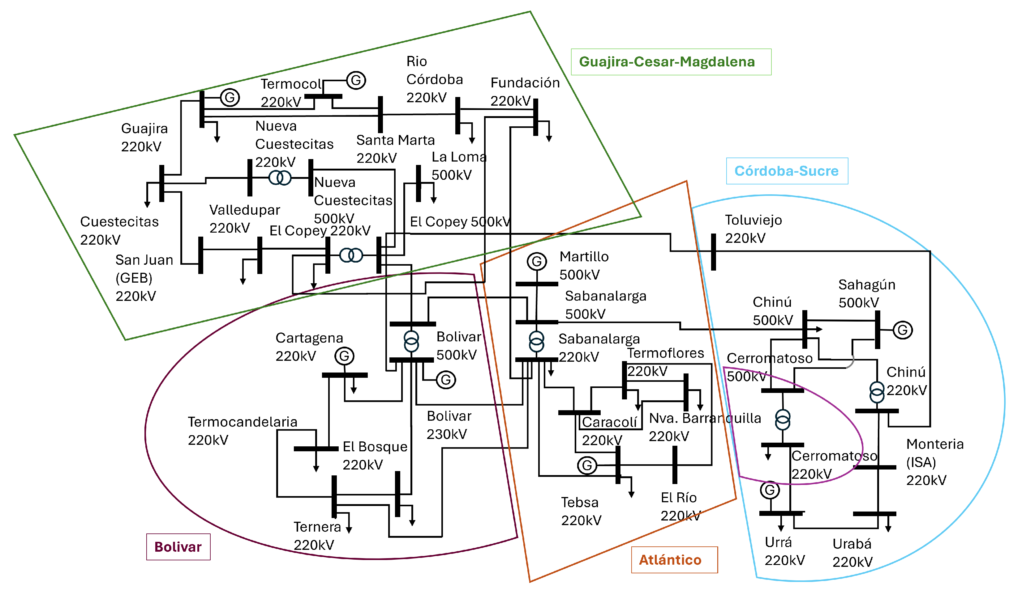
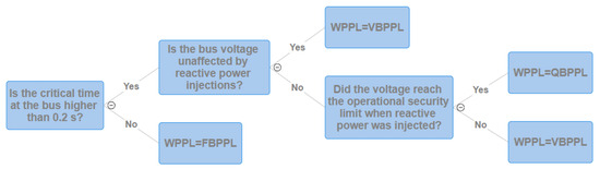
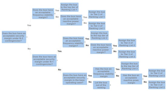
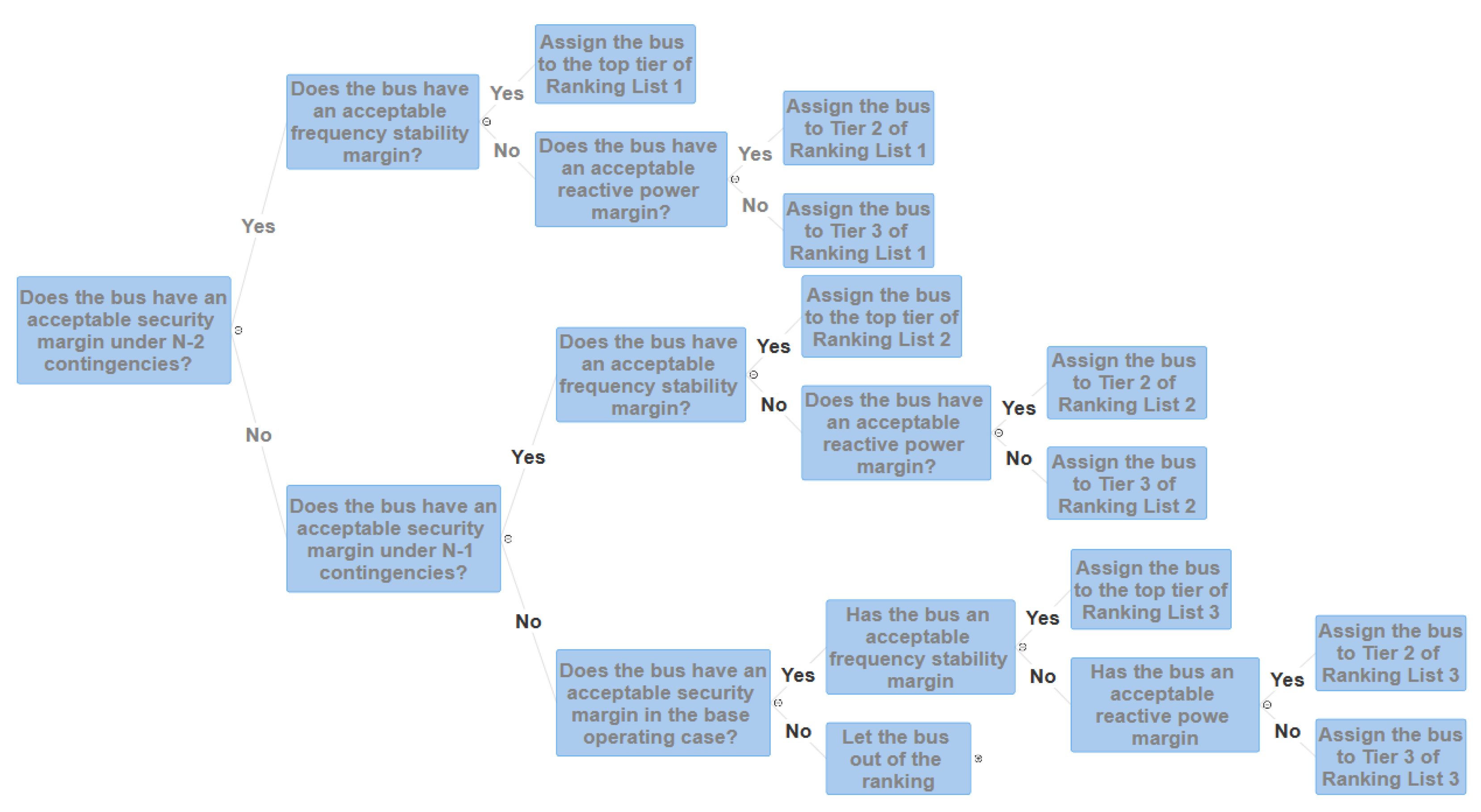
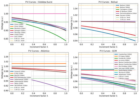
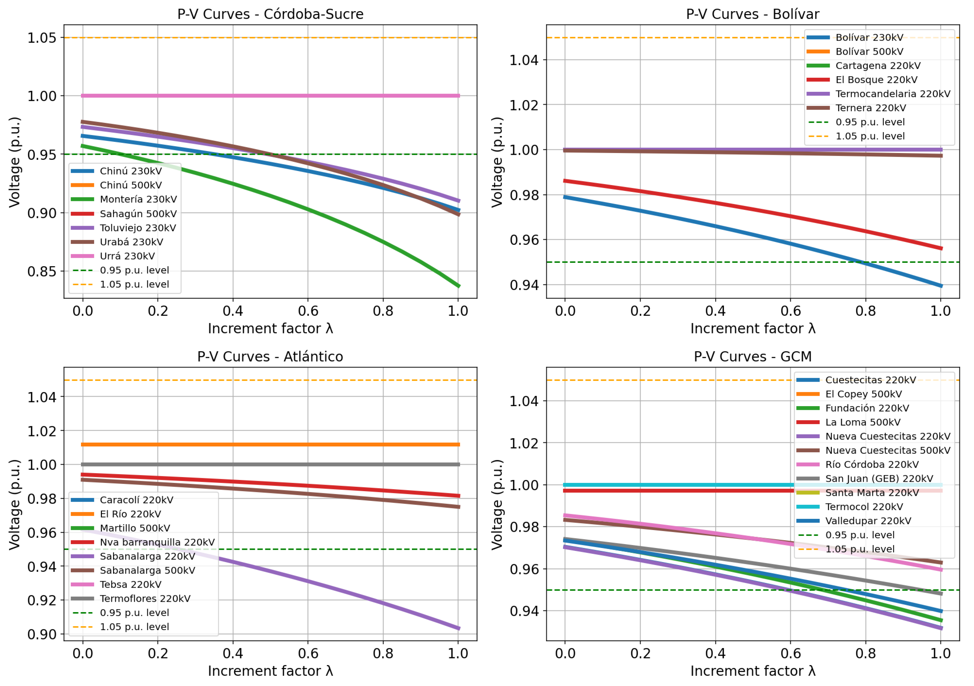
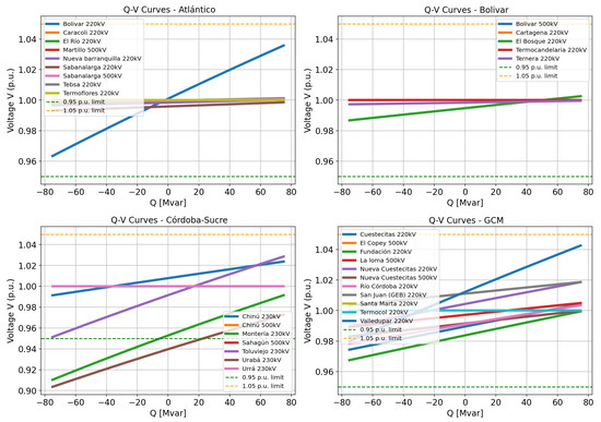
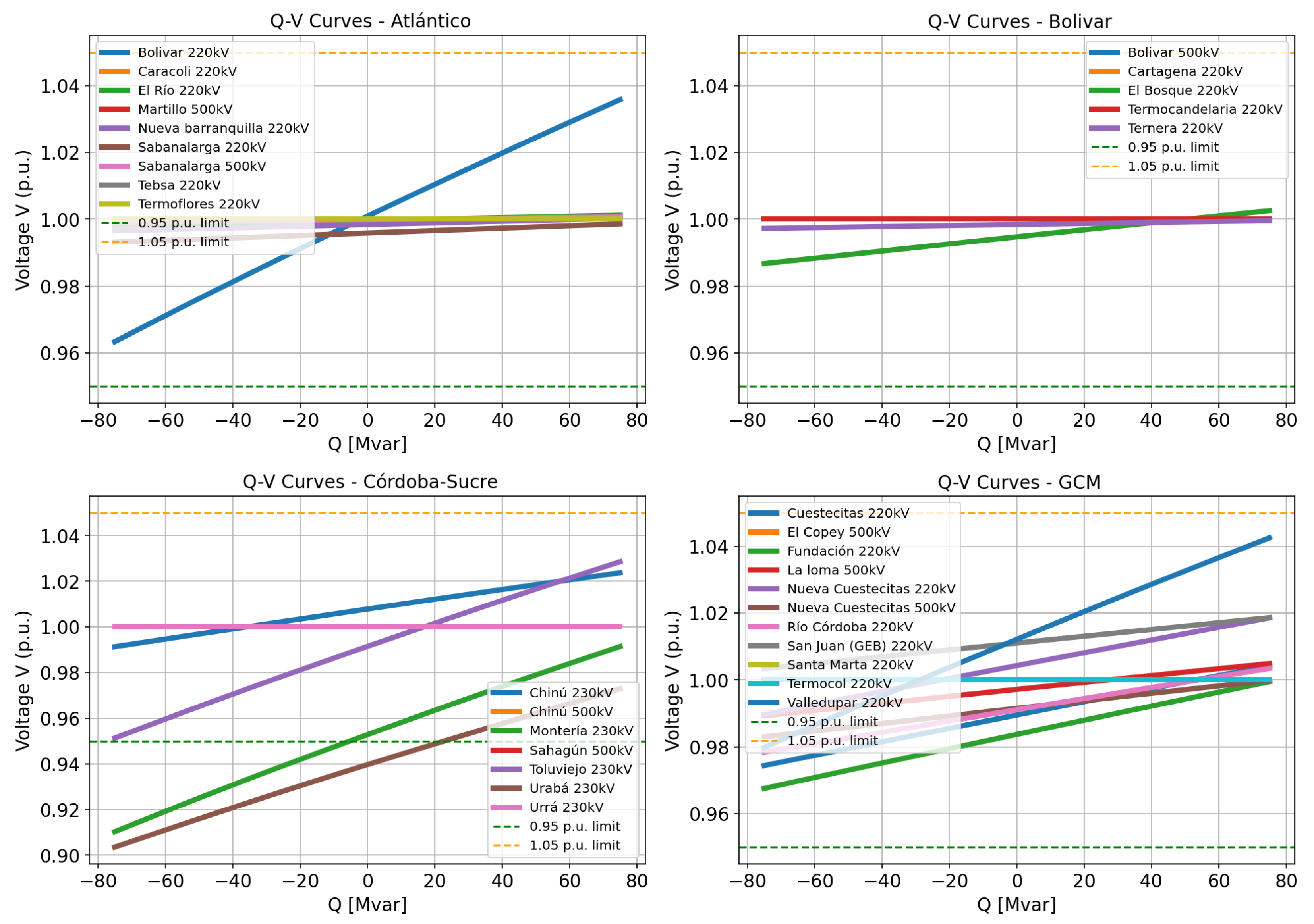
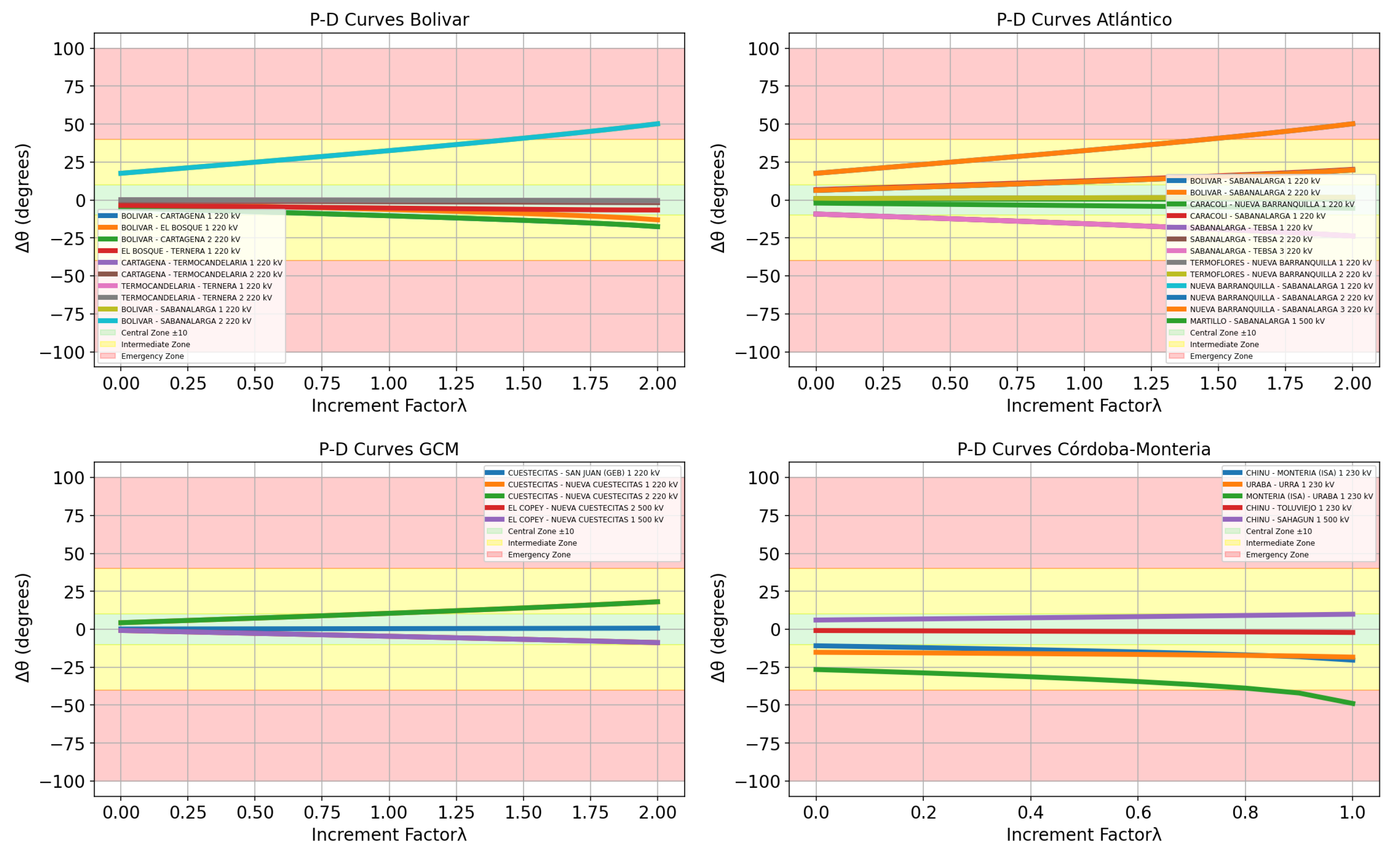
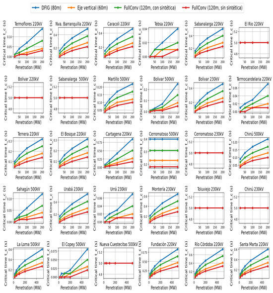
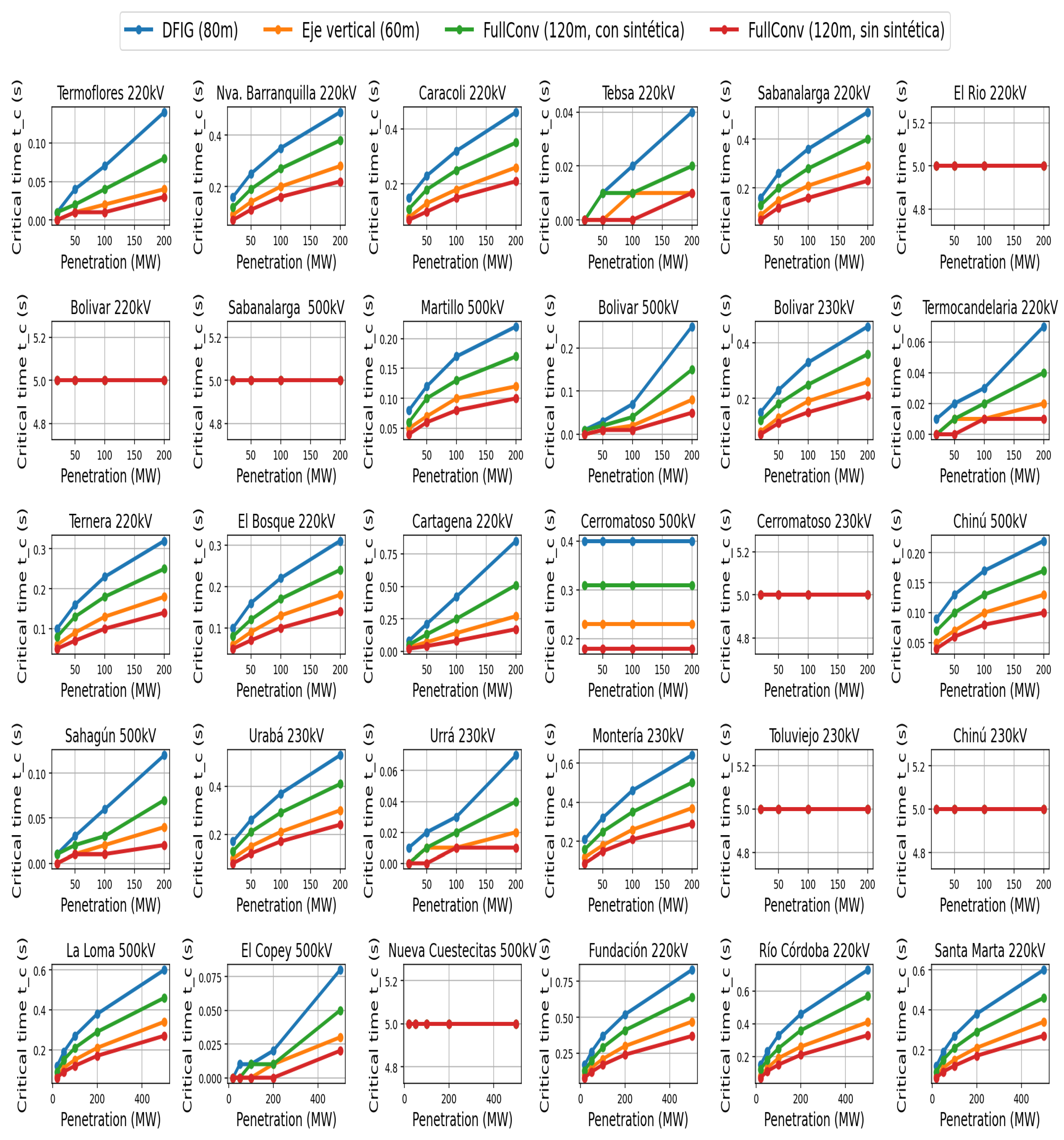
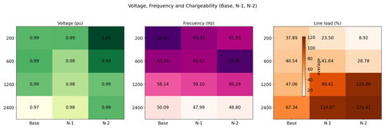
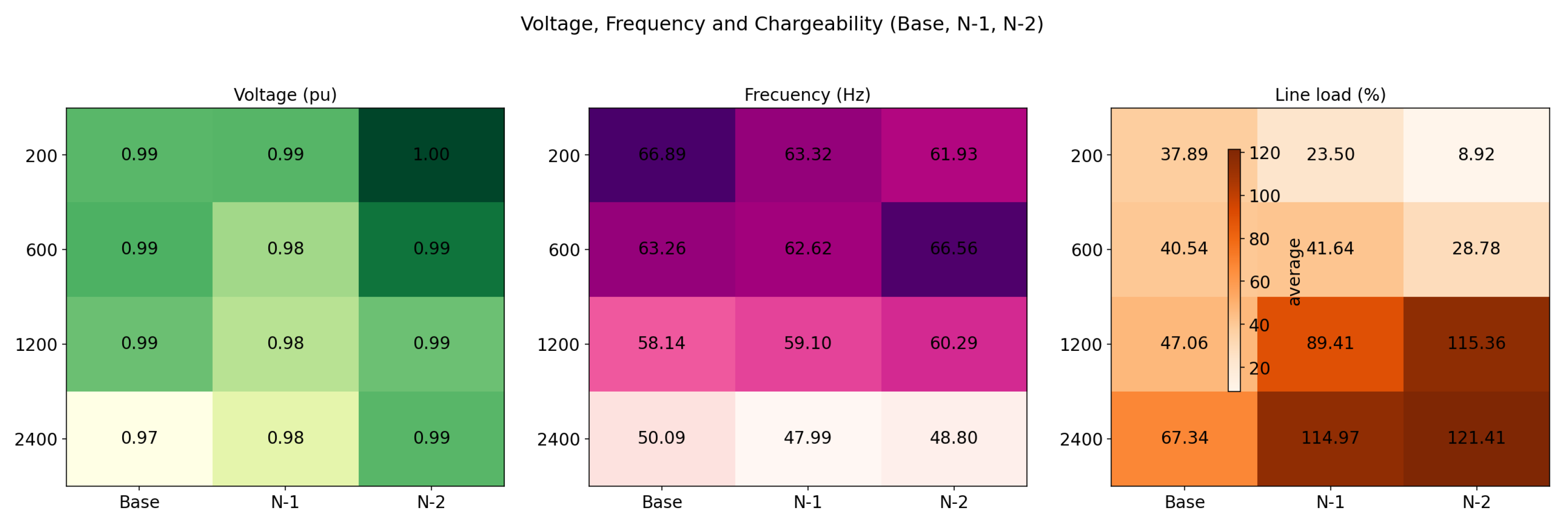
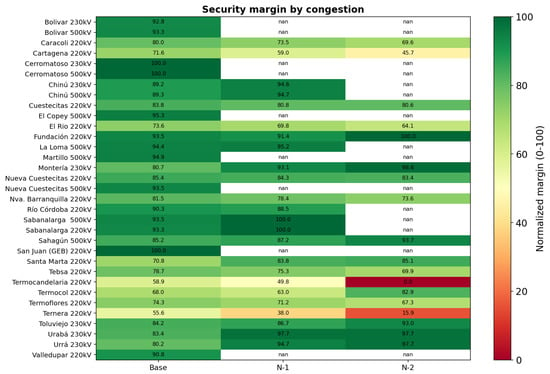
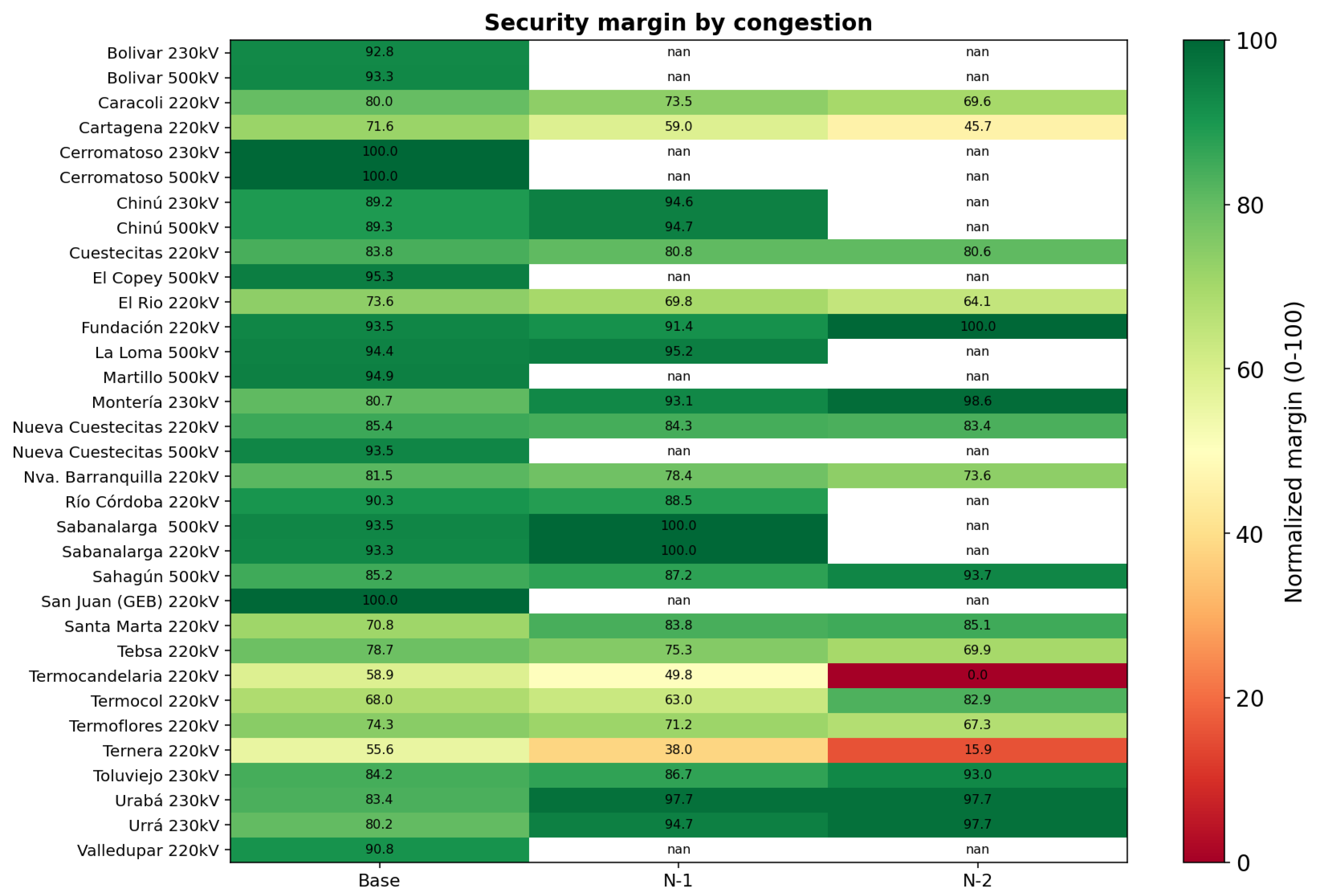
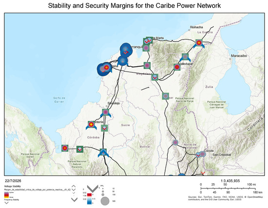
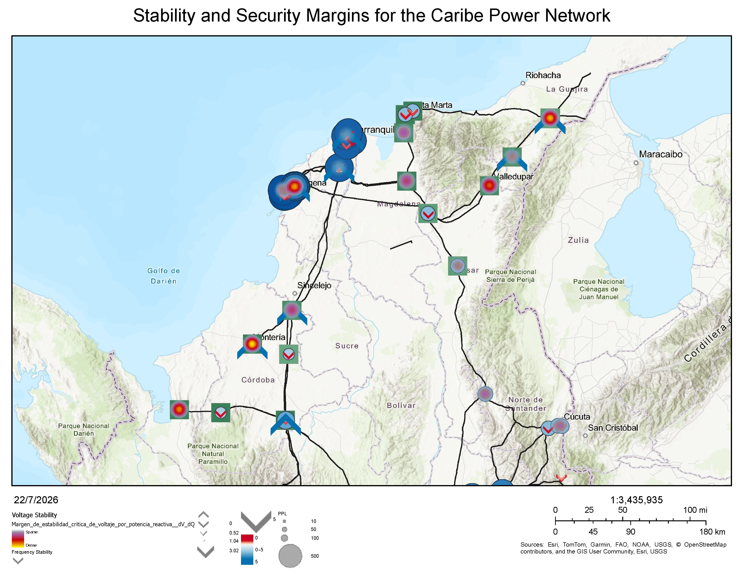
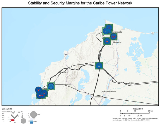
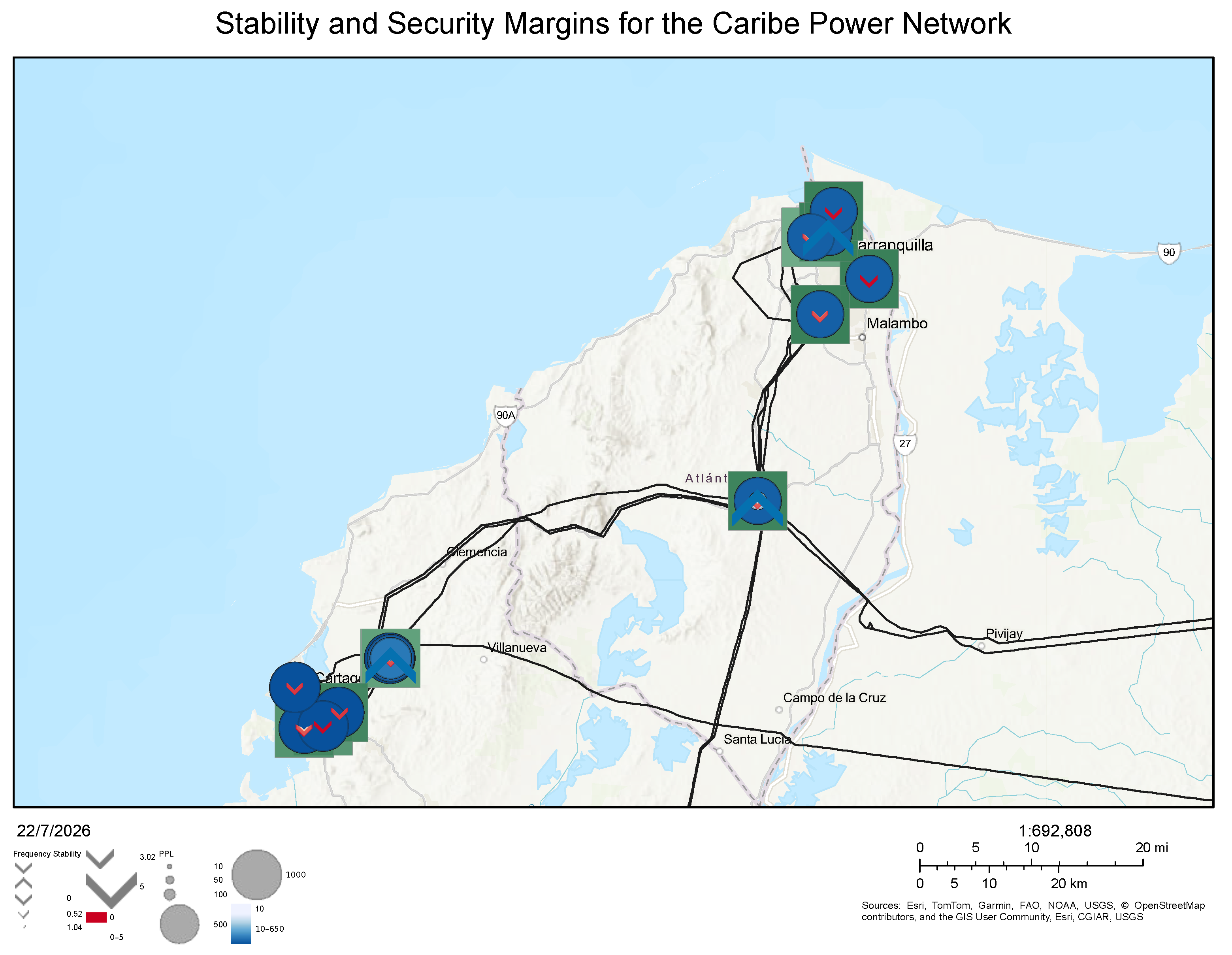

Disclaimer/Publisher’s Note: The statements, opinions and data contained in all publications are solely those of the individual author(s) and contributor(s) and not of MDPI and/or the editor(s). MDPI and/or the editor(s) disclaim responsibility for any injury to people or property resulting from any ideas, methods, instructions or products referred to in the content. |
© 2026 by the authors. Licensee MDPI, Basel, Switzerland. This article is an open access article distributed under the terms and conditions of the Creative Commons Attribution (CC BY) license.