


Abstract
The major challenge in photovoltaic (PV) maximum power point tracking (MPPT) systems is finding a balance between the high performance of artificial intelligence techniques and the interpretability and reliability of physics-based approaches. This paper proposes a new MPPT controller based on a combination of Lagrangian and artificial intelligence techniques. In the proposed method, power maximization is modeled as a Lagrangian system, and the duty cycle is determined by physics equations. An artificial neural network is utilized to adaptively adjust the parameters of inertia and damping in real-time based on an eight-dimensional feature vector. Simulation results for step changes, ramp changes, and partial shading conditions confirm the effectiveness of the approach. The controller has 99.7% tracking efficiency in 18.2 ms, which is superior to P&O (55 ms), INC (45 ms), PSO (28.3 ms), and conventional ANN (22.5 ms). Under partial shading conditions, the controller correctly identifies the global maximum power point. The steady-state ripple is very low (±0.1 W), and the transient energy losses are significantly reduced compared to the benchmark algorithms. The results confirm that the integration of Lagrangian dynamics with adaptive neural tuning provides a systematic and efficient approach for designing reliable PV energy systems, effectively bridging the gap between data-driven and physics-based methods.
1. Introduction
The increasing demand for energy, environmental issues, depletion of natural resources, and geopolitical dynamics are forcing the world to shift toward a new paradigm in power generation, moving from a centralized fossil fuel-based power generation system toward a decentralized renewable energy system. Among the renewable energy systems, solar photovoltaic energy has proved to be one of the most promising due to its modularity, cost reduction, and the potential to harness the sun power directly in the form of electricity [1,2,3]. According to the International Energy Agency, solar photovoltaic energy is one of the most promising emerging energy technologies, with the largest share of the total installed capacity of electricity generators in the world.
Despite their widespread acceptance, PV systems also pose challenges for their large-scale implementation owing to low conversion efficiency and susceptibility to environmental and operational factors. PV modules inherently show nonlinear characteristics in their electrical response that depend on irradiance; temperature; and other factors, such as age and shading effects [2]. Though irradiance affects the PV current and power, temperature affects the PV voltage, and both cause the maximum power point (MPP) to shift along the I-V and P-V curves, respectively. Operation of the PV module at the MPP is essential for efficient power extraction. Any change in load will cause the impedance to change, and as a result, the PV system will be shifted away from the MPP. DC-DC converters such as boost, buck, and SEPIC are commonly used as impedance-matching converters for PV arrays and loads or grid, and their duty cycle is controlled using maximum power point tracking (MPPT) techniques [4].
The conventional MPPT techniques, such as Perturb and Observe (P&O), hill climbing, and Incremental Conductance (INC), are commonly applied owing to their simplicity and low computational complexity [5]. However, the fixed-step-size perturbation of conventional MPPT techniques results in a trade-off between tracking speed and steady-state tracking error, resulting in sustained oscillations around the MPP and sluggish response to dynamic irradiance and load changes [6]. These techniques are also found to be ineffective under partial shading conditions, where the P-V curve has several local maxima, resulting in convergence at non-optimal points and, hence, energy loss [6].
To address the above-mentioned challenges, intelligent and adaptive MPPT techniques have been extensively studied and developed. AI-based techniques, such as fuzzy logic controllers (FLCs), artificial neural networks (ANNs), particle swarm optimization (PSO), and genetic algorithms (GAs), show improved handling of nonlinearities, uncertainties, and PSCs [7,8,9]. Fuzzy logic techniques are promising due to their adaptability and lack of need for mathematical modeling; however, their results depend on the selection of inputs, membership functions, and rule structures. Additionally, many AI techniques are computationally intensive, lack generalization, and are often considered black-box techniques, making it difficult to validate, assess, and analyze the stability of them [10]. Thus, the above challenges underscore the requirement for MPPT schemes that incorporate the flexibility of AI approaches along with the interpretability of physics-based approaches. In this direction, we propose an AI–Lagrangian MPPT scheme. In the proposed scheme, the power-maximization problem for the PV system is formulated based on Lagrangian mechanics [11], which provides an understandable structure for the MPPT problem, whereas the adaptive parameters for the system are determined based on an AI approach.
The controller’s efficacy is validated through simulations using the MATLAB/Simulink R2025a platform, which includes the PV arrays, DC–DC converters, and the controller’s dynamics. Performance is evaluated based on tracking speed, accuracy, and efficiency, using parameters like RMS, RMSE, and overall energy efficiency [12]. In addition, the robustness of the controller is also validated using extreme conditions, which include sudden changes in irradiance, sudden changes in the load, and other complex conditions of partial shading. Thus, this work combines the interpretability of Lagrangian mechanics with the adaptability of AI, resulting in a high-performance, cost-effective, and physics-informed MPPT controller for modern photovoltaic systems.
The organization of the rest of the paper is as follows. In Section 2, the relevant literature on conventional, AI-based, and hybrid MPPT strategies is discussed. The research gap addressed in the current research is also explained. In Section 3, the theoretical background is discussed. This includes the modeling of the photovoltaic system and the development of the Lagrangian-based dynamics for the MPPT. The proposed intelligent control strategy, including the description of the neural network, is discussed in Section 4. Section 5 describes the simulation setup, test scenarios, and performance metrics. Section 6 presents and discusses the simulation results. Finally, the conclusions are drawn in Section 7.
2. Related Works
The MPPT control algorithms used in photovoltaic systems have moved from simple rule-based control to intelligent, hybrid, and physics-based control. This evolution is motivated by the desire for higher accuracy, improved response, and reliable performance under changing conditions. Traditional control strategies, such as Perturb and Observe (P&O) [5], Incremental Conductance (INC) [13], and Constant Voltage (CV) [14], are simple, easy to implement, and hardware-friendly, ensuring reliable performance under steady-state conditions. However, they suffer from limitations such as steady-state oscillations around the maximum power point (MPP) and poor performance under changing conditions [6]. For instance, P&O and INC have efficiencies between 95 and 97%, but they suffer from steady-state oscillations [12], whereas under changing conditions, P&O is known to be trapped by local maxima, leading to reduced accuracy [15]. Other simple control strategies, such as hill climbing and short-circuit current, suffer from limitations related to steady-state conditions, as they assume constant conditions [16].
Various AI-based MPPT techniques, such as artificial neural network (ANN), fuzzy logic controller (FLC), Adaptive Neuro-Fuzzy Inference Systems (ANFISs), and particle swarm optimization (PSO), are also employed to enhance the dynamic response and accuracy of the tracking system [17,18,19,20,21,22,23,24,25]. For example, Ahmed et al. in [17] employed a Supertwisting Sliding-Mode Controller and ANN reference generator, and the results showed that the system achieved 97.8% efficiency, with a response time of 25 ms under changing conditions. Bouselham et al. in [18] used an ANN-based scanning technique, and the results showed that the system achieved 97.64% efficiency, with a response time of 15 ms, even in partial shading conditions.
Demirci et al. [19] further integrated analytical and metaheuristic optimization techniques into the ANN-based MPPT, which achieved 99.98% efficiency under clear-sky conditions and 99.97% under partial-shading conditions. Shadoul et al. [20] and Manna et al. [21] proposed the adaptive fuzzy logic and ANFIS-based MPPT techniques, respectively, which achieved rapid convergence in 24–25 ms with 99.9% accuracy. PSO [9], Ant Colony Optimization [22], Cuckoo Search Optimization [23], Firefly Optimization [24], Whale Optimization [25], Differential Evolution [10], and Grey Wolf Optimization [26] techniques were also proposed for the MPPT of PV arrays under multimodal conditions with high global tracking efficiency and stability. Though the techniques are highly effective for the MPPT of PV arrays, they require large amounts of data for training and computational power, which may restrict their use in PV controllers.
As reported by Farzaneh et al. [27], hybrid MPPT techniques have been developed to integrate the fast response of conventional techniques with the adaptive nature of AI techniques, offering better performance and robustness during varying operating conditions and partial-shading conditions. Some of the techniques include the INC-PSO, P&O-PSO, and fuzzy-based hybrid techniques involving the integration of fuzzy logic control with various forms of metaheuristic techniques, e.g., the fuzzy logic control–PSO, with efficiencies ranging from 97% to 99.5% [27]. Advanced MPPT techniques include the ANN-based fuzzy logic control [20], the hill climbing-based ANFIS [21], and the GWO-based P&O techniques [26], offering faster response and robustness during varying operating conditions. Hybrid MPPT techniques [19,27] have been reported in the literature to achieve efficiencies greater than 99%, with nearly half the convergence time of conventional techniques.
Recently, physics-informed approaches have emerged in various engineering fields by applying Lagrangian and Hamiltonian formulations, which combine energy concepts with intelligent control strategies for stable control systems [11]. The Lagrangian and Hamiltonian formulations were first introduced by classical mechanics, and they have been applied to robotic systems for energy-efficient control strategies, such as trajectory planning [28], and to aerospace systems, such as satellite control systems [29]. In control systems, it has been used to represent the difference between input and output power as a dynamic variable, which inherently provides stability and conserves energy, and the principle of stationary action is used to control systems along paths where energy changes are minimum [11].
Nguyen-Vinh et al. [30] suggested a MAPNN-based MPPT controller, which gave a result of 98.42% efficiency and was more converged than ANN and LSTM approaches under different levels of irradiance.
Mamodiya et al. [31] presented a hybrid approach of physics-informed neural network and reinforcement learning for solar panels’ optimization based on their experimental validation using photovoltaic modules. However, their approach mainly deals with panel orientation and energy yield optimization and not the MPPT duty cycle generation for DC-DC converters.
Energy approaches offer an alternative mechanism-oriented approach to physics-informed neural networks. A Lagrangian-based MPPT technique for a PV system with a buck-boost converter was suggested by Nelatury [32]. This formulation takes the form of a constrained maximum power problem. In a similar way, Phillips-Brenes et al. [33] have developed a sensor-less MPPT approach using a port-Hamiltonian modeling of a PV array connected to a DC-DC boost converter; their results were confirmed using computer simulations and practical experiments.
Control of photovoltaic power electronics using the Euler–Lagrange and port-Hamiltonian approaches is another area that has been researched. Tofighi and Kalantar [34] proposed passivity-based control methods for a stand-alone PV battery system using the port-controlled Hamiltonian and Euler–Lagrange approaches, achieving stability by means of energy shaping and damping. Phillips-Brenes et al. [35] extended the use of the port-Hamiltonian approach for simultaneous MPPT and output voltage control in PV systems with DC–DC buck and boost converters.
Despite the above-mentioned improvements, one crucial methodological difference still stands. The physics-informed neural network (ANN) methods, such as MAPNN [30], introduce physical insights into the learning architecture, while Lagrangian and port-Hamiltonian approaches use the physical structure and energy characteristics of the system to find control strategies [32,33,34,35]. In the presented AI–Lagrangian MPPT framework, the Lagrangian formalism is used to develop an explicit second-order dynamical law for the converter duty cycle control, while an ANN adaptively tunes inertia and damping parameters depending on the current system state. Therefore, the ANN works as an adaptive parameter tuner, and it does not serve as a predictor of the MPP position or as an alternative to the physical model. As far as we know, there is no framework described in the reviewed MPPT literature that incorporates both explicitly derived Lagrangian second-order MPPT dynamics and ANN-tuned parameters of the inertia and damping. The incorporation of the physics-derived control dynamics and ANN parameter adaptation is the principal methodological novelty of the proposed approach.
Based on the stated research gap, the main contributions of the paper are stated below:
- A novel physics-informed Lagrangian MPPT framework that recasts power maximization as a dynamic system, providing interpretability and analytical stability.
- An adaptive neural network for real-time tuning of inertia (J) and damping (D) parameters, ensuring optimal damping (ζ ≈ 0.7) and fast convergence under varying conditions.
- Superior performance validated through simulations, achieving 99.7% tracking efficiency, 18.2 ms settling time, and 100% GMPP detection under partial shading, outperforming P&O, INC, PSO, and ANN methods.
3. Theoretical Foundation and Mathematical Modeling
3.1. Photovoltaic System Modelling
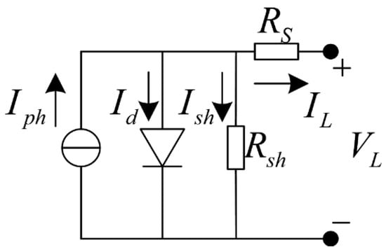
The photovoltaic system is modeled using the five-parameter single-diode model [2], as shown in Figure 1. The current output is given by Equation (1):
where , and () represent the photogenerated current (irradiance-dependent), diode saturation current (temperature-dependent), series resistance (Ω), shunt resistance (Ω), ideality factor, and the thermal voltage, respectively.
Figure 1.
Single-diode equivalent circuit of a photovoltaic cell.
3.2. Dynamics Formulation of the Lagrangian MPPT
The novelty of this work is based on the Lagrangian-based analytical mechanics method, which treats MPPT as a dynamic optimization problem. The Lagrangian function, , is given in Equation (2).
In this equation, the duty cycle value, (), represents the generalized coordinate, whereas the rate of change in the duty cycle value, (), represents the generalized velocity. The kinetic energy and the potential energy are represented as and , respectively. To maximize the power value, , the potential energy is given as . This ensures that the Lagrangian dynamics automatically drive the system toward the duty-cycle values that provide the maximum power extraction. The inertia value, J, behaves as an equivalent mass value. It smooths the motion of the duty cycle toward the maximum power point by controlling the rate of change in the duty-cycle value. To consider the energy loss in the system, the Rayleigh dissipation function is given as . The equation of motion is as follows:
After substitution in the Lagrange equation, the dynamics of the system can be described by the following second-order differential equation, i.e., Equation (4), which describes a virtual mass spring damper system. The gradient of the power is the driving force that tends to move the system toward the MPP:
3.3. Theoretical Analysis of Lagrangian MPPT Dynamics
The Lagrangian MPPT dynamic behavior can be analyzed using the tools of linear system theory in the vicinity of the MPP. The differential equation of the system can be approximated. Numerical methods can be used to analyze the whole nonlinear behavior of the system. The values of the ANN-tuned parameters will generally lead to an effective damping ratio close to the critically damped region (ζ ≈ 0.7). This explains the fast non-oscillatory convergence of the system.
3.3.1. Linear Systems Theory-Based Method
The Lagrangian MPPT linearization assumes small perturbations around the MPP as follows:
- Let , where is the optimal duty cycle at MPP. At the MPP, , the power, is maximal, , and the first derivative satisfies .
- If we expand in a Taylor series around , we get Equation (5):
- At the stationary point, , the first derivative of the power is zero, , and the second derivative, , is negative, indicating a maximum. So, the power function can be approximated by the following function Equation (6), where represents the curvature of the power curve at MPP:
- The power gradient becomes , and the Lagrangian MPPT system equation is given by Equation (7):
The resolution of the differential equation leads to three possible solutions depending on the damping ratio:
- Underdamped (): Oscillatory convergence Equation (8):with corresponding to the natural frequency, and corresponding to the damped frequency.
- Critically damped (): Quickest non-oscillatory convergence Equation (9):
- Overdamped (): Slowest non-oscillatory convergence Equation (10):
The settling time, , to within 2% of final value is around . This linear analysis shows the critical importance of choosing accurate values of J and D for optimal system performance.
3.3.2. Numerical Method
The power function is nonlinear, especially when it is far from the MPP, which makes it very challenging for the Lagrangian equation. Numerical results are preferred for accurate modeling of the nonlinear characteristics of the system [36]. The Lagrangian MPPT system equation, i.e., Equation (4), has a nonlinear term, , on the right-hand side, which is related to the I-V characteristics of the PV system. The analytical results can be achieved for the linearized equation; however, they can be applied only in the neighborhood of the equilibrium point under the assumption of constant J and D parameters. These results can never address the nonlinear characteristics of the system; moreover, numerical instability for the forward Euler method requires that the time step, , should be less than ().
Forward Euler method: When using the forward Euler method [37], the differential equation, i.e., Equation (4), is converted into two first-order equations as follows:
The Euler implementation begins by computing the acceleration in Equation (12). And then we update the speed and the position, respectively, in Equations (13) and (14).
Runge–Kutta (RK4) method: The major drawback of the forward Euler method is that it is only first-order accurate. This forces the method to be conditionally stable, implying that the integration time step, Δt, must be very small to avoid oscillatory or diverging solutions. However, this drawback can be avoided by using the fourth-order Runge–Kutta (RK4) method [37]. This method is based on the following Equation (15):
The state update is then obtained as Equation (16):
where .
Although the RK4 method results in a more accurate numerical solution, it also requires more operations to be performed compared to the forward Euler method. However, for the purpose of a real-time MPPT control system, the simplicity of the algorithm and the reduced latency period are of significant importance. Therefore, the explicit Euler method is used, and the RK4 method could be a future area of improvement.
To handle stiffness in the system, an adaptive time-stepping approach that adjusts Δt dynamically based on local truncation error estimations can be used, i.e., Equation (17):
where represents the user-defined error tolerance, and represents the estimated local truncation error. This adaptive method provides more stable and efficient simulations by reducing the time step, Δt, during sudden changes and increasing Δt during smooth changes in the system.
4. Intelligent Lagrangian MPPT with Adaptive Neural Network Control
While higher-order numerical methods, such as Runge–Kutta (RK4), provide greater precision, this paper uses the explicit Euler method due to its low computational complexity. An adaptive neural network adjusts the J and D parameters, allowing fast and accurate tracking. As shown in the Results section, the algorithm performs very well even with this simple integration approach compared to existing MPPT methods.
4.1. Neural Network-Based Adaptive Parameter Tuning
4.1.1. Adaptive Parameter Tuning Mechanism
In order to adaptively tune the inertia parameter, J, and damping parameter, D, an artificial neural network (ANN) has been integrated into the proposed Lagrangian MPPT algorithm [8,18]. These parameters control the speed of response of the duty cycle to changes in solar irradiance levels while also affecting its smoothness for faster convergence to the MPP. The 8-dimensional features vector is as follows:
The inputs V, I, and P represent the voltage, current, and power at the operating point, respectively. The terms and || (power gradient) indicate the adjustment direction, while and || (duty cycle rate of change) reflect the system dynamics. The input σ(V, I, P) captures variations in V, I, and P, enhancing the ANN’s robustness under fluctuations.
As described in Table 1, the architecture of ANN includes an input layer of eight neurons, three hidden layers of 20, 15, and 10 neurons with ReLU activation for progressive feature extraction and compression, and an output layer of two neurons for J and D with linear activation functions. The total number of parameters is 677.
Table 1.
Neural network architecture details.
The nonlinear relations between performance indicators and control parameters Equation (19) are extracted by the hidden layers, while the output layer is responsible for real-time adaptive tuning.
where corresponds to the activation function, corresponds to the weight matrix, and corresponds to the bias vector. The adaptive tuning of J and D is grounded in the principles of optimal and adaptive control. Since the optimal damping ratio for a second-order system is approximately ζ ≈ 0.7, the optimal damping coefficient is , where represents the curvature of the power-voltage characteristic. Since k varies with environmental conditions, gradient-based adaptation is as follows Equation (20):
The loss function, , is in Equation (21):
This mode of adaptation minimizes the tracking error, as well as the control effort. A smoothing procedure is also included to avoid abrupt changes in the parameters, which could lead to instability. In this procedure, new parameters are computed by using the Equation (22). This smoothing procedure ensures that stability is maintained between changes in control parameters. At the same time, it retains the advantage of ANN tuning, thus making the system robust.
For the physical realizability of the parameters, they are constrained to certain ranges, with J belonging to the range [0.001, 0.05] and D belonging to the range [0.05, 0.3]. The new values are implemented in real time, and the parameter maps for the features are stored for periodic retraining, thus creating a self-improving loop. The ANN regulates the controller’s parameters based on the operating conditions of the system [8]:
- When is large, which means the system is far from the MPP, the ANN reduces the value of J to facilitate faster tracking.
- When the operating conditions are such that is small, the ANN increases the value of J to improve the stability of the system.
- When the duty cycle has large oscillations and is large, the ANN increases the damping parameter, D.
- When is small, the ANN maintains the present value of D.
4.1.2. Neural Network Training and Dataset Construction
ANN training was performed offline based on simulated data using the five-parameter single-diode PV model for a wide range of operational conditions of the PV module, such as irradiance (200–1200 W/m2), temperature (15–65 °C), load resistance (5–50 Ω), and five partial shading cases (0%, 20%, 40%, 60%, and 80%). A total of 75,000 samples were produced using the eight input features presented in Equation (18), whereas the target outputs were the optimal values of inertia and damping parameters, J* and D*, respectively.
The dataset was then randomly split into 70% training, 15% validation, and 15% test data. Input features were normalized using Z-score normalization as described in Equation (23):
where x is the original input feature while and refer to the mean and standard deviation, respectively, computed based on the training data only. The statistics derived from the training set were also used for the validation and test sets to prevent any leakage of information. On the other hand, the target variables J and D were normalized to range between 0 and 1 based on the following:
where and stand for the smallest and largest values of the inertia parameter respectively, whereas and stand for the smallest and largest values of the damping parameter respectively. For this study, = 0.001, = 0.05, = 0.05, and = 0.3. This range was used to scale the data during training, validating, and testing, and later in its online implementation phase.
The artificial neural network architecture is the 8-20-15-10-2 feedforward network as depicted in Table 1. The training was carried out using the Adam optimizer [38], with a learning rate of 0.001, a batch size of 128, and a maximum number of 500 epochs. Early stopping based on the loss during validation was applied to prevent overfitting. The goal of training was to minimize the weighted mean square error between the predicted values of J and D and their optimal scaled values, as well as the L2 regularization term. Loss function is given by
In this equation, N is the number of samples employed in computing the loss for a certain training batch; and represent the estimated scaled inertia and damping, respectively; and and represent the ideal scaled target values of these quantities. The weights assigned to the errors in estimating inertia and damping were taken to be = 0.6 and = 0.4, respectively. The coefficient of L2 regularization was = 10−4, and represents the model’s network weights. For mini-batch training, N is the batch size of 128.
The training and validation losses have been steadily decreasing and have approached the level of 10−4 with almost identical shapes of the two curves, which implies stable convergence and low risk of overfitting. Additional testing on the independent test dataset has proved the trained ANN’s ability to reproduce the optimal parameter mapping in unknown operating conditions.
4.2. Lagrangian-Based MPPT Algorithm
Algorithm 1 illustrates the proposed Lagrangian-based MPPT controller, which integrates dynamic system modeling, neural network–based parameter adaptation, and optimization techniques. A complexity analysis was conducted to verify the feasibility of embedded implementation. The feedforward ANN requires operations per sampling period, while solving the second-order Lagrangian equations has constant complexity, . The total memory requirements are 1 MB approximately, while the latency per sampling interval is less than 50 μs for a sampling frequency of 10 kHz (sampling interval Δts = 100 μs). The integration of the Lagrangian dynamics numerically is done with a time interval of Δt = 10 μs, which is 1/10 of the sampling interval. These results demonstrate that the proposed hybrid controller enables AI-based control with low computational cost, making it suitable for real-time DSP and FPGA implementations.
| Algorithm 1. Lagrangian-Based MPPT with ANN Adaptation. |
| Initialization: Step 1: Measurement and Power Calculation
|
4.3. Engineering Implementation Feasibility
To determine the engineering viability of the designed AI–Lagrangian MPPT controller, the computation and implementation cost was evaluated for typical embedded DSP and FPGA systems. Computation cost is estimated to be about 8200 cycles (54.7 μs) for a 150 MHz TMS320F28335 DSP and 6630 cycles (44.2 μs) for a Xilinx Artix-7 FPGA, which leaves ample computation capacity in the 100 μs MPPT control interval. The memory and computation costs are summarized in Table 2.
Table 2.
Estimated computational and memory requirements of the proposed AI–Lagrangian MPPT controller.
Considerations for practical implementation have also been considered during the control design. The problem of measurement noise is reduced by use of a moving average filter that operates on four sample periods. In order to enhance robustness in the presence of parameter changes and drifts, constraints have been imposed on the adaptive parameters of J ∈ [0.001, 0.05] and D ∈ [0.05, 0.3], while the update is smoothed by α ∈ [0.8, 0.95]. The duty cycle is similarly constrained to its permissible operating range.
Switching and control time scales are chosen in such a way that there is adequate synchronization. Switching frequency for the converter is chosen as 50 kHz and corresponds to = 20 μs, whereas the MPPT control frequency is chosen as 10 kHz, meaning = 100 μs. Therefore, the MPPT is synchronized with switching at a ratio of 5:1. Time constant for numerical integration is chosen as , half of the switching period. This provides adequate temporal resolution for the second-order duty-cycle dynamics.
As a further measure to improve operational reliability, a fallback mode with constant parameters (J = 0.01 and D = 0.1) is provided. If the ANN fails or no new parameter estimates are available, the controller switches to this mode to maintain stable operation. In general, the computational results show that the control algorithm is appropriate for real-time realization in embedded systems (DSP/FPGA).
5. Simulation Framework and Implementation
The simulation model of the proposed AI–Lagrangian MPPT system was developed using MATLAB/Simulink, with Simscape Electrical being utilized to model the nonlinear characteristics of the PV array and the DC-DC boost converter [2,39].
5.1. Simulation Environment and Framework Architecture
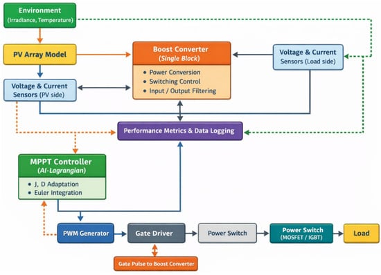
As shown in Figure 2, the simulation framework of the proposed AI–Lagrangian MPPT system can be divided into two layers: one layer for power conversion and one layer for control and intelligence. The power conversion layer of the system consists of the PV array, boost converter, and load, which represents the nonlinear power conversion process of the system [39]. The voltage and current signals of the PV array and boost converter output are utilized as feedback signals for control and evaluation. In the control layer, the proposed Lagrangian-based MPPT formulation described in Section 3 is employed. The dynamic evolution of the duty cycle is described by a second-order equation, i.e., Equation (4), which is numerically integrated with an integration time step of 10 μs, while the sampling period is 100 μs. The parameters J and D are tuned online using the adaptive neural network. The resulting control signal is used to generate a PWM signal using the PWM generator and is finally used to drive the switch using the gate driver interface. In this framework, the distinction between the signal and power flow is made explicit, which is a realistic and implementation-oriented approach to the design and analysis of the control structure.
Figure 2.
Integrated power and control framework of the proposed AI–Lagrangian MPPT-based PV system in MATLAB/Simulink.
5.2. Test Scenarios and Performance Metrics
The performance of the controller was assessed using a set of mathematically described test cases, simulated using MATLAB/Simulink to mimic practical operating situations. Step changes in irradiance levels were simulated using the function Equation (26):
while gradual changes followed a ramp function described by the function Equation (27) [12]:
The occurrence of partial shading, which results in the PV array having several local maxima in the curve, was simulated using several PV array blocks with different inputs for irradiance in Simscape Electrical. This resulted in a cumulative power response described by the function Equation (28) [6]:
Performance metrics were obtained through post-processing of simulation results in MATLAB. Efficiency was calculated by tracking efficiency, which considers sampling effect and steady-state ripple. Dynamic performance was evaluated based on settling time, defined as the time required for the output power to settle within ±2% of its final value after a disturbance. This criterion has been widely applied in MPPT-related research [12]. Further analysis was also conducted to assess the impact of Lagrangian parameters J and D, demonstrating the need for adapting these parameters to achieve convergence and stability.
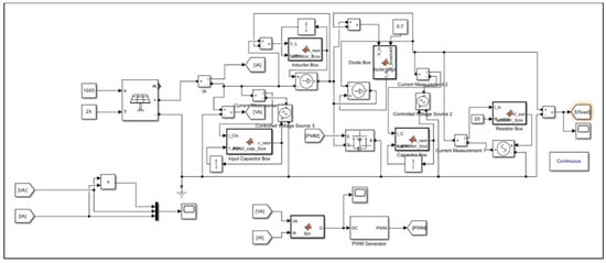
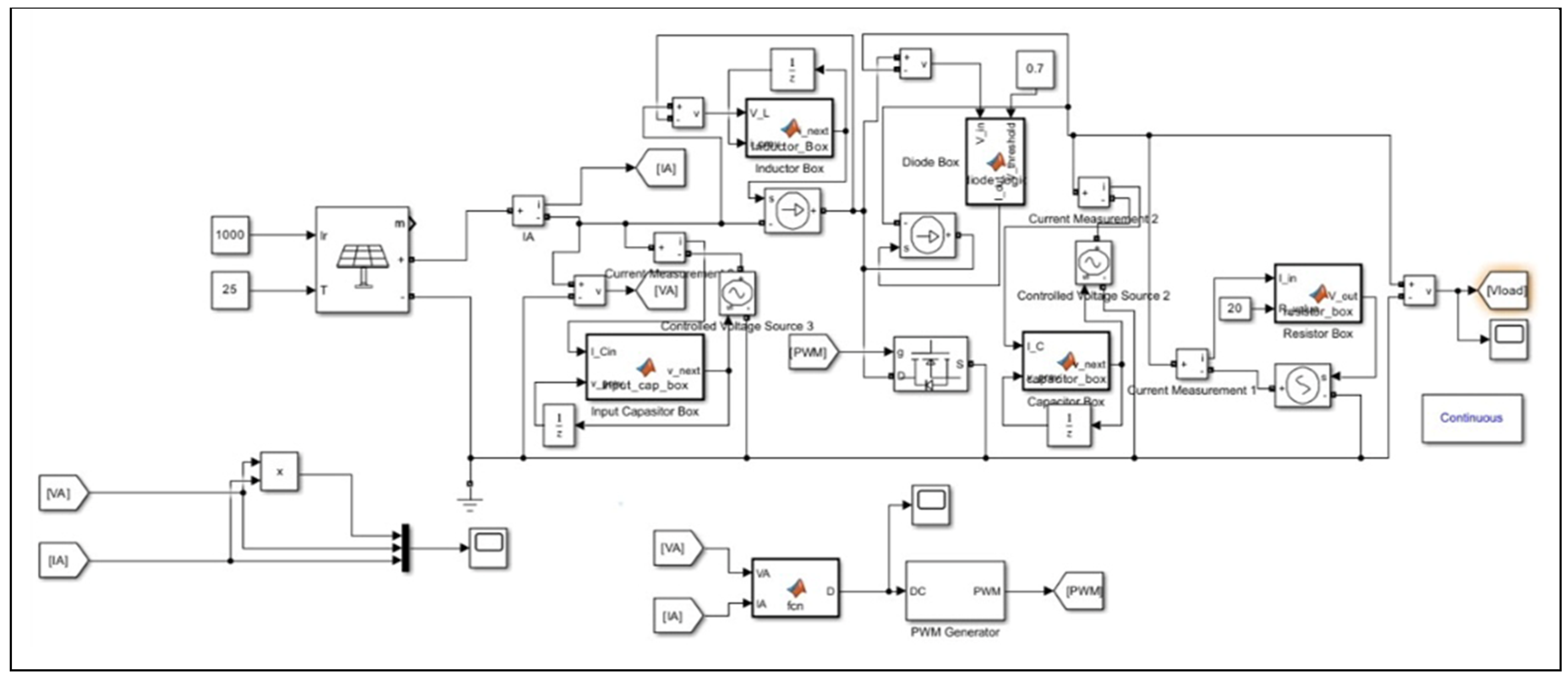
Owing to the nonlinear PV characteristics, switching dynamics of the converter, time-variant environmental conditions, and self-adaptive nature of the AI-based tuning loop, the entire PV-converter-controller system cannot be analyzed using analytical techniques. Numerical simulation becomes the natural choice for analyzing the system [12,30]. Figure 3 shows the entire simulation model of the proposed AI–Lagrangian MPPT PV system, including the PV array, DC-DC boost converter, and Lagrangian MPPT control algorithm that utilizes voltage and current signals from the PV array to compute the duty cycle for the boost converter. Such a simulation model can be utilized to carry out parameter studies, robustness tests, and fair benchmarking of the conventional MPPT algorithms with similar conditions.
Figure 3.
Simulink simulation model of the proposed AI–Lagrangian MPPT-based PV system.
5.3. Benchmark Algorithms Parameter Configuration
For a fair comparison, all the benchmark MPPT techniques were simulated in the same MATLAB/Simulink environment with identical PV system model. The important parameters for each technique were chosen based on the standard configuration in the literature. The parameters were further optimized via simulation trials to achieve consistent performances of the benchmark techniques. Several sets of parameter values for each benchmark algorithm were tested in initial simulation trials before the optimum values were identified. The final values of each parameter used in the benchmark techniques are summarized in Table 3.
Table 3.
Parameter configurations of benchmark MPPT algorithms.
The step sizes for the P&O and INC algorithms were chosen using preliminary testing taking into account the tradeoff between the tracking speed and the steady-state oscillations, as is done in [5,13]. In the case of the PSO, both the population size and number of iterations were chosen by preliminary analysis to get a good compromise between performance and computation costs [9]. The benchmark of the ANN used the same architecture and dataset as the proposed approach in order to make the comparison only valid due to the effect of the proposed adaptation scheme [8]. All benchmark parameters were kept constant in the simulation process and preliminary tuning was done before the final simulation.
6. Results and Discussion
The proposed AI-Lagrange MPPT controller was assessed using simulations in MATLAB/Simulink environment with realistic operating conditions. The controller was implemented with a sampling rate of 10 kHz, whereas the adaptive neural network was utilized to update the Lagrange coefficients J and D using an eight-dimensional measurement vector. The controller was assessed for step change, ramp change, and partial shading cases and was compared with conventional methods such as P&O, INC, PSO, and ANN for the same cases [12]. The performance of the controller was assessed using performance metrics such as tracking efficiency, settling time, and power ripple from the logs for a consistent assessment.
6.1. Comparative Analysis of Dynamic Response to Step Changes in Irradiance
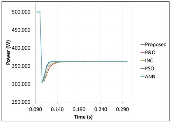
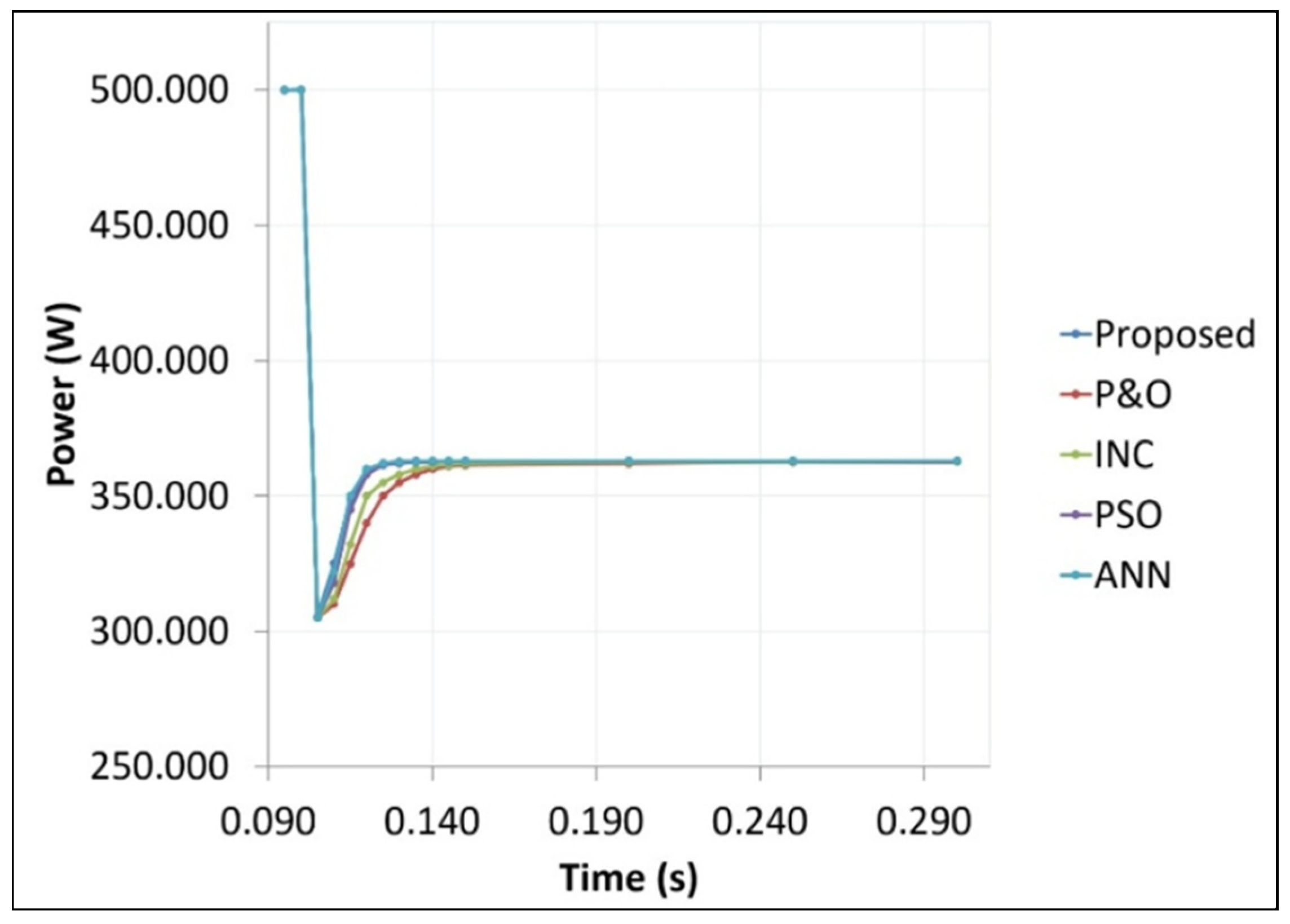
Figure 4 illustrates the comparative dynamic performance of the developed AI–Lagrangian MPPT method and four benchmark methods in the face of an abrupt change in irradiance from 1000 W/m2 to 600 W/m2 at time t = 0.1 s (Table 4). The AI–Lagrangian method demonstrates the shortest settling time of 18.2 ms, thus outperforming the traditional methods of P&O [5], INC [13], PSO [9], and ANN [19], with settling times of 55 ms, 45 ms, 28.3 ms, and 22.5 ms, respectively. The performance of the proposed method is also monotonic and smooth with no overshoot, whereas the performance of the traditional methods of P&O and INC is marred by a high amount of overshoot of 8 W and 5 W, respectively [12]. The performance of PSO and ANN also shows a low amount of overshoot of 3 W and 2 W, respectively. Under steady-state conditions, the performance of the developed method is such that the PV array continues to operate at the MPP with a low amount of power ripple of ±0.1 W, thus outperforming the performance of ANN with a power ripple of ±0.2 W and demonstrating a 50% improvement over the performance of PSO.
Figure 4.
Comparative dynamic response to step change in irradiance showing performance of proposed AI–Lagrangian controller against P&O, INC, PSO, and ANN benchmarks.
Table 4.
Comparative performance metrics following step change in irradiance.
6.2. Global Maximum Power Point Tracking Under Partial Shading
6.2.1. Static Partial Shading with Three PV Modules
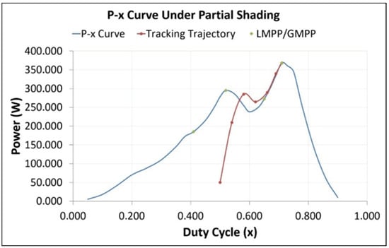
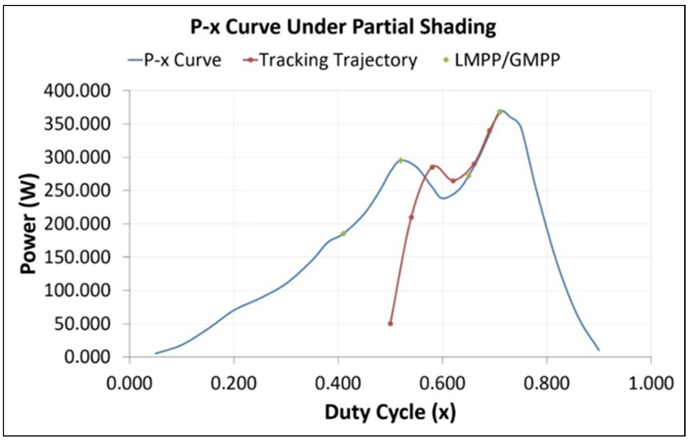
The Power Duty Cycle P(x) curve in Figure 5 is displayed in the case of partial shading. This curve demonstrates the intricate challenge faced during MPPT in traditional systems [6]. Three PV panels experience unequal sunlight irradiation; thus, PV1 experiences 1000 W/m2 of sunlight, PV2 experiences 600 W/m2, and PV3 experiences 400 W/m2. These conditions give rise to multiple peaks at 185 W, duty cycle of 0.41; 295 W, duty cycle of 0.52; and 272 W, duty cycle of 0.65. Maximum power can be achieved at the global maximum power point at 368.5 W with duty cycle of 0.71. It can be observed that the trajectory of the AI–Lagrangian controller follows a global search path, as indicated by its starting point from a low power level of 50.5 W and a duty cycle of 0.50. It can also be observed that the trajectory avoids local maxima and converges to the GMPP, thus validating the effectiveness of deterministic Lagrangian dynamics and adaptive tuning of neural networks [19].
Figure 5.
Multi-modal power–duty-cycle optimization landscape showing global maximum power point search trajectory under partial shading conditions.
6.2.2. Dynamic Partial Shading with Five PV Modules
In order to analyze the response of the controller under the condition of dynamic shading, the irradiance profile was changed from [1000, 800, 600, 400, 300] W/m2 to [800, 500, 300, 700, 400] W/m2 at t = 0.15 s (Table 5).
Table 5.
Performance of the proposed controller under dynamic partial shading.
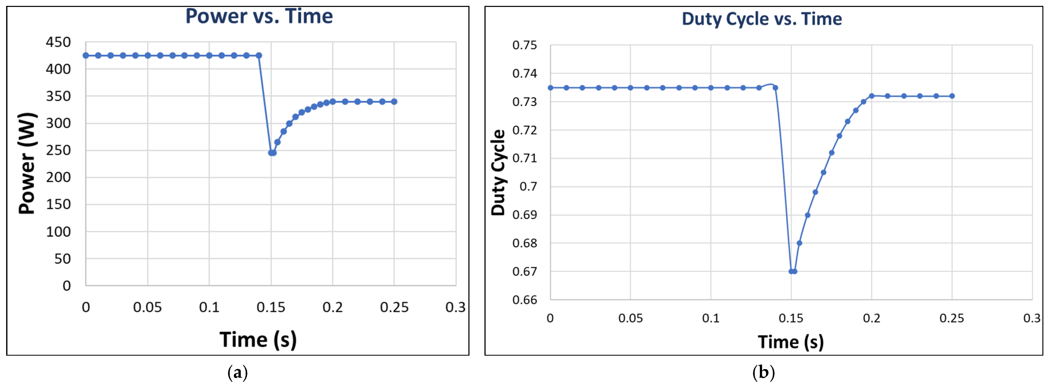
The controller identifies the change in irradiance in 5.2 ms and converges again to the new GMPP with a settling time of 22.8 ms. Transient energy loss due to re-convergence was found to be 0.210 J. In order to conduct an unbiased comparison, all the benchmark methods were run again using the same dynamic-shading scenario. The transient energy losses for P&O, INC, PSO, and ANN were 1.650 J, 1.050 J, 0.430 J, and 0.250 J, corresponding to a decrease of 87%, 80%, 51%, and 16%, respectively. Tracking efficiency in this case was 99.52% and had a steady-state ripple of ±0.15 W. Rate of detection of the GMPP was 100%. It was clearly evident that the controller had succeeded in escaping the local maxima and converging to the new global maximum following the change in the shading pattern. Slightly lower efficiency compared to the static cases can be attributed to the transient losses incurred during the process of re-convergence, but the efficiency still exceeds 99.5%, thus reflecting very high efficiency even in dynamic situations that out-performs the conventional methods and recent ANN based GMPPT techniques [19].
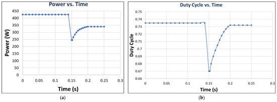
Figure 6 displays the power-tracking behavior and duty-cycle behavior under the dynamic-shading condition. The detection time of the controller for the dynamic-shading condition is 5.2 ms, while the re-convergence time is 22.8 ms. The power is reduced to 245 W before increasing back to 340.0 W, as can be seen from Figure 6a. The transient energy loss is 0.210 J. In order to compare fairly among all benchmark methods, all benchmarks are simulated again under the same condition. All the results are displayed in Table 6. The proposed method gives the lowest transient energy loss (0.210 J), fastest settling time (22.8 ms), smallest steady-state ripples (±0.15 W), and highest tracking efficiency (99.52%). Figure 6b illustrates the duty-cycle behavior: 0.735 before the disturbance, then changed to 0.670 at t = 0.15 s, and finally converged to 0.732. No oscillation observed here implies successful damping behavior. The overall tracking efficiency is 99.52% with the steady-state ripple of ±0.15 W.
Figure 6.
Dynamic response under time-varying partial shading: (a) power-tracking response and (b) duty-cycle evolution.
Table 6.
Comparative performance under dynamic-shading scenario (five PV modules).
6.3. Adaptive Tuning of Lagrangian Parameters: A Signature of Artificial Intelligence
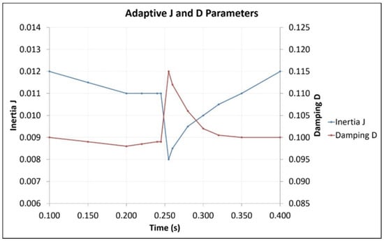
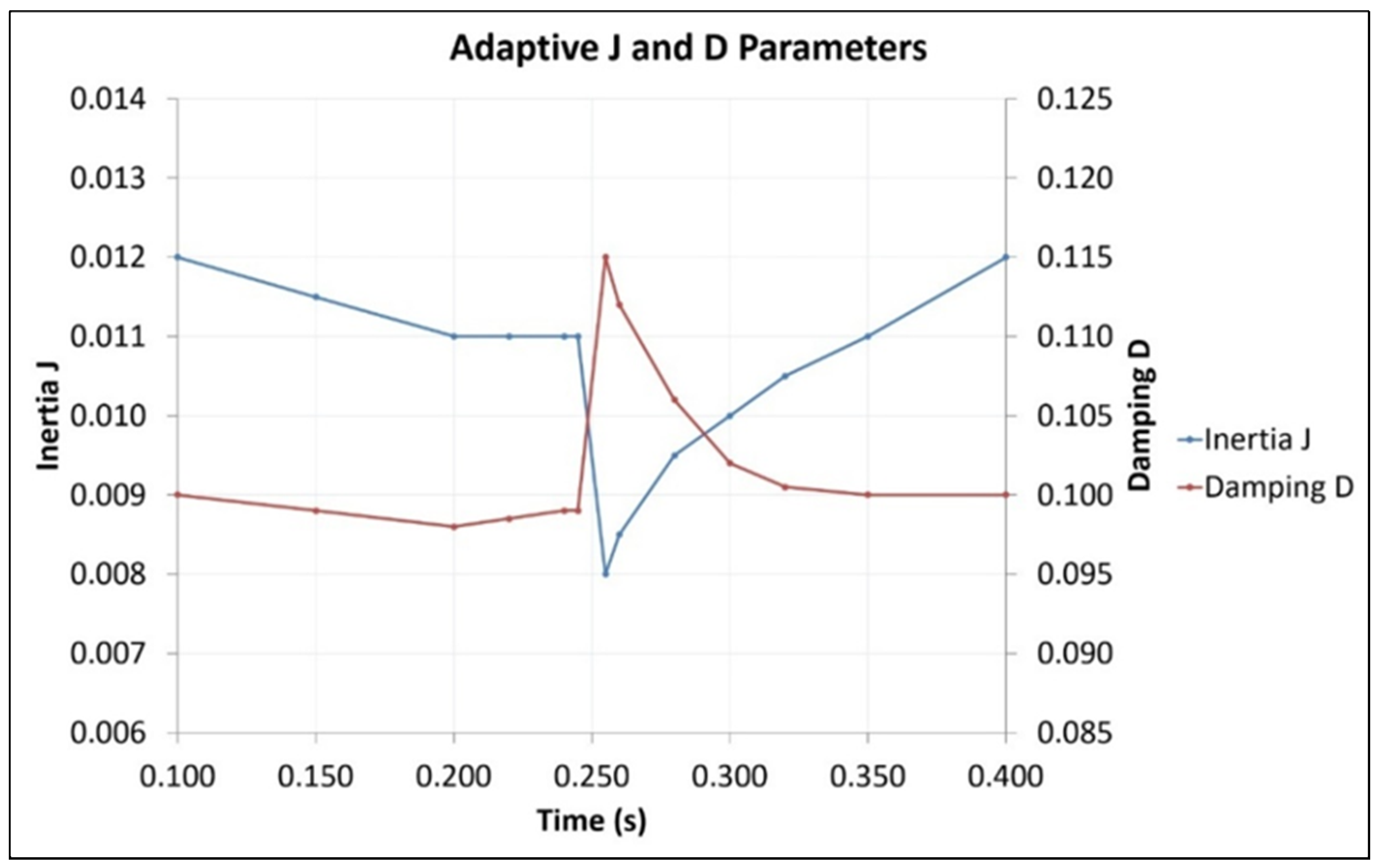
Figure 7 shows how the adaptive tuning process of the proposed AI–Lagrangian MPPT takes place in terms of the dynamic behavior of the inertia (J) and damping (D) values after being modified by the ANN due to variations in the solar irradiance levels. From this figure, it can be seen that during the ramping period (t = 0.1 to 0.25 s), the ANN maintains the two parameter values fairly constant to show the calibrated parameter values for steady-state operations. Nonetheless, right at the moment when the disturbance takes place (t ≈ 0.25 s), the ANN quickly lowers the inertia, J, to be more reactive (from about 0.011 to 0.008). Meanwhile, the ANN raises the damping value, D, from around 0.099 to 0.115 in order to prevent oscillations during the convergence process [36]. The adjustment is anti-correlated and involves a rapid reduction in J, along with a rise in D at the same time. This is a clear indicator of the AI algorithm that is employed in the controller. The dynamic interaction between the inertia and damping coefficients indicates the presence of intelligence in the proposed control scheme. This is because traditional Lagrangian controls, whose parameters remain fixed during the entire process, do not have such dynamics. Normally, the values of the parameters controlled by the proposed neural network-based controller lead to an effective value of the damping coefficient close to critical damping (ζ ≈ 0.7) [11]. Therefore, Figure 7 explains the decision-making algorithm of the AI, thereby making the operation of the controller intelligible.
Figure 7.
Adaptive tuning of inertia (J) and damping (D) parameters during complex irradiance profile, showing anti-correlated adjustment at moment of disturbance.
6.4. Statistical Validation and Energy Efficiency Analysis
To verify the robustness of the proposed controller, a statistical analysis was performed using N = 50 independent simulations for each case, where the weights of the neural network are randomly initialized within ±5% [8]. A summary of the statistical analysis is presented in Table 7.
Table 7.
Statistical performance metrics over 50 simulation runs.
It should be noted that the average ripple power during steady-state condition is found to be 0.81 W, while the ripple power for a typical case is ±0.1 W, as illustrated in Table 7. In order to make clear the difference, the steady-state ripple shown in Table 7 (±0.1 W) indicates the maximum instantaneous power deviation around the operating point [12], and it can be expressed by the following Equation (29):
where P(t) represents instantaneous output power, refers to the mean steady-state power, and is the selected steady-state interval. The mean ripple value listed in Table 7 (0.81 W) is computed statistically over the 50 independent simulations as Equation (30):
Consequently, the disparity arises because of the differing statistical ranges: ±0.1 W is indicative of a representative individual case, while 0.81 W is an average ripple power across the 50 runs. Moreover, the standard deviation is found to be very low, i.e., ±0.06 W.
It also achieves a 100% success rate in GMPP detection under partial shading conditions, thus showing that it can escape local maxima [6]. As far as transient response characteristics are concerned, energy loss, calculated as the integral of power deviation from maximum available power, is found to be as low as 0.148 J, thus showing a 56% improvement over ANN and a significant improvement over conventional P&O method (Table 8) [12].
Table 8.
Energy loss during transient for different MPPT algorithms.
One-way Analysis of Variance (ANOVA) of settling times over all 50 runs shows that p < 0.001, thus rejecting the null hypothesis of equal or comparable performance. Further, post hoc tests using Tukey’s Honestly Significant Difference (HSD) confirm that the proposed method was significantly different from all other algorithms at a confidence level of 95%.
7. Conclusions
This paper proposes a novel hybrid AI–Lagrangian MPPT control strategy that leverages the principles of analytical mechanics to formulate the photovoltaic power maximization problem as a Lagrangian dynamical system, with the duty cycle governed by physics-based equations. The proposed technique utilizes an artificial neural network to adaptively adjust the inertia (J) and damping (D) parameters in real-time, using an eight-dimensional feature vector.
Comprehensive simulations using MATLAB and Simulink for step changes, ramp variations, and partial shading conditions prove the efficacy of the proposed approach. The controller has a tracking efficiency of 99.7%, settling time of 18.2 ms, and minimum steady-state ripple of approximately 0.8 W. A comparative analysis of the proposed approach with P&O, INC, PSO, and ANN techniques demonstrates significant improvement, with a substantial reduction in transient energy loss.
Statistical analysis over 50 simulation runs confirms the robustness of the proposed approach, where the settling time deviation is ±0.43 ms, the tracking efficiency variation is ±0.12%, and a 100% GMPP detection rate is achieved under partial shading conditions.
Adaptive anti-correlation between inertia and damping coefficients is an example of an AI-based adaptation mechanism incorporated into the constrained optimization problem, where convergence is accelerated while maintaining system stability. Moreover, the computational requirements are within acceptable limits for practical implementation, requiring approximately 677 operations per cycle.
In summary, the proposed AI–Lagrangian method closes the performance–explainability gap between data-driven and physics-based approaches. It provides a reliable and efficient MPPT method for PV systems.
Future work will focus on experimental validation and higher-order numerical integration schemes such as the fourth-order Runge–Kutta (RK4) method to further improve numerical accuracy and stability. Moreover, there are several weaknesses of the current study that point out certain directions for further development:
- Optimal conditions for low light operation: The current study was devoted to radiation intensities ranging from 200 to 1200 W/m2. In the future, the operation of the controller in low light (light intensity less than 200 W/m2) will be studied.
- Multi-module series-parallel configuration: The current study is related only to one string of PV panels. In the future, this problem will be solved for several strings of PV modules.
- Hardware-in-the-loop (HIL) testing: In order to fill the gap between simulation and practical implementation, HIL testing will be carried out in order to test the performance of the controller under realistic PV operating conditions, including fast changes in irradiance and temperature, as well as dynamic partial-shading scenarios.
- Outdoor experiment testing: The proposed technique will be tested under outdoor practical conditions in order to test the performance of the technique under realistic solar irradiance and temperature profile and partial shading due to clouds, buildings, and trees.
These modifications will help develop a more comprehensive and reliable AI–Lagrangian MPPT algorithm.
Author Contributions
Conceptualization, M.S.A.M.; Methodology, M.S.A.M., L.F.A.T. and A.Z.; Software, M.S.A.M. and H.I.A.S.; Validation, M.S.A.M. and L.F.A.T.; Formal analysis, L.F.A.T. and A.Z.; Investigation, A.Z.; Resources, M.S.A.M., L.F.A.T. and H.I.A.S.; Data curation, M.S.A.M., L.F.A.T. and H.I.A.S.; Writing—original draft, A.Z.; Visualization, L.F.A.T.; Supervision, A.Z.; Project administration, A.Z. All authors have read and agreed to the published version of the manuscript.
Funding
This research received no external funding.
Data Availability Statement
The original contributions presented in this study are included in the article. Further inquiries can be directed to the corresponding author.
Conflicts of Interest
The authors declare no conflicts of interest.
References
- Ellabban, K.; Abu-Rub, H.; Blaabjerg, F. Renewable energy resources: Current status, future prospects, and their enabling technology. Renew. Sustain. Energy Rev. 2014, 39, 748–764. [Google Scholar] [CrossRef] [Scilit]
- Villalva, M.G.; Gazoli, J.R.; Filho, E.R. Comprehensive approach to modeling and simulation of photovoltaic arrays. IEEE Trans. Power Electron. 2009, 24, 1198–1208. [Google Scholar] [CrossRef] [Scilit]
- Esram, T.; Chapman, P.L. Comparison of photovoltaic array maximum power point tracking techniques. IEEE Trans. Energy Convers. 2007, 22, 439–449. [Google Scholar] [CrossRef] [Scilit]
- Khan, M.; Raza, M.A.; Faheem, M.; Sarang, S.A.; Panhwar, M.; Jumani, T.A. Conventional and artificial intelligence-based maximum power point tracking techniques for efficient solar power generation. Eng. Rep. 2024, 6, e12963. [Google Scholar] [CrossRef] [Scilit]
- Elgendy, M.A.; Zahawi, B.; Atkinson, D.J. Assessment of perturb and observe MPPT algorithm implementation techniques for PV pumping applications. IEEE Trans. Sustain. Energy 2012, 3, 21–33. [Google Scholar] [CrossRef] [Scilit]
- Patel, H.; Agarwal, V. Maximum power point tracking scheme for PV systems operating under partially shaded conditions. IEEE Trans. Ind. Electron. 2008, 55, 1689–1698. [Google Scholar] [CrossRef] [Scilit]
- Boubaker, O. MPPT techniques for photovoltaic systems: A systematic review on current trends and recent advances in artificial intelligence. Discov. Energy 2023, 3, 25. [Google Scholar] [CrossRef] [Scilit]
- Atillah, M.A.; Stitou, H.; Boudaoud, A.; Aqil, M. Performance Analysis of Three MPPT Controls Under Partial Shading: P&O, PSO and ANN. E3S Web Conf. 2023, 469, 00064. [Google Scholar] [CrossRef] [Scilit]
- Singh Chawda, G.; Prakash Mahela, O.; Gupta, N.; Khosravy, M.; Senjyu, T. Incremental conductance-based particle swarm optimization algorithm for global maximum power tracking of solar-PV under nonuniform operating conditions. Appl. Sci. 2020, 10, 4575. [Google Scholar] [CrossRef] [Scilit]
- Tey, K.S.; Mekhilef, S.; Seyedmahmoudian, M.; Horan, B.; Oo, A.T.; Stojcevski, A. Improved differential evolution-based MPPT algorithm using SEPIC for PV systems under partial shading conditions and load variation. IEEE Trans. Ind. Inform. 2018, 14, 4322–4333. [Google Scholar] [CrossRef] [Scilit]
- Goldstein, H.; Poole, C.P.; Safko, J.L. Classical Mechanics, 3rd ed.; Addison-Wesley: Boston, MA, USA, 2002. [Google Scholar]
- Moghassemi, A.; Ebrahimi, S.; Olamaei, J. Maximum power point tracking methods used in photovoltaic systems: A review. Renew. Sustain. Energy Rev. 2020, 124, 109792. [Google Scholar]
- Suwannatrai, P.; Liutanakul, P.; Wipasuramonton, P. Maximum power point tracking by incremental conductance method for photovoltaic systems with phase-shifted full-bridge DC-DC converter. In Proceedings of the 8th ECTI Conference, Khon Kaen, Thailand, 17–19 May 2011; pp. 637–640. [Google Scholar]
- Lasheen, M.; Rahman, A.K.A.; Abdel-Salam, M.; Ookawara, S. Performance enhancement of constant voltage-based MPPT for photovoltaic applications using genetic algorithm. Energy Procedia 2016, 100, 217–222. [Google Scholar] [CrossRef] [Scilit]
- Dhimish, M. Assessing MPPT techniques on hot-spotted and partially shaded photovoltaic modules: A comprehensive review based on experimental data. IEEE Trans. Electron Devices 2019, 66, 1132–1144. [Google Scholar] [CrossRef] [Scilit]
- Eltawil, M.A.; Zhao, Z. MPPT techniques for photovoltaic applications. Renew. Sustain. Energy Rev. 2013, 25, 793–813. [Google Scholar] [CrossRef] [Scilit]
- Ahmed, S.; Muhammad Adil, H.M.; Ahmad, I.; Azeem, M.K.; Huma, Z.; Abbas Khan, S. Supertwisting sliding mode algorithm-based nonlinear MPPT control for a solar PV system with artificial neural networks-based reference generation. Energies 2020, 13, 3695. [Google Scholar] [CrossRef] [Scilit]
- Bouselham, L.; Hajji, M.; Hajji, B.; Bouali, H. A new MPPT-based ANN for photovoltaic system under partial shading conditions. Energy Procedia 2017, 111, 924–933. [Google Scholar] [CrossRef] [Scilit]
- Demirci, A.; Dagal, I.; Tercan, S.M.; Gundogdu, H.; Terkes, M.; Cali, U. Enhanced ANN-based MPPT for photovoltaic systems: Integrating metaheuristic and analytical algorithms for optimal performance under partial shading. IEEE Access 2023, 11, 678–690. [Google Scholar]
- Shadoul, M.; Yousef, H.; Al Abri, R.; Al Hinai, A. Adaptive fuzzy control of three-phase grid-connected inverter. In Proceedings of the 12th International Renewable Engineering Conference (IREC), Amman, Jordan, 14–15 April 2021; IEEE: Piscataway, NJ, USA, 2021; pp. 1–6. [Google Scholar]
- Manna, S.; Singh, D.K.; Akella, A.K.; Abdelaziz, A.Y.; Prasad, M. A novel robust model reference adaptive MPPT controller for photovoltaic systems. Sci. Iran. 2022, 29, 1194–1207. [Google Scholar] [CrossRef] [Scilit]
- Nivetha, V.; Gowri, G.V. Maximum power point tracking of photovoltaic system using ant colony and particle swarm optimization algorithms. In Proceedings of the 2nd International Conference on Electronics and Communication Systems (ICECS), Coimbatore, India, 26–27 February 2015; IEEE: Piscataway, NJ, USA; pp. 948–952.
- Nugraha, D.A.; Lian, K.L.; Suwarno. A novel MPPT method based on cuckoo search algorithm and golden section search algorithm for partially shaded PV systems. Can. J. Electr. Comput. Eng. 2019, 42, 173–182. [Google Scholar] [CrossRef] [Scilit]
- Zhang, M.; Chen, Z.; Wei, L. An immune firefly algorithm for tracking the maximum power point of PV arrays under partial shading conditions. Energies 2019, 12, 3083. [Google Scholar] [CrossRef] [Scilit]
- Cherukuri, S.; Rayapudi, S. A novel global MPP tracking of photovoltaic systems based on whale optimization algorithm. Int. J. Renew. Energy Dev. 2016, 5, 225. [Google Scholar] [CrossRef] [Scilit]
- Guo, K.; Cui, L.; Mao, M.; Zhou, L.; Zhang, Q. An improved gray wolf optimizer MPPT algorithm for PV systems with BFBIC converter under partial shading. IEEE Access 2020, 8, 103476–103490. [Google Scholar] [CrossRef] [Scilit]
- Farzaneh, J. A hybrid modified FA-ANFIS-P&O approach for MPPT in photovoltaic systems under partial shading conditions. Int. J. Electron. 2019, 107, 703–718. [Google Scholar]
- Siciliano, B.; Khatib, O. (Eds.) Springer Handbook of Robotics, 2nd ed.; Springer: Berlin/Heidelberg, Germany, 2016. [Google Scholar]
- Wie, B. Space Vehicle Dynamics and Control, 2nd ed.; AIAA Education Series: Reston, VA, USA, 2008. [Google Scholar]
- Nguyen-Vinh, K.; Rangaraju, S.; Jasinski, M. Mod Tanh-Activated Physical Neural Network MPPT Control Algorithm for Varying Irradiance Conditions. Energy Sci. Eng. 2025, 13, 2606–2619. [Google Scholar] [CrossRef] [Scilit]
- Mamodiya, U.; Kishor, I.; Almaiah, M.A.; Hamdi, M.; Shehab, R.; Alkhdour, T. Numerical modeling and neural network optimization for advanced solar panel efficiency. Sci. Rep. 2025, 15, 23492. [Google Scholar] [CrossRef] [Scilit] [PubMed]
- Nelatury, S.R. A maximum power point algorithm using the Lagrange method. J. Power Sources 2013, 234, 119–128. [Google Scholar] [CrossRef] [Scilit]
- Phillips-Brenes, H.; Pereira-Arroyo, R.; Rímolo-Donadío, R.; Muñoz-Arias, M. Current-sensorless control strategy for the MPPT of a PV cell: An energy-based approach. Int. J. Photoenergy 2022, 2022, 1747533. [Google Scholar] [CrossRef] [Scilit]
- Tofighi, A.; Kalantar, M. Interconnection and damping assignment and Euler-Lagrange passivity-based control of photovoltaic/battery hybrid power source for stand-alone applications. J. Zhejiang Univ. Sci. C 2011, 12, 774–786. [Google Scholar] [CrossRef] [Scilit]
- Phillips-Brenes, H.; Muñoz-Arias, M.; Pereira-Arroyo, R.; Esquivel-Sancho, L.M.; Rimolo-Donadio, R. Passivity-based control approach for photovoltaic DC-DC conversion and output voltage regulation. IEEE Trans. Control Syst. Technol. 2025, 33, 479–492. [Google Scholar] [CrossRef] [Scilit]
- Khalil, H.K. Nonlinear Control, 3rd ed.; Pearson: London, UK, 2015. [Google Scholar]
- Butcher, J.C. Numerical Methods for Ordinary Differential Equations, 3rd ed.; Wiley: Hoboken, NJ, USA, 2016. [Google Scholar]
- Al-Husban, Y.; Al Smadi, T.; Laha, S.R.; Al Smadi, K. Photovoltaic stand-alone systems using an artificial neural network-based intelligent control system. Tikrit J. Eng. Sci. 2025, 32, 1–16. [Google Scholar] [CrossRef] [Scilit]
- MathWorks. Solar PV System with Maximum Power Point Tracking Using Extremum Seeking Control. MATLAB & Simulink Documentation. 2025. Available online: https://www.mathworks.com/help/slcontrol/ug/mppt-in-solar-pv-using-esc.html (accessed on 16 September 2026).

Disclaimer/Publisher’s Note: The statements, opinions and data contained in all publications are solely those of the individual author(s) and contributor(s) and not of MDPI and/or the editor(s). MDPI and/or the editor(s) disclaim responsibility for any injury to people or property resulting from any ideas, methods, instructions or products referred to in the content. |
© 2026 by the authors. Licensee MDPI, Basel, Switzerland. This article is an open access article distributed under the terms and conditions of the Creative Commons Attribution (CC BY) license.