Probabilistic Power Forecasting for Photovoltaic Plant Clusters Using VMD-GCN-Informer

Abstract

Existing photovoltaic (PV) power forecasting methods face challenges in simultaneously capturing multi-scale temporal characteristics, spatial dependencies among PV plants, long-term temporal correlations, and output uncertainty. To address these issues, this paper proposes a spatiotemporal probabilistic forecasting framework for PV plant clusters that integrates Variational Mode Decomposition (VMD), Graph Convolutional Networks (GCN), Informer, and Quantile Regression (QR). VMD decomposes non-stationary PV power series into components with different frequency characteristics, while GCN captures spatial dependencies among PV plants. Informer efficiently models long-term temporal dependencies, and QR generates probabilistic forecasts to quantify output uncertainty. The proposed VMD-GCN-Informer-QR model is evaluated using data from the Australian DKASC PV system. At the 5-min forecasting horizon, the proposed model obtains an MAE of 42.834 kW and the lowest RMSE of 72.182 kW. For probabilistic forecasting, the proposed model achieves a PICP of 89.682%, with an MPIW of 201.818 kW. Multi-step forecasting further shows that the proposed model outperforms Persistence from 15 to 60 min, with its relative advantage increasing as the forecasting horizon extends. Seasonal analysis also confirms the adaptability of the proposed model under different seasonal conditions. These results demonstrate the effectiveness of the proposed framework in limiting large forecasting errors, quantifying forecasting uncertainty, and maintaining robust performance over extended forecasting horizons.

1. Introduction

With the rapid advancement of new energy generation technologies, photovoltaic (PV) power has seen a continuous expansion in its installed capacity within power systems, owing to its advantages such as cleanliness, low carbon emissions, and renewability. Against the backdrop of large-scale integration of distributed photovoltaics, multiple PV stations are increasingly operating in clusters, gradually becoming a vital component of distribution networks and modern power systems. However, PV power output is influenced by various meteorological factors, including solar irradiance, ambient temperature, and cloud cover variations, exhibiting significant characteristics of randomness, volatility, and intermittency. The uncertainty is further superimposed and amplified at the cluster level, posing severe challenges to the safe and stable operation of the grid, power balance control, and dispatch decision-making. Accurate Photovoltaic Power Forecasting (PVPF) plays a crucial role in optimizing grid operations, minimizing energy waste, enhancing solar energy efficiency, and improving the profitability of PV power plants [1]. Therefore, to effectively address these issues, it is imperative to develop high-precision forecasting methods for PV clusters. In particular, probabilistic forecasting approaches, which are specifically designed to characterize and quantify such uncertainty, hold profound theoretical significance and practical engineering value.

1.1. Literature Review

Existing PV power forecasting methods primarily include physical mechanism-based modeling, statistical analysis-based methods, and data-driven intelligent forecasting approaches. Physical models rely on complex meteorological parameters and system configurations, such as tilt angles and conversion efficiency, to directly calculate theoretical output [2,3]. These models involve high construction costs and exhibit poor adaptability. Statistical forecasting methods focus on mining time-series patterns from historical power data to establish mathematical models for prediction. Typical techniques include the Autoregressive Moving Average (ARMA) model, Autoregressive Integrated Moving Average (ARIMA) model, Grey Prediction Model, and Markov Chains [4,5,6]. However, these methods demonstrate limited capability in handling the strong nonlinearity and non-stationarity inherent in PV power sequences.

With the advancement of artificial intelligence, neural network models have been gradually introduced into the field of PV power forecasting. Typical approaches include Back-Propagation neural networks (BP), Radial Basis Function neural networks (RBF), Artificial Neural Networks (ANN), and Support Vector Machines (SVM) [7,8,9]. In recent years, deep learning techniques such as Recurrent Neural Networks (RNN) [10], Long Short-Term Memory (LSTM), and Gated Recurrent Units (GRU) [11] have been widely applied to PV power forecasting. Compared with traditional feed-forward neural networks, these deep learning models can capture complex time-series relationships within the data, making them suitable for nonlinear and dynamic load data.

Recent forecasting methods have further introduced hybrid CNN-LSTM structures [12], which combine convolutional layers for local feature extraction with LSTM for capturing temporal dependencies, thereby achieving precise modeling of complex time series. Wang et al. [13] use a hybrid forecasting framework that integrates LSTM-RNN with temporal correlation correction, leveraging the coupling relationship between the periodicity and randomness of PV output. This approach captures nonlinear fluctuation characteristics and refines preliminary results based on annual cycle patterns and neighborhood similarity, enhancing short-term forecasting performance. While neural network models demonstrate significant advantages in nonlinear modeling, they still suffer from diminished accuracy in long-term time-series forecasting.

In addition, the Transformer model captures global dependencies in time series through the self-attention mechanism, showing excellent performance in long-sequence forecasting tasks. Some studies have introduced the Transformer structure into PV power forecasting, effectively improving prediction accuracy. However, the computational complexity of the standard Transformer increases quadratically when modeling long sequences, making it difficult to meet the requirements of engineering applications. To address this, some researchers have adopted the Informer model [14]. By using a ProbSparse self-attention mechanism and a distilling structure, Informer significantly reduces computational complexity while maintaining high accuracy. This model has achieved good results in fields such as power load and wind power forecasting. Despite its strengths in long-term forecasting, the application of Informer in medium-term forecasting remains relatively limited, as it struggles to effectively capture the more complex short-term fluctuations and seasonal variations inherent in medium-term predictions.

To achieve better performance in PV power forecasting, researchers have employed various hybrid approaches. Kushwaha and Pindoriya [15] applied wavelet decomposition to split the original sequence into sub-sequences of different frequencies. They then established linear Seasonal ARIMA (SARIMA) models and nonlinear Random Vector Functional Link (RVFL) neural networks for each sub-sequence. The final forecast was obtained by summing and reconstructing the predictions of all sub-sequences, achieving superior accuracy compared with single models or other hybrid approaches, particularly under highly volatile weather conditions. Niu et al. [16] utilized Complementary Ensemble Empirical Mode Decomposition (CEEMD) to decompose non-stationary power sequences into multiple Intrinsic Mode Functions (IMFs), reducing sequence volatility. They optimized the weights and thresholds of a Back-Propagation Neural Network (BPNN) using the Dynamic Inertia Factor Particle Swarm Optimization (DIFPSO) algorithm, effectively mitigating the model’s tendency to get trapped in local optima and significantly improving prediction accuracy under various weather types. Tang et al. [17] proposed a hybrid model for short-term forecasting based on feature construction and an improved Transformer. They applied the FOX algorithm to optimize Complete Ensemble Empirical Mode Decomposition with Adaptive Noise (CEEMDAN) for modal decomposition and introduced a frequency-enhanced channel attention mechanism into the iTransformer architecture to emphasize frequency-domain information within multivariate time series. This approach notably enhanced both prediction accuracy and model generalization. Li et al. [18] developed a combined model integrating CNN, Bidirectional Long Short-Term Memory (BiLSTM) networks, and an Attention Mechanism (AM), with global hyperparameter optimization performed using a Feature Optimization Algorithm (CFOA). The model first uses CNN to extract spatial features and BiLSTM to capture hidden temporal dependencies. A self-attention mechanism is then employed to automatically assign feature weights and model long-term dependencies, resulting in an optimized hybrid forecasting framework. Tian et al. [19] proposed a SHAP-NMTCN-BiGRU-based model for short-term forecasting, incorporating nonlinear prediction and secondary error correction. This method first classifies weather types using the MCClear model and applies Random Forest to enhance features of abrupt weather subsets. SHAP values are employed to optimize weighting across models and feature dimensions, while Neural Architecture Search (NAS) automatically tunes the hybrid network structure. Finally, the initial prediction error is calculated, and a Transformer model is introduced for linear error prediction and secondary correction of power values. However, most existing studies focus on individual PV power stations and primarily model temporal features, often neglecting the spatial correlations within PV clusters. As a result, fully characterizing the power evolution patterns of PV clusters remains challenging.

In practical operation, the substations within a PV power plant cluster exhibit significant spatial correlations in terms of geographical location, meteorological conditions, and operating status. This spatial dependency has an important impact on the overall power output of the cluster. Ignoring the spatial coupling among plants may weaken the ability of forecasting models to characterize the overall behavior of the system. In recent years, some studies have introduced graph neural networks (GNNs) [20] to model the spatial structure among plants, thereby improving cluster-level forecasting performance to some extent. Yang et al. [21] used a graph convolutional network (GCN) to extract spatial features and then combined it with an LSTM for spatiotemporal joint forecasting. To address the low computational efficiency and limited feature extraction capability of deep learning methods in long-sequence photovoltaic power forecasting, Zhuang et al. [22] proposed a medium-term forecasting model that integrates a GCN with Informer. In this approach, the Informer model is used to enable parallel generation for long time-series forecasting, while the GCN is introduced to model the correlation features among photovoltaic plant nodes, thus enhancing the representation of multi-factor coupling relationships in PV power. However, for temporal modeling, most existing methods still rely on RNNs, which suffer from gradient vanishing when processing long sequences, potentially limiting the forecasting accuracy of RNNs in long-term prediction scenarios. Although the LSTM model can be applied to ultra-short-term and short-term photovoltaic power forecasting and can significantly improve prediction accuracy, its performance tends to decline over longer time horizons [23]. Overall, these methods generally face limitations in modeling long-term dependencies, along with high computational complexity and low forecasting efficiency in long-sequence prediction tasks, making them difficult to meet the engineering requirements of multi-plant and multi-timescale applications.

In addition, existing PV power forecasting studies still mainly focus on deterministic point forecasting, which provides only a single predicted value. This makes it difficult to reflect the inherent uncertainty of PV power generation and prevents the provision of reliable probabilistic information for grid dispatching decisions, reserve capacity allocation, and risk assessment. In contrast, probabilistic forecasting can characterize the distribution of power output in the form of prediction intervals or quantiles, which is more consistent with the practical needs of power system operation. At present, the probabilistic forecasting methods commonly used by researchers mainly include quantile regression (QR), kernel density estimation (KDE) [24], and Gaussian process regression (GPR) [25] to generate probabilistic forecasting results for PV power output.

The integration of QR, KDE, and hybrid neural networks has become one of the mainstream technical directions in probabilistic forecasting. Wang et al. [26] further combined prediction results obtained through wavelet reconstruction and inverse normalization with QR to construct a probabilistic forecasting model. In this model, deterministic forecasting errors were represented as a series of quantiles based on B-spline functions to quantify the uncertainty of PV power output. Validation based on measured data from a PV power plant in Belgium showed that the probabilistic forecasting method achieved strong stability and high accuracy across different seasons and forecasting horizons. La et al. [27] proposed a probabilistic forecasting model based on a genetic algorithm-optimized quantile regression neural network (QRNN). This model can generate day-ahead hourly quantile forecasts of PV output during daytime periods, thereby supporting bidding decisions in the day-ahead electricity market. Ma [28] proposed an efficient probabilistic PV power forecasting model based on QR-BiMGM. This model integrates QR with a bidirectional minimal gated memory network, uses fuzzy C-means clustering to identify similar days, and combines improved KDE to generate probabilistic forecasting results. Studies have shown that models combining deep neural networks with QR can effectively construct prediction intervals under different confidence levels and thus provide reliable support for dispatching decisions. However, research on probabilistic forecasting for PV power plant clusters remains relatively limited. In particular, there is still a lack of a unified forecasting framework that simultaneously integrates spatial correlation modeling, efficient long-sequence modeling, and uncertainty quantification, and the forecasting accuracy across multiple time scales still needs further improvement.

1.2. Motivations and Contributions

Although significant progress has been made in recent years in terms of model architecture and forecasting accuracy for PV forecasting, existing studies still face many challenges due to the strong randomness, nonlinearity, and multi-scale coupling characteristics of photovoltaic output. First, traditional deep learning forecasting methods have difficulty effectively capturing long-range dependencies when dealing with long time-series forecasting tasks, resulting in insufficient long-term forecasting performance. Second, most existing PV power forecasting methods focus mainly on a single plant or short-term forecasting, while overlooking the spatial correlations among substations within a PV power plant cluster. As a result, the forecasting results may fail to accurately reflect the evolution pattern of the overall cluster power output, thereby affecting the accuracy and stability of grid dispatching. Finally, current research on PV power forecasting still mainly emphasizes deterministic forecasting that outputs a single value, making it unable to effectively capture the inherent randomness and volatility of PV power generation.

At the same time, PV power forecasting involves not only temporal variation but also fluctuations at different frequency levels. For example, short-term fluctuations, such as those caused by cloud cover, and long-term trends, such as seasonal changes, coexist within the same time series. Therefore, how to effectively separate and process signals at different frequency levels through multi-scale methods has become an important challenge. Although methods such as variational mode decomposition (VMD) can decompose PV power data into multiple intrinsic mode functions (IMFs), with each IMF corresponding to a different frequency level, it remains difficult to jointly model these decomposed components together with spatial and temporal features. In addition, using modern deep learning models, such as Informer, to effectively capture dependencies in long time series while efficiently handling multi-scale data still faces the dual challenge of high computational complexity and limited long-sequence modeling capability.

To address the above issues and challenges, this paper proposes a PV cluster power prediction method, which integrates multi-scale temporal decomposition, spatial graph modeling, and an efficient long-sequence forecasting mechanism. First, multi-source data are preprocessed, and clustering combined with variational mode decomposition is applied to reduce data non-stationarity and noise interference. Second, a graph convolutional network is used to extract spatial correlations among PV stations, while the Informer model is employed to efficiently model long-term temporal dependencies. Finally, probabilistic forecasting is conducted.

The main contributions of this paper can be summarized as follows:

(1) This study extends the forecasting target from a traditional single photovoltaic plant to an interconnected photovoltaic plant cluster. It also takes into account fluctuations at different frequency levels in photovoltaic power and further advances the forecasting objective from deterministic point values to probabilistic distributions.

(2) A spatiotemporal joint probabilistic forecasting framework for PV plant clusters is proposed to achieve unified modeling of temporal characteristics, spatial correlations, and uncertainty in cluster power output. First, a graph-structured spatial modeling method for PV plant clusters is developed. By explicitly characterizing the spatial dependencies among plants, the proposed method improves cluster-level forecasting accuracy. Second, multi-scale time-series decomposition and an efficient long-sequence modeling mechanism are introduced, which enhance the model’s ability to capture nonstationary signals and long-term dependencies in PV power data. Finally, QR is employed to generate multi-quantile forecasting results, enabling a quantitative representation of uncertainty in PV power output and providing reliable decision support for grid dispatching and risk assessment.

(3) At the 5-min forecasting horizon, Persistence achieves the lowest MAE of 40.590 kW, while the proposed VMD-GCN-Informer-QR model obtains an MAE of 42.834 kW and the lowest RMSE of 72.182 kW. The proposed model also provides probabilistic forecasts, achieving a PICP of 89.682% and an MPIW of 201.818 kW. From 15 to 60 min, the proposed model consistently outperforms Persistence and the other benchmark models in terms of MAE and RMSE. Seasonal and external-region experiments further support its adaptability under different operating conditions.

2. Methodology

2.1. Overall Framework

To achieve accurate forecasting of power output from photovoltaic (PV) station clusters and to quantify the inherent uncertainty, this paper proposes a spatiotemporal probabilistic forecasting framework that integrates Variational Mode Decomposition (VMD), Graph Convolutional Networks (GCN), the Informer temporal modeling mechanism, and quantile regression.

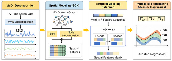
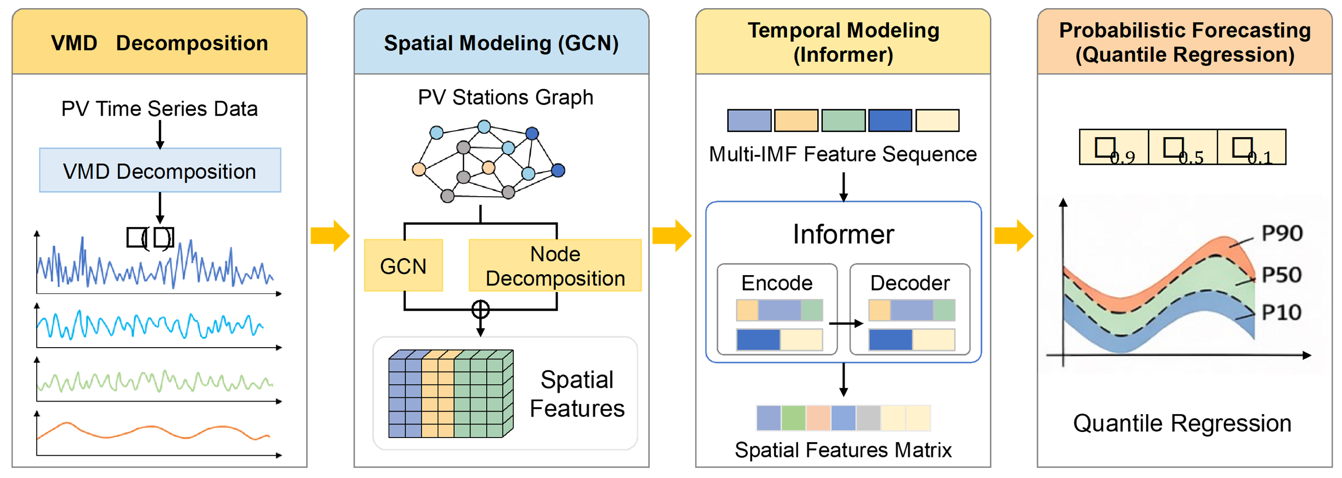
Figure 1 shows the overall framework of the proposed VMD–GCN–Informer–QR model. First, VMD is applied to decompose historical PV power time series into multiple intrinsic mode functions (IMFs), thereby reducing non-stationarity and noise interference. Next, a graph structure representing the spatial correlations among PV stations is constructed, and GCN is employed to extract spatial features from the decomposed modal components. Subsequently, the Informer model is introduced to efficiently capture long-term temporal dependencies. Finally, quantile regression is used to generate probabilistic forecasting results under multiple confidence levels.

Figure 1. The framework of VMD–GCN–Informer–QR model.

2.2. Variational Mode Decomposition for Time-Series Preprocessing

Due to fluctuations in meteorological conditions, PV power time series typically exhibit strong non-stationarity and multi-scale temporal characteristics. Directly feeding raw signals into deep learning models may lead to unstable training and degraded forecasting performance. To address this issue, VMD is introduced as a preprocessing method.

VMD decomposes the input signal into a predefined number of band-limited intrinsic mode functions (IMFs), each corresponding to oscillatory components in different frequency bands. For the original PV power signal $f\left(\omega \right)$, the decomposition process is formulated as a constrained variational optimization problem:

$${\widehat{\mu }}_k^{n+1}\left(\omega \right)={\displaystyle \frac{\widehat{f}\left(\omega \right)-\sum _{i=1,i<k}{\widehat{\mu }}_i^{n+1}(\omega )-\sum _{i=1,i>k}{\widehat{\mu }}_i^n(\omega )+\frac{{\widehat{\lambda }}^n}{2}(\omega )}{1+2\alpha {\left(\omega -{\omega }_k\right)}^2}}$$

(1)

$${\omega }_k^{n+1}={\displaystyle \frac{{\int }_0^{\infty }\omega {\left|{\widehat{\mu }}_k^{n+1}(\omega )\right|}^{2}d\omega }{{\int }_0^{\infty }{\left|{\widehat{\mu }}_k^{n+1}(\omega )\right|}^{2}d\omega }}$$

(2)

$${\widehat{\lambda }}^{n+1}\left(\omega \right)={\widehat{\lambda }}^n\left(\omega \right)+\gamma \left[\widehat{f}\left(\omega \right)-{\displaystyle \sum _{k=1}^K}{\widehat{\mu }}_k^{n+1}\left(\omega \right)\right]$$

(3)

$${\displaystyle \sum _{k=1}^K}({\displaystyle \frac{{‖{\widehat{\mu }}_k^{n+1}(\omega )-{\widehat{\mu }}_k^n(\omega )‖}_2^2}{{‖{\widehat{\mu }}_k^n(\omega )‖}_2^2}})<\epsilon$$

(4)

where $f\left(\omega \right)$ denotes the frequency-domain representation of the original PV power time series, and $\widehat{f}\left(\omega \right)$ is the corresponding Fourier transform; ${\widehat{\mu }}_k^{n+1}$ represents the frequency-domain representation of the k-th mode at the (n + 1)-th iteration; ${\omega }_k^{n+1}$ denotes the center frequency of the k-th mode at the (n + 1)-th iteration; ${\widehat{\lambda }}^n(\omega )$ is the Lagrange multiplier at the n-th iteration, enforcing the constraint that the sum of modes approximates the original signal; $\alpha$ is the penalty factor controlling the bandwidth compactness of each mode; $K$ denotes the number of decomposed modes; $\gamma$ is the step size for updating the Lagrange multiplier; $\epsilon$ is the convergence threshold for terminating the iteration.

Through iterative updates of the modes and their center frequencies, the original PV power sequence is decomposed into multiple IMFs, whose frequency ranges span from high-frequency fluctuations to low-frequency trends. These IMFs characterize the dynamic behavior of PV power from a multi-scale perspective and serve as enhanced input features for subsequent spatiotemporal modeling.

2.3. Graph Construction and Spatial Feature Extraction Using GCN

2.3.1. Graph Modeling of PV Station Clusters

In PV station clusters, stations are spatially distributed and influenced by similar meteorological conditions, leading to strong spatial correlations in their power outputs. To explicitly model such dependencies, the PV station cluster is represented as a graph $G=(V,E)$, where nodes $v_i\in \mathrm{V}$ represent individual PV stations and edges represent spatial relationships between stations.

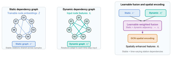
The proposed VMD–GCN–Informer–QR model employs a learnable dynamic–static fusion graph. The static graph represents stable dependencies among PV stations through trainable node embeddings, while the dynamic graph captures time-varying relationships from the input features at each time step. The two graph components are combined using a learnable fusion coefficient to obtain the adjacency matrix supplied to the GCN.

$$A^s=softmax\left(ReLU\left(Z{Z}^{\mathrm{T}}\right)\right)$$

(5)

$$Q_{\mathrm{t}}=X_{\mathrm{t}}{W}_Q$$

(6)

$$K_{\mathrm{t}}=X_{\mathrm{t}}{W}_K$$

(7)

$$A_t^d=softmax\left(Q_{\mathrm{t}}{K}_{\mathrm{t}}{\displaystyle \frac{\mathrm{T}}{\left|T_g\right|+\epsilon }}\right)$$

(8)

$$A_t={\alpha }_{g{A}^s}+\left(1-{\alpha }_g\right)A_t^d$$

(9)

$${\alpha }_g=sigmoid\left(\beta \right)$$

(10)

where $X_t$ denotes the node-feature matrix at time $t$; $Z$ is the trainable node-embedding matrix; $W_Q$ and $W_K$ are trainable projection matrices; $T_g$ is a learnable temperature parameter; and $\epsilon$ is a small positive constant ensuring numerical stability. $A^s$ and $A_t^d$ denote the static and dynamic adjacency matrices, respectively. The fusion coefficient ${\alpha }_g$ is obtained from the trainable parameter $\beta$ using the sigmoid function, and $A_t$ is the final adjacency matrix supplied to the GCN. The softmax operation is applied row-wise to normalize the connection weights of each node.

The dynamic–static dependency modeling process is illustrated in Figure 2. The learned static adjacency matrix $A^s$ and the input-dependent dynamic adjacency matrix $A_t^d$ are combined through the learnable fusion coefficient ${\alpha }_g$ to obtain $A_{\mathrm{t}}$. The fused adjacency matrix $A_t$, together with the node features $X_t$, is then supplied to the GCN for spatial feature extraction, and the extracted spatial features are subsequently passed to the Informer for temporal modeling.

Figure 2. Dynamic–static dependency modeling and learnable graph fusion framework.

2.3.2. Graph Convolutional Network

Based on the constructed graph structure, a Graph Convolutional Network (GCN) is employed to extract spatial features from the decomposed PV power signals. At each time step, the IMF components of all stations are used as node features and fed into the GCN.

The graph convolution operation at layer k + 1 can be expressed as:

$$X^{(l+1)}=h\left(D^{-{\displaystyle \frac{1}{2}}}A{D}^{-{\displaystyle \frac{1}{2}}}{X}^{\left(l\right)}\theta \right)$$

(11)

where $X^{\left(l\right)}$ denotes the feature matrix output by the l-th GCN layer; $X^{(l+1)}$ denotes the feature matrix output by the (l + 1)-th GCN layer; $A$ is the adjacency matrix describing spatial relationships among PV stations; $D$ is the corresponding degree matrix; $\theta$ is the learnable weight matrix; and $h(·)$ is the non-linear activation function.

Through neighborhood aggregation, the GCN enables each station to incorporate contextual information from spatially correlated stations, resulting in spatially enhanced feature representations.

2.4. Temporal Modeling with Informer

Informer is a variant of the Transformer architecture that retains the encoder–decoder structure while improving computational efficiency and long-sequence modeling capability through sparse self-attention, a distillation mechanism, and a generative decoder.

2.4.1. ProbSparse Self-Attention Mechanism

The self-attention mechanism in the standard Transformer is formulated as:

$$\mathrm{A}\mathrm{t}\mathrm{t}\mathrm{e}\mathrm{n}\mathrm{t}\mathrm{i}\mathrm{o}\mathrm{n}\left(Q,K,V\right)=Softmax\left({\displaystyle \frac{Q{K}^T}{\sqrt{d}}}\right)V$$

(12)

where $Q$, $K$, and $V$ denote the query, key, and value matrices, respectively; $Softmax$ is an activation function; and $d$ is the input dimension.

Informer improves upon the standard attention mechanism by exploiting the sparsity of attention distributions. It measures the divergence between the attention distribution of each query and a uniform distribution using the Kullback–Leibler divergence. The sparsity measurement for the i-th query is given by:

$$M\left(q_i,K\right)={max}_j\left({\displaystyle \frac{q_i{k}_j^T}{\sqrt{d}}}\right)-{\displaystyle \frac{1}{L}}{\displaystyle \sum _{j=1}^L}{\displaystyle \frac{q_i{k}_j^T}{\sqrt{d}}}$$

(13)

where $q_i$ denotes the i-th query vector, and $k_i$ represents the i-th value vector.

Dominant queries are then selected, and the attention is computed as:

$$\mathrm{A}\mathrm{t}\mathrm{t}\mathrm{e}\mathrm{n}\mathrm{t}\mathrm{i}\mathrm{o}\mathrm{n}\left(Q,K,V\right)=Softmax\left({\displaystyle \frac{\overline{Q}{K}^T}{\sqrt{d}}}\right)V$$

(14)

where $\overline{Q}$ denotes the matrix obtained from the original $Q$ after probabilistic sparsification. By retaining only the most relevant queries, this approach significantly reduces computational complexity and the dimensionality of the attention matrix.

2.4.2. Distillation Mechanism

The distillation mechanism introduces convolution and pooling operations between adjacent sparse self-attention layers to compress feature dimensions and emphasize dominant attention patterns:

$$X_{l+1}=\mathrm{M}\mathrm{a}\mathrm{x}\mathrm{p}\mathrm{o}\mathrm{o}\mathrm{l}\left(ELU\left(Conv1d{\left[X_l\right]}_{att}\right)\right)$$

(15)

where ${[ ]}_{att}$ denotes the attention block, and $Conv1d$ represents a one-dimensional convolution applied along the temporal dimension. A max-pooling layer is added after each convolution layer to downsample $X_l$ to half of its original length.

Through stacked sparse attention and distillation operations, the encoder captures long-term temporal dependencies. The generative decoder combines masked input sequences with learned temporal features via multi-head attention and directly outputs multi-step predictions, reducing decoding time and avoiding error accumulation.

2.4.3. Generative Decoder

The decoder receives input in the following form:

$$X_{dec}^i=Concat\left(X_{token}^i,X_0^i\right)\in R\left(L_{token}+T\right)\times d$$

(16)

where $X_{token}^i$ denotes the start token and $X_0^i$ represents the placeholder for the target sequence.

The input passes through the decoder, interacts with encoder features via cross-attention, and is finally processed by a fully connected layer to output all predicted values simultaneously.

2.5. Probabilistic Forecasting via Quantile Regression

Due to weather variability, the output of distributed PV systems exhibits significant uncertainty. For aggregated forecasting, such uncertainty should be represented in interval form. By integrating quantile regression with spatiotemporal graph neural networks, the model produces multiple quantile estimates and constructs prediction intervals representing aggregated uncertainty.

The essence of quantile regression is to transform the output of the spatiotemporal graph neural network into quantile estimates under different confidence levels. To avoid quantile crossing, an exponential stacking mapping is applied:

$$q_{i,{\mathrm{\kappa }}_r}=\left({\displaystyle \sum _{j=1}^r}{m}_{i,j}\right)-1$$

(17)

where based on the monotonicity of the exponential function, it is sufficient to ensure that $m_{i,j}\ge 0$ to guarantee that when ${\kappa }_r<{\kappa }_{r-1}$, the corresponding quantiles satisfy $q_{i,{\kappa }_r}<q_{i,{\kappa }_{r+1}}$.

After obtaining the aggregated quantile results, the loss function is computed. The Huber loss is adopted to characterize the loss of the uncertainty aggregation model. For a given quantile level ${\kappa }_r$, the Huber loss function is defined as follows:

$$L_H^r\left(y_{c,i},q_{i,{\kappa }_r}\right)=\left\{\begin{array}{c}{\kappa }_r\rho (y_{c,i},q_{i,{\kappa }_r},\eta ),y_{c,i}\ge q_{i,{\kappa }_r}\hfill \\ (1-{\kappa }_r)\rho (y_{c,i},q_{i,{\kappa }_r},\eta ),y_{c,i}<q_{i,{\kappa }_r}\hfill \end{array}\right.$$

(18)

where $y_{c,i}$ is the true value of the i^th sample; $\eta$ is a small positive constant; and $\rho \left(·\right)$ is the quantile deviation operator.

$$\rho \left(y_{c,i},q_{i,{\kappa }_r},\eta \right)=\left\{\begin{array}{c}\left|y_{c,i}-q_{i,{\kappa }_r}\right|-{\displaystyle \frac{\eta }{2}},\left|y_{c,i}-q_{i,{\kappa }_r}\right|\ge \eta \\ {\displaystyle \frac{{\left(y_{c,i}-q_{i,{\kappa }_r}\right)}^2}{2\eta }},\left|y_{c,i}-q_{i,{\kappa }_r}\right|<\eta \end{array}\right.$$

(19)

The final objective function of the aggregation model is:

$$min{\displaystyle \frac{1}{\left|\mathbb{Q}\right|\left|\mathbb{N}\right|}}\sum _{{\kappa }_r\in \mathbb{Q}}\sum _{i\in \mathbb{N}}{L}_H^{\left({\kappa }_r\right)}(y_{c,i},q_{i,{\kappa }_r})$$

(20)

where $\mathbb{N}$ denotes the dataset index set, $\mathbb{Q}$ denotes the set of quantile indices, and $\left|·\right|$ represents the indicator function.

3. Case Study

3.1. Data Description

The data were obtained from the Yulara Solar System operated by the Desert Knowledge Australia Solar Centre. The operator describes Yulara as an approximately 1.8-MW distributed PV facility and reports a total array rating of 1820 kW. The present study uses seven individual arrays with operator-reported ratings ranging from 22.56 to 1058.4 kW. The rated array capacity should be distinguished from the measured output: the Active_Power variable represents five-minute average AC active power and is expressed in kW. The forecasting target is the sum of the active-power measurements from the seven arrays and is therefore also reported in kW throughout this study. The analysed files span from 1 January 2019 at 08:00 to 1 February 2020 at 17:55. This interval covers 397 calendar days, of which 395 days are represented in the processed dataset. Each station contains exactly 47,400 temporally aligned observations. For each observed day, 120 five-minute records are retained between 08:00 and 17:55.

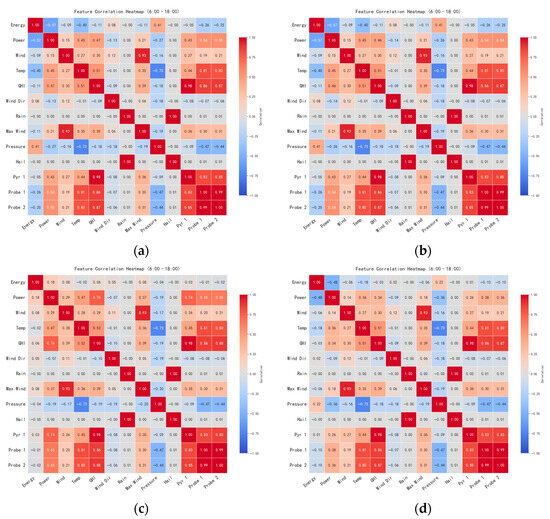
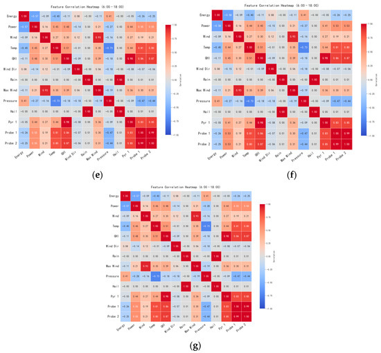
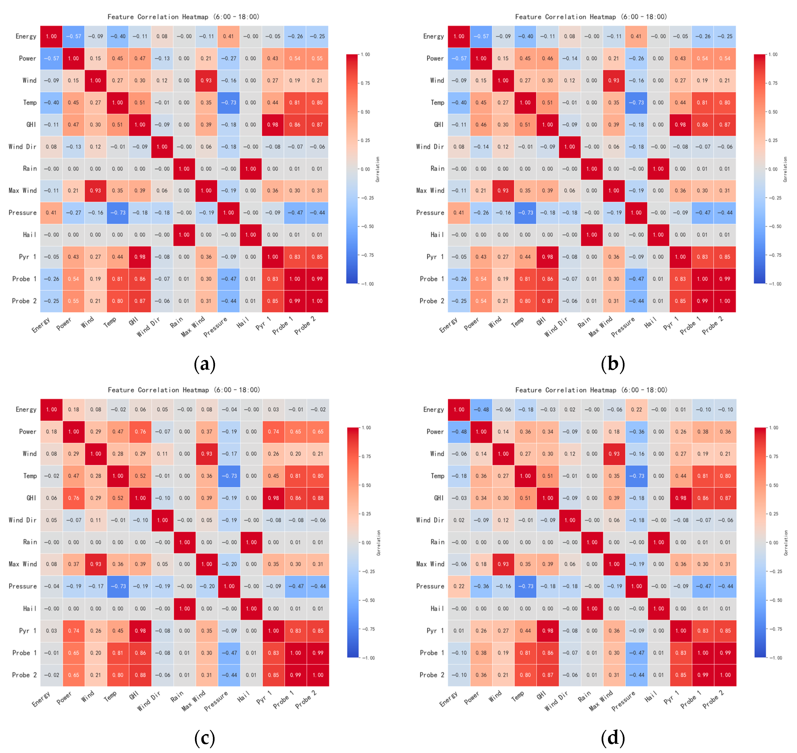
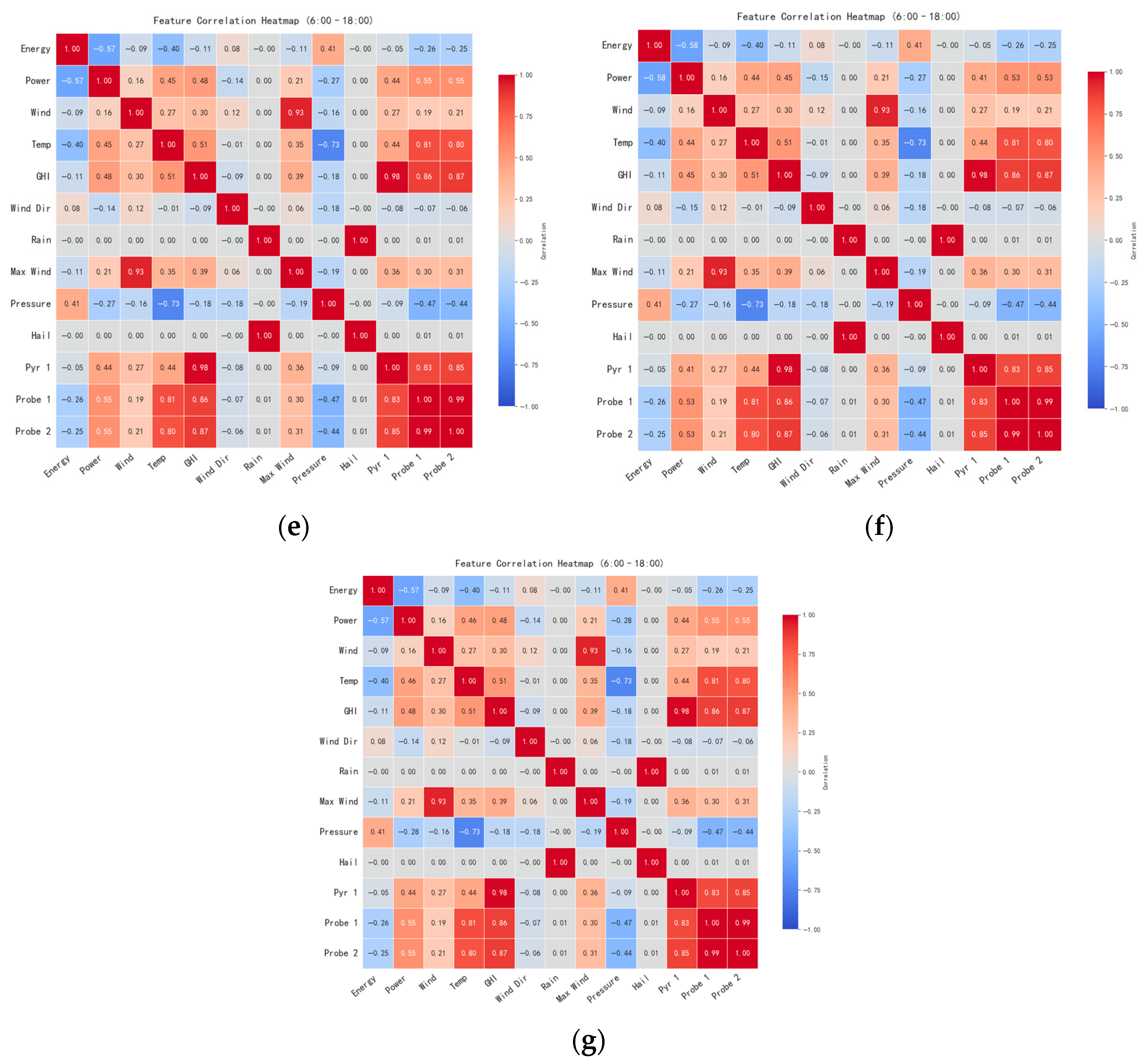
During the feature selection phase, Pearson correlation analysis is employed to quantify the linear relationships between individual features and the target variable. An absolute correlation coefficient threshold of 0.4 is applied to exclude features exhibiting weak correlations with the prediction target. Only features whose absolute correlation coefficients exceed this threshold across all sites are retained. The correlation heatmap illustrating the pairwise relationships among the candidate features and the target variable for the seven sites is presented in Figure 3. Consequently, the average current phase, insolation intensity, global horizontal irradiance, temperature, and active power are ultimately selected as input features for the model.

Figure 3. Heatmaps corresponding to the seven PV sites: (a) Site 1; (b) Site 2; (c) Site 3; (d) Site 4; (e) Site 5; (f) Site 6; (g) Site 7.

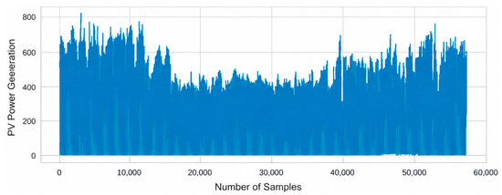
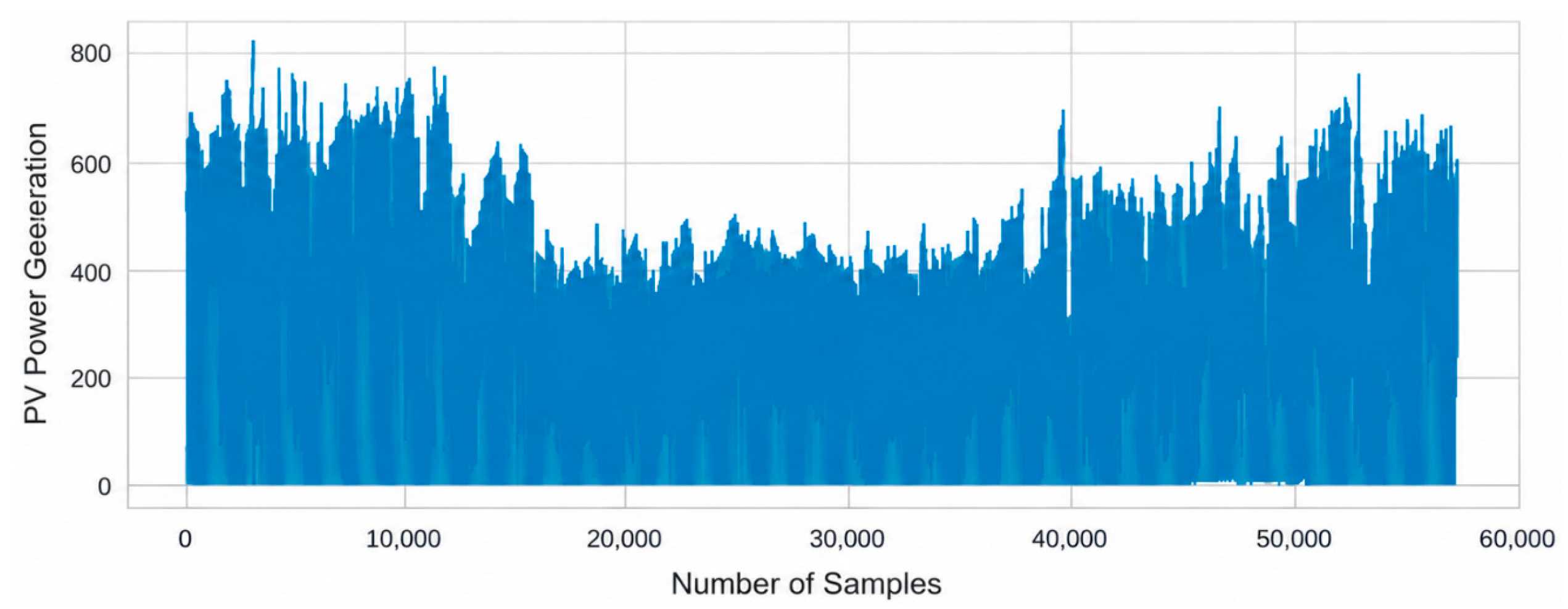
To further enhance the stability of model training, the input data are standardized, thereby aligning all features within a uniform numerical range and establishing a reliable data foundation for subsequent modeling. An illustrative subset of the data is shown in Figure 4.

Figure 4. Illustrative Subset of the Data.

Table 1 summarizes the photovoltaic power generation data from seven sites. The maximum, minimum, and mean values indicate obvious differences in generation capacity across sites. Site 1 shows the highest overall output, while Site 3 and Site 5 have relatively lower average generation. The minimum values close to zero reflect the intermittent nature of photovoltaic power generation.

Table 1. Descriptive statistics of active power at the seven PV systems (kW).

Site ID	Site 1	Site 2	Site 3	Site 4	Site 5	Site 6	Site 7
Maximum active power (kW)	821.59	46.85	23.04	104.38	37.29	208.43	296.84
Minimum active power (kW)	−0.16	−0.02	−0.02	−0.02	0.00	−0.04	−0.04
Mean active power (kW)	317.00	23.65	12.02	54.96	20.73	121.60	171.15

Each row in Table 2 represents the observations of one PV site at one timestamp. After temporal alignment, 24 consecutive records from each of the seven sites were stacked to construct an input tensor ${\mathbf{X}}_t\in {\mathbb{R}}^{24\times 7\times 6}$. The three dimensions represent 24 historical time steps, seven PV sites, and six input variables, respectively. The corresponding prediction target was the aggregate active power of the seven sites at the next five-minute time step.

Table 2. Representative records of the selected modeling dataset before normalization and VMD processing.

Timestamp	Mean Phase Current (A)	GHI ($\mathbf{W}·{\mathbf{m}}^{-2}$)	Pyranometer Irradiance ($\mathbf{W}·{\mathbf{m}}^{-2}$)	Temperature 1 (°C)	Temperature 2 (°C)	Active Power (kW)
1 January 2019 08:00	410.994	390.297	261.977	46.898	46.892	265.193
1 January 2019 08:05	440.053	411.274	296.037	47.383	47.307	284.259
1 January 2019 08:10	471.459	432.049	318.210	47.888	47.821	304.741

3.2. VMD

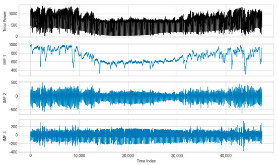
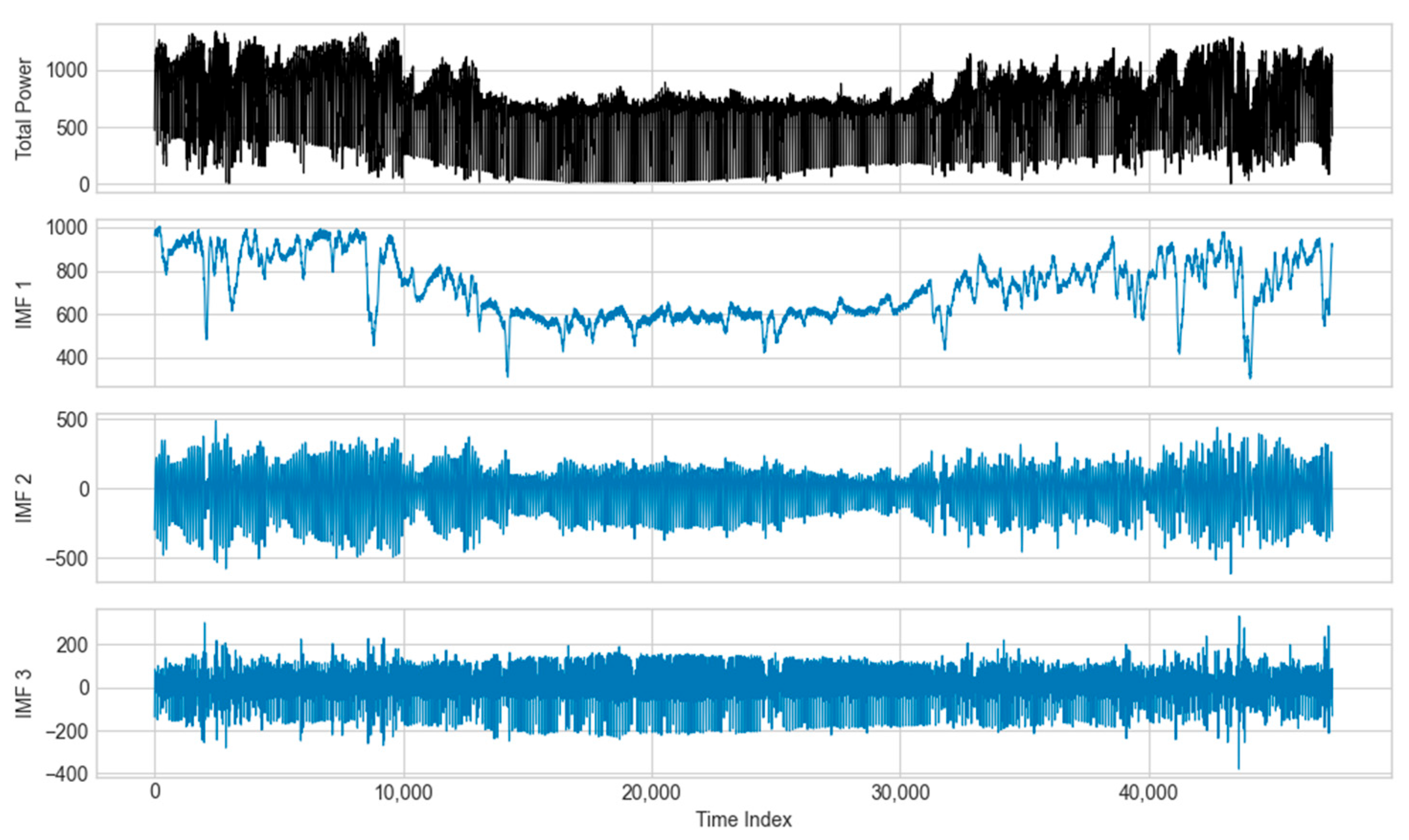
Variational Mode Decomposition was applied to separate the historical PV power sequence into components with different characteristic frequencies, as illustrated in Figure 5. To avoid subjective parameter assignment, the VMD configuration was selected through the training–validation procedure described in Section 2.2.

Figure 5. Decomposed IMF Components.

Among the retained configurations, $K=2$ and $\alpha =1000$ achieved the lowest mean validation loss across three independent training seeds, closely followed by $K=3$ and $\alpha =1000$, as shown in Figure S1 and Table S1 of the Supplementary Materials. Increasing $K$ reduced the reconstruction error in some cases but also decreased the convergence rate, whereas increasing $\alpha$ to 5000 degraded the downstream forecasting performance. These findings indicate that the suitable parameter region for the present dataset is concentrated around a small number of modes and $\alpha =1000$.

3.3. Graph Structure Construction

To evaluate the influence of graph construction, four graph structures were compared: a fixed binary Pearson graph, a weighted Pearson graph using the absolute correlation coefficients as edge weights, a dynamic-only graph, and the proposed dynamic–static fusion graph. All variants used the same chronological 70%/10%/20% data split, input features, forecasting architecture, optimization settings, and ten random seeds. Pearson-based graphs were constructed exclusively from the training set, whereas dynamic adjacency matrices were generated using only historical input features. A distance-based graph was not considered because reliable geographical coordinates were unavailable for all stations. The corresponding results are reported in Section 4.1.

3.4. Data Partitioning

The dataset was divided chronologically by complete calendar days into training, validation, and test partitions with proportions of 70%, 10%, and 20%, respectively. The first 276 days, from 1 January to 4 October 2019, were used for model training. The following 40 days, from 5 October to 14 November 2019, formed the validation set and were used for hyperparameter selection, validation-loss monitoring, and early stopping. The remaining 79 days, from 15 November 2019 to 1 February 2020, constituted the locked test set and were used only for final performance evaluation. No random shuffling was performed across the temporal partitions. The chronological split described above was used for the main full-period experiments. The seasonal experiments in Section 4.3 used separate season-specific chronological 70%/10%/20% splits.

3.5. Evaluation Metrics

This study evaluates model performance from the dual perspectives of point prediction and probabilistic prediction.

Point Prediction Evaluation Metrics include Mean Absolute Error (MAE) and Root Mean Square Error (RMSE), the formulas for which are presented as follows:

$$MAE={\displaystyle \frac{1}{N}}{\displaystyle \sum _{i=1}^N}\left|y_i-{\widehat{y}}_i\right|$$

(21)

$$RMSE=\sqrt{{\displaystyle \frac{1}{N}}{\displaystyle \sum _{i=1}^N}{\left(y_i-{\widehat{y}}_i\right)}^2}$$

(22)

where $y_i$ and ${\widehat{y}}_i$ represent the real and predicted value of sample $i$.

To enable scale-independent comparisons between PV systems with different output scales, the normalized mean absolute error (NMAE) and normalized root mean square error (NRMSE) are additionally employed:

$$NMAE={\displaystyle \frac{MAE}{P_{max}-P_{min}}}\times 100\%$$

(23)

$$NRMSE={\displaystyle \frac{RMSE}{P_{max}-P_{min}}}\times 100\%$$

(24)

where $P_{\mathrm{m}\mathrm{a}\mathrm{x}}$ and $P_{\mathrm{m}\mathrm{i}\mathrm{n}}$ denote the maximum and minimum values of the aggregate active power observed over the complete analyzed period of the corresponding dataset. NMAE and NRMSE are used only for scale-independent performance evaluation and do not participate in model training.

Probabilistic Prediction Evaluation Metrics include Prediction Interval Coverage Percentage (PICP) and Reliability Index.

Prediction Interval Coverage Percentage (PICP): $PICP$ represents the probability that the actual power value falls within the predicted fluctuation interval, thereby assessing the reliability of the forecasting model. It is expressed as:

$${PICP}_{\alpha }={\displaystyle \frac{100}{N}}{\displaystyle \sum _{i=1}^N}{c}_{i,\alpha }$$

(25)

where $c_{i,\alpha }$ denotes a Boolean variable. For sample $i$, $c_{i,\alpha }=1$ if the actual power value falls within the prediction interval corresponding to the given confidence level $a$; otherwise, $c_{i,\alpha }=0$. $\alpha$ denotes the prescribed confidence level.

Reliability Index ($R_a$): To further quantify the deviation between the empirical prediction interval coverage and the prescribed nominal coverage probability, the reliability index is defined as:

$$R_{\alpha }=I_{PICP,\alpha }-\alpha$$

(26)

A value of $R_{\alpha }$ close to zero indicates that the empirical coverage agrees well with the prescribed confidence level. A negative value indicates under-coverage, whereas a positive value indicates over-coverage.

Mean Prediction Interval Width (MPIW): MPIW reflects the average width between the upper and lower bounds of the prediction interval, and serves as a measure of the sharpness or concentration of the probabilistic forecasts. It is defined as:

$$\mathit{MPIW}={\displaystyle \frac{1}{N}}{\displaystyle \mathit{\sum }_{n=1}^N}{\delta }_n$$

(27)

where ${\delta }_n=L_{U,n}-L_{L,n}$ denotes the difference between the upper bound $L_{U,n}$ and lower bound $L_{L,n}$ for the n-th sample. The term ${\delta }_n$ quantifies the degree of concentration of the probabilistic prediction results.

The forecasting target is the aggregate active power of the seven PV systems, expressed in kW. Accordingly, MAE and RMSE are also expressed in kW. NMAE, NRMSE, PICP and the Reliability Index are reported as percentages, whereas the mean prediction interval width is expressed in kW.

4. Discussion

The input to the proposed model consists of six historical features, including global horizontal irradiance, solar irradiation, ambient temperature, and PV power, collected from seven PV stations. A sliding input window of 24 preceding time steps is used. Given the five-minute sampling interval, each input sample therefore covers the preceding 120 min. Specifically, the input tensor has the dimension $24\times 7\times 6$, corresponding to 24 historical time steps, seven PV stations, and six input features, respectively. For one-step-ahead forecasting, the model predicts the 0.1, 0.5, and 0.9 quantiles of the total regional PV power at the next time step, corresponding to a five-minute forecasting horizon. In the following, the parameters for the proposed model are listed in Table 3.

Table 3. Parameter settings of the proposed VMD–GCN–Informer–QR model.

Parameter Name	Value
Informer Hidden Layer Neurons	32
GCN Layers	2
Learning Rate	0.001
Optimizer	Adam
Number of Epochs	50
Loss Function	Quantile Regression Loss

4.1. Comparison with Benchmark Models

As shown in Table 4, Persistence provides a strong benchmark for 5-min-ahead PV power forecasting and achieves the lowest MAE of 40.590 kW. The proposed VMD-GCN-Informer-QR model obtains an MAE of 42.834 kW and the lowest RMSE of 72.182 kW, compared with 72.387 kW for Persistence. These results indicate that Persistence benefits from the strong short-term autocorrelation of PV power, whereas the proposed model is more effective in reducing relatively large forecasting errors.

Table 4. Metrics for different methods.

Model	MAE (kW)	RMSE (kW)	PICP (%)	${\mathbf{R}}_{\mathbf{a}}$ (%)	MPIW (kW)
Persistence	40.590	72.387
VMD-LSTM-QR	79.041	104.783	85.071	4.160	319.299
VMD-Informer-QR	84.796	110.505	89.960	7.062	397.479
VMD-GCN-LSTM-QR	45.797	73.839	89.532	5.871	199.467
VMD-GAT-Informer-QR	61.332	87.582	87.656	8.377	252.103
Proposed VMD-GCN-Informer-QR	42.834	72.182	89.682	4.756	201.818

In addition to point forecasts, the proposed model provides probabilistic prediction intervals, which are not available from the deterministic Persistence method. The proposed model obtains a PICP of 89.682%, close to the preset confidence level of 90%, with an MPIW of 201.818 kW. Therefore, although Persistence is highly competitive in terms of the 5-min-ahead MAE, the proposed model provides additional uncertainty information and achieves a favorable balance among RMSE, interval coverage, and interval width.

To further examine the influence of graph construction, the proposed fusion graph was compared with three alternative graph structures under identical experimental settings, as shown in Table 5.

Table 5. Forecasting performance of different graph construction methods.

Graph Structure	MAE (kW)	RMSE (kW)	PICP (%)	${\mathbf{R}}_{\mathbf{a}}$ (%)	MPIW (kW)
$\mathrm{Fixed} \mathrm{binary} \mathrm{Pearson} (\tau =0.60)$	83.338	109.414	89.955	6.328	389.653
Weighted Pearson	82.783	108.901	88.456	5.142	366.457
Dynamic-only	64.810	90.581	86.544	5.499	262.219
Proposed dynamic–static fusion	42.834	72.182	89.682	4.756	201.818

The proposed dynamic–static fusion graph achieved the lowest MAE and RMSE of 42.834 kW and 72.182 kW, respectively. Compared with the fixed binary Pearson, weighted Pearson, and dynamic-only graphs, it reduced MAE by 40.504, 39.949, and 21.976 kW, respectively. The corresponding differences were statistically significant after Holm correction (adjusted $p=0.0059$). These results indicate that jointly modeling stable and time-varying inter-station dependencies is more effective than using either a static correlation graph or a dynamic graph alone.

4.2. Discussion on Varying Output Horizons

To evaluate the forecasting performance and robustness of the proposed method over different lead times, four forecasting horizons of 15, 30, 45, and 60 min are considered. The original dataset has a sampling interval of 5 min, and the model generates forecasts for the subsequent 12 time steps. Therefore, the four reported forecasting horizons correspond to model output steps 3, 6, 9, and 12, respectively. At each forecasting horizon, point forecasting performance is evaluated using the Mean Absolute Error (MAE) and Root Mean Square Error (RMSE), while probabilistic forecasting performance is assessed using the Prediction Interval Coverage Probability (PICP), ${\mathrm{R}}_{\mathrm{a}}$, and Mean Prediction Interval Width (MPIW).

As shown in Table 6, the forecasting errors of all models generally increase as the forecasting horizon becomes longer, reflecting the greater uncertainty associated with longer lead times. Nevertheless, the proposed VMD–GCN–Informer–QR model achieves the lowest MAE and RMSE at all four forecasting horizons. At the 60-min horizon, the proposed method yields an MAE of 110.462 kW and an RMSE of 175.366 kW, whereas the second-best VMD–GCN–Informer–QR model obtains 116.984 kW and 182.191 kW, respectively. This corresponds to reductions of 5.58% in MAE and 3.75% in RMSE. These results indicate that, although the forecasting task becomes increasingly challenging as the prediction horizon extends, the proposed method maintains a consistent performance advantage over the competing models.

Table 6. Point forecasting performance of different methods under different forecasting horizons.

Model	Step 1 (kW)	Step 2 (kW)	Step 3 (kW)	Step 4 (kW)
Persistence	74.135/125.494	104.427/163.481	131.085/195.098	155.963/225.950
VMD-LSTM-QR	89.951/133.678	102.460/154.672	112.205/170.597	121.068/182.802
VMD-Informer-QR	92.063/134.382	103.364/153.998	112.616/169.645	121.835/182.992
VMD-GCN-LSTM-QR	81.911/129.774	95.555/151.981	106.505/168.817	116.984/182.191
VMD-GAT-Informer-QR	99.959/136.523	109.165/153.313	118.870/169.618	129.560/184.902
Proposed VMD-GCN-Informer-QR	68.095/117.036	88.166/144.314	101.125/162.225	110.462/175.366

Note: Values are reported as MAE/RMSE.

Table 7 further evaluates the probabilistic forecasting performance of the proposed method at different forecasting horizons. The PICP remains relatively stable across the four horizons, varying from 76.658% at 15 min to 75.243% at 60 min. In contrast, the MPIW increases progressively from 201.362 kW to 307.246 kW as the forecasting horizon extends. This increase in interval width is consistent with the greater uncertainty associated with longer-term forecasts. Meanwhile, the coverage increases from 1.911% to 3.133%. The results indicate that the proposed method maintains relatively stable prediction interval coverage across different forecasting horizons, while wider intervals are required to accommodate the increasing uncertainty of longer-horizon forecasting.

Table 7. Probabilistic forecasting performance of the proposed VMD–GCN–Informer–QR model under different forecasting horizons.

Horizon	PICP (%)	${\mathit{R}}_{\mathit{a}}$ (%)	MPIW (kW)
15 min	76.658	1.911	201.362
30 min	75.163	2.651	244.888
45 min	75.193	3.120	277.485
60 min	75.243	3.133	307.246

4.3. Discussion on Seasonal Variation

PV power forecasting performance is affected by seasonal variations in solar irradiance and meteorological conditions. Following the conventional meteorological seasons in Australia, spring is defined as September to November, summer as December to February, autumn as March to May, and winter as June to August. To evaluate the robustness and generalization capability of the proposed VMD–GCN–Informer–QR model under different seasonal conditions, the test samples are grouped according to the four seasons, and the corresponding point and probabilistic forecasting metrics are calculated separately. The results are summarized in Table 8.

Table 8. Metrics for VMD–GCN–Informer–QR of different seasons.

Season	MAE (kW)	RMSE (kW)	PICP (%)	${\mathbf{R}}_{\mathbf{a}}$ (%)	MPIW (kW)
Spring	50.706	75.437	81.765	3.754	182.101
Summer	52.938	81.705	90.858	7.279	241.431
Autumn	45.869	64.942	90.055	10.613	182.698
Winter	21.364	28.303	85.055	7.004	88.786

As shown in Table 8, the forecasting performance of the proposed VMD–GCN–Informer–QR model exhibits clear seasonal variations. Winter achieves the lowest point forecasting errors, with an MAE of 21.364 kW and an RMSE of 28.303 kW, followed by autumn, with an MAE of 45.869 kW and an RMSE of 64.942 kW. In comparison, spring and summer exhibit relatively larger errors, with MAE values of 50.706 and 52.938 kW and RMSE values of 75.437 and 81.705 kW, respectively. These results indicate that the predictability of PV power varies considerably across seasons, which may be associated with seasonal differences in irradiance patterns and meteorological variability.

For probabilistic forecasting, the PICP values are 81.765%, 90.858%, 90.055%, and 85.055% for spring, summer, autumn, and winter, respectively. Summer achieves the highest interval coverage, but it also has the largest prediction interval width, with an MPIW value of 241.431 kW. In contrast, winter combines a PICP of 85.055% with the narrowest prediction interval of 88.786 kW. Autumn provides relatively high interval coverage of 90.055% with a moderate interval width of 182.698 kW, whereas spring presents the lowest PICP of 81.765%. These results highlight the trade-off between prediction interval coverage and interval width across different seasons. Although the forecasting performance varies with seasonal conditions, the proposed method maintains effective point forecasting and uncertainty quantification capabilities throughout the year.

4.4. External-Region Multi-Site Validation

To evaluate the cross-region applicability of the proposed framework, an additional experiment was conducted using the Alice Springs 1B dataset. Seven independently monitored PV arrays were treated as graph nodes. After data cleaning and daylight filtering, 386 complete days with 46,320 five-minute observations per node were retained and chronologically divided into training, validation, and test sets of 270, 38, and 78 days, respectively.

Both models were retrained on the Alice Springs data using the same preprocessing, input window, model configuration, and one-step-ahead setting as in Table 4, corresponding to a 5-min forecasting horizon. The graph was reconstructed using only the Alice Springs training data. Each model was independently trained three times, and the mean results are reported. Because the two datasets have different power scales, NMAE and NRMSE were additionally used for cross-dataset comparison.

As shown in Table 9, the proposed model achieved an NMAE of 4.476% and an NRMSE of 7.379% on the Alice Springs dataset, compared with 3.190% and 5.376% on the Yulara dataset. Although the normalized errors increased by 40.31% and 37.26%, respectively, they remained within the same order of magnitude. On the Alice Springs dataset, the proposed model obtained a slightly lower RMSE but a slightly higher MAE than VMD-Informer-QR. Therefore, the results support the adaptability of the framework to a new regional PV network, although graph modeling did not improve every point forecasting metric at the 5-min horizon.

Table 9. External-region validation under the same one-step-ahead forecasting setting as Table 4.

Dataset	Model	MAE (kW)	RMSE (kW)	NMAE (%)	NRMSE (%)
Yulara	VMD–Informer–QR	84.796	110.505	6.315	8.230
Yulara	Proposed VMD–GCN–Informer–QR	42.834	72.182	3.190	5.376
Alice Springs	VMD–Informer–QR	2.145	3.668	4.320	7.387
Alice Springs	Proposed VMD–GCN–Informer–QR	2.222	3.664	4.476	7.379

5. Conclusions

To address the challenges of strong non-stationarity, insufficient spatial correlation modeling, long-term dependency extraction, and uncertainty quantification in PV plant cluster forecasting, this paper proposes a spatiotemporal probabilistic forecasting framework integrating VMD, GCN, Informer, and quantile regression. The proposed framework combines multi-scale decomposition, spatial feature extraction, temporal dependency modeling, and probabilistic forecasting to improve the forecasting performance of PV plant clusters.

(1) At the 5-min forecasting horizon, Persistence achieves the lowest MAE of 40.590 kW. Although the proposed VMD–GCN–Informer–QR model obtains a slightly higher MAE of 42.834 kW, it achieves the lowest RMSE of 72.182 kW and provides probabilistic forecasts with a PICP of 89.682% and an MPIW of 201.818 kW. These results demonstrate its ability to limit large forecasting errors while providing useful uncertainty information.

(2) In multi-step forecasting, the proposed method consistently achieves the lowest MAE and RMSE across forecasting horizons from 15 to 60 min. At the 60-min horizon, the MAE and RMSE are 110.462 kW and 175.366 kW, respectively, demonstrating its effectiveness for longer forecasting horizons.

(3) Seasonal experiments show that the forecasting performance varies across different seasons. The lowest prediction errors are obtained in winter, with an MAE of 21.364 kW and an RMSE of 28.303 kW. Overall, the proposed method maintains effective point forecasting and uncertainty quantification capabilities under different seasonal conditions.

(4) External-region validation using seven PV array-level nodes from the Alice Springs 1B system shows that the proposed model achieves NMAE values of 3.190% and 4.476% and NRMSE values of 5.376% and 7.379% on the Yulara and Alice Springs datasets, respectively. These results support the adaptability of the proposed framework to external regional PV data after retraining.

References

- Kannan, N.; Vakeesan, D. Solar energy for future world: A review. Renew. Sustain. Energy Rev. 2016, 62, 1092–1105. [Google Scholar] [CrossRef] [Scilit]
- Das, U.K.; Tey, K.S.; Seyedmahmoudian, M.; Mekhilef, S.; Idris, M.Y.I.; Deventer, W.V.; Horan, B.; Stojcevski, A. Forecasting of photovoltaic power generation and model optimization: A review. Renew. Sustain. Energy Rev. 2018, 81, 912–928. [Google Scholar] [CrossRef] [Scilit]
- Larson, D.; Coimbra, C. Direct power output forecasts from remote sensing image processing. J. Sol. Energy Eng. 2018, 140, 021011. [Google Scholar] [CrossRef] [Scilit]
- Alsharif, M.H.; Younes, M.K.; Kim, J. Time series ARIMA model for prediction of daily and monthly average global solar radiation: The case study of Seoul, South Korea. Symmetry 2019, 11, 240. [Google Scholar] [CrossRef] [Scilit]
- Shakya, A.; Michael, S.; Saunders, C.; Armstrong, D.; Pandey, P.; Chalise, S.; Tonkoski, R. Solar irradiance forecasting in remote microgrids using Markov switching model. IEEE Trans. Sustain. Energy 2017, 8, 895–905. [Google Scholar] [CrossRef]
- Chodakowska, E.; Nazarko, J.; Nazarko, Ł.; Rabayah, H.S.; Abendeh, R.M.; Alawneh, R. ARIMA models in solar radiation forecasting in different geographic locations. Energies 2023, 16, 5029. [Google Scholar] [CrossRef] [Scilit]
- Benghanem, M.; Mellit, A. Radial Basis Function Network-based prediction of global solar radiation data: Application for sizing of a stand-alone photovoltaic system at Al-Madinah, Saudi Arabia. Energy 2010, 35, 3751–3762. [Google Scholar] [CrossRef] [Scilit]
- Eseye, A.T.; Zhang, J.; Zheng, D. Short-term photovoltaic solar power forecasting using a hybrid Wavelet-PSO-SVM model based on SCADA and Meteorological information. Renew. Energy 2018, 118, 357–367. [Google Scholar] [CrossRef] [Scilit]
- Mellit, A.; Benghanem, M.; Kalogirou, S.A. Modeling and simulation of a stand-alone photovoltaic system using an adaptive artificial neural network: Proposition for a new sizing procedure. Renew. Energy 2007, 32, 285–313. [Google Scholar] [CrossRef] [Scilit]
- Li, G.; Wang, H.; Zhang, S.; Xin, J.; Liu, H. Recurrent neural networks based photovoltaic power forecasting approach. Energies 2019, 12, 2538. [Google Scholar] [CrossRef] [Scilit]
- Wang, Y.; Liao, W.; Chang, Y. Gated recurrent unit network-based short-term photovoltaic forecasting. Energies 2018, 11, 2163. [Google Scholar] [CrossRef] [Scilit]
- Son Huu, V.X.; Hieu, D.D.; Minh Giang, N.H.; Takano, H.; Tuyen, N.D. Deep learning-based real-time solar irradiation monitoring and forecasting application for PV system. In Proceedings of the 2023 7th International Conference on Green Energy and Applications (ICGEA), Singapore, 10–12 March 2023; pp. 40–45. [Google Scholar] [CrossRef] [Scilit]
- Wang, F.; Xuan, Z.; Zhen, Z.; Li, K.; Wang, T.; Shi, M. A day-ahead PV power forecasting method based on LSTM-RNN model and time correlation modification under partial daily pattern prediction framework. Energy Convers. Manag. 2020, 212, 112766. [Google Scholar] [CrossRef] [Scilit]
- Zhou, H.; Zhang, S.; Peng, J.; Zhang, S.; Li, J.; Xiong, H.; Zhang, W. Informer: Beyond efficient transformer for long sequence time-series forecasting. In Proceedings of the Thirty-Fifth AAAI Conference on Artificial Intelligence, Thirty-Third Conference on Innovative Applications of Artificial Intelligence and the Eleventh Symposium on Educational Advances in Artificial Intelligence, Virtual, 2–9 February 2021; Volume 35, pp. 11106–11115. [Google Scholar]
- Kushwaha, V.; Pindoriya, N. A SARIMA-RVFL hybrid model assisted by wavelet decomposition for very short-term solar PV power generation forecast. Renew. Energy 2019, 140, 124–139. [Google Scholar] [CrossRef] [Scilit]
- Niu, D.; Wang, K.; Sun, L.; Wu, J.; Xu, X. Short-term photovoltaic power generation forecasting based on random forest feature selection and CEEMD: A case study. Appl. Soft Comput. 2020, 93, 106389. [Google Scholar] [CrossRef] [Scilit]
- Tang, H.; Kang, F.; Li, X.; Sun, Y. Short-term photovoltaic power prediction model based on feature construction and improved transformer. Energy 2025, 320, 135213. [Google Scholar] [CrossRef] [Scilit]
- Li, B.; Wang, H.; Zhang, J. Short-term power forecasting of photovoltaic generation based on CFOA-CNN-BiLSTM-Attention. Electr. Eng. 2025, 107, 10335–10347. [Google Scholar] [CrossRef] [Scilit]
- Wang, T.; Liu, Z.; Sheng, C.; Guo, W. SHapley additive exPlanations-based neural architecture search and multi-channel temporal convolutional network with bidirectional gated recurrent unit-based photovoltaic power ultra-short-term fusion prediction with abrupt weather feature enhancement. Electr. Power Syst. Res. 2026, 255, 112694. [Google Scholar] [CrossRef] [Scilit]
- Zhang, M.; Zhen, Z.; Liu, N.; Zhao, H.; Sun, Y.; Feng, C.; Wang, F. Optimal graph structure based short-term solar PV power forecasting method considering surrounding spatio-temporal correlations. IEEE Trans. Ind. Appl. 2023, 59, 345–357. [Google Scholar] [CrossRef] [Scilit]
- Yang, C.; Li, S.; Gou, Z. Spatiotemporal prediction of urban building rooftop photovoltaic potential based on GCN-LSTM. Energy Build. 2025, 334, 115522. [Google Scholar] [CrossRef] [Scilit]
- Zhuang, W.; Li, Z.; Wang, Y.; Xi, Q.; Xia, M. GCN–Informer: A novel framework for mid-term photovoltaic power forecasting. Appl. Sci. 2024, 14, 2181. [Google Scholar] [CrossRef] [Scilit]
- Massaoudi, M.; Chihi, I.; Sidhom, L.; Trabelsi, M.; Refaat, S.S.; Abu-Rub, H.; Oueslati, F.S. An effective hybrid NARX-LSTM model for point and interval PV power forecasting. IEEE Access 2021, 9, 36571–36588. [Google Scholar] [CrossRef] [Scilit]
- Gu, B.; Shen, H.; Lei, X.; Hu, H.; Liu, X. Forecasting and uncertainty analysis of day-ahead photovoltaic power using a novel forecasting method. Appl. Energy 2021, 299, 117291. [Google Scholar] [CrossRef] [Scilit]
- Van Der Meer, D.W.; Shepero, M.; Svensson, A.; Widén, J.; Munkhammar, J. Probabilistic forecasting of electricity consumption, photovoltaic power generation and net demand of an individual building using Gaussian Processes. Appl. Energy 2018, 213, 195–207. [Google Scholar] [CrossRef] [Scilit]
- Wang, H.; Yi, H.; Peng, J.; Wang, G.; Liu, Y.; Jiang, H.; Liu, W. Deterministic and probabilistic forecasting of photovoltaic power based on deep convolutional neural network. Energy Convers. Manag. 2017, 153, 409–422. [Google Scholar] [CrossRef] [Scilit]
- Alfredo Fernandez-Jimenez, L.; Terreros-Olarte, S.; Mendoza-Villena, M.; Garcia-Garrido, E.; Zorzano-Alba, E.; Lara-Santillan, P.M.; Zorzano-Santamaria, P.J.; Falces, A. Day-ahead probabilistic photovoltaic power forecasting models based on quantile regression neural networks. In Proceedings of the 2017 European Conference on Electrical Engineering and Computer Science (EECS), Bern, Switzerland, 17–19 November 2017; pp. 289–294. [Google Scholar] [CrossRef] [Scilit]
- Ma, X.; Du, H.; Wang, K.; Jia, R.; Wang, S. An efficient QR-BiMGM model for probabilistic PV power forecasting. Energy Rep. 2022, 8, 12534–12551. [Google Scholar] [CrossRef] [Scilit]
Disclaimer/Publisher’s Note: The statements, opinions and data contained in all publications are solely those of the individual author(s) and contributor(s) and not of MDPI and/or the editor(s). MDPI and/or the editor(s) disclaim responsibility for any injury to people or property resulting from any ideas, methods, instructions or products referred to in the content. |
© 2026 by the authors. Licensee MDPI, Basel, Switzerland. This article is an open access article distributed under the terms and conditions of the Creative Commons Attribution (CC BY) license.