


Abstract
The hybrid operation of grid-following (GFL) and grid-forming (GFM) renewable energy units can lead to phase-reference inconsistencies and distorted transient impedance trajectories, which in turn cause maloperation or failure-to-operate of conventional distance protection. To address this issue, this paper proposes a novel distance protection method based on transient impedance fitting. First, a dynamic phase transformation is applied to map the currents of GFL units into a unified reference frame, enabling consistent representation of heterogeneous currents from the hybrid renewable energy station. Second, a transient equivalent impedance model is established based on the transient voltage-current relationship of the transmission line, revealing the influence mechanisms of the rates of change in current amplitude and phase angle on the transient additional impedance. Finally, the magnitude of the transient impedance within a short post-fault data window is selected as the fitting object. The least-squares method is employed to extract the linear fitting slope and intercept, which characterize the evolution trend and initial position of the transient impedance trajectory, respectively, thereby forming the criteria for distinguishing internal and external faults. Simulation results demonstrate that the proposed method correctly identifies fault sections under various fault locations, transition resistances, and renewable power output conditions, with the protection decision completed within 15 ms. The proposed method effectively overcomes the susceptibility of conventional distance protection to maloperation and failure-to-operate in scenarios with high renewable energy penetration.
1. Introduction
With the increasingly prominent “dual-high” characteristics of new-type power systems, the large-scale integration of renewable energy stations into the grid via AC transmission lines has become a typical operational scenario. Compared with traditional synchronous sources, renewable energy sources are grid-connected through power electronic converters, and their fault transient outputs are jointly influenced by control strategies, current-limiting links, and low-voltage ride-through (LVRT) controls. The resulting short-circuit currents exhibit non-traditional features such as amplitude limitation, frequency deviation, and phase controllability, which lead to adaptability degradation of conventional protection principles based on power-frequency steady-state phasors [1,2,3,4,5,6]. As a critical protection configuration for transmission lines, distance protection relies on the phasor relationship among measured voltage, current, and line impedance. However, in renewable-energy-integrated scenarios, both the amplitude and phase angle of fault currents are constrained by inverter control loops, causing measured impedance to deviate, which may in turn result in maloperation—either refusal to trip for internal faults or incorrect tripping for external faults [7,8,9].
Distance protection, as the primary protection for transmission lines, determines the fault location by measuring the electrical distance from the relay installation point to the fault point. Depending on the measurement principle and the criteria of the measured quantity, three classic schemes are widely adopted in engineering practice: impedance protection, reactance protection, and admittance protection. The impedance protection scheme compares the measured impedance with a preset threshold. Zone 1 is typically set to 80–85% of the line impedance, forming an underreaching characteristic that enables instantaneous tripping without time delay coordination. The reactance protection scheme identifies faults by measuring the reactance component. Since the fault reactance is mainly proportional to the line reactance and is less affected by the transition resistance, this scheme exhibits strong capability in withstanding high-resistance faults. However, its inability to effectively distinguish the resistance component makes it susceptible to load encroachment and reverse faults. The admittance protection scheme identifies faults by measuring the admittance. It offers certain advantages in overcoming power oscillations and current transformer saturation, but its dependence on voltage magnitude makes it vulnerable under weak-infeed conditions. In conventional power systems dominated by synchronous generators, the above three schemes have been well-developed and complement each other. However, in the hybrid integration scenario of grid-following (GFL) and grid-forming (GFM) renewable energy units, the fault currents exhibit characteristics such as amplitude limitation, phase controllability, and inconsistent reference frames, which severely undermine the physical assumptions underlying these classic schemes, making it difficult to ensure reliable operation.
To address the adaptability deficiency of distance protection after renewable energy integration, considerable research has been conducted. On one hand, some studies start from the analytical derivation of renewable fault currents, establishing transient current models that incorporate phase-locked loops (PLLs), inner current loops, and LVRT strategies, thereby revealing the amplitude limitation, phase deviation, and sequence-component variation patterns of inverter-interfaced source fault currents [10,11,12,13]. These works provide a theoretical foundation for analyzing fault characteristics of renewable transmission lines; however, most methods are primarily targeted at single GFL sources and cannot directly reflect the coupling effects of dynamic responses among different units in hybrid stations with multiple control modes. On the other hand, to address measured impedance deviation and insufficient protection sensitivity under high-resistance faults, improved schemes such as adaptive distance protection, additional impedance compensation, control–protection coordination, and voltage-memory-based directional criteria have been proposed [14,15,16]. Although these approaches improve the performance of conventional distance protection under renewable integration to some extent, they still suffer from limitations such as dependence on specific control strategies, complex setting procedures, or inadequate adaptability to varying system operating conditions.
With the advancement of GFM renewable technologies, the hybrid integration of GFL and GFM units has gradually become an important trend in large-scale renewable stations. GFL units typically rely on PLLs to obtain the phase of the point of common coupling (PCC) voltage and externally behave as controlled current sources; GFM units, in contrast, establish their own phase reference through virtual inertia, damping, and voltage control loops, and externally behave as controlled voltage sources [17,18,19]. The two types of units differ significantly in synchronization mechanisms, fault ride-through modes, and current-limiting strategies, leading to inconsistent phase reference bases for the fault-current feed during transients. If currents from different local reference frames are directly used for line current synthesis and impedance calculation, the original physical mapping between voltage and current becomes disrupted, causing further distortion of the measured impedance trajectory. Particularly under high-resistance faults, weak-infeed operation, and fluctuating renewable power outputs, the aforementioned phase-reference mismatch, superimposed on the controlled fault-current characteristics, makes it even harder to maintain stable operating boundaries for conventional distance protection.
Existing studies on protection adaptability for GFM sources mainly focus on fault current characteristics, current-limiting strategies, and control–protection coordination methods [20,21]. Some studies have already addressed the impact of GFM units on distance protection, pointing out that their voltage-source characteristics, current-limiting modes, and fault-ride-through controls alter the impedance trajectory perceived by the relay, potentially leading to overreach or underreach of distance protection. However, for transmission lines emanating from hybrid GFL/GFM renewable stations, two deficiencies remain in the existing literature: first, most methods have not fully considered the influence of phase-reference differences between the two unit types on the synthesized line current and measured impedance; second, some protection criteria still rely mainly on post-fault single-point impedance or power-frequency steady-state phasors, which cannot effectively characterize the overall evolution of transient impedance trajectories during the early fault stage. Therefore, there is an urgent need to develop a novel distance protection method that can accommodate the heterogeneous current characteristics of hybrid renewable stations and utilize the evolving trend of transient impedance to discriminate fault sections.
To provide a clear overview of the existing research foundation, representative studies are summarized and compared in Table 1.
Table 1.
Comparison of representative studies on distance protection for renewable energy transmission lines.
From Table 1, it can be seen that existing studies have achieved certain progress in scenarios with single-type GFL or GFM integration. However, for transmission lines emanating from hybrid GFL/GFM renewable energy stations, the following deficiencies remain. First, most methods have not fully considered the phase-reference inconsistency caused by the distinct control strategies of the two unit types, making it difficult to accurately characterize the synthesized current of hybrid stations. Second, some protection criteria still rely on steady-state fundamental components or single-point impedance measurements after fault inception, which are inadequate to capture the overall evolution of transient impedance trajectories during the early fault stage. Based on the above analysis, this paper proposes a novel distance protection method based on transient impedance fitting.
To address the above issues, this paper proposes a novel distance protection scheme based on transient impedance fitting. The main contributions of this paper can be summarized as follows.
- By selecting the phase of the GFM unit as the unified reference and applying dynamic phase transformation to map the currents of the GFL units into this unified reference frame, the phase inconsistency of heterogeneous currents in the hybrid renewable energy station is effectively resolved, enabling coherent synthesis of heterogeneous currents in a unified reference frame.
- A transient equivalent impedance model is established under the unified reference frame, which decomposes the impedance variation during faults into a steady-state setting impedance and a time-varying transient additional impedance, revealing the influence mechanisms of the rates of change in current amplitude and phase angle on the transient impedance trajectory.
- The least squares method is adopted to perform linear fitting on the transient impedance magnitude within a short post-fault data window, extracting the slope that characterizes the evolution trend of the impedance trajectory and the intercept that characterizes its initial position, thereby forming a criterion for distinguishing internal and external faults that does not rely on steady-state fundamental frequency impedance.
- Extensive simulations are conducted in PSCAD/EMTDC under various fault locations, fault types, transition resistances (50 Ω to 200 Ω), and renewable power outputs (25 MW to 100 MW). The results demonstrate that the proposed scheme can correctly identify fault sections, and the protection operating time is consistently less than 15 ms.
- The proposed method effectively overcomes the susceptibility of conventional distance protection to maloperation and failure to operate in high renewable penetration scenarios, demonstrating strong adaptability and promising engineering application prospects.
The remaining content of this article is as follows. Section 2 analyzes the transient output characteristics of hybrid renewable energy stations and the limitations of conventional distance protection. Section 3 presents the proposed distance protection scheme based on transient impedance fitting, including the establishment of a unified reference frame, the definition of transient equivalent impedance, and the construction of the fitting-based criterion. Section 4 conducts comprehensive simulation verification under various fault locations, fault types, transition resistances, and renewable power outputs to validate the effectiveness and adaptability of the proposed method. The conclusion is drawn in Section 5.
2. Transient Output Characteristics of Hybrid Renewable Energy Stations and Limitations of Conventional Distance Protection
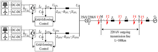
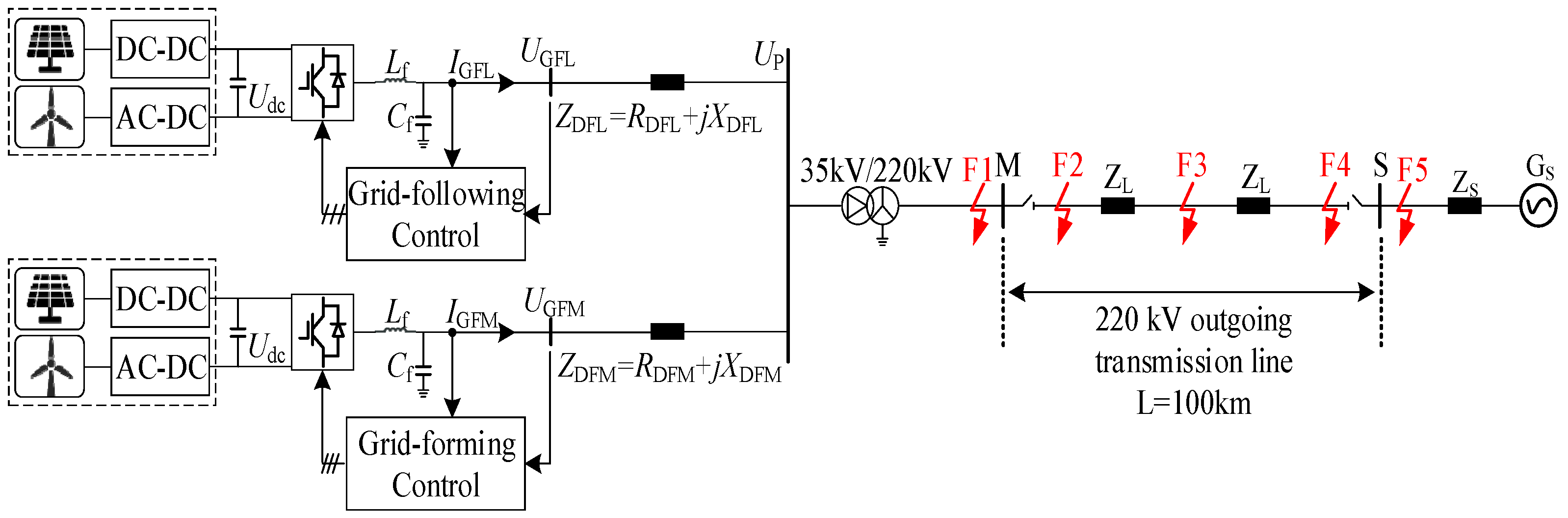
In the context of power systems with a high penetration of renewable energy and power electronic converters, the hybrid integration of GFL and GFM converter-based units has become a typical configuration for large-scale renewable stations. The topology of the hybrid renewable energy transmission system is shown in Figure 1.
Figure 1.
Topology of the Combined Hybrid New Energy Station Transmission System.
As shown in Figure 1, renewable energy sources are aggregated through hybrid GFL and GFM inverters. The aggregated power is stepped up by a main transformer and delivered to the main grid through an AC transmission line. Points M and S represent the locations where distance protection relays are installed at both ends of the transmission line. Faults F2–F4 denote internal faults, while F1 and F5 correspond to reverse and forward external faults, respectively. During the fault transient, the distinct control strategies of GFL and GFM units lead to heterogeneous dynamic responses in their output currents. These heterogeneous responses are coupled and superimposed at the point of common coupling, resulting in nonlinear distortions of the composite short-circuit electrical quantities of the transmission line. Consequently, conventional distance protection faces potential risks of maloperation or failure to operate.
2.1. Transient Output Characteristics and Phase Misalignment Mechanism of Hybrid Renewable Energy Stations
Since a hybrid renewable energy station consists of both GFL and GFM units, the phase reference frames of their fault currents are fundamentally different due to the distinct control structures.
GFL and GFM units exhibit fundamentally different external characteristics during transients due to their distinct control objectives and synchronization mechanisms. Therefore, different equivalent models must be adopted in system analysis.
The GFL unit relies on the PLL as its core synchronization element. Its control objective is to rapidly track the phase and frequency of the PCC voltage, with the output current strictly following the inner current-loop references. During fault transients, the current-limiting link restricts the output current amplitude to within 1.2–2.0 times its rated value, resulting in a controlled current source characteristic with controllable magnitude and phase. Therefore, from the grid’s perspective, the GFL unit can be equivalently represented as a controlled current source.
In contrast, the GFM unit autonomously establishes its voltage reference phase by emulating the swing equation of a synchronous generator (virtual inertia and damping), and maintains the internal EMF magnitude through voltage-loop control. Its output voltage is actively set by the control strategy, while the output current is naturally determined by the network impedance and the voltage difference. Therefore, from the grid’s perspective, the GFM unit can be equivalently represented as a controlled voltage source.
The difference between the above equivalent models directly leads to the inconsistency in the phase reference bases of fault currents between the two unit types—the phase of the GFL unit depends on the PLL tracking of the PCC voltage, whereas the phase of the GFM unit is autonomously determined by the virtual inertia loop. This fundamental discrepancy in phase reference is the primary motivation for proposing the dynamic phase conversion method in this paper.
2.1.1. Grid-Following Renewable Energy Station
A GFL unit can be equivalently represented as a controlled current source from the grid perspective. Its transient response is determined by the voltage at the point of common coupling and the internal control loops. When the PCC voltage experiences a severe voltage sag, the unit enters the LVRT control mode. In contrast, when the voltage drop is relatively mild, the original active power outer-loop control is maintained, and the transient response is mainly governed by the dynamics of the DC-link voltage.
The time-domain expression of the d-axis current component of the GFL unit in the converter-side voltage reference frame is shown in Equation (1):
where denotes the steady-state current after the fault. , , , are coefficients associated with the initial operating point of the renewable energy station, the DC-link capacitance, and the parameters of the voltage outer-loop controller. The q-axis current component is generally regulated to zero.
When the LVRT control mode is activated, the primary objective of the converter is to provide reactive power support. In this case, the inner current control loop becomes dominant, and the transient current exhibits a second-order system response [22], as shown in Equation (2):
where and denote the current reference values determined according to grid codes. , , , and , are coefficients associated with the proportional–integral (PI) parameters of the inner current control loop, the filter inductance, and the system states at the fault initiation instant.
2.1.2. Grid-Forming Renewable Energy Station
A GFM unit can be externally represented as a controlled voltage source with virtual inertia and damping characteristics. During the fault transient, although the output current magnitude is constrained by the inverter current-limiting control, the unit fundamentally maintains the voltage-source response characteristics. The terminal voltage of the GFM unit in the d-q reference frame is shown in Equation (3):
where denotes the magnitude of the virtual internal electromotive force (EMF), and denotes the virtual rotor angle. This angle is determined by the emulated rotor swing equation. Unlike GFL units, which rely on a PLL for synchronization, the active power–frequency control loop of a GFM unit reproduces the transient behavior of a conventional synchronous generator by introducing virtual inertia J and damping D, as shown in Equation (4).
where J and D denote the virtual inertia and damping coefficients, respectively; is the active power reference, and is the instantaneous electromagnetic output power.
During fault conditions, GFM units typically employ a virtual impedance control strategy to simultaneously satisfy the requirements of overcurrent suppression and LVRT [23]. By incorporating the current-limiting control into the analytical model, the transient d-q axis terminal voltage of the GFM unit is given by Equation (5):
where , denote the virtual resistance and virtual reactance of the GFM station, respectively; and are the d-axis and q-axis current components of the GFM unit; and denotes the internal electromotive force (EMF) of the inverter.
Substituting (4)–(6) into the above equations yields the post-fault current of the GFM unit, as shown in Equation (6):
where and denote the amplitudes of the transient current components, respectively; is the damping coefficient; and represent the initial phase angles, respectively; and and are the d-axis and q-axis current reference values specified for the LVRT operation of the GFM unit.
The transient responses of both GFL and GFM units are formulated with respect to their respective local control reference frames. In a hybrid renewable energy system, however, the two converter types adopt fundamentally different phase references. Consequently, the current components expressed in their local reference frames cannot accurately represent the actual network phasors. If protection algorithms are directly developed on this basis, the resulting phase-reference mismatch may lead to protection maloperation or failure to operate.
2.2. Adaptability Analysis of Conventional Distance Protection
The measured impedance at the relay location of the hybrid renewable energy integration system is given by Equation (7):
where denotes the measured impedance; and are the voltage and current measured at the relay location, respectively; denotes the fault location factor; is the line impedance; represents the additional impedance; is the fault current; and is the fault resistance.
According to (7), the performance of conventional distance protection under fault conditions with fault resistance is strongly affected by the additional impedance. As reported in [24,25], the nonlinear transient control of inverter-based resources imposes both current magnitude limitation and phase-angle regulation on the output current. Consequently, the fault current distribution coefficient becomes a time-varying complex quantity, resulting in significant inductive or capacitive deviations of the additional impedance. This effect may lead to failure to operate for high-resistance internal faults or maloperation for external faults.
In the hybrid GFL/GFM scenario considered in this paper, this limitation becomes even more pronounced. The dynamic instability of the GFL PLL interacts with the virtual inertia dynamics of the GFM units at the PCC, giving rise to more severe nonlinear phase distortions in the composite fault current. The coexistence of multiple phase references, together with the weak infeed effect, fundamentally invalidates the physical assumptions underlying conventional impedance measurement.
For conventional phase-comparison distance protection, the operating criterion is given by Equation (8):
where denotes the operating voltage; is the relay setting impedance; and is the polarizing voltage, which is typically selected as the positive-sequence voltage.
As indicated by (8), the reliability of conventional phase-comparison distance protection based on positive-sequence voltage polarization relies critically on the phase relationship between the operating voltage and the polarizing voltage. During the fault transient, the equivalent impedance of inverter-based renewable energy sources increases substantially owing to current-limiting and other converter control strategies, resulting in an extremely weak-infeed characteristic. Consequently, the positive-sequence polarizing voltage at the relay location is no longer dominated by the local source. Instead, it gradually shifts toward the source voltage phasor of the strong AC system at the remote terminal as the equivalent power angle increases [26]. In particular, when the transient power angle satisfies , the phase-angle drift of the polarizing voltage directly violates the phase-comparison criterion, leading to failure to operate for forward internal faults or maloperation for reverse external faults.
3. A Novel Distance Protection Scheme Based on Transient Impedance Function Fitting
3.1. Establishment of a Unified Reference Frame
To eliminate the phase-reference mismatch introduced by heterogeneous converter control strategies, a unified global reference frame is established. The global reference frame, denoted as the D-Q frame, rotates synchronously with the main grid at the synchronous angular velocity . Accordingly, the transformation between the current vector in the local d-q reference frame and the current vector in the global D-Q reference frame is given by Equation (9):
where denotes the time-varying phase difference between the local and unified reference frames. For GFL units, , where is the phase angle of the voltage at the PCC. For GFM units, , where is the virtual rotor angle. It is evident that is not constant during the fault transient but varies continuously with time.
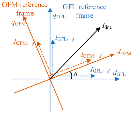
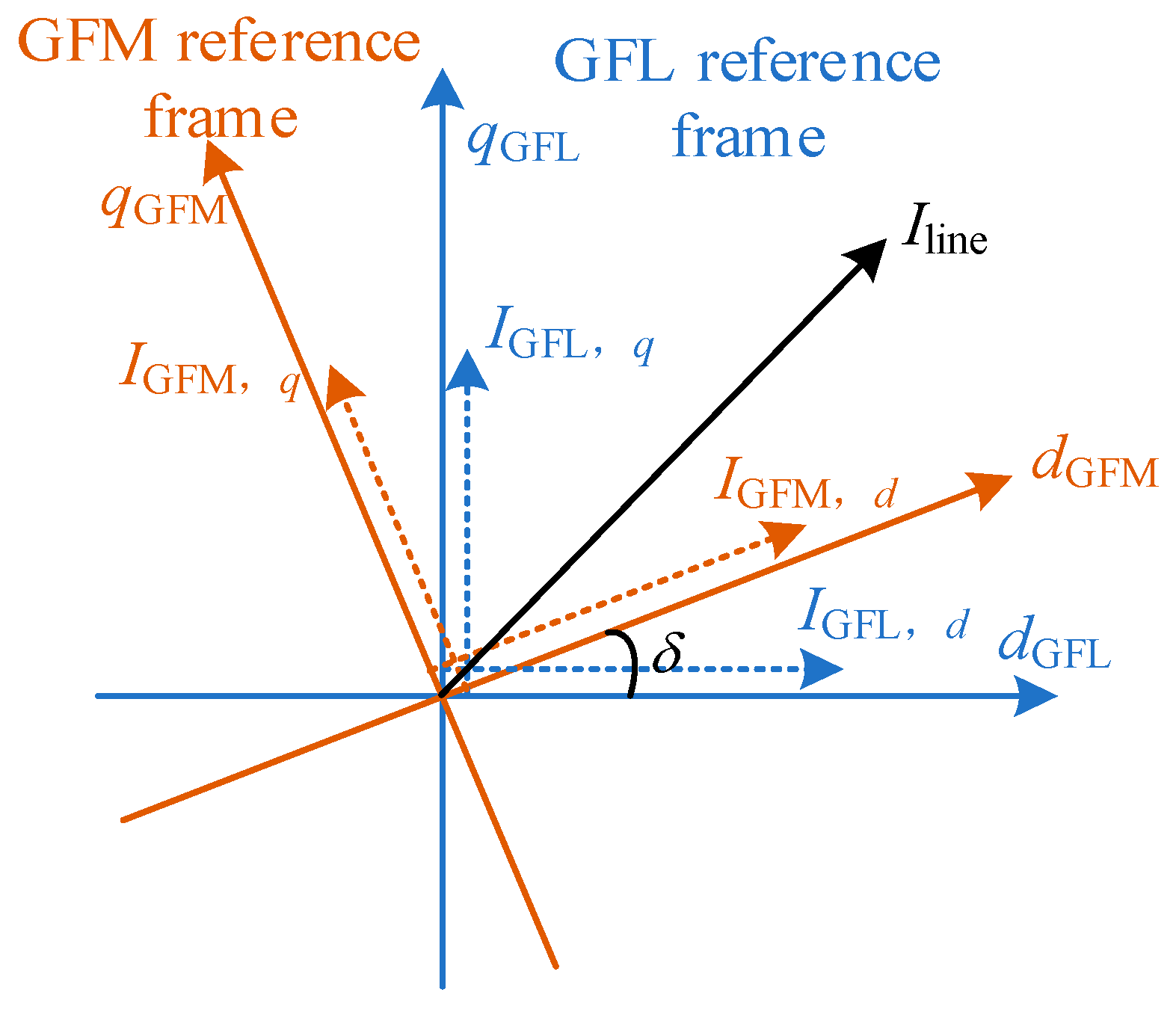
The decomposition of the current vector in the local and unified reference frames is illustrated in Figure 2.
Figure 2.
Vector mapping relationship of heterogeneous currents under multiple reference frames.
Because the GFL and GFM units employ independent phase references, their local reference frames exhibit significant deviations during the fault transient. Consequently, the line current contributed by different converter units cannot be directly superimposed or quantitatively analyzed in their respective local reference frames. To address this issue, a dynamic phase transformation is introduced to map the heterogeneous current components into the unified global synchronous reference frame. This enables vector synthesis of the multi-source currents and provides an accurate basis for calculating the transient equivalent impedance.
For GFL units, the phase-tracking process is described by Equation (10):
where denotes the internal phase angle generated by the converter controller, and is the angular frequency. Since is dynamically estimated by the PLL, its transient evolution during a fault follows a typical second-order dynamic response [27,28], which can be expressed as:
where denotes the pre-fault phase angle; is the phase-angle deviation; is the damping ratio; represents the nominal angular frequency; and is the damped oscillation frequency.
Equation (11) indicates that the phase angle is jointly determined by the PCC voltage and the PLL parameters during the fault transient, and therefore exhibits an oscillatory behavior. Once the PLL loses synchronization with the PCC voltage, the phase angle becomes highly uncertain.
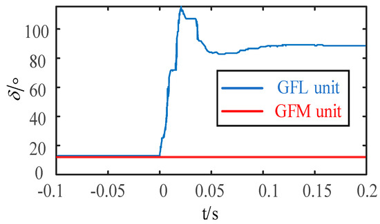
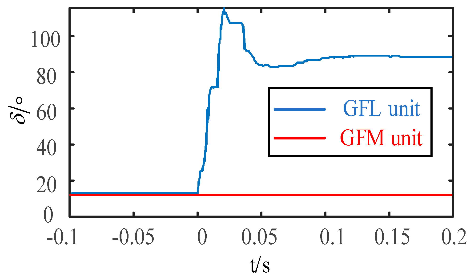
Unlike GFL units, the transient phase-angle dynamics of GFM units are primarily governed by the virtual damping coefficient and virtual inertia embedded in their control loops. During the fault transient, both the magnitude and the rate of change of the GFM output phase angle are significantly smaller than those of GFL units, and no high-frequency oscillations are observed. As illustrated in Figure 3, the power-angle variation of the GFM station remains within a limited range following the fault, indicating superior transient synchronization stability.
Figure 3.
Comparison of unit power angle under two control modes during failure.
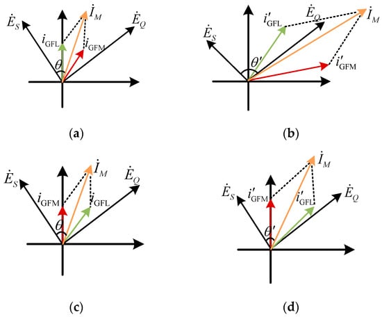
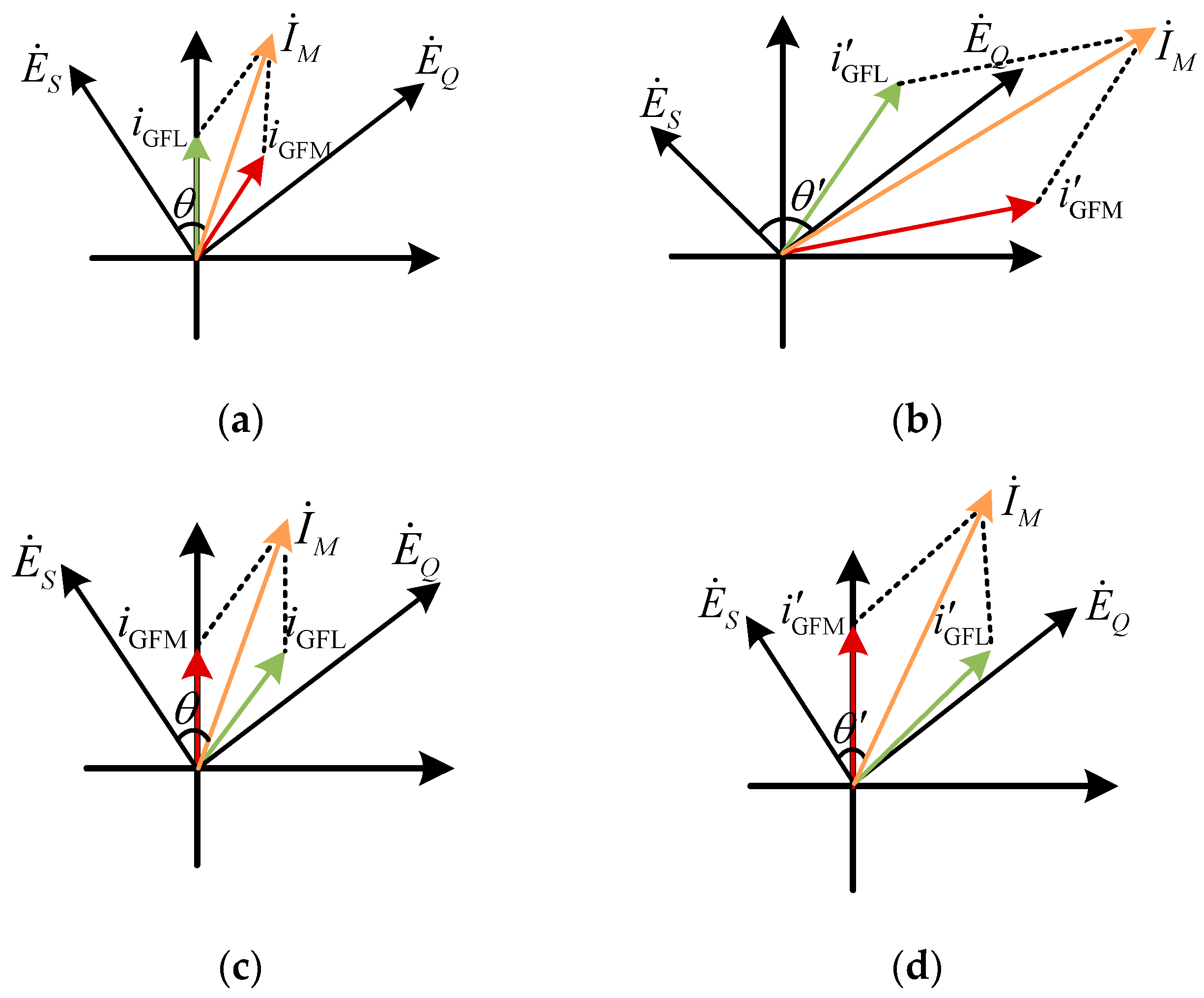
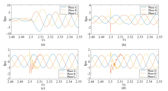
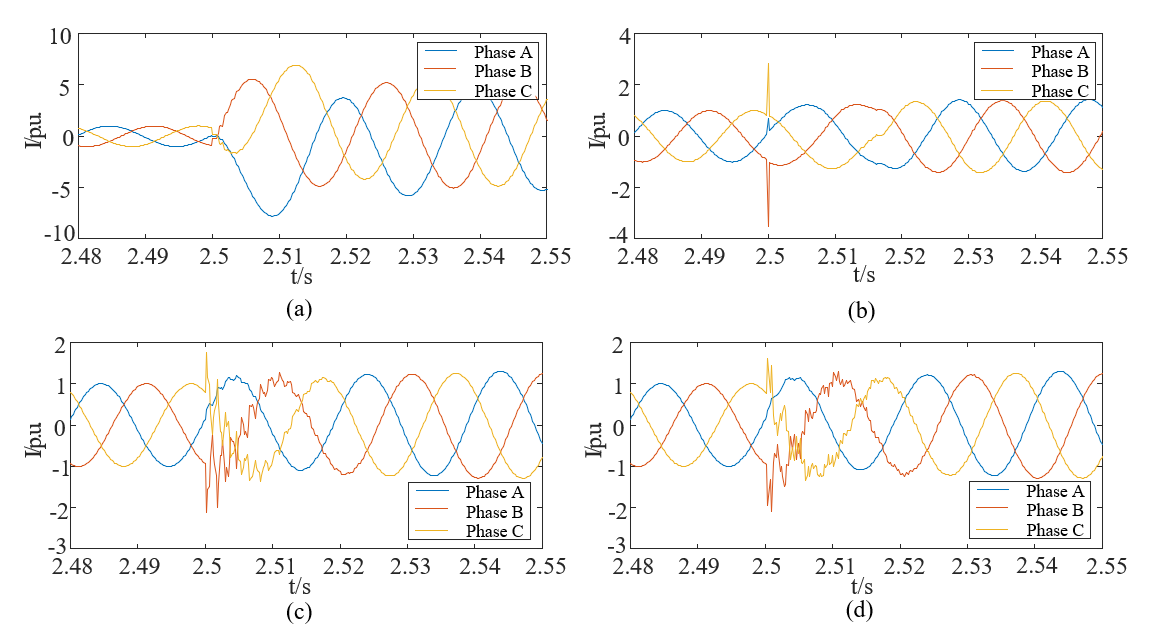
As illustrated in Figure 4a, under normal operating conditions, the PLL of the GFL unit accurately tracks the grid voltage, maintaining a stable phase relationship between the current vectors and the bus voltage. Consequently, the resultant line current exhibits a stable phase characteristic. However, as shown in Figure 4b, a short-circuit fault causes a voltage sag accompanied by an abrupt phase variation. The transient loss of synchronization of the GFL PLL results in severe oscillations of the output current phase. By contrast, as illustrated in Figure 4c,d, when the reference frame is established based on the phase angle of the GFM unit, the grid-forming control provides continuous voltage support and power-angle synchronization during the fault transient. Consequently, although the line current phase still deviates following the fault, the phase variation is significantly reduced compared with that in the conventional reference frame.
Figure 4.
Characteristics of electrical quantities before and after the fault under different reference frames: (a) Pre-fault conventional reference frame; (b) Post-fault conventional reference frame; (c) Pre-fault GFM reference frame; (d) Post-fault GFM reference frame.
Given the superior transient stability of the GFM power angle compared with that of GFL units, the GFM phase angle is adopted as the global phase reference for the hybrid renewable energy system. This unified reference effectively eliminates the phase-reference inconsistency introduced by heterogeneous converter control strategies, thereby enabling consistent analysis and vector synthesis of the line currents. Accordingly, the phase angle is transformed with respect to the GFM phase angle , as shown in Equation (12):
where and denote the d-axis and q-axis current components of the GFL unit expressed in the GFM reference frame, respectively; and is the dynamic phase difference between the two converter types.
After transforming the current components of all renewable energy stations into the GFM reference frame, the d-axis and q-axis currents of the outgoing transmission line can be obtained by the vector summation of the corresponding current components, as shown in Equation (13):
3.2. Definition of Transient Impedance
Conventional distance protection is established on the concept of the power-frequency steady-state impedance, defined as , where the operating voltage, , is used to characterize the electrical distance. Specifically, where the setting impedance is typically selected as 80–85% of the total transmission-line impedance.
However, under transient conditions, the voltage–current relationship of the transmission line is governed by the differential equations of the line R-L model rather than the steady-state impedance equation. After transforming the measured current into the d-q reference frame through the Park transformation and expressing all current components in the unified reference frame, the voltage–current relationship between the relay location and the protection setting boundary can be expressed in Equation (14):
where and denote the d-axis and q-axis voltage differences between the relay location and the protection setting boundary, respectively; and and represent the equivalent resistance and inductance corresponding to the protection setting boundary, respectively.
The transient equivalent impedance of the transmission line, denoted by , is defined as the ratio of the instantaneous voltage difference to the corresponding current, as shown in Equation (15):
Substituting (14) into (15) yields
where and are the d-axis and q-axis voltage components measured at the relay location, respectively; and are the corresponding voltage components at the protection setting boundary; and denotes the time-varying transient additional impedance.
To further investigate the variation mechanism of the transient additional impedance , the complex current phasor in the d-q reference frame is given by Equation (17):
where is the current magnitude, is the current phase angle, and denotes the complex conjugate of the current phasor. Substituting the above expression into (16) gives the result as shown in Equation (18):
As indicated by (17), the transient additional impedance consists of an additional resistive component and an additional reactive component, which are governed by the rate of change of the current magnitude and the phase-angle variation, respectively. Therefore, the transient equivalent impedance, , comprises not only the steady-state setting impedance, , but also a time-varying additional impedance, , introduced by the dynamic control behavior of renewable energy stations.
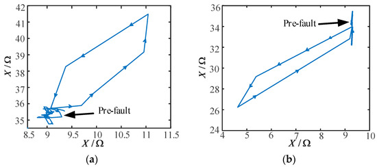
During the initial stage of an internal fault, the rapid increase in the current magnitude produces a positive shift in the additional resistive component, while the rotation of the current phase angle introduces an additional reactive component. The combined effect causes the transient impedance trajectory to deviate from the steady-state setting impedance. In contrast, for reverse external faults, the rotation direction of the fault-current phase angle is opposite to that of internal faults under the current reference direction and the unified reference frame adopted in this paper. Consequently, the polarity of the additional reactive component is reversed, causing the transient impedance trajectory to shift toward a different region of the impedance plane. These observations indicate that the evolution of the transient impedance inherently contains information on both the fault direction and the fault location. The corresponding transient impedance trajectories are illustrated in Figure 5.
Figure 5.
Evolution of transient impedance trajectories under faults both within and outside the region: (a) Transient impedance trajectory for an internal fault; (b) Transient impedance trajectory for a reverse external fault.
3.3. A Novel Distance Protection Scheme Based on Function Fitting
As demonstrated in Section 3.2, the transient impedance exhibits pronounced time-varying nonlinear characteristics, making it difficult to accurately identify faults using instantaneous impedance measurements alone. Prior to the fault, can be regarded as the protection setting impedance, whereas the transient additional impedance, , generated after fault inception reflects the characteristics of the fault location and protection zone. Therefore, to quantitatively establish the relationship between the transient impedance and the fault distance, the least-squares method is employed to fit the transient impedance with a linear function. The fitted function captures the overall evolution trend of the transient impedance and serves as the basis for constructing the proposed distance protection criterion.
Let denote the fault inception instant. Within a short data window immediately following the fault, n sampling instants are selected as in Equation (19):
where denotes the sampling instant with respect to the fault inception instant, and is the corresponding magnitude of the transient equivalent impedance. Since the transient impedance magnitude varies continuously within the short post-fault data window, it can be approximated by a first-order linear function.
where is the fitted function, is the fitted slope, and is the fitted intercept. To obtain the optimal fitting result, the objective function is defined as the sum of squared residuals.
According to the least-squares criterion, the fitting parameters and satisfy Equation (22):
By setting the partial derivatives of the objective function with respect to and equal to zero, the resulting expressions are obtained, as shown in Equation (23):
where and denote the mean values of the sampling-time sequence and the transient impedance magnitude sequence , respectively, as shown in Equation (24):
Accordingly, the linear fitting function of the transient impedance magnitude over the short post-fault data window can be expressed as in Equation (25):
Further examination of (25) shows that the numerator of the slope is determined by the covariance between the sampling time and the transient impedance magnitude , whereas the denominator represents the discrete variance of the sampling time. Therefore, characterizes the average rate of change of the transient impedance magnitude with respect to time. When the transient impedance magnitude increases over the post-fault data window, ; conversely, when it decreases. A larger absolute value of indicates a more pronounced variation in the transient impedance trajectory. Accordingly, the slope can be employed to characterize both the direction and the rate of evolution of the transient impedance trajectory.
The intercept represents the initial offset of the transient impedance magnitude from the protection setting impedance immediately after fault inception. Under normal operating conditions, or when the transient additional impedance is negligible, approaches the magnitude of the protection setting impedance. Following a fault, however, the transient impedance is influenced by the fault location, fault direction, and the transient control dynamics of renewable energy stations, resulting in a corresponding shift of . Therefore, the intercept b provides an effective indicator of the initial position of the transient impedance trajectory.
The above analysis indicates that faults occurring at different locations produce distinct transient electrical responses in terms of both magnitude and dynamic variation. The proposed fitting parameters, namely the slope and the intercept , effectively capture these characteristics. Consequently, fault location and fault direction can be discriminated using the fitted linear function. Let denote the slope obtained under normal operating conditions, which is approximately zero, and let denote the corresponding intercept, whose value is approximately equal to the magnitude of the line setting impedance.
Since the intercept reflects the relative position of the fault, the difference ( − ) is adopted to distinguish forward and reverse faults. Meanwhile, the slope is primarily determined by the transient process and exhibits a clear dependence on the fault distance. Accordingly, the proposed protection criterion is given by Equation (26):
where is the fitted slope obtained under normal operating conditions, which is typically close to zero; is the magnitude of the protection setting impedance, generally selected as 80–85% of the transmission-line impedance, and is set to 85% in this paper; and are the slope and intercept obtained in real time from the fitted function using the measured data.
Since a three-phase short-circuit fault produces the most severe transient response and the most pronounced electrical characteristics, the fitted slope obtained under an internal three-phase fault is adopted as the lower reference limit for setting the proposed protection criterion. To achieve a balance between protection sensitivity and tolerance to transition resistance, the fitted slope corresponding to a three-phase-to-ground fault with a transition resistance of 50 Ω is selected as the protection threshold. This setting strategy accounts for the attenuation of transient characteristics under high-resistance faults, thereby enhancing the operating reliability of the proposed protection scheme, as shown in Equation (27):
where denotes the reliability coefficient, which is set to 0.95 in this paper, and is the fitted slope obtained when a three-phase-to-ground fault with a transition resistance of 50 Ω occurs at the remote end of the protected line.
The proposed protection criterion is established from the transient evolution of the impedance rather than its steady-state value. Moreover, the dynamic phase transformation requires only the d- and q-axis components and does not rely on the data window required for Fourier-based algorithms. Consequently, the overall operating time of the protection scheme is less than 15 ms.
To more intuitively illustrate the discrimination logic of the fitting parameters under different fault scenarios, Table 2 summarizes the classification rules for internal/external faults based on the combined criterion of a and b.
Table 2.
Internal/external fault discrimination logic based on fitting parameters.
Here, a0 is the reference value of the fitting slope under normal operating conditions (approximately zero), b0 is the reference value of the fitting intercept under normal operating conditions (corresponding to the setting impedance), and aset is the slope threshold set based on the three-phase fault at the end of the protected zone (a negative value). The above criterion indicates that the protection identifies an internal fault only when a lies between aset and a0 and the deviation direction of b is consistent with the internal fault characteristics; otherwise, it identifies an external fault and issues a block signal.
3.4. Protection Procedure
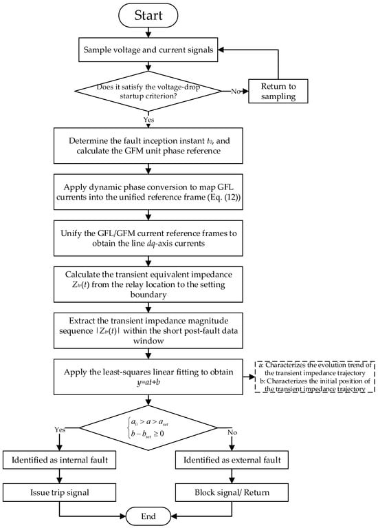
The overall procedure of the proposed protection scheme is illustrated in Figure 6. Following fault inception, the protection algorithm is activated once the voltage-sag criterion is satisfied. Based on the known control parameters of the GFM unit, its output current phase angle is first calculated. Subsequently, the output current of the GFL unit is transformed into the unified reference frame using the proposed dynamic phase transformation, thereby achieving phase synchronization of the output currents from the hybrid renewable energy station.
Figure 6.
Protection Discrimination Process.
The transient equivalent impedance between the relay location and the protection setting boundary is then calculated, and the transient impedance magnitude sequence within a short post-fault data window is extracted. A least-squares linear fitting is subsequently performed on the impedance magnitude sequence to obtain its first-order time-domain fitting function. Finally, the fitted slope and intercept are compared with the preset protection thresholds to identify the fault location and determine the corresponding protection action.
4. Simulation Verification
To validate the effectiveness of the proposed distance protection scheme, a hybrid renewable energy integration system, as illustrated in Figure 1, was established in the PSCAD/EMTDC simulation environment. Comprehensive case studies were conducted to evaluate the proposed method under different fault locations, fault types, renewable power outputs, and transition resistances.
The rated capacities of both the GFL and GFM renewable energy stations were set to 100 MW. The outgoing transmission line operates at 220 kV with a total length of 100 km. The detailed parameters of the transmission line, the main transformer, and the renewable energy stations are summarized in Table 3.
Table 3.
Simulation Model Parameters.
Five fault locations were considered, including the renewable-station terminal, points located 25 km, 50 km, and 75 km from the renewable-station side, and the grid-side terminal, denoted as , respectively. Unless otherwise specified, all faults were applied at 2.5 s.
According to the transmission-line parameters and the setting procedure described in Section 3, the magnitude of the protection setting impedance is determined as . Under normal operating conditions, the fitted slope is obtained as . Using the three-phase fault at the remote end of the protected line as the reference condition, the fitted slope is , yielding a theoretical protection threshold of . To account for model parameter uncertainties and operating-condition variations, the protection threshold is finally set to .
4.1. Validation of the Transient Current Phase Transformation
The transient current characteristics under different fault locations are illustrated in Figure 7. When a three-phase-to-ground fault occurs at F1, which is located behind the relay, the measured current is dominated by the fault current supplied by the strong grid on the opposite side, resulting in a relatively large transient current magnitude. For forward faults, the transient current magnitude gradually decreases as the fault location moves farther away from the relay. These results confirm that the fault distance has a significant influence on the transient current magnitude, which is consistent with the theoretical analysis presented in Section 3.
Figure 7.
Transient currents at different fault locations: (a) Transient current for fault at F1; (b) Transient current for fault at F2; (c) Transient current for fault at F3; (d) Transient current for fault at F4.
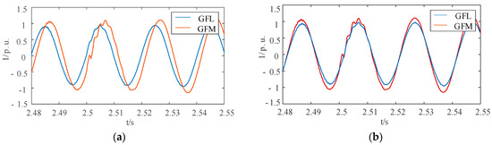
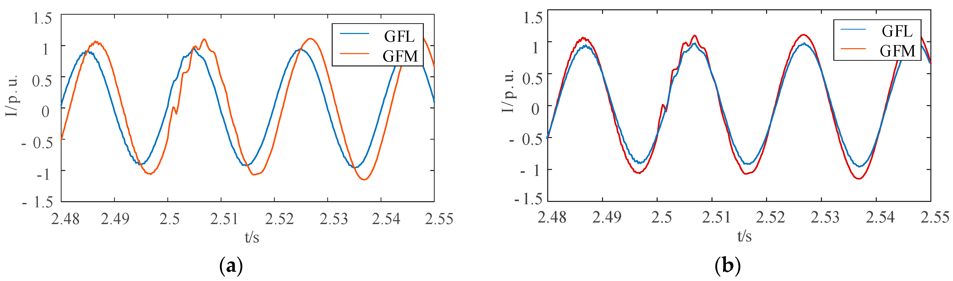
Figure 7 demonstrates that different fault locations produce distinct transient current magnitudes, indicating that the current magnitude can serve as an auxiliary feature for fault-zone discrimination. Figure 8 further compares the phase-A current waveforms before and after the proposed phase transformation, together with the phase-angle difference between the GFL and GFM units. As shown in Figure 8a, a pronounced phase mismatch exists between the output currents of the GFL and GFM units before the phase transformation. Consequently, both the zero-crossing instants and the current peaks are significantly misaligned, and their direct superposition results in severe phase distortion of the transmission-line current. After transforming the GFL current into the unified reference frame using the GFM phase as the reference, the output currents of the two converter types become well aligned, as illustrated in Figure 8b.
Figure 8.
Results of dynamic current phase conversion after a fault: (a) Current under AG fault before phase conversion; (b) Current under AG fault after phase conversion.
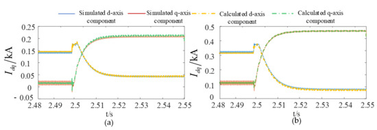
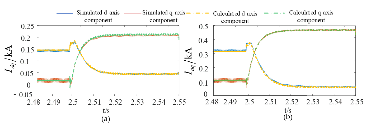
Figure 9 compares the simulated and analytical d-axis currents of the GFL unit before and after the proposed phase transformation. According to the LVRT control strategy and the system parameters, the theoretical steady-state values of the d-axis current after fault inception are 52.5 A and 210.62 A, respectively. As shown in Figure 9a, the electromagnetic transient simulation agrees closely with the analytical solution, thereby validating the accuracy of the proposed transient current analytical model.
Figure 9.
Calculation values of the dq-axis components before and after conversion versus simulation waveforms: (a) Before phase conversion; (b) After phase conversion.
Figure 9b further presents the d-axis current expressed in the unified reference frame. A noticeable difference can be observed between the current waveforms before and after the phase transformation, demonstrating that the proposed dynamic phase transformation is essential for accurately representing the output current of the hybrid renewable energy station during transient conditions.
The above results demonstrate that the proposed phase conversion method can effectively unify the reference frames of heterogeneous currents, providing a reliable basis for accurate calculation of the transient equivalent impedance. On this basis, the correctness of the proposed impedance fitting criterion under different fault types and locations needs to be further verified.
4.2. Influence of Fault Location and Fault Type on Protection Performance
Since different fault types may occur at different locations along the outgoing transmission line, simulations were conducted to evaluate the adaptability of the proposed protection scheme under various operating conditions. Accordingly, different fault types were applied at each predefined fault location, and the corresponding protection performance is summarized in Table 4.
Table 4.
Protection actions for different fault locations and types.
From Table 4, the following patterns can be observed. Horizontally, at the same fault location, more severe fault types (ABCG > BCG > BC > AG) yield larger values of |a|, indicating that the transient impedance variation becomes more intense as the fault severity increases, which is consistent with the physical characteristics of fault currents. Vertically, for the same fault type, both |a| and b increase monotonically with fault distance (F2 → F3 → F4), suggesting that both the initial position and the variation magnitude of the transient impedance are positively correlated with the fault distance. In contrast, external faults exhibit distinct characteristics that clearly distinguish them from internal faults. For the reverse external fault F1, a is positive and b is negative, providing additional information for identifying the fault direction. For the forward external fault F5, although the slope a may appear to satisfy the internal condition, the intercept b is significantly larger than the range observed for internal faults, thereby enabling reliable blocking through the b-based auxiliary criterion. For internal faults, the proposed criterion operates correctly even when the fault is located near the boundary of the protected line. These results demonstrate the robustness of the proposed protection scheme under different fault locations and fault types, and confirm the effectiveness of the combined criterion using both a and b.
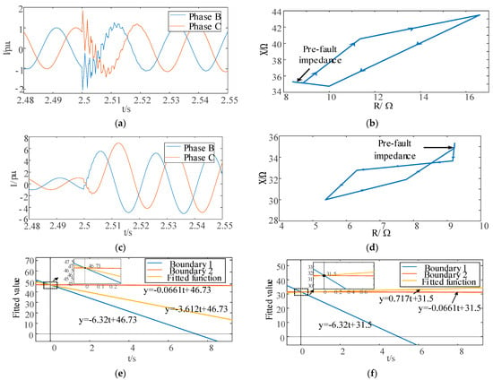
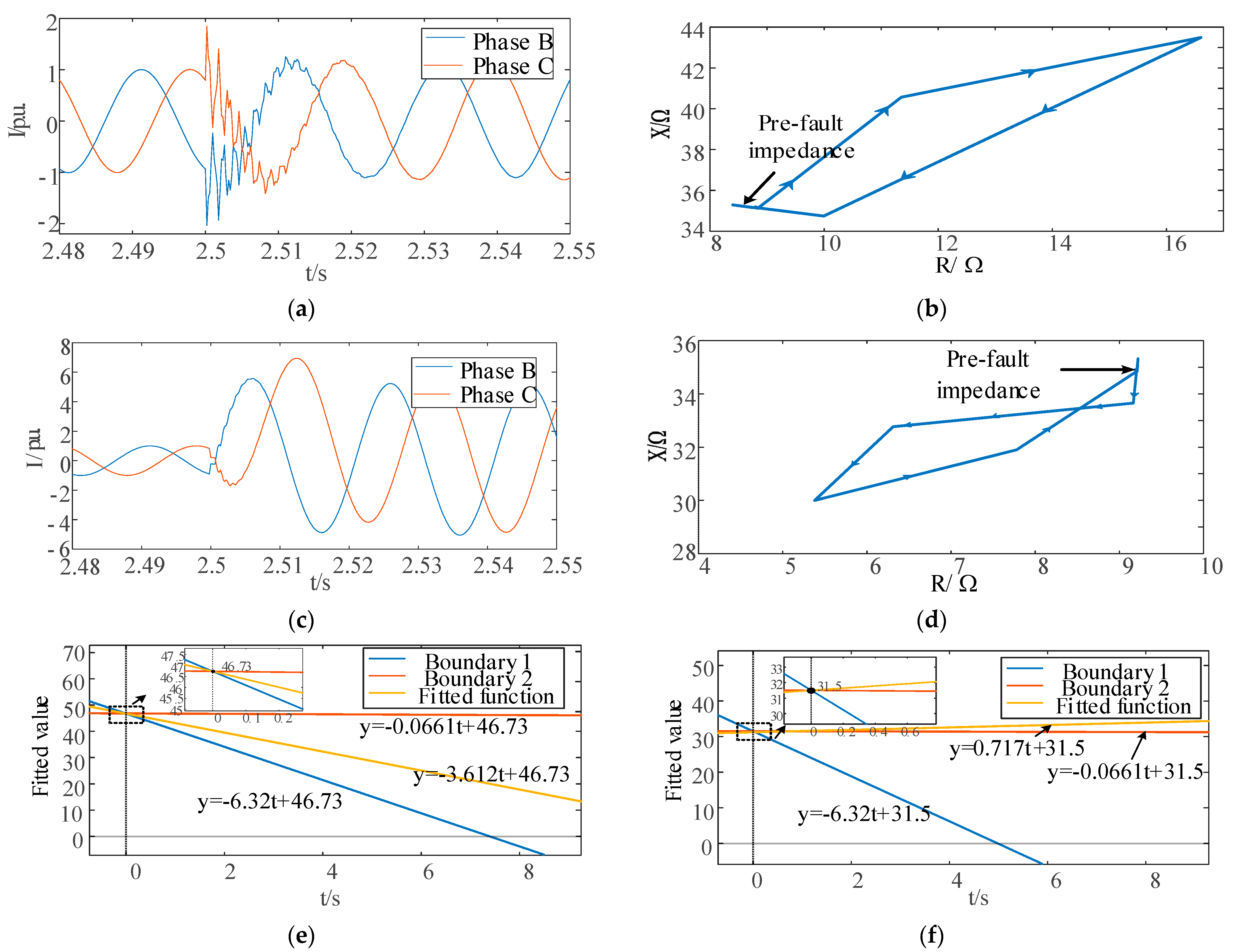
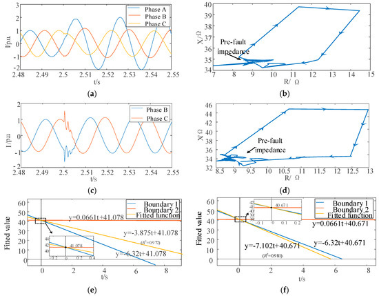
To further illustrate the operating characteristics of the proposed criterion, a BC phase-to-phase fault at the internal fault location F3 and a BCG phase-to-ground fault at the external fault location F1 were selected as representative cases. The corresponding transient responses are presented in Figure 10. As shown in Figure 10a,c, the measured current magnitude decreases as the fault location moves farther away from the relay, accompanied by a reduction in the transient response intensity. The transient impedance trajectories shown in Figure 10b,d are consistent with the theoretical analysis presented in Section 3, exhibiting distinct evolution patterns for internal and external faults.
Figure 10.
Protection components under different fault types within and outside the region: (a) Current waveforms under fault at F3; (b) Transient impedance trajectory under BC fault at F3; (c) Current waveforms under fault at F1; (d) Transient impedance trajectory under BC fault at F1; (e) Fitted function and operating boundary under BC fault at F3; (f) Fitted function and operating boundary under BC fault at F1.
The protection decision process is illustrated in Figure 10e,f. The fitted linear functions constructed from the slope a and intercept b satisfy the operating criterion for the internal fault, whereas the external fault satisfies the blocking criterion, confirming the effectiveness of the proposed method in discriminating different fault locations and fault types. It should be noted that the horizontal axis in Figure 10e,f does not represent the actual fault duration. Instead, it is a sequential time axis introduced to visualize the relationship between the fitted parameters and the corresponding protection thresholds. The protection decision is completed within 15 ms in all cases. The same representation is adopted in the following figures.
Although the proposed method performs well under metallic faults, the presence of transition resistance in practical systems often causes conventional protection to fail. Therefore, it is necessary to further assess the tolerance of the method under high-resistance faults.
4.3. Performance Under Different Transition Resistances
Transition resistance is one of the primary factors affecting the reliability of transmission-line protection and is particularly challenging for conventional distance protection. To evaluate the tolerance of the proposed protection scheme to transition resistance, simulations were carried out under different fault locations, fault types, and transition resistance conditions. The corresponding protection results are summarized in Table 5.
Table 5.
Protection operation under different transition resistance conditions.
As shown in Table 5, the proposed criterion correctly identifies the fault zone and operates reliably under all tested transition resistance conditions. Although the fitted slope decreases with increasing transition resistance, its variation remains strongly correlated with the relative distance between the fault location and the relay. For phase-to-phase faults, the proposed protection continues to operate correctly even in the presence of relatively large transition resistances, demonstrating strong robustness against transition resistance. These results indicate that the proposed scheme effectively mitigates the adverse influence of transition resistance on conventional distance protection.
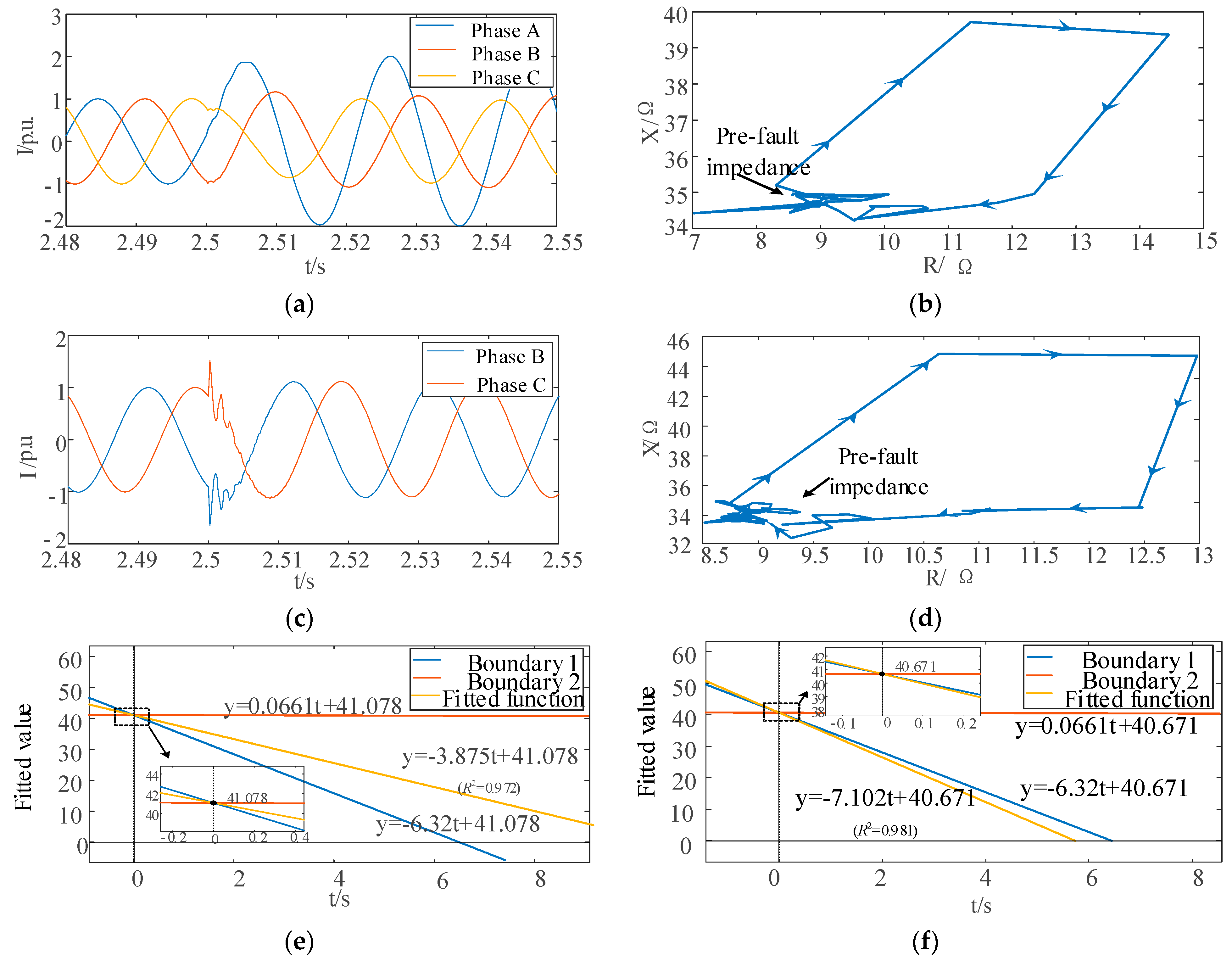
To further illustrate the protection performance, representative cases involving faults at F3 and F5 under different transition resistances are presented in Figure 11. As shown in Figure 11a,c, the measured current magnitude decreases as the fault location moves farther away from the relay, accompanied by a weaker transient response. The transient impedance trajectories shown in Figure 11b,d remain nearly constant before fault inception and exhibit regular variations after the fault owing to the transient additional impedance. Even in the presence of transition resistance, the transient impedance increases with increasing fault distance, which is consistent with the theoretical analysis presented in Section 3.
Figure 11.
Protection components under different fault types caused by varying transition impedances within and outside the region: (a) Current waveforms under AG fault at F3 with 100 Ω transition resistance; (b) Transient impedance trajectory under AG fault at F3 with 100 Ω transition resistance; (c) Current waveforms under BC fault at F5 with 200 Ω transition resistance; (d) Transient impedance trajectory under BC fault at F5 with 200 Ω transition resistance; (e) Fitted function and operating boundary under AG fault at F3; (f) Fitted function and operating boundary under BC fault at F5.
The corresponding fitting results are shown in Figure 11e,f. Taking the forward external fault at F5 as an example, the fitted slope is −7.102, which satisfies the blocking criterion and therefore does not trigger the protection. The results demonstrate that the proposed protection scheme correctly identifies the fault zone under a transition resistance of , indicating its excellent tolerance to transition resistance.
The transition resistance tests have validated the method’s tolerance capability. However, renewable power output varies significantly with environmental conditions, leading to substantial differences in fault current magnitudes. To comprehensively evaluate the engineering adaptability, the influence of power fluctuations must also be considered.
4.4. Protection Performance Under Different Renewable Power Outputs
The output power of renewable energy stations is highly dependent on environmental conditions. To evaluate the adaptability of the proposed protection scheme to power fluctuations, the output power of the renewable energy station was set to 25 MW, 50 MW and 100 MW, and the results were compared with those obtained under the rated operating condition. In the simulations, different types of internal faults were applied at F3, while a reverse three-phase-to-ground external fault was applied at F1. The corresponding protection results are summarized in Table 6.
Table 6.
Protection actions under different output conditions of the station.
As shown in Table 6, the proposed criterion operates correctly for both internal and external faults when the renewable power output is reduced from the rated value to 50 MW and 25 MW. These results demonstrate that the proposed transient impedance fitting-based protection method exhibits strong adaptability to renewable power fluctuations and maintains reliable fault-zone discrimination over a wide range of operating conditions.
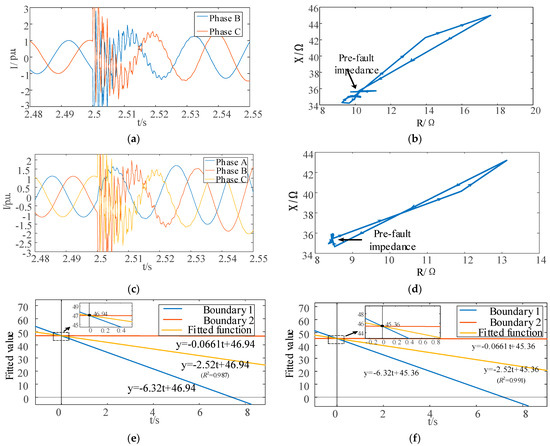
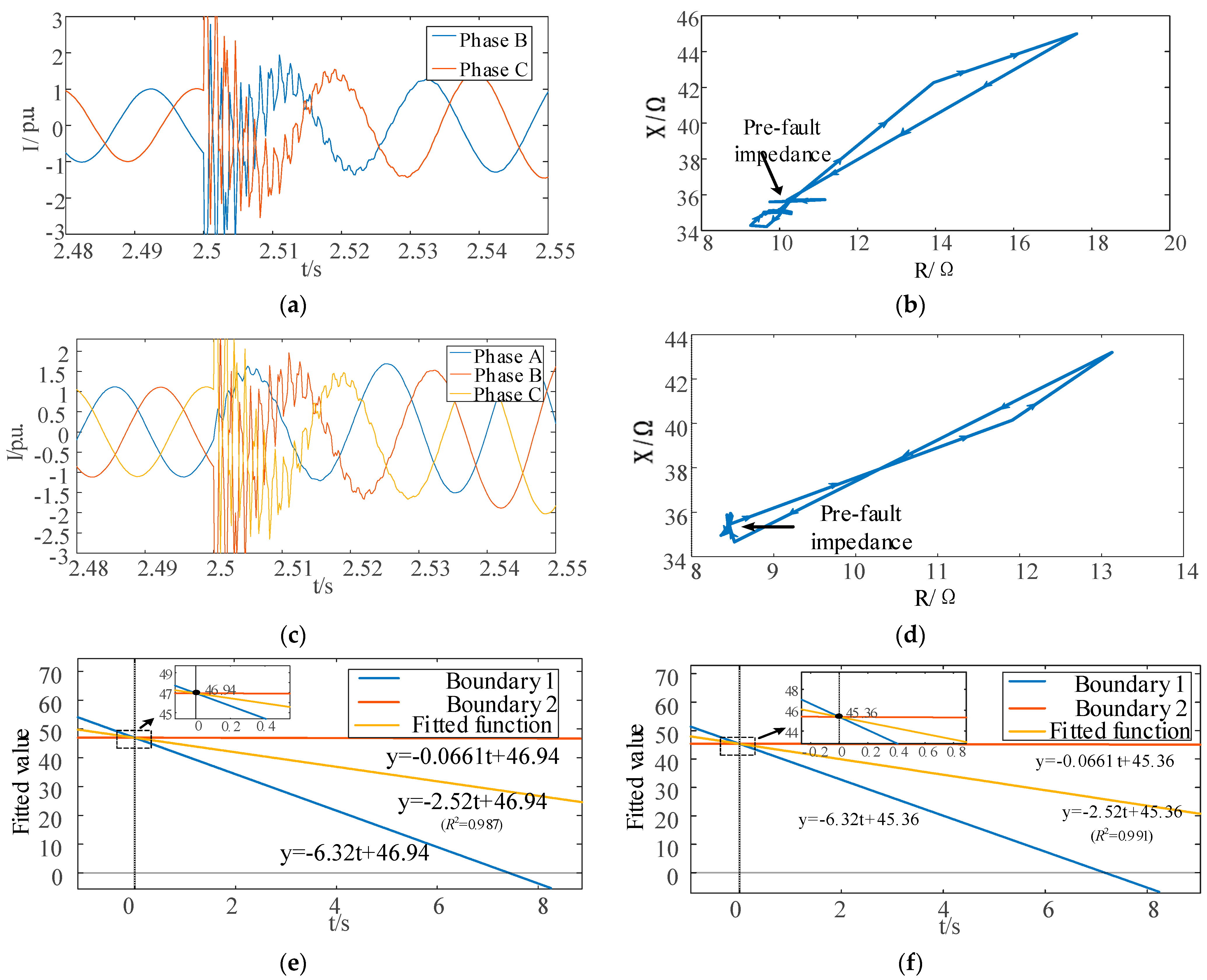
The transient responses under different renewable power outputs are illustrated in Figure 12. For the BC phase-to-phase fault and the ABCG four-phase-to-ground fault at F3, the transient fault current varies with the renewable power output. Nevertheless, the transient impedance trajectory consistently retains the characteristic behavior of an internal fault. As shown in Figure 12e,f, the fitted slope satisfies the operating criterion for internal faults, while the fitted intercept remains within the reliable operating range. These results further confirm that the proposed protection scheme accurately identifies internal faults under varying renewable power outputs, demonstrating excellent adaptability to changing operating conditions.
Figure 12.
Protection components under different fault types occurring at varying station output levels: (a) Current waveforms under BC fault at F3 with 25 MW output power; (b) Transient impedance trajectory under BC fault at F3 with 25 MW output power; (c) Current waveforms under ABCG fault at F3 with 50 MW output power; (d) Transient impedance trajectory under ABCG fault at F3 with 50 MW output power; (e) Fitted function and operating boundary under BC fault with 25 MW output power; (f) Fitted function and operating boundary under ABCG fault with 25 MW output power.
4.5. Performance Comparison with Conventional Methods
To demonstrate the performance improvement quantitatively, the proposed method is compared with conventional positive-sequence voltage polarized phase-comparison distance protection under identical simulation conditions.
The correct discrimination rates of the two methods under different fault scenarios are summarized in Table 7. The test cases cover metallic faults, high-resistance faults with transition resistances of 50 Ω, 100 Ω, and 200 Ω, and low-output conditions of 50 MW and 25 MW.
Table 7.
Comparison of correct discrimination rates between conventional and proposed methods.
As shown in Table 7, conventional distance protection achieves acceptable performance under metallic faults, with a correct rate of 83.3%. However, its performance degrades significantly as the transition resistance increases. When the transition resistance reaches 200 Ω, the correct discrimination rate drops to 66.7%. Under low-output weak-infeed conditions (25 MW), the correct rate further decreases to 60.0%. The primary reason is that conventional distance protection relies on steady-state fundamental-frequency impedance measurements, which are highly susceptible to additional impedance deviation caused by fault resistance and inverter control dynamics. In contrast, the proposed method maintains 100% correct discrimination across all 49 test cases, demonstrating significantly stronger robustness against high-resistance faults and weak-infeed conditions.
The operating speed of the two methods is compared in Table 8. The proposed method utilizes only 10 ms of post-fault data (half a power-frequency cycle), whereas conventional Fourier-based phasor estimation requires at least one full cycle (20 ms) to establish steady-state phasors.
Table 8.
Comparison of typical operating time.
As shown in Table 8, the proposed method completes fault discrimination within 15 ms, achieving a speed advantage of at least 5–25 ms over conventional distance protection. This speed advantage is particularly beneficial for renewable-integrated transmission systems, where fault current characteristics are highly transient and fast fault clearance is essential for maintaining system stability.
5. Conclusions
This paper proposes a transient impedance fitting-based distance protection scheme to address the degraded adaptability of conventional distance protection in power systems with high penetration of renewable energy. By establishing a unified current reference frame for hybrid GFL/GFM renewable energy stations, a transient equivalent impedance model is developed, and the fitted parameters of the transient impedance magnitude are employed for fault-zone discrimination. The main conclusions are summarized as follows.
- A dynamic phase transformation method referenced to the GFM phase angle is proposed to eliminate the inconsistency of transient current phase references between GFL and GFM renewable energy stations. The proposed method enables the synthesis of heterogeneous converter currents in a unified reference frame, providing the foundation for accurate calculation of the transient equivalent impedance.
- Based on the unified reference frame, a transient equivalent impedance model incorporating transient additional impedance is established. A least-squares linear fitting is then applied to extract the dynamic characteristics of the transient impedance magnitude. The fitted slope and intercept respectively characterize the evolution trend and the initial position of the transient impedance trajectory, enabling reliable discrimination between internal and external faults while reducing the dependence of conventional distance protection on steady-state fundamental-frequency impedance.
- Simulation results demonstrate that the proposed protection scheme accurately identifies fault zones under various fault locations, fault types, transition resistances, and renewable power output conditions. The proposed method exhibits fast operating speed, high selectivity, and strong reliability, thereby effectively mitigating the maloperation and failure-to-operate issues encountered by conventional distance protection in renewable-rich power systems.
Author Contributions
Conceptualization, Z.L. and G.Y.; methodology, Z.L. and D.C.; validation, D.C. and J.Q.; formal analysis, Z.L., G.Y. and D.C.; investigation, X.F.; resources, Z.L.; data curation, D.C. and J.Q.; writing—original draft preparation, D.C., G.Y. and J.Q.; writing—review and editing, D.C. and X.F.; visualization, J.Q.; supervision, Z.L. All authors have read and agreed to the published version of the manuscript.
Funding
This research received no external funding.
Data Availability Statement
Data supporting the reported results are available from the corresponding author upon reasonable request.
Conflicts of Interest
Author Guang Yang was employed by State Grid Electric Lichuan Power Supply Company. The remaining authors declare that the research was conducted in the absence of any commercial or financial relationships that could be construed as a potential conflict of interest.
References
- Nurunnabi, M.; Li, S. Protection in Inverter-Dominated Grids: Fault Behavior of Grid-Following vs. Grid-Forming Inverters and Mixed Architectures—A Review. Energies 2026, 19, 684. [Google Scholar] [CrossRef] [Scilit]
- Li, Y.; Wu, H.; Wang, X. Challenges for Distance Relays in Grid Code-Compliant Inverter-Based Power Systems: A Review. IEEE Open J. Power Electron. 2025, 7, 128–145. [Google Scholar] [CrossRef] [Scilit]
- Hasan, M.M.; Razmi, D.; Babayomi, O.; Davidson, I.; Terzija, V.; Zhang, Z. Advanced control and protection strategies for grid-forming inverters in microgrids—A review. Int. J. Electr. Power Energy Syst. 2025, 172, 111297. [Google Scholar] [CrossRef] [Scilit]
- Li, Y.; Yuan, X.; He, W.; Liu, W. Causal Relationships Among Electrical Quantities in Grid-Connected Inverter Systems Following Short-Circuit Faults Based on Device and Network Excitation–Response Mechanisms. In Proceedings of the 2025 6th International Conference on Electrical Technology and Automatic Control (ICETAC), Nanjing, China, 20–22 June 2025; pp. 478–487. [Google Scholar] [CrossRef] [Scilit]
- Kunwar, D.R.; Hossain, S.M.; Gujar, A. Analytical Study of the Transient Period of Fault Current in Inverter-Based Resources. In Proceedings of the 2024 IEEE Third International Conference on Power Electronics, Intelligent Control and Energy Systems (ICPEICES), Delhi, India, 26–28 April 2024; pp. 808–813. [Google Scholar] [CrossRef] [Scilit]
- Li, G.; Zhang, Z.; Zhao, R.; Xu, B. Fault characteristics and protection methods for long distribution lines with grid-forming IBDG integration. Electr. Power Syst. Res. 2024, 241, 111274. [Google Scholar] [CrossRef] [Scilit]
- Loebel, J.; Jaeger, J. Analytical investigation of influence of grid following IBR control on distance protection. In Proceedings of the 19th IET Conference on Developments in Power System Protection (DPSP Europe 2025), Bilbao, Spain, 1–3 April 2025; pp. 147–154. [Google Scholar] [CrossRef] [Scilit]
- George, N.; Naidu, O.D.; Pradhan, A.K. Distance Protection for Lines Connecting Converter Interfaced Renewable Power Plants: Adaptive to Grid-end Structural Changes. IEEE Trans. Power Deliv. 2023, 38, 2011–2021. [Google Scholar] [CrossRef] [Scilit]
- Daryabar, H.; Abedini, M.; Davarpanah, M. An adaptive K-factor control scheme for inverter-based resources to enhance operation of distance protection. Int. J. Electr. Power Energy Syst. 2025, 173, 111349. [Google Scholar] [CrossRef] [Scilit]
- Li, B.; Mu, R.; He, J.; Wang, W.; Yao, C.; Zhang, Y. Transient Fault Current Calculation Method for the PV Grid-Connected System Considering Dynamic Response of PLL. IEEE Trans. Ind. Appl. 2024, 60, 7537–7547. [Google Scholar] [CrossRef] [Scilit]
- Ordono, A.; Sanchez-Ruiz, A.; Zubiaga, M.; Asensio, F.J.; Cortajarena, J.A. Current limiting strategies for grid forming inverters under low voltage ride through. Renew. Sustain. Energy Rev. 2024, 202, 114657. [Google Scholar] [CrossRef] [Scilit]
- Ren, B.; Wang, C.; Li, Q.; Zou, X.; Wang, D.; Hu, Y. An Oscillation Stability Analysis of a Direct-Driven Wind Power Grid-Connected System Considering Low Voltage Ride though from an Energy Perspective. Electronics 2024, 13, 3489. [Google Scholar] [CrossRef] [Scilit]
- Luo, J.; Liu, Y.; Cui, Q.; Zhong, J.; Zhang, L. Single-ended time domain fault location based on transient signal measurements of transmission lines. Prot. Control Mod. Power Syst. 2024, 9, 61–74. [Google Scholar] [CrossRef] [Scilit]
- Wang, Z.; Mu, L. Microgrid fault detection method coordinated with a sequence component current-based fault control strategy. Prot. Control Mod. Power Syst. 2024, 9, 81–93. [Google Scholar] [CrossRef] [Scilit]
- Li, Y.; Jia, N.; He, J.; Li, B.; Wang, H.; Zhang, S. Non-unit protection scheme based on cooperation with control strategy for multiterminal hybrid HVDC system without line boundary. Prot. Control Mod. Power Syst. 2025, 10, 41–55. [Google Scholar] [CrossRef] [Scilit]
- Wang, K.; Lin, X.; Wei, F.; Li, Z.; Gao, J.; Weng, H. Enhancing Superimposed-Based Distance Protection in Inverter-Dominated Grids Based on Control-Protection Coordination. IEEE Trans. Ind. Electron. 2026, 73, 2092–2103. [Google Scholar] [CrossRef] [Scilit]
- Gao, B.; Liu, P.; Sun, D.; Wang, X.; Wu, L.; Deng, P.; Zheng, Z.; Ju, M. Analysis of Subsynchronous Oscillation Characteristics and Mechanism of Grid-Forming/Grid-Following Hybrid Wind Farms. Trans. China Electrotech. Soc. 2025, 40, 1945–1959. [Google Scholar] [CrossRef]
- Wang, G.; Pei, W.; Xiong, J.; Li, Y.; Su, X. Review of Coordinated Control Strategies for Renewable Energy Station with Grid-following and Grid-forming Inverters. High Volt. Eng. 2025, 51, 793–805. [Google Scholar] [CrossRef]
- Xu, N.; Chu, X.; Ye, H. Active Power Coordination for a Large Population of Grid-Forming and Grid-Following Inverters Based on Mean Field Games Theory. IEEE Access 2023, 11, 90052–90064. [Google Scholar] [CrossRef] [Scilit]
- Yuan, S.; Ge, Z.; Tang, J.; Mei, J. Longitudinal Protection of Grid-Forming New Energy Outgoing Lines Based onComposite Sequence Current Characteristics. Electr. Power 2025, 58, 185–192. [Google Scholar] [CrossRef]
- Ríos-Castro, D.; Fernández-Abraldes, P.M.; Pérez-Estévez, D.; Doval-Gandoy, J. Grid-Forming Converter with Enhanced Current Limiting Dynamics During Grid Faults and Wide Stability Range. IEEE Trans. Power Electron. 2025, 40, 15042–15063. [Google Scholar] [CrossRef] [Scilit]
- Kuang, X.; Fang, Y.; Guan, H.; Li, J.; Jia, K.; Bi, T.S. Full-time domain short circuit current calculation method suitable for power network with inverter-interfaced renewable energy source. Electr. Power Autom. Equip. 2020, 40, 113–122. [Google Scholar] [CrossRef]
- Liu, H.; Wang, Y.; Liu, Y.; Peng, Y.; Li, M.; Lei, W. The LVRT Strategy for VSG Based on the Quantitatively Designed Virtual Impedance. High Volt. Eng. 2022, 48, 245–256. [Google Scholar] [CrossRef]
- Chao, C.; Zheng, X.; Gao, P.; Tai, N.; Jin, S.; Tu, Q. Adaptive Distance Protection for Transmission Line of Photovoltaic Station During Asymmetric Short Circuit. Proc. CSEE 2022, 42, 6681–6693. [Google Scholar] [CrossRef]
- Yang, G.; Wang, R.; Wang, C.; Yu, Y.; Lv, P. Distance Protection Principle for Renewable Energy Transmission Lines Based onNegative Sequence Suppression Strategy Characteristics. Power Syst. Technol. 2026, 50, 1719–1730. [Google Scholar] [CrossRef]
- Zhou, Z.; Yu, S.; Li, Y.; Wang, X. Analysis of the Incorrect Operation Mechanism of the Phase Comparison Distance Protection Caused by the Change of Power Angle in the Scenario of MMC-HVDC Connected Renewable Power System. Proc. CSEE 2023, 43, 1730–1739. [Google Scholar] [CrossRef]
- Rodríguez, P.; Luna, A.; Candela, I.; Mujal, R.; Teodorescu, R.; Blaabjerg, F. Multiresonant Frequency-Locked Loop for Grid Synchronization of Power Converters Under Distorted Grid Conditions. IEEE Trans. Ind. Electron. 2011, 58, 127–138. [Google Scholar] [CrossRef] [Scilit]
- Golestan, S.; Mousazadeh, S.Y.; Guerrero, J.M.; Vasquez, J.C. A Critical Examination of Frequency-Fixed Second-Order Generalized Integrator-Based Phase-Locked Loops. IEEE Trans. Power Electron. 2017, 32, 6666–6672. [Google Scholar] [CrossRef] [Scilit]

Disclaimer/Publisher’s Note: The statements, opinions and data contained in all publications are solely those of the individual author(s) and contributor(s) and not of MDPI and/or the editor(s). MDPI and/or the editor(s) disclaim responsibility for any injury to people or property resulting from any ideas, methods, instructions or products referred to in the content. |
© 2026 by the authors. Licensee MDPI, Basel, Switzerland. This article is an open access article distributed under the terms and conditions of the Creative Commons Attribution (CC BY) license.