Unified Fault-Disturbance Modeling for Transient Multi-Infeed Short-Circuit Ratio Assessment in LCC-HVDC Systems

Abstract

The multi-infeed short-circuit ratio (MSCR) is widely used to characterize the steady-state strength of AC receiving systems with multiple line-commutated converter high-voltage direct-current (LCC-HVDC) infeeds. Its rated-power denominator, however, does not describe the disturbance actually imposed during converter blocking, commutation failure, AC-fault clearing, or concurrent disturbances at neighboring infeeds. This paper introduces a unified disturbance-driven transient multi-infeed short-circuit ratio (UDTMSCR). Six quantities obtained from the fault trajectory—reactive-power deviation, active-power reduction, reactive-power ramp, disturbance energy, recovery duration, and a fault-class correction—are normalized and combined into an infeed disturbance term. Substitution of this term for rated power retains the original impedance-coupling structure of MSCR, weights each neighboring disturbance by a bounded participation coefficient, and thereby accounts for the severity and timing of local and neighboring disturbances. The denominator is further separated into local and mutual contributions, and percentile thresholds may be used for severity classification. Numerical evaluation comprises eight representative two-infeed cases and a 48-case parametric study of mutual-path impedance, neighboring-event delay, and neighboring-disturbance amplitude. For the eight cases, the Pearson and Spearman correlations between inverse UDTMSCR and the fault-side voltage peak are 0.979 and 0.976, compared with 0.193 and 0.246 for inverse MSCR. The corresponding values in the parametric study are 0.973 and 0.983 for inverse UDTMSCR and −0.294 and −0.310 for inverse MSCR. A peak-only transient index and a transient voltage severity index are included as additional references, and the sensitivity of the results to the disturbance weights, coupling weights, grading thresholds, event window, and record imperfections is quantified. These results show that the proposed index retains the engineering interpretation of MSCR while better reflecting fault severity, inter-infeed coupling, and recovery. Because the trajectories are generated by a reduced-order model, verification with detailed electromagnetic-transient models and field records remains necessary.

1. Introduction

1.1. Motivation

Line-commutated converter high-voltage direct-current (LCC-HVDC) transmission remains a central technology for long-distance bulk-power transfer, large-scale renewable-energy delivery, and interregional power exchange. In many receiving grids, several LCC-HVDC terminals are electrically close to one another, so the strength of one converter bus cannot be assessed independently from the impedance coupling and control interaction produced by adjacent infeeds. The multi-infeed short-circuit ratio (MSCR) was introduced to capture this coupling by combining the self-impedance of the evaluated converter bus, the mutual impedances from neighboring converter buses, and the rated active powers of all infeeds.

This static interpretation is useful for planning studies, but fault transients are not governed only by rated active power. During bipolar blocking, converter reactive-power demand may disappear rapidly while filters and compensation devices continue to inject reactive power. A commutation failure causes abrupt changes in DC voltage, current, extinction angle, and reactive-power demand. After an AC fault is cleared, the recovery of voltage and transferred power determines the magnitude and duration of the ensuing overvoltage. Because these processes differ in amplitude and time scale, an index whose denominator remains proportional to $P_d$ can give a reasonable steady-state ranking yet fail to reproduce the transient-voltage ordering.

The core question addressed in this paper is therefore not whether MSCR should be discarded. Rather, the question is how the impedance-coupling structure of MSCR can be retained while replacing the quasi-steady disturbance descriptor with a fault-process descriptor extracted from measurable or simulated transient curves. This paper develops such a descriptor and embeds it into a transient multi-infeed strength index.

1.2. Related Work

Early multi-infeed studies established the analytical basis for evaluating interactions among several HVDC infeeds. Aik and Andersson [1] analyzed power stability in multi-infeed HVDC systems and clarified that converter interactions cannot be represented by single-infeed strength alone. Lee and Andersson [2] later proposed an equivalent single-infeed representation to simplify voltage and power stability analysis, but the equivalent mainly supports steady-state or small-disturbance interpretation rather than fault-process disturbance extraction.

The concept of grid strength has been further refined for multi-infeed and hybrid HVDC systems. Zhang et al. [3] proposed a generalized short-circuit ratio for multi-infeed LCC-HVDC systems, providing a rigorous measure of AC-system strength under multiple converters. Ni et al. [4] improved the AC-system strength measure for mixed voltage-source and line-commutated converters, but the resulting measure still mainly describes strength from the perspective of system parameters and converter capacities. Dong et al. [5] connected grid-strength assessment with small-signal stability in multi-infeed power-electronic systems, showing that strength indices are useful beyond static screening. Xiao et al. [6] evaluated strength measures for static voltage-stability analysis of hybrid multi-infeed DC systems, and Xiao et al. [7] developed a hybrid multi-infeed interactive effective short-circuit ratio for planning studies. Xiao and Li [8] also proposed a multi-infeed voltage interaction factor to quantify inter-inverter coupling. These works improve how electrical coupling is represented, but they do not directly replace the denominator disturbance term with fault-specific transient severity.

Variation of the pre-fault operating point must also be represented when the disturbance weights are identified. Li et al. [9] generated long-term renewable-power scenarios with an attention-based conditional generative adversarial network, showing that temporal dependence and operating conditions can be preserved in a large scenario set. Although that method is not a grid-strength index, the resulting operating-point samples can support sensitivity studies of disturbance weights and reporting thresholds under changes in renewable output and HVDC loading.

Commutation-failure studies provide another important foundation. Shao and Tang [10] developed a fast evaluation method for commutation-failure risk in multi-infeed HVDC systems, which is valuable for rapid screening but does not produce a unified disturbance quantity applicable to blocking, commutation failure, and AC-fault clearing. Xiao et al. [11] quantified commutation-failure immunity levels in multi-infeed systems, emphasizing the need to consider interaction strength. Yang et al. [12] assessed commutation failure under spatial-temporal discreteness of AC-system faults, indicating that both time and fault location influence failure risk. Yang et al. [13] further considered inverter-station interaction in commutation-failure risk analysis. Yin and Li [14] studied the risk of simultaneous commutation failure under DC-current rise, while Li et al. [15] analyzed anomalous commutation failure in multi-infeed HVDC transmission systems. Ouyang et al. [16] proposed a suppression method considering chain reaction, and Zhou et al. [17] reviewed commutation-failure mechanisms and mitigation measures. These studies show that transient response is strongly process dependent, but most of them focus on failure occurrence or suppression rather than a strength index that can be compared with MSCR.

Recent work has also examined post-fault voltage behavior and overvoltage suppression. Rehman et al. [18] reviewed operating challenges in multi-infeed LCC-HVDC systems, including AC/DC power flow and voltage stability. Zhao et al. [19] proposed a transient-overvoltage-based strategy for suppressing commutation failures at HVDC inverter stations. Liu et al. [20] developed a quantitative calculation method and suppression strategy for sending-end transient voltage under commutation failure. Ouyang et al. [21] designed a current-limit control method for preventing subsequent commutation failure, and Liu et al. [22] proposed a suppression method based on fault-timing characteristics. These studies confirm the importance of fault timing, reactive-power dynamics, and recovery, but these quantities have not been incorporated directly into the traditional MSCR formulation.

Interaction-oriented indices and trajectory-based severity measures are also relevant to the present work. The CIGRE working group on systems with multiple DC infeed [23] introduced the multi-infeed interaction factor and the multi-infeed interactive effective short-circuit ratio, in which the rated power of each neighboring infeed is weighted by a voltage-interaction factor; in the impedance form used in this paper the interaction factor equals the impedance ratio of the coupled buses, so the interactive ratio keeps a rated-power disturbance scale. Rahimi et al. [24] defined the commutation-failure immunity index from the smallest fault level that provokes a commutation failure, which requires valve-level electromagnetic-transient fault sweeps. Xu et al. [25] proposed the transient voltage severity index, a trajectory-based measure of the magnitude and duration of post-fault voltage deviations, which describes the outcome of a disturbance rather than the strength of the grid. These indices are used in Section 5 as references or benchmarks for the proposed formulation.

Several unresolved issues remain. First, existing multi-infeed strength indices retain a static or quasi-static disturbance scale, so their denominator may not represent the actual disturbance imposed by different fault types. Second, commutation-failure and overvoltage studies describe rich transient behavior, but their indicators are often fault-specific and are not directly embedded into the impedance-weighted MSCR structure. Third, neighboring-infeed disturbances are usually treated through electrical coupling or interaction factors, whereas the simultaneity and severity of neighboring transient disturbances are rarely represented as explicit terms. Fourth, a practical index should not only produce a scalar value but also reveal whether the risk comes from self-impedance, mutual coupling, disturbance magnitude, rate of change, disturbance duration, or recovery time.

1.3. Contributions

To address these issues, this paper proposes a unified disturbance-driven transient multi-infeed short-circuit ratio for LCC-HVDC systems. The main contributions are as follows.

• A six-component disturbance vector is defined from reactive-power peak deviation, active-power reduction, reactive-power ramp, disturbance energy, recovery duration, and a fault-class correction. The same formulation therefore represents blocking, commutation failure, AC-fault clearing, and coupled events.
• The scalar unified disturbance is embedded into the impedance-coupled MSCR denominator, resulting in a transient strength index that retains the physical interpretation of self- and mutual-impedance coupling while replacing rated active power with fault-process severity and weighting each neighboring disturbance by a bounded participation coefficient; conventional MSCR is recovered as the special case of rated-power disturbances with full participation.
• The denominator is separated into local and mutual contributions, allowing a low index to be attributed to local grid weakness, a disturbed neighboring infeed, high disturbance amplitude, a rapid change, or slow recovery.
• The index is evaluated with eight representative two-infeed cases and a 48-case parametric sensitivity study based on the available dynamic model and result data. The cases cover different fault classes and systematic changes in neighboring-event delay, electrical distance, and disturbance amplitude. A peak-only transient index and a transient voltage severity index are compared with the proposed index, and sensitivity analyses of the disturbance weights, coupling weights, grading thresholds, event window, and record imperfections are provided together with an implementation guide.

1.4. Paper Organization

The remainder of the paper is arranged as follows. Section 2 formulates the transient-strength problem and identifies the limitation of the rated-power MSCR denominator. Section 3 derives the disturbance term, the inter-infeed coupling coefficient, and the severity-classification expression. Section 4 gives the numerical procedure and fault-dependent parameter settings. Section 5 presents the representative two-infeed cases with a descriptor-level reconstruction of the disturbance quantities, the comparison with static and transient reference indices, the 48-case parametric study, the sensitivity and robustness analyses, and the implementation guidance and limits of the reduced-order validation. Section 6 summarizes the conclusions and further validation requirements.

2. Transient Strength Problem in Multi-Infeed LCC-HVDC Systems

2.1. Impedance-Coupled Representation

Consider a receiving-end AC system with $n$ LCC-HVDC infeeds. The converter buses are represented by an equivalent nodal impedance matrix:

$$Z_{eq}=[Z_{eq,ij}{]}_{n\times n}$$

(1)

where $Z_{eq,ii}$ denotes the self-impedance of converter bus $i$, and $Z_{eq,ij}$ denotes the mutual impedance between converter buses $i$ and $j$. The absolute values of these elements are used in the strength index because the denominator is intended to represent an impedance-weighted disturbance scale rather than a phasor cancellation.

The conventional multi-infeed short-circuit ratio for infeed $i$ can be written as:

$$K_{MSCR,i}={\displaystyle \frac{1}{|Z_{eq,ii}|P_{d,i}+{\sum }_{j=1,j\ne i}^n|Z_{eq,ij}|P_{d,j}}}$$

(2)

where $P_{d,i}$ and $P_{d,j}$ are rated DC active powers. Equation (2) is physically meaningful when rated capacity is an acceptable proxy for the scale of converter-grid interaction. A lower $K_{MSCR,i}$ indicates a weaker electrical environment because the same converter capacity is connected through a larger effective impedance or stronger mutual coupling.

The limitation appears when the disturbance is not proportional to rated active power. For instance, two converters with similar $P_d$ can produce very different post-fault voltage peaks if one undergoes rapid reactive-power release while the other experiences a slower AC-fault-clearing process. Conversely, two disturbances with similar reactive-power peaks can create different voltage stress if their ramp rates and recovery durations differ. Thus, the transient problem requires a denominator term that is extracted from the fault trajectory itself.

The denominator of (2) can be interpreted as an equivalent electrical stress scale. The self term $|Z_{eq,ii}|P_{d,i}$ represents the stress transferred from the evaluated converter through its local Thevenin path, while each mutual term $|Z_{eq,ij}|P_{d,j}$ represents the stress transferred from another infeed through the coupling path. This interpretation is retained in the proposed method. The impedance terms $\left|Z_{eq,ii}\right|$ and $\left|Z_{eq,ij}\right|$ are kept unchanged as the electrical carrier of the index; what is changed is the description of the disturbance that multiplies them. In the self term, rated active power is replaced by a measured or simulated fault-process quantity $D_i(f)$. In each mutual term, the rated power of the neighboring infeed is replaced by its own fault-process quantity $D_j(f)$ weighted by a dimensionless participation coefficient ${\chi }_{ij}(f)\in [0, 1]$, which expresses the extent to which the neighboring disturbance actually coincides with the evaluated event. Conventional MSCR corresponds to the special case $D_i(f)=P_{d,i}$ and ${\chi }_{ij}(f)=1$, in which every neighboring infeed is assumed to participate fully at its rated power. Therefore, the proposed formulation is not a new short-circuit-ratio family disconnected from MSCR; it is a transient specialization of the same impedance-weighted structure in which both the magnitude and the participation of each disturbance are taken from the fault process.

This distinction is important for engineering use. If the impedance terms are changed at the same time as the disturbance terms, it becomes difficult to know whether a low index is caused by grid topology, converter rating, or the fault process itself. By keeping $Z_{eq}$ as the common electrical carrier and changing only the magnitude and the participation of the disturbances, the index can compare static and transient assessments in the same coordinate system. It also allows planners to ask a sharper question: under the same receiving-grid impedance, which fault class and which infeed disturbance actually drives the voltage-risk ordering?

2.2. Fault-Process Observables

The proposed index uses transient active power, reactive power, voltage, current, and converter-angle records. These trajectories may be obtained from electromagnetic-transient simulation, electromechanical simulation, or synchronized fault recorders. For each infeed $i$ and fault class $f$, the evaluation interval extends from the triggering instant $t_0$ to the observation endpoint $t_1$. The interval must include the disturbance rise and dominant recovery without incorporating unrelated slow operating changes; the reproducible selection rule is given in Section 4.3.

Table 1 summarizes the principal symbols used in the model. The variables are intentionally defined in terms of measured or simulated trajectories, so the method can be implemented without requiring hidden controller states.

Table 1. Nomenclature and principal variables used in the proposed transient strength model.

Symbol	Definition
$Z_{eq}$	Equivalent nodal impedance matrix of the converter buses.
$Z_{eq,ii}$	Self-impedance of converter bus $i.$
$Z_{eq,ij}$	Mutual impedance between converter buses $i$ and $j.$
$P_i(t)$	Active power of infeed $i$ at time $t.$
$Q_i(t)$	Reactive power of infeed $i$ at time $t.$
$S_{base,i}$	Normalization base capacity of infeed $i.$
$f$	Fault type, such as blocking, commutation failure, or AC-fault clearing.
$D_i(f)$	Unified fault-disturbance quantity of infeed $i$ under fault type $f.$
${\chi }_{ij}(f)$	Fault propagation or synchronized-disturbance coupling coefficient from $j$ to $i.$
$K_{UDTMSCR,i}(f)$	Unified disturbance-driven transient multi-infeed short-circuit ratio.
$R_i(f)$	Transient risk score used for grading and ranking.
$K_{Q,i}(f)$	Peak-only transient reference index, (24).
${\mathrm{T}\mathrm{V}\mathrm{S}\mathrm{I}}_i$	Transient voltage severity index used as a severity benchmark, (25).

2.3. Transient Inconsistency of Static Denominator Terms

The rated-power denominator in (2) has two implicit assumptions. First, it assumes that the effective disturbance scale of a converter is proportional to its rated active power. Second, it assumes that neighboring converters contribute to the evaluated bus according to their rated capacities regardless of whether they are actually disturbed during the event. Both assumptions can be weak during post-fault transients.

If only one infeed is blocked and the neighboring infeed remains nearly steady, assigning the full rated capacity of the neighbor to the denominator may exaggerate the transient coupling. If two infeeds experience synchronized blocking or a chain of commutation failures, assigning the same rated capacity regardless of disturbance severity may underestimate the coupled transient risk. In addition, a commutation-failure event may have a lower reactive-power peak than a blocking event but a much faster ramp and shorter recovery interval; depending on the converter and AC-network condition, the ramp can still create a sharp voltage response. These observations motivate a disturbance term that combines amplitude, rate, duration, and fault-type information.

The desired transient denominator should satisfy four design criteria. First, it should be local enough to distinguish whether the evaluated infeed or a neighboring infeed is the dominant source. Second, it should be dynamic enough to distinguish peak amplitude, ramp rate, accumulated energy, and recovery duration. Third, it should be dimensionless or consistently normalized so that converters with different capacities can be compared. Fourth, it should remain interpretable after aggregation, because system-strength indices are often used by planners who must explain the cause of a weak condition rather than simply report a numerical score.

Accordingly, each fault trajectory is first reduced to a vector containing the principal transient attributes. The normalized entries are then combined into a scalar disturbance that replaces rated power in the impedance-weighted denominator. This reduction is intended for interpreting simulated or recorded transients; it does not replace electromagnetic-transient analysis.

3. Unified Fault-Disturbance Model

3.1. Normalized Disturbance Feature Vector

For each infeed and fault type, the transient process is first mapped into a normalized feature vector:

$$x_i(f)=[{\widehat{Q}}_i^{pk},{\widehat{P}}_i^{drop},{\widehat{R}}_i^Q,{\widehat{E}}_i^Q,{\widehat{T}}_i^{rec},{\widehat{C}}_i^f]$$

(3)

where the six entries denote reactive-power peak deviation, active-power reduction, normalized reactive-power ramp, reactive-disturbance energy, recovery duration, and the fault-class correction, respectively. Each entry corresponds to an observable characteristic of the converter response and can therefore be checked directly against the underlying trajectory.

The order of the six components follows the physical evolution of a post-fault process. The amplitude terms ${\widehat{Q}}_i^{pk}$ and ${\widehat{P}}_i^{drop}$ describe the immediate size of the disturbance. The ramp term ${\widehat{R}}_i^Q$ describes how quickly the receiving AC network is forced to absorb the change. The energy term ${\widehat{E}}_i^Q$ describes how long the disturbance remains material after the peak. The recovery term ${\widehat{T}}_i^{rec}$ describes the damping and control-restoration difficulty. Finally, the correction term ${\widehat{C}}_i^f$ allows known fault-class characteristics, such as commutation-failure susceptibility or blocking-induced reactive surplus, to be represented without changing the entire index structure.

The normalized reactive-power peak deviation is:

$${\widehat{Q}}_i^{pk}={\displaystyle \frac{{max}_{t\in [t_0,t_1]}|Q_i(t)-Q_i(t_0^{-})|}{S_{base,i}}}$$

(4)

where $Q_i(t_0^{-})$ denotes the pre-fault steady reactive power. Equation (4) captures the maximum reactive-power displacement relative to the pre-fault state. It is especially important for blocking events and filter-related reactive release.

The active-power drop is defined as:

$${\widehat{P}}_i^{drop}={\displaystyle \frac{{max}_{t\in [t_0,t_1]}[P_i(t_0^{-})-P_i(t){]}_{+}}{S_{base,i}}}$$

(5)

where ${\left[·\right]}_{+}$ retains only the nonnegative drop. This term represents the loss of active-power transfer and its influence on power balance and voltage dynamics.

The normalized reactive-power ramp is:

$${\widehat{R}}_i^Q={\displaystyle \frac{{\tau }_f}{S_{base,i}}}{max}_{t\in [t_0,t_1]}\left|{\displaystyle \frac{d{Q}_i(t)}{dt}}\right|$$

(6)

where ${\tau }_f$ is a fault-type time constant. This term distinguishes a rapid commutation-failure disturbance from a slower disturbance with similar amplitude.

The reactive-disturbance energy is:

$${\widehat{E}}_i^Q={\displaystyle \frac{1}{S_{base,i}{T}_f}}{\int }_{t_0}^{t_1}|Q_i(t)-Q_i(t_0^{-})|dt$$

(7)

where $T_f$ is a fixed reference duration of fault class $f$ rather than the window length, so that ${\widehat{E}}_i^Q$ remains comparable when different observation windows are used ($T_f$ = 0.45 s in this study). This term prevents a long-duration disturbance from being underestimated only because its peak is moderate.

The normalized recovery duration is:

$${\widehat{T}}_i^{rec}={\displaystyle \frac{min\{t-t_0:|Q_i(t)-Q_i(t_0^{-})|\le {\epsilon }_Q{S}_{base,i}\}}{T_{ref}}}$$

(8)

where ${\epsilon }_Q$ is the reactive-power recovery tolerance and $T_{ref}$ is the reference recovery time. If the tolerance is not reached within the observation window, ${\widehat{T}}_i^{rec}$ is set to the window endpoint ratio or to a capped value selected for engineering screening. In the implementation used in this paper, the tolerance band is 10% of the peak deviation, and the recovery duration is measured as the total time during which the deviation remains above the band; for a single-excursion trajectory this equals the return time in (8) up to the initial rise interval below the band, which is shorter than 4 ms here.

Equations (4)–(8) form a sequential extraction chain. Equation (4) answers how far the reactive-power trajectory moves away from the pre-fault operating point. Equation (5) checks whether active-power transfer is lost in a way that can affect power balance and voltage support. Equation (6) then adds time sensitivity by measuring the steepest reactive-power change after normalization by $S_{base,i}$. Equation (7) integrates the disturbance over the observation window, preventing a broad recovery tail from being ignored. Equation (8) finally evaluates whether the disturbance returns to an acceptable band quickly. The six features therefore describe not only the size of the fault response but also its shape and persistence.

The normalization bases determine whether results from different converter ratings and event windows remain comparable. The capacity base $S_{base,i}$ removes the direct effect of converter size, the duration base $T_f$ prevents the energy term from increasing merely because a longer window is used, and $T_{ref}$ defines the recovery-time scale. All cases included in one comparison must use the same bases. All six entries of $x_i(f)$ are dimensionless: ${\widehat{Q}}_i^{pk}$ and ${\widehat{P}}_i^{drop}$ are per-unit powers on $S_{base,i}$, ${\widehat{R}}_i^Q$ is a per-unit rate multiplied by the time constant ${\tau }_f$, ${\widehat{E}}_i^Q$ is a per-unit energy divided by $T_f$, ${\widehat{T}}_i^{rec}$ is a time ratio, and ${\widehat{C}}_i^f$ is a dimensionless correction. Consequently, $D_i(f)$ is expressed in per unit of $S_{base,i}$, exactly as $P_{d,i}$ in (2) when the impedance matrix is expressed on the same base, and $K_{UDTMSCR,i}(f)$ is dimensionless and directly comparable with $K_{MSCR,i}$. The bases should be selected as follows: $S_{base,i}$ is the rated DC power of infeed $i$, the same quantity that enters (2); $T_{ref}$ is the voltage-recovery time required by the applicable grid code or planning criterion after fault clearing, and $T_f$ is set equal to $T_{ref}$ unless a fault class has a distinctly different characteristic duration; the recovery tolerance ${\epsilon }_Q{S}_{base,i}$ is 10% of the peak deviation, or a fixed per-unit band if the grid code specifies one; and the observation window is at least three times the slowest recovery time constant of interest. In this study, $S_{base,i}$ = 1 p.u., $T_f$ = $T_{ref}$ = 0.45 s, the tolerance is 10% of the peak deviation, and the window ends at 2.0 s (Section 5.2).

3.2. Unified Disturbance Synthesis

The fault-template weights satisfy:

$$w_Q+w_P+w_R+w_E+w_T+w_C=1,w_{\mathcal{l}}\ge 0$$

(9)

where $w_Q$, $w_P$, $w_R$, $w_E$, $w_T$, and $w_C$ correspond to the six elements of $x_i(f)$. The unified disturbance is then defined as:

$$D_i(f)={\lambda }_f{\eta }_i\left(w_Q{\widehat{Q}}_i^{pk}+w_P{\widehat{P}}_i^{drop}+w_R{\widehat{R}}_i^Q+w_E{\widehat{E}}_i^Q+w_T{\widehat{T}}_i^{rec}+w_C{\widehat{C}}_i^f\right)$$

(10)

where ${\lambda }_f$ is the fault-type coefficient and ${\eta }_i$ is an operating-state correction. Equation (10) converts the normalized trajectory features into a scalar disturbance that can replace $P_d$ in the multi-infeed denominator. The scalar form is deliberate: it preserves compatibility with existing MSCR calculation procedures while adding transient meaning.

The coefficient ${\lambda }_f$ is used to account for systematic differences among fault classes. For example, a commutation-failure event may not produce the largest reactive-power energy, but it can create a sharp control-angle and reactive-power transition over a short interval. A blocking event may have a larger reactive surplus and a longer overvoltage tail. The factor ${\eta }_i$ accounts for operating-point conditions such as pre-fault loading, reactive compensation status, filter configuration, and control-mode margin. In this way, (10) separates measured trajectory features from calibration factors that are more specific to a receiving grid.

Equation (10) is a weighted combination of six physically defined quantities. The weights state the relative importance assigned to amplitude, rate, energy, and recovery for a given fault class. When a sufficient set of simulated or recorded events is available, the weights may be estimated by minimizing the discrepancy between inverse UDTMSCR and an independently selected voltage-severity measure. Otherwise, an engineering setting must be adopted and reported together with the resulting index. The setting used in this paper, $w$ = (0.45, 0.20, 0.15, 0.10, 0.10, 0), is motivated as follows: the two amplitude terms receive 0.65 because the temporary overvoltage after blocking or commutation failure is driven mainly by the reactive-power surplus and the loss of active-power transfer; the ramp term receives 0.15 so that a short but steep commutation-failure disturbance is not underrated; the energy and recovery terms receive 0.10 each so that a long recovery tail is represented without dominating the amplitude information; and the correction term is set to zero because no class-specific calibration data are available. In practice the weights should be selected in three steps: adopt the amplitude-dominant setting as the initial value; calibrate it by constrained least squares on an independent set of simulated or recorded events, minimizing the discrepancy between inverse UDTMSCR and the chosen severity measure subject to (9); and verify the resulting case ordering on events not used for calibration. Section 5.6 shows that the ordering obtained here is insensitive to ±50% changes of any single weight and deteriorates only when the recovery-duration weight becomes dominant.

When direct reactive-power measurements are unavailable, the converter reactive-power trajectory can be approximated from active power and power-factor angle:

$$Q_i(t)=P_i(t)\mathrm{t}\mathrm{a}\mathrm{n}{\phi }_i(t)$$

(11)

The power-factor angle may be approximated from converter control angles:

$$\mathrm{c}\mathrm{o}\mathrm{s}{\phi }_i(t)={\displaystyle \frac{\mathrm{c}\mathrm{o}\mathrm{s}{\alpha }_i(t)+\mathrm{c}\mathrm{o}\mathrm{s}{\gamma }_i(t)}{2}}$$

(12)

where ${\alpha }_i(t)$ is an equivalent firing angle and ${\gamma }_i(t)$ is an extinction angle. Equations (11) and (12) are not intended to replace detailed converter modeling. They provide a practical route for estimating $Q_i(t)$ when direct reactive-power channels are not recorded.

3.3. Unified Disturbance-Driven Transient MSCR

The proposed transient strength index is:

$$K_{UDTMSCR,i}(f)={\displaystyle \frac{1}{|Z_{eq,ii}|D_i(f)+{\sum }_{j=1,j\ne i}^n|Z_{eq,ij}|D_j(f){\chi }_{ij}(f)}}$$

(13)

where ${\chi }_{ij}(f)$ reflects synchronized disturbance, fault propagation, or partial coupling from infeed $j$ to infeed $i$. If only infeed $i$ is severely disturbed, $D_j(f)$ may be taken from measured small-disturbance trajectories or a lower bound. If several infeeds experience a chain disturbance, $D_j(f)$ should be extracted from their own curves and ${\chi }_{ij}(f)$ should reflect simultaneity and directionality.

Equation (13) is the key bridge between fault-process modeling and multi-infeed system-strength assessment. If $D_i(f)$ and $D_j(f)$ are replaced by rated active powers and ${\chi }_{ij}(f)$ is set to one, the expression has the same denominator structure as conventional MSCR. If neighboring infeeds are not disturbed, their disturbance quantities or coupling coefficients can remain small, and the denominator is dominated by the evaluated infeed. If a neighboring infeed undergoes a synchronized disturbance, the mutual term increases automatically. The proposed index therefore distinguishes electrical proximity from actual disturbance participation. Compared with (2), (13) therefore differs in two respects: the rated powers are replaced by trajectory-derived disturbance quantities, and the neighboring disturbance is weighted by ${\chi }_{ij}(f)$. The coefficient scales, but does not replace, the impedance carrier $\left|Z_{eq,ij}\right|$; it modifies the mutual contribution only through the participation of infeed $j$, and it is bounded between zero, for no detected neighboring disturbance, and one, for a fully synchronized disturbance, which is the implicit assumption of MSCR.

The denominator can be decomposed into self and mutual contributions:

$$C_{ii}=|Z_{eq,ii}|D_i(f),C_{ij}=|Z_{eq,ij}|D_j(f){\chi }_{ij}(f)$$

(14)

This decomposition makes the index interpretable. A low $K_{UDTMSCR,i}$ may result from a large local self-impedance, a severe local disturbance, a strongly coupled neighboring bus, or a simultaneous neighboring disturbance. Such information is useful for selecting mitigation actions.

For example, a high local contribution suggests that voltage support, filter switching, or converter recovery control at the evaluated infeed should be examined first. A high mutual contribution indicates that the neighboring station participates materially in the transient, for which coordinated control or protection timing may be more effective than local compensation alone. Retaining the MSCR denominator form therefore allows the weak condition to be related to identifiable electrical and disturbance terms rather than to an unexplained voltage-risk value.

3.4. Engineering Estimation of the Inter-Infeed Disturbance-Coupling Coefficient

The coefficient ${\chi }_{ij}(f)$ should be calculated from event records or simulation trajectories rather than treated as a purely conceptual constant. A practical bounded estimator combines disturbance-time overlap, electrical proximity, and, when reliable protection timestamps are available, a propagation-timing factor:

$${\chi }_{ij}(f)=clip\left(w_O{O}_{ij}+w_E{E}_{ij}+w_P{P}_{ij},\mathrm{0,1}\right),w_O+w_E+w_P=1$$

Let ${\tilde{q}}_i(t)=|Q_i(t)-Q_i^0|/{max}_t|Q_i(t)-Q_i^0|$ within the event window, with the trajectory set to zero outside its detected disturbance interval. The overlap term and the impedance-based electrical-proximity term can then be calculated directly as

$$O_{ij}={\displaystyle \frac{\int {\tilde{q}}_i(t){\tilde{q}}_j(t)dt}{\sqrt{\int {\tilde{q}}_i^2(t)dt\int {\tilde{q}}_j^2(t)dt}}},E_{ij}=min\left(1,{\displaystyle \frac{\left|Z_{eq,ij}\right|}{\sqrt{\left|Z_{eq,ii}\right|\left|Z_{eq,jj}\right|}}}\right)$$

where $O_{ij}$ is zero when station $j$ has no detected disturbance and approaches unity when the two normalized disturbance envelopes coincide in time and shape. $E_{ij}$ follows from the network impedance matrix and increases as the converter buses become electrically closer. When verified protection or control timestamps are available, $P_{ij}=\mathrm{e}\mathrm{x}\mathrm{p}(-|t_{on,i}-t_{on,j}|/{\tau }_p)$ may be included within a prescribed chain-event interval. Otherwise, $w_P$ is set to zero and the remaining weights are renormalized. The weights should be estimated from cases that are independent of those used for evaluating the final index; equal overlap and electrical-proximity weights are used here because separate calibration data are unavailable.

For example, using $w_O=w_E=0.5$ and $w_P=0$ in the present two-infeed network, the single-station base case has $O_{12}=0$, $E_{12}=0.463$, and ${\chi }_{12}=0.231$. For the synchronized coupled-blocking case, $O_{12}\approx 1$, $E_{12}=0.535$, and ${\chi }_{12}=0.767$. Thus the estimator distinguishes a quiet neighboring station from a genuinely coupled multi-infeed event while retaining an explicit electrical-distance contribution. If the normalized impedance ratio exceeds one because of estimation noise or a nonpassive reduced model, clipping keeps the coefficient within its physical reporting range. The coefficient depends on the detected disturbance envelopes and on their timing; its sensitivity to noise, timing misalignment, missing samples, and the choice of the overlap and proximity weights is quantified in Section 5.6.

3.5. Risk Score and Adaptive Grading

Equation (15) is intended primarily for post-event severity classification. It can be used prospectively only if every input is estimated from measurements available at a stated reporting time $t_p$ before the voltage maximum occurs:

$$R_i(f)=a_1{\displaystyle \frac{1}{K_{UDTMSCR,i}(f)}}+a_2{\widehat{T}}_i^{rec}+a_3{\widehat{V}}_i^{pk}$$

(15)

where $a_1$, $a_2$, and $a_3$ are nonnegative weights. In retrospective studies, ${\widehat{V}}_i^{pk}$ and ${\widehat{T}}_i^{rec}$ are the observed normalized voltage peak and recovery duration. In a prospective application, both quantities must be forecasts issued at $t_p$. The thresholds may be obtained from historical records or from a simulation set that covers the operating conditions of interest:

$${\Theta }_m=Quantile\left(\right\{R_i^s(f){\}}_{s=1}^N,p_m)$$

(16)

where ${\Theta }_m$ is the threshold for grade $m$, $R_i^s(f)$ is the risk score of sample $s$, and $p_m$ is the selected quantile. The quantile formulation avoids imposing the same absolute threshold on grids with different voltage levels, compensation configurations, and converter capacities.

For post-event assessment, the measured voltage peak is an outcome rather than an input to the strength index. The present evaluation therefore sets $a_3=0$ when UDTMSCR is assessed and reports the measured peak separately. If the three terms in (15) are combined for descriptive classification, their weights should be examined by sensitivity and multicollinearity analyses to avoid repeated use of the same voltage-severity information.

A prospective implementation may use a reduced-order dynamic model initialized from synchronized measurements of converter-bus voltage, DC voltage and current, active and reactive power, firing and extinction angles, control mode, filter status, and protection commands. The model predicts ${\widehat{V}}_i(t|t_p)$ over a horizon $H$; ${\widehat{V}}_i^{pk}(t_p)={max}_{t\in [t_p,t_p+H]}{\widehat{V}}_i(t|t_p)$ and the predicted return time to the prescribed voltage or reactive-power band are then obtained from the forecast trajectory.

The two modes of use should be kept distinct. In retrospective, post-event assessment, all six descriptors, the overlap term, and the resulting index are computed after the window has closed, and the measured voltage peak and recovery duration are outcome quantities that may enter (15) only for descriptive grading. In prospective, on-line assessment, the reactive-power peak, active-power drop, and ramp descriptors become available within the first tens of milliseconds after the fault instant, whereas the energy, recovery-duration, and overlap terms are complete only after recovery and must be replaced by forecasts issued at the reporting time; an index reported at $t_p$ must therefore be labeled with its issue time, and its accuracy must be validated on events not used for parameter estimation.

In Section 5, the simulated voltage peak is reserved for evaluating the index and is not used in the reported UDTMSCR values. The comparison therefore tests whether the index and the voltage response change in the same direction without using the response variable in the index calculation.

4. Numerical Procedure and Fault-Dependent Parameterization

4.1. Computational Sequence

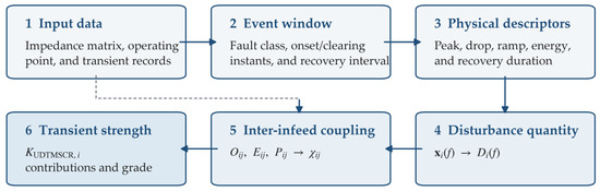
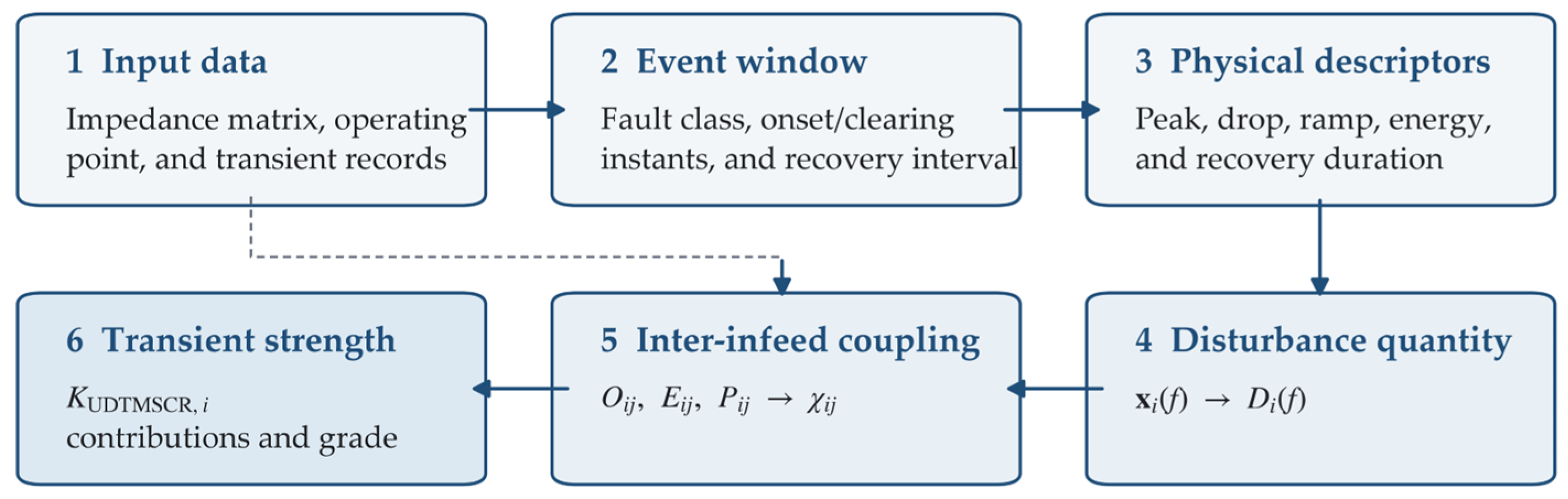
Figure 1 gives the numerical sequence. The impedance matrix and transient records are first assembled, after which the event window is selected according to the fault class. The six descriptors are calculated and combined into $D_i(f)$. The overlap and electrical-proximity terms determine ${\chi }_{ij}(f)$, and the resulting disturbance terms are inserted into the impedance-weighted denominator to obtain $K_{UDTMSCR,i}(f)$ and its local and mutual contributions.

Figure 1. Computational sequence for fault-disturbance extraction and UDTMSCR evaluation.

The same procedure can be applied to planning simulations and post-event records. Planning studies obtain the required trajectories from electromechanical or electromagnetic-transient models, whereas event analysis uses synchronized measurements. For near-real-time assessment, the parameters and thresholds must be fixed before the event under study and updated only when the network model or operating range changes materially.

4.2. Fault-Template Switching

The weights in (10) should not be fixed blindly for all events. Table 2 gives the recommended template interpretation. The values are not universal constants; they define the physical emphasis of each fault class and can be calibrated by historical or simulated samples. In the numerical study of Section 5, one common weight set is applied to all fault classes so that the differences among classes originate from the trajectories alone; the class-specific emphasis listed in Table 2 then appears in the descriptor values themselves, and class-specific weights remain an optional calibration.

Table 2. Fault-template interpretation for unified disturbance extraction.

Fault Class	Dominant Terms	Suggested Window	Physical Emphasis
DC bipolar blocking	${\widehat{Q}}_i^{pk}$, ${\widehat{E}}_i^Q$, ${\widehat{T}}_i^{rec}$	Blocking trigger to voltage recovery	Reactive-consumption disappearance, filter surplus, and overvoltage duration.
Commutation failure	${\widehat{R}}_i^Q$, ${\widehat{Q}}_i^{pk}$, ${\widehat{T}}_i^{rec}$	Failure onset to commutation recovery	Rapid control-angle and reactive-power variation.
AC-fault clearing	${\widehat{P}}_i^{drop}$, ${\widehat{E}}_i^Q$, ${\widehat{T}}_i^{rec}$	Fault clearing and post-fault recovery	Power-transfer drop, reactive recovery, and voltage-recovery delay.
Coupled multi-infeed disturbance	${\widehat{Q}}_i^{pk}$, ${\widehat{R}}_i^Q$, ${\widehat{C}}_i^f$	First affected infeed to last recovery	Synchronized disturbance and mutual-impedance transfer.

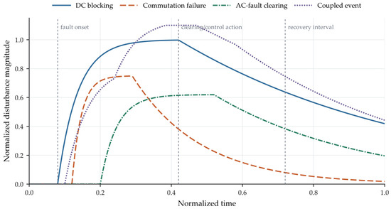
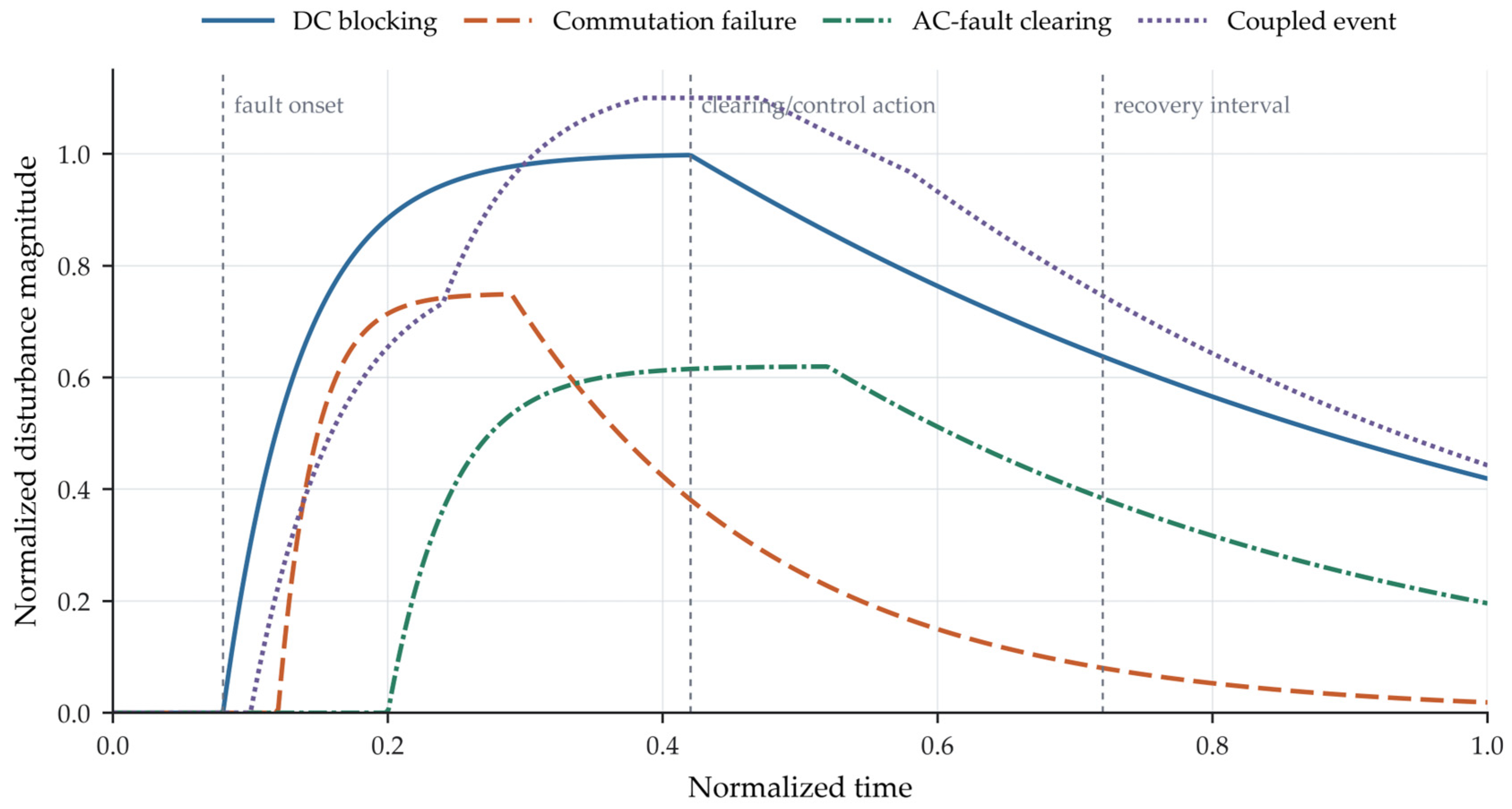
Figure 2 illustrates the qualitative disturbance signatures. A blocking event is dominated by a high-amplitude disturbance with a visible recovery tail. A commutation-failure event may be shorter but sharper. An AC-fault-clearing event has a stronger recovery component, and a coupled multi-infeed event combines local and neighboring disturbances.

Figure 2. Representative normalized disturbance signatures for different fault templates.

4.3. Numerical Implementation

The calculation is performed in six steps. First, obtain $Z_{eq}$ and the pre-fault operating quantities of all HVDC infeeds. Second, identify the fault class and select the evaluation interval $\left[t_0,t_1\right]$. Third, extract $Q_i(t)$, $P_i(t)$, and any available control-angle or protection-timestamp records. Fourth, calculate the normalized terms in (4)–(8) and apply (9)–(10). Fifth, calculate $O_{ij}$, $E_{ij}$, and, when available, $P_{ij}$; form ${\chi }_{ij}(f)$; evaluate (13); and separate the local and mutual terms using (14). Sixth, rank the cases by transient strength and, when required, apply (15) and (16) with the selected retrospective or prospective interpretation.

This procedure intentionally separates model structure from calibration. The formula structure is fixed, whereas ${\lambda }_f$, ${\eta }_i$, the feature weights, ${\chi }_{ij}(f)$, and the grading thresholds can be tuned for a specific grid. Such separation is important because receiving grids differ in compensation equipment, control settings, and protection logic.

The disturbance-window boundaries have a direct influence on the calculated descriptors. An early start includes pre-fault fluctuations, whereas an unnecessarily late endpoint can include unrelated dispatch or compensation changes. The following rule is used for every compared case. The start $t_0$ is the earlier of the first fault or protection timestamp and the first sample at which $\left|Q_i(t)-Q_i(t_0^{-})\right|$ exceeds the tolerance band ${\epsilon }_Q{S}_{base,i}$, reduced by a backward margin of 20 ms so that the steepest part of the ramp is never truncated; the pre-fault reference $Q_i(t_0^{-})$ is the mean value over the 100 ms preceding $t_0$. The end $t_1$ is the first instant after the peak at which the deviation has remained inside the tolerance band for 50 ms, bounded by the maximum horizon $t_0+T_{max}$ ($T_{max}$ = 1.8 s here); if the band is not reached, $t_1=t_0+T_{max}$ and the recovery descriptor is capped as stated after (8). Because the energy term uses the fixed base $T_f$, extending the window beyond $t_1$ leaves the descriptors unchanged, and Section 5.6 quantifies the effect of shifting $t_0$ or truncating $t_1$.

The calculation can also be applied when measurement channels are incomplete. If reactive power is directly available, (4), (6), and (7) are evaluated from the measured reactive-power series. Otherwise, (11) and (12) provide an approximate reconstruction from active power and converter-angle records. If neither converter-angle trajectories nor reactive-power telemetry are available, the disturbance vector is underdetermined and the method should be restricted to offline planning studies with simulated trajectories.

Reported results should include the proposed index $K_{UDTMSCR,i}(f)$, the conventional $K_{MSCR,i}$ as a static baseline, the self contribution $C_{ii}$, and the largest mutual contribution $C_{ij}$. A scalar index alone does not distinguish a weak local condition from the influence of a disturbed neighboring station; the contribution terms provide this distinction directly. The complete reporting format, the required and optional measurement channels, the fallback approximations, and the recommended sampling rate are summarized.

5. Case Studies and Experimental Analysis

5.1. Two-Infeed Mechanism Model

A two-infeed equivalent model is used to validate the proposed index. The model contains two LCC-HVDC infeeds connected to a receiving AC system through equivalent impedances $Z_1$, $Z_2$, and $Z_{12}$. The first converter bus is the evaluated fault-side bus, while the second converter bus represents a neighboring infeed that may remain quiet or experience a synchronized disturbance. The equivalent self- and mutual-impedance terms are:

$$|Z_{eq,11}|={\displaystyle \frac{\left|Z_1{Z}_2|+|Z_1{Z}_{12}\right|}{\left|Z_1|+|Z_2|+|Z_{12}\right|}}$$

(17)

$$|Z_{eq,12}|={\displaystyle \frac{\left|Z_1{Z}_2\right|}{\left|Z_1|+|Z_2|+|Z_{12}\right|}}$$

(18)

The dynamic voltage response is represented by a first-order recovery link:

$${\tau }_v{\displaystyle \frac{d\Delta U_i(t)}{dt}}+\Delta U_i(t)=k_v\left(|Z_{eq,ii}|u_i(t)+{\sum }_{j=1,j\ne i}^n|Z_{eq,ij}|u_j(t)\right)$$

(19)

where $\Delta U_i(t)$ is the voltage deviation of converter bus $i$, ${\tau }_v$ is the voltage-recovery time constant, $k_v$ is the voltage-disturbance gain, and the normalized disturbance input is $u_i(t)$.

The mechanism model is deliberately compact and is not intended to reproduce all electromagnetic details of an LCC-HVDC converter.

It is used to test whether the proposed index changes consistently with transient voltage severity when the local impedance, mutual impedance, fault class, and neighboring disturbance are varied.

For the two-infeed case, the conventional denominator is obtained by inserting the equivalent impedances in (17) and (18) into (2). The proposed denominator uses the same impedance terms but replaces the rated-power quantities by $D_1$ and $D_2$. Thus, any difference between the two indices is caused by the disturbance representation rather than by a change in the network equivalent. This controlled comparison is useful because it isolates the benefit of the disturbance-driven denominator.

The first-order recovery relation in (19) is a reduced-order approximation of the dominant voltage response. It does not represent valve commutation, firing-angle limiters, or detailed AC-protection logic. Its purpose is limited to testing whether an increase in impedance-weighted disturbance produces the expected increase in temporary voltage deviation and whether the proposed index preserves the ordering of the studied cases.

5.2. Scenario Configuration

Eight scenarios are constructed from the available program and result data. The time step is 0.001 s, the simulation horizon is 2.0 s, the disturbance starts at 0.20 s, and the nominal disturbance plateau ends at 0.55 s. The voltage gain is $k_v=0.72$, and the recovery time constant is ${\tau }_v=0.055$ s. Blocking, commutation-failure, AC-fault-clearing, and coupled-disturbance profiles use different rise and decay parameters.

The disturbance input used in the mechanism simulation is expressed as a normalized profile multiplied by the normalized reactive-power peak deviation of (4), so that the voltage model is driven by the reactive-power trajectory and not by the composite index:

$$u_i(t)={\widehat{Q}}_i^{pk}{s}_i(t;f)$$

(20)

where $s_i(t;f)$ is a unitless temporal shape associated with the fault class. In the implemented cases, the shape is represented by a rise-hold-recovery profile:

$$s_i(t;f)=\left\{\begin{array}{cc}0,& t<t_0,\\ 1-\mathrm{e}\mathrm{x}\mathrm{p}[-(t-t_0)/{\tau }_{r,f}],& t_0\le t<t_h,\\ \mathrm{e}\mathrm{x}\mathrm{p}[-(t-t_h)/{\tau }_{d,f}],& t\ge t_h,\end{array}\right.$$

(21)

where ${\tau }_{r,f}$ is the rise time constant, ${\tau }_{d,f}$ is the decay time constant, and $t_h$ is the end of the nominal disturbance plateau. Blocking cases use a large $D_1$ and a slower decay tail, commutation-failure cases use a sharper rise and lower energy, and AC-fault-clearing cases emphasize recovery. The time constants are (${\tau }_{r,f}$, ${\tau }_{d,f}$) = (0.035, 0.180) s for blocking, (0.020, 0.090) s for commutation failure, and (0.030, 0.140) s for AC-fault clearing, with $t_h$ = 0.55 s in all classes; the neighboring infeed uses the same shape as the fault-side infeed in each case. The coupled blocking case assigns a material $D_2$ to the neighboring infeed, so that the mutual term in (13) becomes active.

The voltage peak used for comparison is calculated from the simulated voltage-deviation trajectory:

$$V_i^{pk}=1+{max}_{t\in [t_0,t_1]}\Delta U_i(t)$$

(22)

This definition is consistent with the per-unit curves in Figure 3. The index comparison is then made using the inverse strength values because a smaller strength index corresponds to a weaker and higher-risk condition:

$${\rho }_P=corr\left({\displaystyle \frac{1}{K_i}},V_i^{pk}\right),{\rho }_S=rankcorr\left({\displaystyle \frac{1}{K_i}},V_i^{pk}\right)$$

(23)

where ${\rho }_P$ is the Pearson correlation and ${\rho }_S$ is the Spearman rank correlation. The Pearson coefficient checks linear consistency with voltage peak, while the Spearman coefficient checks whether the index preserves the ordering of scenario severity.

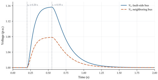
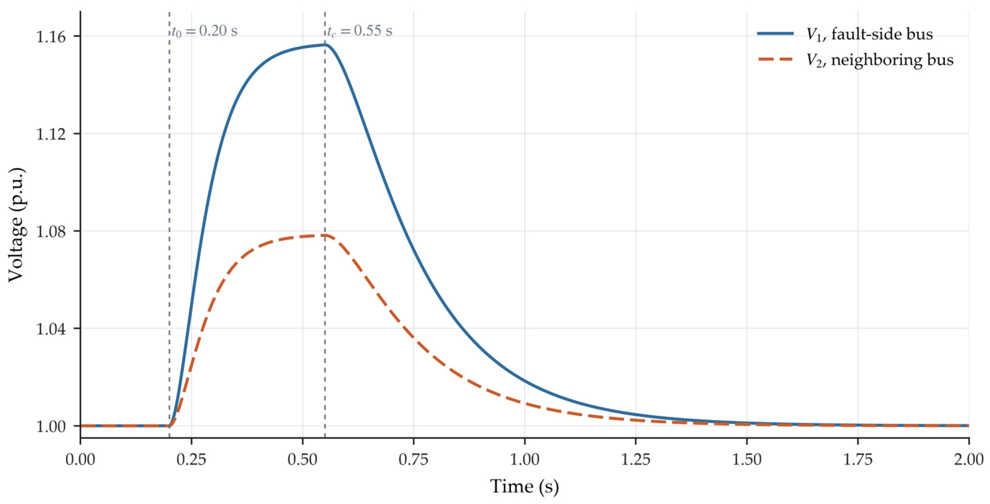
Figure 3. Simulated voltage response of the base two-infeed blocking scenario.

The base blocking voltage response is shown in Figure 3. The fault-side converter bus reaches a higher peak than the neighboring bus because the first infeed carries the main disturbance, while the second infeed is affected through mutual coupling only.

Table 3 lists the scenario parameters and calculated results. Each case label identifies the corresponding fault class and parameter change, and the UDTMSCR1 column reports the proposed index value; the descriptor values from which $D_1$ and $D_2$ are obtained are given in Table 4.

Table 3. Two-infeed mechanism cases and calculated transient-strength results.

Case	Fault Type	${\mathit{Z}}_1$	${\mathit{Z}}_2$	${\mathit{Z}}_{12}$	${\mathit{D}}_1$	${\mathit{D}}_2$	MSCR1	UDTMSCR1	V1 Peak
S1 block base	blocking	0.300	0.400	0.400	0.850	0.020	3.056	5.326	1.156
S1 block high $Z_1$	blocking	0.450	0.400	0.400	0.850	0.020	2.315	4.035	1.206
S1 block high $Z_2$	blocking	0.300	0.550	0.400	0.850	0.020	2.778	5.088	1.163
S1 block high $Z_{12}$	blocking	0.300	0.400	0.650	0.850	0.020	3.103	4.994	1.167
S1 commutation failure base	commutation failure	0.300	0.400	0.400	0.593	0.020	3.056	7.602	1.097
S1 commutation failure high $Z_1$	commutation failure	0.450	0.400	0.400	0.593	0.020	2.315	5.759	1.128
S1 AC clearing base	AC-fault clearing	0.300	0.400	0.400	0.676	0.280	3.056	5.617	1.124
S1–S2 coupled block	blocking	0.300	0.400	0.300	0.850	0.641	3.030	3.913	1.211

Table 4. Normalized descriptors and unified disturbance quantities of the eight representative cases (weights $w$ = (0.45, 0.20, 0.15, 0.10, 0.10, 0); ${\tau }_f$ = 0.02 s; $T_f$ = $T_{ref}$ = 0.45 s; descriptor cap 1.5; floor 0.02).

Trajectory (Table 3 Rows)	${\widehat{\mathit{Q}}}_{\mathit{i}}^{\mathit{p}\mathit{k}}$	${\widehat{\mathit{P}}}_{\mathit{i}}^{\mathit{d}\mathit{r}\mathit{o}\mathit{p}}$	${\widehat{\mathit{R}}}_{\mathit{i}}^{\mathit{Q}}$	${\widehat{\mathit{E}}}_{\mathit{i}}^{\mathit{Q}}$	${\widehat{\mathit{T}}}_{\mathit{i}}^{\mathit{r}\mathit{e}\mathit{c}}$	${\widehat{\mathit{C}}}_{\mathit{i}}^{\mathit{f}}$	${\mathit{D}}_{\mathit{i}}$
Blocking, fault-side infeed (rows 1–4 and 8)	1.000	0.280	0.563	1.100	1.500	0	0.850
Commutation failure, fault-side infeed (rows 5–6)	0.620	0.210	0.605	0.579	1.233	0	0.593
AC-fault clearing, fault-side infeed (row 7)	0.700	0.360	0.459	0.716	1.487	0	0.676
AC-fault clearing, neighboring infeed (row 7)	0.180	0.070	0.118	0.184	1.487	0	0.280
Coupled blocking, neighboring infeed (row 8)	0.700	0.200	0.394	0.770	1.500	0	0.641
Undisturbed neighboring infeed (rows 1–6)	0	0	0	0	0	0	0.020

The eight scenarios are designed to separate different physical effects. The base blocking case is the reference condition. The high-$Z_1$ case weakens the local path while keeping the disturbance unchanged. The high-$Z_2$ case changes the neighboring self-impedance but keeps the neighboring disturbance small. The high-$Z_{12}$ case changes the mutual path, which tests whether the index responds to stronger coupling. The two commutation-failure cases reduce the disturbance magnitude but keep the sharp fault character. The AC-clearing case uses a moderate local disturbance and a non-negligible neighboring recovery component. The coupled blocking case activates the neighboring infeed as a major disturbance source.

For the eight representative cases in Table 3, ${\chi }_{12}=1$ is retained as a conservative upper bound. This controlled setting isolates the effect of replacing rated power by the trajectory-based quantity $D_j$. In the parametric study, ${\chi }_{12}$ is instead calculated from the overlap and impedance terms.

Table 4 documents how $D_1$ and $D_2$ in Table 3 are obtained from (4)–(10), so that every case can be reconstructed. The reactive-power trajectory of each infeed is $u_i(t)$ in (20), its peak deviation is ${\widehat{Q}}_i^{pk}$, and the active-power drop ${\widehat{P}}_i^{drop}$ is prescribed for each case because the mechanism model does not simulate the active-power trajectory (0.28 for blocking, 0.21 for commutation failure, and 0.36 for AC-fault clearing at the fault-side infeed; 0.07 and 0.20 at the neighboring infeed in the AC-clearing and coupled cases). The ramp descriptor uses ${\tau }_f$ = 0.02 s, the energy descriptor uses $T_f$ = 0.45 s, the recovery descriptor uses $T_{ref}$ = 0.45 s with a tolerance band equal to 10% of the peak deviation, and each of the three shape-dependent descriptors is capped at 1.5. The weights are $w$ = (0.45, 0.20, 0.15, 0.10, 0.10, 0), ${\lambda }_f={\eta }_i=1$, $S_{base,i}$ = 1 p.u., and $D_i$ is floored at 0.02 for an undisturbed infeed. For the base blocking case, $D_1$ = 0.45 × 1.000 + 0.20 × 0.280 + 0.15 × 0.563 + 0.10 × 1.100 + 0.10 × 1.500 = 0.850. The class-specific emphasis of Table 2 is visible in the descriptors: the commutation-failure trajectory has the largest ramp descriptor, the blocking trajectory the largest energy and recovery descriptors, and the AC-clearing trajectory the largest active-power drop.

5.3. Correlation with Transient Voltage Peaks

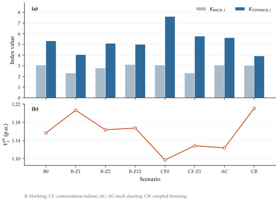
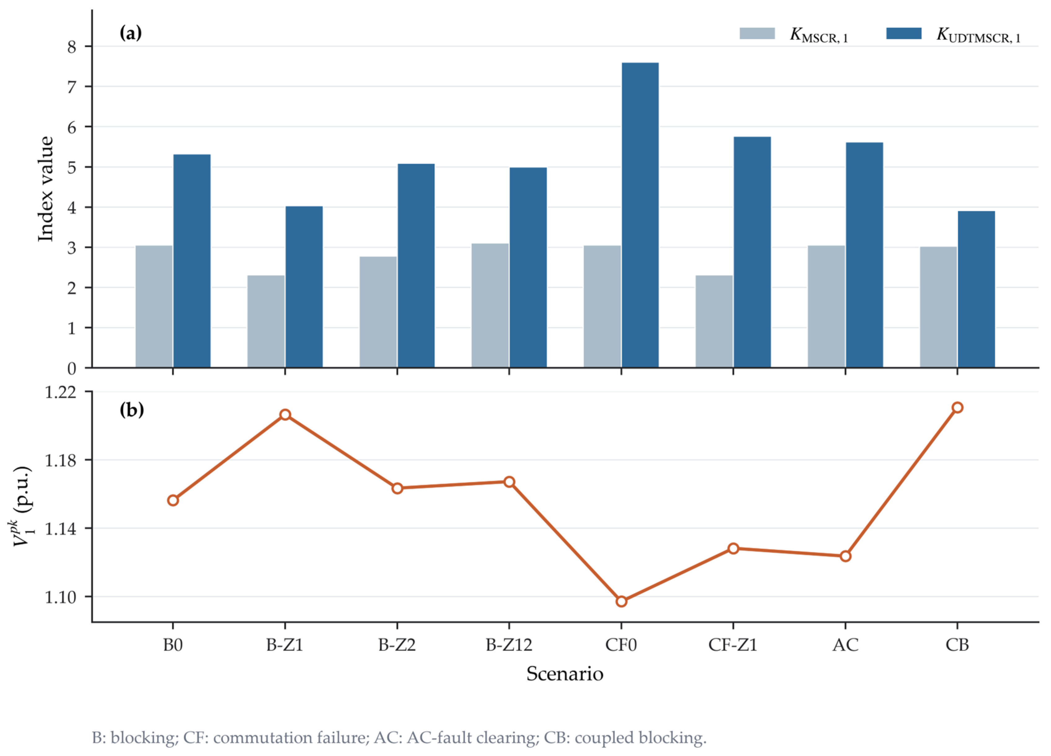
Figure 4 presents the two strength indices and the fault-side voltage peak on separate panels. Increasing the local impedance $Z_1$ lowers both indices and raises the voltage peak from 1.156 to 1.206 p.u. Increasing $Z_{12}$ produces a small increase in conventional MSCR for the equivalent used here even though the voltage peak rises. UDTMSCR instead decreases from 5.326 to 4.994, in agreement with the observed risk direction.

Figure 4. Results for the eight representative cases: (a) conventional MSCR and UDTMSCR; (b) fault-side voltage peak. B, blocking; CF, commutation failure; AC, AC-fault clearing; CB, coupled blocking.

Across the eight cases, the Pearson correlation between $1/K_{UDTMSCR,1}$ and $V_1^{pk}$ is 0.979 and the Spearman rank correlation is 0.976. The corresponding values for $1/K_{MSCR,1}$ are 0.193 and 0.246. For the blocking subset, the Pearson and Spearman correlations for inverse UDTMSCR are both 1.000, compared with 0.480 and 0.300 for inverse MSCR. Thus, in the present two-infeed cases, the disturbance-based denominator follows the voltage-severity ordering more closely than the rated-power denominator.

The difference between the two correlation results is significant for interpretation. Conventional MSCR changes only when the impedance parameters or rated-power assumptions change. It is therefore insensitive to whether a neighboring infeed is actually disturbed during the fault process. This insensitivity is not a deficiency of MSCR within its intended static scope; it is precisely the information that a static index cannot carry, and the transient reference indices introduced at the end of this section complement the comparison. By contrast, UDTMSCR changes when either the impedance path or the disturbance quantity changes. The coupled blocking case is the clearest example: the conventional index remains close to the base value, but the proposed index decreases because the neighboring disturbance enters the denominator through $D_2$ and ${\chi }_{12}(f)$.

Both Pearson and Spearman coefficients are reported because a planning index need not vary linearly with voltage peak to be useful; it should, however, preserve the ordering of severe cases. In the present data, inverse UDTMSCR nearly preserves this ordering, whereas inverse MSCR does not. This property is useful when a large set of contingencies must be reduced before detailed electromagnetic-transient calculation.

Because MSCR was not developed for transient response, two additional references are included. The first is a peak-only transient index of the same impedance-weighted family, obtained by replacing the rated powers in (2) by the normalized reactive-power peak deviations of (4):

$$K_{Q,i}(f)={\displaystyle \frac{1}{\left|Z_{eq,ii}\right|{\widehat{Q}}_i^{pk}+{\sum }_{j=1,j\ne i}^n\left|Z_{eq,ij}\right|{\widehat{Q}}_j^{pk}{\chi }_{ij}(f)}}$$

(24)

This index corresponds to the reactive-surplus estimate of temporary overvoltage that is commonly used in blocking and commutation-failure studies [19,20], and it isolates the contribution of the ramp, energy, and recovery descriptors in $D_i(f)$. The second reference is a transient voltage severity index of the type used in short-term voltage-stability assessment [25], evaluated from the simulated fault-side voltage as

$${\mathrm{T}\mathrm{V}\mathrm{S}\mathrm{I}}_i={\displaystyle \frac{1}{t_1-t_0}}{\int }_{t_0}^{t_1}\left|\Delta U_i(t)\right|H\left(\left|\Delta U_i(t)\right|−\mu \right)dt$$

(25)

where $H(·)$ is the unit step function and $\mu$ = 0.05 p.u. is the deviation threshold. TVSI is an outcome measure that weights both the magnitude and the duration of the voltage excursion; it is used as a second severity benchmark, not as a strength index. In the impedance form used here, the multi-infeed interactive effective short-circuit ratio of [23] reduces to (2), because the interaction factor equals $\left|Z_{eq,ji}\right|/\left|Z_{eq,ii}\right|$; it is therefore represented by the MSCR row. Commutation-failure immunity indices [24] require valve-level fault sweeps that the reduced-order model cannot provide and are reserved for the electromagnetic-transient study described in Section 5.5.

Table 5 summarizes the correlations. Both transient indices follow the voltage peak and the TVSI closely, whereas the static index does not. Because ${\chi }_{12}$ = 1 in the eight cases, the difference between the static and the transient indices there originates entirely from the trajectory-based disturbance description and not from the coupling coefficient. Between the two transient indices the differences are within 0.03: the peak-only index gives a slightly higher Pearson correlation with the voltage peak, whereas UDTMSCR gives the higher rank correlation with the TVSI in the eight cases. This outcome is expected from the mechanism model, in which the voltage is a linear first-order response to the reactive-power trajectory, so that the voltage peak is governed almost entirely by the disturbance amplitude and the ramp, energy, and recovery descriptors can influence only duration-related severity. The reduced-order study therefore discriminates between static and transient disturbance descriptions and quantifies the effect of the participation coefficient in Section 5.5, but it cannot establish the added value of the ramp, energy, and recovery terms over a peak-only transient descriptor; that question is reserved for the electromagnetic-transient cases listed in Section 5.5, in which commutation and recovery dynamics are represented explicitly.

Table 5. Pearson (${\rho }_P$) and Spearman (${\rho }_S$) correlations between the inverse indices and the two severity benchmarks for the eight representative cases (${\chi }_{12}$ = 1) and the 48 parametric cases (${\chi }_{12}$ from (15)).

Inverse Index	Case Set	Voltage Peak, ${\mathit{\rho }}_{\mathit{P}}$	Voltage Peak, ${\mathit{\rho }}_{\mathit{S}}$	TVSI, ${\mathit{\rho }}_{\mathit{P}}$	TVSI, ${\mathit{\rho }}_{\mathit{S}}$
Conventional MSCR, (2)	eight cases	0.193	0.246	0.146	0.135
Peak-only transient index, (24)	eight cases	1.000	1.000	0.998	0.976
UDTMSCR, (13)	eight cases	0.979	0.976	0.970	1.000
Conventional MSCR, (2)	48 cases	−0.294	−0.310	−0.253	−0.320
Peak-only transient index, (24)	48 cases	0.979	0.975	0.966	0.959
UDTMSCR, (13)	48 cases	0.973	0.983	0.959	0.951

5.4. Interpretation of Representative Scenarios

The base blocking case has $D_1=0.850$ and $D_2=0.020$, so the first infeed dominates the denominator. When $Z_1$ increases from 0.300 to 0.450, $UDTMSC{R}_1$ drops by 1.291 and the voltage peak rises by 0.050 p.u. This is the expected result for a locally weakened receiving grid.

When $Z_2$ increases, the voltage peak rises only moderately, from 1.156 p.u. to 1.163 p.u., because the neighboring infeed carries only a small disturbance. The proposed index decreases by 0.239, reflecting a limited but nonzero influence. This behavior is useful because it avoids treating every neighboring infeed at full rated disturbance level.

The high-$Z_{12}$ case is more revealing. The conventional $MSC{R}_1$ changes from 3.056 to 3.103, which would suggest a slightly stronger condition in the studied equivalent expression. However, the voltage peak rises from 1.156 p.u. to 1.167 p.u. The proposed $UDTMSC{R}_1$ moves in the physically consistent direction by decreasing from 5.326 to 4.994. This result illustrates why transient disturbance and coupling must be evaluated together.

The coupled blocking case has the highest voltage peak, 1.211 p.u., even though $MSC{R}_1$ is close to the base value. The reason is that $D_2$ increases from 0.020 to 0.641, so the neighboring infeed becomes an active disturbance source. Equation (13) captures this through the mutual-impedance term, whereas the conventional rated-power denominator does not distinguish whether the neighbor is actually disturbed.

The commutation-failure cases provide a complementary observation. Their local disturbance value is lower than that of the blocking case, and their voltage peaks are also lower in the studied mechanism model. However, the commutation-failure template gives attention to the ramp component, so the disturbance quantity is not reduced simply in proportion to peak amplitude. This is consistent with the physical fact that commutation failure may be short but severe in its rate of change.

The AC-fault-clearing case shows the role of recovery-related terms. Its $D_1$ value lies between the blocking and commutation-failure values, while $D_2$ is no longer negligible. The resulting UDTMSCR1 value, 5.617, lies above the base blocking value of 5.326 and well above the coupled blocking value of 3.913, which matches the ordering of the corresponding voltage peaks of 1.124, 1.156, and 1.211 p.u. This ranking is consistent with a fault-clearing process that has a visible recovery component but does not activate the neighboring infeed as strongly as the coupled blocking scenario.

5.5. Parametric Sensitivity to Event Timing and Electrical Distance

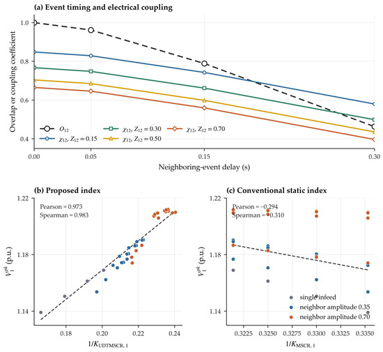
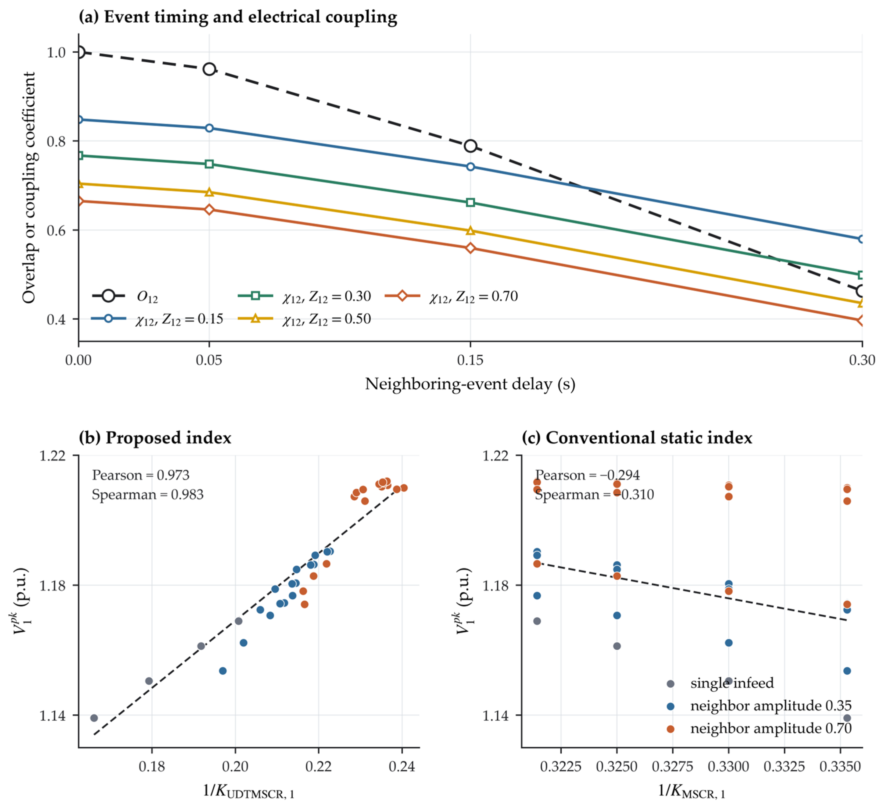
The sensitivity of the coupling coefficient is examined with 48 additional blocking cases derived from the same two-infeed equations. The study combines four mutual-path values $Z_{12}\in \left\{\mathrm{0.15,\; 0.30,\; 0.50,\; 0.70}\right\}$, four neighboring-event delays $\Delta t\in \left\{\mathrm{0,\; 0.05,\; 0.15,\; 0.30}\right\}$ s, and three neighboring-disturbance amplitudes $q_2^{pk}\in \left\{\mathrm{0,\; 0.35,\; 0.70}\right\}$. The local and neighboring self paths, local disturbance, integration step, and recovery parameters are held at their base values. Because the model does not provide protection timestamps, $w_O=w_E=0.5$ and $w_P=0$ are used throughout this study.

Across these 48 cases (Figure 5.), ${\chi }_{12}$ ranges from 0.165 to 0.848, the fault-side voltage peak ranges from 1.139 to 1.212 p.u., and UDTMSCR ranges from 4.159 to 6.021. The Pearson and Spearman correlations between $1/K_{UDTMSCR,1}$ and $V_1^{pk}$ are 0.973 and 0.983, respectively. For $1/K_{MSCR,1}$, the corresponding values are −0.294 and −0.310 because the static baseline cannot respond to neighboring-event timing or amplitude and, in this equivalent, its mutual-path trend is opposite to the voltage-risk trend.

Figure 5. Parametric sensitivity of the inter-infeed coupling representation: (a) disturbance overlap and coupling coefficient for four mutual-path values; (b) inverse UDTMSCR versus voltage peak; and (c) inverse conventional MSCR versus voltage peak.

For the strongest neighboring disturbance, increasing the delay from 0 to 0.30 s reduces the mean overlap from 1.000 to 0.463 and the mean coupling coefficient from 0.746 to 0.478 across the four electrical-distance settings. The mean fault-side voltage peak consequently falls from 1.2110 to 1.1804 p.u., while the mean inverse UDTMSCR falls from 0.2372 to 0.2184. This monotonic response demonstrates that the coefficient distinguishes synchronized multi-infeed stress from a temporally separated neighboring event.

The parametric results broaden the range of event timing and electrical distance considered here, but they do not constitute a valve-level electromagnetic-transient validation. The available model contains impedance gains and first-order recovery links rather than converter bridges, current and extinction-angle controls, VDCOL, firing-pulse generation, transformer saturation, AC filters, and protection logic. A subsequent detailed study should retain the post-processing equations while obtaining trajectories from PSCAD/EMTDC, RTDS, or an equivalent EMT model. The required cases include single-station blocking, single and successive commutation failures, AC-fault clearing at several electrical distances, filter or capacitor switching, and delayed multi-infeed events.

5.6. Sensitivity to Weights, Thresholds, Event Window, and Record Imperfections

The disturbance weights in (10) were not calibrated on independent events; the numerical study uses the single engineering setting $w$ = (0.45, 0.20, 0.15, 0.10, 0.10, 0). Table 6 reports how the correlation between inverse UDTMSCR and the fault-side voltage peak changes when this setting is varied. Four alternative settings that emphasize equal weighting, amplitude, ramp, or energy and recovery, ten one-at-a-time perturbations of ±50% of each weight with renormalization, and 500 weight sets drawn uniformly from the simplex were evaluated. The one-at-a-time perturbations keep the Pearson correlation between 0.956 and 0.991 for the eight cases and between 0.966 and 0.979 for the 48 cases, and the Spearman correlation between 0.929 and 1.000 and between 0.982 and 0.984, respectively. Over the 500 random sets the median Spearman correlation is 0.917 for the eight cases and 0.978 for the 48 cases; the correlation deteriorates only when the recovery-duration weight exceeds about 0.4, because the capped duration term then dominates $D_i(f)$ and the cases become indistinguishable. When the reactive-peak weight is at least 0.3, the Spearman correlation remains above 0.74 for the eight cases and above 0.91 for the 48 cases in all 142 such sets. The amplitude-dominant setting adopted here is therefore not a tuned choice but a physically motivated region within which the ordering is stable.

Table 6. Sensitivity of the Pearson (${\rho }_P$) and Spearman (${\rho }_S$) correlations between inverse UDTMSCR and the fault-side voltage peak to the disturbance weights, coupling weights, event window, and record imperfections (– indicates a setting that is not applicable to the case set).

Setting	Eight Cases, ${\mathit{\rho }}_{\mathit{P}}$	Eight Cases, ${\mathit{\rho }}_{\mathit{S}}$	48 Cases, ${\mathit{\rho }}_{\mathit{P}}$	48 Cases, ${\mathit{\rho }}_{\mathit{S}}$
Disturbance weights, base (0.45, 0.20, 0.15, 0.10, 0.10)	0.979	0.976	0.973	0.983
Disturbance weights, equal (0.20 each)	0.932	0.857	0.953	0.977
Disturbance weights, amplitude only (0.70, 0.30, 0, 0, 0)	0.998	0.976	0.979	0.974
Disturbance weights, ramp-weighted (0.30, 0.15, 0.35, 0.10, 0.10)	0.959	0.976	0.972	0.984
Disturbance weights, energy/recovery-weighted (0.30, 0.10, 0.10, 0.25, 0.25)	0.943	0.929	0.949	0.973
Disturbance weights, ±50% one-at-a-time (range over ten sets)	0.956–0.991	0.929–1.000	0.966–0.979	0.982–0.984
Disturbance weights, 500 random sets (5th percentile/median)	0.692/0.937	0.619/0.917	0.881/0.962	0.890/0.978
Coupling weights, overlap only ($w_O$ = 1)	–	–	0.985	0.994
Coupling weights, $w_O$ = 0.75, $w_E$ = 0.25	–	–	0.984	0.990
Coupling weights, $w_O$ = 0.25, $w_E$ = 0.75	–	–	0.946	0.958
Coupling weights, proximity only ($w_E$ = 1)	–	–	0.889	0.898
Coupling coefficient fixed, ${\chi }_{12}$ = 1	–	–	0.912	0.933
Event window, $t_0$ shifted by −20 ms	0.979	0.976	–	–
Event window, $t_0$ shifted by +20 ms	0.983	0.976	–	–
Event window, $t_1$ = 1.0 s	0.978	0.976	–	–
Event window, $t_1$ = 0.7 s	0.978	1.000	–	–
Record imperfections, noise at 20 dB signal-to-noise ratio	–	–	0.977	0.981
Record imperfections, noise at 10 dB signal-to-noise ratio	–	–	0.955	0.954
Record imperfections, misalignment of ±20 ms	–	–	0.971–0.975	0.980–0.984
Record imperfections, 30% missing samples	–	–	0.973	0.983

The coupling weights in (15) were varied from an overlap-only estimator to a proximity-only estimator, and the fixed value ${\chi }_{12}$ = 1 was also examined. For the voltage peak the correlation increases with the overlap weight, from a Pearson value of 0.889 with $w_E$ = 1 to 0.985 with $w_O$ = 1, and ${\chi }_{12}$ = 1 gives 0.912; for the TVSI the ordering is reversed and ${\chi }_{12}$ = 1 gives the highest values, 0.992 and 0.997. The two results are consistent: a delayed neighboring disturbance contributes little to the peak but contributes fully to the time integral of the voltage excursion. The participation coefficient should therefore be chosen according to the severity measure of interest, with overlap-weighted estimation for peak-type assessment and values close to unity for energy- or duration-type assessment. The electrical-proximity term is not the source of the improvement over MSCR; it only moderates the participation of an electrically remote neighbor, and the conclusions of Section 5.3, Section 5.4 and Section 5.5 are unchanged when it is removed.

The influence of the grading thresholds in (16) was examined by assigning the 48 cases to three grades with the 50th and 80th percentiles of inverse UDTMSCR and comparing the result with the grades obtained from the voltage peak with the same percentiles. The two gradings agree for 42 of the 48 cases (87.5%), whereas the agreement is 35.4% for inverse MSCR. With the 33rd and 67th percentiles the agreement is 97.9%, and with the 50th and 90th percentiles it is 83.3%. Over 200 random weight sets the agreement remains between 70.8% and 87.5%, with a median of 87.5%.

The event-window rule of Section 4.3 was tested on the eight cases. Starting the window 20 ms before the fault instant leaves every descriptor unchanged, whereas starting it 20 ms after the fault instant truncates the steepest part of the ramp and reduces $D_1$ of the blocking cases from 0.850 to 0.813. Ending the window at 1.5 s, 1.0 s, 0.8 s, or 0.7 s instead of 2.0 s changes $D_1$ of the blocking cases by 0.0002, 0.003, 0.027, and 0.057, respectively, because the fixed base $T_f$ in (7) makes the energy term insensitive to the window length once the disturbance has returned to its tolerance band. The correlations remain above 0.977 (Pearson) and 0.976 (Spearman) in all window settings. The window must therefore begin at or before the first deviation, for which the protection timestamp with a backward margin is adequate, and must extend beyond the return to the tolerance band; further extension has no material effect.

The robustness of the coupling coefficient to imperfect records was assessed on the 48 cases by corrupting the normalized envelopes used in (15). Additive white noise with a signal-to-noise ratio of 20 dB, after gating the envelope where a 20-ms moving average stays below 10% of its peak, changes ${\chi }_{12}$ by 0.031 on average and by 0.092 at most, and the correlations become 0.977 and 0.981; at 10 dB the mean change is 0.144 and the correlations decrease to 0.955 and 0.954. A timing misalignment of ±10 ms or ±20 ms between the two records changes ${\chi }_{12}$ by at most 0.011 and 0.023, respectively. Randomly missing samples of 10% and 30%, reconstructed by holding the last value, change ${\chi }_{12}$ by less than 0.001. The overlap term is therefore tolerant to the timing errors and gaps expected from synchronized fault recorders, and moderate noise is handled by the envelope gating; when a neighboring record is unavailable, ${\chi }_{12}$ should be reported with the proximity term only and flagged as a lower-confidence value.

5.7. Engineering Implications and Limitations

The impedance-matrix form of UDTMSCR preserves the familiar self- and mutual-coupling interpretation of MSCR, while the trajectory-derived terms distinguish different fault classes within one expression. Separation of the denominator into local and mutual contributions further indicates whether a weak condition is associated with local grid impedance, a disturbed neighboring infeed, reactive-power deviation, a rapid power change, or slow recovery.

The present validation contains eight representative cases and a 48-case parametric study, all obtained from a reduced-order two-infeed model. The fault-dependent weights and the overlap/electrical-proximity weights have a direct physical interpretation, but their numerical values must be determined for the receiving grid under study. Because valve commutation, detailed converter controls, AC protection, and compensation switching are not modeled, the reported values establish trends and case ordering rather than universal operating thresholds. Two further limitations should be stated explicitly. First, no detailed electromagnetic-transient validation has been performed; the mechanism model represents the voltage response by a first-order link and cannot reproduce commutation dynamics, current-order limiter action, filter switching, or protection sequences, so the ranking evidence is limited to trends and case ordering, and the comparison in Table 5 cannot separate the six-descriptor quantity from a peak-only transient descriptor. Second, no field disturbance record could be included, because synchronized fault-recorder and phasor data at the converter buses of operating multi-infeed systems were not accessible to the authors at the time of writing. The descriptor extraction of Section 3 and the requirements in Table 7 are formulated for recorded trajectories precisely so that such records can be processed without modification when they become available; a validation on at least one recorded blocking or commutation-failure event, together with the electromagnetic-transient case set of Section 5.5, is planned as the next step.

Table 7. Implementation guide for UDTMSCR assessment.

Item	Specification
Required measurements	Converter-bus voltage; reactive power and active power of every infeed (or DC voltage, DC current, firing angle, and extinction angle from which they are reconstructed); fault or protection timestamps; a common synchronized time base for all stations; the equivalent impedance matrix of the converter buses.
Optional measurements	AC-filter and capacitor switching status, control-mode flags, voltage-dependent current-order limiter state, and neighboring-station protection or control logs for the timing term $P_{ij}$ and for fault-class identification.
Fallback approximations	Reactive power from active power and power-factor angle, (11)–(12); $D_j(f)$= 0.02 for an infeed without detected disturbance; ${\chi }_{ij}(f)$ from the proximity term only when the neighboring record is missing, reported as a lower-confidence value; $P_{ij}$= 0 with renormalized weights when no verified timestamps exist; ${\widehat{T}}_i^{rec}$ capped at the window ratio when the tolerance band is not reached.
Sampling rate	Sampling interval not longer than one fifth of the shortest rise-time constant of interest (4 ms for the commutation-failure template used here); 1 ms is used in this study; 10-ms electromechanical trajectories are acceptable for blocking and AC-fault-clearing events but underestimate the ramp descriptor of commutation failures.
Event window	Start at the earlier of the protection timestamp and the first crossing of the tolerance band, minus a 20-ms margin; end at the first return inside the band held for 50 ms, capped at $t_0+T_{max}$ (Section 4.3).
Normalization bases	$S_{base,i}$ = rated DC power of infeed $i$; $T_f$ = $T_{ref}$ = grid-code recovery time (0.45 s here); tolerance band 10% of the peak deviation; descriptor cap 1.5; floor 0.02; the weights $w,$$w_O,$$w_E,$ and $w_P$ reported with the results.
Availability in time	Retrospective: all descriptors, ${\chi }_{ij}(f)$ and the index after $t_1.$ Prospective: ${\widehat{Q}}_i^{pk},$${\widehat{P}}_i^{drop}$ and ${\widehat{R}}_i^Q$ within the first tens of milliseconds; ${\widehat{E}}_i^Q,$${\widehat{T}}_i^{rec}$ and the overlap term only from forecast trajectories issued at $t_p$ (Section 3.5).
Reporting format	$K_{UDTMSCR,i}(f)$ with $K_{MSCR,i}$ as the static baseline; the self contribution $C_{ii}$ and the largest mutual contribution $C_{ij};$${\chi }_{ij}(f)$ and its three terms; the descriptor vector $x_i(f);$ the window $\left[t_0,t_1\right];$ the bases and weights; and, when grading is used, the quantile set of (16) and the resulting grade.

For application to a specific system, the feature weights, coupling weights, and severity thresholds should be determined from an independent set of events covering loading level, compensation configuration, AC-fault location, control mode, and protection timing. The overlap term requires synchronized records, the electrical-proximity term must be recalculated after topology changes, and the optional timing term should use verified protection or control logs. The thresholds in (16) should be revised when substantial changes are made to converter stations, renewable plants, or dynamic reactive-power equipment.

Table 7 summarizes the practical implementation requirements. The required channels are those from which (4)–(8) and (15) are evaluated; the optional channels improve fault-class identification and the timing term; the fallbacks define how the index is still reported, with a flag indicating reduced confidence, when a channel is missing.

UDTMSCR is intended to connect detailed transient calculations with planning-level ranking. It does not replace EMT studies; instead, it reduces the inconsistency between a static strength number and the disturbance observed during a fault. In large contingency sets, cases with high inverse UDTMSCR, a large mutual contribution, or slow recovery can be selected for subsequent detailed calculation.

6. Conclusions

This paper proposed a unified disturbance-driven transient multi-infeed short-circuit ratio for LCC-HVDC systems. The method replaces the rated active-power denominator term of conventional MSCR with a fault-process disturbance quantity constructed from reactive-power peak deviation, active-power drop, reactive-power ramp, disturbance energy, recovery duration, and fault-type correction. The disturbance is embedded into the multi-infeed impedance-coupling structure, so both local and neighboring HVDC fault processes are included in the strength evaluation.

The formulation retains the physical interpretation of MSCR while extending it to fault-related voltage assessment. Its denominator is separated into local and mutual contributions, and the inter-infeed coefficient is calculated from disturbance overlap, normalized mutual impedance, and optional protection timing. In the eight representative cases, inverse UDTMSCR follows the fault-side voltage peak closely. The 48-case sensitivity study gives the same conclusion when electrical proximity, neighboring-event delay, and neighboring-disturbance amplitude are varied, whereas inverse MSCR does not preserve the voltage-risk ordering. Comparison with a peak-only transient index and a transient voltage severity index shows that the improvement over MSCR originates from the transient description of the disturbance and from the participation coefficient, and the case ordering is stable under ±50% changes of any disturbance weight, alternative coupling weights and grading thresholds, window variations, and record noise, misalignment, and gaps. In the reduced-order model the voltage peak is governed by the disturbance amplitude, so the added value of the ramp, energy, and recovery descriptors over a peak-only transient descriptor remains to be established with detailed models.

Further work should evaluate the index in larger multi-infeed LCC-HVDC EMT models that include detailed converter controls and protection logic, followed by comparison with field records; no field record was accessible to the authors for this study, and the implementation requirements in Table 7 are specified so that recorded blocking and commutation-failure events can be processed directly when they become available. Grid-specific voltage limits and coordinated control requirements should be used to determine the feature weights, coupling weights, and reporting thresholds. Any prospective implementation should state the forecast issue time and validate the predicted peak and recovery duration on events not used for parameter estimation.

References

- Aik, D.L.H.; Andersson, G. Power stability analysis of multi-infeed HVDC systems. IEEE Trans. Power Deliv. 1998, 13, 923–931. [Google Scholar] [CrossRef]
- Lee, D.H.A.; Andersson, G. An equivalent single-infeed model of multi-infeed HVDC systems for voltage and power stability analysis. IEEE Trans. Power Deliv. 2016, 31, 303–312. [Google Scholar] [CrossRef] [Scilit]
- Zhang, F.; Xin, H.; Wu, D.; Wang, Z.; Gan, D. Assessing strength of multi-infeed LCC-HVDC systems using generalized short-circuit ratio. IEEE Trans. Power Syst. 2019, 34, 467–480. [Google Scholar] [CrossRef] [Scilit]
- Ni, X.; Gole, A.M.; Zhao, C.; Guo, C. An improved measure of AC system strength for performance analysis of multi-infeed HVDC systems including VSC and LCC converters. IEEE Trans. Power Deliv. 2018, 33, 169–178. [Google Scholar] [CrossRef] [Scilit]
- Dong, W.; Xin, H.; Wu, D.; Huang, L. Small signal stability analysis of multi-infeed power electronic systems based on grid strength assessment. IEEE Trans. Power Syst. 2019, 34, 1393–1403. [Google Scholar] [CrossRef] [Scilit]
- Xiao, H.; Li, Y.; Shi, D.; Chen, J.; Duan, X. Evaluation of strength measure for static voltage stability analysis of hybrid multi-infeed DC systems. IEEE Trans. Power Deliv. 2019, 34, 879–890. [Google Scholar] [CrossRef]
- Xiao, H.; Zhang, Y.; Duan, X.; Li, Y. Evaluating strength of hybrid multi-infeed HVDC systems for planning studies using hybrid multi-infeed interactive effective short-circuit ratio. IEEE Trans. Power Deliv. 2021, 36, 2129–2144. [Google Scholar] [CrossRef] [Scilit]
- Xiao, H.; Li, Y. Multi-infeed voltage interaction factor: A unified measure of inter-inverter interactions in hybrid multi-infeed HVDC systems. IEEE Trans. Power Deliv. 2020, 35, 2040–2048. [Google Scholar] [CrossRef] [Scilit]
- Li, H.; Yu, H.; Liu, Z.; Li, F.; Wu, X.; Cao, B.; Zhang, C.; Liu, D. Long-term scenario generation of renewable energy generation using attention-based conditional generative adversarial networks. Energy Convers. Econ. 2024, 5, 15–27. [Google Scholar] [CrossRef] [Scilit]
- Shao, Y.; Tang, Y. Fast evaluation of commutation failure risk in multi-infeed HVDC systems. IEEE Trans. Power Syst. 2018, 33, 646–653. [Google Scholar] [CrossRef] [Scilit]
- Xiao, H.; Li, Y.; Zhu, J.; Duan, X. Efficient approach to quantify commutation failure immunity levels in multi-infeed HVDC systems. IET Gener. Transm. Distrib. 2016, 10, 1032–1038. [Google Scholar] [CrossRef] [Scilit]
- Yang, H.; Cai, Z.; Li, X.; Yu, C. Assessment of commutation failure in HVDC systems considering spatial-temporal discreteness of AC system faults. J. Mod. Power Syst. Clean Energy 2018, 6, 1055–1065. [Google Scholar] [CrossRef] [Scilit]
- Yang, W.; Miao, S.; Zhang, S.; Li, Y.; Han, J.; Xu, H.; Zhang, D. A commutation failure risk analysis method considering the interaction of inverter stations. Int. J. Electr. Power Energy Syst. 2020, 120, 106009. [Google Scholar] [CrossRef] [Scilit]
- Yin, C.; Li, F. A novel evaluation method for the risk of simultaneous commutation failure in multi-infeed HVDC systems that considers DC current rise. Int. J. Electr. Power Energy Syst. 2021, 131, 107051. [Google Scholar] [CrossRef] [Scilit]
- Li, T.; Zhao, T.; Lv, M.; Zou, L.; Zhang, L. The mechanism and solution of the anomalous commutation failure of multi-infeed HVDC transmission systems. Int. J. Electr. Power Energy Syst. 2020, 114, 105400. [Google Scholar] [CrossRef] [Scilit]
- Ouyang, J.; Ye, J.; Yu, J.; Zhang, Z.; Wang, J. Commutation failure suppression method considering chain reaction in multi-infeed LCC-HVDC systems. Int. J. Electr. Power Energy Syst. 2023, 146, 108792. [Google Scholar] [CrossRef] [Scilit]
- Zhou, H.; Yao, W.; Ai, X.; Li, D.; Wen, J.; Li, C. Comprehensive review of commutation failure in HVDC transmission systems. Electr. Power Syst. Res. 2022, 205, 107768. [Google Scholar] [CrossRef] [Scilit]
- Rehman, B.; Rehman, A.U.; Khan, W.A.; Sami, I.; Ro, J.S. Operation and challenges of multi-infeed LCC-HVDC system: Commutation failure, AC/DC power flow, and voltage stability. Appl. Sci. 2021, 11, 8637. [Google Scholar] [CrossRef] [Scilit]
- Zhao, D.; He, S.; Huang, H.; Han, Z.; Cui, L.; Li, Y. Strategy for suppressing commutation failures in high-voltage direct current inverter station based on transient overvoltage. Energies 2024, 17, 1094. [Google Scholar] [CrossRef] [Scilit]
- Liu, D.; Li, F.; Liu, T.; Zhang, S.; Jiang, S. Quantitative calculation method and its overvoltage suppression strategy for sending-end transient voltage of LCC-HVDC under commutation failure. Energy Rep. 2025, 13, 3418–3429. [Google Scholar] [CrossRef] [Scilit]
- Ouyang, J.; Zhang, Z.; Pang, M.; Ye, J.; Xiong, X. Current-limit control method to prevent subsequent commutation failure of LCC-HVDC based on adaptive trigger voltage. Int. J. Electr. Power Energy Syst. 2020, 122, 106190. [Google Scholar] [CrossRef] [Scilit]
- Liu, D.; Li, X.; Cai, Z.; Yin, S. Multiple commutation failure suppression method of LCC-HVDC transmission system based on fault timing sequence characteristics. Int. J. Electr. Power Energy Syst. 2022, 141, 108128. [Google Scholar] [CrossRef] [Scilit]
- CIGRE Working Group B4.41. Systems with Multiple DC Infeed; Technical Brochure 364; CIGRE: Paris, France, 2008. [Google Scholar]
- Rahimi, E.; Gole, A.M.; Davies, J.B.; Fernando, I.T.; Kent, K.L. Commutation failure analysis in multi-infeed HVDC systems. IEEE Trans. Power Deliv. 2011, 26, 378–384. [Google Scholar] [CrossRef] [Scilit]
- Xu, Y.; Dong, Z.Y.; Meng, K.; Yao, W.F.; Zhang, R.; Wong, K.P. Multi-objective dynamic VAR planning against short-term voltage instability using a decomposition-based evolutionary algorithm. IEEE Trans. Power Syst. 2014, 29, 2813–2822. [Google Scholar] [CrossRef] [Scilit]
Disclaimer/Publisher’s Note: The statements, opinions and data contained in all publications are solely those of the individual author(s) and contributor(s) and not of MDPI and/or the editor(s). MDPI and/or the editor(s) disclaim responsibility for any injury to people or property resulting from any ideas, methods, instructions or products referred to in the content. |
© 2026 by the authors. Licensee MDPI, Basel, Switzerland. This article is an open access article distributed under the terms and conditions of the Creative Commons Attribution (CC BY) license.