


Abstract
Converter-interfaced resources in active distribution networks (ADNs) can provide virtual-inertia support, but inertia coordination based on initial frequency-response metrics, such as the rate of change of frequency (RoCoF) and frequency nadir, may not fully capture dynamic interactions among converters, affecting inertia-setting feasibility. This paper proposes a dynamic-feasibility-aware coordination method for converter-interfaced resources with heterogeneous converter dynamics, considering grid-forming (GFM) and grid-following (GFL) configurations. Reduced-order dynamic simulation samples are generated to train Gaussian process regression surrogates that learn mappings from inertia settings to initial frequency-support metrics and feasibility indicators, enabling evaluation during optimization. Full-window frequency and voltage security and tail-oscillation behavior are incorporated through feasibility constraints, restricting the search to feasible regions. The nonconvex problem is solved using grid-assisted multi-start sequential least-squares programming. Case studies on a modified United Kingdom Generic Distribution System (UKGDS) EHV1 network show that admissible inertia settings and robustness margins depend strongly on GFM/GFL composition under sensitivity and disturbance tests. In the all-GFM case, the proposed method preserves nearly the same initial frequency support as frequency-performance-oriented optimization while excluding settings that cause sustained oscillations and frequency-limit violations, maintaining the point of common coupling (PCC) frequency within 49.846–50.000 Hz.
1. Introduction
Driven by the low-carbon transition, conventional synchronous generators are being gradually displaced by renewable energy resources, leading to a continuous decline in power-system inertia [1]. Reduced inertia weakens the capability of the power system to withstand active-power disturbances, resulting in faster post-disturbance frequency changes and lower frequency nadirs [2]. For example, during the 2021 Continental Europe synchronous-area separation event, a power deficit of approximately 5.9 GW in the northwestern area caused a rapid frequency decline and triggered about 1.7 GW of industrial load shedding in France and Italy [3]. Maintaining frequency security in low-inertia systems therefore requires additional fast and controllable frequency-support resources.
Active distribution networks (ADNs) are increasingly hosting converter-interfaced renewable resources that can modulate their active-power outputs and provide aggregated virtual-inertia support to the upstream grid through the point of common coupling (PCC). For example, an ADN containing 45 MW of wind generation connected at the 60 kV level illustrates the growing scale of available distribution-side converter-interfaced resources for system-level frequency support [4]. However, the effective support delivered at the PCC depends not only on the installed capacity and assigned virtual-inertia coefficients but also on the dynamic characteristics of converter control implementations and the coupled responses among converters caused by network connections [5,6].
Converter-interfaced resources are commonly operated in grid-following (GFL) or grid-forming (GFM) modes [7,8,9]. A GFL converter synchronizes with the grid through a phase-locked loop (PLL), whereas a GFM converter establishes its internal frequency and phase through self-synchronizing power–frequency dynamics [8,10,11]. These distinct synchronization mechanisms result in different active-power and frequency-support responses even when identical virtual-inertia parameters are assigned. Therefore, the impact of virtual inertia should be evaluated based on the underlying converter-dynamic characteristics and network interactions rather than merely the control-mode labels. With the increasing use of GFM control alongside existing GFL resources, future ADNs are expected to contain heterogeneous converter control implementations. Although GFM resources can provide strong initial frequency support, interactions among multiple converter-interfaced resources may alter the system damping and impose nonmonotonic stability limits on the admissible inertia settings [12,13,14]. Consequently, increasing the number of GFM resources or directly assigning larger virtual-inertia coefficients does not necessarily guarantee an acceptable post-disturbance response. This is because the virtual-inertia dynamics of individual converters are coupled through the shared network connection, where converter power exchanges and phase-angle dynamics jointly determine the aggregated response.
Existing studies have extended virtual-inertia allocation from device-level parameter tuning to distribution-side resource coordination. Poolla et al. optimized the parameters and placement of GFM and GFL implementations using RoCoF, frequency nadir, and damping-related performance indices [10]. Flexible synthetic-inertia optimization has also been investigated to improve RoCoF and nadir while accounting for operating costs [15,16]. At the distribution-network level, Nozal et al. represented distributed resources as adjustable inertia-support providers at the PCC under network and device constraints [17], while Yu et al. coordinated coexisting GFM and GFL resources by considering their different synchronization mechanisms and response delays [18]. Nevertheless, virtual-inertia settings selected primarily according to initial frequency-performance indices may still produce unacceptable full-window behavior because of converter-dynamic-dependent interactions [19,20,21]. Moreover, the mappings from individual inertia settings to the resulting frequency, voltage, and oscillation characteristics are generally nonlinear and unavailable in closed form. Directly embedding long-window time-domain simulations into the parameter-search process would therefore lead to a considerable computational burden. A practical need remains for a simulation-efficient coordination framework that can optimize the initial frequency-support performance of mixed GFM/GFL resources while explicitly excluding dynamically infeasible inertia combinations.
To address this need, this paper proposes a dynamic-feasibility-aware virtual-inertia coordination method for ADNs with coexisting GFM and GFL resources. Reduced-order dynamic simulation samples are first used to characterize the converter-dynamic-dependent mappings from individual virtual-inertia settings to the initial RoCoF, initial frequency nadir, full-window security, and tail-oscillation behavior. Gaussian process regression (GPR) surrogate models are then established for the initial frequency-support metrics and latent feasibility indicators. The robust surrogate predictions of RoCoF and initial nadir are incorporated into a normalized weighted frequency-performance objective, while full-window frequency and voltage security and tail-oscillation feasibility are imposed as constraints. Finally, a grid-assisted multi-start sequential least-squares programming (GMS–SLSQP) procedure combines global feasible-region screening with local refinement to solve the resulting nonconvex surrogate-based problem. In this manner, the proposed method optimizes the same initial frequency-performance objective as conventional frequency-oriented coordination but restricts the search to converter-control-dependent dynamically feasible regions.
The main contributions of this paper are summarized as follows:
- A converter-dynamics-aware surrogate framework is developed to learn both frequency-support performance and dynamic feasibility. Unlike virtual-inertia coordination based primarily on short-window frequency metrics, the proposed framework learns the nonlinear mappings from heterogeneous GFM/GFL inertia settings to the initial RoCoF and frequency nadir as well as full-window frequency/voltage security and tail-oscillation feasibility. GPR surrogates enable these converter-dependent response characteristics to be evaluated efficiently during optimization without repeatedly performing time-domain simulations.
- A dynamic-feasibility-aware virtual-inertia coordination model is formulated by embedding the learned feasible region directly into the optimization. The model minimizes a robust RoCoF–nadir objective while imposing uncertainty-aware constraints on initial frequency support, full-window frequency and voltage security, and tail-oscillation feasibility. Consequently, inertia settings are optimized only within dynamically admissible regions rather than being selected from initial frequency-performance indices and subsequently checked for long-window feasibility.
- A feasibility-informed grid-assisted multi-start SLSQP method is developed for the resulting nonconvex and converter-dependent feasible regions. Unlike a generic surrogate-assisted multi-start procedure in which surrogate evaluation and local-search initialization may be treated separately, GMS–SLSQP uses the surrogate-predicted feasibility structure to guide the construction of the multi-start set. Global grid screening first identifies feasible low-objective points, or the least-violating points when no feasible grid point is available, after which quality- and diversity-based initial points are selected for local SLSQP refinement. This global-to-local procedure reduces sensitivity to initialization and facilitates the identification of high-quality dynamically feasible inertia settings.
The remainder of this paper is organized as follows. Section 2 describes the frequency-support characteristics of converter-based virtual inertia in ADNs and discusses the dynamic-feasibility issues caused by interactions among multiple converter-interfaced resources. Section 3 develops the proposed dynamic-feasibility-aware virtual-inertia coordination method, including GPR surrogate modeling, the inertia coordination model, and the GMS–SLSQP solution method. Section 4 validates the proposed method on a modified UKGDS EHV1 active distribution network under different converter-dynamic configurations. Section 5 concludes this paper.
2. Converter-Dynamic-Dependent Frequency Support of Converter-Based Virtual Inertia in Active Distribution Networks
This section analyzes the frequency-support performance and dynamic feasibility of converter-based virtual inertia in active distribution networks (ADNs). First, reduced-order dynamic models of grid-following (GFL) and grid-forming (GFM) converters are introduced to describe their distinct synchronization and power-command generation mechanisms. Then, an illustrative test system is used to compare the frequency responses (FRs) of GFL and GFM converters under identical parameter settings and to reveal the dynamic-feasibility limits caused by multi-converter interactions. The results show that effective virtual-inertia support depends on both control mode and parameter setting, and stronger initial frequency support does not necessarily guarantee acceptable post-disturbance dynamics.
2.1. GFL and GFM Converter Models for Virtual-Inertia Support
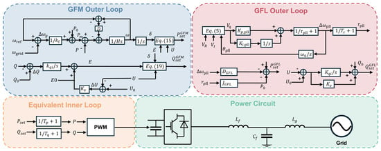
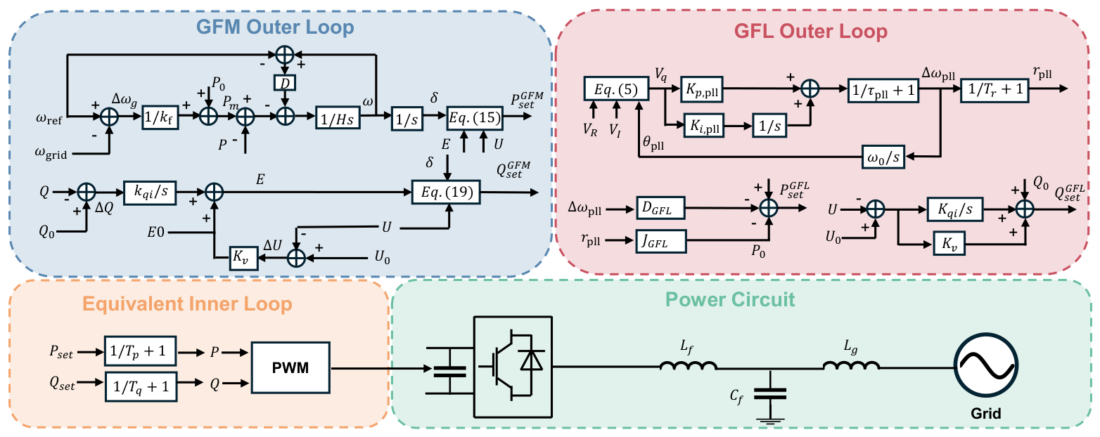
For system-level frequency-response (FR) studies, the converter-interfaced resource is represented as a reduced-order nodal current-injection model to balance response accuracy and simulation efficiency [22,23,24]. Fast current-control dynamics, pulse-width modulation (PWM), and switching processes are not explicitly modeled. As shown in Figure 1, the GFM and GFL converters adopt different outer-loop synchronization and power-command generation mechanisms, while both control modes generate active- and reactive-power commands for a common equivalent inner loop. The inner-loop control commands are sent to PWM and then applied to the converter power circuit. In this paper, this fast control path is simplified as first-order active- and reactive-power tracking dynamics. The converter is connected to the grid through an LCL filter, where , , and denote the converter-side filter inductor, filter capacitor, and grid-side filter inductor, respectively.
Figure 1.
Reduced-order equivalent control structure and power circuit of grid-forming and grid-following converters.
The applicability of reduced-order converter models depends on the time scale and dynamic phenomena of interest. Misyris et al. showed that RMS representations can be suitable for grid-forming converter frequency-support studies when sufficient time-scale separation exists [25], while Vorobev et al. noted that neglected fast dynamics may affect stability boundaries in some conditions [26]. Therefore, the present model is intended for system-level electromechanical FR analysis and does not capture switching-level or detailed inner-loop stability phenomena.
2.1.1. Common Equivalent Inner Loop
For both GFL and GFM converters, the inner loop is represented by first-order active- and reactive-power tracking dynamics [24]. Given the outer-loop power commands and , where , the actual active and reactive powers follow
where and are the active- and reactive-power response time constants, respectively.
2.1.2. GFL Outer Loop
The GFL converter tracks the grid-voltage phase and frequency through a phase-locked loop (PLL). Its frequency-support function is implemented by modulating the active-power command according to the PLL-measured frequency deviation and RoCoF [10,18,27]. The frequency-deviation term provides virtual damping, while the RoCoF-related term provides virtual inertia. Let denote the PLL-estimated frequency. The PLL frequency deviation is defined as
where is the nominal frequency. The PLL phase angle is obtained by integrating the PLL frequency-deviation signal,
where is the nominal angular frequency. The q-axis voltage input of the PLL is expressed as
where and are the real and imaginary components of the terminal voltage, respectively. The PLL frequency-deviation dynamics are represented by
where is the PLL time constant, and and are the proportional and integral gains of the PLL, respectively. Equations (3)–(6) describe the closed-loop PLL dynamics: the PLL frequency-deviation signal determines the phase angle, the phase angle is used to calculate the q-axis voltage, and the q-axis voltage drives the PLL frequency-deviation dynamics. The RoCoF signal is represented by the following first-order filtered-derivative dynamics,
where is the RoCoF filter time constant. The active-power command generated by the GFL outer loop is
where is the initial active-power operating point, is the virtual-inertia coefficient, and is the virtual-damping coefficient associated with the frequency-deviation feedback.
The reactive-power command generated by the GFL outer loop is
where and are the initial reactive-power and voltage operating points, respectively, and and are the integral and proportional voltage-regulation gains.
2.1.3. GFM Outer Loop
The GFM converter forms its internal frequency and voltage phase through self-synchronizing power–angle dynamics [28]. The measured grid-frequency deviation and the converter-side relative frequency deviation are defined as
where is the measured grid frequency and is the internal frequency of the GFM converter.
The mechanical-power-like command is generated by the frequency-droop loop,
where is the active-power limit and is the frequency-droop coefficient.
The internal frequency and power–angle dynamics are described by
where is the virtual-inertia coefficient, is the damping coefficient, P is the measured active power, and is the internal power angle.
The active-power command generated by the GFM outer loop is calculated from the internal voltage phasor,
where E is the internal voltage magnitude, U is the terminal voltage magnitude, and is the virtual reactance.
For the reactive-power–voltage outer loop, the reactive-power and voltage deviations are defined as
where and are the initial reactive-power and voltage operating points, respectively. The internal voltage magnitude is generated by
where is the nominal internal voltage, is the reactive-power integral gain, and is the voltage-regulation coefficient. The reactive-power command generated by the GFM outer loop is:
In summary, the GFL converter generates its active-power command from PLL-based frequency measurements, with and representing its virtual-inertia and virtual-damping coefficients, respectively. The GFM converter forms its internal frequency and phase through swing-equation-like dynamics, with and representing the corresponding virtual-inertia and damping coefficients. Both control modes send their active- and reactive-power commands to the common equivalent inner loop in (1) and (2).
The coupling among multiple converter-interfaced resources is mainly introduced through their shared network connection [29]. For a GFM converter, the active-power output is determined by the power–angle relationship,
where represents the internal voltage phase angle of converter i, denotes the voltage phase angle at the PCC, and are the converter internal voltage magnitude and PCC voltage magnitude, respectively, and represents the equivalent reactance between the converter and the PCC.
The power output of each converter is therefore affected by the PCC voltage magnitude and phase angle, which are jointly determined by the responses of all the connected converters and the upstream network.
The internal frequency dynamics of each GFM converter can be expressed as
where represents the relative frequency deviation of converter i.
Therefore, the virtual-inertia coefficient affects not only the local frequency response but also the active-power exchange through the shared network angle. When multiple converters participate in frequency support, changes in one converter’s dynamic response modify the common voltage angle and power distribution, thereby influencing the responses of other converters. Consequently, virtual-inertia coordination cannot be formulated as independent tuning of individual converters because the feasible inertia range of one converter is affected by the dynamic responses of other converters through the shared network.
2.2. Frequency-Support Performance and Dynamic Feasibility
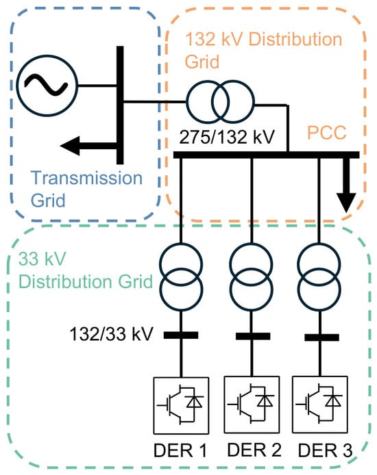
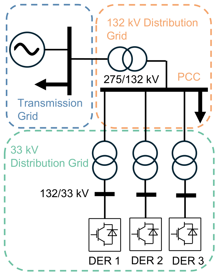
To illustrate the converter-dynamic-dependent frequency-support characteristics and dynamic-feasibility limitations, two tests are conducted. In the single-DER control-mode comparison, the GFM and GFL converters are assigned the same virtual-inertia and damping coefficients, i.e., s and p.u. A simplified transmission–distribution system is constructed according to typical voltage levels in the United Kingdom electricity network [30]. As shown in Figure 2, a 275 kV upstream grid is connected to a 132 kV local network and then to a 33 kV distribution grid through 132/33 kV transformers. Three converter-interfaced DERs are installed in the 33 kV grid, each rated at 30 MW with an initial active-power operating point of MW. The 132 kV local load is 100 MW, and a 20 MW step disturbance is applied at s in Power System Analysis Software Package (PSASP), version 7.41.
Figure 2.
Transmission–distribution topology with a 132 kV point of common coupling (PCC) between the transmission grid and the distribution system, where distributed energy resources (DERs) are connected to the 33 kV distribution grid through 132/33 kV transformers.
2.2.1. Converter-Dynamic Effects on Frequency Response
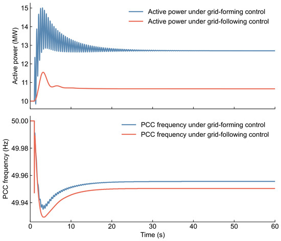
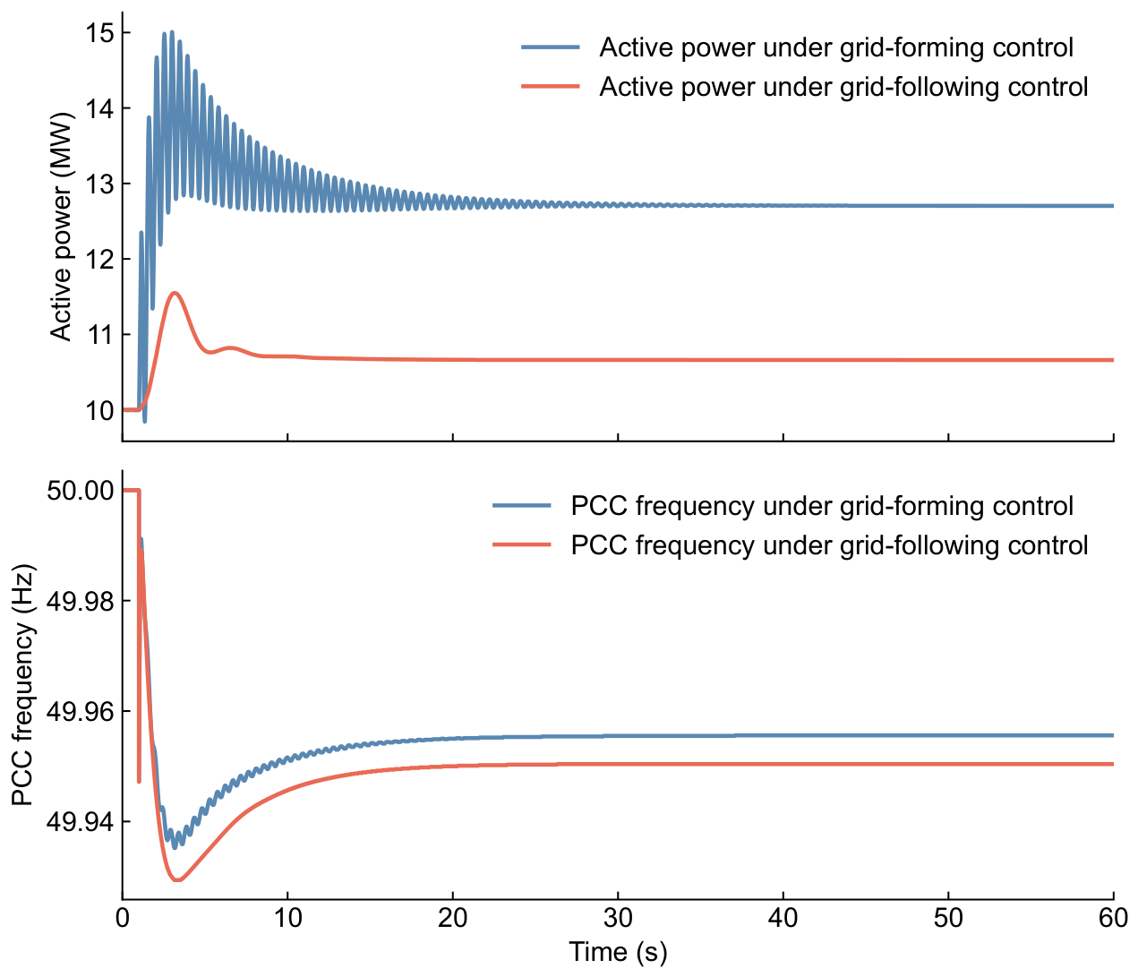
Figure 3 compares the PCC responses obtained when the same DER is operated in GFM and GFL modes. With the same J and D, the GFM-controlled DER reaches a peak active power of about 15.01 MW, whereas the GFL-controlled DER reaches about 11.55 MW. The stronger GFM response reduces the 0.5 s RoCoF magnitude from 0.0630 Hz/s in the GFL case to 0.0524 Hz/s and improves the PCC frequency nadir from about 49.929 Hz to about 49.934 Hz. The GFM active-power response exhibits more pronounced transient oscillations, but these oscillations gradually decay. This indicates that the effective inertia support is affected not only by the assigned inertia coefficient but also the dynamic characteristics of the converter control implementation.
Figure 3.
Point of common coupling (PCC) frequency and active-power responses of the same converter-interfaced source operated under grid-forming (GFM) and grid-following (GFL) control modes.
2.2.2. Dynamic Limits of Multi-Converter Support Considering Converter Coupling Effects
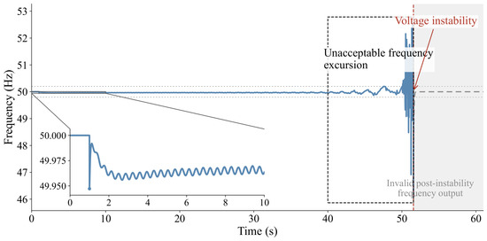
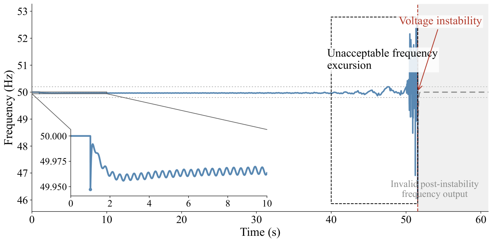
Figure 4 further shows the response when three GFM DERs, each with s and p.u., are connected simultaneously. The initial response appears to be acceptable, with the PCC frequency remaining within approximately 49.947–50.000 Hz during the first 10 s. Nevertheless, the oscillation amplitude begins to increase noticeably after about 40 s, followed by unacceptable frequency excursions and eventual voltage instability at around 50 s. After instability occurs, the apparent return of the simulated frequency to approximately 50 Hz is a nonphysical PSASP output rather than an actual frequency recovery. Thus, a configuration that satisfies the initial RoCoF or nadir requirement may still be dynamically infeasible. This motivates coordinated optimization of GFM and GFL inertia parameters, where converter coupling effects are incorporated through the proposed dynamic-feasibility constraints.
Figure 4.
Dynamic instability at the point of common coupling induced by coupling effects among multiple grid-forming converters, including growing frequency oscillations, voltage instability, and invalid post-instability frequency output.
3. Dynamic-Feasibility-Aware Coordination of Converter-Based Virtual Inertia in Active Distribution Networks
This section develops the proposed dynamic-feasibility-aware coordination method for converter-based virtual inertia in ADNs. First, GPR surrogate models are established to approximate the mappings from virtual-inertia parameters to the initial RoCoF, initial frequency nadir, and post-disturbance feasibility labels. Then, the surrogate predictions are embedded into a normalized weighted RoCoF–nadir optimization model subject to initial frequency-support, full-window security, and dynamic-feasibility constraints. Finally, GMS–SLSQP is developed to solve the resulting surrogate-based nonconvex optimization problem.
3.1. Gaussian Process Regression Surrogate Modeling of Virtual-Inertia-Dependent Performance Metrics
The selected virtual-inertia coefficients, together with the associated damping coefficients determined by (22), affect the PCC frequency and voltage responses through nonlinear-network and converter-control dynamics. However, the mappings from these inertia–damping settings to the post-disturbance response quantities are not available in closed form. Therefore, GPR surrogate models are trained from time-domain simulation samples generated by reduced-order converter models to provide explicit predictions of the initial frequency-support metrics and feasibility indicators for inertia coordination [31,32].
Let be the set of converter-interfaced resources participating in frequency support. Although both the virtual-inertia coefficient and the virtual-damping coefficient enter the converter control models, they are not treated as independent optimization variables in this paper. Following the commonly adopted fixed inertia–damping proportional setting, the damping coefficient is determined from the virtual-inertia coefficient as
where is a given inertia-to-damping ratio [33]. Therefore, the independent decision vector is:
For each candidate , the associated damping coefficients are updated according to (22). The corresponding PCC frequency and voltage responses are denoted by and , respectively.
The response windows are selected to distinguish the immediate frequency-support effect from the subsequent dynamic behavior and are motivated by operational frequency-response assessment practices. The RoCoF window is set to s, following the 500 ms RoCoF calculation interval adopted by EirGrid and SONI [34]. The initial-nadir window is set to s to isolate the immediate virtual-inertia-support stage considered in this study. This 1 s window is consistent with the fast-response time scale represented by the DS3 FFR framework in which the expected response is required within 2 s of the frequency trigger [35]. The full dynamic-feasibility window is set to s so that delayed poorly damped or growing oscillations are not overlooked by short-window frequency metrics. This long-horizon assessment is also consistent with AEMO’s stability-demonstration practice, which requires at least 60 s of recording after the response has settled at its steady-state value [36]. Moreover, the illustrative multi-GFM case in Figure 4 shows that the oscillation amplitude may begin to increase only after approximately 40 s. Let , , and denote the RoCoF-measurement window, the initial-nadir search window, and the dynamic-feasibility evaluation window, respectively. The RoCoF metric is
where is the disturbance time. Since is expressed in Hz, is expressed in Hz/s.
The initial nadir is searched within the initial inertia-support stage:
The metric characterizes the lowest frequency reached during the initial virtual-inertia-support stage and is used as a continuous surrogate-predicted frequency-support metric, while later frequency excursions are separately captured by the full-window extrema over .
The full-window frequency and voltage extrema over are:
These extrema are used to screen unacceptable frequency and voltage excursions during the whole dynamic-feasibility window. Since , captures both the initial frequency dip and any later low-frequency excursion. The full-window extrema are therefore incorporated into the security-feasibility label, while is retained as the continuous metric characterizing the initial virtual-inertia-support stage.
The security-feasibility condition consists of the initial frequency-support requirements and the full-window frequency and voltage limits:
The security-feasibility label is:
Thus, encodes two types of requirements. The RoCoF and initial-nadir constraints evaluate the immediate frequency-support effect during the initial inertia-support stage, whereas the full-window extrema enforce frequency and voltage bounds over the subsequent dynamic process.
To further screen unacceptable tail dynamics, let denote the tail window. For each response signal , the slow trend in is first removed by linear detrending,
where denotes the least-squares linear trend of y over . If the detrended peak-to-peak variation is below Hz for frequency or p.u. for voltage, the corresponding tail signal is regarded as numerically negligible and is directly treated as non-growing, thereby avoiding envelope fitting for essentially flat numerical signals. Otherwise, the oscillation envelope is obtained from the analytic signal,
where denotes the Hilbert transform [37]. The envelope growth rate is estimated by fitting the logarithmic envelope,
where is a small signal-dependent regularization term introduced to avoid taking the logarithm of values close to zero. Only envelope samples satisfying are retained in for fitting. The tail-growth indicator is:
The tail-oscillation label is:
The threshold follows directly from the fitted envelope-growth model: indicates an increasing oscillation amplitude, whereas indicates a non-growing tail response. When the tail oscillation is negligible, is directly set to 1. The overall dynamic-feasibility label is:
Therefore, indicates that the inertia configuration satisfies the initial frequency-support requirements, maintains full-window frequency and voltage security, and does not produce growing tail oscillations.
For each continuous initial frequency-support metric
an independent GPR model is trained:
The predictive mean and standard deviation are:
The simulation-derived binary feasibility labels are mapped to continuous latent targets and modeled using GPR to construct smooth feasibility surfaces for the subsequent nonlinear optimization. The predictive mean and local predictive standard deviation further enable uncertainty-aware feasibility margins to be incorporated directly into the optimization.
The binary feasibility labels are represented by latent functions. For , the latent function is:
A GPR model is trained for each latent function:
Its predictive mean and standard deviation are denoted by and .
For compact notation, and denote the predictive mean and standard deviation of , respectively, whereas and denote those of .
3.2. Dynamic-Feasibility-Aware Inertia Coordination Model for Converter-Based Virtual Inertia
The surrogate models developed in Section 3.1 provide predictions of the initial RoCoF, initial frequency nadir, security-feasibility indicator, and overall dynamic-feasibility indicator. These predictions are embedded into an inertia coordination model that improves the initial frequency-support performance while excluding frequency-insecure, voltage-insecure, and dynamically infeasible inertia settings.
To account for surrogate prediction uncertainty, the robust RoCoF and initial-nadir estimates are defined as
where and control the conservativeness of the uncertainty margins for the RoCoF and initial-nadir predictions, respectively.
The inertia coordination objective is formulated as a normalized weighted combination of the robust RoCoF and initial frequency deviation,
where and are the weights assigned to the RoCoF and initial-nadir terms, respectively, with . The two terms are normalized by their corresponding engineering limits to account for their different units and numerical scales. In this paper, equal weights, i.e., , are adopted to balance RoCoF reduction and initial-nadir improvement [10,38].
The robust initial frequency-support constraints are:
The full-window frequency and voltage limits are imposed through the security-feasibility latent constraint:
Since is generated from (28)–(31), (49) excludes configurations that violate the initial RoCoF and nadir requirements or the full-window frequency and voltage limits. The overall dynamic-feasibility requirement is:
This constraint further excludes configurations with unacceptable tail oscillations or other dynamically infeasible trajectories. The independent virtual-inertia decision variables are bounded by:
Therefore, the feasible region is jointly determined by the robust initial frequency-support constraints, the security-feasibility latent constraint, the dynamic-feasibility latent constraint, and the inertia bounds. Since the GPR mean and uncertainty surfaces are generally nonconvex, a single-start local optimizer may be sensitive to the initial point. GMS–SLSQP is therefore introduced below to combine global grid screening with multi-start local refinement.
3.3. Grid-Assisted Multi-Start Sequential Least-Squares Programming Method
GMS–SLSQP solves the surrogate-based inertia coordination problem by combining grid screening, multi-start initialization, and local SLSQP refinement. The grid scan identifies feasible points with low RoCoF–nadir objective values or, when no feasible grid point exists, points with the smallest aggregate constraint violations for local-search initialization. Representative grid points are selected as initial points using a quality- and diversity-based multi-start strategy for nonconvex optimization [39] and are subsequently refined using SLSQP [40]. The procedure is summarized in Algorithm 1.
The distinguishing feature of GMS–SLSQP is that the surrogate-predicted feasible-region structure is explicitly used to guide local-search initialization. Unlike a generic multi-start scheme in which starting points may be selected independently of the constraints, the proposed method constructs its candidate pool using the surrogate-predicted feasibility and objective information and then selects spatially diverse high-quality starting points for local refinement. In this way, the grid-screening and multi-start stages are directly coupled through the learned converter-dependent feasible region.
Since is determined by through (22), the grid search is performed only over the independent virtual-inertia variables:
For each grid point, the main constraint margins are:
The inertia-bound margins are:
Let denote the set of all the constraint margins. A grid point is surrogate-feasible if:
For an infeasible grid point, the total constraint violation is measured by:
| Algorithm 1 GMS–SLSQP for Dynamic-Feasibility-Aware Inertia Coordination |
|
After the grid scan, candidate initial points are selected according to both quality and diversity. If feasible grid points exist, the candidate pool is formed from feasible points with smaller weighted RoCoF–nadir objective values; otherwise, it is formed from points with smaller total violations. Let denote the normalized coordinate of in the inertia space. For a candidate , the diversity-aware selection score is
where is the set of selected initial points, is the ranking-based quality score, and and are the diversity and quality weights, respectively. The next initial point is selected as:
Starting from each selected initial point, local SLSQP solves:
The feasible refined solutions form the set , from which the final surrogate optimum is selected as:
4. Case Studies
4.1. Settings
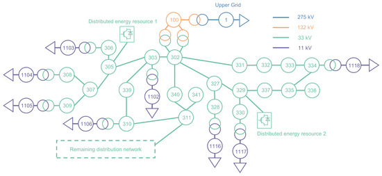
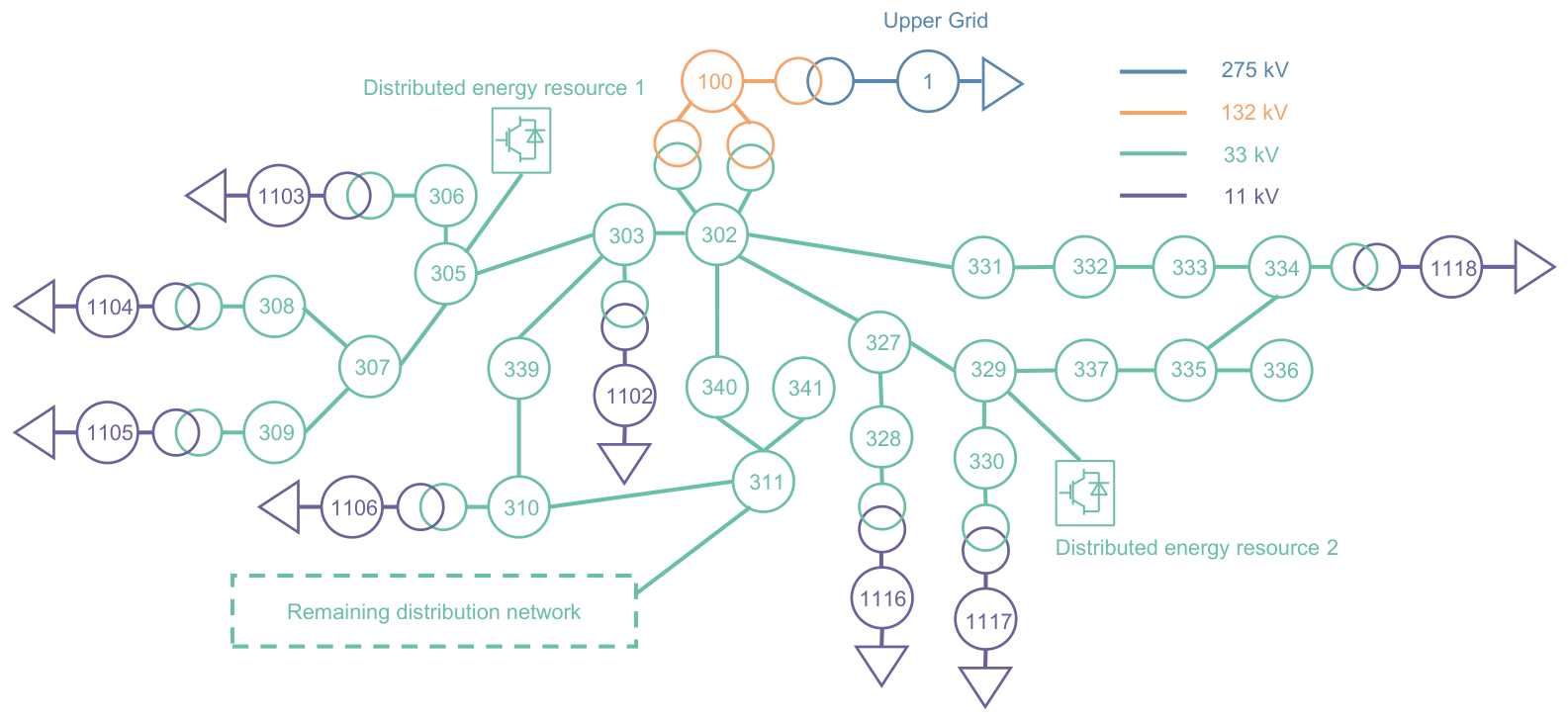
The proposed method is evaluated on a modified United Kingdom Generic Distribution System (UKGDS) EHV1 active distribution network [41], as shown in Figure 5. Two converter-interfaced DERs are connected at the 33 kV Buses 305 and 329, each with an initial active-power output of MW. The system base is MVA.
Figure 5.
Modified UKGDS EHV1 topology with two distributed energy resources connected at Buses 305 and 329.
Three converter-dynamic configurations are considered to investigate how converter-dynamic composition affects the attainable frequency-support performance and virtual-inertia allocation. Configuration I assigns the DERs at Buses 305 and 329 as GFM and GFL, respectively; Configuration II operates both DERs in GFM mode; and Configuration III operates both DERs in GFL mode. Under each configuration, three inertia-setting methods are evaluated. Method I is the proposed dynamic-feasibility-aware coordination method. It minimizes a normalized weighted objective constructed from the robust RoCoF and initial-nadir metrics, where the two terms are normalized by their respective engineering limits and assigned equal weights, i.e., [10,38]. The optimization is subject to the frequency-security and dynamic-feasibility constraints formulated in Section 3. Method II is a frequency-performance-oriented optimization benchmark that employs the same objective, parameter bounds, and robust initial-frequency constraints as Method I but omits the latent constraints associated with full-window frequency and voltage security and tail dynamics. Method III sets the parameters directly to their upper limits, i.e., s and p.u., and serves as the maximum-inertia benchmark.
A 20 MW step load disturbance is applied at Bus 1 of the upstream 275 kV grid at s, and the post-disturbance dynamics are simulated for 60 s using the reduced-order converter models implemented in PSASP. The PCC frequency and voltage are monitored at the 132 kV Bus 100. RoCoF is evaluated over the first s, the initial nadir is searched within s, and the full security window is s, following the window definitions and rationale given in Section 3.1. The baseline tail-analysis window is set to s so that the oscillation indicator focuses on the late-stage response after the initial frequency-support transient. To assess the sensitivity to this modeling choice, the starting point of the tail window is additionally varied to 35 s and 45 s after the disturbance while retaining the same 60 s endpoint. The limits are 0.5 Hz/s for RoCoF, 49.8–50.2 Hz for PCC frequency, and 0.9–1.1 p.u. for PCC voltage [42,43]. Table 1 lists the main control and optimization parameters.
Table 1.
Key parameters used in case studies.
For all three converter-control configurations, the GPR surrogates use an anisotropic radial basis function (RBF) covariance with an additive white-noise term. The signal variance is initialized at 1.0 and optimized over . The length scale for each inertia-input dimension is initialized at 1.0 and optimized over , allowing anisotropic sensitivity across the input dimensions. The noise variance is initialized at and optimized over , corresponding to independent homoscedastic residual noise. The inertia inputs are standardized to zero mean and unit variance, while the target values are normalized during model fitting. All the covariance hyperparameters are estimated by maximizing the log marginal likelihood using 10 optimizer restarts with a fixed random state of 42. The continuous RoCoF and initial-nadir surrogates are trained using numerically valid stable trajectories, whereas all the training samples are retained for the latent feasibility surrogates.
4.2. Surrogate Accuracy and Dynamic-Feasibility Region
For each converter-control configuration, 53 time-domain simulation cases were used for surrogate training, with the same sampling locations in the – space used for all three configurations. An independent validation set of 30 nontraining cases was constructed for each configuration, comprising 20 hold-out cases and 10 boundary-focused cases. The exact training, hold-out, and boundary-focused sampling locations are reported in Appendix A. The trained models were subsequently evaluated over the grid without performing additional time-domain simulations during grid screening.
The 10 boundary-focused cases were selected from previously unsimulated locations close to the surrogate-predicted zero-margin boundary before their time-domain feasibility outcomes were known, and none of these cases was used for surrogate training. Therefore, they provide an independent challenge set for evaluating the learned feasibility boundary. For the classification assessment, a dynamically feasible case is defined as the positive class. Accordingly, true positive (TP) denotes an actually feasible case correctly predicted as feasible, true negative (TN) denotes an actually infeasible case correctly predicted as infeasible, false positive (FP) denotes an actually infeasible case incorrectly predicted as feasible, and false negative (FN) denotes an actually feasible case incorrectly predicted as infeasible. The false-positive rate (FPR) and false-negative rate (FNR) are also reported to quantify the two types of classification errors.
As shown in Table 2, the continuous RoCoF and 1 s initial-nadir surrogates retain low RMSE values and values close to unity on the validation set. The continuous-metric errors are evaluated using numerically valid stable trajectories; consequently, 30, 29, and 30 cases are available for the continuous metrics in Configurations I–III, respectively. For dynamic-feasibility classification, the accuracies over the complete 30-case validation sets are 0.833, 0.767, and 0.833, with TP/TN/FP/FN counts of 23/2/0/5, 9/14/0/7, and 5/20/0/5 for Configurations I–III, respectively. Notably, no false-positive, i.e., false-feasible, prediction is observed in any configuration, and the corresponding FPR remains zero.
Table 2.
Prediction performance of the frequency-metric GPR surrogates and dynamic-feasibility latent GP on the 30-case validation set.
Table 3 presents the confusion matrices of the dynamic-feasibility predictions. For Configurations I–III, respectively, the 30-case validation sets contain 23, nine, and five TPs; two, 14, and 20 TNs; no FPs; and five, seven, and five FNs. Therefore, no dynamically infeasible case is incorrectly classified as feasible in any of the three configurations. In contrast, all the observed classification errors correspond to feasible cases being conservatively classified as infeasible. For the 10 boundary-focused cases, the time-domain simulations identified all the cases as dynamically feasible in each configuration. The surrogate correctly accepted eight, five, and five of these cases in Configurations I–III, respectively, while two, five, and five cases were conservatively classified as infeasible. Therefore, the boundary-focused subsets contain TP/FN counts of 8/2, 5/5, and 5/5 for Configurations I–III, respectively. These results show that the surrogate becomes more conservative close to the learned feasibility boundary, with the observed boundary errors corresponding to feasible settings being rejected rather than dynamically infeasible settings being accepted.
Table 3.
Confusion matrices of the dynamic-feasibility latent GP on the 30-case validation sets.
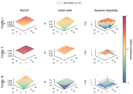
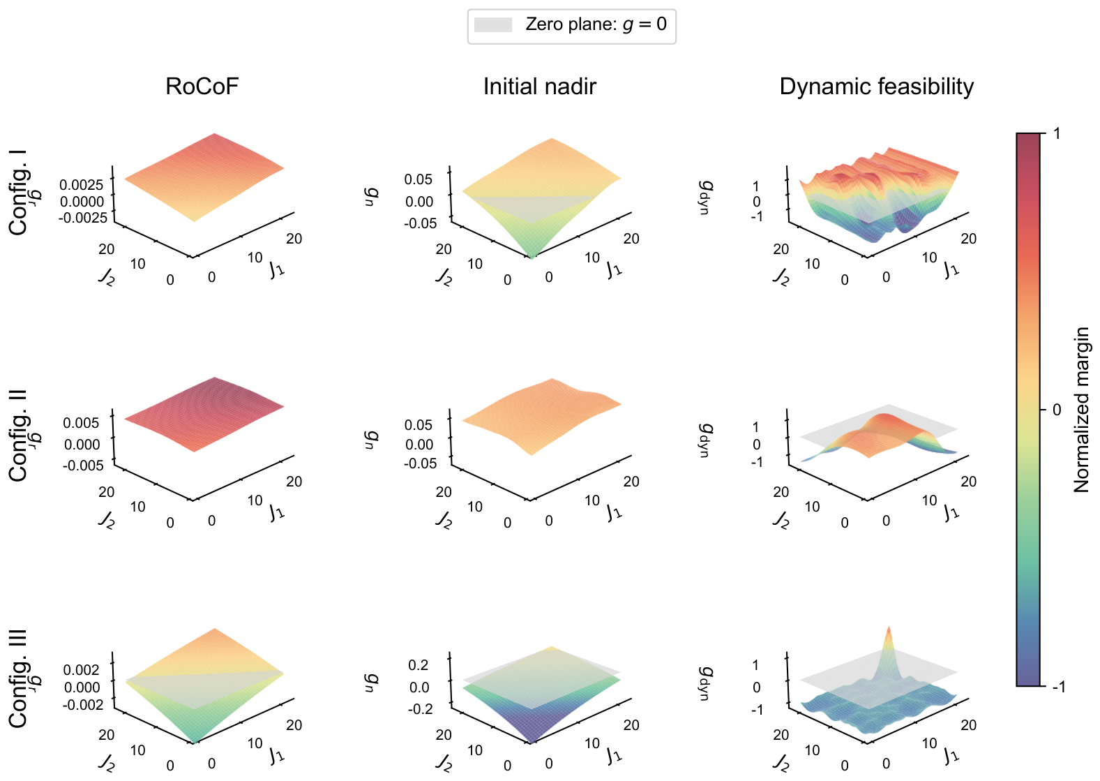
Figure 6 presents the surrogate-predicted constraint margins over the screening grid, where a nonnegative margin indicates constraint satisfaction. In Configuration I, the RoCoF constraint is satisfied throughout the grid, while 68.3% and 64.3% of the points satisfy the initial-nadir and dynamic-feasibility requirements, respectively, resulting in a jointly feasible ratio of 62.7%. The upper-inertia region remains feasible, indicating that improved initial frequency performance does not conflict with dynamic feasibility in the mixed GFM/GFL configuration. In Configuration II, both initial-frequency constraints are satisfied throughout the grid, but the dynamic-feasibility requirement reduces the jointly feasible ratio to 51.0% by excluding part of the high-inertia region. This reveals that the strong initial support provided by multiple GFM resources may conceal unacceptable subsequent dynamics. Configuration III is instead limited mainly by insufficient initial support: only 43.2% and 0.9% of the grid satisfy the RoCoF and initial-nadir requirements, respectively, leaving a jointly feasible ratio of 0.5% near the upper inertia bounds. These results show that the dominant limiting factor depends on the control-mode composition: dynamic feasibility limits the all-GFM configuration, whereas initial frequency-support performance limits the all-GFL configuration.
Figure 6.
Surrogate-predicted RoCoF, initial-nadir, and dynamic-feasibility margins in the – space, where and denote the virtual-inertia coefficients of the DERs at Buses 305 and 329. The gray plane represents the zero-margin boundary.
4.3. Virtual-Inertia Configuration Results
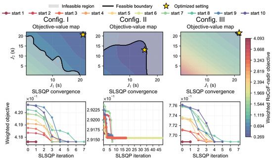
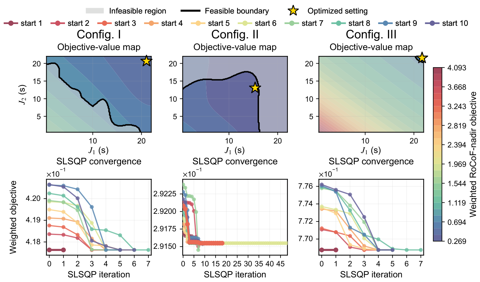
Figure 7 and Table 4 present the search processes and inertia settings obtained by the three methods. In Configurations I and III, the weighted RoCoF–nadir objective decreases toward the upper inertia bounds, which remain dynamically feasible; therefore, all three methods select s. This indicates that the proposed constraints do not modify the solution when the frequency-performance optimum is already dynamically feasible. The all-GFM Configuration II exhibits the key performance–feasibility conflict: although the objective continues to improve with increasing inertia coefficients, the lower-objective region extends beyond the dynamic-feasibility boundary. Consequently, Method II, which omits the full-window security and dynamic-feasibility constraints, selects s, close to the maximum-inertia setting s of Method III, whereas Method I converges to s within the dynamically feasible region. Under Method I, the normalized objective values are 0.41763, 0.29155, and 0.76876 for Configurations I–III, respectively, with robust RoCoF values of 0.275, 0.207, and 0.387 Hz/s and robust initial nadirs of 49.854, 49.872, and 49.806 Hz. Thus, the proposed method preserves comparable initial frequency-support performance while preventing the optimizer from selecting high-inertia settings that lead to sustained oscillations and full-window frequency-limit violations.
Figure 7.
Weighted RoCoF–nadir objective maps and GMS–SLSQP search trajectories of the proposed dynamic-feasibility-aware coordination method (Method I) under different converter-control configurations.
Table 4.
Virtual-inertia settings obtained by the three methods and surrogate-level results of Method I.
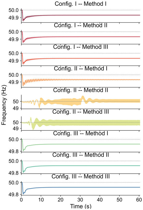
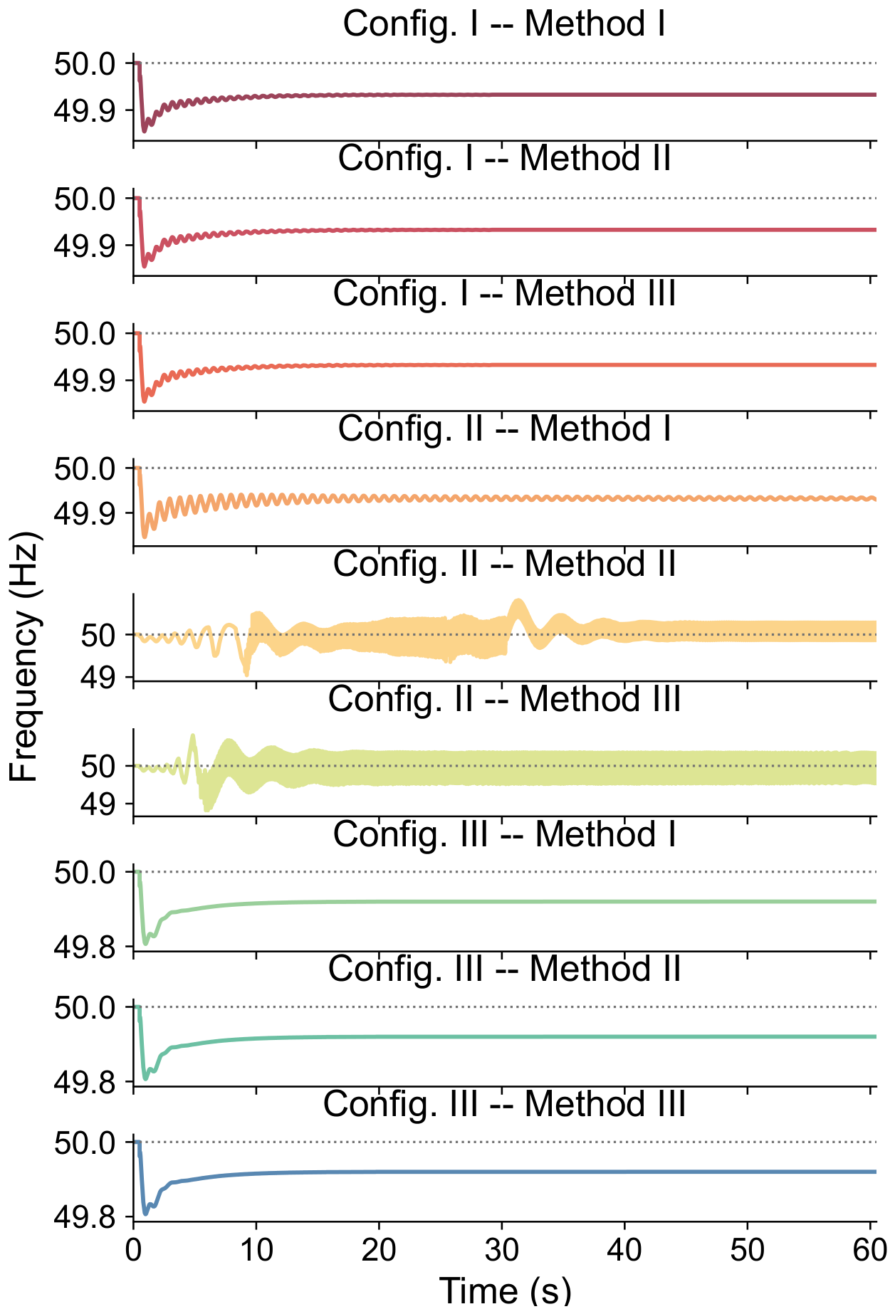
Figure 8 compares the PCC frequency responses obtained by re-simulating the selected settings in the PSASP model. In Configurations I and III, all three methods select s and consequently produce identical frequency-secure responses, confirming that the proposed constraints do not unnecessarily alter the solution when the performance-oriented optimum is already dynamically feasible. The decisive difference appears in the all-GFM Configuration II. Method I with s and Method II with s achieve almost identical initial responses, with RoCoF values of 0.293 and 0.293 Hz/s and initial nadirs of 49.846 and 49.843 Hz, respectively. However, Method II subsequently develops sustained oscillations, causing the PCC frequency to vary between 49.043 and 50.810 Hz and thereby violate both the lower and upper limits of the prescribed 49.8–50.2 Hz security range. Method III improves the initial RoCoF and nadir to 0.170 Hz/s and 49.870 Hz but produces an even wider frequency range of 48.822–50.811 Hz, again violating both frequency limits. In contrast, Method I maintains the PCC frequency within 49.846–50.000 Hz and yields a stable post-disturbance response. Since Methods I and II employ the same RoCoF–nadir objective, these results demonstrate that the proposed full-window security and dynamic-feasibility constraints preserve comparable initial frequency support while excluding settings with insecure full-window responses.
Figure 8.
PCC frequency responses under different converter-control configurations and coordination methods.
Table 5 examines the sensitivity to the tail-analysis window by shifting its starting point from the baseline 40 s to 35 s and 45 s after the disturbance while retaining the same 60 s endpoint. The agreement rate is defined as the percentage of samples whose dynamic-feasibility label remains identical to that obtained using the baseline 40–60 s window. For all three converter-control configurations, both the training and test sets achieve 100% agreement for the two alternative windows. The resulting Method I optimal inertia settings also remain unchanged: s for Configurations I and III and s for Configuration II. These results indicate that the feasibility classification and the resulting inertia-coordination solution are insensitive to moderate variations in the selected tail-analysis window.
Table 5.
Sensitivity of the dynamic-feasibility assessment and optimized inertia settings to the tail-analysis window.
4.4. Sensitivity Analysis of the Inertia–Damping Ratio
To investigate the effect of the imposed inertia–damping relationship , a sensitivity analysis is conducted for all three converter-control configurations. The virtual-inertia coefficients are fixed at the Method I optimal settings: s for Configuration I, s for Configuration II, and s for Configuration III. A common ratio is varied over , and the corresponding damping coefficients are recalculated according to . Each setting is re-simulated in the PSASP model under the same 20 MW disturbance without repeating the optimization.
As shown in Table 6, increasing R reduces the associated damping coefficients and consistently degrades the initial frequency response: the RoCoF increases and the initial nadir decreases in all three configurations. Configurations I and II remain frequency-secure over the tested range, although Configuration II shows an increase in the 40–60 s frequency peak-to-peak variation from 0.0004 to 0.0023 Hz as the damping is reduced. Configuration III is more sensitive to the inertia–damping ratio: its initial nadir decreases from 49.8216 Hz at to 49.7936 Hz at , and the cases with and violate the 49.8 Hz lower frequency limit. The PCC voltage remains within the prescribed limits for all the tested cases. These results confirm that the assumed inertia–damping ratio affects the quantitative frequency response and may change the feasibility assessment when the operating point is close to a security boundary.
Table 6.
Sensitivity of frequency-support performance to the inertia–damping ratio under the Method I optimal inertia settings.
4.5. Robustness Validation Under Disturbance Variations
To further evaluate the out-of-sample robustness of the optimized inertia settings, the Method I solutions obtained under the nominal MW load disturbance are directly re-simulated under two additional disturbances without retraining the surrogate models or repeating the optimization. Specifically, a MW load increase, representing a 50% increase in disturbance magnitude, and a reverse MW load disturbance are considered. All the other system and control parameters are kept unchanged. For the load-increase cases, the initial frequency extremum corresponds to the nadir, whereas, for the load-decrease case, it corresponds to the initial frequency peak.
As shown in Table 7, Configuration II exhibits the strongest disturbance robustness. The optimized all-GFM setting remains feasible under both additional disturbances. Even when the load increase is enlarged by 50% to 30 MW, the RoCoF remains at 0.2926 Hz/s and the minimum frequency remains at 49.8072 Hz. The two GFM DERs also provide relatively coordinated active-power support, with their outputs increasing from approximately 10 MW to 30.000 and 29.304 MW, respectively. Under the reverse MW disturbance, both GFM units reduce their active-power outputs and the PCC frequency remains within the prescribed limits. Configuration I remains feasible for the reverse disturbance, but the MW stress case exceeds its robustness margin. In this case, the GFM DER output spans to 30 MW while the GFL DER reaches 30 MW, accompanied by a large full-window frequency excursion of 49.2176–50.1304 Hz and a tail peak-to-peak variation of 0.4588 Hz. Configuration III remains essentially non-oscillatory, but its frequency-support margin is smaller: under MW, the two GFL DERs increase only to 25.629 and 25.244 MW, and the RoCoF and frequency nadir violate their limits. Under MW, the maximum frequency reaches 50.2011 Hz, marginally exceeding the 50.2 Hz limit. The PCC voltage remains within the prescribed range in all the tested cases. Overall, the results demonstrate configuration-dependent robustness margins, with the optimized all-GFM configuration showing the strongest adaptability to changes in disturbance magnitude and direction.
Table 7.
Robustness validation of the Method I optimal settings under additional load disturbances.
5. Conclusions
This paper proposed a dynamic-feasibility-aware coordination method for converter-based virtual inertia in ADNs. GPR surrogates trained using electromechanical-transient simulation data were developed to predict the initial RoCoF and initial frequency nadir and to screen full-window security and tail-oscillation behavior. These surrogates were incorporated into a normalized weighted RoCoF–nadir optimization model, and the resulting nonconvex problem was solved using GMS–SLSQP.
Case studies showed that the attainable frequency-support performance and admissible inertia settings depend strongly on the GFM/GFL composition. In the mixed GFM/GFL configuration, the upper-inertia region remained dynamically feasible, whereas the all-GFL configuration was mainly limited by insufficient initial frequency support. In the all-GFM configuration, frequency-performance-oriented optimization achieved nearly the same initial RoCoF and nadir as the proposed method but subsequently produced sustained oscillations and frequency-limit violations, whereas the proposed method maintained the PCC frequency within 49.846–50.000 Hz and achieved a stable post-disturbance response. The sensitivity analyses further showed that the optimized settings are insensitive to moderate variations in the tail-analysis window, while reduced damping may degrade frequency performance and alter feasibility near security boundaries. Additional disturbance tests revealed configuration-dependent robustness margins, with the optimized all-GFM setting remaining feasible under both a 50% larger load increase and a reverse load disturbance. These results confirm that virtual-inertia coordination should account for full-window dynamic feasibility rather than relying only on initial frequency metrics.
Although two DERs are used in the present case study for clear visualization of the feasible region, the formulation can be extended to more converter-interfaced resources. The main scalability limitation arises from the dense grid screening, whose number of points grows as for independent inertia variables, together with the training complexity of standard GPR. For larger converter populations, adaptive sampling or sparse GPR can be employed to reduce the computational burden, which will be investigated in future work.
Author Contributions
Conceptualization, T.Y.; methodology, T.Y.; software, T.Y.; validation, T.Y.; formal analysis, T.Y. and M.M.; writing—original draft preparation, T.Y.; writing—review and editing, T.Y. and H.L.; supervision, H.L., C.Y. and J.Z.; project administration, C.Y. and J.Z.; funding acquisition, C.Y. and J.Z. All authors have read and agreed to the published version of the manuscript.
Funding
This research was funded by the National Natural Science Foundation of China, grant number 72331009; the Science Research Project of Hebei Education Department, grant number QN2026646; and the Shenzhen Key Lab of Crowd Intelligence Empowered Low-Carbon Energy Network, grant number ZDSYS20220606100601002.
Institutional Review Board Statement
Not applicable.
Informed Consent Statement
Not applicable.
Data Availability Statement
The data presented in this study are available on request from the corresponding author.
Conflicts of Interest
The authors declare no conflicts of interest.
Appendix A. Surrogate Training and Validation Sampling Points
For reproducibility, the inertia sampling locations used for surrogate training and validation are reported below. The same 53 training locations and 20 hold-out validation locations in the – space are used for all three converter-control configurations. Here, and denote the virtual-inertia coefficients of the DERs at Buses 305 and 329, respectively. The 10 boundary-focused validation locations are selected separately for each configuration because the predicted feasibility boundary depends on the converter-control composition.
Table A1.
Virtual-inertia settings of the 53 surrogate-training cases used in all three converter-control configurations.
Table A2.
Virtual-inertia settings of the 20 hold-out validation cases used in all three converter-control configurations.
Table A3.
Virtual-inertia settings of the 10 boundary-focused validation cases for each converter-control configuration.
References
- Australian Energy Market Operator. 2023 Inertia Report: A Report for the National Electricity Market; Technical report; Australian Energy Market Operator: Melbourne, Australia, 2023. [Google Scholar]
- Khan, S.A.; Wang, M.; Su, W.; Liu, G.; Chaturvedi, S. Grid-Forming Converters for Stability Issues in Future Power Grids. Energies 2022, 15, 4937. [Google Scholar] [CrossRef] [Scilit]
- Panel, I.I.E. Continental Europe Synchronous Area Separation on 08 January 2021-Final Report. Expert Panel Sep. Cont. Eur. Synchronous Area 2021, 8, 66. [Google Scholar]
- Baviskar, A.; Das, K.; Koivisto, M.; Hansen, A.D. Multi-Voltage Level Active Distribution Network With Large Share of Weather-Dependent Generation. IEEE Trans. Power Syst. 2022, 37, 4874–4884. [Google Scholar] [CrossRef] [Scilit]
- Kontis, E.O.; Nozal, A.R.d.; Mauricio, J.M.; Demoulias, C.S. Provision of Primary Frequency Response as Ancillary Service From Active Distribution Networks to the Transmission System. IEEE Trans. Smart Grid 2021, 12, 4971–4982. [Google Scholar] [CrossRef] [Scilit]
- Fuchs, A.; Demiray, T.; Larsson, M. Aggregated models of active distribution networks for stability studies of large transmission systems. Electr. Power Syst. Res. 2022, 212, 108607. [Google Scholar] [CrossRef] [Scilit]
- Li, Y.; Gu, Y.; Green, T.C. Revisiting Grid-Forming and Grid-Following Inverters: A Duality Theory. IEEE Trans. Power Syst. 2022, 37, 4541–4554. [Google Scholar] [CrossRef] [Scilit]
- Ducoin, E.A.S.; Gu, Y.; Chaudhuri, B.; Green, T.C. Analytical Design of Contributions of Grid-Forming and Grid-Following Inverters to Frequency Stability. IEEE Trans. Power Syst. 2024, 39, 6345–6358. [Google Scholar] [CrossRef] [Scilit]
- Orihara, D.; Kikusato, H.; Hashimoto, J.; Otani, K.; Takamatsu, T.; Oozeki, T.; Taoka, H.; Matsuura, T.; Miyazaki, S.; Hamada, H.; et al. Contribution of Voltage Support Function to Virtual Inertia Control Performance of Inverter-Based Resource in Frequency Stability. Energies 2021, 14, 4220. [Google Scholar] [CrossRef] [Scilit]
- Poolla, B.K.; Groß, D.; Dörfler, F. Placement and implementation of grid-forming and grid-following virtual inertia and fast frequency response. IEEE Trans. Power Syst. 2019, 34, 3035–3046. [Google Scholar] [CrossRef] [Scilit]
- Struwe, J.; Wrede, H.; Vennegeerts, H. Validation Aspects for Grid-Forming Converters Based on System Characteristics and Inertia Impact. Energies 2023, 16, 7357. [Google Scholar] [CrossRef] [Scilit]
- Ahmed, M.; Alsokhiry, F.; Abdel-Khalik, A.S.; Ahmed, K.H.; Al-Turki, Y. Improved Damping Control Method for Grid-Forming Converters Using LQR and Optimally Weighted Feedback Control Loops. IEEE Access 2021, 9, 87484–87500. [Google Scholar] [CrossRef] [Scilit]
- Zhao, F.; Zhu, T.; Li, Z.; Wang, X. Low-Frequency Resonances in Grid-Forming Converters: Causes and Damping Control. IEEE Trans. Power Electron. 2024, 39, 14430–14447. [Google Scholar] [CrossRef] [Scilit]
- Sun, P.; Xu, H.; Yao, J.; Chi, Y.; Huang, S.; Cao, J. Dynamic Interaction Analysis and Damping Control Strategy of Hybrid System With Grid-Forming and Grid-Following Control Modes. IEEE Trans. Energy Convers. 2023, 38, 1639–1649. [Google Scholar] [CrossRef] [Scilit]
- Makolo, P.; Zamora, R.; Perera, U.; Lie, T.T. Flexible Synthetic Inertia Optimization in Modern Power Systems. Inventions 2024, 9, 18. [Google Scholar] [CrossRef] [Scilit]
- Zhao, X.; Wen, R.; Mo, W. Optimal Configuration of Virtual Inertia and Fast Frequency Response in Low-Inertia Power Systems. Energies 2026, 19, 1848. [Google Scholar] [CrossRef] [Scilit]
- Nozal, Á.R.d.; Kontis, E.O.; Mauricio, J.M.; Demoulias, C.S. Provision of inertial response as ancillary service from active distribution networks to the transmission system. IET Gener. Transm. Distrib. 2020, 14, 5123–5134. [Google Scholar] [CrossRef] [Scilit]
- Yu, H.; Yao, L.; Liang, S.; Xu, J.; Cheng, F.; Wu, M. Coordinated control of grid-following and grid-forming energy storage for virtual inertia response considering frequency modal characteristics. Int. J. Electr. Power Energy Syst. 2025, 168, 110686. [Google Scholar] [CrossRef] [Scilit]
- Kerdphol, T.; Rahman, F.S.; Mitani, Y.; Hongesombut, K.; Küfeoğlu, S. Virtual inertia control-based model predictive control for microgrid frequency stabilization considering high renewable energy integration. Sustainability 2017, 9, 773. [Google Scholar] [CrossRef] [Scilit]
- Fu, S.; Sun, Y.; Li, L.; Liu, Z.; Han, H.; Su, M. Power Oscillation Suppression in Multi-VSG Grid by Adaptive Virtual Impedance Control. IEEE Syst. J. 2022, 16, 4744–4755. [Google Scholar] [CrossRef] [Scilit]
- Li, J.; Shi, R.; Dong, Z.; Li, J.; Zhang, X. Power-frequency oscillation modeling, analysis and suppression of multi-VSG grid-connected system. Int. J. Electr. Power Energy Syst. 2025, 172, 111129. [Google Scholar] [CrossRef] [Scilit]
- He, P.; Li, Z.; Jin, H.; Zhao, C.; Fan, J.; Wu, X. An adaptive VSG control strategy of battery energy storage system for power system frequency stability enhancement. Int. J. Electr. Power Energy Syst. 2023, 149, 109039. [Google Scholar] [CrossRef] [Scilit]
- Qin, X.; Su, L.; Chi, Y.; Guo, Q.; Xu, X. Functional Orientation Discrimination of Inertia Support and Primary Frequency Regulation of Virtual Synchronous Generator in Large Power Grid. Autom. Electr. Power Syst. 2018, 42, 36–43. (In Chinese) [Google Scholar] [CrossRef]
- Li, Y.; Jing, P.; Wang, L.; Xu, Y.; Yang, Z.; Zhang, B.; Mao, C. A Mathematical Model of Versatile Energy Storage System and Its Modeling by Power System Analysis Software Package. Power Syst. Technol. 2012, 36, 51–57. [Google Scholar] [CrossRef]
- Misyris, G.S.; Chatzivasileiadis, S.; Weckesser, T. Grid-forming converters: Sufficient conditions for RMS modeling. Electr. Power Syst. Res. 2021, 197, 107324. [Google Scholar] [CrossRef] [Scilit]
- Vorobev, P.; Huang, P.H.; Al Hosani, M.; Kirtley, J.L.; Turitsyn, K. High-fidelity model order reduction for microgrids stability assessment. IEEE Trans. Power Syst. 2017, 33, 874–887. [Google Scholar] [CrossRef] [Scilit]
- Guo, X.; Zhu, D.; Hu, J.; Zou, X.; Kang, Y.; Guerrero, J.M. Inertial PLL of grid-connected converter for fast frequency support. CSEE J. Power Energy Syst. 2022, 9, 1594–1599. [Google Scholar] [CrossRef] [Scilit]
- Guo, L.; Xu, Z.; Jin, N.; Li, Y.; Wang, W. A weighted voltage model predictive control method for a virtual synchronous generator with enhanced parameter robustness. Prot. Control Mod. Power Syst. 2021, 6, 38. [Google Scholar] [CrossRef] [Scilit]
- Thilekha, T.; Filizadeh, S.; Annakkage, U.; Karawita, C.; Muthumuni, D. Analysis of interactions among parallel grid-forming inverters. Electr. Power Syst. Res. 2023, 223, 109652. [Google Scholar] [CrossRef] [Scilit]
- Department for Business, Energy & Industrial Strategy. Electricity Networks Strategic Framework: Appendix 1—Electricity Networks Modelling; GOV.UK: London, UK, 2022.
- Williams, C.K.; Rasmussen, C.E. Gaussian Processes for Machine Learning; MIT Press: Cambridge, MA, USA, 2006; Volume 2. [Google Scholar]
- Tan, B.; Su, T.; Weng, Y.; Ye, K.; Pareek, P.; Vorobev, P.; Nguyen, H.; Zhao, J.; Deka, D. Gaussian processes in power systems: Techniques, applications, and future works. Appl. Energy 2026, 402, 126995. [Google Scholar] [CrossRef] [Scilit]
- Tuo, M.; Li, X. Security-Constrained Unit Commitment Considering Locational Frequency Stability in Low-Inertia Power Grids. IEEE Trans. Power Syst. 2023, 38, 4134–4147. [Google Scholar] [CrossRef] [Scilit]
- EirGrid; SONI. RoCoF Alternative & Complementary Solutions Project: Phase 2 Study Report; Technical report; EirGrid: Dublin, Ireland; SONI: Belfast, Ireland, 2015. [Google Scholar]
- EirGrid; SONI. DS3 System Services Protocol–Regulated Arrangements; Protocol document; EirGrid: Dublin, Ireland; SONI: Belfast, Ireland, 2022. [Google Scholar]
- Australian Energy Market Operator. Primary Frequency Response Requirements; Technical report; Australian Energy Market Operator: Melbourne, Australia, 2024. [Google Scholar]
- Cohen, L. Time-Frequency Analysis; Prentice Hall Signal Processing Series; Prentice Hall PTR: Englewood Cliffs, NJ, USA, 1995; p. 299. [Google Scholar]
- Tamrakar, U.; Hansen, T.M.; Tonkoski, R.; Copp, D.A. Model Predictive Frequency Control of Low Inertia Microgrids. In Proceedings of the 2019 IEEE 28th International Symposium on Industrial Electronics (ISIE), Vancouver, BC, Canada, 12–14 June 2019; pp. 2111–2116. [Google Scholar] [CrossRef] [Scilit]
- Rinnooy Kan, A.; Timmer, G.T. Stochastic global optimization methods part I: Clustering methods. Math. Program. 1987, 39, 27–56. [Google Scholar] [CrossRef] [Scilit]
- Kraft, D. A software package for sequential quadratic programming. In Forschungsbericht- Deutsche Forschungs- und Versuchsanstalt fur Luft- und Raumfahrt; DFVLR: Braunschweig, Germany, 1988. [Google Scholar]
- Lincoln, R. United Kingdom Generic Distribution System (UKGDS). 2015. Available online: https://github.com/sedg/ukgds (accessed on 6 September 2026).
- Chen, J.; Liu, M.; De Carne, G.; Zhu, R.; Liserre, M.; Milano, F.; O’Donnell, T. Impact of smart transformer voltage and frequency support in a high renewable penetration system. Electr. Power Syst. Res. 2021, 190, 106836. [Google Scholar] [CrossRef] [Scilit]
- Knap, V.; Chaudhary, S.K.; Stroe, D.I.; Swierczynski, M.; Craciun, B.I.; Teodorescu, R. Sizing of an energy storage system for grid inertial response and primary frequency reserve. IEEE Trans. Power Syst. 2015, 31, 3447–3456. [Google Scholar] [CrossRef] [Scilit]

Disclaimer/Publisher’s Note: The statements, opinions and data contained in all publications are solely those of the individual author(s) and contributor(s) and not of MDPI and/or the editor(s). MDPI and/or the editor(s) disclaim responsibility for any injury to people or property resulting from any ideas, methods, instructions or products referred to in the content. |
© 2026 by the authors. Licensee MDPI, Basel, Switzerland. This article is an open access article distributed under the terms and conditions of the Creative Commons Attribution (CC BY) license.