


Abstract
Uniform and energy-efficient brick cooling is important for product quality, heat recovery, and tunnel-kiln performance. This study examines how vertical heat-source placement affects airflow, convective heat transfer, heated-surface temperature uniformity, pressure loss, and ideal air-side pumping demand in a 1:4-scale tunnel-kiln cooling-zone model. A three-dimensional CFD model was validated against published Nusselt-number measurements over Re = 15,938–30,890. The predicted average Nusselt numbers showed a mean absolute deviation of 6.55%. All configurations contained four complete thermally active brick units: two longitudinal sources (H1–H2) and two transverse sources (H3–H4). In Setting 1, the longitudinal and transverse sources occupied layers 3 and 2, respectively; in Setting 2, they occupied layers 1 and 2; and in Setting 3, layers 3 and 4. The configurations were compared over setting-specific Reynolds numbers of 16,829–30,641 while maintaining identical brick geometry, source number, and total imposed thermal input. Source placement affected thermal performance mainly by changing the exposure of heated surfaces to established high-velocity passages and wake regions. Setting 3 produced the highest average Nusselt number at the lowest and highest operating points, whereas Setting 1 was marginally higher at two intermediate points. At the highest point, where inlet velocities differed by less than 0.6%, Setting 3 increased the average Nusselt number by approximately 7–8% relative to Setting 2 while requiring about 4.5% less ideal pumping power. Under the investigated scaled, steady forced-convection conditions, Setting 3 provided the most favorable combined performance in terms of convective heat transfer, heated-surface temperature uniformity, and ideal air-side pumping demand.
1. Introduction
1.1. Cooling-Zone Performance in Brick Tunnel Kilns
Tunnel kilns are continuous furnaces widely used in brick and ceramic production. Products move through preheating, firing, and cooling zones while gases and cooling air flow through the passages formed by the brick setting. Although the required material transformations occur mainly in the firing zone, the cooling zone remains important because it controls the final product temperature, affects handling and product quality, and provides an opportunity to recover heat for use elsewhere in the kiln [1].
Tunnel-kiln operation is energy-intensive. Thermal energy may account for approximately 60% of the total production cost, while measures such as exhaust heat recovery can yield measurable reductions in fuel consumption [2]. A considerable fraction of the energy supplied during firing also leaves through the cooling-zone exhaust; losses of approximately 30–35% have been reported for ceramic roller kilns [3]. Improving cooling-zone operation can therefore contribute to both product-quality control and overall kiln energy efficiency. Cooling performance depends on more than the amount of air supplied. The airflow must penetrate the brick setting and reach surfaces located away from the principal flow channels. Narrow passages, wall-clearance gaps, abrupt changes in flow area, and the orientation of individual bricks can generate bypass flow, separation, recirculation, and uneven cooling. These effects make the spatial arrangement of the thermal load an important parameter for understanding and comparing cooling performance.
1.2. Previous Experimental and Numerical Studies
Early tunnel-kiln models were mainly developed to predict axial gas and product temperatures. Duraković and Delali [4] calculated temperature profiles and kiln fuel consumption using a simplified thermal model. Oba et al. [5] applied a finite-volume model to a roof-tile kiln and obtained good agreement with the measured temperatures, while Nicolau and Dadam [6] combined numerical and experimental thermal analyses for a ceramic-production kiln. These studies established the value of numerical modeling for kiln design, but their system-level formulations could not resolve the local airflow patterns between individual products.
The kiln car also contributes substantially to the thermal load. Zhang et al. [7] reported that the kiln-car-to-product mass ratio may exceed 50%, indicating that a considerable amount of energy is absorbed by the supporting structure. Alex et al. [8] consequently recommended reducing kiln-car mass as a direct energy-saving measure. In the cooling zone, Kaya et al. [9] examined combinations of suction and blowing and showed that airflow management can reduce pressure losses and improve heat recovery. Soussi et al. [10] further demonstrated the benefit of returning recovered cooling air to the firing zone. More recently, Arvanitidis et al. [11,12] incorporated sintering behavior into a feedback-control framework and formulated kiln scheduling as a multi-objective problem involving energy consumption and product quality. These studies show that kiln performance must be considered as a coupled thermal and operational problem.
Three-dimensional CFD provides the spatial resolution required to examine flow within a brick setting. Abou-Ziyan et al. [13] compared several turbulence models for a lattice arrangement and found that the BSL (k−ω) model provided the closest agreement with measurements. Their results also showed that improved cross-sectional velocity uniformity increased the local heat-transfer coefficient by approximately 17% for longitudinal surfaces and 27% for transverse surfaces. Almutairi et al. [14] demonstrated that clearance gaps between the brick load and the kiln walls or roof can carry a disproportionate fraction of the airflow because they provide lower hydraulic resistance than the inter-column passages. Refaey et al. [15] subsequently examined four lattice settings using the BSL (k−ω) model and showed that brick arrangement strongly affects wake formation, channel flow, and recirculation within the cooling zone.
CFD has also been applied to firing and combustion processes. Tehzeeb et al. [16] considered turbulence, combustion, radiation, and pollutant formation in a gas-fired kiln. Beyene et al. [17] studied a biogas-fired kiln and identified spatial differences in brick heating near the burners. Alonso-Romero et al. [18] assessed thermophysical property models and insulation performance during kiln heating, and Balli et al. [19] combined industrial measurements with numerical modeling to investigate improvements in insulation, combustion, and heat recovery. These firing-zone studies address much higher temperatures and different physical mechanisms from those considered in the present work. The current study is limited to forced-convection cooling under the operating conditions of the scaled experimental facility.
Several investigations have focused specifically on convective heat transfer in brick settings. Abou-Ziyan [20] used a 1:4-scale test facility to examine six configurations over a Reynolds-number range of approximately 6000–33,000. Increasing the column spacing from 5 to 26 mm increased the Nusselt number by up to 56% at Re = 15,000, confirming the strong influence of the setting geometry. Refaey et al. [21] reproduced comparable cooling-zone configurations numerically and reported an increase of approximately 15.3% in the peak Nusselt number when the brick spacing increased from 5 to 16 mm.
Passive flow-control devices have also been tested. A comparison of flat and U-shaped guide vanes showed that the U-shaped design produced stronger mixing and higher heat-transfer rates with a limited pressure penalty [22]. Morad et al. [23] adopted a different approach by introducing perforations into the brick models, allowing air to pass through rather than only around them. Depending on the brick orientation, the local Nusselt number increased by up to 36.6% for longitudinal surfaces and 25.2% for transverse surfaces.
The influence of the thermal source’s position was examined experimentally by Ibrahim et al. [24]. Their 1:4-scale facility included brick-shaped refractory elements with electrical heaters that supplied a controlled, repeatable thermal load. These elements served as laboratory surrogates for hot bricks releasing heat during cooling; they were not intended to represent an electrically fired industrial kiln. Nine source-position configurations were tested over Re = 15,938–30,890. The average Nusselt number ranged from approximately 186 to 285, and Setting 2 showed a 48.8% increase as the Reynolds number increased over the investigated range. The largest local increases were obtained at the longitudinal near-wall position. The measurements established that source elevation and orientation affect cooling performance, but the thermocouples and pressure measurements could not reveal the associated three-dimensional velocity fields, recirculation structures, or internal temperature distributions.
Additional numerical studies have addressed complementary aspects of heat transfer and thermal behavior in tunnel kilns and ceramic products. Naccache et al. [25] numerically investigated flow and heat transfer through a tunnel kiln, while Dugwell and Oakley [26] developed a heat-transfer model for tunnel kilns used in refractory firing. Redemann and Specht [27] examined the influence of circulation systems on ceramic firing using a mathematical model, and Pichler et al. [28] investigated the effective thermal conductivity of hollow bricks at elevated temperatures. Collectively, these studies demonstrate the importance of coupled flow, heat transfer, and material property effects in kiln thermal performance, while the present study focused specifically on how vertical thermal-source placement influences the local three-dimensional airflow and convective cooling behavior within a scaled brick setting.
1.3. Research Gap and Study Contributions
Previous CFD studies, including References [15,21], examined airflow and heat-transfer behavior in brick settings with geometrical dimensions and operating conditions different from those considered here, while Reference [22] reported an experimental investigation using different brick dimensions. Ibrahim et al. [24] subsequently investigated the three vertical thermal-source arrangements considered in the present work using the same scaled facility and experimentally quantified their thermal performance. However, those measurements could not resolve the three-dimensional airflow passages, wake structures, local temperature fields, or air-side pumping requirements associated with the observed differences among the settings.
The present study addresses this limitation by extending the experimental investigation of Ibrahim et al. [24] through a three-dimensional CFD model. The model reproduces the brick dimensions, thermal-source locations, and setting-specific operating conditions of the experimental facility and was validated against its published measurements over Re = 15,938–30,890. The brick dimensions were retained solely to reproduce Reference [24] and enable direct validation, rather than due to any assumed thermal or aerodynamic advantage. The validated model was then used to examine the velocity fields, recirculation structures, temperature distributions, local and average Nusselt numbers, pressure drop, ideal air-side pumping power, and the uniformity of localized heated-surface temperature for the three configurations. Thus, the contribution of the present study lies in providing a mechanistic interpretation and a combined thermal–aerodynamic comparison of the three source arrangements that were not resolved by the available experimental measurements.
2. CFD Model and Physical Representation
2.1. Study Scope and Experimental Basis
The numerical model represents forced-convection cooling in a scaled section of a brick tunnel kiln. Its geometry and operating conditions were based on the 1:4-scale experimental facility used by Ibrahim et al. [24]. The computational domain was 2000 mm long, 350 mm wide, and 250 mm high. Each refractory-brick model was 114 mm long, 33 mm wide, and 58 mm high. The brick arrangement consisted of rows aligned with the airflow direction, columns spaced across the duct width, and four vertical layers.
These brick dimensions are identical to those used in the experimental investigation of Ibrahim et al. [24]. They differ from the dimensions adopted in the earlier CFD studies [15,21] and the experimental investigation [22]. The dimensions were retained in the present numerical model to reproduce the experimental geometry of Reference [24] and permit direct validation against its published Nusselt-number measurements. Accordingly, they should not be interpreted as an optimized brick geometry or as having been selected because of an assumed thermal or aerodynamic advantage.
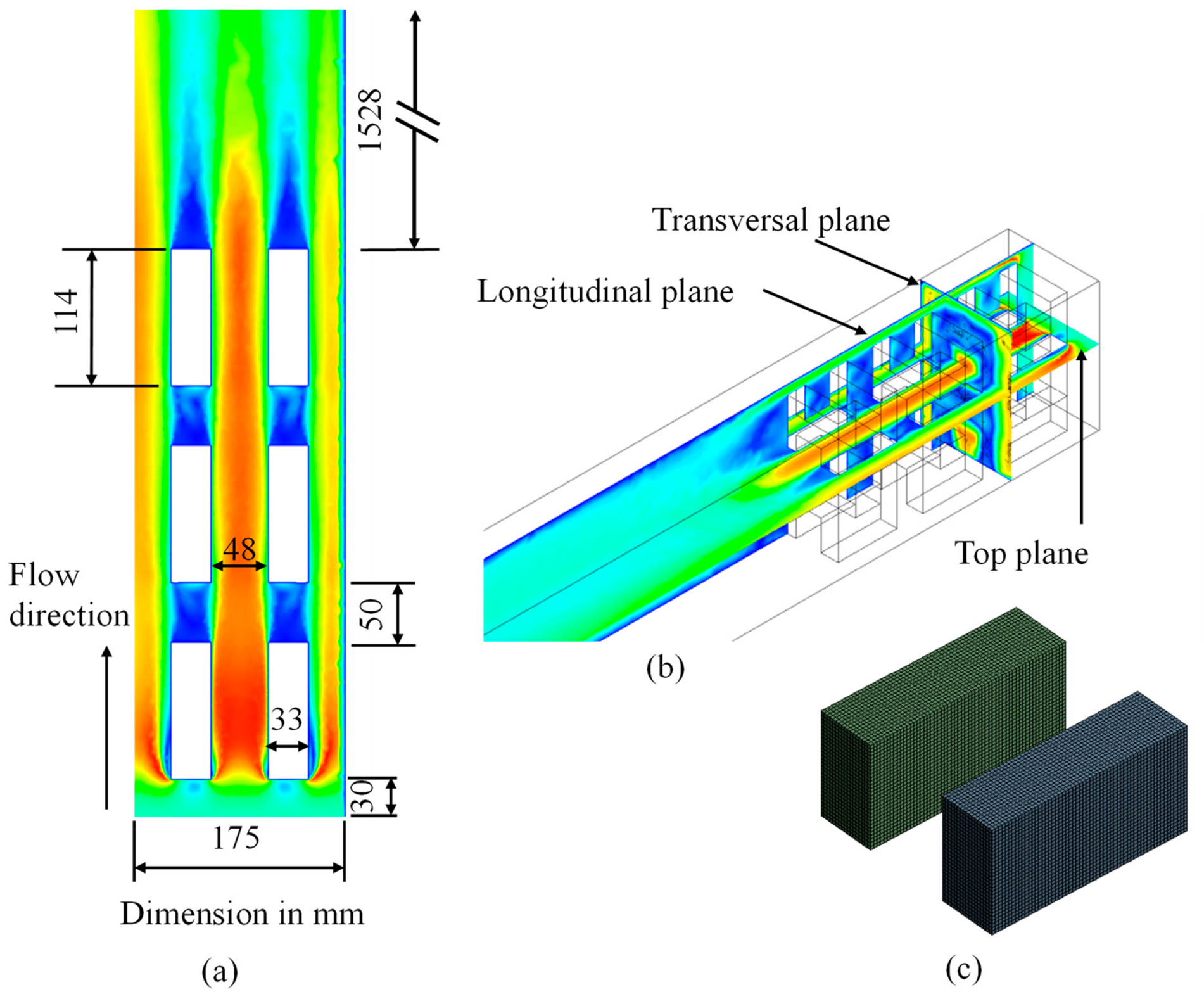
The computational domain contained three brick rows in the streamwise direction. Each row occupied a streamwise length of 114 mm, and the clear spacing between successive rows was 50 mm. The brick setting therefore occupied 3(114) + 2(50) = 442 mm in the streamwise direction. The clear spacing between the two brick columns was 62 mm. The brick dimensions, row and column spacings, wall clearance, and overall arrangement were identical in Settings 1–3; only the vertical-layer locations of the four thermally active brick models differed. Apparent spacing differences in the schematic views result from perspective and source highlighting rather than changes in geometry.
In the experimental facility, a honeycomb flow straightener was installed upstream of the test section to reduce large-scale flow disturbances and establish an approximately uniform velocity distribution before the airflow reached the brick setting. In the CFD model, this conditioned flow was represented directly by imposing a uniform velocity profile at the inlet. A long numerical entrance section was therefore unnecessary, and the inlet boundary was positioned 30 mm upstream of the leading face of the first brick row.
The distance from the trailing face of the third brick row to the pressure-outlet boundary was 1528 mm, completing the total domain length of 2000 mm. This extended downstream region allowed the wakes generated by the brick setting to develop and the airflow to redistribute before reaching the outlet. It also reduced the possibility of outlet-boundary backflow and prevented the pressure-outlet condition from influencing the pressure and velocity fields in and immediately downstream of the brick setting. Thus, the portion of the domain not occupied by bricks represented a downstream flow-development and pressure-recovery region rather than unused computational space.
The study was restricted to the steady convective behavior reproduced by the experimental facility. It does not represent combustion, the firing zone, movement of bricks through an industrial kiln, or the complete transient cooling history of industrial products. Instead, the model examines how the vertical position of a controlled thermal load affects airflow development, surface cooling, and temperature distribution within the brick setting. The term “cooling-zone model” therefore refers to the scaled airflow passage and brick arrangement reproduced from the experimental facility and characterizes the forced-convection environment to which thermally loaded bricks are exposed.
The numerical cases were conducted at free-stream inlet velocities ranging from 2.11 to 3.99 m/s. After accounting for the void fraction of the brick setting, these conditions corresponded to a numerical Reynolds-number range of 16,829–30,641. The published experimental dataset used for validation covered Re = 15,938–30,890 [24]. These ranges are reported separately because the experimental Reynolds numbers were calculated from the measured flow conditions, whereas the numerical values were obtained from the prescribed CFD inlet conditions.
The steady-state Nusselt numbers obtained here can provide convective heat-transfer coefficients for a subsequent transient brick-cooling model through . If the lumped-capacitance criterion is satisfied, a characteristic cooling time may be estimated as . Otherwise, transient conduction within the brick must be resolved. Such an analysis would also require the temperature-dependent brick properties, the initial temperature field, radiative exchange, kiln-wall conditions, and the brick residence time. Consequently, the present steady-state results characterize the relative convective performance of the investigated arrangements but cannot be used directly to predict industrial brick-cooling curves or final outlet temperatures.
2.2. Computational Domains and Investigated Arrangements
Two computational domains were used, as shown in Figure 1. The first reproduced the full width of the experimental test section and was used exclusively for numerical-model validation. This full-domain configuration reproduced Setting 2 of the experimental investigation by Ibrahim et al. [24]. The experimental setting numbers were retained throughout the present CFD study to ensure direct correspondence between the experimental and numerical configurations and eliminate ambiguity in their comparison.
Figure 1.
Computational domains and investigated thermal-source arrangements: (a) full-domain model reproducing experimental Setting 2 reported by Ibrahim et al. [24] and used for numerical validation; and (b) symmetry-reduced domains representing experimental Settings 1–3 and used to compare the three vertical thermal-source arrangements.
Following validation, a symmetry-reduced domain representing one-half of the test section was used for the parametric comparison. The symmetry plane coincided with the longitudinal mid-plane of the geometrically symmetric brick arrangement. This reduced domain reduced the computational cost while retaining the brick passages, wall clearance, thermal-source locations, and relevant flow features required for comparing the vertical arrangements. A symmetry boundary condition was applied at the central longitudinal plane. The symmetry-reduced model was used to predict steady, time-averaged fields under geometrically and hydraulically symmetric boundary conditions. It does not resolve instantaneous asymmetric wake oscillations or vortex shedding, which would require a full-domain transient simulation. The full-domain model was retained for validation against the experimental average Nusselt numbers, while the half-domain model was applied consistently to all three settings for comparative analysis. Accordingly, the reported recirculation patterns represent steady RANS mean-flow structures rather than instantaneous vortical behavior.
Four complete brick-shaped thermal-source models, denoted H1–H4, were included in each configuration. The complete brick lattice, including the number of bricks, their orientations, and the row and column spacings, remained unchanged across the three settings. However, the four thermally active brick models were installed at different vertical-layer positions. Thus, the three settings represent distinct physical heater arrangements reproduced separately in the CFD simulations; they do not represent sequential post-processing of different brick groups within a single unchanged thermal configuration.
In Setting 1, the longitudinal thermal-source models H1 and H2 were located in the third layer, whereas the transverse models H3 and H4 were located in the second layer. In Setting 2, H1 and H2 were located in the first layer, while H3 and H4 remained in the second layer. In Setting 3, H1 and H2 were located in the third layer, whereas H3 and H4 were located in the fourth layer. The horizontal positions and orientations of H1–H4 remained unchanged; only their vertical-layer locations differed among the settings.
The comparison therefore isolates the influence of vertical thermal-source placement while maintaining the same number of bricks, column spacing, row spacing, and total imposed thermal input. The inlet velocity and temperature were not imposed identically across the three settings; instead, each arrangement retained the corresponding measured conditions from the published experiments. Consequently, the actual Reynolds number was used for each numerical case, and the small differences in operating conditions were considered when interpreting the effects of thermal-source placement. Table 1 summarizes the locations of the four thermal sources in the three numerical settings.
Table 1.
Vertical-layer locations and monitored surfaces of the four thermally active brick models.
The monitored surfaces of H1 were denoted LW and LM1, while those of H2 were denoted LC and LM2. LW identifies the longitudinal surface located near the kiln wall, whereas LC identifies the longitudinal surface located near the central passage. LM1 and LM2 identify the corresponding longitudinal surfaces facing the passage between the two brick columns. The monitored surfaces of the transverse models H3 and H4 were denoted T1 and TM1, and T2 and TM2, respectively. All eight surface locations are identified directly in Figure 1.
Figure 2.
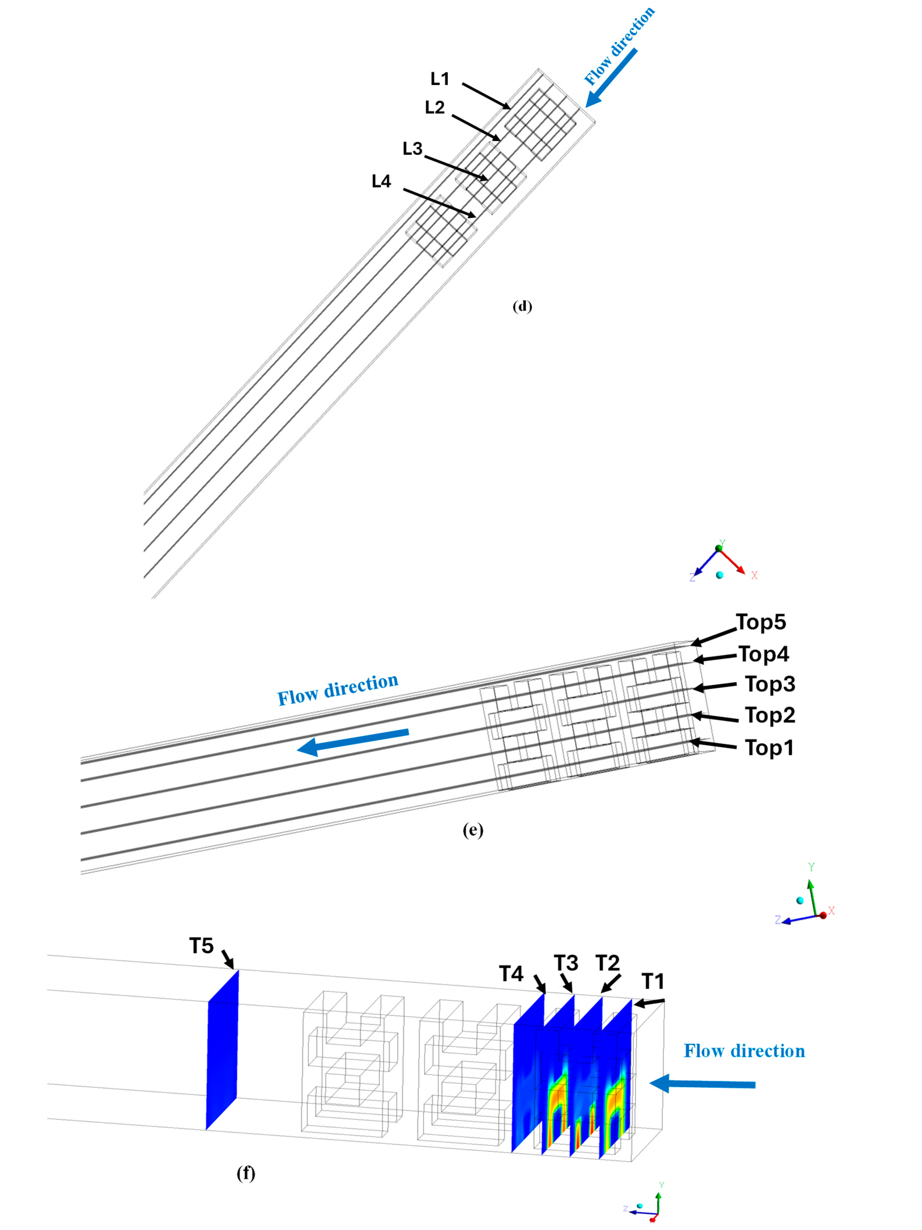
Geometry and discretization of the symmetry-reduced CFD domain: (a) top view of the brick arrangement and flow passages; (b) three-dimensional brick arrangement; (c) representative hexahedral mesh on the solid brick domains; (d) locations of longitudinal planes L1–L4; (e) locations of horizontal planes Top1–Top5; and (f) locations of the transverse temperature-sampling planes T1–T5, with temperature contours displayed only to improve plane visibility and not for quantitative interpretation.
2.3. Representation of the Thermal Sources
All bricks in the experimental setting were represented explicitly as solid refractory-brick domains in the CFD model. Four brick-shaped models, denoted H1–H4, contained electrical heating elements in the experimental facility and therefore acted as the controlled thermal sources [24]. Each heated model had the same external dimensions as the surrounding refractory bricks: 114 mm in length, 33 mm in width, and 58 mm in height. Consequently, changing the locations of the heated models did not alter the overall brick geometry, airflow passages, row spacing, or column spacing. In the numerical model, these four thermally active brick models were represented as solid zones with a uniform volumetric heat-generation rate of . This value was calculated from the electrical power supplied during the experiments and the heated solid volume. The same volumetric heat-generation rate was applied to H1–H4 in all three settings. The steady volumetric heat-generation approach reproduces the controlled laboratory conditions used for validation but does not represent the transient release of stored sensible heat from fired industrial bricks. Consequently, the reported Nusselt numbers and heat-transfer coefficients characterize the convective cooling environment under the investigated conditions, but they cannot be used directly to predict brick-cooling time or final product temperature. Such predictions would require a transient conjugate model incorporating the initial brick-temperature distribution, temperature-dependent material properties, radiation, and kiln-product movement.
The remaining refractory bricks were also included explicitly as solid computational zones but contained no internal thermal source; hence, was assigned to these bricks. Their temperature fields were not prescribed. Instead, they were calculated from heat conduction within the solid domains and conjugate heat exchange with the surrounding airflow. Temperature and normal heat-flux continuity were imposed at every air–brick interface.
The electrical elements served as controlled laboratory thermal surrogates that maintained stable and repeatable thermal conditions for evaluating convective heat transfer. They should not be interpreted as industrial electrical heaters or as a representation of continuous heat generation within bricks passing through an actual cooling zone. In an operating tunnel kiln, fired bricks enter the cooling zone at elevated temperatures and release stored sensible heat while their temperatures decrease with time. A transient model based on an initial brick-temperature distribution would therefore be required to predict the actual cooling curves or the final product temperature.
The present steady thermal-source formulation was adopted to reproduce the experimental procedure reported in Reference [24], in which measurements were recorded only after stable inlet, outlet, and brick-surface temperatures had been attained. Under these conditions, the imposed electrical input provides the temperature difference required to determine the local and average convective heat-transfer characteristics. Accordingly, the results should be interpreted as steady forced-convection performance indicators for the scaled cooling-zone arrangement rather than as direct predictions of the transient thermal history of industrial bricks. The locations of H1–H4 and their monitored surfaces are identified in Figure 1 and Table 1. The four thermal sources reproduce the controlled heated-brick arrangement used in the experimental facility of Ibrahim et al. [24]. This arrangement was designed to isolate the influence of source position under measurable and repeatable conditions; it does not represent a complete population of simultaneously cooling bricks in an industrial kiln. Accordingly, the three settings are used here to examine the mechanisms by which vertical source placement affects local airflow, convective heat transfer, and ideal pumping-power requirements. The resulting comparisons are restricted to the investigated scaled geometry and should not be interpreted as direct predictions of whole-kiln cooling performance.
2.4. Post-Processing Planes
In addition to the eight monitored brick surfaces defined in Table 1 and identified in Figure 1, a set of geometrical post-processing planes was defined to examine the spatial development of the flow and thermal fields. The monitored-surface abbreviations LW, LM1, LC, LM2, T1, TM1, T2, and TM2 refer to specific surfaces of the thermally active brick models. In contrast, the plane labels L1–L4, T1–T5, and Top1–Top5 refer to geometrical sampling sections within the CFD domain. Although some labels contain similar characters, the monitored brick surfaces and post-processing planes represent different quantities.
The locations of the post-processing planes are shown explicitly in Figure 2d–f and are summarized in Table 2. The longitudinal planes L1–L4 were used to evaluate near-wall flow, thermal-source–channel interactions, and airflow development between adjacent columns. The transverse planes T1–T5 followed the flow from the first heated row to the region downstream of the brick setting. The horizontal planes Top1–Top5 passed through the four brick layers and the near-roof region, allowing vertical variations in velocity and temperature to be identified.
Table 2.
Locations and purposes of the longitudinal, transverse, and horizontal monitoring planes used for CFD post-processing.
These planes were used consistently for all three arrangements, so their physical sampling locations did not change. Because the inlet velocity and temperature were setting-specific, comparisons were made using the corresponding Reynolds number of each case. This approach removes the post-processing location as a source of variation while retaining the actual experimental operating conditions when interpreting the effects of thermal-source placement.
2.5. Governing Equations and Turbulence Model
The airflow was treated as three-dimensional, steady, incompressible, and turbulent. The numerical model solved the Reynolds-averaged conservation equations for mass, momentum, and energy. Heat conduction was solved simultaneously within the heated and unheated brick domains. Gravity and density-dependent buoyancy terms were not included; therefore, the model represents forced-convection cooling. The governing equations presented below are the steady Reynolds-averaged conservation equations for mass, momentum, and energy, together with solid heat conduction and conjugate interface conditions. These equations follow the standard transport equation formulation and were not derived or calibrated from the present experimental measurements. The turbulence-closure equations, blending functions, and associated coefficients correspond to the baseline BSL – formulation proposed by Menter [29].
The continuity equation is expressed as:
The momentum equation is:
The Reynolds stresses were related to the mean velocity gradients using the Boussinesq eddy-viscosity hypothesis:
where ui is the mean velocity component, p is the static pressure, ρ and μ are the air density and dynamic viscosity, respectively, k is the turbulent kinetic energy, μt is the turbulent dynamic viscosity, and δij is the Kronecker delta.
The steady energy equation in the fluid domain is:
where Tf, cp, kf, and Prt denote the air temperature, specific heat, thermal conductivity, and turbulent Prandtl number, respectively.
Heat conduction within the solid brick domains was calculated from:
where Ts and ks are the solid temperature and thermal conductivity, respectively. A uniform volumetric heat-generation rate of 3.377413 × 10⁶ W m−3 was imposed within the heated brick models. For the surrounding unheated bricks, q‴ was set to zero.
Conjugate heat transfer between the airflow and the brick surfaces was imposed through the continuity of temperature and normal heat flux:
where the effective thermal conductivity of the fluid is defined as:
The baseline BSL – model was used to close the Reynolds-averaged momentum equations. The model employs the – formulation in the near-wall region and gradually transforms into a –-type formulation in the outer flow region through the blending function . This approach retains the near-wall performance of the – model while reducing its sensitivity to free-stream values. The transport equations, blending functions, and model constants presented below follow the standard BSL formulation reported by Menter [29].
The turbulent kinetic-energy equation is:
The specific-dissipation-rate equation is:
where the cross-diffusion contribution is:
The production of turbulent kinetic energy is defined as:
The turbulent viscosity is evaluated from:
The coefficients of the BSL model are calculated by blending the inner and outer coefficient sets:
where φ represents γ, β, σk, or σω. The blending function F1 approaches unity near solid surfaces, where the k–ω formulation is applied, and approaches zero in the outer flow region, where the transformed k–ε formulation is used. It is defined as:
where:
and:
Here, y is the distance from the nearest solid surface. The model constants were β* = 0.09, σk1 = 0.50, σω1 = 0.50, β1 = 0.075, γ1 = 5/9, σk2 = 1.00, σω2 = 0.856, β2 = 0.0828, and γ2 = 0.44. The model coefficients are the standard constants associated with the selected BSL – formulation [29]. They were taken from the published turbulence-model formulation and were not determined from, or adjusted using, the experimental measurements employed for validation. The same coefficients were retained for all numerical cases.
Only forced convection in the air and heat conduction within the solid domains were considered. Thermal radiation was not included. Therefore, the conclusions are restricted to the temperature range and operating conditions represented by the scaled cooling-zone experiment.
The simulations considered forced convection and neglected buoyancy and surface-to-surface radiation. The maximum Richardson number, estimated using the brick height (L = 0.058 m), the minimum inlet velocity (2.111 m/s), and the maximum fluid-temperature difference of approximately 30 K, was about 0.013. Because , buoyancy was considered small relative to the imposed airflow. Radiation was assessed conservatively using blackbody exchange between the maximum plotted temperature of 51.5 °C and an ambient temperature of 22 °C, giving an upper-bound net radiative heat flux of approximately 200 W/m2. In comparison, the imposed volumetric heat generation corresponds to approximately 737 W per active brick, or an average generated heat flux of about 30 kW/m2 over its external surface. The blackbody upper bound is therefore below 0.7% of the generated heat flux, while the actual contribution would be smaller because the surface emissivity is below unity and the surrounding surfaces are warmer than the inlet air. These estimates support neglecting buoyancy and radiation for the present low-temperature, forced-convection experiment, but not for an industrial kiln operating at substantially higher temperatures.
2.6. Boundary Conditions
The numerical boundary conditions were defined to reproduce the steady operating conditions of the 1:4-scale experimental facility. A uniform velocity profile was imposed at the inlet plane, located 30 mm upstream of the leading face of the first brick row. The experimental facility employed a honeycomb flow straightener to establish an approximately uniform approach flow; this conditioned flow was represented directly by the uniform CFD inlet condition.
Six operating points were simulated for each thermal-source arrangement. The prescribed inlet velocities were 2.111, 3.070, 3.376, 3.517, 3.892, and 3.990 m/s for Settings 1 and 3 and 2.180, 3.010, 3.517, 3.780, 3.903, and 3.968 m/s for Setting 2. The inlet-air temperature was specified separately for each case using the corresponding measured experimental value. The setting-specific inlet velocities and inlet-air temperatures prescribed in the CFD simulations are summarized in Table 3. The inlet turbulence intensity was 5%, and the hydraulic diameter of the brick setting was 0.0852 m.
Table 3.
Setting-specific inlet velocity and inlet air temperature boundary conditions used in the CFD simulations.
A pressure-outlet condition at zero gauge pressure was imposed at the domain exit, located 1528 mm downstream of the trailing face of the final brick row. This downstream length allowed the wakes generated by the brick setting to develop and reduced the possibility of outlet-boundary backflow affecting the pressure and velocity fields near the bricks. All brick and duct surfaces were treated as stationary no-slip walls. The external duct walls were considered adiabatic, consistent with the insulated experimental test section.
At every air–brick interface, coupled thermal conditions were applied to enforce continuity of temperature and normal heat flux. A uniform volumetric heat-generation rate of 3.377413 × 10⁶ W m−3 was imposed within each of the four thermally active brick models H1–H4. The remaining refractory bricks were assigned no internal heat generation, , and their temperatures were calculated from solid conduction and conjugate heat exchange with the airflow. The adiabatic-wall condition represents an idealization of the experimental test section. A quantitative external heat-loss boundary condition could not be prescribed because the published experiment [24] does not provide the wall thermal conductivity, insulation thickness, external surface temperature, or ambient heat-transfer coefficient required to determine the wall heat flux. Introducing an estimated correction would therefore add an unconstrained parameter to the validation. The walls were consequently treated as adiabatic, and the effect of this assumption is reflected in the numerical–experimental deviation reported in Section 3.1, particularly at the three highest Reynolds numbers.
For the symmetry-reduced simulations, a symmetry condition was imposed at the central longitudinal plane. This condition specified zero velocity normal to the symmetry plane and zero normal gradients of all transported variables. Gravity was not activated, and density-dependent buoyancy was therefore excluded. Thermal radiation was also omitted. Consequently, the numerical results represent steady forced-convection heat transfer within the temperature and Reynolds-number ranges of the scaled experimental facility.
2.7. Material Properties
In the experimental work of Ibrahim et al. [24], fixed air properties were used in the data-reduction calculations. The published experimental Reynolds and Nusselt numbers were retained directly for the validation comparison. In the CFD simulations, however, the air density, dynamic viscosity, specific heat capacity, and thermal conductivity were evaluated at the inlet-air temperature corresponding to each operating condition. The air properties, therefore, varied among the numerical cases and were not represented by a single set of values in Table 4. The heated and unheated bricks were modeled as homogeneous and isotropic solid domains with identical thermophysical properties. The volumetric heat-generation term was applied only to the heated bricks. The brick properties used in the CFD simulations are listed in Table 4.
Table 4.
Thermophysical properties of the refractory bricks used in the CFD simulations.
The air properties corresponded to the representative temperature of the experimental tests, whereas the refractory-brick properties represented the material used in the validation facility. The same property definitions were applied to the full-domain validation model and the three half-domain heater configurations.
2.8. Mesh-Independence and Mesh-Quality Assessment
A mesh-independence assessment was conducted before performing the final simulations. The fluid and solid domains were discretized predominantly using structured hexahedral elements. Local refinement was applied near brick surfaces and edges, within narrow airflow passages, and in downstream wake regions, where comparatively large velocity and temperature gradients were expected. A representative view of the computational mesh is presented in Figure 2c.
The full-domain validation configuration at an inlet velocity of 2.11 m/s, corresponding to Re = 16,829, was used to assess the mesh. Five progressively refined meshes were examined, and the area-averaged Nusselt number was selected as the mesh-sensitivity parameter because it represents the overall convective heat-transfer response of the thermally active brick models. Mesh independence was considered achieved when the difference between two successive meshes was less than 1%, using the finer-mesh result as the reference.
As shown in Table 5, refining the mesh from 2,846,008 to 4,491,230 elements changed the average Nusselt number from 160.67 to 161.28, corresponding to a difference of 0.38%. This value was the resulting variation rather than a more restrictive predefined criterion. The 4,491,230-element mesh was the first mesh in the tested sequence to satisfy the adopted 1% requirement and was therefore selected for the final full-domain validation simulations. Thus, applying a 1% criterion would still select the same mesh, and no alternative mesh or computational time corresponding to an exact 1% variation exists within the tested sequence.
Table 5.
Results of the mesh-independence assessment.
The maximum skewness of the selected mesh was 0.92, remaining below the commonly accepted upper limit of 0.95 for complex CFD meshes. The numerical convergence was also assessed using the residual histories and the stability of the monitored average Nusselt number and heated-surface temperature. The same element-size controls and local-refinement strategy were subsequently applied to the symmetry-reduced configurations.
2.9. Numerical Convergence Criteria
The steady numerical solution was considered converged when the scaled residuals decreased below 10−4 for the continuity and momentum equations, and below 10−6 for the energy equation. The stricter energy-equation criterion was adopted because the principal outputs of the study, surface temperature, local and average Nusselt numbers, and temperature non-uniformity, depend directly on the accuracy and stability of the conjugate heat-transfer solution. Residual reduction was not used as the sole convergence indicator. The area-averaged Nusselt number and the mean temperature of the thermally active brick surfaces were monitored throughout the iterative solution. Iterations continued until the prescribed residual limits were satisfied and both monitored quantities became stable, with no systematic change during subsequent iterations. The same convergence requirements were applied to the full-domain validation cases and all symmetry-reduced thermal-source configurations.
A separate parametric assessment with less restrictive residual limits was not performed because the adopted criteria yielded stable thermal quantities across all cases and were applied consistently throughout the study. Although less restrictive limits could reduce the number of iterations, terminating the solutions earlier was not considered appropriate without confirming the stability of the heat-transfer quantities central to the present analysis.
2.10. Calculation of the Reynolds and Nusselt Numbers
To maintain consistency with the experimental validation data of Ibrahim et al. [24], the Reynolds number, local convective heat-transfer coefficient, and local Nusselt number were evaluated using the definitions adopted in the experiments. The Reynolds number was calculated from the interstitial air velocity as:
where is the interstitial air velocity, is the hydraulic diameter of the brick setting (0.0852 m), and is the kinematic viscosity of air. The interstitial velocity was calculated from the prescribed superficial inlet velocity, , using
where is the geometric void fraction of the brick setting. This was calculated as the ratio of the open flow area to the total duct cross-sectional area:
Thus, the value 0.756 represents the proportion of the duct cross-section available for airflow and is not a surface-emissivity value. Thermal radiation was not included in the numerical model; therefore, no surface emissivity was specified. For the validation cases, the Reynolds numbers reported in the published experimental dataset were retained. For the numerical parametric cases, the Reynolds number was calculated using the same definitions as in the experiment, with the air kinematic viscosity evaluated at the corresponding inlet air temperature.
The local convective heat-transfer coefficient at the ith monitored heated-brick surface was calculated as:
where is the heat input to the th heated brick, is its wetted surface area , is the mean temperature of the monitored heated-brick surface, and is the inlet-air temperature. For the experimental validation data, , where and are the measured voltage and current, respectively. In the CFD model, the corresponding heat input was obtained from the prescribed volumetric heat-generation rate as .
The corresponding local Nusselt number was calculated from the following equation:
where is the thermal conductivity of air. The average Nusselt number for each configuration was calculated from the area-weighted mean of the local Nusselt numbers over the monitored heated-brick surfaces:
where and are the local Nusselt number and area of the -th monitored surface, respectively, and is the total number of monitored surfaces. Because all monitored surfaces had equal areas, the area-weighted expression was reduced to the arithmetic mean:
The same averaging procedure and property definitions were applied to the numerical predictions and experimental measurements used for validation.
3. Results and Discussion
3.1. CFD Model Validation
The CFD model was validated against the experimental measurements reported by Ibrahim et al. [24]. The full computational domain was used for this validation to reproduce the experimental test section without applying the symmetry assumption. The comparison covered Reynolds numbers from approximately 16,000 to 31,000 and included both local and average Nusselt numbers.
Figure 3 compares the experimental and numerical local Nusselt numbers at the four heated-brick locations. For consistency with the notation of Ibrahim et al. [24], the experimental locations are denoted LW, LM, T, and TM, while the corresponding CFD monitoring locations plotted in Figure 3 are denoted LW, LC, T1, and T2, respectively. The CFD results reproduced the experimentally observed increase in the local Nusselt number with Reynolds number at all four positions. This increase results from the higher airflow velocity through the brick passages, which reduces the thermal boundary-layer thickness and enhances convective heat transfer from the heated surfaces.
Figure 3.
Comparison of the predicted and experimental local Nusselt numbers at the heated-brick locations: (a) transverse positions T and TM and (b) longitudinal positions LW and LM. Experimental data adapted from Ibrahim et al. [24] under the CC BY license.
The numerical model also reproduces the differences between the longitudinal and transverse heater positions. Longitudinal heaters generally exhibit higher local Nusselt numbers because both major surfaces are exposed to the airflow passing through the longitudinal channels. In contrast, flow separation and wake formation downstream of the transverse heaters reduce the local airflow velocity over portions of their surfaces, thereby decreasing the local heat-transfer rate. The agreement in these position-dependent trends indicates that the model captures the principal effects of heater orientation and surrounding flow structure.
Figure 4 compares the experimentally measured and numerically predicted average Nusselt numbers. Both datasets showed a continuous increase in the average Nusselt number with Reynolds number. For the first three operating conditions, the signed deviations between the CFD predictions and experimental measurements were 2.41%, −0.36%, and 2.90%, respectively. At the three higher Reynolds numbers, the deviations increased to 8.90%, 11.68%, and 13.02%, respectively. The absolute deviations, therefore, ranged from 0.36% to 13.02%, with a mean absolute deviation of approximately 6.55%. The mean value is reported only as an overall summary and should be interpreted together with the individual deviations, particularly those at the three highest Reynolds numbers.
Figure 4.
Comparison of the predicted and experimental average Nusselt numbers over the investigated Reynolds-number range. Experimental data adapted from Ibrahim et al. [24] under the CC BY license.
The experimental uncertainty analysis reported by Ibrahim et al. [24] was based on the Kline–McClintock root-sum-square method. The reported average uncertainties were ±2.5% for superficial velocity, ±2.7% for interstitial velocity, ±3.1% for Reynolds number, ±0.69% for the average heat-transfer coefficient, ±3.3% for pressure drop, ±4.5% for friction factor, ±1.6% for the average Nusselt number, and ±2.12% for heat input. The first three CFD predictions were close to the experimental measurements, whereas the deviations of 8.90%, 11.68%, and 13.02% at the higher Reynolds numbers exceeded the experimental Nusselt-number uncertainty. Consequently, the validation should not be interpreted as agreement within experimental uncertainty across the complete operating range.
The increasing deviation at higher Reynolds numbers may reflect the greater sensitivity of separated passage flow and interacting wakes to turbulence-model assumptions, near-wall treatment, surface roughness, and small geometric imperfections. Additional differences may arise because the numerical model assumes smooth surfaces and adiabatic external walls, whereas the experimental facility may experience surface roughness, leakage, and residual heat loss. These factors are offered as possible contributors rather than as a quantitative correction for the observed discrepancies. The increase in deviation from 8.90% to 13.02% at the three highest Reynolds numbers indicates reduced quantitative accuracy of the adopted numerical formulation under conditions where flow separation and wake interactions become stronger. Accordingly, the model is not claimed to provide uniformly accurate absolute predictions over the complete Reynolds-number range. The higher-Reynolds-number results are used primarily to compare the three arrangements and interpret their flow and heat-transfer mechanisms under a consistent numerical framework. A systematic comparison with alternative turbulence closures, such as the SST – or low-Reynolds-number models, remains necessary before extending the model’s absolute predictive capability.
No arbitrary acceptance threshold was imposed. The validation demonstrates that the model reproduces the measured trend and the relative dependence of the Nusselt number on Reynolds number, with stronger quantitative agreement at the lower and intermediate operating points and reduced accuracy at the three highest points. The subsequent CFD results are therefore used primarily for comparative and mechanistic assessment of the three thermal-source arrangements within the investigated geometry and Reynolds-number range. Absolute predictions at the upper end of the range should be interpreted in light of the reported maximum deviation of 13.02%.
3.2. Flow Field Characteristics
All three settings contained the same number, dimensions, and spatial arrangement of solid bricks; only the locations of the imposed volumetric heat generation differed. Under the adopted forced-convection formulation, thermal-source relocation does not alter the flow geometry or introduce an additional momentum source. Consequently, the principal airflow passages and mean recirculation regions are expected to remain closely comparable at similar inlet conditions. The velocity contours and streamlines are used to illustrate this behavior, while the pressure-drop results in Section 3.7 provide an integral quantitative measure of the aerodynamic response. The discussion therefore refers to comparable principal flow topology rather than claiming identical local velocity fields.
For the following discussion, an operating point denotes one setting-specific combination of prescribed inlet velocity and inlet-air temperature. Six operating points were simulated for each thermal-source arrangement, as reported in Table 3. Because the experimental inlet conditions were retained, the velocities and temperatures at a given operating-point number were not necessarily identical among the three settings. The following analyses are based on the half-domain model with a longitudinal symmetry plane. Velocity contours, streamlines, and velocity vectors were examined at the monitoring planes defined in Table 2 to clarify the airflow behavior within and around the brick arrangement.
3.2.1. Velocity Contours
Figure 5 presents velocity-magnitude contours at longitudinal plane L3. As shown in Figure 2d and defined in Table 2, L3 is a vertical streamwise plane located within the central airflow passage between the two longitudinal brick columns. It extends from the inlet to the outlet of the 2000 mm computational domain and captures airflow acceleration through the restricted brick passages, wake formation downstream of the bricks, and subsequent momentum recovery. The inlet boundary was located 30 mm upstream of the leading face of the first brick row. The three-row brick setting occupied 442 mm in the streamwise direction, while the remaining 1528 mm formed the downstream flow-development and pressure-recovery region. These dimensions were identical for all three configurations.
Figure 5.
Velocity-magnitude contours at longitudinal plane L3: (a) effect of inlet velocity for Setting 2 at U1 = 2.180 m/s, U3 = 3.517 m/s, and U6 = 3.968 m/s; and (b) comparison at the lowest setting-specific inlet velocities of 2.180 m/s for Setting 2 and 2.111 m/s for Settings 1 and 3.
- Effect of inlet velocity
Figure 5a compares the velocity distributions for Setting 2 at its first, third, and sixth operating points, corresponding to inlet velocities of U1 = 2.180 m/s, U3 = 3.517 m/s, and U6 = 3.968 m/s. At U1, the incoming airflow remains relatively uniform before reaching the brick arrangement. The reduction in the available flow area between adjacent brick columns causes the air to accelerate within the principal longitudinal passages. Lower-velocity regions form near the brick surfaces and immediately downstream of the brick edges due to boundary-layer development and flow separation. Increasing the inlet velocity to U3 increases the velocity throughout the computational domain without substantially changing the overall flow topology. The high-velocity cores within the central passages become more pronounced and extend further downstream. At the same time, stronger velocity gradients develop near the brick surfaces, indicating increased momentum transfer and a greater potential for convective heat removal.
At U6 = 3.968 m/s, the airflow is strongly concentrated within the open channels between the brick columns. Continuous high-velocity regions extend through most of the brick setting, while low-velocity wakes remain downstream of the transverse brick faces. The stronger channel flow and near-wall velocity gradients explain the increase in the local and average Nusselt numbers with increasing Reynolds number. Nevertheless, the persistence of low-velocity wake regions indicates that increasing the inlet velocity alone does not eliminate local flow non-uniformity within the brick arrangement.
- Effect of heater position
Figure 5b compares the velocity fields at the lowest available operating point for each setting: 2.180 m/s for Setting 2 and 2.111 m/s for Settings 1 and 3. Despite the approximately 3.3% difference in inlet velocity, the three configurations displayed closely comparable velocity distributions, including similar acceleration through the central passages and comparable low-velocity regions near and behind the brick surfaces. This similarity is primarily due to the common brick geometry and outlet conditions. Because gravity and buoyancy were not included, changing the heated-brick elevation does not directly generate a new main-flow structure. Small differences among the contours may reflect both the setting-specific inlet condition and local momentum redistribution; they should not be interpreted as a major heater-induced change in the flow regime. The effect of heater placement is therefore evaluated through the position of each heated surface relative to the established passages and wakes, with the actual Reynolds number of each case retained in the quantitative comparisons.
These results demonstrate that inlet velocity governs the magnitude of the airflow and the strength of convective transport, whereas heater placement determines how effectively the established mean-flow structure interacts with the heated surfaces. The thermal differences among the three configurations should therefore be interpreted primarily in terms of the local velocity around each heated brick, rather than in terms of changes in the overall airflow pattern.
3.2.2. Streamline Analysis
Figure 6 presents the streamline patterns at longitudinal plane L3 for Settings 1–3 at their highest operating points. As shown schematically in Figure 2d, L3 is a vertical streamwise plane located within the central airflow passage between the two longitudinal brick columns. The plane extends along the computational-domain length and intersects the principal flow passage through the brick setting, allowing the acceleration between the bricks, flow separation, wake formation, and downstream momentum recovery to be examined. The corresponding inlet velocities were 3.990 m/s for Settings 1 and 3 and 3.968 m/s for Setting 2. The streamlines are colored according to the local velocity magnitude.
Figure 6.
Streamlines colored by local velocity magnitude at longitudinal plane L3, located in the central airflow passage between the two longitudinal brick columns: (a) Setting 1 at 3.990 m/s; (b) Setting 2 at 3.968 m/s; and (c) Setting 3 at 3.990 m/s. The location and orientation of plane L3 are shown in Figure 2d.
In all three settings, the incoming airflow is diverted around the upstream brick surfaces and accelerates through the restricted passages between adjacent brick columns. The streamlines become closely spaced inside these passages, indicating the formation of high-velocity flow cores. Downstream of the brick edges, the flow separates, producing lower-velocity wake regions. Partial flow reattachment occurs before the air encounters the subsequent brick rows, creating repeated cycles of acceleration, separation, and wake development throughout the setting.
Small recirculation regions are visible behind several transverse brick faces and within locally sheltered parts of the arrangement. These regions are produced by the adverse pressure gradient that develops after the airflow passes the brick edges. Air trapped within the recirculation zones exchanges momentum with the surrounding high-velocity flow through the separated shear layers. This interaction promotes local mixing but produces non-uniform convective conditions over the brick surfaces.
The streamline patterns are closely comparable because the brick geometry was identical and the highest-point inlet velocities differed by less than 0.6%. Under the adopted forced-convection assumptions, source elevation does not create a fundamentally different mean-flow structure. Instead, thermal performance depends on whether each heated surface lies near a high-velocity passage, a separated shear layer, or a low-velocity wake. The streamlines therefore support the interpretation of source exposure without implying identical local velocity fields.
3.2.3. Transverse Flow Structures
Velocity-vector distributions were examined at transverse planes T2 and T4 to clarify the redistribution of airflow across the width and height of the brick arrangement. Plane T2 is located in the gap between heaters H3 and H4, whereas plane T4 is positioned downstream of the first brick row and midway between two adjacent rows. The two planes therefore represent the airflow within the brick region and its subsequent development after passing the first row.
Figure 7a–c presents the velocity vectors at plane T2. The airflow is concentrated within the open passages between the brick columns, producing a high-velocity core in the central region. As the air encounters the brick surfaces, part of the flow is redirected laterally and vertically toward the neighboring passages. Lower-velocity regions occur near brick surfaces, duct walls, and locally sheltered areas. Small counter-rotating circulation structures also develop around certain passages due to the interaction between the accelerated core flow and the surrounding lower-velocity air.
Figure 7.
Velocity-vector distributions at transverse planes T2 (a–c) and T4 (d–f) for Setting 1 (a,d), Setting 2 (b,e), and Setting 3 (c,f) at their highest operating points. The corresponding inlet velocities were 3.990, 3.968, and 3.990 m/s, respectively.
Figure 7d–f shows the flow behavior at plane T4. At this downstream position, the airflow has already interacted with the first brick row. The vector field therefore reflects the combined effects of flow separation, wake development, and momentum recovery. The high-velocity air leaving the restricted passages interacts with the slower air in the downstream wakes, causing the lateral redistribution of momentum across the section. The circulation structures become more clearly developed between adjacent passages, while low-velocity regions remain behind the transverse brick faces.
The vector distributions are closely comparable for Settings 1–3 because the brick geometry was unchanged and the highest-point inlet velocities were nearly matched. Changing the vertical position of the heated bricks does not significantly modify the cross-sectional momentum distribution under the forced-convection assumptions used in the model. Any residual differences may include the small effect of the setting-specific inlet velocity and temperature. Accordingly, the transverse-flow results should not be interpreted as evidence that one heater setting produces a fundamentally stronger circulation pattern than another.
The vector plots identify where the established airflow can provide effective convective cooling. Surfaces adjacent to accelerated passages experience stronger momentum transport, whereas wall-adjacent and wake-sheltered surfaces experience weaker convection. Together with the longitudinal contours and streamlines, these results show that the brick arrangement governs the principal mean-flow topology while source placement determines the exposure of the heated surfaces to high-velocity cores, shear layers, and wakes.
3.3. Temperature Distribution Characteristics
The temperature field was examined at longitudinal, transverse, and horizontal monitoring planes to determine how the inlet condition and heater location affect heat removal and thermal spreading within the brick arrangement. The airflow fields remained closely comparable at corresponding operating points because the geometry was unchanged, whereas the temperature distribution responded directly to the location of the volumetric heat source. The setting-specific inlet velocities and temperatures were retained when interpreting these thermal differences.
3.3.1. Longitudinal Temperature Distribution
Figure 8 presents the air-temperature contours at longitudinal plane L3 for Settings 1–3 under their lowest and highest operating conditions. As shown in Figure 2d, L3 is a vertical plane located at the fixed lateral coordinate mm within the central airflow passage between the two longitudinal brick columns. The -axis denotes the streamwise direction, the -axis the vertical direction, and the -axis the lateral direction across the duct width. The plane extends from the inlet to the outlet and over the complete 250 mm domain height. Accordingly, Figure 8 presents longitudinal side views rather than transverse cross-sections.
Figure 8.
Air-temperature contours at longitudinal plane L3, a vertical (y)-(z) plane located at (x = 15.5) mm within the central airflow passage between the two longitudinal brick columns: (a) Setting 1 at 2.111 m/s; (b) Setting 2 at 2.180 m/s; (c) Setting 3 at 2.111 m/s; (d) Setting 1 at 3.990 m/s; (e) Setting 2 at 3.968 m/s; and (f) Setting 3 at 3.990 m/s. The airflow proceeds from left to right in the positive (z)-direction. The contours show the fluid-temperature field; the solid brick regions are masked and appear white. The location of L3 is shown in Figure 2d.
The lowest-point inlet velocities were 2.111 m/s for Settings 1 and 3 and 2.180 m/s for Setting 2. At the highest operating points, the corresponding velocities were 3.990, 3.968, and 3.990 m/s for Settings 1, 2, and 3, respectively. A common temperature scale of 22.0–51.5 °C was used for all six contours, enabling direct visual comparison under comparable, although not identical, inlet conditions.
The contours represent the fluid-temperature field at plane L3. The solid brick regions are excluded from the displayed fluid contours and consequently appear white. Therefore, the red and yellow regions indicate relatively high air temperatures adjacent to the thermally active brick models rather than prescribed brick temperatures. Because the simulations were steady, no initial brick temperatures were imposed. The four thermally active brick models H1–H4 contained the prescribed volumetric heat-generation term, whereas the remaining refractory bricks were assigned . The temperatures of all solid brick domains were calculated through heat conduction and conjugate heat exchange with the airflow.
At the lowest operating points, broad warm-air regions develop near the thermally active bricks in all three settings. The lower airflow velocity provides weaker convective heat removal and a longer residence time within the brick passages. Consequently, the thermal influence of the heated models extends farther into the surrounding airflow, and steep temperature gradients form between the heated regions and the cooler incoming air. The vertical and streamwise locations of these warm regions vary across settings because the thermally active brick models occupy different vertical layers.
At the highest operating points, the increased airflow velocity reduces the extent and intensity of warm-air regions. Stronger forced convection removes heat more effectively from the thermally active surfaces, while a higher mass flow rate limits the air’s temperature rise. Consequently, the red and yellow regions observed at the lower operating points become smaller or shift toward lower temperature levels. This behavior is consistent with the increase in Nusselt number with Reynolds number. The three settings retained closely comparable velocity fields at corresponding operating points because their brick geometry was identical. Their temperature fields nevertheless differed because the thermally active surfaces occupy different positions relative to the established high-velocity passages, separated-flow regions, and wakes. Surfaces exposed to faster passage flow transfer heat more effectively and generate less extensive high-temperature regions, whereas surfaces located near sheltered or low-velocity regions produce more concentrated warm zones. The small setting-specific differences in inlet velocity and inlet temperature may also contribute to the observed thermal differences.
In Setting 2, where the longitudinal thermal sources occupy the first layer, the warm region is concentrated mainly in the lower portion of the longitudinal plane. Setting 1 shifts the longitudinal sources to the third layer, moving a greater part of the heated region upward. Setting 3 places the longitudinal sources in the third layer and the transverse sources in the fourth layer, producing the strongest upper-level thermal influence and a localized high-temperature region near the downstream thermally active model. In all three settings, increasing the airflow velocity reduced the extent of these warm regions.
The contours demonstrate that inlet velocity governs the overall intensity and spread of the temperature field, while thermal-source placement determines the locations of the principal warm zones. However, contour plots alone cannot establish the most favorable configuration. The quantitative comparisons of local and average Nusselt numbers and heated-surface temperature non-uniformity are therefore presented in the following sections.
3.3.2. Cross-Sectional Temperature Distribution
Figure 9 compares the air-temperature distributions at transverse planes T2 and T4 for the three settings at their highest operating points. The inlet velocity was 3.968 m/s for Setting 2 and 3.990 m/s for Settings 1 and 3. Plane T2 is located between thermal-source models H3 and H4, whereas T4 is positioned downstream of the first brick row, midway between two adjacent rows. A common temperature scale was used for all six contours, enabling a comparison of the location and extent of the heated regions under nearly matched flow conditions.
Figure 9.
Cross-sectional air-temperature contours at the highest setting-specific operating points. Panels (a–c) show transverse plane T2, located between thermally active brick models H3 and H4: (a) Setting 1 at 3.990 m/s; (b) Setting 2 at 3.968 m/s; and (c) Setting 3 at 3.990 m/s. Panels (d–f) show transverse plane T4, located downstream of the first brick row and midway between two successive rows: (d) Setting 1 at 3.990 m/s; (e) Setting 2 at 3.968 m/s; and (f) Setting 3 at 3.990 m/s. A common temperature scale was used for all panels. The contours show the fluid-temperature field, while the solid brick regions are masked. The locations of planes T2 and T4 are shown in Figure 2f.
At plane T2, the highest air temperatures occurred near the thermally active brick surfaces. In Setting 2, the warm region was concentrated mainly in the lower part of the cross-section, while the upper portion remained comparatively cool. Setting 1 produced a centrally located heated region that extended above and below the source level, whereas Setting 3 shifted the warm region toward the upper part of the brick setting. These distributions reflect the different vertical locations of the thermal sources.
Lower-temperature regions occurred within the open airflow passages and near the duct boundaries, where the air had less thermal contact with the heated surfaces. The largest temperature gradients developed immediately adjacent to the thermally active bricks. The heated air subsequently spread into the neighboring passages through forced convection and mixing.
At plane T4, the localized high-temperature regions observed at T2 became weaker and more diffuse. This behavior results from downstream heat transport and mixing with the cooler core airflow after passage through the first brick row. Nevertheless, the vertical influence of source placement remains evident. The warmer air in Setting 2 was concentrated in the lower and middle portions of the cross-section; Setting 1 maintained a more centrally distributed warm region, and Setting 3 produced the strongest thermal influence in the upper portion.
The differences among the temperature fields arise primarily from the positions of the thermal sources relative to the common airflow passages and wakes. The three settings had identical brick geometry, and their highest-point inlet velocities differed by less than 0.6%; however, the inlet temperatures and corresponding air properties remained setting-specific. Because buoyancy was excluded, relocating the thermal sources changes where heat is introduced into the airflow without generating a fundamentally different forced-flow structure.
Overall, Figure 9 demonstrates that vertical source placement determines the location and downstream development of the heated-air regions. Lower, central, and upper source positions shift the temperature field toward the corresponding portions of the cross-section. The contours provide a qualitative interpretation of thermal spreading but are insufficient for ranking the settings. The quantitative comparisons of local and average Nusselt numbers and heated-surface temperature non-uniformity presented in the following sections provide the basis for that assessment.
3.3.3. Vertical Thermal Stratification and Heat Spreading
Figure 10 presents the air-temperature contours at four horizontal planes (Top1–Top4) for Setting 1 at its highest operating point, corresponding to an inlet velocity of 3.990 m/s. The planes pass through successive brick layers at increasing elevations, as defined in Table 2. A common temperature scale was used for all four contours, enabling a direct comparison of the thermal field across the different elevations. At Top1, relatively low temperatures dominated the field, with only limited warming adjacent to the thermally active brick surfaces. The central longitudinal passage remained cooler than the surrounding regions because the airflow through this open channel had less thermal contact with the heated surfaces. The localized warm zones indicate limited thermal influence at this elevation.
Figure 10.
Temperature contours at selected horizontal planes for Setting 1 at its highest operating point (3.990 m/s): (a) Top1, (b) Top2, (c) Top3, and (d) Top4. The planes correspond to increasing elevations through the successive brick layers, as defined in Table 2.
The largest and most continuous heated region occurred at Top2. High air temperatures were concentrated near the thermally active bricks and extended downstream through the adjacent side and inter-row passages. Forced convection transports heat away from the source surfaces, producing a broader warm region than that observed at Top1. However, the central passage remained comparatively cool because its higher-velocity airflow had shorter thermal contact with the heated bricks.
At Top3, elevated temperatures remained visible on both sides of the central passage. The pronounced lateral gradients indicate stronger thermal interaction with the side passages than with the cooler central flow channel. The air temperature decreases downstream as the heated air mixes with the cooler core flow. At Top4, the temperature field was again dominated by lower values, and only limited warming remained near the brick arrangement, indicating weaker direct interaction with the thermally active regions at this elevation.
The vertical variation among the four planes is therefore non-monotonic. Top2 and Top3 experience the strongest thermal influence because they intersect or lie close to the heated-brick layers in Setting 1, whereas Top1 and Top4 remain comparatively cool. This distribution reflects the combined effects of source elevation, conduction through the solid bricks, and forced convective transport through the surrounding airflow passages.
Because gravity was not activated in the numerical model, the temperature differences among the horizontal planes do not result from buoyancy or natural convection. Instead, they arise from the locations of the thermal sources and their interaction with the imposed airflow and solid-conduction pathways. Figure 10 therefore demonstrates how source elevation controls the vertical location and downstream spreading of the heated-air regions within the investigated configuration.
3.4. Local Heat Transfer Characteristics
Figure 11 presents the variation of local Nusselt number with Reynolds number at the longitudinal and transverse monitoring locations for the three settings. At every monitored surface, the Nusselt number increases with the Reynolds number because stronger forced airflow enhances momentum transport and reduces the thermal boundary layer thickness.
Figure 11.
Variation of local Nusselt number with Reynolds number at the longitudinal and transverse monitoring locations for (a,b) Setting 1, (c,d) Setting 2, and (e,f) Setting 3.
Among the longitudinal locations, LM2 generally produced the highest local Nusselt number, whereas LC gave the lowest or nearly the lowest value. The differences among LW, LM1, LC, and LM2 were smaller than those observed among the transverse locations. This comparatively narrow spread indicates that the longitudinal surfaces experience broadly similar convective conditions because they are aligned with the developed flow through the inter-column passages. Settings 1 and 3 produced higher longitudinal Nusselt numbers than Setting 2 over most of the investigated range. At the highest operating point, the longitudinal values reached approximately 225–240 for Settings 1 and 3, compared with approximately 198–205 for Setting 2. Setting 1 exhibited the smallest variation in local Nusselt number among its longitudinal monitoring locations, indicating the most uniform convective response among these particular surfaces.
The transverse locations exhibited greater variation. T1 consistently produced the highest Nusselt number, followed by TM2, whereas TM1 and T2 generally gave lower values. T1 is directly exposed to the accelerated airflow approaching the brick passages, while T2 is partly sheltered by the upstream brick and its wake. At the highest operating point, the Nusselt number at T1 reached approximately 250 for Settings 1 and 2 and 265 for Setting 3, whereas the corresponding values at T2 remained approximately 185–190. These differences demonstrate the sensitivity of transverse-surface heat transfer to flow acceleration, upstream shielding, and wake development.
The comparatively high average Nusselt number of Setting 3 results from the combined exposure of its longitudinal and transverse thermal sources. With H1 and H2 positioned in the third layer, their longitudinal surfaces interact with the developed inter-column flow and attain relatively high local Nusselt numbers. Positioning H3 and H4 in the fourth layer places the upstream transverse location T1 in a favorable region of the accelerated approach flow, while the downstream location T2 remains wake-sheltered. Setting 3 therefore does not enhance heat transfer at every monitored surface. Its higher average performance arises from the favorable exposure of the third-layer longitudinal sources together with the particularly strong convection at T1. The substantial difference between T1 and T2 also explains why its heat-transfer advantage does not necessarily correspond to the lowest non-uniformity in the heated surface temperature.
Because the three settings had identical brick geometry and closely comparable principal flow structures at corresponding operating points, these local differences do not indicate a fundamental change in airflow topology. Instead, changing the source elevation determines which surfaces are thermally active and their positions relative to the established high-velocity passages, low-velocity regions, and wakes. The setting-specific Reynolds number, inlet temperature, and corresponding air properties may also contribute to the observed differences. Overall, Settings 1 and 3 provide higher longitudinal heat transfer; Setting 3 produces the highest transverse value at T1; and Setting 1 yields the narrowest spread among the longitudinal locations. The average Nusselt-number and heated-surface temperature non-uniformity assessments presented in the following sections are therefore needed for an integrated comparison of the three settings.
3.5. Effect of Heater Arrangement on Average Nusselt Number
Because the inlet velocity and temperature were obtained from the corresponding experiments, the operating conditions are comparable but not strictly identical among the three settings. The thermal comparison was therefore based on the actual Reynolds number and dimensionless Nusselt number of each case rather than solely on the nominal operating-point sequence. Pressure loss and pumping power were similarly interpreted together with the corresponding inlet velocity. Particular emphasis was placed on the highest operating point, where the inlet velocities differed by less than 0.6% and therefore permitted an approximate comparison under nearly matched flow conditions.
At the lowest operating points, the average Nusselt numbers were approximately 159, 150, and 164 for Settings 1, 2, and 3, respectively, as displayed in Figure 12. This ranking was not maintained over the complete investigated range. Setting 3 provided the highest average Nusselt number at the lowest and highest operating points, whereas Setting 1 marginally exceeded Setting 3 at two intermediate points. Setting 2 consistently produced the lowest values. At the highest operating point, the average Nusselt numbers reached approximately 223, 211, and 227 for Settings 1, 2, and 3, respectively. Under these nearly matched inlet velocities, Setting 3 exceeded Setting 2 by approximately 7–8% and Setting 1 by less than 2%. Thus, Setting 3 provided the highest endpoint performance, although its advantage over Setting 1 was small and was not observed at every operating point.
Figure 12.
Variation of average Nusselt number with Reynolds number for the three heater-placement configurations.
The brick geometry was identical in all three settings, and their principal airflow topologies remained closely comparable at corresponding operating points. The differences in average Nusselt number are therefore consistent with changes in the positions of the heated surfaces relative to the established high-velocity passages, wakes, and low-velocity regions. Setting 3 placed a greater proportion of the heated area in locations exhibiting favorable local convection, as reflected by the higher Nusselt numbers at several longitudinal and transverse monitoring positions. In contrast, Setting 2 exposed more of the heated area to regions with comparatively weaker convective heat transfer. At the intermediate operating points, however, the small variations in inlet velocity, inlet temperature, and resulting air properties may also contribute to the differences. These comparisons should consequently be regarded as setting-specific experimental operating cases rather than a strictly single-variable-controlled dataset.
The results demonstrate that vertical thermal-source placement influences the overall heat-transfer response within the investigated conditions. However, a configuration that maximizes the average Nusselt number does not necessarily provide the most uniform heated-surface temperature distribution. The localized temperature-uniformity assessment presented in the following section is therefore considered together with the heat-transfer results when comparing the three settings.
3.6. Heated-Surface Temperature Non-Uniformity Assessment
In addition to the Nusselt-number analysis, the temperature variation among the eight monitored surfaces of the four thermally active brick models was evaluated. These surfaces were selected because they correspond to the experimental measurement locations and directly characterize how the different source arrangements expose the thermally active models to the surrounding airflow. Differences among their temperatures provide a localized indicator of unequal convective cooling, which can be relevant to differential thermal contraction, localized thermal gradients, and consistency among similarly positioned products.
The resulting metric does not represent temperature uniformity throughout the complete cooling-zone volume or among all bricks in an industrial kiln. It is therefore referred to here as the heated-surface temperature non-uniformity coefficient and is used only to compare the eight monitored surfaces under the investigated scaled conditions.
The mean temperature of the monitored surfaces was calculated as:
where Ti is the mean temperature of the i-th monitored surface and N is the total number of surfaces. Eight surfaces were included: LW, LM1, LC, LM2, T1, TM1, T2, and TM2.
The standard deviation of these temperatures was determined from:
The temperature non-uniformity coefficient was then calculated as:
where CVt is expressed as a percentage. All temperatures used in Equations (25)–(27) were expressed in kelvin because the coefficient of variation requires an absolute temperature scale. A lower indicates a smaller relative temperature spread among the eight monitored heated surfaces. The coefficient is a comparative, localized metric and should not be interpreted as a measure of temperature uniformity throughout the complete kiln volume, the surrounding unheated bricks, or an industrial brick population.
Figure 13 shows that generally decreases with increasing inlet velocity, although small non-monotonic variations occurred at the intermediate operating points. At the lowest operating conditions, Setting 3 gave the lowest coefficient, approximately 2.62%, compared with about 3.08% for Setting 2 and 3.45% for Setting 1. Thus, Setting 3 produced the smallest relative temperature spread among the eight monitored surfaces under the lowest-flow condition.
Figure 13.
Variation of the heated-surface temperature non-uniformity coefficient, , with inlet velocity for the three thermal-source configurations. Lower values indicate a smaller relative temperature spread among the eight monitored surfaces and do not represent whole-kiln temperature uniformity.
At the intermediate operating points, the coefficients of the three settings become closer, but their changes with velocity are not strictly monotonic. This behavior does not indicate a reversal in the overall heat-transfer trend: the local and average Nusselt numbers continue to increase with Reynolds number. Instead, depends on the relative rates at which the individual monitored surfaces cool. Surfaces directly exposed to accelerated passage flow respond more strongly to an increase in inlet velocity than surfaces located within wakes or sheltered regions. At some intermediate velocities, enhanced cooling of the exposed surfaces can temporarily increase their temperature difference from the wake-affected surfaces, causing a local increase in . As the airflow increases further, stronger momentum penetration and mixing within the low-velocity regions improve cooling of the previously sheltered surfaces, and the temperature spread decreases again.
This mechanism is particularly relevant to Setting 2 because its thermally active surfaces occupy the first and second layers and therefore experience different degrees of exposure to the lower passage flow, separated shear layers, and wakes. The observed non-monotonicity consequently reflects the redistribution of local convective cooling among the monitored surfaces rather than a reduction in the overall heat-transfer coefficient.
At the two highest operating points, all three configurations produced values below approximately 2.2%. At the highest point, Setting 2 gave the lowest value, approximately 1.94%, followed by Setting 3 at approximately 2.06% and Setting 1 at approximately 2.08%. These values indicate that stronger forced convection generally reduces the relative temperature differences among the monitored heated surfaces.
When the localized non-uniformity results are considered together with the average Nusselt numbers, Setting 3 provides a favorable combined thermal performance within the investigated conditions. At the highest operating point, it increased the average Nusselt number by approximately 7–8% relative to Setting 2, while its was only about 0.12 percentage points higher. Setting 2 may nevertheless be preferred when minimizing the temperature spread among the eight monitored surfaces is the principal objective. These comparisons are restricted to the selected heated surfaces and do not establish whole-kiln temperature uniformity.
3.7. Air-Side Pressure Drop and Pumping-Power Requirement
The pressure-drop and pumping-power analysis was used to determine whether the heat-transfer benefits associated with thermal-source placement were accompanied by an additional airflow-energy requirement. The CFD simulations retained the setting-specific experimental inlet conditions reported in Reference [24]. Consequently, the three configurations were not evaluated at exactly identical inlet velocities or temperatures. The inlet velocity ranged from 2.180 to 3.968 m/s for Setting 2 and from 2.111 to 3.990 m/s for Settings 1 and 3, while the corresponding inlet-air temperatures also varied slightly among the cases. Air properties were therefore evaluated separately at the inlet temperature of each operating condition.
The outlet air temperature exceeded the corresponding inlet value in all cases. At the lowest operating points, the temperature rises were 3.09, 2.79, and 2.85 °C for Settings 2, 1, and 3, respectively, whereas at the highest operating points, they decreased to approximately 1.48–1.49 °C. This reduction in the air temperature rise with increasing velocity results from the larger air mass flow rate and does not imply a reduction in the total heat-removal rate.
The ideal air-side pumping power was calculated from:
where
and therefore
where Pair is the ideal aerodynamic pumping power, ΔP is the area-weighted static-pressure difference between the inlet and outlet planes, is the volumetric flow rate, Uin is the actual setting-specific inlet velocity, and Ain = 0.0875 m2 is the full inlet area. Although one-half of the geometrical domain was simulated, the full inlet area was used to express the pumping requirement of the complete cooling section.
As shown in Table 6, pressure drop and ideal pumping power increased consistently with airflow velocity. Across the investigated operating range, Pair increased from 2.74 to 17.20 W for Setting 2, from 2.47 to 16.27 W for Setting 1, and from 2.55 to 16.42 W for Setting 3. The highest operating point provided the most meaningful direct comparison because the inlet velocities differed by less than 0.6%. Under these nearly matched flow conditions, Setting 3 yielded an average Nusselt number approximately 7–8% higher than that of Setting 2 while requiring about 4.5% less ideal pumping power. Setting 1 required approximately 5.4% less pumping power than Setting 2 but provided a slightly lower average Nusselt number than Setting 3.
Table 6.
Pressure drop and ideal air-side pumping power at the setting-specific inlet velocities.
These results indicate that the improved convective performance of Setting 3 is not achieved at the expense of increased airflow-energy demand under the highest operating condition investigated. Instead, its source arrangement provides a favorable thermo-aerodynamic compromise: stronger overall heat transfer is achieved while maintaining a slightly lower ideal pumping requirement than Setting 2. When considered together with the temperature-uniformity results in Section 3.6, this behavior indicates that Setting 3 provides the most favorable overall thermo-aerodynamic balance among the three configurations under the investigated conditions. Nevertheless, Setting 2 remains slightly preferable when minimizing surface-temperature variation is the primary design objective at high airflow. The manuscript’s data showed CVt values of approximately 1.94% and 2.06% at the highest operating points for Settings 2 and 3, respectively.
A fixed-velocity comparison does not fully represent kiln operation, in which a required cooling intensity or product-temperature target may govern airflow demand. In the present steady simulations, however, the same volumetric heat-generation rate was imposed in all configurations, and the external boundaries were treated as adiabatic. Consequently, the total thermal input ultimately transferred to the airflow was nominally the same, and the total heat-transfer rate alone could not be used to distinguish the configurations. The average Nusselt number was therefore used as the matched thermal-performance indicator.
Setting 1 reached an average Nusselt number of approximately 223 at an inlet velocity of 3.990 m/s, requiring an ideal air-side pumping power of 16.27 W. Setting 3 attained approximately the same Nusselt-number level close to its fifth operating point, at which the inlet velocity and ideal pumping power were 3.892 m/s and 15.25 W, respectively. Based on the closest available operating points, Setting 3 required approximately 6% less ideal pumping power than Setting 1 while delivering comparable convective performance. This approximate matched-performance comparison supports the conclusion that the thermal advantage of Setting 3 is not solely attributable to comparing the configurations at similar inlet velocities. Nevertheless, determining the airflow required to achieve an identical transient brick-cooling rate or final product temperature would require a transient model beyond the scope of the present steady investigation.
At the intermediate operating points, the differences in pressure drop cannot be attributed solely to thermal-source placement because the simulations retained the experimentally measured, setting-specific inlet velocities and temperatures. The raw pressure-drop and pumping-power values should therefore be interpreted as the aerodynamic requirements associated with the corresponding experimental operating conditions rather than as a strictly controlled comparison of source position alone.
The reported pumping power values represent the aerodynamic power transferred to the airflow, rather than the electrical power consumed by an industrial fan. Actual electrical demand would additionally depend on fan and motor efficiencies and may be estimated from Equation (31):
where ηfan and ηmotor are the fan and motor efficiencies, respectively. Because these efficiencies were not specified, only the ideal air-side pumping power is reported, and no claim is made regarding actual fan electricity consumption or whole-kiln energy savings. The present analysis instead provides an airflow-energy indicator for comparing the three configurations within the validated CFD framework.
4. Conclusions
A three-dimensional CFD model was used to investigate the influence of vertical thermal-source placement on forced-convection heat transfer and airflow behavior in a 1:4-scale brick tunnel-kiln cooling-zone model. The three settings had identical brick geometry and total volumetric heat generation but retained the setting-specific inlet velocities and temperatures of the corresponding experiments. The steady thermal-source formulation reproduced the controlled experimental conditions and should not be interpreted as a prediction of the transient cooling history of industrial bricks.
Comparison with the published average Nusselt-number measurements produced signed numerical–experimental deviations of 2.41%, −0.36%, 2.90%, 8.90%, 11.68%, and 13.02%, with a mean absolute deviation of approximately 6.55%. The CFD model reproduced the measured increase in Nusselt number with Reynolds number, with stronger quantitative agreement at the lower and intermediate operating points and reduced accuracy at the three highest points. Because the three largest deviations exceeded the reported experimental Nusselt-number uncertainty of ±1.6%, no arbitrary validation-acceptance threshold was applied. The numerical results should therefore be interpreted primarily as comparative and mechanistic evidence within the investigated geometry and Reynolds-number range, particularly toward the upper end of that range.
Increasing the inlet velocity enhanced convective heat transfer in all three settings. Because the brick geometry was unchanged, differences among the configurations arose principally from the positions of the thermally active surfaces relative to the established high-velocity passages, separated-flow regions, and wakes. Setting 3 produced the highest average Nusselt number at the lowest and highest operating points, whereas Setting 1 was marginally higher at two intermediate points. At the highest operating point, where the inlet velocities differed by less than 0.6%, the average Nusselt numbers were approximately 223, 211, and 227 for Settings 1, 2, and 3, respectively. Setting 3 therefore exceeded Setting 2 by approximately 7–8% and Setting 1 by less than 2%.
Thermal-source placement also affected the relative temperature spread among the eight monitored surfaces of the four thermally active brick models. Setting 3 produced the lowest heated-surface temperature non-uniformity coefficient at the lowest operating point, with . At the highest operating point, Setting 2 produced the lowest value, , followed by Setting 3 at approximately 2.06% and Setting 1 at approximately 2.08%. Thus, maximizing convective heat-transfer intensity and minimizing temperature variation among the monitored surfaces are related but distinct objectives. These coefficients characterize only the eight selected heated surfaces and do not establish temperature uniformity throughout the complete cooling-zone volume, among the surrounding unheated bricks, or across an industrial brick population.
The pressure-drop results were expressed as ideal air-side pumping power, , without fan or motor efficiencies. At the highest, nearly matched-velocity condition, Setting 3 produced an average Nusselt number approximately 7–8% higher than Setting 2 while requiring about 4.5% less ideal pumping power. At approximately matched convective performance, Setting 3 attained an average Nusselt number close to 223 with an ideal pumping requirement of approximately 15.25 W compared with 16.27 W for Setting 1, representing a reduction of about 6%. Within the investigated conditions, Setting 3 therefore provided the most favorable overall thermo-aerodynamic balance among the three configurations when the average Nusselt number, heated-surface temperature spread, and ideal air-side pumping demand were considered together. Setting 2 may nevertheless be preferred when minimizing the temperature spread among the eight monitored surfaces is the principal objective.
The results identify vertical thermal-source placement as a potentially useful comparative parameter for the investigated scaled configuration rather than as a directly optimized industrial design variable. The conclusions are restricted to the steady forced-convection model, fixed brick geometry, four thermally active bricks, and three investigated settings. The model does not reproduce the transient cooling of a complete industrial brick population, and did not include radiation, buoyancy, kiln movement, or actual fan and motor efficiencies. Consequently, the results cannot be directly used to predict industrial cooling curves, final brick temperatures, whole-kiln temperature uniformity, or electrical-energy savings. Future work should incorporate transient and radiative heat transfer, experimentally validate the predicted local temperature and flow fields, and evaluate full-scale operating conditions including actual fan and motor efficiencies.
Author Contributions
Conceptualization, H.A.R.; methodology, H.A.R. and A.M.A.A.; formal analysis, H.A.R. and A.M.A.A.; investigation, H.A.R.; resources, H.A.R. and A.M.A.A.; writing—original draft preparation, H.A.R. and A.M.A.A.; writing—review and editing, H.A.R. and A.M.A.A.; software, H.A.R. and A.M.A.A.; visualization, H.A.R. and A.M.A.A.; funding acquisition, H.A.R. and A.M.A.A. All authors have read and agreed to the published version of the manuscript.
Funding
This research received no external funding.
Data Availability Statement
The original contributions presented in this study are included in the article. Further inquiries can be directed to the corresponding author.
Conflicts of Interest
The authors declare no conflicts of interest.
Nomenclature
| Symbol | Definition | SI Unit |
| Ab | Wetted surface area of a heated brick | m2 |
| cp | Specific heat capacity at constant pressure | J kg−1 K−1 |
| CDkω | Cross-diffusion limiter in the BSL turbulence model | kg m−3 s−2 |
| CVT | Temperature non-uniformity coefficient | % |
| Dh | Hydraulic diameter | m |
| Dω | Cross-diffusion term in the specific-dissipation-rate equation | kg m−3 s−2 |
| F1 | BSL blending function | – |
| hi | Local convective heat-transfer coefficient at surface i | W m−2 K−1 |
| Ii | Current supplied to the heating element i | A |
| k | Turbulent kinetic energy | m2 s−2 |
| kf | Thermal conductivity of air | W m−1 K−1 |
| kf,eff | Effective thermal conductivity of the fluid | W m−1 K−1 |
| ks | Thermal conductivity of the solid | W m−1 K−1 |
| N | Number of monitored heated-brick surfaces | – |
| n | Unit normal vector | – |
| Nui | Local Nusselt number at surface i | – |
| Area-averaged Nusselt number | – | |
| p | Static pressure | Pa |
| Pk | Production of turbulent kinetic energy | W m−3 |
| Prt | Turbulent Prandtl number | – |
| Qi | Heat input to the heated brick i | W |
| q‴ | Volumetric heat-generation rate | W m−3 |
| Re | Reynolds number | – |
| Ta | Inlet-air temperature | K |
| Tf | Fluid temperature | K |
| Ts | Solid temperature | K |
| Ts,i | Mean monitored temperature of the heated-brick surface i | K |
| Mean temperature of the monitored surfaces | K | |
| u | Superficial or free-stream inlet velocity | m s−1 |
| ui | Mean velocity component | m s−1 |
| ui′ | Fluctuating velocity component | m s−1 |
| U | Interstitial air velocity | m s−1 |
| Vb,i | Heated volume of brick i | m3 |
| Vi | Voltage supplied to heating element i | V |
| xi | Cartesian coordinate | m |
| y | Distance from the nearest wall | m |
| εv | Geometric void fraction of the brick setting | - |
References
- Refaey, H.A.; Almohammadi, B.A. Advances in tunnel kiln technology for sustainable ceramic manufacturing: Heat transfer, energy efficiency, and digital optimization. Energies 2026, 19, 2219. [Google Scholar] [CrossRef] [Scilit]
- Hussnain, S.A.; Farooq, M.; Amjad, M.; Riaz, F.; Tahir, Z.U.R.; Sultan, M.; Hussain, I.; Shakir, M.A.; Qyyum, M.A.; Han, N.; et al. Thermal analysis and energy efficiency improvements in tunnel kiln for sustainable environment. Processes 2021, 9, 1629. [Google Scholar] [CrossRef] [Scilit]
- Mezquita, A.; Boix, J.; Monfort, E.; Mallol, G. Energy saving in ceramic tile kilns: Cooling gas heat recovery. Appl. Therm. Eng. 2014, 65, 102–110. [Google Scholar] [CrossRef] [Scilit]
- Duraković, J.; Delalić, S. Temperature field analysis of tunnel kiln for brick production. Mater. Geoenviron. 2006, 53, 403–408. [Google Scholar]
- Oba, R.; Possamai, T.S.; Nicolau, V.P. Thermal analysis of a tunnel kiln used to produce roof tiles. Appl. Therm. Eng. 2014, 63, 59–65. [Google Scholar] [CrossRef] [Scilit]
- Nicolau Vde, P.; Dadam, A.P. Numerical and experimental thermal analysis of a tunnel kiln used in ceramic production. J. Braz. Soc. Mech. Sci. Eng. 2009, 31, 297–304. [Google Scholar] [CrossRef] [Scilit][Green Version]
- Zhang, Y.; Wang, J.; Redemann, T.; Specht, E. Thermal behavior of kiln cars while traveling through a tunnel kiln. Adv. Mech. Eng. 2015, 7, 1–8. [Google Scholar] [CrossRef] [Scilit]
- Alex, D.M.; Redemann, T.; Specht, E. Effect of kiln car weight on the tunnel kiln process. Therm. Sci. Eng. Prog. 2023, 41, 101861. [Google Scholar] [CrossRef] [Scilit]
- Kaya, S.; Küçükada, K.; Mançuhan, E. Model-based optimization of heat recovery in the cooling zone of a tunnel kiln. Appl. Therm. Eng. 2008, 28, 633–641. [Google Scholar] [CrossRef] [Scilit]
- Soussi, N.; Kriaa, W.; Mhiri, H.; Bournot, P. Reduction of the energy consumption of a tunnel kiln by optimization of the recovered air mass flow from the cooling zone to the firing zone. Appl. Therm. Eng. 2017, 124, 1382–1391. [Google Scholar] [CrossRef] [Scilit]
- Arvanitidis, A.L.; Kostoglou, M.; Georgiadis, M.C. Modeling, optimization and control of a ceramic tunnel kiln for consistent product quality under changing production demands. Comput. Chem. Eng. 2024, 189, 108812. [Google Scholar] [CrossRef] [Scilit]
- Arvanitidis, A.L.; Kostoglou, M.; Georgiadis, M.C. Optimizing industrial tunnel kiln operations for ceramic roof tile production: A bi-objective approach. Chem. Eng. Sci. 2024, 295, 120223. [Google Scholar] [CrossRef] [Scilit]
- Abou-Ziyan, H.Z.; Almesri, I.F.; Alrahmani, M.A.; Almutairi, J.H. Convective heat transfer coefficients of multifaceted longitudinal and transversal bricks of lattice setting in tunnel kilns. J. Therm. Sci. Eng. Appl. 2018, 10, 051014. [Google Scholar] [CrossRef] [Scilit]
- Almutairi, J.H.; Alrahmani, M.A.; Almesri, I.F.; Abou-Ziyan, H.Z. Effect of fluid channels on flow uniformity in complex geometry similar to lattice brick setting in tunnel kilns. Int. J. Mech. Sci. 2017, 134, 28–40. [Google Scholar] [CrossRef] [Scilit]
- Refaey, H.A.; Alharthi, M.A.; Abdel-Aziz, A.A.; Elattar, H.F.; Almohammadi, B.A.; Abdelrahman, H.E.; Karali, M.A.; Attia, E.-A.; Al-Dosoky, M.W. Fluid Flow Characteristics for Four Lattice Settings in Brick Tunnel Kiln: CFD Simulations. Buildings 2023, 13, 733. [Google Scholar] [CrossRef] [Scilit]
- Tehzeeb, A.H.; Bhuiyan, M.; Jayasuriya, N. Evaluation of Brick Kiln Performances Using Computational Fluid Dynamics (CFD). Energy Environ. Eng. 2012, 1, 86–93. [Google Scholar]
- Beyene, A.; Ramayya, V.; Shunki, G. CFD Simulation of Biogas Fired Clay Brick Kiln. Am. J. Eng. Appl. Sci. 2018, 11, 1045–1061. [Google Scholar] [CrossRef] [Scilit]
- Alonso-Romero, S.; Alfaro-Ayala, J.A.; Frias-Chimal, J.E.; Ramírez-Minguela, J.J.; López-Núñez, O.A. Transient thermal analysis of a kiln using different numerical approaches by means of CFD. Case Stud. Therm. Eng. 2024, 64, 105441. [Google Scholar] [CrossRef] [Scilit]
- Balli, L.; Hlimi, M.; Achenani, Y.; Atifi, A.; Hamri, B. Experimental study and numerical modeling of the thermal behavior of an industrial prototype ceramic furnace: Energy and environmental optimization. Energy Built Environ. 2024, 5, 244–254. [Google Scholar] [CrossRef] [Scilit]
- Abou-Ziyan, H.Z. Convective heat transfer from different brick arrangements in tunnel kilns. Appl. Therm. Eng. 2004, 24, 171–191. [Google Scholar] [CrossRef] [Scilit]
- Refaey, H.A.; Alharthi, M.A.; Salem, M.R.; Abdel-Aziz, A.A.; Abdelrahman, H.E.; Karali, M.A. Numerical investigations of convective heat transfer for lattice settings in brick tunnel Kiln: CFD simulation with experimental validation. Therm. Sci. Eng. Prog. 2021, 24, 100934. [Google Scholar] [CrossRef] [Scilit]
- Refaey, H.A.; Abdel-Aziz, A.A.; Salem, M.R.; Abdelrahman, H.E.; Al-Dosoky, M.W. Thermal performance augmentation in the cooling zone of brick tunnel kiln with two types of guide vanes. Int. J. Therm. Sci. 2018, 130, 264–277. [Google Scholar] [CrossRef] [Scilit]
- Morad, A.S.; Refaey, H.A.; Salem, M.R.; Elshazly, K.M. Experimental Investigations of Convective Heat Transfer in Cooling Zone of Perforated Bricks Tunnel Kiln. Eng. Res. J. 2017, 2017, 1–21. [Google Scholar]
- Ibrahim, M.M.; Wafaa, M.; Aldosouky, S.; Refaey, H.A.; Abdelaziz, A.A.; Shafek, N. Effect of Heating Element Positions on The Thermal Performance of Brick Tunnel Kiln: An Experimental Approach. Eng. Res. J. 2025, 54, 175–182. [Google Scholar] [CrossRef] [Scilit]
- Naccache, M.F.; Gomes, M.S.; Nieckele, A.O. Numerical simulation of flow and heat transfer through a tunnel kiln. In Proceedings of the 18th International Congress of Mechanical Engineering (COBEM 2005), Ouro Preto, Brazil, 6–11 November 2005. [Google Scholar]
- Dugwell, D.R.; Oakley, D.E. A model of heat transfer in tunnel kilns used for firing refractories. Int. J. Heat Mass Transf. 1988, 31, 2381–2390. [Google Scholar] [CrossRef] [Scilit]
- Redemann, T.; Specht, E. Mathematical model to investigate the influence of circulation systems on the firing of ceramics. Energy Procedia 2017, 120, 620–627. [Google Scholar] [CrossRef] [Scilit]
- Pichler, M.; Haddadi, B.; Jordan, C.; Harasek, M. Modeling the effective thermal conductivity of hollow bricks at high temperatures. Constr. Build. Mater. 2021, 309, 125066. [Google Scholar] [CrossRef] [Scilit]
- Menter, F.R. Two-equation eddy-viscosity turbulence models for engineering applications. AIAA J. 1994, 32, 1598–1605. [Google Scholar] [CrossRef] [Scilit] [PubMed]
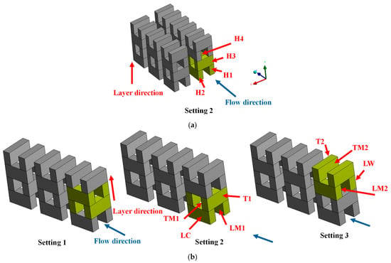
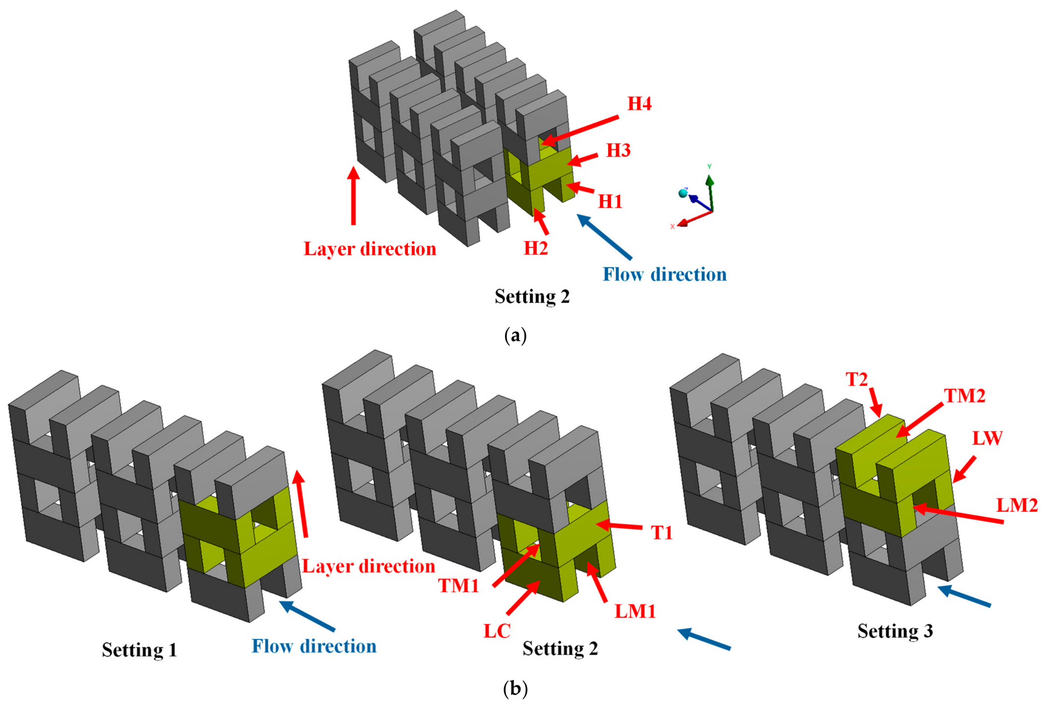
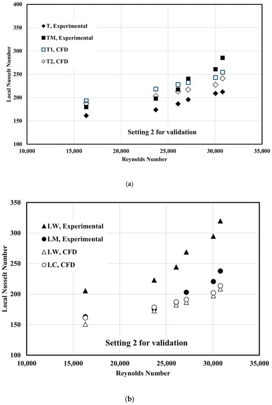
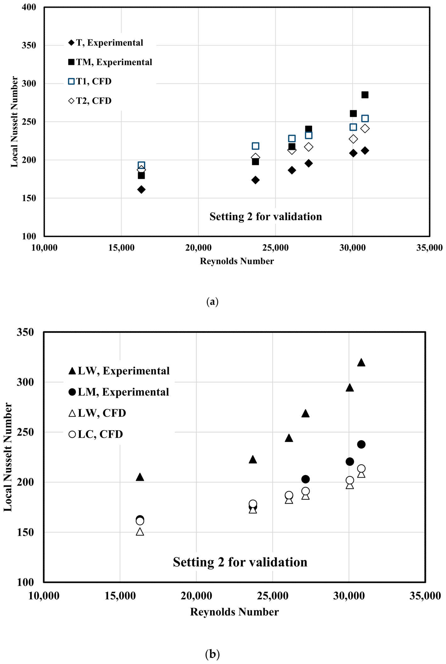
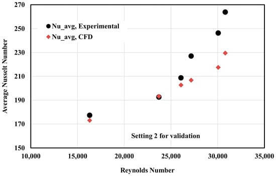
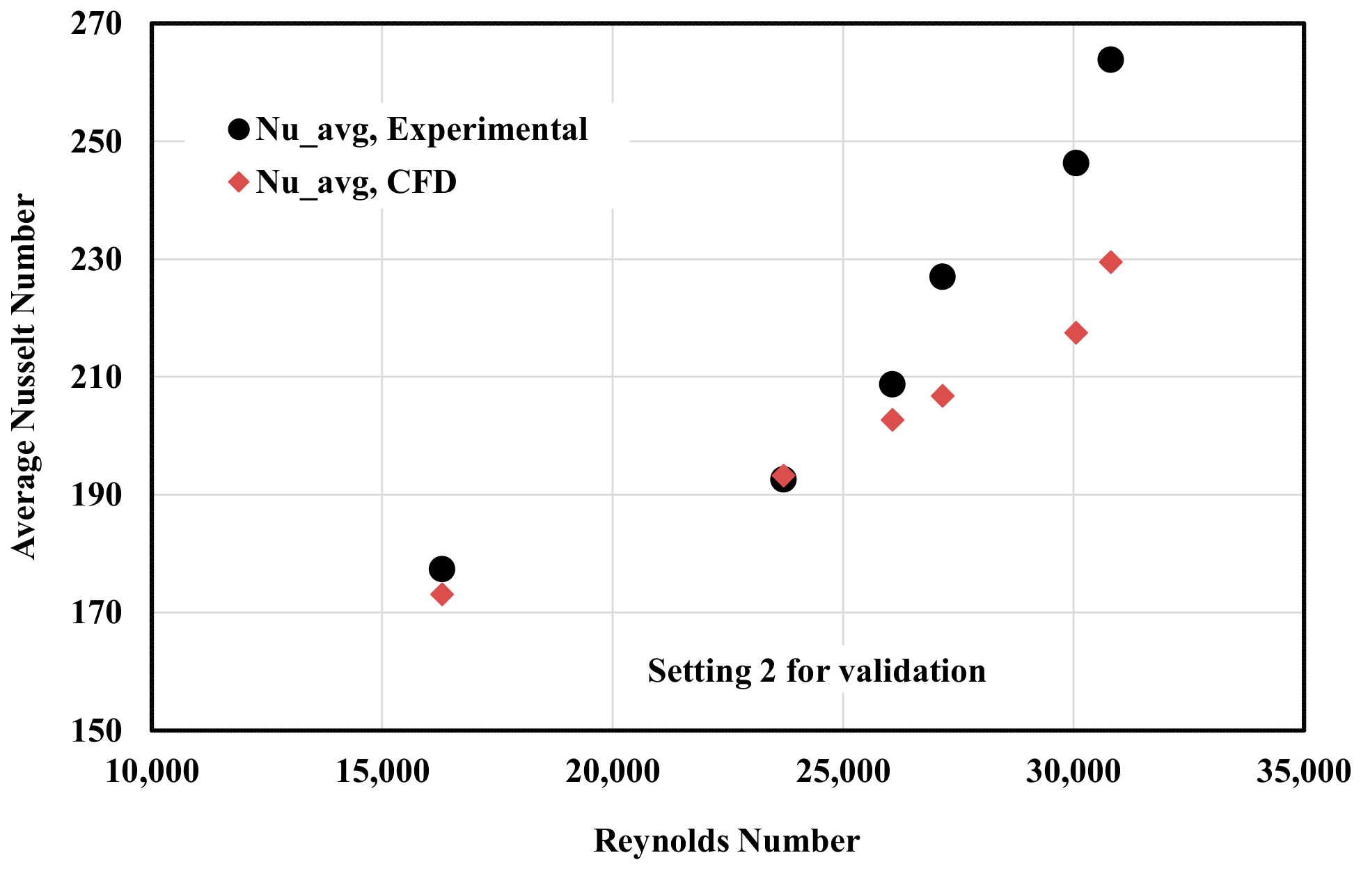
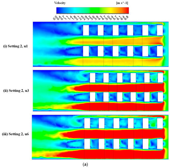
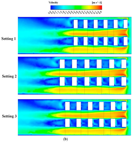
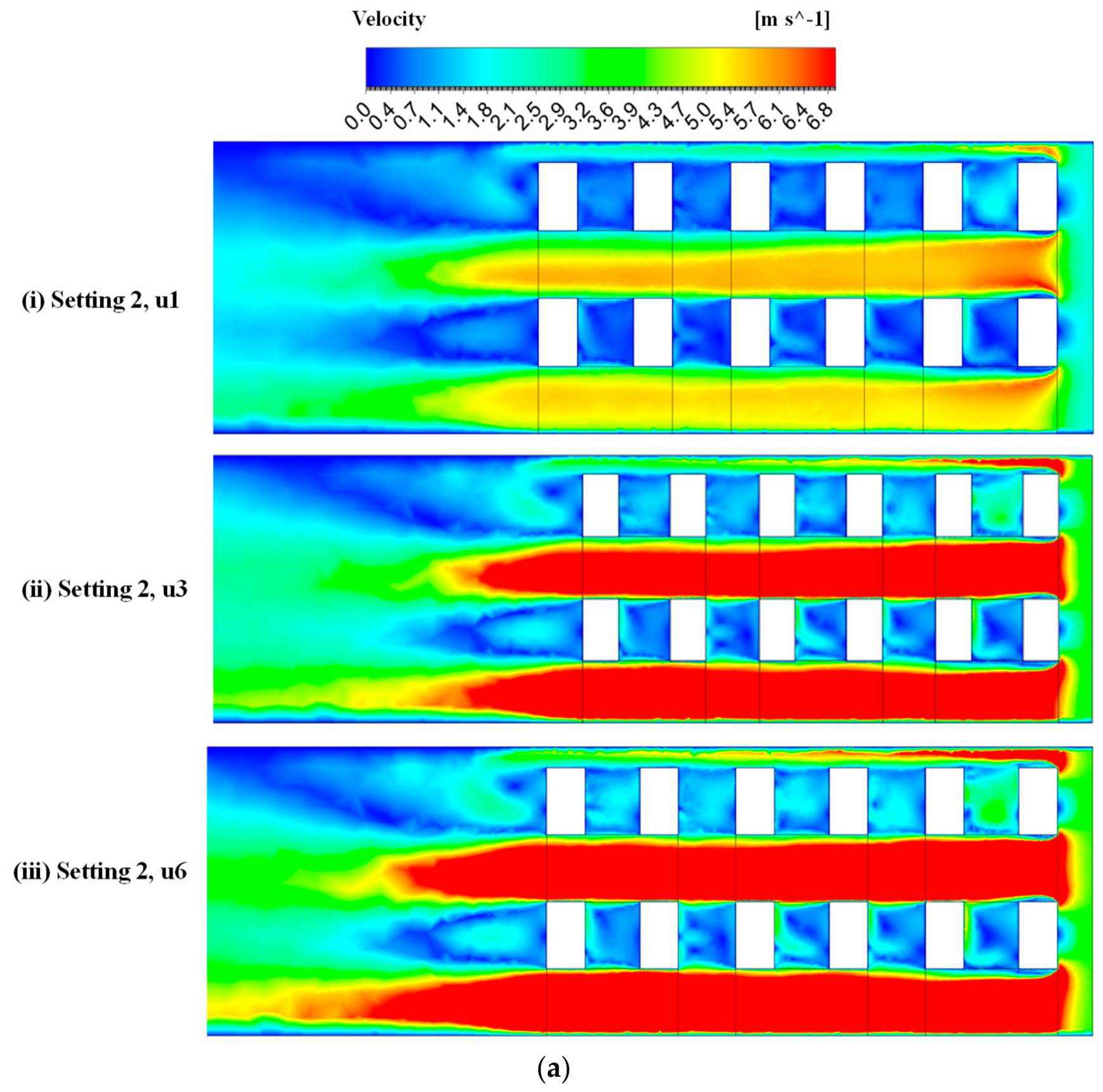
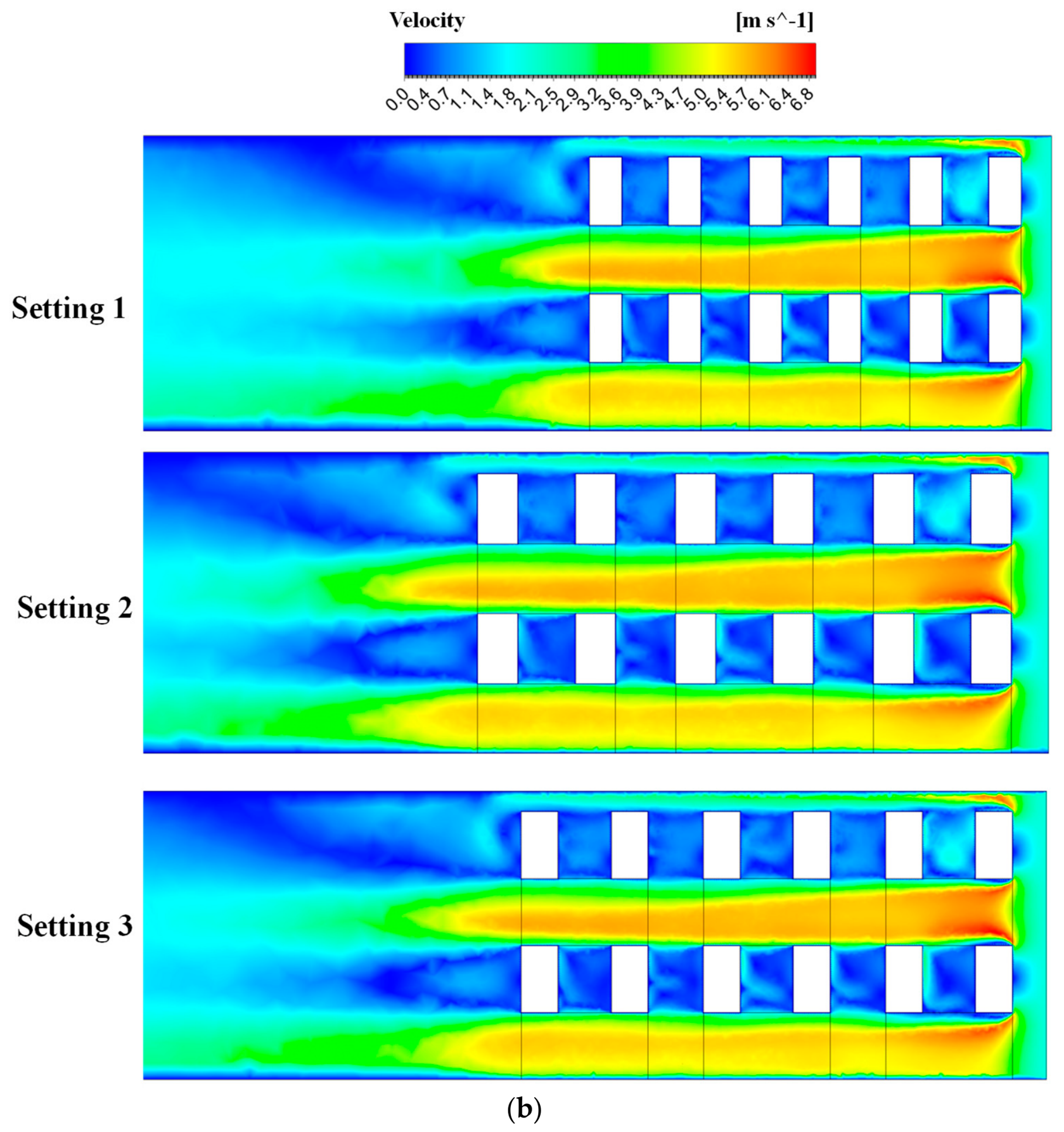
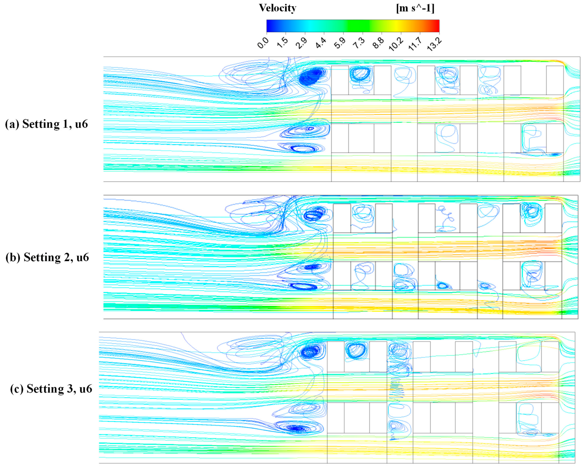
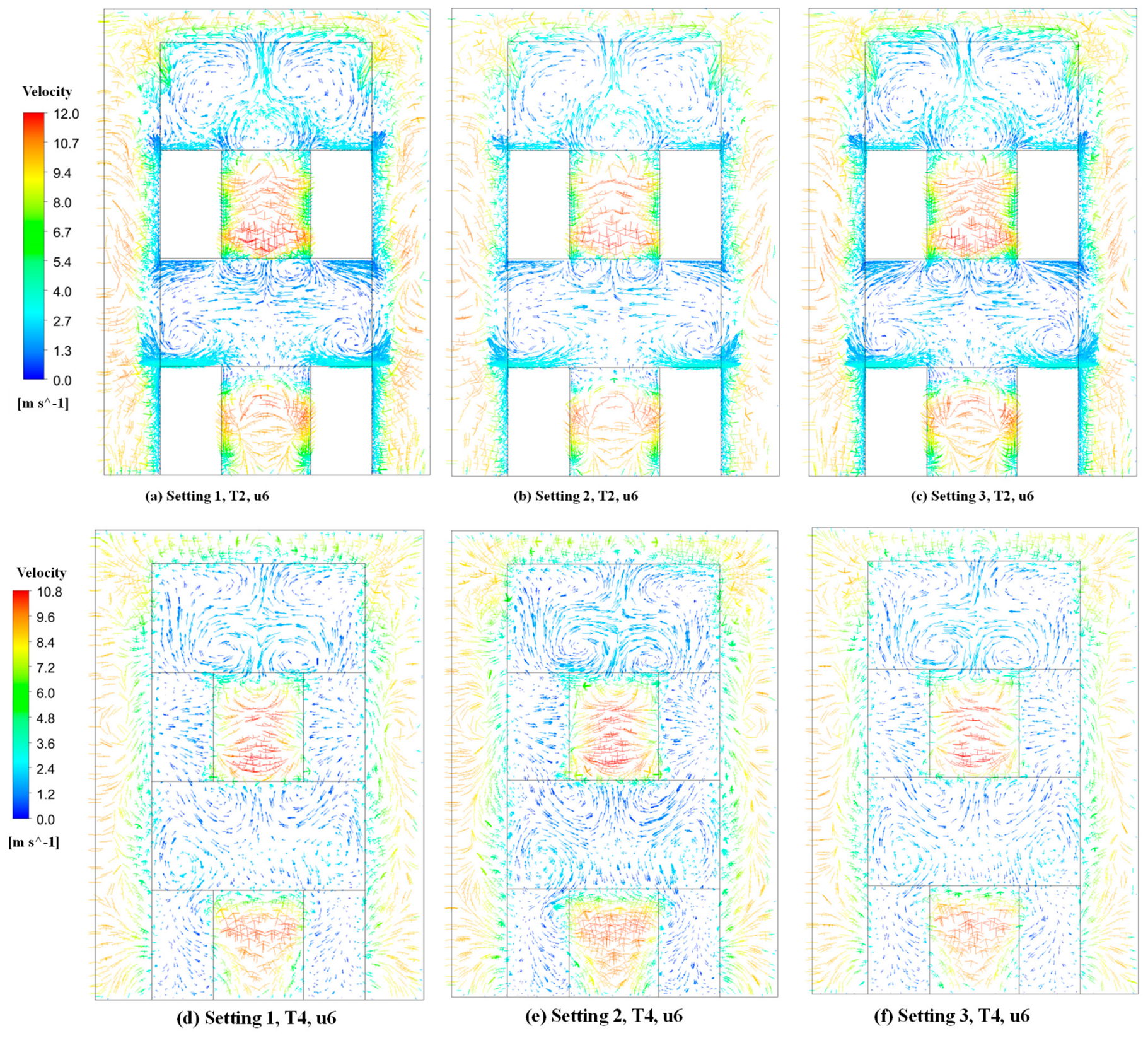
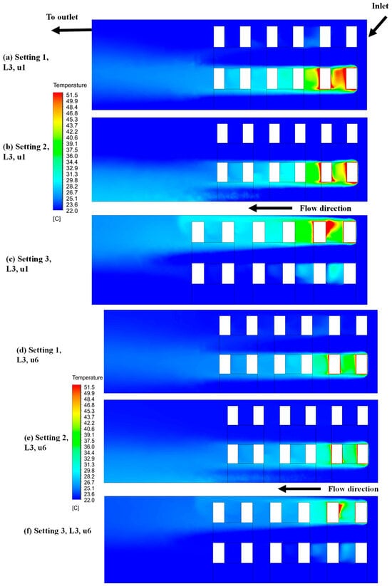
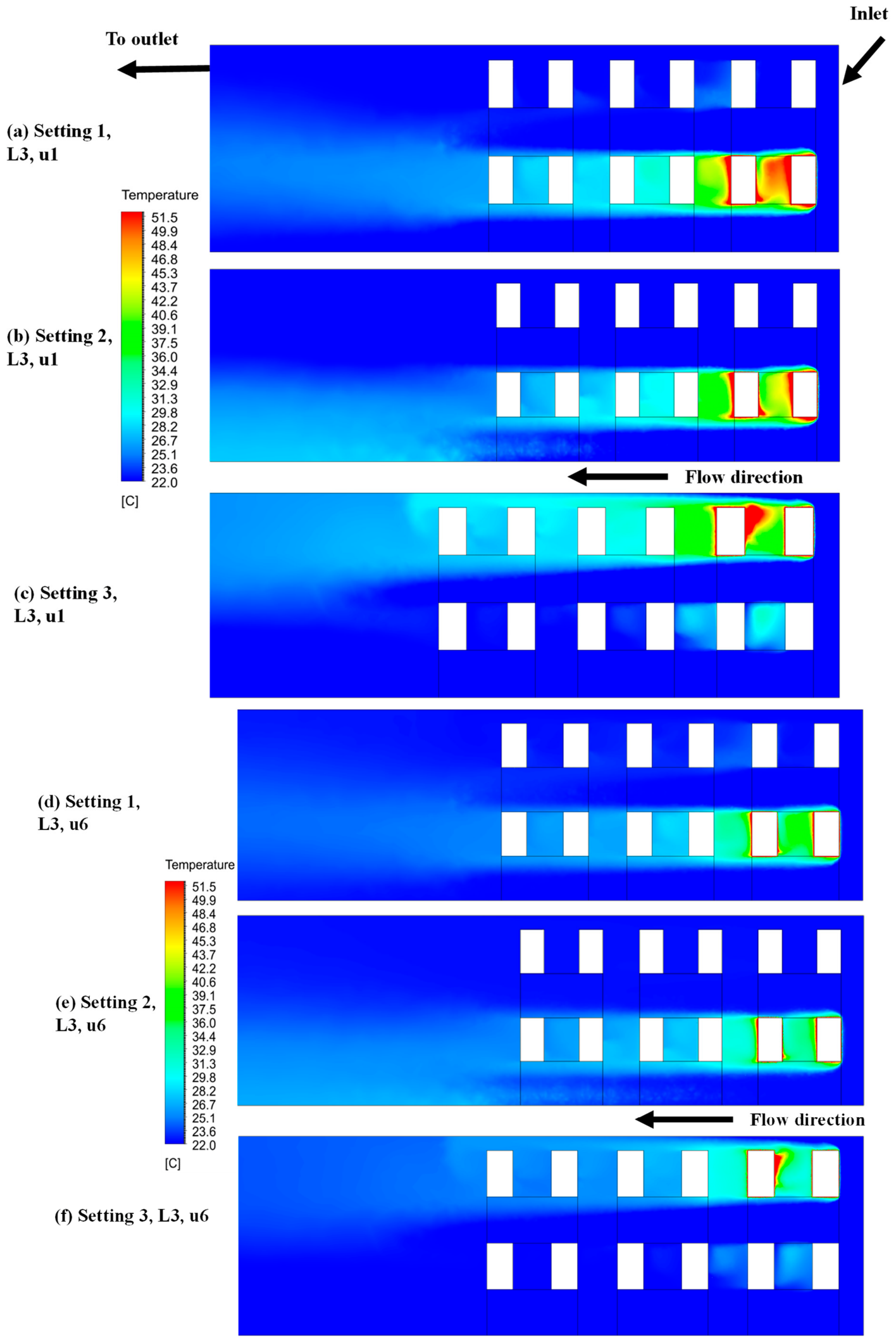
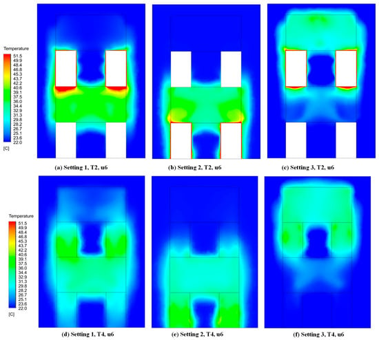
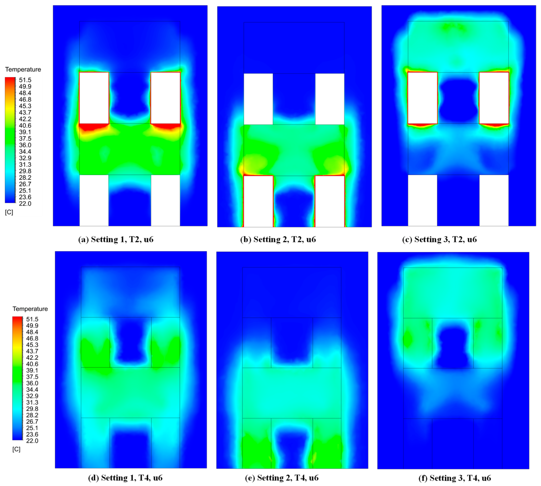
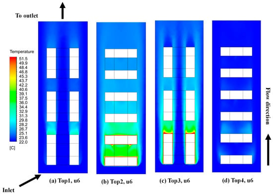
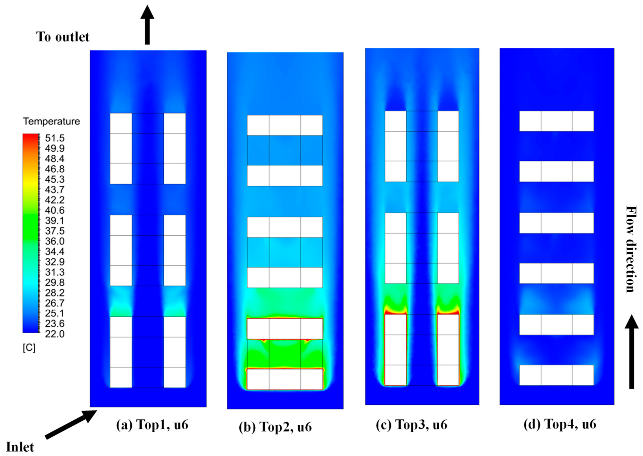
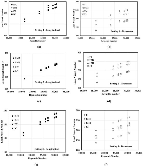
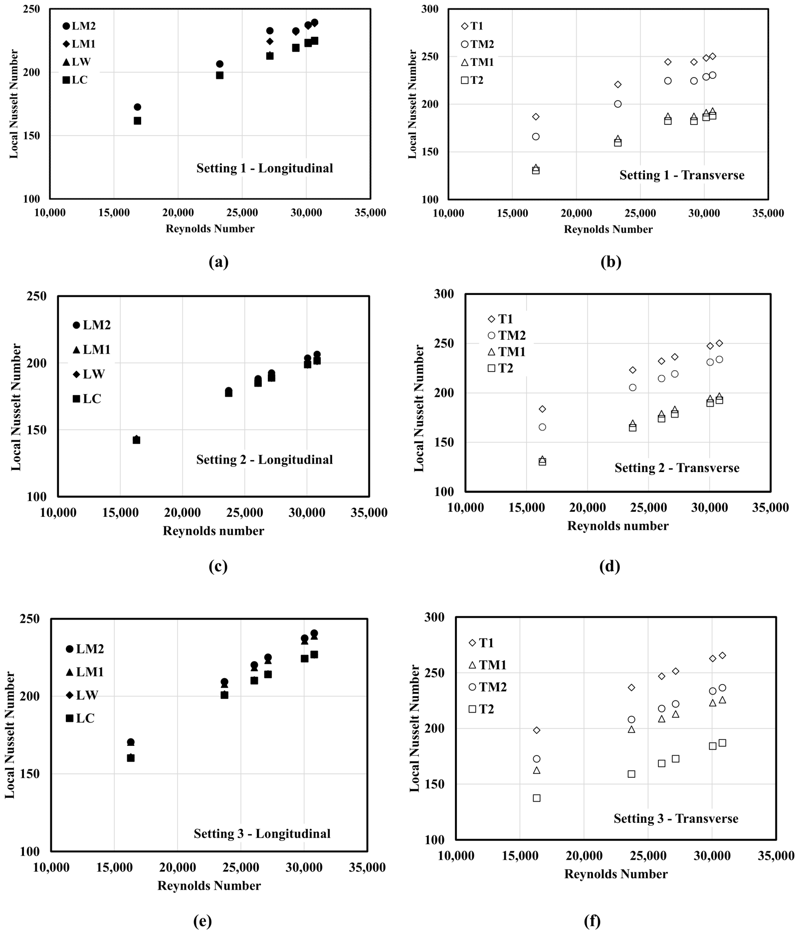
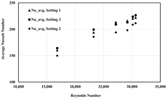
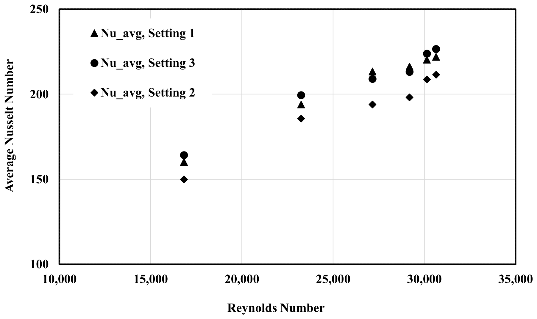
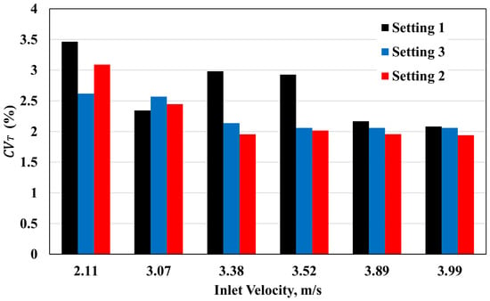
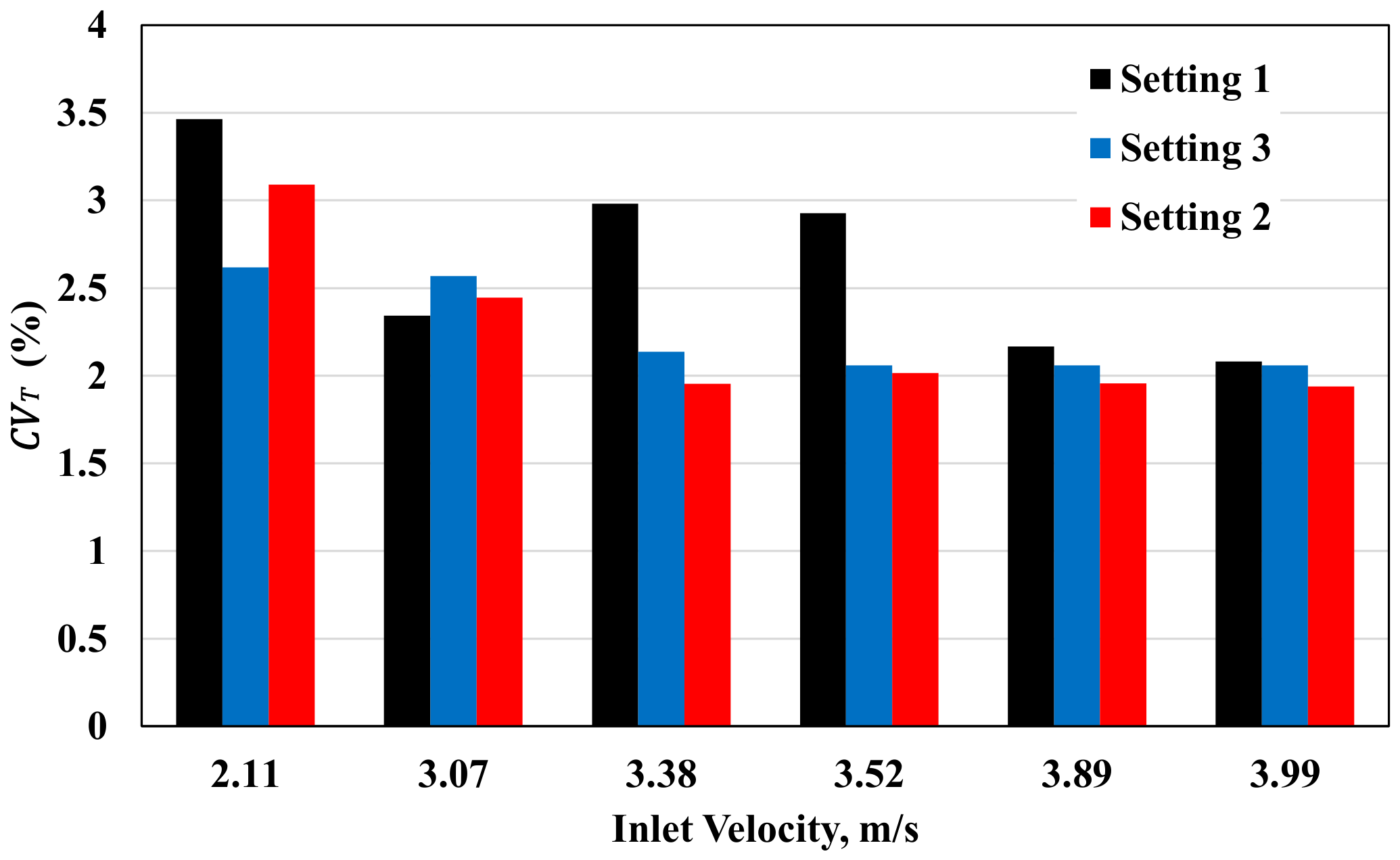

Disclaimer/Publisher’s Note: The statements, opinions and data contained in all publications are solely those of the individual author(s) and contributor(s) and not of MDPI and/or the editor(s). MDPI and/or the editor(s) disclaim responsibility for any injury to people or property resulting from any ideas, methods, instructions or products referred to in the content. |
© 2026 by the authors. Licensee MDPI, Basel, Switzerland. This article is an open access article distributed under the terms and conditions of the Creative Commons Attribution (CC BY) license.