


Abstract
The Ecuadorian electrical system, with a generation mix dominated by hydroelectricity, experienced prolonged rationing during recent droughts, prompting a search for generation options that can be installed near consumption centers. Before authorizing new connections, it is necessary to determine the capacity of the subtransmission network for distributed generation and whether this limit depends on the installed technology. This study addresses the integration of renewable energy systems into the 69 kV network of the Centro-Sur Regional Electric Company (CENTROSUR, Ecuador). Hourly wind and photovoltaic energy profiles were considered at eight candidate busbars, and the coordinated integration capacity of the system was determined by simultaneously injecting power into all of them. Six configurations with equal incoming power (renewable, thermal, and three mixed) are compared using power flows, N-1 contingencies, short-circuit analysis (using the full method), and RMS transient stability analysis with the support of the DIgSILENT PowerFactory tool. Five operating points are analyzed: two full dispatch points and three extracted from the year’s chronological data based on hourly solar and wind resource availability. The overall results show that the limit is set by a shared export corridor, not the bus connection point. The coordinated capacity is 160 MW at peak demand and 60 MW at minimum demand, compared to the 620 MW and 380 MW, respectively, that would result from adding the individual capacities of each bus. The operating point governing incoming power is the export condition, which occurs during an hour of intermediate demand with high local generation, not during peak or minimum demand. The sizing procedure is potentially applicable to other meshed subtransmission networks fed from a few points of the transmission system, a situation that can be replicated in other parts of the world.
1. Introduction
Electrical systems highly dependent on a single primary resource are vulnerable to extreme conditions affecting that resource. The Ecuadorian case illustrates this: a generation matrix dominated by hydroelectric plants exposed the country to prolonged rationing during recent droughts, prompting a search for backup generation that can be quickly deployed near consumption centers [1,2,3]. International experiences with emergency generation, such as floating plants, temporary thermal units, or islanded grid sections, show that the location and sizing of these reinforcements determine their effectiveness as much as their installed capacity [3,4,5,6]. At the same time, market mechanisms and demand management that value resources activated in contingencies complement, but do not replace, physical grid reinforcement [2,7,8,9].
In subtransmission networks, the integration of distributed generation (DG) modifies flows, voltage profiles, short-circuit levels, and the system’s dynamic response, with effects that can be favorable or adverse depending on the connection point and load status [10,11,12]. The literature on renewable energy integration documents both the improvement of voltage profiles with local injection [10,13] and the overvoltage and export problems when generation exceeds the local load [14]. Reactive power compensation coordination and redispatch in interconnected systems, studied for the Ecuadorian case in [15,16], confirm that resource location is crucial for voltage security.
A comparison between generation technologies also requires representative dynamic models. Generic WECC models of photovoltaic and wind power plants, simulated in DIgSILENT PowerFactory, were used [17,18], allowing for the representation of the limited current input of the converters and their power control, while synchronous machines are modeled using IEEE standards for machines and excitation systems [19]. At the regulatory level, the Ecuadorian Connection Code requires verification of the short-circuit ratio (SCR) at the connection point of all new generation [20].
This work systematically evaluates the integration of renewable and thermal generation into the 69 kV subtransmission network of the Centro Sur Regional Electric Company (CENTROSUR), which serves the provinces of Azuay, Cañar, and Morona Santiago. The projected hourly load and generation profiles for 2025 are applied to the DIgSILENT PowerFactory network model. Candidate busbars are identified using an annual low-voltage frequency criterion combined with sensitivity analysis (∂V/∂P and ∂V/∂Q) evaluated under extreme operating scenarios of an 8760 h annual sweep [3,6,10]. Three induction scenarios with identical total power are compared across the eight selected busbars: renewable (S1), thermal (S2), and mixed (S3) in three sub-cases against the base case without induction (S0).
The main objective of this work is to determine the maximum distributed generation capacity that the 69 kV subtransmission network of the CENTROSUR Electric Company of Cuenca-Ecuador can accommodate and to establish whether this limit depends on the technology used. Annual hourly analysis and sensitivity studies define where to connect; coordinated capacity defines the capacity; power flows and N-1 contingencies verify this limit under steady-state and safe operating conditions; and short-circuit and transient stability studies determine whether the limit changes with the technology.
The study sequence from a procedural point of view is as follows: First, it creates a detailed technical model of the operational behavior and voltage profiles associated with the integration of renewable energy quotas. Second, it provides a rigorous analysis of the stability and transfer capacity of the regional electricity grid under scenarios of high penetration of distributed and conventional generation. Finally, it offers a strategic planning tool, allowing for simulation using specialized software, which enables the distribution company to optimize its investments and guarantee the security and reliability of supply within its concession area.
The main contribution of this research lies in the systematic comparison of different renewable and thermal generation technologies connected to the subtransmission network, evaluating not only their generation capacity but also their effects on system operation. The analysis involves determining how technologies such as solar photovoltaics and wind power, compared to thermal alternatives, modify power flows, voltage levels, losses, and the operational stability of the 69 kV network. This methodological comparison is particularly relevant in the context of Ecuador’s energy transition, as a high incorporation of variable renewable generation can create new challenges related to active and reactive power management. Consequently, the research could establish technical criteria to determine which combination of technologies offers the best operating conditions and the greatest renewable integration capacity, providing decision makers with stronger arguments for considering future economic resources. Furthermore, this research can serve as a starting point for other applications in different geographical contexts before committing the inherently substantial economic resources.
Table 1 below presents the previous works that have been reviewed and that allowed this study to be outlined based on the new requirements that must be considered in the region.
Table 1.
Comparison with previous studies on distributed generation integration.
The analysis was performed using specialized Digsilent PowerFactory software (Version of 02/2026). This expansion allows for the evaluation of the robustness, reproducibility, and adaptability proposed in different scenarios, progressively reinforcing its applicability as a support tool for the planning and integration of renewable and thermal generation in subtransmission networks of the CENTROSUR Electric Company.
The remainder of the article is structured as follows: Section 2 describes the materials and methods. Section 3 presents the analysis for integrating renewable and thermal generation into the 69 kV subgrid of CENTROSUR. Section 4 presents the results and discussion. Finally, Section 5 presents the conclusions.
2. Materials and Methods
Figure 1 summarizes the methodology in eight stages. The first four correspond to the preparation of the study: gathering the technical data and the 2025 hourly profiles, building and validating the model in PowerFactory in Cuenca-Ecuador (ECU), identifying the candidate buses through the annual screening and the voltage sensitivities, and sizing the insertion from the local resource, the hosting capacity and the regulatory ceiling. The remaining four cover the analysis itself: the construction of the six cases with identical inserted power, the steady-state and N-1 assessment, the short-circuit and RMS stability studies, and the comparison that closes the work. Each stage feeds the next with a defined output, so that the differences observed between scenarios can be attributed to the technology inserted and not to the conditions of the study.
Figure 1.
Flowchart of the methodology followed in this study.
2.1. CENTROSUR 69 kV Network and Operating Data
The analysis system is the CENTROSUR subtransmission system, a 69 kV meshed network fed from two points of the transmission system, Sinincay (230 kV) and Cuenca (138 kV), studied in DIgSILENT PowerFactory 2024 [23]. The model comprises 106 buses (Table A1), 39 lines (Table A2), 39 two-winding transformers (Table A3), 21 three-winding transformers (Table A4) and 33 generation units (Table A5), whose complete characteristics are listed in Appendix A and in S2. The network is fed from the National Interconnected System (SNI) through the 138/69 kV interfaces of Rayoloma (CUE RAYO 138 transformers) and Sinincay and includes local hydroelectric (Saucay, Saymirín, Ocaña, Gualaceo, Alazán) and thermal (El Descanso) generation, grouped into 17 synchronous units. The projected hourly profiles for 2025 provided by CENTROSUR are applied to the model: 8760 h with load per substation and dispatch per generation unit. These are applied to the model hour by hour, verifying that the model’s demand matches that of the source file.
CENTROSUR provided the following information for this study:
- the projected hourly demand profile for 2025, with active and reactive power per substation for the 8760 h of the year;
- the projected hourly dispatch profile for 2025, with active and reactive power for each generating unit for the same 8760 h, including the four photovoltaic plants operating in the concession area;
- the subtransmission system model in DIgSILENT PowerFactory, with the electrical parameters of each element: 106 busbars, 39 lines with length, resistance, reactance, and nominal current, 39 two-winding transformers and 21 three-winding transformers with power ratings, transformation ratios, short-circuit impedance, and tap positions, and 33 generating units;
- the equivalents of the external 138 kV and 230 kV networks, with their maximum and minimum short-circuit power ratings.
Table 2 below presents the validation model with the representation adopted for each aspect.
Table 2.
Model validation: Representation adopted for each aspect.
Table 3.
Dynamic models used in the RMS simulation.
Figure 2 presents the network block diagram. The substations are connected by the 69 kV corridors, the SNI (National Interconnected System) entry point is located at Rayoloma/Sinincay, and the eight candidate buses for the new generation, selected in Section 3.1, are highlighted. Readers can identify the elements that dominate the results: the Cuenca–Ricaurte corridor and the interface transformers with the SNI, through which imports flow during peak demand and exports during minimum demand. The unfilled symbols denote open switches: they correspond to elements that are out of service in the base case provided by CENTROSUR, and were kept in that state to reproduce the actual operating configuration of the network.
Figure 2.
CENTROSUR 69 kV network and the SNI entrance (Rayoloma/Sinincay).
2.2. Mathematical Modeling
The four comparative studies are based on the classical formulation of power system analyses. The power flow solves the nodal balance of active and reactive power: at each bus i, the net power injected must equal the power flowing into the network, according to Equations (1) and (2).
where PGi and PDi are the generation and demand of the i-busbar, respectively; |Vi| y θij are the voltage magnitudes and the angular differences; and Gij and Bij denote the elements of the admittance matrix. The nonlinear system (1) and (2) is solved by the Newton–Raphson method, which in each iteration corrects the state vector with the Jacobian of the system, as in Equation (3):
Security criterion N-1 requires that, upon the individual departure of any element k from the network, the system remains within its operating limits. A contingency k is considered critical when it produces at least one new violation with respect to the case without contingency, that is, when it fails to meet any of the conditions of Equation (4):
where is the voltage at busbar i and is the loadability of branch b in the post-contingency. Short circuits are calculated using the full DIgSILENT method (superimposed on the actual operating point of each scenario) for both three-phase and single-phase-to-ground faults. The full method is preferred over the standardized IEC 60909 [11] calculation because it is based on the actual load condition and represents the limited fault contribution of inverter-based generators, which is relevant for renewable and mixed-use applications. From the initial short-circuit current Ik″, the short-circuit power and peak current are derived, as shown in Equations (5) and (6).
The complete method initializes the pre-fault condition with a power flow and superimposes the fault onto it, instead of starting from the standardized voltage profile used in the IEC 60909 calculation. This is the appropriate option here because it incorporates the dynamic voltage support of the connected generation via power electronics, whose contribution to the fault is not described by a subtransient reactance. The three-phase fault is resolved in the positive-sequence network and the single-phase-to-ground fault in all three sequence networks.
Converter-based units are represented with the dynamic voltage support model, which replicates the requirements of the connection codes. When the terminal voltage drop exceeds 0.1 pu, the unit injects a reactive current proportional to this drop through a factor K. The active current is reduced as needed so that the sum of both does not exceed the maximum permissible value, thus giving priority to the reactive component. In this model, the limit is 1.0 times the nominal current in the seven photovoltaic plants, which do not provide voltage support, and 1.1 times in the wind farm, with a K-factor of 2.0. These units do not contribute zero-sequence or reverse-sequence currents: their three-phase configuration cancels both components, and the step-up transformers, with a Dyn5 connection, place the delta on the 69 kV side, blocking the zero-sequence path to the grid.
The interface transformers with the national system have three windings with a YN0yn0d1 connection group, so the neutral is solidly grounded on the 69 kV side. This explains why, at some busbars, the single-phase fault current exceeds the three-phase fault current. For each bus, the initial symmetrical current Ik″, the short-circuit power S″k, the peak current ip, and the R/X ratio viewed from the fault point are recorded, both at maximum and minimum current and for both types of fault.
where Un is the nominal voltage of the faulted bus and κ is the crest factor, which depends on the R/X ratio seen from the fault point according to . Since the R/X ratio of each bus is reported, the peak current can be checked from the symmetrical initial current. With S″k, the Connection Code of regulation ARCONEL-001/24 [20] requires a minimum short-circuit ratio at each connection point (7), as follows:
The short-circuit ratio in Equation (7) is evaluated at each bus separately and assumes that the injection points are electrically independent. When several converter-based units are connected to the same system, this assumption no longer holds. A disturbance at one bus is transmitted to the others, and the actual robustness is lower than that indicated by the individual calculation. To quantify this coupling, the multi-infeed interaction factor is used, defined in Equation (8) as the ratio between the voltage variation that a reactive disturbance applied at bus i produces at bus j and the variation it produces at bus i itself. This indicator originates from the analysis of systems with several DC links on the same AC network and has been extended to injection points based on inverters, which exhibit the same coupling condition [24]. The integration guidelines for these resources acknowledge that the conventional indicator loses validity when several converters are electrically close [25].
The factor takes values between 0 and 1; they are close to zero when the buses are decoupled and close to one when they behave as a single connection point. It is used to weight the power injected at the other buses and obtain the effective short-circuit ratio of the multi-infeed system (9), where S″k,i is the short-circuit power at bus i and P is the installed power at each injection point. This is the formulation of [25], which is called MSCR, in its version without reactive compensation connected at the injection point, which is the one used in the model employed.
The MISCR is always less than or equal to the conventional SCR and coincides with it only when the coupling is zero. It is compared with the same thresholds: the minimum of 2 required by the Connection Code and the value of 3 that [25] sets as critical for this indicator when the connected generation is based on inverters. Below that value, the connection point is considered electrically weak.
is the installed capacity of the new generation at the bus. Finally, transient stability is evaluated using RMS dynamic simulation. The electromechanical behavior of each synchronous machine obeys the oscillation equation, as shown in Equation (10):
where H is the inertia constant, ωs is the synchronous speed, δ is the rotor angle, and Pm and Pe are the mechanical and electrical powers, respectively. Converter-based units do not have this dynamic. Their response depends on the inverter controls, which limit the current to 1.1 to 1.2 times the nominal current [17,18].
Equation (10) describes only the rotor motion. The effective dynamic behavior of each unit also depends on its speed governor and excitation system, which are included in the model; without them, the RMS simulation will not initialize. Table 3 identifies the model used in each case. Renewable units use the generic WECC models, studied in PowerFactory. For synchronous machines, however, neither ELECAUSTRO nor CENTROSUR has dynamic models of their generators, but rather their characteristics and unit test protocols. Therefore, the standard PowerFactory library models closest to the installed equipment were adopted and parameterized with this information. None of the power plants in the system have a power stabilizer installed, so its absence in the model reflects the actual operating conditions and is not a simplification.
3. Analysis for the Insertion of Renewable and Thermal Generation into the 69 kV Subtransmission Network of CENTROSUR
3.1. Annual Screening and Identification of Candidate Busbars
Busbar selection combines two complementary criteria that together offer a stronger choice than either alone. The first is an annual frequency criterion. A Newton–Raphson power flow is executed automatically for each of the 8760 h of the year and, in each hour, the five busbars with the lowest voltage are recorded, accumulating a counter of occurrences per busbar. The busbars that appear most frequently in that group consistently present the lowest stress profile of the year, along with the number of hours below 0.97 pu and their annual stress statistics. This criterion identifies the weak busbars of the system without depending on a specific scenario [10].
The second criterion evaluates the effectiveness and feasibility of the injection over the two extreme operating scenarios of the year (the time of lowest and highest minimum voltage). An increase of 5 MW and 5 MVAr is independently injected into each bus to determine the sensitivities ∂V/∂P and ∂V/∂Q, and the loading of adjacent branches is analyzed to establish the margin available to export the power. A busbar is ideal when it combines high voltage sensitivity with a wide export margin. The intersection of both criteria (recurrently weak busbars that also respond well to injection and have hosting capacity) is the set of candidates on which the insertion cases are developed.
3.2. Allocation of Generation Technology According to Local Resources
The guiding criterion for assigning the renewable technology to each site is the available resource. Each site was characterized by its geographic coordinates, and the potential photovoltaic output (PVOUT, in kWh/kWp) was extracted from the Global Solar Atlas [26] and the average wind speed at 100 m from the Global Wind Atlas [27]. These points were then projected onto resource maps in QGIS to verify their correspondence with the terrain.
Figure 3 shows the solar resource map of the concession area with the eight candidate sites superimposed. Warm tones indicate higher potential photovoltaic output, and cool tones, lower output. All sites fall within the high Andean plateau, with potential outputs between 3.93 and 4.33 kWh/kWp, a difference of only 10% between the best and worst sites, meaning that photovoltaic generation is viable in any of them.
Figure 3.
Solar resource (PVOUT, kWh/kWp) in the CENTROSUR concession area, with candidate busbars superimposed. Source: Global Solar Atlas [26].
Figure 4 presents the equivalent map of average wind speed at 100 m. Unlike solar, the wind resource is highly uneven. Most of the busbars are located in areas with moderate or low winds, and only Cañar falls within the high-wind corridor of the exposed plateau of the canton, with an exceptional value of 12.99 m/s. Therefore, wind power generation is allocated only to Cañar, and the other seven busbars are covered by photovoltaic generation.
Figure 4.
Average wind speed at 100 m in the CENTROSUR concession area, with candidate busbars superimposed. Source: Global Wind Atlas [27].
The value of 12.99 m/s corresponds to the Global Wind Atlas at a height of 100 m at the exact coordinates of the Cañar busbar, located on an exposed hill in the paramo. This wind regime is of the same order of magnitude as that of wind farms operating in the Ecuadorian highlands, making it plausible. Even so, to avoid relying on a single value from a global atlas, wind power is dispatched according to the hourly profile described in Section 3.7, whose annual capacity factor, based on the 20 MW dispatched at the busbar, is 45%. A project decision would require an on-site measurement campaign. The technology allocation was made solely based on available resources, because the objective of this work is the technical evaluation of the network; the levelized cost of energy, land availability, fuel supply logistics, emissions, supply reliability, and environmental or land-use restrictions were not considered, and all of these would influence a real investment decision. Incorporating these factors into a multi-criteria evaluation would allow the six configurations to be ranked by more than just their grid performance. Table 4 summarizes the resource per busbar and the assigned renewable technology.
Table 4.
Solar and wind resource per candidate bus and assigned renewable technology [26,27].
3.3. Insertion Scenarios and Dynamic Models
The insertion is modeled with two additional networks coupled to the candidate buses: a renewable network (the Cañar wind farm with 10 type 4A wind turbines rated at 2.5 MVA each and seven photovoltaic plants of 25 MVA, all with the generic WECC models in PowerFactory [23]) and a thermal network with eight synchronous units GT1-GT8 of 21 MVA. Each bus has a renewable unit and a thermal unit, and the scenarios are built by switching units on and off using PowerFactory operating scenarios, without modifying the topology. Synchronous generator sets are represented using a composite model of machine, governor, and excitation compliant with IEEE standards [19]: existing hydroelectric plants with the governor gov_IEEE_Hydro2 (which includes the water start-up time Tw), the El Descanso diesel plant and the inserted thermal generator sets with gov_IEEE_GGOV1, recommended by NERC for gas and diesel generator sets, and all generators with the static excitation exc_IEEE_ST1A, consistent with the Basler DECS digital controllers installed at ELECAUSTRO’s plants.
Each of the eight busbars receives a dispatch of 20 MW. The Cañar wind farm is modeled with ten 2.5 MVA wind turbines. The photovoltaic plants and the wind farm are represented in aggregate using the generic WECC models incorporated in DIgSILENT PowerFactory. Aggregate representation is standard practice for power plants composed of numerous small-scale units. Table 5 shows the dispatch assigned to each busbar and the capacity of its connection transformer.
Table 5.
Connecting transformers of the inserted generation.
All the incoming generation is dispatched without reactive power input across all three technologies. This is the most conservative assumption regarding voltage support. The Connection Code requires new power plants to have reactive power regulation capacity, so enabling it would improve the voltage profile and increase capacity. The limits determined by the voltage profile are therefore a conservative estimate; the thermal constraints of the grid corridor and the dynamic results governed by the active power balance do not necessarily improve proportionally. The study does not model the reactive power control method of the units, the definition of which corresponds to the interconnection study for each plant.
Each bus receives 20 MW across all three technologies, which defines the 160 MW incoming capacity and makes the configurations comparable. The connection transformers are specified above this value, with a margin of approximately 20%, so that the connection equipment does not limit injection or introduce overloads unrelated to the phenomenon being studied. At maximum dispatch, their load capacity is between 79% and 84%. The step-up transformers for the thermal units were resized from 20 to 24 MVA. With the transformer’s capacity equal to that of the machine, the unit would have driven it to 100% capacity when dispatching its nominal power, without the margin required by an interconnection specification, see Figure 5.
Figure 5.
Single-line diagram of the system with the inserted renewable generation (S1 configuration): 20 MW in each of the eight candidate buses, photovoltaic in seven of them and wind in Cañar.
Six case studies with identical incoming power are defined. The base case S0 represents the grid without new generation. S1 adds 160 MW of renewables (the Cañar wind farm and seven photovoltaic plants); S2 adds 160 MW of thermal power (GT1–GT8); and S3 combines both technologies in three subcases. The requested renewable energy percentages (approximately 80, 50, and 30%) are studied in uniform 20 MW blocks, with achievable proportions that are multiples of 12.5%, resulting in 75%, 50%, and 25% renewable energy: S3-80, S3-50, and S3-30, respectively. The criteria for deciding which busbars are converted to thermal power are outlined in Table 4; thermal power first replaces the busbars with the worst solar resource (S/E 13, with 3930 kWh/kWp, and Lentag, with 3938 kWh/kWp), while maintaining the renewable energy where the resource is better (Az and EEAz2, with 4327 kWh/kWp). Table 6 details the allocation. With this construction, S1, S2 and the three subcases of S3 insert exactly the same 160 MW, so that the differences observed in voltages, loadings, losses, contingencies, short circuits and stability are attributed to the nature of the generation (converter or synchronous machine) and its proportion, not to the penetration level, see Figure 6. The tomato-colored line appears because it is disconnected in all cases.
Table 6.
Subcases of the mixed scenario S3: technology allocation per bus (20 MW blocks). The percentages refer to the renewable share of the installed inserted capacity, not to the instantaneous renewable generation.
Figure 6.
Single-line diagram of the system with thermal generation inserted (S2 configuration): 20 MW of synchronous generation at each of the eight candidate buses.
The three S3 subcases are obtained using these same schemes, activating either the renewable or thermal unit at each busbar according to the distribution in Table 6, without modifying the topology or connection points. Therefore, they do not require their own diagram.
3.4. Evaluated Operating Points
The study evaluates two sets of operating points that address different questions. The first set comprises full dispatch scenarios: the maximum and minimum annual demand with all generation operating at its nominal capacity. These are stress tests, not actual time-based conditions (there is no photovoltaic production at 7:00 PM). Their purpose is to define the theoretical limits of the grid. The maximum import relief that the grid connection can provide and the maximum export demand it can impose. The grid’s capacity is derived from these tests.
The second set comprises actual time-based points, where demand, existing generation, and solar and wind resources correspond to the same time of year. The study’s conclusions are drawn from these points. Three are distinguished, and none replaces the others: the hour with the highest renewable energy participation, the most electrically demanding hour among those with significant renewable energy presence, and the most electrically demanding hour of the entire analyzed set, regardless of the technology used. Table 7 defines these points.
Table 7.
Evaluated operating points: Definition, selection criteria and purpose.
The separation between C2 and C3 is deliberate. C2 addresses the temporal overlap of solar and wind resources with demand, and by design excludes nighttime hours, when photovoltaic contribution is zero. C3 does not apply any restrictions on the resource and incorporates the most demanding condition of the set, which can arise during a period of low irradiance with intermediate demand and high local dispatch. Presenting only C2 would obscure this condition; presenting only C3 would leave the temporal overlap unaddressed. A threshold of 70% is used for C2, with a sensitivity analysis at thresholds of 60% and 80%.
In all five points, the integrated thermal generation is maintained at nominal power. This assumption represents its maximum firm contribution and not necessarily the economic dispatch. Thermal generation is dispatchable and can be reduced through redispatch, while renewable generation depends on the resource and any excess can only be managed through reduction, storage, or export.
The dates and times for C1, C2, and C3 are selected from the analyzed set of time conditions and identified using power flow data. All three points are applied at the same date and time to the six configurations, ensuring that the technologies are compared under the same demand and dispatch conditions for existing generation. C1 corresponds to November 1st at 11:00 AM, with a renewable generation-to-demand ratio of 0.964. The peak absolute renewable production time is different: September 21st at 12:00 PM, with 138.4 MW; C2 corresponds to January 25th at 12:00 PM; and C3 to January 19th at 8:00 AM.
3.5. Sizing of the Inserted Generation
Comparing scenarios requires first establishing two things: the network conditions under which they are compared and the power allocated to each busbar. The network conditions were obtained by processing hourly profiles from 2025 to identify characteristic times of the year. Peak demand occurs on September 30 at 7:00 PM, with 219.5 MW supplied, of which 68.4 MW are generated locally, and 154.7 MW are imported from the National Interconnected System (SNI) through the 138/69 kV interfaces. Lowest demand falls on January 1 at 8:00 AM, with 73.8 MW supplied locally, 75.9 MW generated locally, and a near-zero exchange of 1.5 MW. The studies are conducted on these two complementary operating points: maximum demand (Dmax) is the condition of highest annual load and the one in which new generation can provide the greatest import relief, while minimum demand (Dmin) governs export capacity, because with local load at its minimum, the injected power must be evacuated through the grid.
These values correspond to simulated operation and differ slightly from the gross totals of the hourly profile, which schedules 228.0 MW at peak and 77.9 MW at off-peak. On the demand side, the EEAz and Guapán buses are not energized (their feeder SE09-EEAz1 is out of service, leaving 5.9 MW unserved), and the EEAz2 load has a scaling factor of 0.70. On the generation side, dispatch at minimum demand differs from the profile because four photovoltaic plants in the profile are not represented as dispatchable units in the model. At peak demand, at 7:00 PM, these plants do not generate, and both values coincide at 68.4 MW.
The power allocated to each bus was determined by an automated incremental sweep on the PowerFactory model, which calculates the maximum permissible injection at each candidate bus (accommodation capacity). Active power is injected at each bus in 2.5 MW steps, with a unity power factor (a conservative criterion that does not provide reactive power support for the new generation), and a Newton–Raphson power flow is run at each step. The sweep stops at the first new violation with respect to the base case: a line or transformer above 100% load, a voltage outside the 0.95 to 1.05 pu band, or non-convergence of the power flow. The accommodation capacity is the last injection without violations, and the limiting factor is recorded.
The results (Table 8) confirm that the governing case is the minimum demand. At peak demand, only Substation 13, Cañar, and Corpanche reach a limit: Substation 13 at 70 MW and the other two at 75 MW. The remaining buses exceed the 80 MW sweep limit because local injection displaces imports and relieves the Cuenca–Ricaurte corridor and interface transformers, which operate under overload conditions (T213 at around 146% and CUE RAYO 138 at 112%). At minimum demand, the limit appears earlier and almost always due to overvoltage at adjacent medium-voltage buses, not due to load capacity. This is typical behavior for a network with high injection and low local load. The most restrictive bus is Lentag, with 22.5 MW.
Table 8.
Hosting capacity per candidate busbar and limiting element at both operating points.
100% of the continuous nominal capacity is adopted as the limit for three reasons: it is the planning criterion used by the operator to authorize new connections, since Article 12 of the Connection Code requires compliance with the permissible currents under steady-state conditions and reserves the temporary overload regime for system failures [20]; it does not allow for temporary overload capacity, because this is reserved as a margin for contingencies; and it makes the six scenarios comparable. The system transformers allow for emergency overloads in accordance with IEC 60076-7, on the order of 130% for limited periods and depending on the ambient temperature and the previous load, so the reported load capacities do not imply an immediate failure condition but rather the exhaustion of the planning margin. The condition following a contingency is evaluated separately in Section 4.3. The capacity sweep is deliberately performed in the N-0 condition to separate the connection point’s own limit from the limit imposed by safety in the event of a contingency.
3.6. Coordinated Accommodation Capacity
The bus-by-bus capacity calculation assumes that injection occurs at a single point, whereas the scenarios in this work connect 20 MW across eight buses simultaneously. Because the injections interact with each other, the incremental sweep was repeated by injecting simultaneously at the eight candidate buses, in 2.5 MW increments per bus, until the first new violation compared to the base case. Table 9 presents the results.
Table 9.
Individual versus coordinated accommodation capacity in the eight candidate bars.
The bus-by-bus analysis overestimates the actual limit by a factor of four to six because it ignores the electrical coupling between injection points. This figure quantitatively explains the export overload reported in Section 4.2. The 160 MW inserted are equivalent to 2.7 times the coordinated capacity of the entire system at minimum demand. A non-uniform allocation, proportional to the individual capacity of each bus and scaled up to the first violation, was also tested; the total allowable allocation is identical to that of the uniform allocation, demonstrating that no bus-by-bus allocation can improve the result as long as the active constraint is the shared corridor. Therefore, the uniform dispatch of 20 MW per bus is no longer an assumption; it coincides with the coordinated capacity at maximum demand, respects the most restrictive bus, and corresponds to the commercial size of the modeled units.
In addition to the capacity requirements, there is a regulatory ceiling. The Connection Code of regulation ARCONEL-001/24 requires a short-circuit ratio greater than 2 at the connection point [20], which limits the installable power per busbar to half its short-circuit power S″k in the base case, according to Equation (7) of Section 2.2. The lowest ceiling is found in Lentag, with 155.0 MW (S″k = 310.1 MVA), and the highest in S/E 17, with 483.6 MW. This criterion does not impose any restrictions on the unit sizes considered, from 20 to 25 MVA.
With these elements, the dispatch per busbar is set at 20 MW, the minimum among the three criteria: the capacity of the worst-performing busbar (22.5 MW in Lentag, which defines the order of magnitude), the nominal power of the modeled units (20 MW from the thermal unit, a wind farm with ten 2.5 MVA units, and a 25 MVA photovoltaic plant), and the ceiling capacity for SCR (155.0 MW, with no effect). The eight busbars total 160 MW, equivalent to 73% of the maximum demand and slightly above the total import during peak hours. The photovoltaic dispatch is also set at 20 MW, out of the 25 MVA installed, to maintain the same penetration across all technologies and make the scenarios comparable.
3.7. Resource Time Profiles and Selection of Chronological Points
Points E1 and E2 dispatch the connected generation at its nominal power, a hypothesis that limits the maximum impact but does not correspond to any actual time. At 7:00 PM, when the system reaches its peak demand, there is no photovoltaic production. To construct the time points, the solar and wind resources were incorporated hour by hour at each candidate busbar.
The specific photovoltaic production series were obtained from the PVGIS service of the Joint Research Centre of the European Commission, for the coordinates of each of the seven solar busbars, and the wind generation series for the Cañar area was obtained from the NASA POWER hourly base, adjusted to the Global Wind Atlas resource. All series are referenced to local time, the same as the demand profile, and correspond to a representative year of the available period. The hourly details are included in S7.
Figure 7 shows the result. Photovoltaic production is concentrated between 7:00 and 18:00, with a maximum average capacity factor close to 49% at midday, and is zero at 19:00 on all days of the consulted record. The annual capacity factor of the seven photovoltaic arrays varies between 13.1% in Corpanche and 16.3% in Descanso, equivalent to a specific production of 3.14 to 3.91 kWh/kWp per day, consistent with the solar resource values shown in Table 4. The wind resource in Cañar presents a different profile, with an annual capacity factor of 45% and a morning peak, partially complementing the solar resource. The tomato-colored curves represent possible operating scenarios for the photovoltaic system.
Figure 7.
Average hourly plant factor of the solar resource in the seven photovoltaic bars and of the wind resource in Cañar. The thin lines are the individual profiles of each of the seven photovoltaic busbars, and the thick line with markers is their average.
Applying these factors to the 20 MW installed at each bus yields the power that each configuration can inject at each point of operation, as shown in Table 10.
Table 10.
Power actually injected per configuration at each point of operation, out of the 160 MW installed.
Figure 8 shows what happens during peak hours. The renewable energy configuration injects no power during this time and is indistinguishable from the baseline scenario: the photovoltaic system produces no energy, and the wind farm is idle. The mixed configurations contribute only their thermal component, and only the thermal alternative injects the full 160 MW. At peak resource times, the relationship is partially reversed. At C1, the renewable energy configuration injects 127.9 MW, just 32 MW less than the thermal configuration.
Figure 8.
Power injected by configuration at peak demand time: full dispatch assumption versus the resource actually available.
Using the same resource, the number of hours per year for each configuration to export energy to the national grid is calculated. This figure defines the scope of the restriction and is shown in Table 11.
Table 11.
Hours of the year with net export to the national system, out of the 8760 evaluated.
The full dispatch assumption places exports for all hours of the year in all five configurations. With the actual resource, the renewable configuration exports for 13.1% of the year, and the thermal configuration for 100%, because it is the only one whose power output does not depend on the resource. Net exports appear in all five configurations, but their temporal scope differs by a factor of seven.
The busbar series also quantifies the correlation between photovoltaic plants. The correlation coefficient between pairs of plants, calculated based on resource-available hours, averages 0.727, with a minimum of 0.607. The plants are therefore strongly correlated (the concession area covers approximately 60 km2 and shares a cloud cover regime), but they are not identical. This justifies treating their production as simultaneous, which is what the model does, and at the same time limits the diversification margin that could be expected from a wider geographical distribution.
Based on these profiles, the three time points defined in Table 7 were selected. C1, the hour with the highest renewable energy participation, corresponds to November 1st at 11:00, with 127.9 MW of renewables versus 132.8 MW of demand, a ratio of 0.964. The hour of maximum absolute renewable energy production is different: September 21st at 12:00, with 138.4 MW. C2, the most electrically demanding condition among the hours when renewable generation reaches at least 70% of the annual maximum, corresponds to January 25th at 12:00. C3, the most demanding condition without resource constraints, corresponds to January 19th at 08:00. All three were identified with power flow data in the six configurations and are applied to all of them at the same date and time.
The selection of C2 depends on the adopted threshold, so its sensitivity was checked. With thresholds of 60% and 70%, the selected time remains the same: January 25th at 12:00, with a maximum load capacity of 152.4% at the interconnection transformer. With a threshold of 80%, the time shifts to July 27th at 11:00, and the requirement decreases to 144.7%, because the hours of highest irradiance are also those of highest local demand, resulting in a smaller exportable surplus. The 70% threshold is adopted because it is the value at which the resource is clearly high without the selection shifting towards less demanding conditions.
C2 and C3 do not coincide. The most demanding condition in the analyzed set occurs during a morning hour with intermediate demand, still-low irradiance, and high local generation, where the firm thermal component cannot be utilized, and not during an hour of high renewable resource availability. Restricting the analysis to the hours of high renewable presence would have underestimated the maximum requirement on the interconnection corridor by 34 percentage points.
3.8. Dynamic Events and Stability Criteria
Four representative events were configured, applicable to any scenario: (A) three-phase fault on the Cuenca–Ricaurte line, the most severe contingency identified in N-1, at 50% of its length at t = 1.0 s, cleared at 150 ms with line opening; (B) unexpected tripping of the CUE RAYO 138 transformer, i.e., loss of the main link with the National Interconnected System (SNI); (C) three-phase fault on the S/E 17-El Arenal line, which assumes the transfer when the Cuenca–Ricaurte line is lost; and (D) sudden loss of the 20 MW connected at Descanso, simultaneously tripping the photovoltaic unit and the thermal unit at that bus, so that in each scenario the unit in service operates and the same event compares the response with synchronous inertia or with a converter. In each simulation (12 s, balanced RMS step), 24 variables are monitored: the voltages of the eight connection buses, the speed, angle and power of the synchronous units, and the active and reactive power of the WECC units. A total of 23 simulations were run per programming interface: four events in each of the six configurations, except event D in the base case, which has no inserted generation to disconnect.
To these runs are added the four repeated events at the point of minimum demand, increasing the dynamic analysis from 23 to 46 simulations. Event B is extended to 30 s, recording the reactive power of the machines and external networks, the rotor angle, and the electrical frequency. The critical clearing time of the three-phase fault in Event A was determined by sweeping the clearing time across the six configurations.
A formal stability criterion is adopted and applied uniformly to all runs. A simulation is considered stable when, in the last three seconds, no machine in the coherent group deviates by more than 2% from its nominal speed, the relative angular opening between machines does not increase by more than 180 electrical degrees from its pre-disturbance value, and the voltage does not maintain a negative slope below 0.90 pu. The coherent group is identified by grouping the machines by their final speed, which separates the Morona Santiago area, fed radially, from the diagnosis, which, after the loss of the link with the national system, remains operating asynchronously with respect to the 69 kV ring.
The simulations demonstrate the behavior of the numerical model. Field validation will be carried out as future work on the actual CENTROSUR system network.
4. Results and Discussion
The results below summarize, for each scenario, the variables that govern the comparison. Greater detail on the development of the scenarios, the dispatch of every generator and every load, the voltage of every bus, the loading of every line and transformer, the complete list of N-1 contingencies, the short-circuit currents, and the RMS curves is reported in the Supplementary Materials to this research, which are listed at the end of the document and referenced in each subsection.
4.1. Identification of Candidate Busbars and Validation of Scenarios
The annual sweep runs through 8760 h of 2025 with an hourly Newton–Raphson flow, of which 8735 converged smoothly. The most demanding time of the year falls on 24 February at 11:00, when the minimum system voltage drops to 0.96259 pu at the EEAz2-69kV bus. The least demanding is 1 January at 08:00, with 1.00414 pu. Throughout the year, only 24 h (0.3%) left a bar below 0.97 pu, and the limit of 0.95 pu was never crossed. The system then operates within the band and the question is not where to correct the voltage, but rather where to connect the new generation.
The first filter is applied over the entire year (Table 12). Lentag-69kV leads in frequency of appearance among the five lowest-voltage bars, with 99.7% of the year, followed by S/E 13-69kV with 92.2% and Erco-69kV with 67.1%. EEAz2-69kV and Az-69kV-A appear less frequently, at 49.3 and 48.0%, respectively, but they accumulate the most hours below 0.97 pu and register the lowest minimum annual voltage.
Table 12.
Most frequent busbars in the group of the five with the lowest voltage and annual statistics.
The second filter measures the response of each busbar to injection during the two extreme hours of the year (Table 13). Alazán 69 is the most sensitive, with ∂V/∂Q = 0.004166 pu/MVAr, followed by Lentag-69kV and Saucay-69kV. In all of them, the reactive component dominates the active component, which is expected behavior in a subtransmission network. Adding to the sensitivity is the load capacity of the neighboring branches: Alazán, Lentag, S/E 13, and Saucay exceed the export margin of 88%, while the Macas-Abanico area remains under observation due to its link line, at around 57%.
Table 13.
Sensitivity and export margin of the highest-response busbars (worst scenario).
After applying both filters, a group of four busbars remains: Lentag-69kV, S/E 13-69kV, EEAz2-69kV, and Az-69kV-A, the latter corresponding to the Huablincay substation (S/E 09) in Azogues. These four appear recurrently among the weak busbars and simultaneously exhibit high sensitivity to injection with ample export margin. Alazán, Saucay, and Saymirín are excluded, despite their good response, because they already have their own 69 kV generation. Macas-Abanico is excluded due to the load capacity of its line. Descanso-69kV is retained because its generation is at 22 kV and does not interfere with 69 kV exports, and Cañar, Corpanche, and S/E 17 are added due to their margin and their presence among the lower voltage busbars. The eight buses in Figure 2 are, therefore, Lentag, Az, S/E 13, EEAz2, Cañar, Corpanche, Descanso, and S/E 17.
Each scenario created in PowerFactory was simulated with a power flow at the point of peak demand, measuring the effective contribution of the inserted units. (Table 14). The dispatches match the defined values: 160 MW in total in the five cases with insertion, and renewable proportions of 100, 0, 75, 50, and 25%. Insertion, with any technology, raises the minimum voltage of the candidate buses from 0.969 pu (Lentag at S0) to approximately 0.998 pu.
Table 14.
Validation of the scenarios: Measured dispatch of the inserted units (maximum demand).
4.2. Comparative Power Flows
The power flow was calculated for the six configurations across the five operating points defined in Table 7, solving Equations (1)–(3) for each combination. The results for the two full dispatch points are shown in Table 15, and those for the three timing points are shown in Table 16.
Table 15.
Power flows at full dispatch points. The exchange is positive when the system imports from the national system.
Table 16.
Power flows at chronological operating points, with renewable generation following the resource of each hour.
With full dispatch, the six configurations are virtually indistinguishable. In E1, all bring the exchange of the 154.7 MW of imports from the base case to a zero balance, with differences between them of less than 0.3 MW, and the interface transformer drops from 112% to values close to 79%. In E2, all export around 151 MW and bring the Cuenca–Ricaurte line to 156% and the transformer to 180%, with differences of one percentage point. The reason is that full dispatch imposes the same power injected at the same points, so the resulting flow depends on the balance between generation and load and not on the technology. These two points define the problem (how much the insertion can alleviate during peak demand and how much it can demand during off-peak demand), but they do not differentiate between alternatives.
At different points in time, technology does discriminate, and it does so in an orderly fashion, as shown in Figure 9. Exports increase monotonically with the thermal proportion of the mix at all three points, because the dispatchable component injects its power regardless of the resource, while the renewable component follows what is available. The gap between configurations widens as the renewable resource decreases: at C1, the hour with the highest renewable share, the difference between the renewable and thermal alternatives is 31 MW; at C3, it is 106 MW.
Figure 9.
Interchange with the national system by configuration at the five points of operation.
Figure 10 illustrates this behavior in the interconnection corridor, which is the element that limits integration. In C1, the requirement ranges from 108% for the renewable alternative to 127% for the thermal alternative on the line, and from 107% to 136% on the transformer. In C2, the range opens from 113% to 147% on the line and from 104% to 152% on the transformer. In C3, the separation is at its maximum: the renewable alternative leaves the line at 90% and the transformer at 100%, while the thermal alternative takes them to 166% and 186%, respectively. In all three time conditions, the renewable configuration is the least demanding for the corridor, even in C1, its time of highest renewable participation.
Figure 10.
Loadability of the Cuenca–Ricaurte line and the CUE RAYO 138 transformer by configuration at the five operating points.
Active losses, as shown in Figure 11, follow the same pattern. With full dispatch, they increase from 3.62 to approximately 6 MW in E1 and from 3.67 to approximately 11 MW in E2, with differences between configurations of less than 0.4 MW. At the chronological points, they again align with the thermal proportion, and once more the separation is greatest in C3: 7.50 MW with the renewable alternative versus 12.99 MW with the thermal alternative. The increase stems from the transmission of surplus energy to the national grid through the same corridor, not from the generation added.
Figure 11.
Active system losses by configuration at the five operating points.
The voltage profile in Figure 12 shows a two-way effect. The insertion raises the minimum system voltage at all points, from 0.952 to 0.962 pu at E1 and from 0.960 to 0.968 pu at C1, thereby improving the lower end of the band, where the base case system was most compromised. At the upper end, the effect is the opposite: the maximum voltage rises by about 0.010 pu, reaching 1.064 pu at E2. This end was already out of band in the base case, at 1.056 pu, so the insertion exacerbates it but does not create it. The differences between configurations do not exceed 0.004 pu, which is expected because neither technology contributes reactive power.
Figure 12.
Minimum and maximum system voltage by configuration at the five operating points, versus the operating band.
Figure 13 places the most demanding condition on the system diagram. Congestion is concentrated in the Cuenca–Ricaurte corridor and at the interface transformers, while the rest of the ring remains uncongested. The insertion limit is then determined by the corridor shared by the eight buses, and not by the individual capacity of each connection point.
Figure 13.
Network status at operating point C3 (January 19 at 08:00) with the thermal configuration: demand of 104.2 MW, 160 MW inserted and 158.1 MW exported to the national system. In red, the elements above their continuous nominal capacity: the Cuenca–Ricaurte line at 166% and the CUE RAYO 138 interface transformer at 186%.
The results for E1 and E2 correspond to the full dispatch scenario. With the resource available at 7:00 PM (Section 3.7 and Section 4.2), self-sufficiency is no longer a result of insertion, but rather of its dispatchable component. The renewable energy configuration has no power available at that time, so the system continues to import the 154.7 MW of the base case, while the thermal power plant injects 160 MW and achieves balance. The improvement in the voltage profile and the relief of the interface transformer are maintained, but in proportion to the power injected at that time, not to the installed capacity.
This operating point is retained as the full dispatch scenario for the export condition. The chronological analysis in Section 3.7 shows that the critical hour is one of intermediate demand, with 104.2 MW, reduced irradiance, and high local generation, not this one. In this scenario, the renewable energy scenario results in lower load capacities than those of E2 (90% on the line and 100% at the transformer), while the thermal scenario exceeds them, reaching 166% and 186%, respectively. The export restriction is therefore not an artificial construct of the full dispatch assumption.
The central finding of the study is that the operating point governing grid insertion is the export condition, not the peak demand, and that this condition must be determined by analyzing the resource for each hour throughout the year. In this system, it occurs during an hour of intermediate demand with high local generation, not during the peak or minimum demand hours. Under full dispatch, the phenomenon depends on the balance between generation and load, not on the technology, which is why the six configurations are indistinguishable. By monitoring the resource hourly, technology does make decisions, and it does so on two distinct fronts: how much power is actually available when the system needs it, and how much strain it places on the interconnection corridor when the system cannot absorb it. The renewable energy alternative is the least demanding on the corridor under the three time conditions evaluated, but it is also the only one that does not contribute power during peak hours.
4.3. N-1 Contingency Analysis
The individual output of each of the 83 lines and transformers in the subtransmission system was simulated in the six configurations and at the five operating points, totaling 2,490 cases. Each contingency is classified according to the condition that appears compared to the case without a contingency: overload of a branch, voltage band violation, load loss, separation of an area of the system, or none of these. The first three are considered critical. Table 17 presents the results.
Table 17.
Classification of the 83 N-1 contingencies by configuration and point of operation. Critical contingencies are indicated, which include overload, voltage, and pressure loss.
At the full dispatch points, shown in Figure 14, the flow behavior is replicated. At E1, the insertion improves security; critical contingencies decrease from 49 in the base case to between 38 and 42, because local generation reduces dependence on the import corridor. At E2, the opposite occurs, increasing from 16 to between 34 and 36, since with the system exporting, any outflow from the corridor concentrates that flow in the remaining branches. The differences between configurations are small and insufficient to rank them, just as in steady state.
Figure 14.
Critical contingencies by configuration at the five points of operation, out of a total of 83 evaluated.
At the time points, the result depends on which one is examined. At C1 and C2, the counts are between 30 and 40 without a clear order; the distribution between overloads and voltage violations varies from one configuration to another without following the thermal proportion, so that in these two conditions, the N-1 analysis does not discriminate between alternatives. In C3, however, the order is clear and increases with the thermal proportion; 25 critical contingencies with the renewable configuration, 30 with S3-80, 32 with S3-50, 35 with S3-30, and 39 with the thermal configuration. This is the same order shown by the flows, and for the same reason; at that time, the firm component is the one that cannot find an outlet.
The seven contingencies whose flow does not converge are included in the analysis. They do not converge because their opening separates an area of the system, and this separation is their consequence. All belong to the Morona Santiago radial corridor (the Cuenca–Gualaceo, Gualaceo–Limón, Limón–Méndez, Méndez–Macas, and Abanico–Macas lines, and the Abanico and THA 138 transformers) and were resolved by determining the network connectivity, without depending on flow convergence. Table 18 quantifies the effect of each one.
Table 18.
Contingencies that isolate an area of the system: load that is left without service and generation that is islanded, evaluated at the point of maximum demand without insertion. The number of isolated buses is topological and does not vary; load and generation depend on the time and configuration.
The most severe is the opening of the Cuenca–Gualaceo line, which isolates 14 busbars, 30.2 MW of load, and the 25.5 MW of the Hidroabanico power plant. The number of contingencies that isolate an area is the same in all six configurations and at all five points because it depends on the radial topology of the corridor and not on the dispatch system. The 83 contingencies are thus classified along with their consequences.
4.4. Comparative Short Circuits
The short-circuit analysis applies the complete method described in Section 2.2 to the 27 evaluated busbars, for three-phase and single-phase-to-ground faults, at maximum and minimum current. The full dispatch point is reported because it defines the scope of the problem. The initial current Ik″ is determined by the topology and the connected synchronous machines, not the load level, so the time points with fewer units in service yield lower values. Along with the eight connection busbars, the 19 high-voltage busbars of the existing power plants and the inserted units, which are the points of greatest contribution, were also evaluated. Table 19 shows the three-phase current at the connection busbars.
Table 19.
Initial three-phase short-circuit current Ik″ in the connection buses, by configuration, and increase with respect to the base case.
Figure 15 shows the separation between technologies. Converter-based generation barely alters fault levels; its increases range from 0.6% to 5.4%, because its short-circuit model limits the contribution to the nominal current in photovoltaic plants and to 1.1 times the nominal current in wind farms. Synchronous generation raises them to 32.5%. In the mixed-generation sub-cases, the increase scales with the thermal proportion and is localized; each bus increases according to the technology connected to it. Az increases from +2.5% in S3-80, where it is renewable, to +18.6% in S3-30, where it is thermal; Lentag carries thermal in all three sub-cases, and its increase remains between 24.7% and 26.5%.
Figure 15.
Initial three-phase short-circuit current Ik″ in the eight connection bars, by configuration.
To verify the installed equipment, the peak current (ip) and the R/X ratio at the fault point are also reported. The maximum peak current occurs at Substation 17, increasing from 17.67 kA in the base case to 17.79 kA with the renewable configuration and to 20.90 kA with the thermal configuration, an increase of 18.3%. The thermal configuration produces the greatest increase and is the governing case for verifying the interrupting capacity of the existing equipment. This verification must be completed in the interconnection study, as the current study does not have the nominal capacities of all the circuit breakers. For protection coordination, the minimum current is important; within each configuration, it differs little from the maximum, but it does change between configurations. Therefore, the starting adjustments must consider the case with the lowest contribution, which is the renewable configuration with low resources.
Conventional SCR is calculated bus by bus and ignores the electrical coupling between injection points, which is relevant here because all eight buses belong to the same subtransmission system. The multi-infeed interaction factor (MIIF) between each pair of buses was determined by applying a reactive disturbance to one of them and measuring the voltage drop it produces in the others, and with it the effective SCR of Equation (9). Table 20 compares both indicators.
Table 20.
Ratio of conventional short circuit versus effective multi-infeed on the eight connection buses.
Taking into account the interaction between injection points reduces the indicator to less than half: the conventional SCR ranges from 15.5 to 48.4, while the effective SCR falls between 7.5 and 13.8. The reduction is greater where the coupling is stronger. The highest value occurs between Az and EEAz2, with an MIIF of 0.94, and between Descanso and these two buses, with 0.86 and 0.89; a disturbance in any of them is almost entirely transmitted to the others. Therefore, Az and EEAz2, which have the highest conventional SCR of the three in the group, end up with the lowest effective SCR of the set. Even so, all eight values comfortably exceed the minimum of two required by regulation ARCONEL-001/24 and also the threshold of three below which a network is considered weak, so none of the candidate buses presents a robustness problem for the planned insertion.
The third element involved in the evaluation of a multi-infeed system is the converter control mode. The MISCR is obtained from the short-circuit power and the injected power, magnitudes that do not depend on the control strategy, so the values in Table 20 are independent of that assumption. The control mode does affect the voltage profile, and there the results correspond to the no-reactive power injection assumption, stated in the modeling description, which is the most unfavorable for voltage support.
4.5. RMS Transient Stability
Two additional sets are included for the runs with full dispatch. The first repeats the four events at the point of minimum demand, because the peak is not the most unfavorable condition: in the export condition, the instability mechanism is the opposite and appears with the insertion, not without it. The second repeats the four events at the three chronological points to verify whether the behavior is sustained with the resource actually available each hour. The results are presented in Table 21 and Table 22.
Table 21.
Results of the 46 transient stability simulations according to the stated formal criterion. In parentheses, the maximum velocity deviation in the coherent group.
Table 22.
Event B at the three chronological operating points, with renewable generation following the resource for each hour. The power injected at each point is that of Table 10. In parentheses, the maximum speed deviation in the coherent group.
Event A is a frank three-phase fault in the middle of the Cuenca–Ricaurte line, the most severe contingency identified in the N-1 analysis, cleared at 150 ms with the opening of the line; it evaluates whether the system survives a short circuit in its most loaded corridor and how it recovers after losing it.
Event B is the untimely output of the CUE RAYO 138 transformer, without prior failure. It represents the loss of the main link with the SNI at full maximum demand and asks if the internal generation can sustain the system voltage.
Event C repeats the cleared three-phase fault, but on the S/E 17-El Arenal line, which assumes the transfer when Cuenca–Ricaurte is lost. It verifies that the alternative corridor also overcomes a frank fault close to several connection points.
Event D is the sudden loss of the 20 MW inserted in Descanso, without associated failure. It measures the frequency and voltage response upon disconnection of a distributed generation block, with synchronous inertia or with a converter depending on the active scenario.
The dynamic analysis was performed on both the two full dispatch points and the three time points because the most severe dynamic condition cannot be determined from demand alone. When the system imports, the loss of the link with the national grid produces a power deficit; when it exports, the same disturbance leaves a surplus trapped within the network. The sign and magnitude of the imbalance depend on demand, local generation, and the available in-line power at each hour, and not on the load level alone.
The four events were simulated on the two full dispatch points, totaling 46 simulations that initialized and converged in all cases. Stability is not judged by inspecting the curves, but rather using the formal criterion adopted in Section 3.8. The coherent group of machines is identified, the speed deviation over the last three seconds and the relative angular unwinding within that group are measured, and a loss of stability is declared when the deviation exceeds 2% or the unwinding increases by more than 180°. Table 21 shows the result.
Events A and C are stable in all 12 combinations, and event D in all 10 applicable combinations because it is not based on the base case, with deviations of less than 0.3%. Three-phase faults cleared in 150 ms, and the sudden loss of 20 MW inserted does not compromise stability in any configuration or at either point. The differences between configurations appear in event B, the loss of the main link with the national system.
Figure 16 shows that event B produces opposite results depending on the operating point. At peak demand, the base case loses stability, with a deviation of 3.90% and a velocity that continues to fall at the end of the simulation, while the five configurations with insertion remain stable between 0.75% and 1.42%. At minimum demand, the opposite occurs: the base case remains stable at 0.99%, and the five configurations with insertion lose stability, with deviations between 2.29% and 4.71%. Insertion supports the system at peak demand in the event of a loss of the link, and destabilizes it at trough demand.
Figure 16.
Event B, loss of link with the national system, at the two full dispatch points: speed of the machine most deviated from the coherent group in each configuration. The gray dashed vertical line marks the instant at which the disturbance is applied, t = 1.0 s.
The mechanism is an active power imbalance, and its sign changes with the operating point. At peak demand, the system imports 111.2 MW from Rayoloma and 45.7 MW from Sinincay. When the CUE RAYO 138 transformer opens, Rayoloma’s contribution drops to 7.1 MW, Sinincay can only draw 78.3 MW due to the impedance of the path separating it from the affected area, and local generation increases from 66.3 to 106.2 MW until it exhausts the margin of its regulators. A deficit of approximately 30 MW remains, which no source can replenish. The average speed of the turbines falls to 0.947 pu, and the voltage at Lentag drops from 0.969 to 0.863 pu. Reactive power is not the cause, but a consequence. The turbines increase their contribution from 0.9 to 45.5 MVAr, almost completely compensating for the 46.9 MVAr that Rayoloma ceases to deliver. With the 160 MW injected, the deficit does not materialize, and therefore none of the five configurations lose stability.
At minimum demand, the imbalance has the opposite sign. The system exports around 151 MW, and when the link opens, that power has no outlet. The surplus accelerates the generators, and the speed increases without any way back. Therefore, the severity is ordered according to the thermal proportion (2.29% in the renewable configuration, and then 3.07%, 3.72%, 4.30%, and 4.71% as it increases), since the more firm power trapped in the area, the greater the surplus. The renewable alternative is, again, the least demanding, although it also does not meet the criterion. In real-world operations, overfrequency protection schemes and generation tripping, not modeled here, would activate, resulting in an operational recommendation rather than a prohibition.
To rule out that the result depends on the simulation window, event B was repeated every 30 s at peak demand. The base case deepens its deviation to 7.90%, confirming that this is not an oscillation but a loss of stability, and the five configurations with insertion remain between 0.71% and 1.38%. In all simulations of event B, with and without insertion, five machines operate asynchronously with respect to the 69 kV ring. These correspond to the Hidroabanico plant, at the end of the Morona Santiago radial corridor, the same one that the N-1 analysis identifies as a separable area. Therefore, the criterion is applied to the coherent group and not to all the machines.
The two full dispatch points define the problem but represent all available generation. To verify whether the dynamic behavior is sustained with the hourly resource, the four events were repeated at the three time points, with renewable generation adjusted to the hourly resource, adding 69 simulations. Table 22 shows the result of event B, the only one that produces losses of stability. Events A and C remain stable across all 18 time combinations, with deviations of less than 0.35%, and event D across all 15 applicable combinations, as it is not run on the base case. With the six repetitions of event B extended to 30 s, the total number of main dynamic simulations is 121; the clearing time sweep runs are counted separately.
With the hourly resource, the result is more nuanced than with full dispatch. In C1 and C2, the configurations with the highest renewable component (S1 and S3-80) maintain stability, while the three with the highest thermal proportion lose it. In C3, all five lose it. Severity is again ordered by the thermal proportion at all three points, and the renewable configuration is always the last to meet the criterion. S1 is stable in C1 injecting 127.9 MW and ceases to be so in C3 injecting 48.5 MW. What determines the outcome is not the injected power but the surplus that the grid must evacuate, which is greater in C3 because demand is lower. This is the same mechanism that governs the steady-state regime.
Finally, the critical clearing time of the three-phase fault for event A was determined by sweeping the opening time until the last stable value was located. Table 23 presents the result.
Table 23.
Critical time interval for clearing the three-phase fault on the Cuenca–Ricaurte line, by configuration, at the point of maximum demand.
The sweep identifies an interval, not an exact value; the last stable and first unstable clearances differ by the sweep step. The intervals range from 300 to 450 ms, with a dispersion between configurations of the same order of magnitude as the sweep step, so the indicator does not discriminate between alternatives. It does, however, establish a margin: the 150 ms of the main protection is at least twice the smallest last stable clearance identified, which is 300 ms, in all six configurations, and none falls below the typical times of the backup protections. S12 presents the details of the 121 main dynamic simulations (the 46 from Table 21, the 69 from the time points, and the six from event B extended to 30 s), with the minimum and final voltage, the voltage slope at closing, the maximum speed deviation, the relative angular opening, and the machines that remain in the asynchronous area. The additional runs used to locate the critical clearance time intervals are accounted for separately.
Figure 17 shows the stress in the Corpanche bar, representative of the central ring, in the six cases. During failure, it drops from 0.15 to 0.22 pu, and after clearance, it recovers stably in all of them. The difference between scenarios lies in the level after failure: with insertion, the stress returns to 1.0 pu, while in the base case, it remains close to 0.97 pu after losing support from the open corridor.
Figure 17.
Event A (three-phase fault in Cuenca–Ricaurte, clearing at 150 ms): voltage in Corpanche-69kV per scenario. The two gray dashed vertical lines mark the fault inception, at t = 1.0 s, and its clearing 150 ms later.
Figure 18 complements event A with the speed of the Saucay U2 generator, the existing machine closest to the central ring. Acceleration during the fault, braking after clearing, and electromechanical oscillations are observed, which dampen in about 3 s according to the dynamics of Equation (10). The behavior is similar in all six cases: the system is transiently stable under cleared fault conditions, with and without insertion.
Figure 18.
Event A: Saucay U2 generator speed per scenario; damped oscillations in ~3 s. The two gray dashed vertical lines mark the fault inception, at t = 1.0 s, and its clearing 150 ms later.
Event C replicates the cleared three-phase fault on the S/E 17-El Arenal line, which assumes the transfer when the Cuenca–Ricaurte line is lost. Figure 19 shows the voltage at S/E 17, the bus closest to the fault. The pattern replicates that of Event A, with a deep drop during the fault and stable recovery after clearing, in all six cases. Transient stability under cleared faults does not, therefore, depend on the inserted mixture.
Figure 19.
Event C (three-phase fault in S/E 17-El Arenal, clearance at 150 ms): voltage in S/E 17-69 kV per scenario. The two gray dashed vertical lines mark the fault inception, at t = 1.0 s, and its clearing 150 ms later.
Event D evaluates the sudden loss of the 20 MW inserted in Descanso. Figure 20 shows the speed response of the machines. The deviations are small, on the order of ±0.0003 pu (±0.02 Hz), because the SNI support absorbs the unbalance. A sustained electromechanical oscillation of low amplitude and low damping is also observed, close to 0.4 Hz, growing somewhat larger as the synchronous proportion of the mix increases (S2), attributable to the absence of power stabilizers (PSS) in the excitation models; its tuning remains for future work.
Figure 20.
Event D (loss of 20 MW of distributed generation at Descanso): machine speed by scenario. The gray dashed vertical line marks the instant at which the disturbance is applied, t = 1.0 s.
Figure 21 concludes the dynamic analysis with the voltage at the Descanso bus during the same event D. After the local unit trips, the voltage drops slightly and recovers immediately in all cases, without approaching operating limits. The loss of a 20 MW block of distributed generation is, in short, a minor event for the interconnected system.
Figure 21.
Event D: Descanso voltage-69kV; immediate recovery in all scenarios. The gray dashed vertical line marks the instant at which the disturbance is applied, t = 1.0 s.
4.6. Comparative Synthesis and Scope
The previous analyses evaluate each aspect separately. Table 24 brings them together to allow for a comparison of the six configurations based on the same criteria.
Table 24.
Comparative synthesis of the six configurations evaluated.
Table 24 does not indicate a dominant configuration. The renewable energy alternative is the least demanding in all grid criteria (100% corridor capacity requirement during peak hours compared to 186% for thermal power, a five-fold lower failure rate increase, and the fewest critical contingencies in C3), but it does not contribute power during peak demand hours and only exports for 13.1% of the hours of the year. The thermal power alternative is the only one that delivers the full 160 MW at any time, and therefore places the greatest demands on the grid. The mixes interpolate between these two extremes in an orderly fashion, so the compromise point is chosen based on the objective: covering peak demand or avoiding corridor reinforcement.
There is, however, a common result for all five configurations with grid insertion: during minimum demand, all of them exceed 150% corridor capacity, all of them lose stability when the connection to the national grid is lost, and all of them export a surplus that the grid cannot absorb. The 160 MW are not feasible with any technology without reinforcing the interconnection corridor or limiting injection during off-peak hours. The choice of technology modulates the magnitude of the problem; it does not eliminate it.
This work contrasts with the previous study carried out on the same network, reference [12], which inserted a 2.4 MW photovoltaic plant at the Lentag bus and evaluated its dynamic behavior for one second against the criteria of the IEEE 2800 standard. That study addresses a connection question: whether a specific plant meets the voltage and frequency requirements at its connection point. This study addresses planning questions: How much generation can the entire network accommodate? At what time of year is that capacity exhausted? To what extent does the answer depend on the technology? The difference lies not in scale but in the object of study, and from this arise the analyses that the previous study did not require: coordinated hosting capacity, the chronological analysis of the year, N-1 contingencies, the short-circuit level with the effective multi-infeed SCR, and the comparison between technologies with equal installed capacity.
The scope of the demonstrated results is as follows. The procedure (coordinated hosting capacity, identification of the governing operating point through the chronological analysis of the year, and technological comparison at equal capacity) is formulated in terms potentially applicable to other meshed networks fed from a few interconnection points, and the mechanism it identifies—that the active restriction is a shared corridor and not a bus—is specific to that type of network. The numerical values, however, are specific to the analyzed system and should not be extrapolated. The test systems commonly found in distribution literature are radial and have a single feed point, so they do not reproduce the condition governing this problem. Testing the procedure on other subtransmission meshed networks would show the extent of this generalization.
5. Conclusions
The study evaluated the integration of 160 MW of distributed generation across eight busbars of the CENTROSUR 69 kV subtransmission network, comparing one renewable alternative, one thermal alternative, and three combinations of both, using the same connection points and with the same total capacity. The main finding is that the operating point governing integration is the export condition, not peak demand, and that this condition must be determined by analyzing the resource availability throughout the year for each hour. In this system, generation occurs during an hour of intermediate demand with high local generation, not during peak or minimum demand. Evaluating integration solely at peak demand leads to an incorrect conclusion. Under the assumption of full dispatch, the six configurations are almost indistinguishable because the flow depends on the balance between generation and load, not on the nature of the source. At peak demand, the integration brings the 154.7 MW of imported energy exchange to a net zero balance, reduces the interface transformer’s capacity from 112% to around 79%, and lowers critical contingencies from 49 to between 38 and 42. At low demand, the same power output has the opposite effect: the system exports around 151 MW, the Cuenca–Ricaurte line reaches 156% capacity, the interface transformer reaches 180%, and critical contingencies rise from 16 to between 34 and 36. These two points narrow down the problem, but they are not enough to choose between alternatives.
By monitoring resource availability hour by hour, the technology does make a decision, and it does so on two different fronts. The first is how much power is actually available when the system needs it. At peak demand, the renewable energy alternative delivers 0 MW of the 160 MW installed, because there is no solar resource and wind power is intermittent, while thermal power delivers all 160 MW. The second factor is the level of demand placed on the interconnection corridor when the system cannot absorb it. During the critical hour of the analyzed system, the renewable energy alternative leaves the line at 90% capacity and the transformer at 100%, while the thermal alternative pushes them to 166% and 186%, respectively. The renewable energy alternative is the least demanding on the grid under the three evaluated time conditions, but it is also the only one that does not contribute power at peak times.
In short-circuit conditions, the technologies clearly differentiate. Converter-based generation alters fault levels between 0.6% and 5.4% because its controls limit the contribution; synchronous generation raises them to 32.5% and increases the peak current from 17.67 to 20.90 kA at the most heavily charged bus, making the predominantly thermal mix the governing case for verifying the interrupting capacity of the installed equipment. The eight buses easily meet the minimum requirements of the ARCONEL-001/24 regulation, with short-circuit ratios between 15.5 and 48.4. When considering the electrical coupling between injection points, these ratios are reduced to less than half, between 7.5 and 13.8, and even then no bus falls below the weak-network threshold.
Under dynamic conditions, the result is reversed at the operating point. With the loss of the main link to the national grid, at peak demand, the base case loses stability, while the five configurations with grid insertion maintain it because local generation replaces the imports that disappear. At minimum demand, the opposite occurs; the base case remains stable, and the five configurations with grid insertion lose stability due to overfrequency, with deviations that increase with the thermal proportion, because the surplus that was exported no longer has an outlet and accelerates the generators. Cleared three-phase faults and the loss of a generation block are overcome in all cases. With the hourly resource, a threshold appears. Under the same disturbance, configurations S1 and S3-80 maintain stability at C1 and C2, while S3-50, S3-30, and S2 lose it, and at C3, with lower demand and a larger exported surplus, all five lose it. What determines the outcome is not the grid insertion capacity but the surplus that remains within the system when the export route is lost. The most recent stable clearing times identified a range between 300 and 450 ms, leaving a margin of at least double the 150 ms of the main protection.
From this, the operational conclusion follows: 160 MW is not feasible with any technology without reinforcing the interconnection corridor or limiting injection during off-peak hours. The choice of technology modulates the magnitude of the problem; it does not eliminate it. Dispatchable thermal generation allows the operator to avoid the condition by redispatching up or down within its limits. Renewable generation can be reduced relative to available power but not increased when the resource is insufficient, and the coincidence of peak resource with low demand can trigger the condition; thus, its integration at this scale requires management schemes or export reductions. The repowering of transformer T213 remains pending; its 146% overload predates the integration and is not dependent on it.
Four recommendations can be applied to other integration studies. First, in a meshed network fed from a few points, the limit is determined by the export corridor, not the connection point. Therefore, sizing should be based on the coordinated capacity of the entire network, not the individual capacity of each bus, which in this case overestimated the limit by a factor of four to six. Second, the critical hour should be determined by analyzing the year with the coinciding resource, not assuming full dispatch. Third, the technology selection is determined by the match between resource and demand, the short-circuit level, and the dynamic margin, not by the flows, whose differences are marginal at the same injected power. Fourth, the predominantly synchronous mix is the governing case for verifying the equipment’s interrupting capacity, a verification that corresponds to the interconnection study and which this work does not complete due to the lack of nominal circuit breaker capacities.
The results obtained with the support of the DIgSILENT PowerFactory tool are based on stress tests and are not derived from physically performed chronological operating conditions.
Limitations and Future Work
A limitation of this study is that the proposed methodology was specifically evaluated on the 69 kV subtransmission network of CENTROSUR, so extrapolating the results to other network configurations should be performed with caution. Although the results obtained demonstrate the usefulness of the approach for analyzing the integration of renewable and thermal generation into the studied system, validation in additional networks with different topological and operational characteristics remains an outstanding issue. In this regard, future work will focus on applying and validating the methodology in other subtransmission networks, including meshed configurations and different levels of distributed generation penetration, with the aim of evaluating its robustness, reproducibility, and generalizability. This expansion will strengthen the applicability of the methodology as a support tool for the planning and operation of electrical networks in different contexts.
Future work includes incorporating a comprehensive techno-economic analysis to evaluate not only the technical feasibility and grid capacity, but also the investment, operation, and maintenance costs associated with the large-scale integration of new generation technologies. This approach would allow for determining the profitability and return on investment of the analyzed alternatives, optimizing decision making for the expansion of the electrical infrastructure based on cost-efficiency criteria. Furthermore, the study is projected to be extended to include the simulation of local electricity markets and the evaluation of the economic impact of potential energy storage and demand management schemes.
Supplementary Materials
The following supporting information can be downloaded at: https://www.mdpi.com/article/10.3390/en19184299/s1. S1.jpg (Single-line diagram of the CENTROSUR 69 kV subtransmission system); S2.xlsx (106 busbars, 39 lines with length, voltage, R, X, and nominal current, 39 two-winding transformers and 21 three-winding transformers with power, voltage, and short-circuit impedances); S3.xlsx (P and Q for each ex-isting generator and for each load at maximum and minimum demand, with total scheduled and served capacity, and dispatch of the generation inserted in each configuration); S4 (Single-line diagrams of the insertion in the eight candidate substa-tions); S5 (synchronous generator framework, gov_IEEE_Hydro2 regulator with hydraulic turbine, gov_IEEE_GGOV1 regulator for the thermal units, and exc_IEEE_ST1A excitation system); S6.xlsx (the 8760 h evaluated with the demand, existing generation, and the lowest voltage busbars for each hour); S7.xlsx (solar and wind power plant factor per busbar, and resulting power output hour by hour for the year); S8.xlsx (individual capacity per bus with its limiting element, coordinated capacity of the entire system, and permissible pro-portional allocation at the two full dispatch points); S9.xlsx (exchange, losses, extreme voltages, and corridor load capacity by configuration, and sweep of identified hours of the year); S10.xlsx (the 83 contingencies in five categories across the six configurations and the five operating points, and details of those that isolate an area of the system); S11.xlsx (Ik″, S″k, peak current and R/X ratio for three-phase and single-phase faults at maximum and minimum current, bus interaction factor, and effective short circuit ratio); S12.xlsx (the 121 main dynamic simulations, plus the clearing time sweep, with the formal criterion ver-dict, speed deviation, angular opening, voltages, and critical clearing time sweep); S13 (voltage at the eight candidate buses, machine speed, and inserted power, organized by event, along with the results files for each run).
Author Contributions
Conceptualization, methodology, simulation and drafting of the original, H.L. and B.T.; Writing—Review & Editing, supervision, D.I.-A.; review, validation and editing of the manuscript, P.L. and J.R.E. All authors have read and agreed to the published version of the manuscript.
Funding
This research received no external funding.
Data Availability Statement
The original contributions presented in this study are included in the article. Further inquiries can be directed to the corresponding author.
Acknowledgments
To CENTROSUR for the projected demand and generation profiles for 2025 and the subtransmission network model, and to ELECAUSTRO S.A. for the parameters of its generation units.
Conflicts of Interest
Authors Hugo López and Boris Trelles were employed by the company Unidad de Generación Emergente, ELECAUSTRO S.A. The remaining authors declare that the research was conducted in the absence of any commercial or financial relationships that could be construed as a potential conflict of interest.
Appendix A. Characteristics of the Network Elements
This appendix summarizes the characteristics of the elements that make up the CENTROSUR subtransmission system as represented in the DIgSILENT PowerFactory model: 106 buses, 39 lines, 39 two-winding transformers, 21 three-winding transformers and 33 generation units. Table A1 lists the buses at 69 kV and above; Table A2, the lines with their length, voltage level, resistance, reactance and rated current; Table A3 and Table A4, the two- and three-winding transformers with their rated powers, voltage ratios and short-circuit impedances; and Table A5, the generation units with their technology, connection bus and rated power. The complete list of the 106 buses, together with the full data of every element, is given in S2.
Table A1.
System buses at 69 kV and above (35 of the 106 buses of the model).
Table A2.
Lines of the system (39 units).
Table A3.
Two-winding transformers (39 units).
Table A4.
Three-winding transformers (21 units).
Table A5.
Generation units (33 units).
References
- Zimmermann, F.; Bublitz, A.; Keles, D.; Dehler, J.; Fichtner, W. An analysis of long-term impacts of demand response on investments in thermal power plants and generation adequacy. In 2016 13th International Conference on the European Energy Market (EEM), Porto, Portugal, 6–9 June 2016; IEEE: New York, NY, USA, 2016; pp. 1–5. [Google Scholar] [CrossRef] [Scilit]
- Malmipuro, I.; Syri, S.; Koivunen, T. Lessons Learnt from Two Crisis Situations on the Finnish Electricity Market. In Proceedings of the 2025 21st International Conference on the European Energy Market, EEM, Lisbon, Portugal, 27–29 May 2025; IEEE: New York, NY, USA, 2025. [Google Scholar] [CrossRef] [Scilit]
- Sridhar, A.; Honkapuro, S.; Ruiz, F.; Annala, S.; Wolff, A. The impact of an energy crisis on the residential consumers’ consumption behavior based on a Finnish case study. In Proceedings of the 2023 IEEE PES Innovative Smart Grid Technologies Europe (ISGT EUROPE), Grenoble, France, 23–26 October 2023; IEEE: New York, NY, USA, 2023; pp. 1–5. [Google Scholar] [CrossRef] [Scilit]
- Yuan, M.; Xu, D.; Dai, S.; Ding, Q.; Hu, C.; Huang, G. Cross-Regional Emergency Power Dispatch Optimization Method Considering the Coordination of Sending and Receiving Ends; IEEE: New York, NY, USA, 2023; p. 311. [Google Scholar] [CrossRef] [Scilit]
- Hebbeln, I.; Rose, M.; Hübner, M.; Hofmann, L. Optimal Grid Sections for a Temporary Emergency Power Supply Operating in Islanded Grid Mode. In Proceedings of 2023 IEEE PES Innovative Smart Grid Technologies Europe, ISGT EUROPE 2023, Grenoble, France, 23–26 October 2023; IEEE Computer Society: New York, NY, USA, 2023. [Google Scholar] [CrossRef] [Scilit]
- Meng, Y.; Cui, Z.; Cao, Z.; Yao, D.; Chen, S.; Li, N. Optimization Operation of Power Systems with Thermal Units and Energy Storage Considering Lifetime Loss and Thermal Units Deep Peaking. Processes 2024, 12, 1359. [Google Scholar] [CrossRef] [Scilit]
- Trezos, T. Risk and Benefits Assessment of Long and Short Term Capacity Contract Strategies. IEEE Power Eng. Rev. 1989, 9, 43. [Google Scholar] [CrossRef] [Scilit]
- Stepanov, V.S.; Suslov, K.V.; Chebotnyagin, L.M.; Moskalenko, N.S.; Styczynski, Z.A. The market approach of demand management in the power system. In Proceedings of the 2012 3rd IEEE PES Innovative Smart Grid Technologies Europe (ISGT Europe), Berlin, Germany, 14–17 October 2012; IEEE: New York, NY, USA, 2012; p. 146. [Google Scholar] [CrossRef] [Scilit]
- Zhu, H.; Yin, H.; Feng, X.; Zhang, X.; Wang, Z. Demand Response Management via Real-Time Pricing for Microgrid with Electric Vehicles under Cyber-Attack. Electronics 2023, 12, 1321. [Google Scholar] [CrossRef] [Scilit]
- FMDUP—Electric Power System’s Steady—State Security Analysis Applying the Rough Set Theory Considering an Incomplete Information System. Available online: https://sigarra.up.pt/fmdup/en/pub_geral.pub_view?pi_pub_base_id=57496 (accessed on 28 July 2026).
- Baleboina, G.M.; Rudramoorthy, M. Stability analysis of power system under n-1 contingency condition. Bull. Electr. Eng. Inform. 2024, 13, 2940–2950. [Google Scholar] [CrossRef] [Scilit]
- Cazho Chimborazo, G.; Ortiz Rodriguez, J.; Quizhpi Palomeque, F. Strategy for photovoltaic planning in 69 kV substation busbars: 5th Interdisciplinary Conference on Electrics and Computer, INTCEC 2025. In Proceedings of the Interdisciplinary Conference on Electrics and Computer, INTCEC, Chicago, IL, USA, 15–16 September 2025; IEEE: New York, NY, USA, 2025. [Google Scholar] [CrossRef] [Scilit]
- Chen, R.; Pan, J.; Ouyang, T.; Lan, G.; Hu, X. Distributed Voltage Control in Distribution Networks with Privacy-Preserving Design. Appl. Sci. 2026, 16, 7007. [Google Scholar] [CrossRef] [Scilit]
- Zhang, D.; Tian, J.; Goh, H.-H.; Liu, H.; Li, X.; Zhu, H.; Wu, X. The Key Technology of Smart Energy System and Its Disciplinary Teaching Reform Measures. Sustainability 2022, 14, 14207. [Google Scholar] [CrossRef] [Scilit]
- Guamán, W.P.; Pesántez, G.N.; Torres, R.M.A.; Falcones, S.; Urquizo, J. Optimal dynamic reactive power compensation in power systems: Case study of Ecuador-Perú interconnection. Electr. Power Syst. Res. 2023, 218, 109191. [Google Scholar] [CrossRef] [Scilit]
- Urquizo, J.; Baque, L.; Moreta, J.; Plazarte, J.; Torres, M.; Ugarte, L.F. An optimal solution for reactive power re-dispatch agency using open-source restructuring learning semantic networks. Int. J. Electr. Power Energy Syst. 2026, 174, 111599. [Google Scholar] [CrossRef] [Scilit]
- Lammert, G.; Ospina, L.D.P.; Pourbeik, P.; Fetzer, D.; Braun, M. Implementation and validation of WECC generic photovoltaic system models in DIgSILENT PowerFactory. In Proceedings of the 2016 IEEE Power and Energy Society General Meeting (PESGM), Boston, MA, USA, 17–21 July 2016; IEEE: New York, NY, USA, 2016; p. 552. [Google Scholar] [CrossRef] [Scilit]
- Pourbeik, P.; Ellis, A.; Sanchez-Gasca, J.; Kazachkov, Y.; Muljadi, E.; Senthil, J.; Davies, D. Generic stability models for type 3 & 4 wind turbine generators for WECC. In Proceedings of the 2013 IEEE Power & Energy Society General Meeting, Vancouver, BC, Canada, 21–25 July 2013; IEEE: New York, NY, USA, 2013; pp. 1–5. [Google Scholar] [CrossRef] [Scilit]
- Report, I. Excitation System Models for Power System Stability Studies. IEEE Trans. Power Appar. Syst. 1981, PAS-100, 494–509. [Google Scholar] [CrossRef] [Scilit]
- Regulacion-ARCONEL-001-21Codigo-de-Conexion (1). Available online: https://arconel.gob.ec/wp-content/uploads/downloads/2024/09/Regulacion-ARCONEL-001-21Codigo-de-Conexion.pdf (accessed on 28 July 2026).
- Reza Maghami, M.; Pasupuleti, J.G.O.; Mutambara, A.; Ekanayake, J. Mitigation Technique Using a Hybrid Energy Storage and Time-of-Use (TOU) Approach in Photovoltaic Grid Connection. Technologies 2025, 13, 339. [Google Scholar] [CrossRef] [Scilit]
- Maghami, M.R.; Pasupuleti, J.; Sundaram, S. Impact of time of use program on widely distribution generation interconnection in urban power network. J. Energy Storage 2024, 101, 113789. [Google Scholar] [CrossRef] [Scilit]
- Downloads—DIgSILENT. Available online: https://www.digsilent.de/en/downloads.html (accessed on 28 July 2026).
- NERC. Integrating InverterBased Resources into Low Short Circuit Strength Systems; North American Electric Reliability Corporation: Washington, DC, USA, 2017. [Google Scholar]
- Yu, L.; Xu, S.; Sun, H.; Zhao, B.; Wu, G.; Zhou, X. Multiple Renewable Short-Circuit Ratio for Assessing Weak System Strength with Inverter-Based Resources. CSEE J. Power Energy Syst. 2024, 10, 2271–2282. [Google Scholar] [CrossRef] [Scilit]
- Global Solar Atlas. Available online: https://globalsolaratlas.info/map?c=-1.954455,-78.574219,8&s=-3.042905,-79.079590&m=site (accessed on 28 July 2026).
- Global Wind Atlas. Available online: https://globalwindatlas.info (accessed on 28 July 2026).
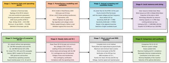
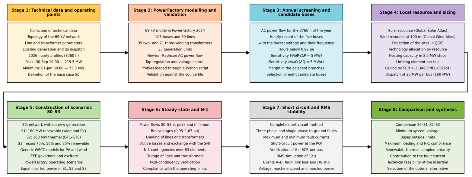
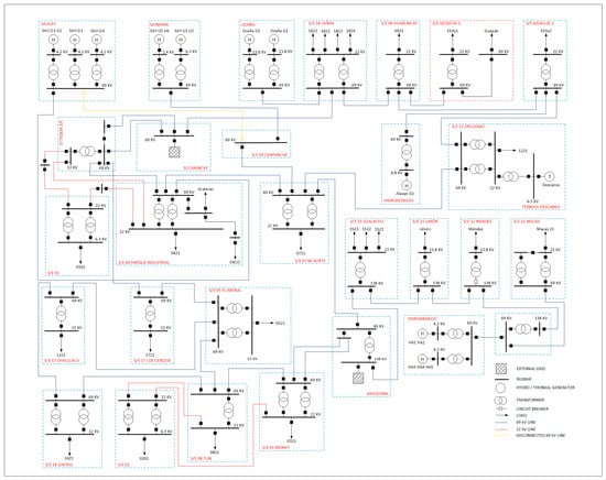
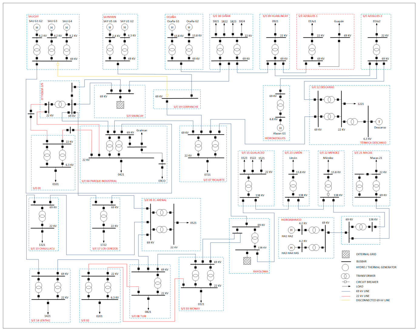
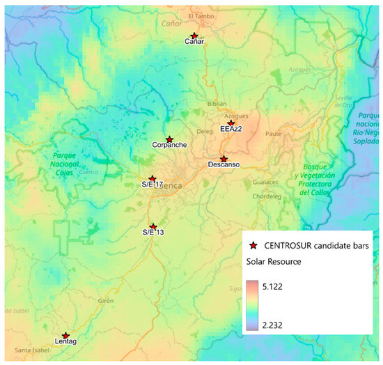
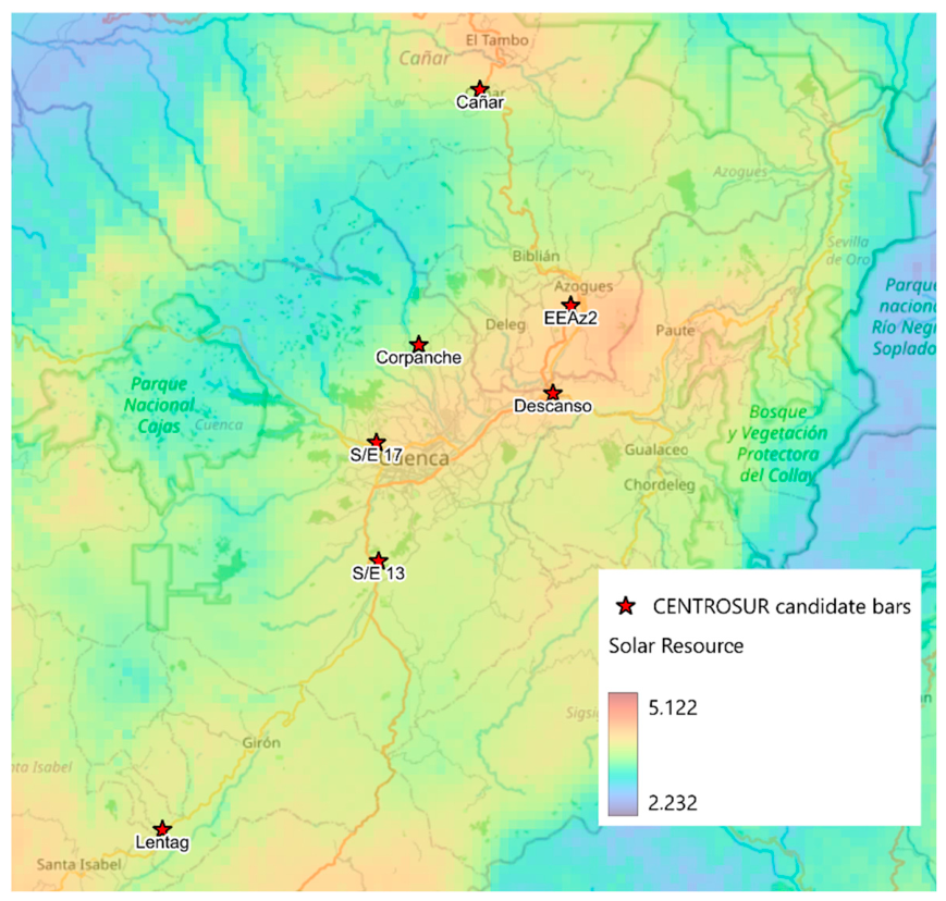
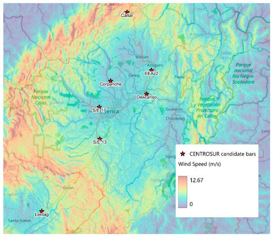
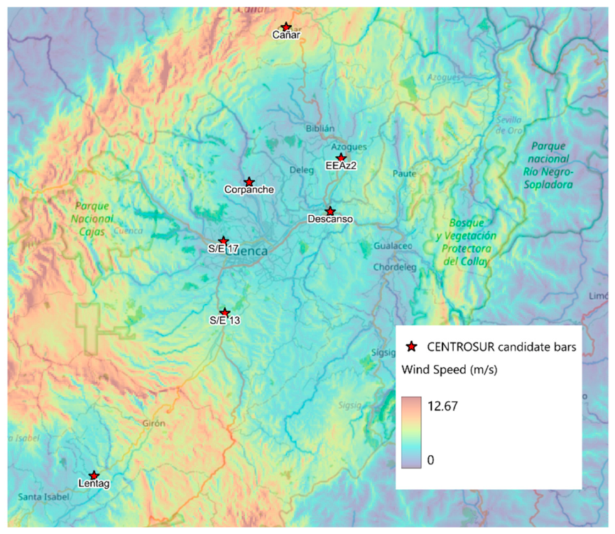
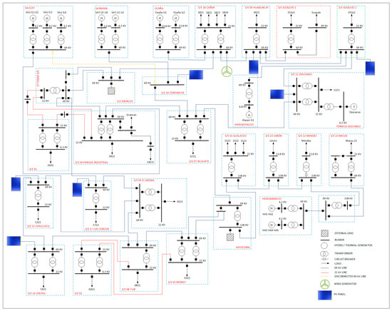
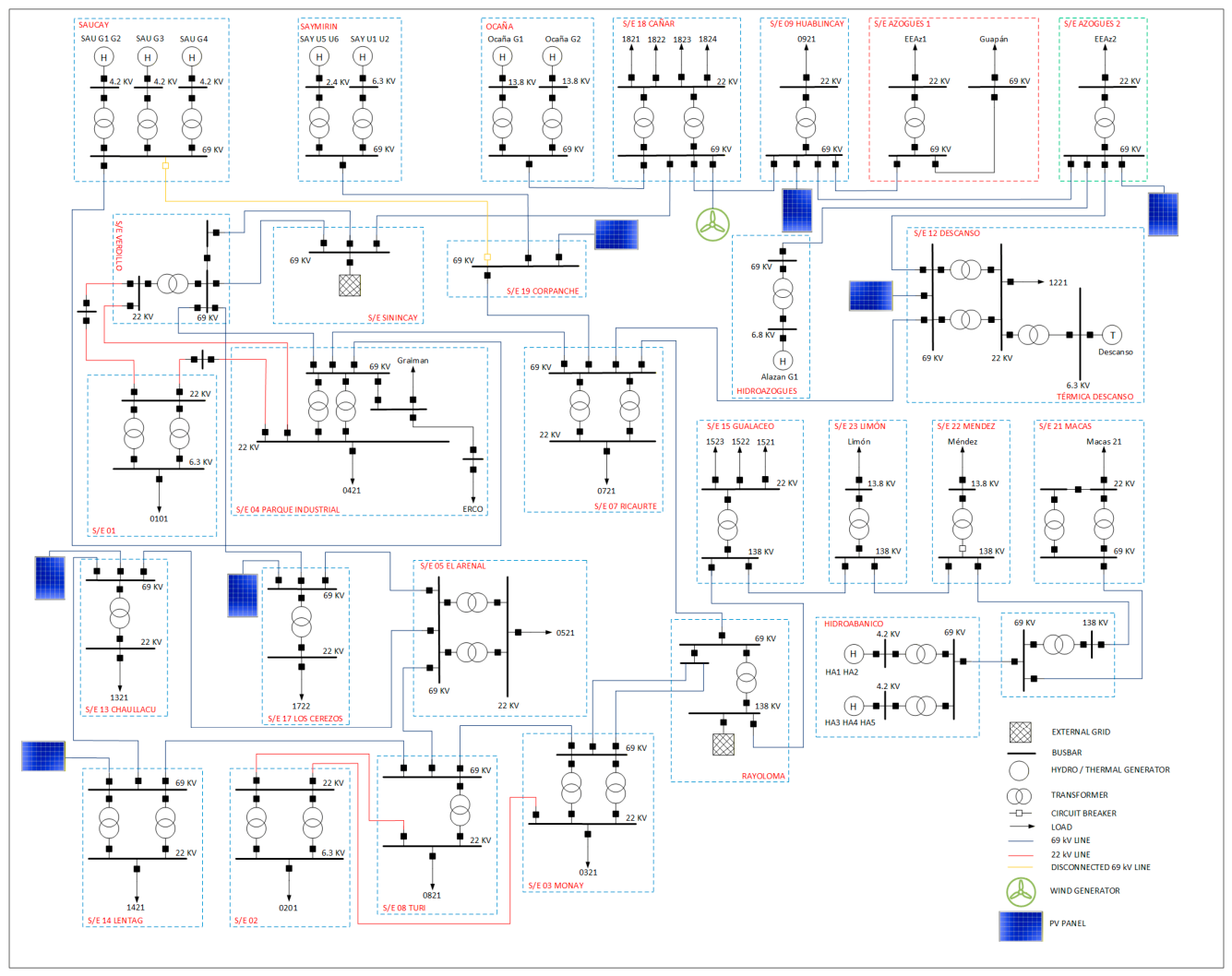
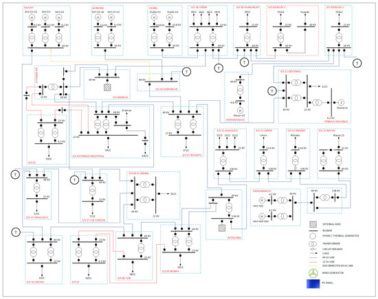
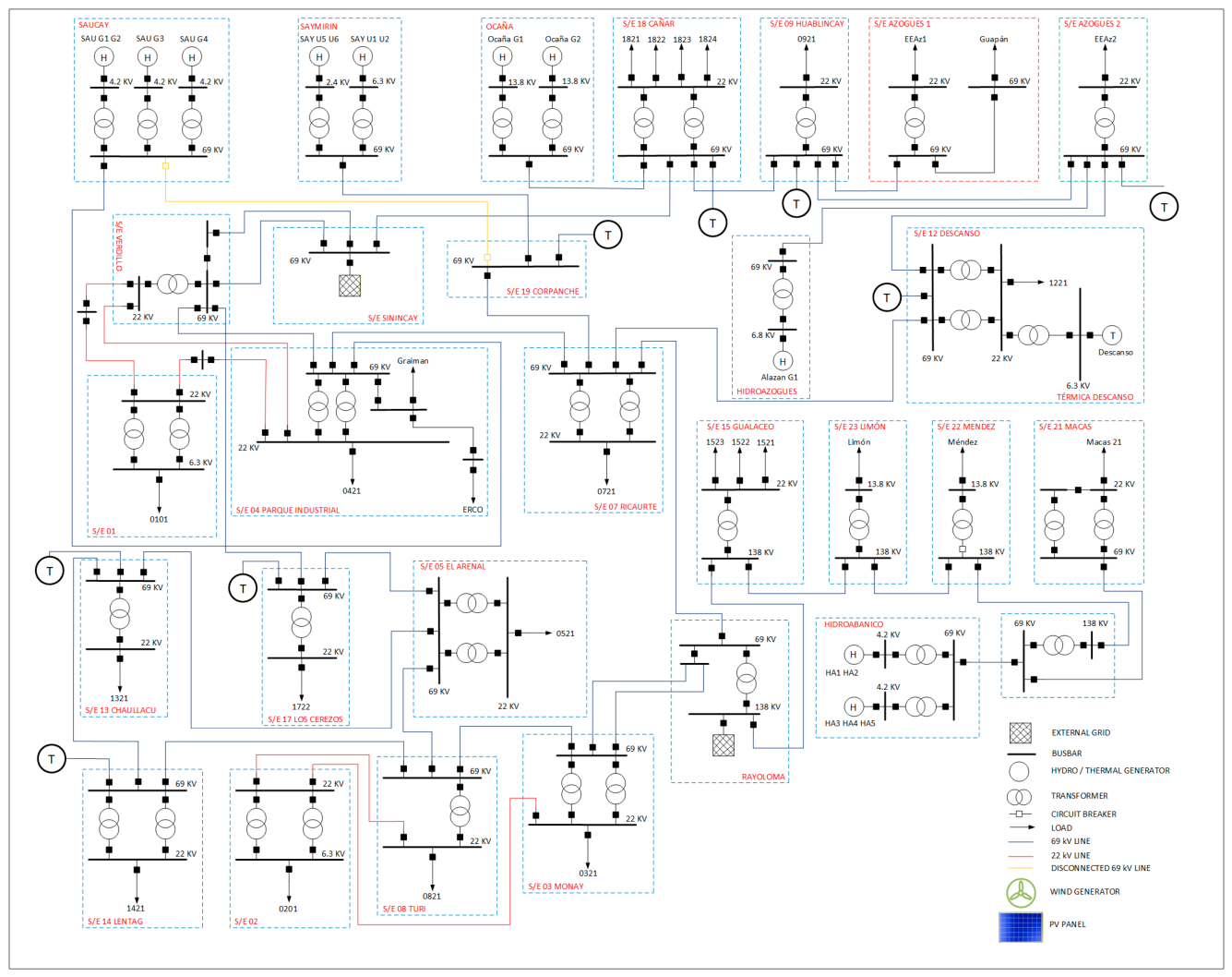
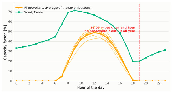
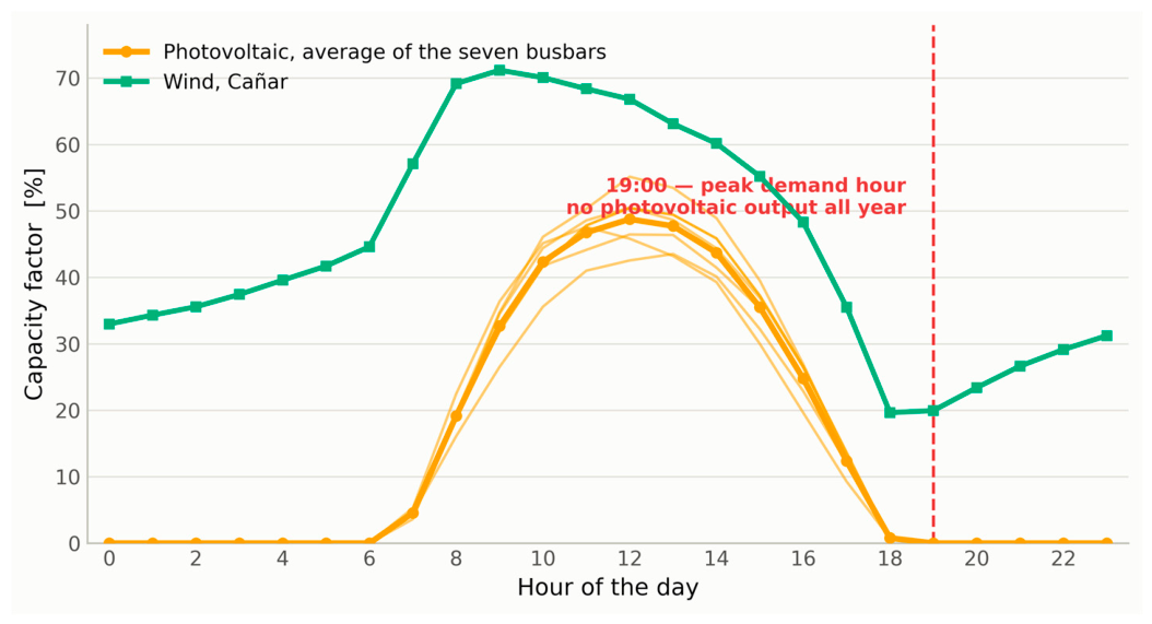
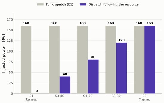
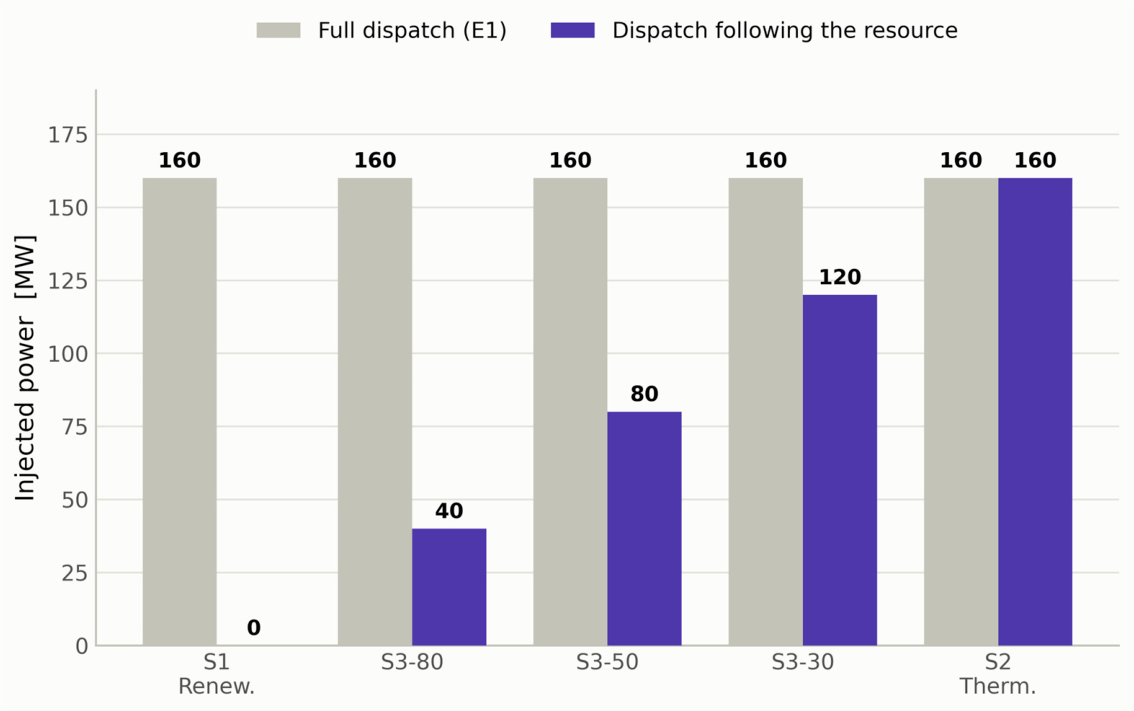
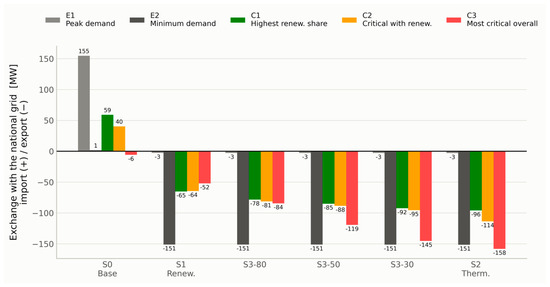
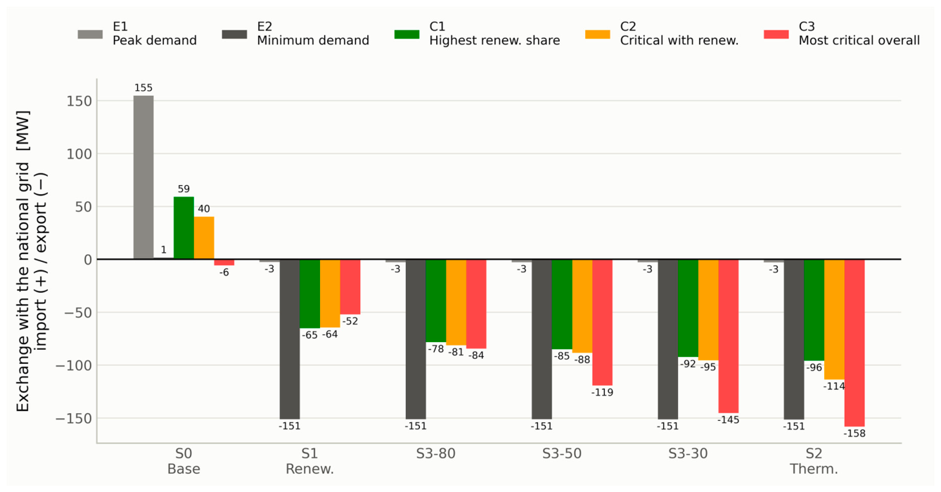
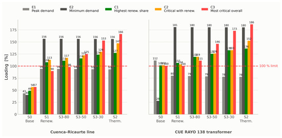
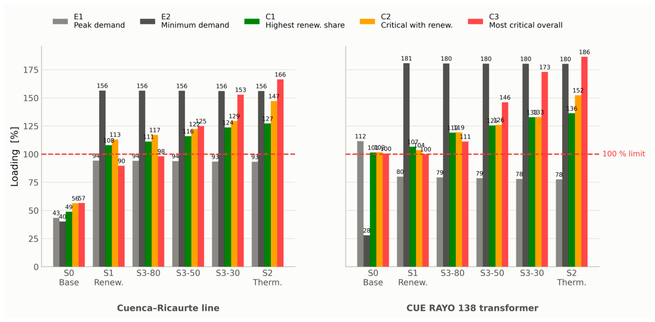
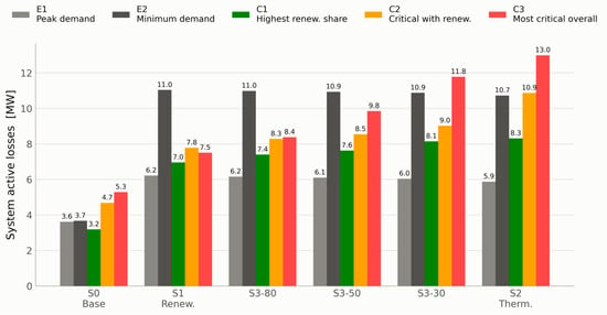
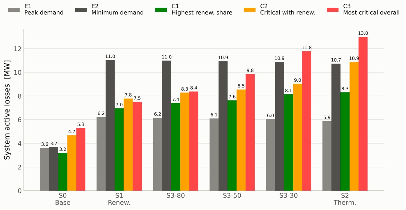
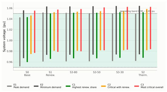
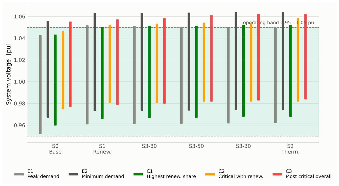
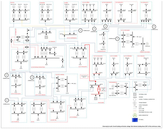
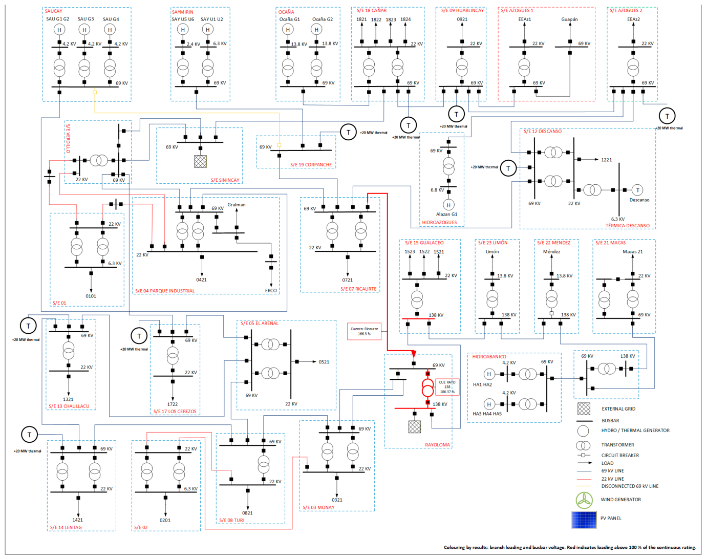
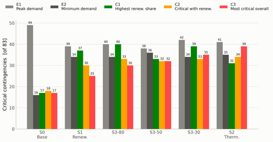
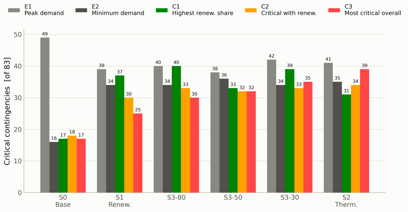
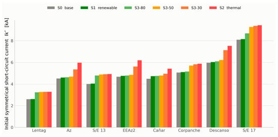
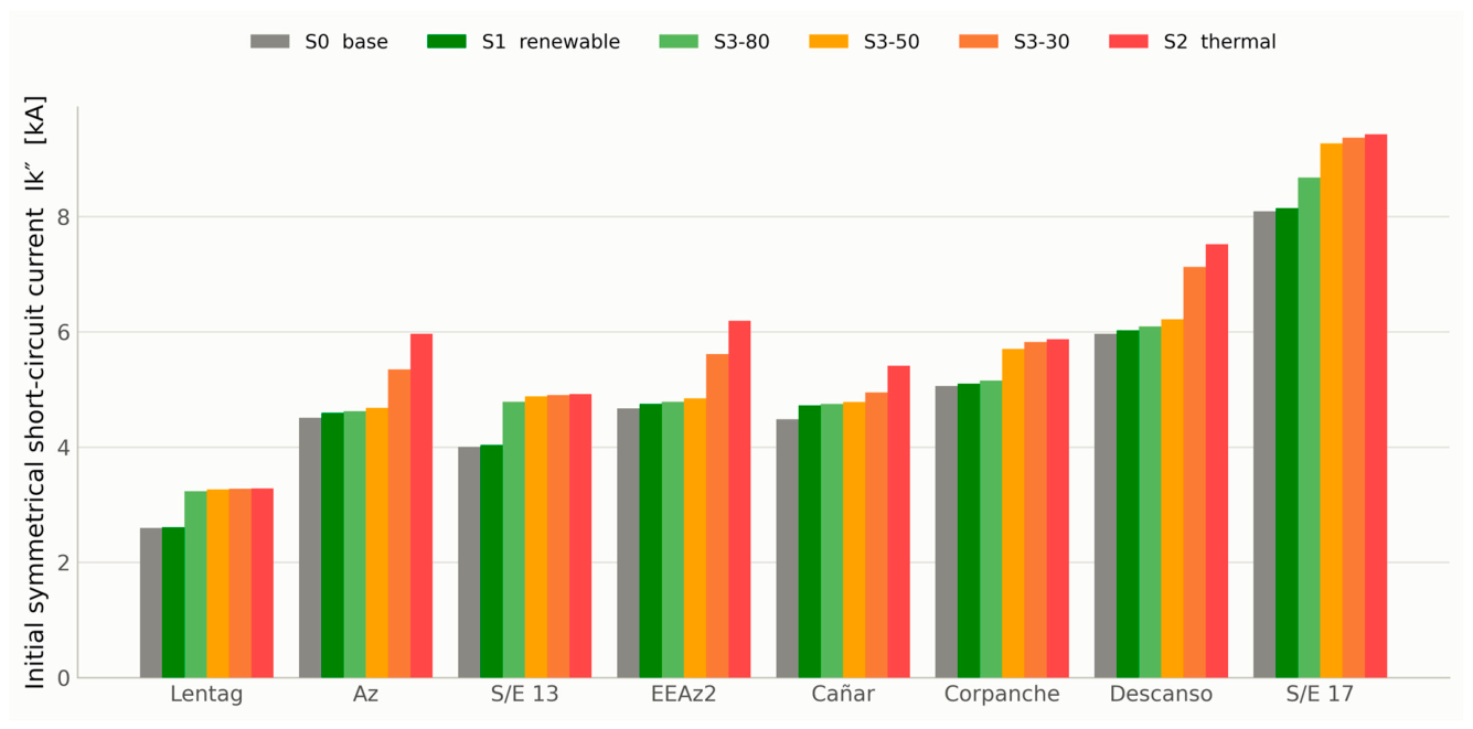
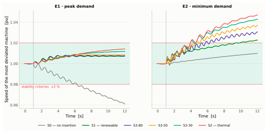
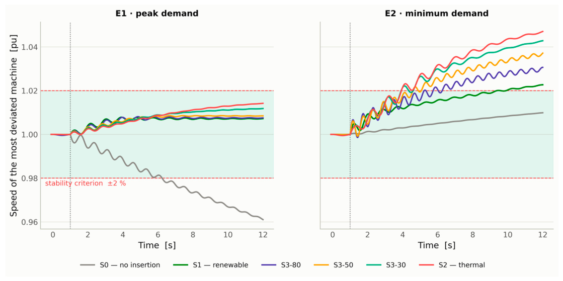
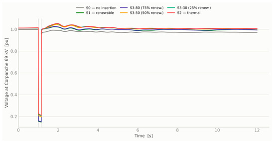
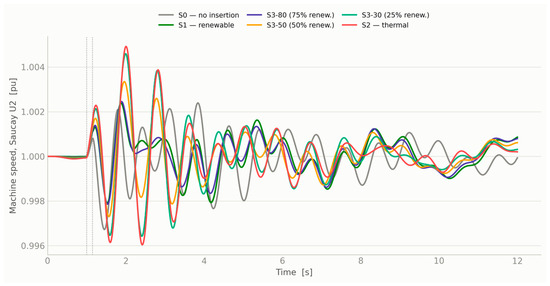
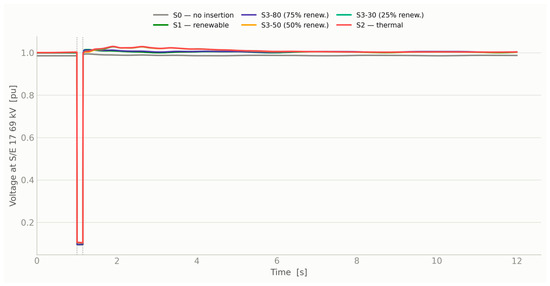
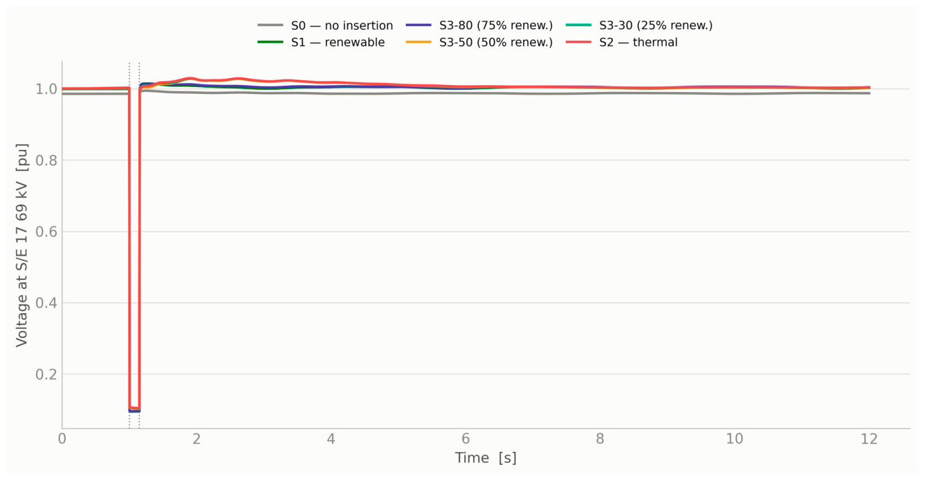
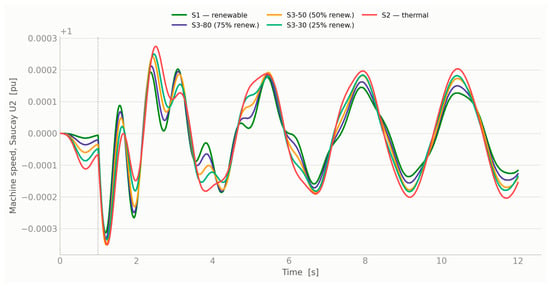
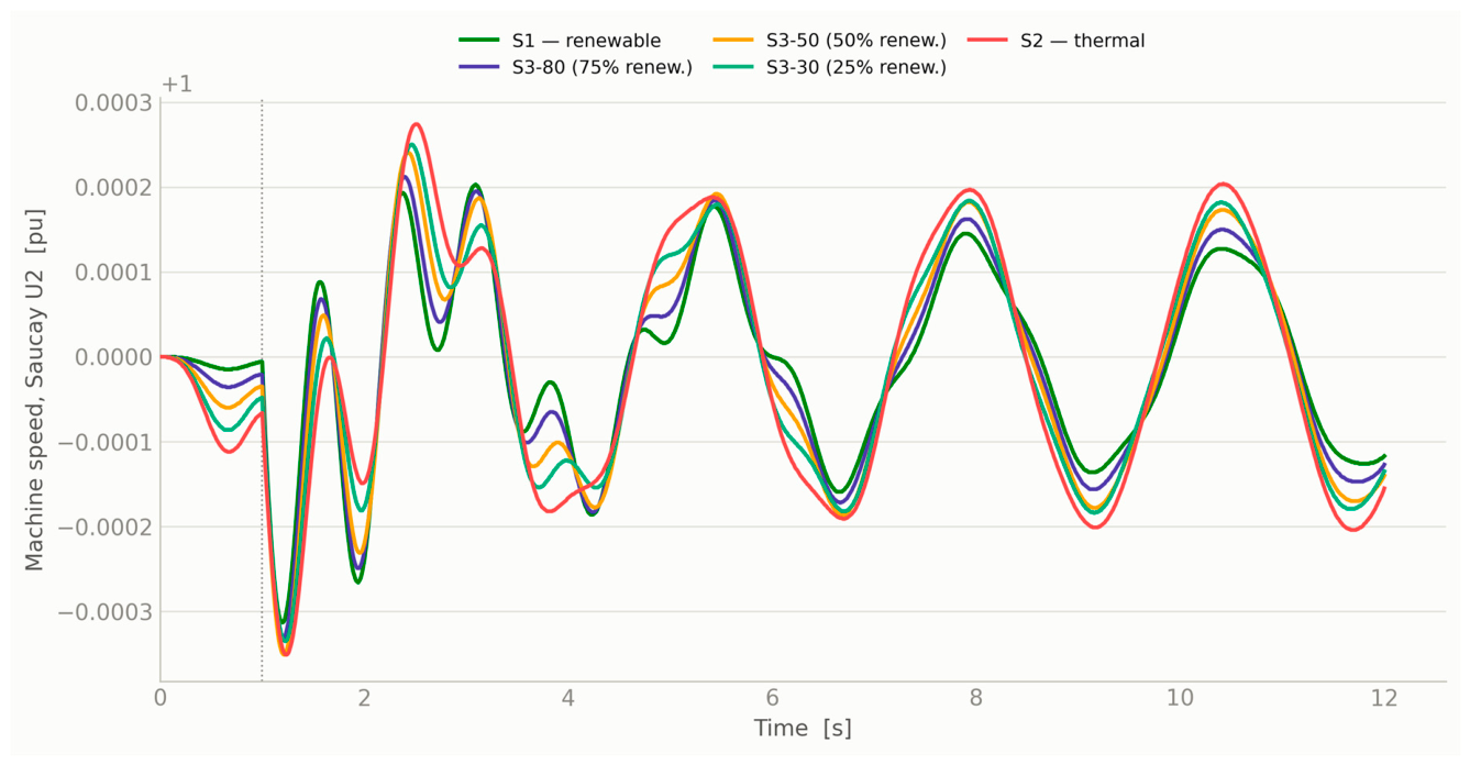
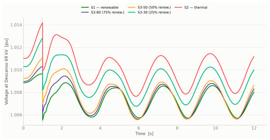
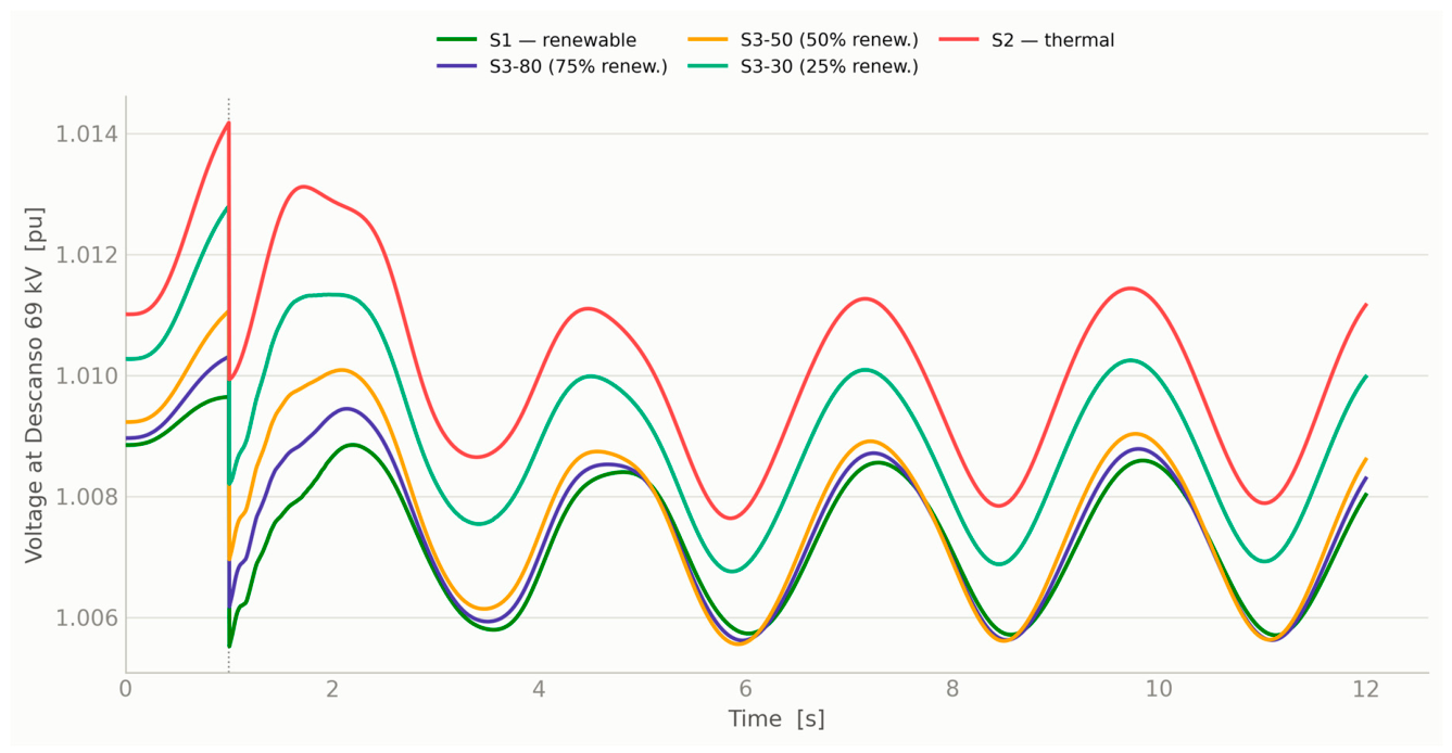

Disclaimer/Publisher’s Note: The statements, opinions and data contained in all publications are solely those of the individual author(s) and contributor(s) and not of MDPI and/or the editor(s). MDPI and/or the editor(s) disclaim responsibility for any injury to people or property resulting from any ideas, methods, instructions or products referred to in the content. |
© 2026 by the authors. Licensee MDPI, Basel, Switzerland. This article is an open access article distributed under the terms and conditions of the Creative Commons Attribution (CC BY) license.