


Abstract
Accurate faulty feeder identification is essential for the safe operation of small-current grounded distribution networks under single-phase-to-ground faults, yet existing transient-based methods often rely on preset data windows and insufficiently exploit the collective consistency of healthy feeders. This study proposes a training-free method coupling adaptive transient window selection with robust multi-feeder graph consistency analysis. Its novelty is the joint determination of which post-fault interval should be retained and which feeder deviates from the healthy feeder group. Zero-sequence current variations are obtained using one-cycle-earlier pre-fault reference waveforms, and an effective analysis window is selected within a preset maximum acquisition interval according to the cumulative transient energy ratio. The normalized current segments are then mapped to a weighted similarity graph, and a fused anomaly index based on average connection strength and median edge weight is used for feeder selection. A 110/10 kV six-feeder MATLAB/Simulink system with 180 fault cases was evaluated. With , the method achieved 98.89% accuracy with an average selected analysis-window length of 29.62 ms; accuracies under 10 and 5 dB noise were 96.17% and 91.78%, respectively. It also outperformed Haar wavelet energy and Wasserstein distance baselines in accuracy and normalized separation. These results support its effectiveness as a physically interpretable, training-free feeder identification framework.
1. Introduction
Medium-voltage distribution networks of 6–35 kV in China widely adopt neutral ungrounded operation or grounding through arc suppression coils, which are generally referred to as small-current grounded systems. When a single-phase-to-ground fault occurs, the fault current mainly flows through the line-to-ground capacitance, resulting in a relatively small current amplitude, and the system can maintain approximately balanced line voltages for a short period [1]. However, if the faulty feeder is not identified and isolated in time, the fault may further develop into phase-to-phase short circuits, multiple grounding faults, or intermittent arc grounding, and may even cause cable trench fires and large-scale outages. Therefore, fast and accurate faulty feeder identification is essential for improving protection performance and operational safety in distribution networks [2].
In ref. [3], zero-sequence current waveforms over a millisecond-scale interval from different feeders were fused, and a one-dimensional convolutional neural network (CNN) was used to automatically learn fault features. This approach reduces the subjectivity of manual feature extraction and enhances the utilization of multi-feeder correlation information. For high-impedance grounding faults in distribution networks, whose features are weak and easily confused with normal disturbances, Gao et al. [4] adopted empirical wavelet transform (EWT) to adaptively decompose differential fault energy, selected the time–frequency component with the largest permutation entropy, and constructed a permutation variance index for high-impedance fault detection. However, that method mainly focuses on fault detection and does not directly perform faulty feeder selection. High-resistance grounding faults constitute an important weak fault condition in small-current grounded distribution systems because their transient signatures may be relatively weak. In international studies on high-impedance faults (HIFs), Ghaderi et al. extracted current waveform energy and time–frequency features and validated the proposed detection method using experimental HIF data under different contact materials and operating disturbances [5]. Accordingly, the present simulation study includes fault resistances up to 1000 Ω to evaluate the proposed feeder identification method under weak fault conditions. For incipient faults, Mousavi and Butler-Purry investigated online voltage- and current-based detection in underground distribution systems using waveform-derived energy features and statistical change detection based on field measurements [6]. However, intermittent incipient faults involving repeated arc ignition and extinction are not explicitly modeled in the present work and remain an important topic for future investigation.
In ref. [7], zero-sequence currents from all feeders were superimposed into an image, and a fully convolutional network was used to segment faulty feeders, suspected faulty feeders, and healthy feeders. A fault confidence index was then constructed based on waveform similarity, improving the completeness and interpretability of the identification results.
Considering the limited availability of labeled fault samples, ref. [8] introduced generative adversarial networks (GANs) into faulty feeder identification in resonant grounding systems and improved recognition accuracy through semi-supervised learning, providing a new approach for small-sample conditions. In [9], a hybrid model consisting of patch-to-patch convolutional neural networks and feeder-to-feeder long short-term memory(LSTM) networks was proposed to fully exploit the spatial correlation and temporal dependence of zero-sequence currents.
Graph-based learning has also been introduced into power system fault diagnosis. Chanda and Soltani developed a heterogeneous graph-based multi-task learning framework that exploits network topology to jointly perform fault detection, location, classification, and estimation of fault-related quantities [10]. Such graph learning approaches demonstrate the capability of graph representations to capture structured system information, but they rely on model training. In contrast, the graph in the present study is constructed directly from pairwise transient waveform similarities among feeders and does not require labeled training data.
For the distortion of zero-sequence currents caused by distributed generation integration, ref. [11] used variational mode decomposition (VMD) to extract the overall variation trends of bus zero-sequence voltage and feeder zero-sequence currents and combined cross-correlation analysis with a harmonic energy auxiliary criterion to improve faulty feeder identification accuracy in complex distribution networks.
Reference [12] extracted transient zero-sequence current features using wavelet transform and realized faulty feeder identification through multi-scale analysis and wavelet modulus maxima, but the method is sensitive to the selected wavelet basis and decomposition level. Reference [13] used empirical wavelet transform to preprocess zero-sequence currents of each feeder and identified the faulty feeder using the Wasserstein distance coefficient between feeders, indicating the feasibility of constructing a feeder selection criterion based on waveform dissimilarity among feeders. Studies on compensated distribution networks have shown that transient-based earth fault identification can be affected by network asymmetry, cable penetration, fault resistance, and fault inception angle. Pandakov et al. further pointed out that pre-fault information can be important for improving the reliability of both steady-state and transient earth fault methods [14]. These observations indicate that transient feature extraction should account for variations in both network parameters and fault conditions. Atsever and Hocaoglu investigated faulty-feeder selection in cable-rich distribution networks with unintentional zero-sequence resonance and noted that transient zero-sequence current criteria can be sensitive to capacitive imbalance and fault resistance. They therefore proposed a transient negative sequence current criterion and evaluated it on a 151-node distribution network [15]. This study further illustrates that feeder heterogeneity and network operating conditions can influence the reliability of a fixed transient criterion. In addition to conventional feeder selection approaches, synchronized measurement technologies have also been investigated for transient event analysis and event source localization in distribution systems. Farajollahi et al. used synchronized voltage and current synchrophasors obtained from micro-phasor measurement units (micro-PMUs) to identify event sources by exploiting event-induced measurement changes and multi-location synchronized information [16]. Izadi and Mohsenian-Rad further demonstrated that synchronized time domain voltage and current waveforms can be used to locate short-duration transient events and incipient faults [17]. These studies highlight the value of exploiting transient measurement changes and coordinated multi-location information in distribution system event analysis [16,17].
For clarity, the representative methods reviewed above are comparatively summarized in Table 1 according to their principal input, training requirement, window selection strategy, main advantage, and major limitation.
Table 1.
Comparison of representative faulty feeder identification and related transient analysis methods.
The comparison is intended to clarify the methodological position of the proposed approach relative to existing transient feature, waveform distance, data-driven, and synchronized measurement-based methods. In summary, existing studies have made substantial progress in faulty feeder identification and distribution system fault analysis through transient feature extraction, time–frequency decomposition, data-driven learning, synchronized measurements, and graph-based representations. Nevertheless, several limitations remain. First, conventional transient feature methods often depend on manually selected features, decomposition parameters, or preset analysis windows, and their performance may vary with feeder parameters, fault resistance, fault inception angle, and network operating conditions. Second, data-driven and graph learning approaches can exploit complex spatial or temporal relationships, but they generally require representative labeled samples and model training. Third, fixed-length transient windows cannot readily accommodate the different transient decay rates associated with heterogeneous feeders and fault conditions. Fourth, although multi-location and multi-feeder information has been increasingly utilized, the collective waveform consistency of healthy feeders and the abnormal deviation of the faulty feeder have not been directly exploited in a training-free feeder identification framework. Therefore, a physically interpretable method that can adaptively select the effective transient interval and exploit multi-feeder relational information without relying on large-scale labeled training data is still desirable.
To address these issues, this paper proposes a training-free faulty feeder identification method that couples adaptive transient window selection with robust multi-feeder graph consistency analysis. First, after the fault inception time is supplied by an external fault-starting or protection module, the effective transient analysis window is adaptively selected within a preset maximum acquisition interval according to the cumulative transient energy ratio of the zero-sequence current variations of all feeders. This stage determines which portion of the post-fault waveform is retained for subsequent analysis. Second, the selected current segments are subjected to mean removal and unit energy normalization, and a weighted feeder similarity graph is constructed from the pairwise normalized correlation relationships. Third, a robust graph consistency anomaly index is formed by combining the average node connection strength and the median edge weight, thereby characterizing the deviation of each feeder from the healthy feeder group. The feeder with the maximum anomaly index is identified as the faulty feeder, while the gap between the largest and second-largest anomaly indices can be used for online confidence assessment.
2. Theoretical Basis of Transient Zero-Sequence Current and Multi-Feeder Consistency
2.1. Transient Zero-Sequence Current Characteristics and Zero-Sequence Network Analysis
The frequency components of transient zero-sequence currents are complex and are closely related to the phase frequency characteristics of the network. By analyzing the phase frequency characteristics of the distribution network, the corresponding phase frequency characteristics of transient zero-sequence currents can be obtained. This enables the relationship between the initial capacitive components of transient zero-sequence currents flowing out of healthy and faulty sections to be derived, and the initial capacitive frequency band of the zero-sequence network to be determined [18].
Because the grid side of the transformer connected to the load is ungrounded, the zero-sequence current path is blocked; therefore, the load can be neglected when forming the zero-sequence network [19]. The zero-sequence network under a single-phase-to-ground fault is shown in Figure 1. It should be emphasized that the frequency domain formulation in this subsection is used only to provide a physical interpretation of the consistency among healthy feeders and the abnormality of the faulty feeder. No frequency domain transformation is required in the proposed identification algorithm. The actual implementation is entirely based on sampled time domain zero-sequence current waveforms.
Figure 1.
Simplified zero-sequence equivalent network for a single-phase-to-ground fault.
The zero-sequence voltage can be regarded as the common excitation of the zero-sequence branches of all feeders. For the i-th healthy feeder, it can be simplified as , where is the equivalent zero-sequence current of the i-th feeder and is the equivalent zero-sequence admittance of the i-th feeder. In Figure 1, all six feeders except Feeder 3 are healthy feeders, and the current direction is uniformly defined from the busbar to the line. Since these healthy feeders are excited by the same bus zero-sequence voltage , their waveform directions and variation trends are generally consistent within the dominant capacitive transient frequency band. Previous studies have also established fault identification criteria based on the phase–frequency characteristics of the zero-sequence network and transient zero-sequence current relationships [18]. The red branch in the figure represents an A-phase grounding fault on Feeder 3. denotes the fault resistance at the grounding point; a smaller corresponds to a fault closer to metallic grounding, whereas a larger indicates a high-impedance grounding fault [18]. The red point denotes the A-phase grounding fault point. Because power grids in China are large in scale and have complex line structures, various random faults may occur during operation, and the neutral grounding mode is crucial for fault treatment and stable distribution network operation [11].
For healthy Feeders 1, 2, 4, 5, and 6:
For faulty Feeder 3:
where denotes the additional component caused by fault resistance, the neutral grounding branch, and distributed line parameters. All healthy feeders are excited by the common bus zero-sequence voltage and thus exhibit similar waveform trends in the dominant capacitive transient frequency band. In contrast, the zero-sequence current of the faulty feeder is affected by the fault branch and by the superposition of capacitive currents from the remaining feeders, resulting in clear differences in direction, amplitude, and waveform characteristics compared with healthy feeders. Therefore, the faulty feeder can be regarded as an abnormal feeder within the multi-feeder signal group.
It should be emphasized that the frequency domain formulation in this subsection is used only to provide a physical interpretation of the consistency among healthy feeders and the abnormality of the faulty feeder. No frequency domain transformation is required in the proposed identification algorithm. The actual implementation is entirely based on sampled time domain zero-sequence current waveforms.
2.2. Energy-Based Adaptive Transient Window
After a single-phase-to-ground fault occurs in a small-current grounded system, the zero-sequence current of each feeder generally contains both a power frequency steady-state component and a decaying oscillatory transient component, which can be expressed as
In Equation (3), and denote the steady-state component and transient component of the zero-sequence current of the i-th feeder, respectively. At the initial stage of a fault, energy exchange occurs among the line-to-ground capacitance, line inductance, and neutral grounding branch, and a pronounced high-frequency decaying oscillation appears in the zero-sequence current. As the fault process evolves, the transient component gradually decays, and the zero-sequence current eventually enters a relatively stable state. The use of adaptive filtering properties of empirical mode decomposition, together with the peak sign of low-frequency intrinsic mode functions and capacitive transient energy, indicates that transient energy and its effective frequency components can reflect faulty feeder characteristics [20].
The duration of the transient process is not fixed; rather, it is jointly affected by the fault inception angle, fault resistance at the grounding point, line length, line type, and arc suppression coil compensation status. Previous studies have shown that the effective fault waveform length differs significantly under different fault conditions. For example, in some low-resistance grounding scenarios, the transient energy is mainly concentrated in the initial fault stage and decays rapidly within several milliseconds; in high-resistance grounding or weak transient scenarios, the effective waveform may last throughout the entire preset analysis interval. Therefore, a fixed data window of identical length cannot simultaneously adapt to different fault conditions [11].
If the data window is too short, part of the slowly decaying effective transient information may be truncated, and the waveform differences among feeders cannot be fully retained. If the data window is too long, a large amount of power frequency steady-state component and background noise will be introduced, which may weaken the transient difference between faulty and healthy feeders. This issue is particularly evident in mixed overhead line and cable line networks, where the zero-sequence parameters of the two line types differ significantly and their transient oscillation frequencies and decay rates are not the same. Previous studies have found clear differences in transient decay time between pure overhead lines and cable–overhead hybrid lines, indicating the limited adaptability of a fixed window length [21].
To characterize the effective duration of the fault transient process, the zero-sequence current variation of each feeder is defined as
where is the pre-fault reference waveform at the corresponding time. The cumulative transient energy ratio of all feeders is further constructed as
where is the fault inception time and is the preset maximum analysis duration. As increases, gradually approaches a stable value. Figure 2 illustrates the cumulative energy ratio curves under different transient decay rates. When the cumulative energy reaches a given proportion, the main transient fault information can be considered to have been included, and the actual analysis window length is determined accordingly. This method enables the data window to adapt automatically to the fault transient process, retaining effective fault information while reducing the influence of subsequent steady-state components and noise, thereby providing a more suitable data basis for multi-feeder waveform consistency analysis [22].
Figure 2.
Schematic cumulative energy ratio curves under different transient decay rates.
The three curves in Figure 2 are schematic examples used only to illustrate different transient energy accumulation rates. The marked characteristic times and are illustrative values and are not obtained from specific fault cases in the simulation study. Their purpose is to demonstrate that different fault conditions may require different effective transient window lengths. The value shown in Figure 2 is used only for schematic illustration. The final energy threshold is selected according to the sensitivity analysis presented in Section 4.3.
In this study, the proposed method is activated after the fault inception time is provided by an external fault-starting or protection module. The focus of this work is faulty feeder identification after fault initiation rather than the design of the fault-starting criterion itself. In the simulation study, is directly obtained from the preset fault-switching instant, which allows for the influence of the proposed adaptive window and graph consistency identification procedures to be evaluated independently of fault-starting errors.
To reduce the influence of pre-fault load current, current transformer (CT) imbalance, and inherent zero-sequence current, the reference value at the corresponding pre-fault sampling instant is used to define the zero-sequence current variation:
The pre-fault reference is constructed using the waveform one fundamental cycle earlier. For the 50 Hz system considered in this study, , . Since the simulation output is generated using a variable step solver, the reference value at is obtained by time interpolation rather than by shifting a fixed number of samples.
Related distribution system event location studies have demonstrated that event-induced changes in synchronized voltage and current measurements can provide effective information for identifying transient disturbances and their sources. Farajollahi et al. utilized synchronized voltage and current synchrophasor measurements from micro-PMUs for event source location, whereas Izadi and Mohsenian-Rad further demonstrated the value of synchronized time domain waveform measurements for locating short-duration transient events and incipient faults. In the present study, the zero-sequence current variation is constructed by subtracting the one-cycle-earlier pre-fault reference waveform, thereby suppressing the pre-fault steady-state component before adaptive transient window determination [16,17].
The total multi-feeder transient energy at the k-th sampling point is
The cumulative energy from the fault inception time is
The total reference energy within the maximum analysis window is
Here, denotes the number of available samples whose time stamps fall within the preset maximum acquisition interval . In this study, Because the simulation uses a variable-step solver, is determined from the actual time stamps rather than from a fixed sampling frequency relationship.
The cumulative energy ratio is defined as
After fault inception, data within the fixed maximum analysis interval are first collected, and the effective transient window is then determined retrospectively according to the cumulative energy ratio. When the condition is first satisfied , the corresponding time is determined as the endpoint of the adaptive window:
In the present implementation, the adaptive transient window is selected within a preset maximum acquisition interval . Specifically, the data over are first acquired to obtain the reference cumulative energy, after which the effective transient segment satisfying the prescribed energy ratio threshold is selected for subsequent graph-consistency analysis. Therefore, represents the adaptively selected effective analysis-window length rather than an independent real-time stopping instant. Accordingly, the total elapsed decision time should be distinguished from and includes the fault detection delay, the required data-acquisition interval, and the subsequent computational time. When the cumulative energy ratio first reaches the threshold, the main transient fault information is considered to have been included. To prevent the window from becoming excessively long under weak fault conditions, the maximum analysis duration is used as an upper bound. The obtained adaptive window can avoid feature truncation caused by an overly short fixed window and suppress the steady-state components and background noise introduced by an overly long fixed window. This pre-fault reference subtraction is conceptually related to differential waveform analysis, in which event-induced waveform changes are emphasized by comparison with a pre-event reference.
2.3. Consistency and Abnormal Characteristics of Zero-Sequence Current in Multiple Feeders
For the i-th healthy feeder, the zero-sequence current within the selected transient window can be approximated as
where represents the common-state mode formed by the common bus zero-sequence voltage excitation, a_i reflects the amplitude difference caused by line length, line-to-ground capacitance, and line type, and denotes noise and local disturbances.
Since the amplitudes of different feeders may differ significantly, waveform mean removal and normalization are required before relational analysis [23]. According to the zero-sequence network current balance, the zero-sequence current of the faulty feeder can be approximated as
where denotes the additional component caused by fault resistance, the neutral branch, and distributed line parameters. Therefore, the waveform similarity between the faulty feeder and most healthy feeders is usually low, whereas healthy feeders show relatively strong consistency [24]. The correlation coefficient between the standardized zero-sequence currents of the i-th and j-th feeders is defined, and all pairwise feeder correlation coefficients form the similarity matrix as follows:
Under normal conditions, the matrix subregion corresponding to healthy feeders has high similarity, whereas the row and column corresponding to the faulty feeder usually differ significantly from the other feeders. If each feeder is regarded as a graph node and the waveform similarity between feeders is regarded as the edge weight between nodes, healthy feeders can form a tightly connected consistency group, while the faulty feeder has weak connections to this group [25]. Therefore, single-phase-to-ground faulty feeder identification can be transformed into an abnormal-node identification problem in a multi-feeder relation graph.
3. Proposed Faulty Feeder Identification Method
Overall Procedure and Multi-Feeder Graph Consistency Anomaly Index
Based on the analysis in Section 2, the effective duration of transient zero-sequence currents differs under different fault conditions. Meanwhile, healthy feeders have strong waveform consistency, whereas the faulty feeder deviates from the healthy feeder group. On this basis, this paper proposes a faulty feeder identification method combining an adaptive transient window with multi-feeder graph consistency. First, after the fault inception time is provided by the fault-starting module, post-fault data within the preset maximum acquisition interval are collected. The adaptive analysis window is then determined according to the cumulative transient energy ratio of the feeder zero-sequence current variations. Subsequently, the zero-sequence current variations within the selected window are preprocessed to construct the pairwise feeder similarity matrix and weighted relation graph. Next, the graph consistency anomaly index is calculated according to the connection relationship between each node and the remaining nodes. Finally, the faulty feeder is identified using the graph consistency anomaly index, and the separation degree of the result is evaluated using the gap between the largest and second-largest indices. The flowchart of the faulty feeder identification method is shown in Figure 3.
Figure 3.
Flowchart of proposed faulty feeder identification method.
Differences in line length, cable proportion, and line-to-ground capacitance among feeders lead to different zero-sequence current amplitude scales. Mean removal and unit-energy normalization can reduce amplitude-scale differences, allowing for subsequent analysis to mainly reflect waveform direction and variation trend [26]. The zero-sequence current sequence of the i-th feeder within the adaptive window is denoted as , and mean removal gives
Unit energy normalization is then performed, where is a small positive number used to avoid division by zero.
The similarity matrix is then constructed. The cosine similarity is denoted as . To use it as a non-negative graph edge weight, it is converted as
An adjacency matrix is formed. Each feeder is regarded as a node, and the average connection strength of the i-th node is defined as
A larger indicates stronger overall consistency between the feeder and the other feeders. The edge weights between healthy feeders are generally larger; consequently, healthy feeders have higher values, whereas the faulty feeder has weaker connections to most feeders and thus a lower .
The median edge weight between the i-th feeder and the other feeders is further defined as
The robust graph-consistency anomaly index is constructed by fusing the average connection strength and the median edge weight as
where β ∈ [0, 1] is the fusion-weight coefficient controlling the relative contributions of the average connection strength and the median edge weight. When , the anomaly index depends only on the average connection strength, whereas 0 corresponds to the median-edge-weight-only criterion. Intermediate values provide a fusion of the global connection characteristic and the robust local edge weight statistic. The influence of on feeder identification performance is further evaluated in the Sensitivity Analysis of the Fusion Weight subsection. By comparing the anomaly indices of all feeders, the faulty feeder can be selected. The faulty feeder is expected to have the largest robust anomaly index. The selection criterion is
4. Results
4.1. Simulation Model and Test Conditions
To verify the effectiveness of the proposed method, a 110/10 kV small-current grounded distribution network simulation model was established in MATLAB/Simulink R2024b, as shown in Figure 4 (The dashed boxes indicate the voltage/current measurement modules), with an L5 feeder fault illustrated as an example. The model consists of a 110 kV three-phase source, a 110/10 kV main transformer, a 10 kV bus, an arc suppression coil grounding branch, and six outgoing feeders. The rated system frequency is 50 Hz, and the neutral point on the 10 kV side is grounded through an arc suppression coil. The main transformer has a rated capacity of 31.5 MVA and a voltage ratio of 110/10 kV, with a connection. The arc suppression coil branch has a resistance of 5 Ω and an inductance of 0.55 H. Among the six feeders, L1 and L2 are overhead lines, L3 and L4 are cable lines, and L5 and L6 are overhead–cable hybrid lines, thereby introducing differences in feeder length, line type, and zero-sequence parameters.
Figure 4.
Small-current grounded system model. The dashed boxes indicate the voltage/current measurement modules.
Current measurement modules are installed at the head of each feeder to acquire three-phase currents and obtain the corresponding zero-sequence current waveforms. The feeder identification stage uses instantaneous time domain zero-sequence current waveforms rather than phasor magnitudes. The fault inception time is supplied separately by an external fault-starting or protection module; in the present simulation study, is obtained from the preset switching instant of the fault block. The electrical network is simulated in continuous mode using the variable-step ode23tb solver. The maximum solver step is set to , and the relative tolerance is . Therefore, no fixed sampling frequency is assumed in the present simulation. The proposed algorithm directly uses the actual simulation time stamps, and the pre-fault reference waveform at is obtained by time interpolation. This treatment avoids estimating an equivalent sampling frequency from nonuniform simulation samples and ensures consistency of the one-cycle pre-fault reference under variable-step simulation. The main configurations of the six feeders are summarized in Table 2.
Table 2.
Main configurations of the six feeders in the simulation model.
The positive- and zero-sequence parameters of the overhead lines are as follows: the resistances are 0.17 Ω/km and 0.23 Ω/km, the inductances are 1.21 mH/km and 5.48 mH/km, and the capacitances are 10 nF/km and 5 nF/km, respectively. For the cable lines, the corresponding positive- and zero-sequence resistances are 0.11 Ω/km and 0.28 Ω/km, the inductances are 0.52 mH/km and 1.80 mH/km, and the capacitances are 290 nF/km and 180 nF/km, respectively. These differences in line type, length, and electrical parameters result in heterogeneous transient responses among the six feeders and provide a representative test environment for evaluating the proposed multi-feeder consistency method.
4.2. Typical Case Analysis
To verify the basic faulty feeder identification process of the proposed method, an A-phase grounding fault on L3 is selected as a typical case. The fault time is set to 0.2 s, the fault location is the midpoint of the line, the fault resistance is 100 Ω, and the fault inception angle is 60 degrees. The zero-sequence current variations of all feeders after the fault are analyzed, and the results are shown in Figure 5.
Figure 5.
Changes in zero-sequence current of each feeder.
As shown in Figure 5, transient oscillations appear in the zero-sequence currents of all feeders after the fault. The waveform variation trends of L1–L2 and L4–L6 are relatively consistent, whereas the amplitude, polarity, and decay process of L3 differ significantly from those of the other feeders. This initially indicates that L3 exhibits abnormal characteristics in the multi-feeder transient response. The cumulative transient energy ratio of the zero-sequence current variations of all feeders is calculated according to Equation (11), as shown in Figure 6.
Figure 6.
Cumulative transient energy ratio curve. The horizontal dashed line denotes the preset energy-ratio threshold (), and the vertical dashed line marks the corresponding adaptive-window endpoint ().
In this section, 0.95 is used to demonstrate the calculation process of the adaptive window, while the final threshold is determined by the sensitivity analysis in Section 4.3. When the cumulative energy ratio first reaches the preset threshold of 0.95, the adaptive transient window length is obtained as . Therefore, data within 17.228 ms after the fault are used for subsequent graph consistency analysis. Within the adaptive transient window, the zero-sequence current variations of all feeders are subjected to mean removal and unit energy normalization, and the multi-feeder similarity matrix is then calculated, as shown in Figure 7.
Figure 7.
Multi-feeder similarity matrix.
The edge weights between L3 and the other feeders are significantly lower, indicating that L3 deviates from the healthy feeder group. The robust graph anomaly index of each feeder is then calculated according to Equations (19)–(22), as shown in Figure 8.
Figure 8.
Robust graph anomaly indicators.
The anomaly index of L3 is significantly larger than those of the other feeders; therefore, L3 is identified as the faulty feeder. This result is consistent with the simulation setting and verifies the effectiveness of the proposed method in a typical single-phase-to-ground fault scenario.
To evaluate the influence of the adaptive transient window on faulty feeder identification, fixed data windows of different lengths are compared with the adaptive window method. For the fixed window method, zero-sequence current data of 5 ms, 10 ms, 20 ms, 40 ms, 60 ms, and 80 ms after the fault are respectively extracted to calculate the graph-consistency anomaly index. For the adaptive window method, the effective analysis window is automatically determined according to the cumulative transient energy ratio defined in Equation (11). Except for the data window length, the signal preprocessing, similarity matrix construction, and anomaly index calculation procedures remain unchanged. Test samples are constructed by varying the faulty feeder, fault location, fault resistance, and fault inception angle. For each fault case, different fixed windows and the adaptive window are used for feeder identification, and the identification accuracy and anomaly index separation are recorded. Let be the number of correctly identified cases and be the total number of test cases; the identification accuracy is defined as
To further evaluate the distinction between the faulty feeder and healthy feeders, the anomaly index separation is defined as
where is the robust anomaly index of the actual faulty feeder, and denotes the largest anomaly index among all healthy feeders. When , the anomaly index of the faulty feeder is higher than those of all healthy feeders; a larger D indicates clearer separation between the faulty and normal feeders. For the k-th case, if the identification result is correct and , the case is counted as a low-confidence case. In this study, . A low-confidence case means that the faulty feeder is correctly identified but the gap between its anomaly index and that of the closest healthy feeder is small, making the result more sensitive to noise or parameter disturbances. Misclassified cases correspond to and are not counted as low-confidences; instead, they are reflected by the identification accuracy and minimum separation. The separation index D defined above uses the known true faulty feeder and is therefore employed only for offline performance evaluation in the simulation study. For online confidence assessment, the gap between the largest and second-largest anomaly indices can be calculated without requiring prior knowledge of the actual faulty feeder. It should be emphasized that is used only for post hoc confidence analysis of the simulation results and does not participate in faulty feeder identification. The faulty feeder is determined solely by the maximum graph consistency anomaly index. Therefore, changing does not change the predicted feeder or the identification accuracy.
4.3. Effectiveness Analysis of the Adaptive Transient Window
To verify the influence of transient analysis window selection on faulty feeder identification, fixed and adaptive data windows are compared. The fixed window method extracts zero-sequence current data within 5 ms, 10 ms, 20 ms, 40 ms, 60 ms, and 80 ms after fault inception, respectively. The adaptive window method automatically determines the analysis window according to the cumulative transient energy ratio of zero-sequence current variations of all feeders. To further analyze the influence of the energy threshold on adaptive window performance, five energy thresholds, namely 0.90, 0.95, 0.97, 0.98, and 0.99, are considered in the sensitivity analysis. Except for the data window selection strategy, all experiments use the same fault inception time, zero-sequence current preprocessing, similarity matrix construction, and graph consistency anomaly index calculation procedures.
L1, L3, and L5 are selected as faulty feeders, and fault locations are set at 20%,50%, and 80% of the line length. Fault resistances are set to 0 Ω, 100 Ω, 500 Ω, and 1000 Ω, and fault inception angles are set to 0 degrees, 15 degrees, 30 degrees, 60 degrees, and 90 degrees, forming 180 fault cases in total. For each case, faulty feeder identification is performed using different data windows, and the identification accuracy, average window length, average separation, minimum separation, and number of low-confidence cases are calculated. The experimental results are shown in Table 3.
Table 3.
Comparison of faulty feeder identification performance under different data windows.
Table 3 shows that the identification results vary significantly under different fixed window lengths, indicating that the effective duration of the fault transient is not constant. Figure 9 shows the change in identification accuracy under different fixed window lengths.
Figure 9.
Identification accuracy under different fixed window lengths.
The 5 ms fixed window achieves an identification accuracy of only 94.44%, lower than most other window lengths, indicating that an excessively short data window may truncate effective transient information and prevent sufficient extraction of waveform differences between the faulty and healthy feeders. The 20 ms fixed window achieves an accuracy of 97.78%, but the number of low-confidence cases reaches 15, suggesting that although some cases are correctly identified under this window length, the anomaly index separation margin between the faulty feeder and the closest healthy feeder is small, and the identification stability is insufficient.
When the fixed window length increases to 40 ms, 60 ms, and 80 ms, all three windows achieve an identification accuracy of 98.89%, indicating that longer analysis windows can cover the main transient process in most cases. However, fixed window methods require a unified window length to be preset manually, and the optimal value is related to the fault location, fault resistance, fault inception angle, and other factors; therefore, they still depend on engineering experience. Although the 10 ms fixed window also achieves 98.89% accuracy and has the highest average separation and the smallest number of low-confidence cases, it is essentially an empirical window selection strategy and cannot guarantee optimality in other systems or broader operating conditions.
The identification performance is not expected to vary monotonically with the fixed window length. Changing the window length modifies the relative waveform similarity structure among all feeders rather than simply increasing the amount of useful information. For some fault cases, an intermediate window may include weaker post-transient components that reduce the contrast between the faulty feeder and the healthy feeder group, resulting in the observed fluctuation in identification accuracy.
To reduce reliance on empirical fixed window lengths, the influence of the energy threshold in the adaptive window is further analyzed, as shown in Figure 10.
Figure 10.
Influence of the adaptive window energy threshold.
As shown in Figure 10, when the energy threshold increases from 0.90 to 0.99, the average adaptive window length increases from 22.80 ms to 32.97 ms, indicating that a higher energy threshold retains more transient information. Meanwhile, the identification accuracy of the adaptive window increases from 97.78% to 98.89%, and the number of low-confidence cases decreases from 14 to 2. As the energy threshold increases, the average selected window length increases because a larger proportion of the transient energy is retained. The identification accuracy generally improves and then remains stable, whereas the average separation varies non-monotonically with the threshold. Therefore, the threshold is selected by jointly considering identification accuracy, low-confidence cases, and window length rather than by maximizing the separation index alone.
When the threshold is 0.97, 0.98, or 0.99, the adaptive window achieves an identification accuracy of 98.89%. For , the average window length is 29.62 ms, the number of low-confidence cases is 2, and the average separation is 0.2180. Although produces similar performances, the average window length further increases to 32.97 ms. Considering the identification accuracy, the number of low-confidence cases, and the average selected window length, is adopted as a representative operating value in this study. It should be noted that is not obtained through data-driven training or optimization. The results for , show similar identification accuracy, indicating that the proposed method maintains stable performance over a relatively broad threshold range rather than relying on a uniquely optimized value. Because the sensitivity analysis and the final evaluation are conducted using the same simulation case set, should be regarded as a representative operating value for the present system rather than a universally optimized threshold. Independent validation across different network configurations and operating conditions will be considered in future work.
Compared with the 40 ms, 60 ms, and 80 ms fixed windows, the selected adaptive window maintains the same 98.89% identification accuracy and the same number of low-confidence cases while reducing the average window length by approximately 10.38 ms, 30.38 ms, and 50.38 ms, respectively. This indicates that the proposed adaptive window can reduce unnecessary data length while maintaining identification performance.
In summary, fixed window methods can achieve high accuracy under some window lengths, but their performance is sensitive to the selected window and still relies on engineering experience. The cumulative transient energy-based adaptive window proposed in this paper can automatically adjust the analysis interval according to different fault conditions and balance window length and identification stability by tuning the energy threshold. The finally selected adaptive_eta098 strategy achieves 98.89% identification accuracy with two low-confidence cases over 180 fault cases, and its average window length is only 29.62 ms. These results show that the proposed method reduces the dependence on fixed window experience while providing stable and compact data for subsequent multi-feeder graph consistency analysis.
4.4. Noise Robustness Analysis
To further verify the stability of the proposed method under noise interference, this section compares the window strategies that achieved 98.89% accuracy under the noise-free condition in Section 4.3, including fixed windows of 10 ms, 40 ms, 60 ms, and 80 ms, as well as the adaptive window with . Gaussian white noise is added separately to the zero-sequence currents of the six feeders, and the signal-to-noise ratio (SNR) is set to 30 dB, 20 dB, 10 dB, and 5 dB. At each SNR level, random noise is repeated 10 times. The reported noise performance metrics are averaged over the ten independent noise realizations. In contrast, the noise-free simulations are deterministic for a given fault condition, so repeated execution of the same case does not introduce additional statistical variability. For the same fault case, SNR level, and repetition, all window strategies use exactly the same noisy waveform to ensure a fair comparison. The SNR is defined as follows:
The identification results of different window strategies under different noise levels are listed in Table 4, and the corresponding trends are shown in Figure 11, including (a) accuracy, (b) average separation index, and (c) low-confidence cases.
Table 4.
Performance comparison of fixed and adaptive windows under different noise levels.
Figure 11.
Identification performance of different window strategies under different noise levels: (a) identification accuracy; (b) average separation; (c) low-confidence cases.
As shown in Table 4 and Figure 11a, under light noise, i.e., SNR = 30 dB, all window strategies maintain an identification accuracy of 98.89%, indicating that the proposed graph consistency anomaly index is generally stable under weak noise interference. At this stage, the accuracy differences among different window strategies are not obvious; however, the average separation of the adaptive window reaches 0.3016, which is significantly higher than those of the 10 ms, 40 ms, 60 ms, and 80 ms fixed windows. This indicates that the anomaly index difference between the faulty and healthy feeders is more pronounced under the adaptive window. It is worth noting that the average selected adaptive window length increases as the SNR decreases, from 39.07 ms at 30 dB to 87.31 ms at 5 dB. This increase should not be interpreted as an extension of the physical fault transient itself. Since the adaptive window criterion is constructed from the cumulative squared zero-sequence current variations, additive noise also contributes to the accumulated energy. Under low-SNR conditions, the total energy is therefore distributed over a longer interval, and a longer selected window is required for the cumulative energy ratio to reach the prescribed threshold . Thus, the increase in reflects the combined influence of useful transient information and noise contamination rather than a longer physical transient duration.
This behavior reveals a robustness–window length tradeoff: under severe noise, the adaptive strategy retains a longer signal segment to preserve sufficient discriminative information, at the cost of an increased selected analysis window length. Therefore, the adaptive strategy should not be interpreted as guaranteeing the shortest analysis window under all conditions; rather, it adaptively balances information retention and robustness as the signal quality changes. When the SNR decreases to 20 dB, the accuracy of fixed window methods begins to decline. The accuracies of the 10 ms, 40 ms, 60 ms, and 80 ms fixed windows are 95.72%, 96.56%, 96.39%, and 95.94%, respectively, whereas the adaptive window with still maintains 98.89% accuracy. Meanwhile, the average separation of the adaptive window is 0.2382, which is higher than those of all fixed window strategies, and the number of low-confidence cases is also significantly smaller. This result indicates that under moderate noise, the adaptive window can improve the discrimination margin between the faulty and healthy feeders by retaining sufficient effective transient information. The 87.31 ms average selected window at 5 dB also indicates that the adaptive strategy does not necessarily produce the shortest analysis window under all operating conditions. Under severe noise, retaining a longer segment provides more waveform information for the subsequent multi-feeder similarity analysis, but at the cost of increased data window length. Therefore, the adaptive strategy should be interpreted as providing a robustness–window length tradeoff rather than as universally minimizing the analysis window duration.
When the SNR further decreases to 10 dB and 5 dB, the noise interference becomes stronger, and the identification performance of all methods decreases. Nevertheless, the adaptive window still exhibits stronger noise robustness than the fixed window methods. At SNR =10 dB, the accuracy of the fixed window methods is approximately 86–87%, whereas the adaptive window accuracy reaches 96.17%. At SNR = 5 dB, the fixed window accuracy is approximately 82–83%, whereas the adaptive window still achieves 91.78%. This shows that under strong noise, the adaptive window can effectively alleviate the performance degradation caused by insufficient transient information or an increased noise proportion in fixed windows.
The average separation trends in Figure 11b show that as the SNR decreases, the average separation of all methods gradually decreases, indicating that noise weakens the anomaly index difference between the faulty and healthy feeders. However, the average separation of the adaptive window remains higher than those of all fixed window strategies at all noise levels. For example, at SNR = 10 dB, the adaptive window has an average separation of 0.1574, whereas all fixed window methods have values below 0.10. At SNR = 5 dB, the adaptive window still achieves an average separation of 0.1101, higher than those of all fixed window methods. This result indicates that the adaptive window maintains a better discrimination margin under noise interference. Although the adaptive strategy maintains higher identification accuracy under severe noise, the increasing number of low-confidence cases indicates that the separation between the faulty feeder and the closest healthy feeder becomes less pronounced as the SNR decreases. Therefore, the robustness improvement should be interpreted jointly in terms of identification accuracy, separation index, and low-confidence statistics, rather than accuracy alone.
Overall, the adaptive window with achieves the highest or tied-highest identification accuracy under all noise levels, and its average separation is consistently higher than those of the fixed window strategies. Under medium and low SNR conditions, the adaptive window shows a more pronounced advantage over fixed windows. In particular, at SNR=10 dB and 5 dB, the adaptive window accuracy is approximately 9–10 percentage points higher than that of the fixed window methods, demonstrating that the proposed adaptive transient window can effectively improve the robustness of graph consistency-based feeder identification under noise interference.
4.5. Ablation Study
To further analyze the contributions of each key module in the proposed method to faulty feeder identification performance, an ablation study is designed. The ablated components mainly include two parts: the transient window selection strategy and the composition of the graph consistency anomaly index. The transient window strategies include a fixed 40 ms window and the adaptive transient window with . The anomaly-index components include the node average connection strength, the median edge weight, and their fusion.
Five ablation variants are compared, as shown in Table 5. Variant A uses the fixed 40 ms window and the average connection strength index. Variant B uses the fixed 40 ms window and the median edge weight index. Variant C uses the fixed 40 ms window and the fused index. Variant D uses the adaptive window with and the average connection strength index. The proposed method is the complete method, which uses the adaptive window with and the fused graph consistency anomaly index. All variants are tested under the same 180 fault cases, with the faulty feeders, fault locations, fault resistances, and fault inception angles kept consistent with the previous sections. The performance comparison of different ablation variants is presented in Table 5 and Figure 12.
Table 5.
Numerical performance metrics of different ablation variants.
Figure 12.
Graphical comparison of different ablation variants.
As shown in Table 5 and Figure 12a, all five ablation variants correctly identify 178 of the 180 fault cases, yielding an accuracy of 98.89%. This indicates that, under the noise-free condition, the graph consistency identification framework based on multi-feeder similarity has strong overall faulty feeder identification capability. Since the accuracy values are the same for all variants, the contributions of different modules should be further analyzed using the average separation, number of low-confidence cases, and average window length.
Comparing Variant A with Variant C under the fixed 40 ms window, using only the average connection strength yields an average separation of 0.1982 and four low-confidence cases. After the median edge weight is further fused, the average separation increases to 0.2187 and the number of low-confidence cases decreases to two. This result shows that the median edge weight can complement the average connection strength in characterizing local abnormal edge weights. The fusion of the two indicators reduces low-margin correct identifications in some boundary cases and thereby improves the discrimination stability of the graph consistency anomaly index.
Comparing Variant C with the proposed method, both use the fused graph consistency index and achieve an identification accuracy of 98.89%, with two low-confidence cases. Their average separations are 0.2187 and 0.2180, respectively, which are very close. However, Variant C uses a fixed 40 ms window, whereas the proposed method uses the adaptive window with reducing the average window length from 40.00 ms to 29.62 ms, a reduction of approximately 25.95%. This indicates that the adaptive transient window can reduce reliance on manual fixed window selection and reduce redundant data length without substantially degrading identification accuracy or discrimination stability.
It should be noted that Variant B has the highest average separation, 0.2378, indicating that the median edge weight alone also provides strong discrimination under noise-free conditions. However, Variant B still depends on the fixed 40 ms data window and characterizes feeder abnormality only from the perspective of median edge weight. In contrast, the proposed method determines the effective transient interval using the adaptive window and fuses the average connection strength with the median edge weight, thereby balancing high identification accuracy, a small number of low-confidence cases, window length adaptivity, and index comprehensiveness.
In summary, the ablation study demonstrates that both the average connection strength and the median edge weight can reflect the abnormal characteristics of the faulty feeder relative to the healthy feeder group. Compared with the mean-only index, the fused index increases the average separation and reduces the number of low-confidence cases. The adaptive transient window shortens the average analysis window without sacrificing identification accuracy. Therefore, the proposed method achieves a good balance among identification accuracy, discrimination stability, and window length adaptivity. Since the two graph statistics exhibit different characteristics in terms of average and worst-case separation, their relative fusion weight is further examined through a sensitivity analysis.
Sensitivity Analysis of the Fusion Weight
To further investigate whether the proposed graph consistency anomaly index is sensitive to the relative weighting of the average connection strength and median edge weight, a sensitivity analysis of the fusion coefficient was conducted. Five representative values, , were considered. The adaptive window threshold was fixed at = 0.98, and all other algorithm settings and the same 180 fault cases were kept unchanged. Here, represents the median-edge-weight-only criterion, whereas represents the average-connection-strength-only criterion, as shown in Table 6.
Table 6.
Sensitivity of faulty feeder identification performance to the fusion weight .
The identification accuracy remains 98.89% for , while only a slight decrease to 98.33% is observed when . This indicates that the proposed graph consistency criterion maintains stable feeder identification performance over a broad range of fusion weights and is not strongly dependent on a specific value of . The selected adaptive window length is identical for all tested weights because is applied only after the adaptive transient window has been determined.
The average separation decreases from 0.2370 to 0.1976 as increases from 0 to 1, whereas the minimum separation improves from −0.0945 to −0.0642. This tradeoff indicates that the median edge weight provides stronger average discrimination, while the average connection strength contributes complementary information in difficult boundary cases. Considering the stable identification accuracy over the intermediate weight range and avoiding an additional empirical preference toward either statistic, is retained as an equal-weight setting in the proposed method.
4.6. Comparison with Typical Transient Feature-Based Methods
To further verify the superiority of the proposed method over typical transient feature-based faulty feeder identification methods, Haar wavelet energy and Wasserstein distance methods are selected for comparison. The Haar wavelet energy method identifies the faulty feeder by extracting the high-frequency transient energy of zero-sequence currents at the initial fault stage, whereas the Wasserstein distance method identifies the faulty feeder by measuring the distributional differences among transient wave forms of different feeders. The proposed method uses the adaptive transient window with = 0.98 and the fused graph consistency anomaly index determined previously.
For a fair comparison, all three methods use the same fault inception time and the same zero-sequence current data. The Haar wavelet energy method and Wasserstein distance method use the 40 ms fixed analysis window that performed well in Section 4.3, while the proposed method uses the adaptive analysis window with . The test cases are still the 180 single-phase-to-ground fault cases described above, including different faulty feeders, fault locations, fault resistances, and fault inception angles. Since the original decision indices of different methods have different dimensions, the feeder scores obtained by each method are normalized using min–max normalization to compare the discrimination margins uniformly:
where is the original decision score of the i-th feeder, is the normalized feeder score, and is a small positive number used to avoid division by zero. The unified separation index is defined as
where f denotes the actual faulty feeder. If the score of the actual faulty feeder is higher than those of all healthy feeders; if . The identification results of different methods are shown in Table 7.
Table 7.
Performance comparison of different faulty feeder identification methods.
As shown in Table 7, the Haar wavelet energy method correctly identifies 82 out of 180 fault cases, with an accuracy of 45.56%. This method identifies the faulty feeder only according to the magnitude of transient high-frequency energy. However, in single-phase-to-ground faults of small-current grounded systems, healthy feeders may also exhibit significant transient components due to zero-sequence network coupling. Therefore, a simple maximum energy criterion is easily disturbed by the transient responses of non-faulty feeders, leading to low identification accuracy.
The Wasserstein distance method correctly identifies 138 cases, achieving an accuracy of 76.67%, which is significantly higher than that of the Haar wavelet energy method. This indicates that, compared with a single energy feature, a distance criterion based on waveform distribution differences can better reflect transient response differences between faulty and healthy feeders. However, this method judges only from the perspective of pairwise waveform distribution distances and does not further exploit the overall consistency relationship among multiple feeders. Therefore, misidentifications still occur in some high-resistance grounding or weak transient cases.
In contrast, the proposed method correctly identifies 178 out of 180 cases, achieving an accuracy of 98.89%, which is significantly higher than those of the Haar wavelet energy and Wasserstein distance methods. Meanwhile, the proposed method has an average normalized separation index of 0.6999, higher than −0.1491 for the Haar wavelet energy method and 0.4128 for the Wasserstein distance method. This indicates that the proposed method distinguishes faulty and healthy feeders with a larger discrimination margin. In terms of low-confidence cases, the proposed method has two cases, which is slightly higher than the one case obtained by the Wasserstein distance method but substantially fewer than the eight cases of the Haar wavelet energy method, indicating relatively stable discrimination in boundary cases.
In terms of average window length, both the Haar wavelet energy method and the Wasserstein distance method use a fixed 40 ms window, whereas the proposed method has an average adaptive window length of 29.62 ms. In other words, the proposed method achieves the highest identification accuracy and the largest average separation with a shorter average data window. This indicates that the adaptive transient window can extract an effective analysis interval according to the post-fault transient energy accumulation process, avoiding possible transient information truncation or redundant steady-state data introduced by fixed windows.
The average computation times of the Haar wavelet energy and Wasserstein distance methods are 1.05 ms and 2.12 ms, respectively, whereas that of the proposed method is 6.95 ms. It should be emphasized that the reported 6.95 ms represents only the algorithmic computation time after the required waveform data have been acquired; it does not represent the total elapsed decision time from fault inception. In the present implementation, the adaptive window selection requires the data within the preset maximum acquisition interval to be available before the effective analysis segment is determined. Therefore, the total elapsed decision time consists of the fault-starting delay, the preset data-acquisition interval, and the subsequent computational processing time. Although the proposed method introduces higher computational overhead than the two comparison methods, the graph analysis stage itself remains at the millisecond level. Overall, the Haar wavelet energy method relies only on transient energy features and is easily affected by healthy feeder transient responses. The Wasserstein distance method can characterize waveform distribution differences but does not sufficiently exploit overall multi-feeder correlation features. The proposed method extracts effective fault transient information through the adaptive transient window and constructs an anomaly index based on multi-feeder graph consistency, enabling more stable faulty feeder identification. Therefore, the proposed method exhibits better overall performance in terms of identification accuracy, discrimination margin, and number of low-confidence cases.
4.7. Practical Applicability and Limitations
The proposed feeder identification method requires synchronized time domain zero-sequence current waveforms from the outgoing feeder heads and a fault inception signal supplied by an external fault starting or protection module. No labeled training data or frequency domain decomposition is required. Therefore, the proposed algorithm can in principle be implemented as a post-fault feeder identification function in a substation protection or monitoring device.
The six-feeder simulation system includes overhead, cable, and overhead–cable hybrid feeders, introducing differences in line length, capacitance, and transient response. Mean removal and unit energy normalization reduce the influence of amplitude-scale differences among heterogeneous feeders. Nevertheless, the present system cannot represent all practical feeder configurations, and extreme parameter differences may weaken the consistency among healthy feeders.
The present study treats each outgoing feeder as one graph node and aims to identify the faulty parent feeder. Detailed localization of faults on laterals or branched sections is outside the current scope. More complex branched distribution topologies, larger feeder numbers, and distributed generation penetration should therefore be investigated in future work. In addition, the present validation is limited to a resonant-grounded system using an arc suppression coil. Other neutral grounding modes may alter the zero-sequence current relationships among feeders; therefore, the present parameter settings and consistency assumptions should not be transferred directly to other grounding conditions without independent validation.
The current noise study adopts additive Gaussian white noise (AWGN) as a controlled measurement noise model. Practical feeder current measurements may additionally contain CT ratio and phase errors, CT saturation, harmonics, impulsive disturbances, non-Gaussian noise, synchronization errors, and communication uncertainties. Therefore, the present noise results should be regarded as an initial robustness assessment rather than a complete representation of field measurement conditions. In addition, the pairwise graph construction requires feeder similarities, and its computational burden increases approximately quadratically with the number of feeders. Further validation using field recordings and larger-scale substations is needed before practical deployment. A full module-wise ablation under multiple noise and measurement nonideality conditions will also be considered to further quantify the interaction between adaptive window selection and graph anomaly index construction.
5. Conclusions
This paper addresses the problems of insufficient adaptability of fixed data windows, inadequate utilization of multi-feeder correlation features, and the dependence of deep-learning methods on large numbers of training samples in single-phase-to-ground faulty feeder identification for small-current grounded systems. A faulty feeder identification method based on an adaptive transient window and robust multi-feeder graph consistency is proposed. Through theoretical analysis and MATLAB/Simulink simulation verification, the following conclusions are obtained.
- (1)
- The adaptive transient window based on the cumulative transient energy ratio can automatically determine the analysis interval according to the decay characteristics of transient processes under different fault conditions. The results of 180 fault cases show that when the energy threshold is = 0.98, the adaptive window achieves an identification accuracy of 98.89% with an average window length of 29.62 ms. Compared with the 40 ms, 60 ms, and 80 ms fixed windows, the proposed method shortens the average analysis window while maintaining the same identification accuracy, reducing reliance on manual fixed window selection.
- (2)
- The graph consistency anomaly index based on multi-feeder similarity can effectively characterize the abnormal features of the faulty feeder relative to the healthy feeder group. The ablation study shows that after fusing the average connection strength and the median edge weight, the number of low-confidence cases is smaller than that of the mean-only index, indicating that the fused index improves discrimination stability in boundary cases. Meanwhile, the adaptive window reduces the average window length from 40.00 ms to 29.62 ms while maintaining nearly unchanged identification accuracy and number of low-confidence cases, validating the effectiveness of the adaptive window module.
- (3)
- The noise robustness experiments show that as the SNR decreases, the identification accuracy and average separation of all window strategies are affected to different degrees. Compared with fixed window methods, the adaptive window with = 0.98 maintains higher identification accuracy and larger average separation under 20 dB, 10 dB, and 5 dB noise conditions. In particular, at SNR = 10 dB and 5 dB, the adaptive window accuracies reach 96.17% and 91.78%, respectively, significantly higher than those of the fixed window strategies, demonstrating improved robustness relative to the tested fixed window strategies under the considered AWGN conditions.
- (4)
- Compared with the Haar wavelet energy and Wasserstein distance methods, the proposed method correctly identifies 178 out of 180 fault cases, achieving an accuracy of 98.89% and an average normalized separation index of 0.6999. The results show that a single transient energy feature is easily affected by healthy feeder transient responses, while waveform distance methods can describe differences among feeders but do not sufficiently exploit overall multi-feeder consistency. By extracting effective transient information through the adaptive transient window and constructing an anomaly index based on multi-feeder graph consistency, the proposed method identifies faulty feeders more reliably.
Although the proposed method shows promising simulation performance, the current study is limited to a six-feeder simulation system and controlled Gaussian noise conditions. Future work will focus on field fault recordings, CT nonidealities, complex branched topologies, distributed generation, and larger-scale networks.
Author Contributions
Conceptualization, J.Y. and H.Z.; methodology, J.Y.; software, J.Y.; validation, J.Y. and Z.J.; formal analysis, J.Y.; investigation, J.Y.; writing—original draft preparation, J.Y.; writing—review and editing, H.Z. and Z.J.; supervision, H.Z. All authors have read and agreed to the published version of the manuscript.
Funding
This study is funded by Inner Mongolia Agricultural University, with the project name being “Theoretical Research on Economic Dispatch of West Inner Mongolia Power Grid with High-Proportion Wind Power Cluster Integration” and the project number being RZ2100002054. The Article Processing Charge (APC) is also funded by the same project.
Data Availability Statement
The data presented in this study are available from the corresponding author upon reasonable request.
Acknowledgments
The authors would like to thank the College of Mechanical and Electrical Engineering, Inner Mongolia Agricultural University, for its support during this study.
Conflicts of Interest
The authors declare no conflicts of interest.
References
- Qing, T. Accurate grounding line selection technology for small-current grounded systems and its application. Lamps Light. 2025, 49, 112–115. [Google Scholar]
- Liu, J.; Zhang, X.H.; Zhang, X.Q.; Zhang, Z.H.; Xu, B.Y.; Xu, Y.; Li, R.G. Single-phase grounding fault handling in small-current grounded systems for preventing cable trench fires. Power Syst. Prot. Control 2023, 51, 21–29. [Google Scholar]
- Gao, J.; Guo, M.; Chen, D. Fault line detection using waveform fusion and one-dimensional convolutional neural network in resonant grounding distribution systems. CSEE J. Power Energy Syst. 2021, 7, 250–260. [Google Scholar] [CrossRef] [Scilit]
- Gao, J.; Wang, X.; Wang, X.; Yang, A.; Yuan, H.; Wei, X. A high-impedance fault detection method for distribution systems based on empirical wavelet transform and differential faulty energy. IEEE Trans. Smart Grid 2022, 13, 900–912. [Google Scholar] [CrossRef] [Scilit]
- Ghaderi, A.; Mohammadpour, H.A.; Ginn, H.L., III; Shin, Y.-J. High-Impedance Fault Detection in the Distribution Network Using the Time-Frequency-Based Algorithm. IEEE Trans. Power Deliv. 2015, 30, 1260–1268. [Google Scholar] [CrossRef] [Scilit]
- Mousavi, M.J.; Butler-Purry, K.L. Detecting Incipient Faults via Numerical Modeling and Statistical Change Detection. IEEE Trans. Power Deliv. 2010, 25, 1275–1283. [Google Scholar] [CrossRef] [Scilit]
- Yu, X.; Gu, J.; Zhang, X.; Mao, J. GAN-based semi-supervised learning method for identification of the faulty feeder in resonant grounding distribution networks. Int. J. Electr. Power Energy Syst. 2023, 144, 108535. [Google Scholar] [CrossRef] [Scilit]
- Yuan, J.; Jiao, Z. Faulty feeder detection for single phase-to-ground faults in distribution networks based on patch-to-patch CNN and feeder-to-feeder LSTM. Int. J. Electr. Power Energy Syst. 2023, 147, 108909. [Google Scholar] [CrossRef] [Scilit]
- Yuan, J.; Hu, Y.; Liang, Y.; Jiao, Z. Faulty feeder detection for single line-to-ground fault in distribution networks with DGs based on correlation analysis and harmonics energy. IEEE Trans. Power Deliv. 2023, 38, 1020–1029. [Google Scholar] [CrossRef] [Scilit]
- Chanda, D.; Soltani, N.Y. A Heterogeneous Graph-Based Multi-Task Learning for Fault Event Diagnosis in Smart Grid. IEEE Trans. Power Syst. 2025, 40, 1427–1438. [Google Scholar] [CrossRef] [Scilit]
- Gao, J.; Yang, S.; Xu, S.; Du, Z.; Xu, Y. Research on single-phase grounding fault of power system based on new small current grounding system. J. Phys. Conf. Ser. 2024, 2781, 012019. [Google Scholar] [CrossRef] [Scilit]
- Wang, C.Y.; Li, Z.Y. Analysis of single-phase fault feeder selection in small-current grounded systems based on wavelet theory. Electron. Technol. 2025, 54, 224–225. [Google Scholar]
- Zhou, M.; Li, M.; Shan, H. Distribution Network Faulty Feeder Detection Method Based on Empirical Wavelet Transform and Wasserstein Distance Coefficient. J. Electr. Eng. Technol. 2025, 20, 3755–3766. [Google Scholar] [CrossRef] [Scilit]
- Pandakov, K.; Høidalen, H.K.; Marvik, J.I. Misoperation Analysis of Steady-State and Transient Methods on Earth Fault Locating in Compensated Distribution Networks. Sustain. Energy Grids Netw. 2018, 15, 34–42. [Google Scholar] [CrossRef] [Scilit]
- Atsever, M.B.; Hocaoglu, M.H. A Faulty Feeder Selection Method for Distribution Network with Unintentional Resonance in Zero Sequence Circuit. Electr. Power Syst. Res. 2023, 223, 109587. [Google Scholar] [CrossRef] [Scilit]
- Farajollahi, M.; Shahsavari, A.; Stewart, E.M.; Mohsenian-Rad, H. Locating the Source of Events in Power Distribution Systems Using Micro-PMU Data. IEEE Trans. Power Syst. 2018, 33, 6343–6354. [Google Scholar] [CrossRef] [Scilit]
- Izadi, M.; Mohsenian-Rad, H. Synchronous Waveform Measurements to Locate Transient Events and Incipient Faults in Power Distribution Networks. IEEE Trans. Smart Grid 2021, 12, 4295–4307. [Google Scholar] [CrossRef] [Scilit]
- Wang, X.W.; Shi, F.; Zhang, H.X.; Xue, J.R.; Zhen, Z.H.; Xie, W.; Ling, P.; Liu, J. Single-phase grounding fault section location method for small-current grounded systems based on transient energy. Power Syst. Technol. 2019, 43, 818–825. [Google Scholar] [CrossRef]
- Wang, P.; Chen, B.; Zhou, H.; Tian, C.; Sun, B. Fault location in resonant grounded network by adaptive control of neutral-to-earth complex impedance. IEEE Trans. Power Deliv. 2018, 33, 689–698. [Google Scholar] [CrossRef] [Scilit]
- Wang, L.; Luo, W.; Weng, L.; Hu, Y.; Li, B. Single Line-to-ground Fault Location and Information Modeling Based on the Interaction between Intelligent Distribution Equipment. J. Electr. Eng. Technol. 2018, 13, 1807–1813. [Google Scholar] [CrossRef]
- Chu, T.X.; Zhang, W.H.; Qu, K.; Zhang, S.; Xiao, X.; Tan, Y. Disturbance characteristics of grounding incipient faults in small-current grounded systems. Power Syst. Prot. Control 2021, 49, 52–61. [Google Scholar] [CrossRef]
- Yuan, J.W.; Jiao, Z.B. Faulty feeder identification method for small-current grounded systems based on full-waveform recognition of zero-sequence signals. Power Syst. Technol. 2024, 48, 839–853. [Google Scholar] [CrossRef]
- Cheng, W.A.; Xu, M.; Gao, J.F. Spatial-domain image generation and fusion method for single-phase-to-ground faulty feeder selection in small-current grounded systems. Electr. Power Autom. Equip. 2021, 41, 97–103. [Google Scholar] [CrossRef]
- Feng, G.; Guan, T.L.; Wang, L.; Xue, Y.; Yu, X.; Xu, B. Grounding fault feeder selection in small-current grounded systems using the linearity relationship between current and voltage derivatives. Power Syst. Technol. 2021, 45, 302–311. [Google Scholar] [CrossRef]
- Wan, G.J.; Xu, X. Research on single-phase grounding detection method in small-current grounding systems based on image recognition. Front. Energy Res. 2024, 12, 1473472. [Google Scholar] [CrossRef] [Scilit]
- Zhang, H.; Zhang, D.H.; Liu, N.Y.; Wu, K.Z.; Shi, Z. Single-phase-to-ground faulty feeder identification method for small-current grounded systems based on improved VMD and ConvNeXt. High Volt. Eng. 2025, 51, 730–741. [Google Scholar] [CrossRef]
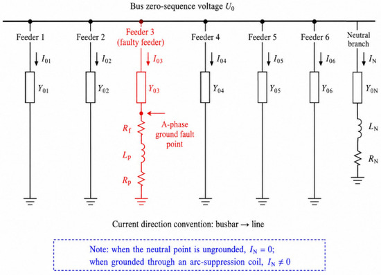
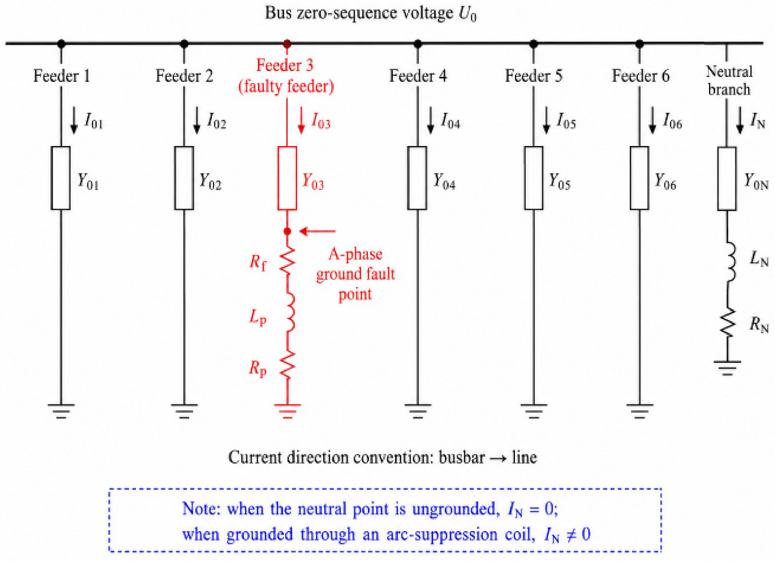
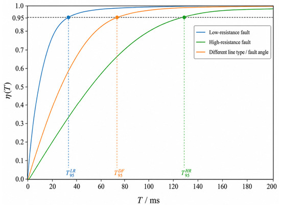
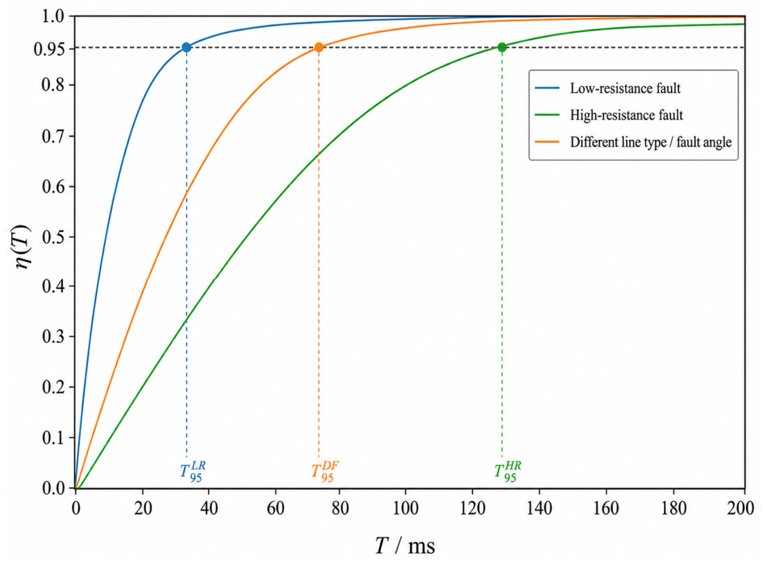
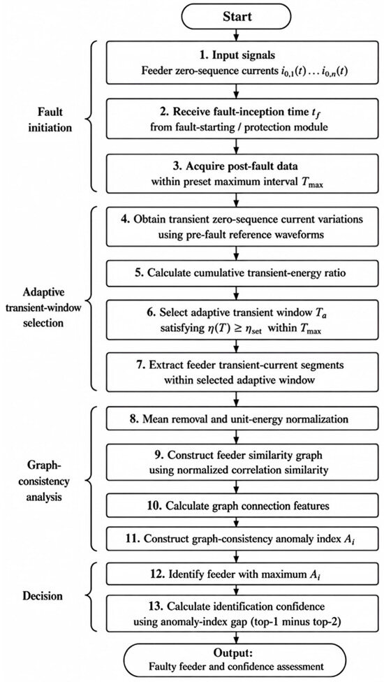
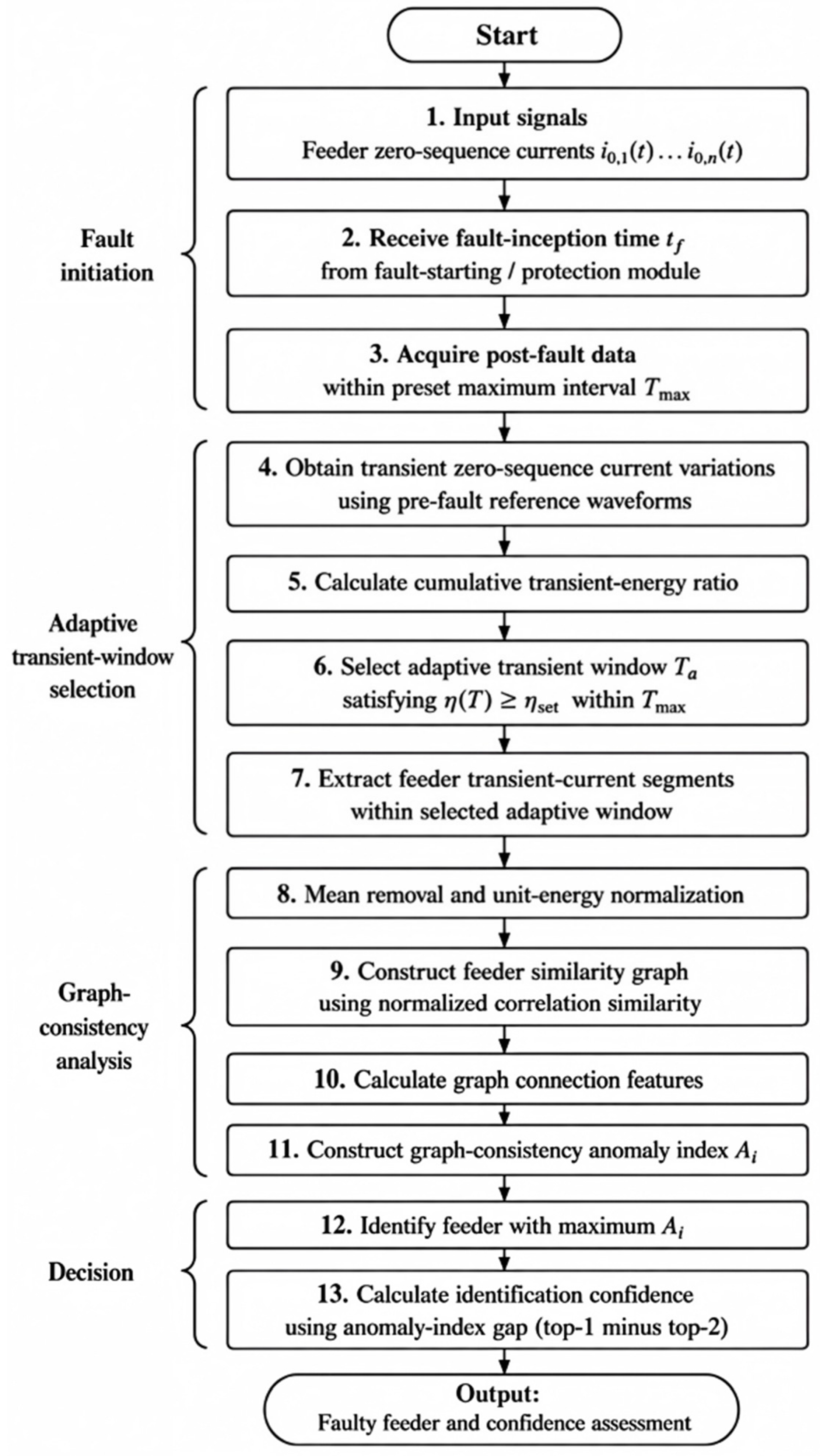
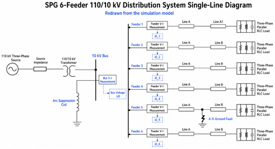
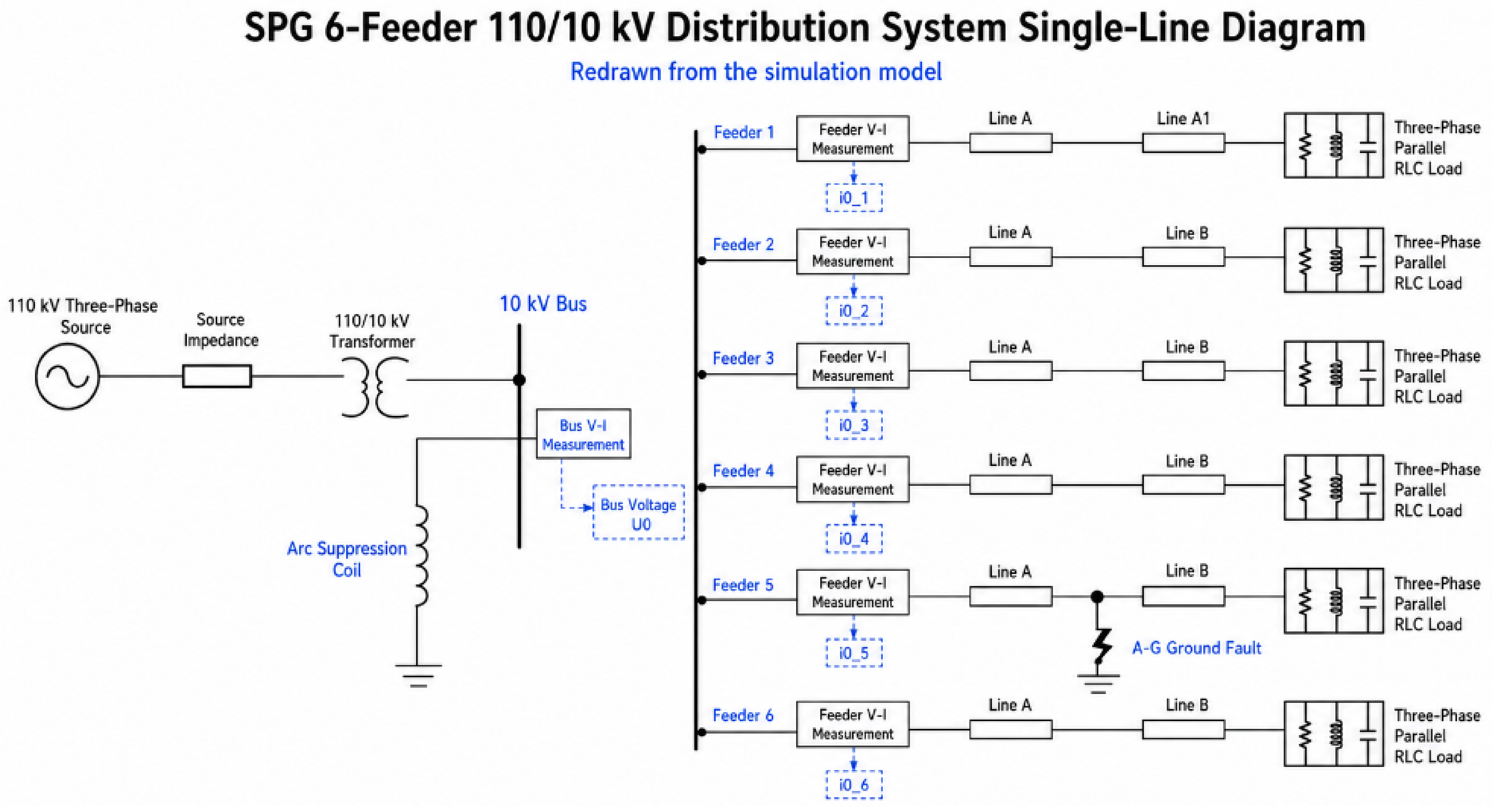
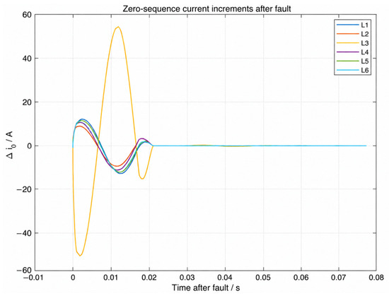
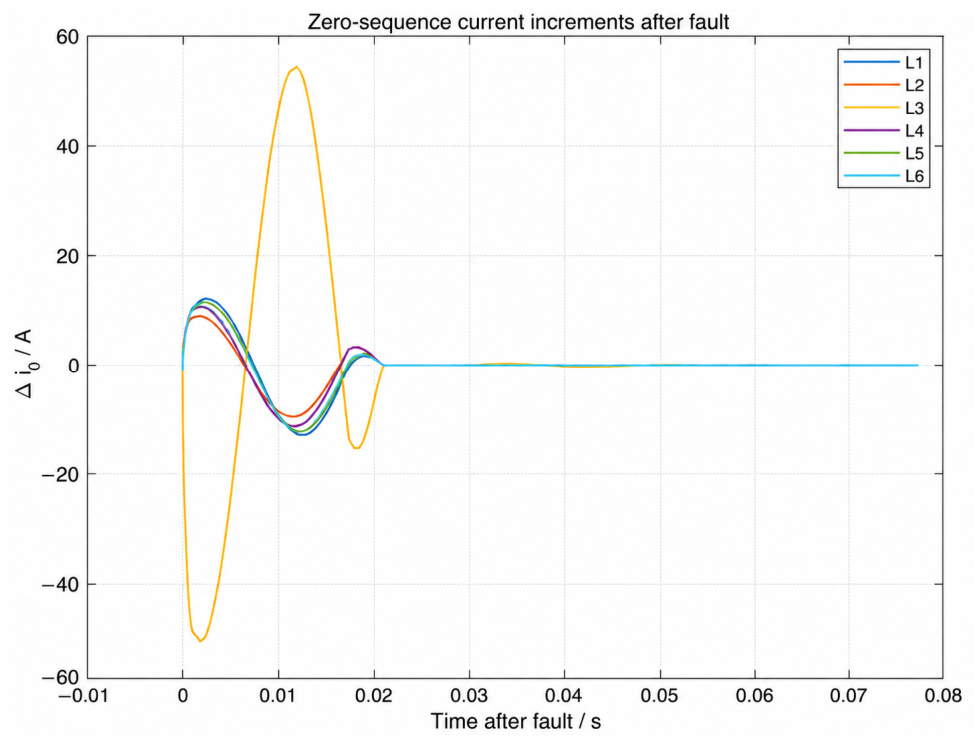
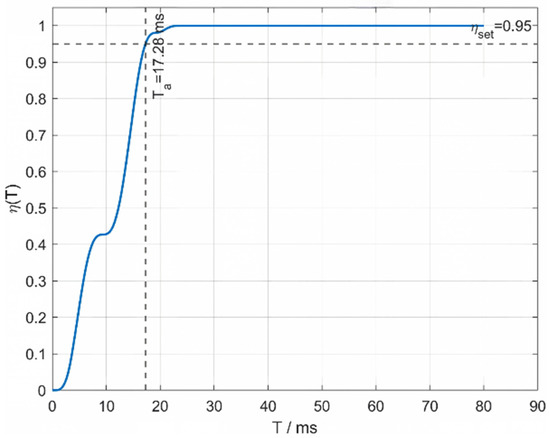
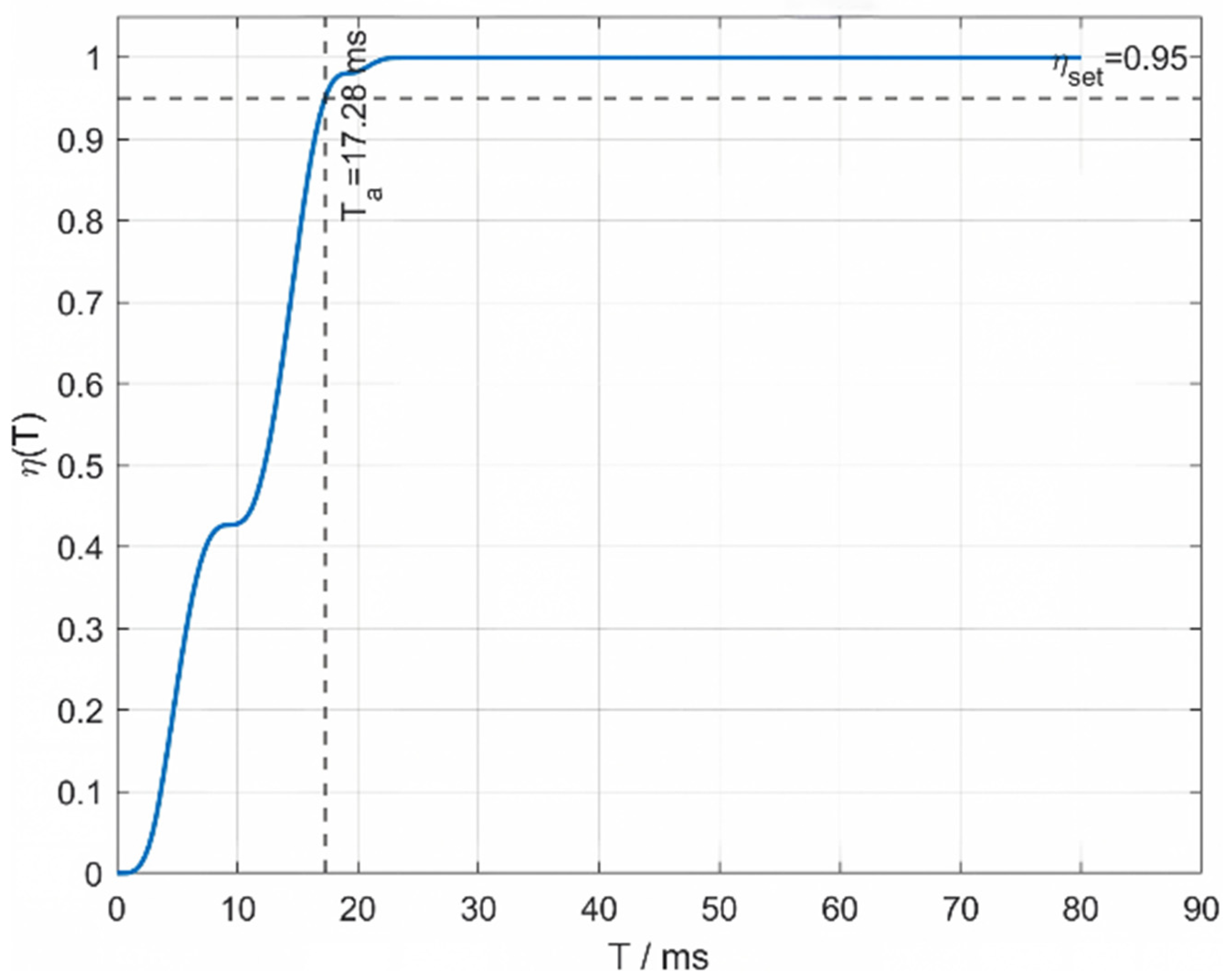
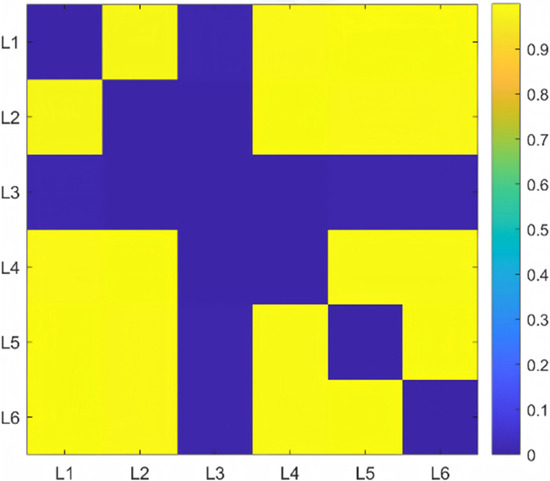
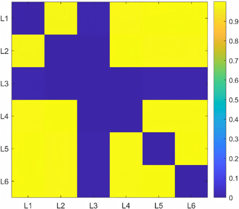
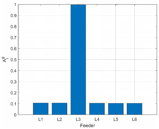
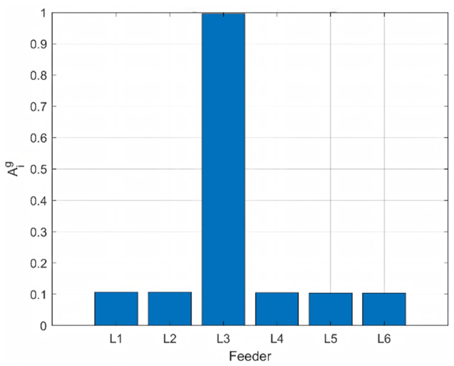
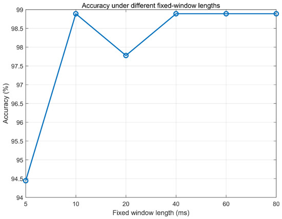
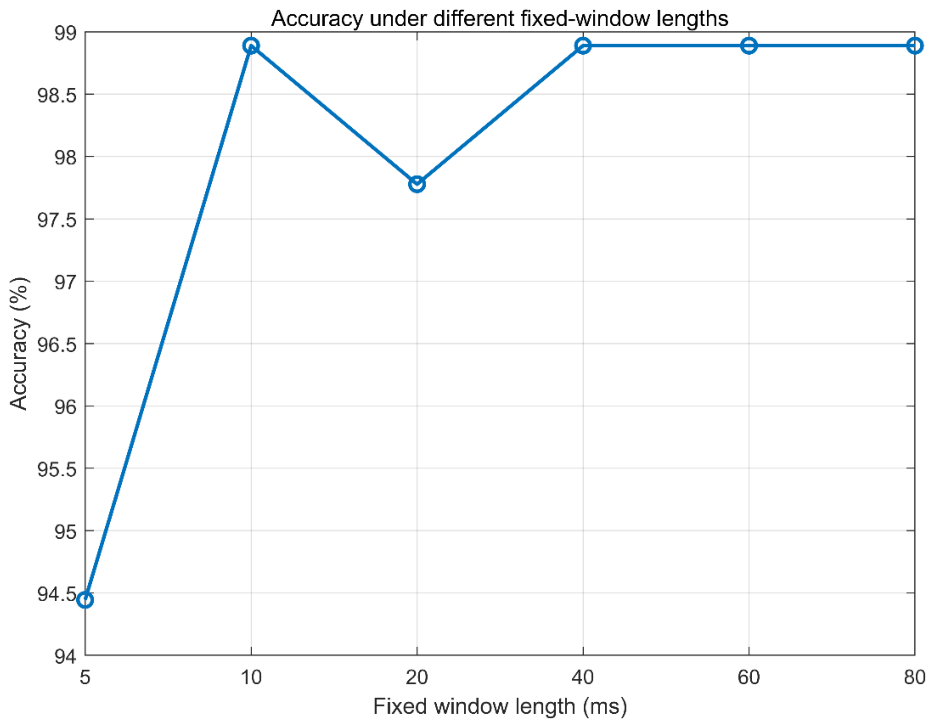
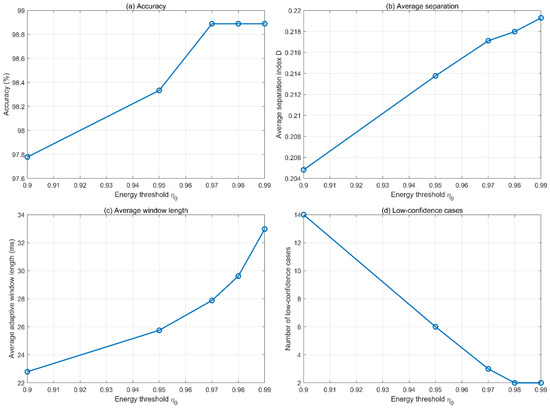
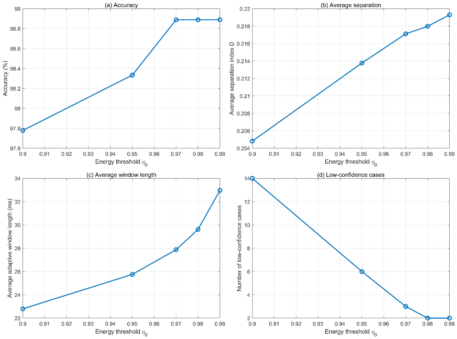
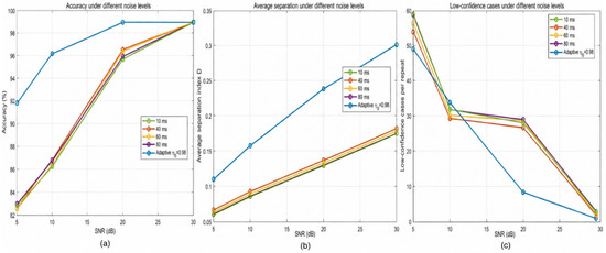
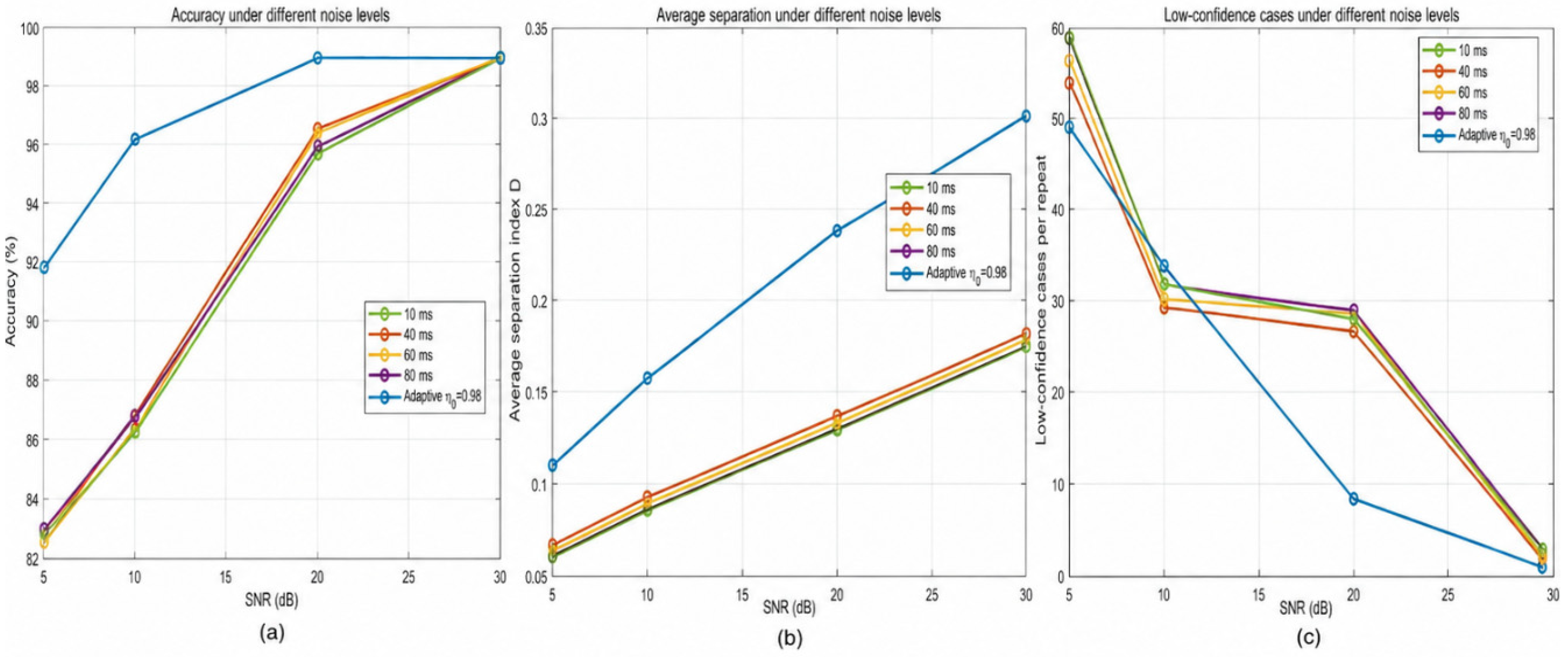
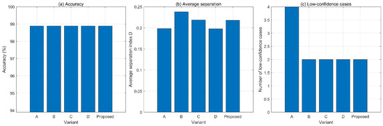
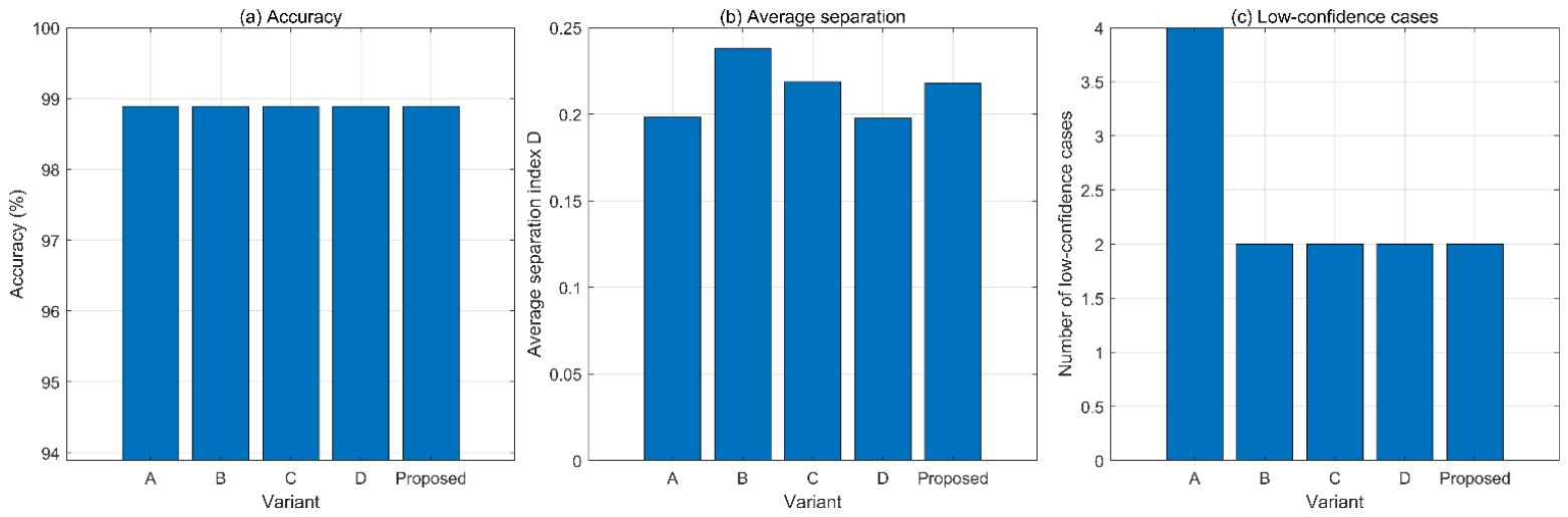

Disclaimer/Publisher’s Note: The statements, opinions and data contained in all publications are solely those of the individual author(s) and contributor(s) and not of MDPI and/or the editor(s). MDPI and/or the editor(s) disclaim responsibility for any injury to people or property resulting from any ideas, methods, instructions or products referred to in the content. |
© 2026 by the authors. Licensee MDPI, Basel, Switzerland. This article is an open access article distributed under the terms and conditions of the Creative Commons Attribution (CC BY) license.