Dynamic Leakage Characteristics and Emergency Shutdown Valve Optimization for Urban High-Pressure Gas Pipelines

Abstract

Addressing the lack of quantitative basis for dynamic response characterization and emergency shutdown decision-making in urban high-pressure gas pipeline leaks, this study takes a JS pipeline as the engineering case and establishes a dynamic simulation model based on OLGA incorporating leak and shutoff valve modules. The effects of aperture size, leak location, inlet flow rate, and valve operation on release intensity and economic losses are systematically analyzed. Results reveal that without intervention, leak-point pressure follows a four-stage evolution—steady operation, sharp drop, gradual decline to equilibrium, and post-plugging recovery—while leakage rate exhibits positively coupled synchronous behavior. Aperture size acts as an exponential-level hazard control factor; apertures ≥150 mm and rupture cases mandate immediate valve closure. Upstream leaks primarily threaten supply continuity, whereas downstream leaks exhibit sustained high-rate venting with greater release intensity, which may lead to more severe accident consequences depending on local atmospheric conditions and dispersion patterns. Inlet flow mainly modulates pressure equilibrium with limited influence on release rate. Emergency shutoff valves achieve loss reductions of 46.9–67.6% for apertures ≥150 mm, corresponding to savings of 0.47–3.48 million CNY within 4 h. These findings provide dynamic quantitative support for leak classification, coordinated valve control strategies, and emergency repair decision-making.

1. Introduction

Natural gas, as a clean and low-carbon fossil fuel, serves as the primary energy source for urban energy supply systems in China. Urban high-pressure gas pipelines are responsible for long-distance transmission from gate stations to city pressure-regulating stations, operating under high pressure and large flow rates. These pipelines traverse built-up areas with dense populations and complex structures, making any leakage prone to trigger major accidents such as fires, explosions, and toxic exposure, while also causing substantial venting losses and significant economic damage [1,2].

According to the European Gas Pipeline Incident Data Group (EGIG), global gas pipeline leakage incidents are classified into three categories: small holes, medium holes, and full ruptures, with orders-of-magnitude differences in release scale and hazard range across these categories [3]. In China, urban high-pressure pipelines are aging, and persistent threats from third-party damage, corrosion, welding defects, and geological subsidence have rendered leakage incidents increasingly frequent and complex [4]. Once a leak occurs, the in-pipe pressure and gas release rate evolve dynamically over time; upstream supply, shutoff valve actions, and repair operations further alter the leakage evolution pathway. Conventional steady-state formulas, which are valid only for static conditions, fail to capture the full time-varying leakage behavior and thus cannot support accurate risk assessment or emergency decision-making [5].

Quantitative estimation of leakage rate is a fundamental prerequisite for consequence modeling, risk classification, and emergency planning. Extensive studies have addressed gas pipeline leakage modeling and numerical simulation. Jo and Ahn [6] introduced a friction pressure loss correction factor to improve leakage calculations for high-pressure transmission pipelines. Montiel et al. [7] developed analytical formulas for full-scale leakage rates applicable to medium- and low-pressure pipelines. In China, Huo [8], Feng [9], and Wang [10] respectively compared the applicability of small- and large-hole models, derived simplified algorithms for mid-point leakage, and proposed subcritical/critical flow formulations, thus enriching the static leakage theory. Dong et al. [11] proposed a general CFD-based steady-state leakage model for long-distance pipelines covering a wide range of aperture sizes from pinholes to full-section fractures. In addition to leakage rate simulation, pipeline integrity management and repair safety research are also crucial for emergency leakage decision-making. In recent years, extensive research has been conducted on stress analysis of damaged pipelines: the study of stress distribution in pipelines repaired with composite coatings [12] revealed the mitigation mechanism of coating parameters on stress concentration in the damaged zone; the numerical model of the interaction between a mobile lift chain and a trunk pipeline during repair operations [13] provided a method for force analysis of pipelines during on-stream repair; the analytical model of the interaction between an oil pipeline and an overpass support in mountainous terrain [14] offered a theoretical tool for evaluating additional stresses on pipelines under complex terrain conditions. Furthermore, methods for girth weld defect assessment and repair decision-making [15] also provide important guidance for determining the feasibility of repairing defective pipelines. The above integrity studies indicate that emergency leakage decision-making is a multidisciplinary problem involving fluid mechanics, solid mechanics, and repair engineering. The dynamic leakage simulation in this study aims to provide accurate hydraulic boundary conditions and leakage source terms for this multidisciplinary decision-making framework.

Numerical simulation has become the mainstream approach for detailed leakage behavior analysis, with tools such as Fluent and OLGA commonly employed for single-scenario studies. Fu et al. [16] built an experimental platform to validate simulation accuracy for circular and rectangular orifices. Ebrahimi-Moghadam [17] used CFD to compare pressure field distributions for buried versus above-ground pipelines. Ji et al. [18] employed the VOF (Volume of Fluid) multiphase model to numerically simulate the diffusion process of porous leakage from underwater gas pipelines, and analyzed the effects of leakage velocity, aperture size, and water flow velocity on gas plume morphology, arrival time at the sea surface, and dispersion range. Jiang et al. [19] designed a full-scale experimental system to simulate small-hole leakage from high-pressure gas pipelines and observed methane dispersion in soil and atmosphere.

Despite these contributions, four major gaps remain: (i) most theoretical models are steady-state based and cannot describe the dynamic pressure-rate evolution under continuous urban supply; (ii) simulation scenarios are often isolated, lacking systematic multi-factor coupling of aperture, location, flow rate, and valve operation; (iii) quantitative economic loss evaluation under emergency control is absent; and (iv) the majority of studies focus on long-distance trunk lines, with little attention to urban high-pressure gas pipelines specifically.

To address these gaps, this paper presents the following innovations: a dynamic leakage simulation model is developed using OLGA, which reproduces the entire time-varying process from leakage initiation, steady venting, to plugging and recovery; multi-variable scenarios are designed to compare the effects of aperture, flow rate, leak location, and shutoff valve status, and to quantify the influence of each factor; market-based natural gas pricing is adopted to estimate economic losses under different scenarios, evaluate valve control effectiveness, and propose differentiated emergency strategies for small and large holes; and all parameters are derived from a real urban high-pressure pipeline, ensuring that the results are directly applicable to risk assessment and operational optimization.

2. Research Methodology

2.1. Mathematical Model for Steady-State Pipeline Leakage

2.1.1. Leakage Rate Calculation Model

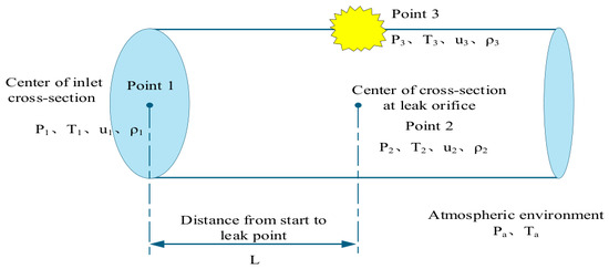
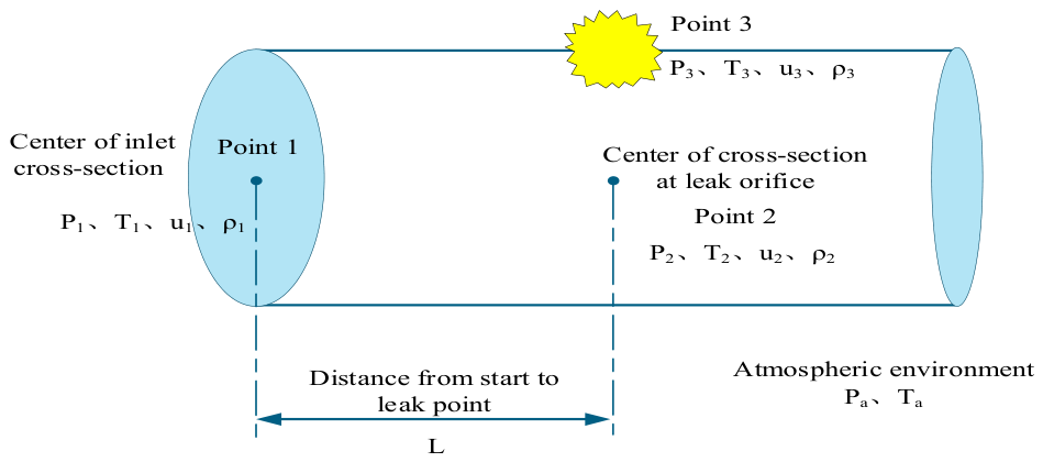
Currently, most commonly adopted leakage rate calculation methods are only applicable to steady-state continuous leakage scenarios or to the estimation of static oil/gas release rates after the simultaneous closure of emergency shutoff valves at both ends of the pipeline section [20]. In practice, the appropriate leak source model must be selected based on the aperture size of the gas pipeline leak. The internationally recognized typical models are generally classified into three categories: small-hole leakage, large-hole leakage, and pipeline rupture [21]. Figure 1 presents a simplified schematic of the gas pipeline leakage process, where points 1, 2, and 3 denote the center of the cross-section at the pipeline inlet, the center of the cross-section at the leak location, and the leak point, respectively; P, T, u, and ρ represent the pressure, temperature, gas velocity, and density at the corresponding positions, and L is the distance between the leak point and the pipeline inlet.

Figure 1. Simplified schematic of gas pipeline leakage.

(1) Small-hole leakage model

When the leak aperture is ≤20 mm, the small-hole leakage model can be used to calculate the gas release rate. This model determines the calculation method based on the gas flow regime, by comparing the critical pressure ratio (CPR) with the ratio of ambient pressure to the pressure at location 2 inside the pipe, thereby judging whether the flow is critical or subcritical. The critical pressure ratio (CPR) is given by Equation (1):

$$CPR={\displaystyle \frac{P_a}{P_2}}={\left({\displaystyle \frac{2}{k+1}}\right)}^{{\displaystyle \frac{k}{k+1}}}$$

(1)

where k is the adiabatic index, taken as 1.3 for natural gas; P₂ is the pressure at Point 2, and Pa is the ambient pressure, Pa.

When P_a/P₂ ≤ CPR, the gas flow at the leakage point is defined as critical flow, and the gas leakage rate is calculated by Equation (2):

$$Q_n=C_o{A}_n{P}_2\sqrt{{\displaystyle \frac{kM}{R{T}_{2}Z}}{({\displaystyle \frac{2}{k+1}})}^{{\displaystyle \frac{k+1}{k-1}}}}$$

(2)

When P_a/P₂ > CPR, the gas flow at the leakage point is defined as subcritical flow, and the gas leakage rate is calculated by Equation (3):

$$Q_m=C_o{A}_n{P}_2\sqrt{{\displaystyle \frac{2k}{k-1}}{\displaystyle \frac{M}{R{T}_{2}Z}}\left[{({\displaystyle \frac{P_a}{P_2}})}^{{\displaystyle \frac{2}{k}}}-{({\displaystyle \frac{P_a}{P_2}})}^{{\displaystyle \frac{k+1}{k}}}\right]}$$

(3)

where Q_m is the gas mass leakage rate, kg/s; C_o is the flow coefficient, ranging from 0.6 to 1.0; A_n is the leakage area, m; R is the universal gas constant, taken as 8.314 J/(mol·K) for natural gas; M is the molar mass of gas, kg/kmol; and Z is the gas compressibility factor, dimensionless.

(2) Large-Orifice Leakage Model

The large-orifice leakage model is adopted for calculation when the leakage aperture exceeds 20 mm and the pipeline remains unbroken. This model selects corresponding calculation formulas based on the flow state of gas inside the pipeline and at the leakage outlet, with the core procedure being the judgment of the critical flow state combination of the internal pipeline and the leakage outlet.

When the gas at internal pipeline Point 2 is in a subcritical flow state and the gas at leakage outlet Point 3 is in a critical flow state, the condition shown in Equation (4) is satisfied:

$$P_2\ge P_{1}M{a}_1\sqrt{{\displaystyle \frac{2+(k-1){{Ma}_1}^2}{k+1}}}$$

(4)

Under this condition, the gas leakage rate at the leakage outlet is calculated by Equation (5):

$$Q_m=C_o{A}_n{P}_2\sqrt{{\displaystyle \frac{kM}{R{T}_{2}Z}}{({\displaystyle \frac{2}{k+1}})}^{{\displaystyle \frac{k+1}{k-1}}}}$$

(5)

When the gas at both internal pipeline Point 2 and leakage outlet Point 3 is in a critical flow state, the condition shown in Equation (6) is satisfied:

$$P_2<P_{1}M{a}_1\sqrt{{\displaystyle \frac{2+(k-1){{Ma}_1}^2}{k+1}}}$$

(6)

Under this condition, the gas leakage rate at the leakage outlet is calculated by Equation (7):

$$Q_m=C_o{A}_n{P}_{1}M{a}_1\sqrt{{\displaystyle \frac{kM}{R{T}_{1}Z}}{({\displaystyle \frac{2}{k+1}})}^{{\displaystyle \frac{k+1}{k-1}}}}$$

(7)

where M_a is the Mach number, dimensionless.

(3) Pipeline Rupture Leakage Model

For the complete rupture condition of gas transmission pipelines, the flow state of the internal pipeline (Point 2) is consistent with that of the leakage point (Point 3). The mass flow rate at the leakage point is calculated by Equation (8):

$$Q_m=G{A}_n={\rho }_1{u}_1{A}_n={\rho }_2{u}_2{A}_n=C_o{A}_n\sqrt{{\displaystyle \frac{2M}{ZR}}{\displaystyle \frac{k}{k-1}}{\displaystyle \frac{T_2-T_1}{{\left(\frac{T_1}{P_1}\right)}^2-{\left(\frac{T_2}{P_2}\right)}^2}}}$$

(8)

2.1.2. Cumulative Leakage Mass Formula

For any leakage scenario, the leakage rate Q_m(t) is a time-dependent dynamic quantity. Over the time interval [t₁,t₂], the total mass of natural gas leaked into the environment, Mleak (in kg) can be obtained by integrating the leakage rate over time, as given in Equation (9):

$$M_{leak}={\displaystyle {\int }_{t_1}^{t_2}{Q}_m(t)dt}$$

(9)

In practical engineering calculations, when a discrete time step Δt is used, the cumulative leakage mass can be approximated by the summation in Equation (10):

$$M_{leak}\approx {\displaystyle \sum _{i=1}^n{Q}_{m,i}\cdot \Delta t_i}$$

(10)

where N is the total number of time steps; Q_m,i denotes the average leakage rate during the ith time step, and Δt is the constant duration of each step.

2.1.3. Conversion of Cumulative Mass to Standard Volume Equivalent

The leakage amount is typically expressed as the volume at standard conditions (101.325 kPa, 20 °C). Given the standard-condition density ρ_N of the leaked natural gas (in kg/Nm³), the standard volume corresponding to the cumulative mass is obtained by Equation (11).

The composition of the natural gas used in this study is shown in Table 1. The standard-condition density was calculated to be ρ_N = 0.717 kg/Nm³ (at 20 °C and 101.325 kPa). Therefore, all mass leakage quantities in this paper are converted to volume leakage quantities (in Nm³) using that density.

$$V_N={\displaystyle \frac{M_{leak}}{{\rho }_N}}$$

(11)

Table 1. Composition and volume fraction of the pipeline natural gas.

Gas Composition	C1	C2	C3	iC4	nC4	iC5	nC5	H2O	N2	CO2
Volume fraction (%)	94.18	3.56	1.12	0.28	0.32	0.01	0	0.01	0.42	0.10

2.2. OLGA Dynamic Leakage Simulation Modeling

2.2.1. Physical Model Setup

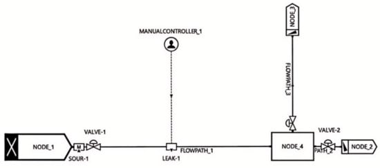
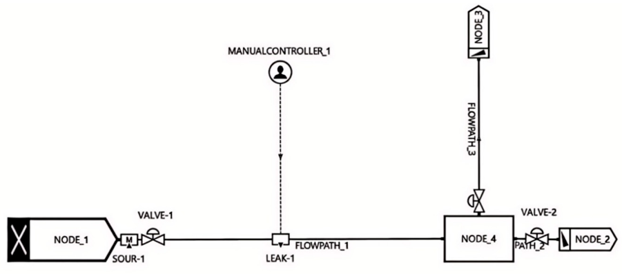
In this study, a dynamic leakage model for an urban high-pressure gas pipeline was developed using the OLGA software(Version 2023.4, Schlumberger, Stavanger, Norway). The model primarily consisted of six core components: an inlet flow node, the pipeline segment, emergency shut-off valves, a leak module, a pressure outlet, and a controller, as illustrated in Figure 2. In the model, the inlet flow node defined the flow rate and temperature conditions at the pipeline inlet, while the pressure outlet specified the pressure and temperature boundaries at the pipeline terminus. Key parameters such as pipeline routing mileage, internal wall roughness, and friction resistance coefficient were input into the pipeline module. The leak module was connected at the appropriate location along the pipeline to simulate leakage conditions. In OLGA, the leak orifice was implemented as a boundary outflow condition with a specified equivalent area and discharge coefficient, rather than as an additional pipe segment with an open end. The transient opening of the leak at t = 1 h was achieved through a controller-driven RAMP function that transitioned the leak area from zero to the target value over a 0.1 s interval; this smoothing strategy, combined with OLGA’s implicit time-integration scheme, effectively suppressed numerical oscillations while preserving the physical rapid depressurization characteristics. The controller was used to precisely control the opening/closing of the shut-off valves and the activation timing of the leak orifice, thereby enabling dynamic simulation of the leakage process and emergency response actions. The simulations were performed with a fixed time step of Δt = 0.01 s. A time-step independence study was conducted with five candidate time steps (0.1, 0.05, 0.02, 0.01, and 0.005 s); the results showed that for Δt ≤ 0.02 s, the relative deviations in peak leak pressure and steady-state leakage rate were below 1%, and the difference between Δt = 0.01 s and 0.005 s was less than 0.3%. Accordingly, Δt = 0.01 s was adopted as the optimal balance between accuracy and computational efficiency. The pipeline was discretized into approximately 210 segments with a spatial step of Δx ≈ 50 m, yielding a CFL number of approximately 0.084 (based on a sonic speed of ~420 m/s), which is well below the explicit stability limit and confirms that the transient pressure drop at leakage initiation is adequately resolved.

Figure 2. Dynamic leakage model of an urban high-pressure gas pipeline based on OLGA.

Since the study area was relatively flat and the pipeline burial depth remained approximately 1.5 m, the influence of actual terrain elevation changes was not considered in the model. It should be noted, however, that the JS pipeline is not perfectly flat; the actual elevation profile shows a maximum elevation difference of approximately 11 m (ranging from 474 m to 485 m) over the 10.5 km length. A comparative simulation incorporating the actual terrain profile was conducted for the 150 mm mid-point leak case. The results showed that including elevation changes led to deviations of less than 0.3% in steady-state pressure (1.731 MPa vs. 1.735 MPa) and leakage rate (28.135 kg/s vs. 28.190 kg/s) relative to the flat-terrain assumption. This negligible difference confirmed that the flat-terrain simplification was justified for this particular pipeline, as the 11 m elevation head was only ~0.5% of the 2.2 MPa operating pressure.

It should be noted that reverse flow was explicitly permitted at the downstream pressure-outlet boundary. In the early stage of leakage (approximately the first 30 s), a localized low-pressure zone forms around the leak point, which may induce a small amount of reverse flow at the downstream boundary. However, this reverse flow has a negligible effect on the overall mass balance. Furthermore, the “dynamic equilibrium” defined in this paper refers to a flux-balance state in which, under continuous upstream gas supply, the net difference between the leakage rate and the upstream replenishment becomes constant, thereby maintaining a stable leak-point pressure. This is fundamentally different from a static equilibrium in the traditional sense.

2.2.2. Study Object and Process Parameters

The subject of this study was the JS high-pressure gas pipeline, which has a total length of approximately 10.5 km, extending from the gate station to the urban pressure-regulating station. The surrounding soil is predominantly silty clay, with the following thermal properties used in the OLGA model: thermal conductivity λ_soil = 1.5 W/(m·K), specific heat capacity c_p,soil = 1200 J/(kg·K), and density ρ_soil = 1800 kg/m³. The pipeline has an outer diameter of 406.4 mm and a wall thickness of 9.5 mm. The design pressure is 3.0 MPa, and the current operating pressure is 2.2 MPa. The pipeline was manufactured from L360M (PSL2 grade) line pipe steel, Inner Mongolia Baotou Steel Union Co., Ltd., Baotou, Inner Mongolia Autonomous Region, China. The composition (volume fractions) of the transported natural gas is given in Table 1, and the main operating parameters of the pipeline are listed in Table 2.

Table 2. Main operating parameters of the urban high-pressure gas pipeline.

Parameter	Value	Parameter	Value
Pipe diameter	D406.4 × 9.5 mm	Outlet temperature	20 °C
Total pipeline length	10.5 km	Heat transfer coefficient	2.8 W/m2·K
Design pressure	3.0 MPa	Pipe internal wall roughness	0.00012 m
Operating pressure	2.2 MPa	Inlet flow rate (baseline)	15,000 Nm3/h
Inlet temperature	24 °C

2.2.3. Design of Dynamic Leakage Simulation Scenarios

Based on the leak orifice classification criteria specified in API 581-2020 Risk-Based Inspection Methodology [22] and GB/T 34346-2017 Guidelines for Risk-Based Hazard Classification of Oil and Gas Pipelines [23], and in consideration of the actual leakage types encountered in urban high-pressure gas pipelines, leak orifice sizes are classified into four levels: pinhole leak, medium-hole leak, large-hole leak, and pipeline rupture. Correspondingly, five specific leak dimensions were considered: 8 mm, 20 mm, 50 mm, 150 mm, and 387.4 mm (the internal diameter of the pipeline).

Urban gas flow rates exhibit significant temporal non-uniformity, with flow rates varying dynamically over time and being strongly influenced by end-user consumption patterns. This study therefore incorporated the effects of different inlet flow rate conditions on leakage dynamics.

For pinhole-leak scenarios, hot-tapping or on-stream sealing repair can be performed without interrupting normal pipeline transmission. When the in-pipe pressure drop rate exceeds the preset threshold of the mainline emergency shut-off valves, the valves at both the upstream and downstream ends of the pipeline will automatically interlock and close. On-site operators are required to promptly initiate the emergency response plan and implement corresponding emergency measures. This study also analyzed the impact of shut-off valve closure on the leakage consequences. The detailed leakage scenarios are summarized in Table 3. In the OLGA model, the parameters for emergency-shutdown valve closure are shown in Table 4.

Table 3. Design of dynamic leakage scenarios.

Scenario Feature	Dynamic Scenario Description	Scenario Feature	Dynamic Scenario Description
Different leak orifice diameters (mm)	Pinhole leak (8, 20) Medium-hole leak (50) Large-hole leak (150) Pipeline rupture (387.4)	Different inlet flow rates (m3/h)	6000
			10,500
			15,000
			21,000
			28,000
Different leak locations (km)	Upstream (1.5, 3.0) Midstream (5.25) Downstream (7.5, 9.0)	Effect of emergency shut-off valves	Closure of emergency shut-off valves upstream and downstream of the leak section

Table 4. Parameters of emergency-shutdown valve closure in the OLGA model.

Parameter	Value	Description
Triggering threshold	Pressure drop rate ≥ 0.1 MPa/s	Based on SCADA field data
Detection delay	3 s	Includes signal acquisition, transmission, and confirmation
Closure mode	Linear (RAMP)	Avoids water hammer
Closure duration	10 s	Linear transition from fully open to fully closed
Closure initiation	1.5 h after leakage	Accounts for operational confirmation time
Valve stroking law	θ(t) = θ0·(1 − t/Tc), 0 ≤ t ≤ Tc	Linear closure; θ0 = 1 (fully open), Tc = 10 s
Water hammer assessment	ΔPmax ≈ 0.3–0.5 MPa	Below design pressure (3.0 MPa); safe

It should be noted that controlled-leakage experiments cannot be performed on in-service high-pressure pipelines, so direct comparative validation against field-measured leakage data was not carried out in this study. Nevertheless, OLGA is a widely used industry-standard transient multiphase flow simulator, and its leakage-simulation capability has been validated in multiple independent studies. Ma et al. [24] established a calculation model consistent with experimental conditions using OLGA based on industrial-scale supercritical CO₂ pipeline leakage tests. The results showed that the average calculation errors of OLGA for pressure were 15.3% and 14.7%, while the simulation errors for temperature were 21.2% and 24.5%. Such error ranges satisfy the requirements of engineering practice. Furthermore, the reliability of the present model was guaranteed from three aspects: (1) the model was built on the actual operating parameters of the JS pipeline (Table 1) and natural-gas composition (Table 2) to ensure realistic boundary conditions; (2) independence verification was performed for time-step sizes (0.1, 0.05, 0.02, 0.01, 0.005 s) and spatial meshes (100–500 segments), ensuring negligible numerical discretization errors; (3) mass-balance accounting verified the physical consistency of the model during the steady-state leakage phase. Considering parameter-value errors (±5–10%), uncertainty in the orifice discharge coefficient (C₀ = 0.6–1.0), and simplifications introduced by the one-dimensional model, the overall uncertainty of the proposed model for steady-state leakage-rate prediction was estimated to be ±15–20%, which falls within the acceptable range for engineering decision-making.

3. Results and Discussion

3.1. Four-Stage Evolution Pattern of the Full Leakage Process Under Baseline Conditions

To investigate the fundamental evolution of leak-point pressure and leakage rate in an urban high-pressure gas pipeline, a baseline simulation case was defined as follows: the leak point was located at the midpoint of the total pipeline length, 5.25 km from the upstream end, with a leak orifice diameter of 150 mm and an inlet flow rate of 15,000 Nm³/h. It was assumed that no process control measures were implemented after leakage initiation, and the pipeline remained under pressurized operating conditions. The total simulation duration was 4 h, with leakage starting at the first hour and being successfully sealed off by maintenance personnel at the third hour.

3.1.1. Temporal Response of Leak-Point Pressure

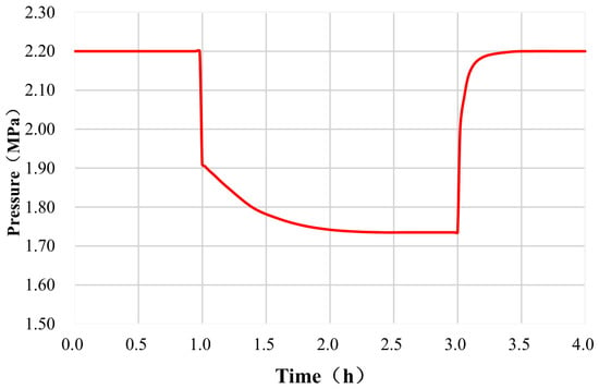
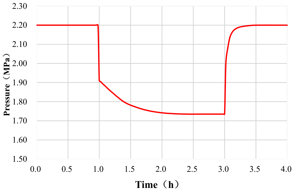
The leak-point pressure in an urban high-pressure gas pipeline evolves through four distinct stages. The pressure data for each stage are summarized in Table 5, and Figure 3 presents the dynamic evolution of leak-point pressure over time.

Table 5. Four-stage pressure evolution parameters at leakage point under base-case conditions (150 mm hole, midpoint leakage, 15,000 Nm³/h, valve open).

Stage	Time Interval	Pressure Range	Characteristics
Steady-state operation	0~1.0 h	2.200 MPa (constant)	Supply-demand balance maintained; pipeline network in steady-state transmission
Abrupt sharp drop	1.0 h (instantaneous)	2.200 → 1.910 MPa	Instantaneous pressure drop of 0.290 MPa (13.18%)
Gradual decline to steady state	1.0~3.0 h	1.910 → 1.735 MPa	Decline rate gradually slows; final stabilization at 1.735 MPa
Rapid recovery after plugging	3.0~4.0 h	1.735 → 2.200 MPa	Pressure progressively returns to the initial value

Figure 3. Pressure evolution at leakage point under base case condition (150 mm hole, midpoint leakage, 15,000 Nm³/h, valve open).

(1) Steady-state operation stage (0–1 h): No leakage path exists. The gas supply and demand are balanced along the pipeline. The leak-point pressure remains stable at 2.100 MPa (the actual operating pressure at this location after accounting for the frictional pressure drop along the pipeline), and the pipeline network is in a steady-state transmission condition.

(2) Abrupt sharp-drop stage (instantaneous at 1 h when leakage occurs): At the moment the leak channel opens (over a 0.1 s RAMP transition period), the high-pressure gas inside the pipeline rapidly escapes to the atmosphere. The leak-point pressure experiences a rapid, near-instantaneous (on the engineering time scale) cliff-like drop, falling from 2.200 MPa to 1.910 MPa within approximately 0.1 s, corresponding to an instantaneous pressure decrease of 0.290 MPa (13.18%). With a time step of Δt = 0.01 s and an output sampling interval of 0.1 s, the transient is resolved within 10 computational steps; the corresponding pressure-wave transit time from the mid-point leak to the pipe end is approximately 12.5 s (based on a sonic speed of 420 m/s), which is resolved within over 1200 time steps, ensuring that the dynamic response is accurately captured.

(3) Gradual slow-decline stage (1 h to 3 h): The rate of pressure decline continuously decreases and eventually stabilizes at a dynamic equilibrium value of 1.735 MPa. The gas flow rate supplied from the upstream source balances the venting leakage flow rate, establishing a new pressure equilibrium in the pipeline network. No further continuous pressure decay is observed.

(4) Rapid recovery stage after plugging (after completion of sealing at 3 h): The leakage path is blocked, and no gas is vented. The pressure recovers rapidly, with the recovery rate gradually slowing down as the pressure approaches its initial value. The pressure fully returns to the initial operating pressure of 2.200 MPa within the time interval from 3 h to 4 h.

The core logic of the pressure evolution can be summarized as follows: the instantaneous pressure differential at the onset of leakage drives gas release; upstream supply replenishment offsets a portion of the pressure loss, leading to a new steady state; upon sealing, the venting path is cut off and the pipeline pressure reverts to its original steady-state condition.

3.1.2. Coupled Evolution Characteristics of Leakage Rate

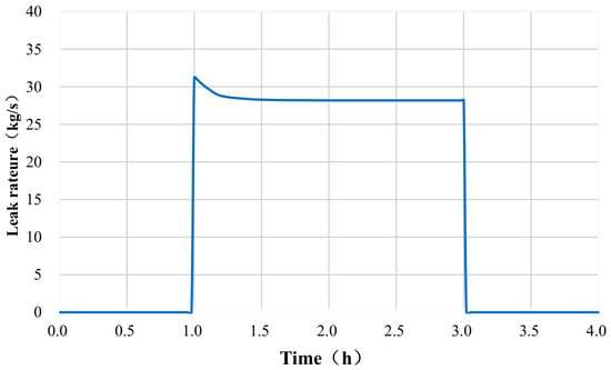
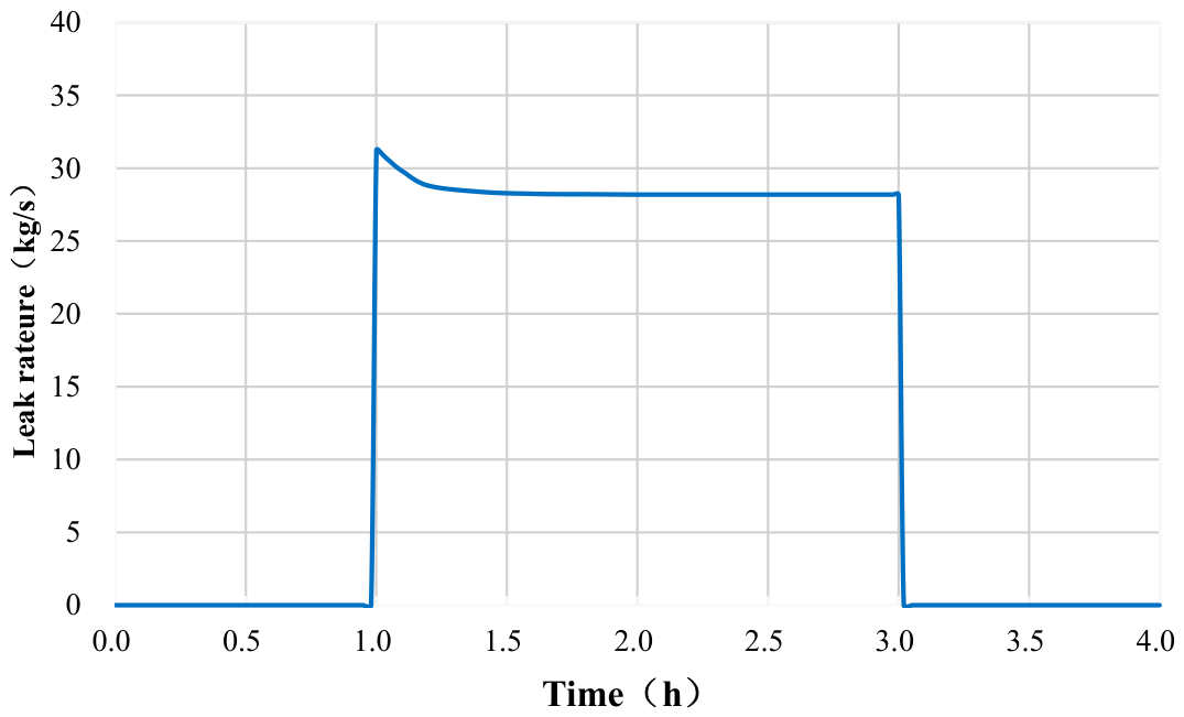
The temporal variation of the leakage rate is fully synchronized with the pressure evolution and also exhibits four corresponding stages. The four-stage parameters of the leakage rate under the baseline condition are summarized in Table 6, and Figure 4 presents the general temporal pattern of the leakage rate at the leak point.

Table 6. Four-stage leakage rate evolution parameters under base case condition (150 mm hole, midpoint leakage, 15,000 Nm³/h, valve open).

Stage	Time Interval	Leakage Rate Range	Characteristics
Zero leakage	0–1.0 h	0 kg/s	No leakage path
Instantaneous peak surge	1.0 h (instantaneous)	0 → 31.247 kg/s	Driven by pressure differential; instantaneous surge to peak
Exponential decay to steady state	1.0–3.0 h	31.247 → 28.190 kg/s	Gradual decay as pressure declines
Return to zero after plugging	3.0 h (instantaneous)	28.190 → 0 kg/s	Leakage path sealed; instantaneous termination

Note: A transient intermediate value of 17.998 kg/s was observed at approximately 0.5 s after leakage initiation (non-steady-state value); the steady-state value of 28.190 kg/s was established approximately 3–5 s after leakage onset.

Figure 4. Leakage rate evolution under base-case conditions (150 mm hole, midpoint leakage, 15,000 Nm³/h, valve open).

(1) Zero-leakage stable stage (0–1 h): With no leak orifice present, the leakage rate remains constant at zero.

(2) Abrupt peak-rise stage (instantaneous at leakage initiation): The large pressure differential between the inside and outside of the pipeline provides an extremely strong driving force, causing the leakage rate to surge instantaneously to a peak value of 31.247 kg/s.

(3) Exponential decay to steady-state stage (1–3 h): As the leak-point pressure continues to decrease slightly, the driving force for leakage weakens, and the leakage rate gradually declines until it finally stabilizes at a constant value of 28.190 kg/s approximately 5 s after leakage initiation (it should be noted that a transient intermediate value of 17.998 kg/s exists at approximately 0.5 s after leakage onset; this value is not the steady-state value). The pressure and leakage rate exhibit a positive coupling relationship.

(4) Termination and return-to-zero stage (after plugging at 3 h): The leakage path is completely sealed, and the leakage rate drops instantaneously to zero, marking the complete termination of the venting process.

The pressure and leakage rate exhibit a positive coupling relationship: a higher in-pipe pressure corresponds to a stronger leakage driving force and thus a higher steady-state leakage rate; a dynamic pressure equilibrium corresponds to a constant venting leakage rate.

3.1.3. Transient Mass-Balance Verification for the Baseline Case

To further validate the physical consistency of the four-stage evolution model described above, a mass-balance analysis was performed for the steady leakage stage (1–3 h) of the baseline case (150 mm orifice, midpoint leakage, 15,000 Nm³/h, valves open). As shown in Table 7, after the dynamic equilibrium was established, the upstream boundary inflow was 3.857 × 10⁵ kg; of this, 2.918 × 10⁵ kg (75.7%) was lost through the leak orifice, and 9.39 × 10⁴ kg (24.3%) exited through the downstream pressure outlet. The change in pipeline linepack approached zero under steady-state conditions. These results are in strict agreement with the continuity equation, confirming the accuracy of the OLGA dynamic model in capturing the coupled relationship among upstream replenishment, leakage loss, and downstream outflow. It is worth noting that during the initial transient phase (approximately the first 30 s), a small amount of reverse flow (peak value ~0.5 kg/s) was observed at the downstream boundary, caused by the localized low-pressure zone around the leak point before the upstream pressure wave fully compensated for it; however, this reverse flow accounted for less than 0.05% of the total leakage volume and did not affect the macroscopic mass-balance conclusions.

Table 7. Mass balance accounting for the baseline case (steady leakage stage, 1–3 h).

Mass Balance Item	Mass (kg)	Percentage
Upstream boundary inflow	3.857 × 105	100%
Leakage loss	2.918 × 105	75.7%
Downstream outlet outflow	9.39 × 104	24.3%
Change in pipeline linepack	≈0 (steady state)	—

3.2. Effect of Leak Orifice Diameter on Time-Varying Leakage Characteristics

Under the conditions of an inlet flow rate of 15,000 Nm³/h, leakage at the pipeline midpoint, and without closure of the emergency shut-off valves, five orifice sizes (8 mm, 20 mm, 50 mm, 150 mm, and 387.4 mm) were set to investigate the influence of leak orifice diameter on the time-varying leakage behavior.

3.2.1. Effect of Leak Orifice Diameter on Leak-Point Pressure

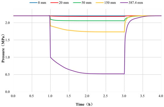
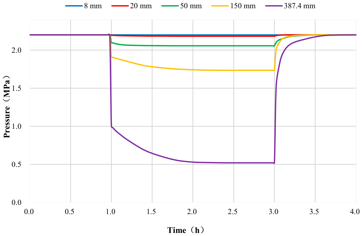
Figure 5 presents the pressure time-history curves for different leak orifice diameters, and Table 8 summarizes the corresponding pressure variation parameters.

Figure 5. Pressure evolution at leakage point for different hole diameters (midpoint leakage, 15,000 Nm³/h, valve open).

Table 8. Pressure variation parameters for different hole diameters (midpoint leakage, 15,000 Nm³/h, valve open).

Leak Orifice Diameter (mm)	Minimum Steady-State Pressure (MPa)	Absolute Pressure Drop (MPa)	Relative Pressure Drop (%)	Pressure Disturbance Characteristics
8	2.199	0.0012	0.055	Pipeline pressure virtually unchanged; on-stream repair feasible
20	2.183	0.0168	0.76	Slight pressure drop; mainline transmission unaffected
50	2.057	0.1435	6.52	Moderate pressure decay; downstream gas supply requires attention
150	1.735	0.4650	21.14	Significant pressure drop; severe shortage of downstream gas supply
387.4	0.521	1.6790	76.32	Pipeline network nearly depressurized; gas supply completely interrupted

As can be seen from Figure 5 and Table 8, the leak orifice diameter is the decisive factor determining the degree of pressure disturbance in the pipeline network. The orifice diameter exhibits an exponential positive correlation with the pressure drop magnitude. For an 8 mm pinhole leak, the minimum steady-state pressure is 2.199 MPa, with a relative pressure drop of only 0.055%, indicating virtually no disturbance to the pipeline pressure. For the 20 mm orifice, the relative pressure drop is 0.76%, resulting in a slight pressure decline that does not affect the mainline transmission. For the 50 mm medium-sized leak, the relative pressure drop reaches 6.52%, showing a moderate pressure reduction that requires close attention to downstream gas supply. For the 150 mm large-hole leak, the steady-state pressure drops to 1.735 MPa, with a relative pressure drop of 21.14%, causing a substantial drop in the operating pressure and resulting in a severe shortage of downstream supply. In the case of a complete pipeline rupture (387.4 mm), the minimum steady-state pressure is only 0.521 MPa, corresponding to a relative pressure drop as high as 76.32%, indicating that the pipeline network nearly loses its pressure and gas supply is completely interrupted.

During the recovery stage after plugging (3–4 h), the pressure for all orifice sizes returns to the initial value of 2.200 MPa. Although larger orifices exhibit a steeper recovery gradient at the initial stage, the overall recovery time remains essentially the same across all cases. The above observations indicate that for small-hole leaks (≤20 mm), normal pipeline transmission can be maintained, and on-stream (hot-tap) repairs can be performed. For large-hole leaks (≥150 mm) and rupture scenarios, emergency shutdown must be initiated immediately.

It should be emphasized that the above judgment regarding the “feasibility of on-stream repair” is limited to the hydraulic acceptability level, i.e., for leakage orifice diameters ≤20 mm, the pipeline can still maintain normal transmission pressure and the leakage rate is controllable. However, the mechanical safety of on-stream repair involves multiple factors, including defect type and geometry, remaining wall thickness, local stress state, girth weld defect assessment, and the applicability of specific repair techniques (such as clamp sealing, composite repair, and in-service welding). Actual engineering decisions must be made based on hydraulic analysis combined with comprehensive assessments using pipeline integrity evaluation and repair technology codes (e.g., SY/T 6649, API RP 2201). The hydraulic analysis results of this study provide boundary conditions (pressure, temperature, flow rate) for subsequent mechanical safety evaluations but should not be misinterpreted as a complete conclusion on the safety of on-stream repair.

3.2.2. Effect of Leak Orifice Diameter on Leakage Rate and Total Release Volume

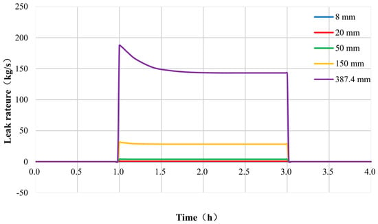
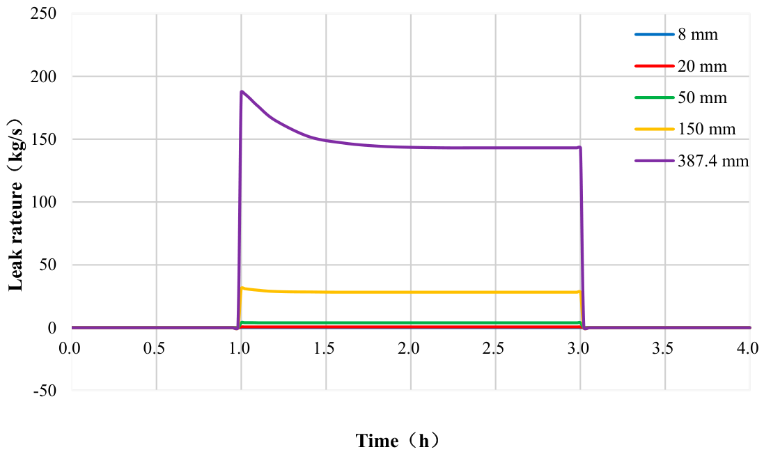
Figure 6 presents the time-history curves of leakage rate for different orifice diameters, and Table 9 summarizes the corresponding leakage rate and total release volume parameters. Analysis of Figure 6 and Table 9 reveals that the leakage rate is approximately proportional to the flow area of the leak orifice; however, owing to the dynamic pressure decay in the pipeline network, the actual increase in leakage rate for large-diameter orifices is lower than the theoretical value based on area ratio. For the 20 mm orifice, the area is 6.25 times that of the 8 mm orifice, and the steady-state leakage rate ratio is 6.26, indicating good agreement. For the 150 mm orifice, the area is nine times that of the 50 mm orifice, but the steady-state leakage rate ratio is only 7.23, significantly lower. This is attributed to the 21.14% pressure drop caused by the 150 mm leak, which substantially weakens the driving pressure differential. For the 387.4 mm rupture case, the area is 6.67 times that of the 150 mm orifice, yet the leakage rate ratio is only 5.08; under rupture conditions, the pipeline network is nearly depressurized (pressure drop of 76.32%), and the mass flux per unit area decreases significantly. These proportional relationships indicate that for large-diameter leaks, the sharp drop in in-pipe pressure induces a “pressure-drop self-feedback” effect that weakens the leakage driving force and curbs the rate of increase in leakage rate. Notably, this feedback effect exhibits a threshold behavior: when the pressure drop is below approximately 5% (as in the 20 mm vs. 8 mm case, where the pressure drop is only 0.76%), the reduction in driving pressure is negligible, and the leakage rate remains essentially proportional to the orifice area (6.25 vs. 6.26). However, when the pressure drop exceeds 5% (as in the 150 mm vs. 50 mm case, where the pressure drops are 21.14% and 6.52%, respectively), the feedback effect becomes significant, causing the leakage rate ratio (7.23) to fall substantially below the area ratio (9.0). This threshold behavior has practical engineering implications: for small-hole leaks with pressure drops below 5%, simplified linear area-ratio estimation is acceptable; for large-hole leaks exceeding this threshold, nonlinear pressure-feedback models must be employed.

Figure 6. Leakage rate evolution for different hole diameters (midpoint leakage, 15,000 Nm³/h, valve open).

Table 9. Leakage rate and total release volume for different hole diameters (midpoint leakage, 15,000 Nm³/h, valve open).

Leak Orifice Diameter (mm)	Peak Rate (kg/s)	Steady-State Average Rate (kg/s)	Total Release Volume (1–3 h) (kg)	Equivalent Release Volume (Nm3)	Characteristics of Rate Variation
8	0.103	0.102	734	1024	Extremely low throughout; negligible venting
20	0.647	0.639	4600	6417	Low steady-state venting; limited short-term loss
50	4.038	3.900	28,080	39,172	Moderate venting; emergency response required
150	31.247	28.190	202,968	283,140	Significant peak; sustained large-volume release
387.4	187.536	143.082	1,030,190	1,437,115	Instantaneous peak near 190 kg/s; maximum total release

From an engineering risk perspective, for small-hole leaks of 8 mm and 20 mm, the leakage rate is extremely low (peak ≤ 0.647 kg/s), and the cumulative leakage over 1–3 h is less than 4600 kg, corresponding to an economic loss that is manageable (≤23,000 RMB), thus providing a sufficient time window for on-stream sealing operations. For large-hole leaks (≥150 mm) and rupture scenarios, the peak leakage rate ranges from 31.247 to 187.536 kg/s, and the release volume over 1–3 h reaches 2.831 × 10⁵ to 1.437 × 10⁶ Nm³. Given the extremely high instantaneous release intensity, a level-1 emergency response must be activated immediately, and interlocking closure of the emergency shut-off valves must be implemented.

It should be clarified that the 387.4 mm (pipeline internal diameter) opening in this study simulates a circular opening with an area equivalent to the internal cross-section of the pipe, representing an extreme leakage event with complete loss of the pipe cross-section. In an actual full-bore rupture, two open ends are formed at the fracture, resulting in bidirectional leakage and complex transient wave interactions. Due to the one-dimensional nature of OLGA, the 387.4 mm single-orifice simulation was adopted as a conservative engineering approximation. The rationale for this simplification is threefold: (1) for emergency valve control strategy optimization, the total release volume and pressure decay trend are the decisive factors, and the difference between bidirectional and unidirectional leakage is acceptable within a conservative estimation framework; (2) although OLGA’s one-dimensional framework cannot precisely resolve the complex three-dimensional flow field at the fracture ends, its order-of-magnitude prediction capability is sufficient for engineering decision-making; and (3) the “rupture scenario” in this study is intended to provide an upper-bound estimate of leakage consequences for emergency response under the most adverse conditions. For accurate analysis of the near-field flow field and wave dynamics at the fracture, complementary three-dimensional CFD simulations would be required.

3.3. Differential Effects of Leakage Location on Time-Varying Leakage Characteristics

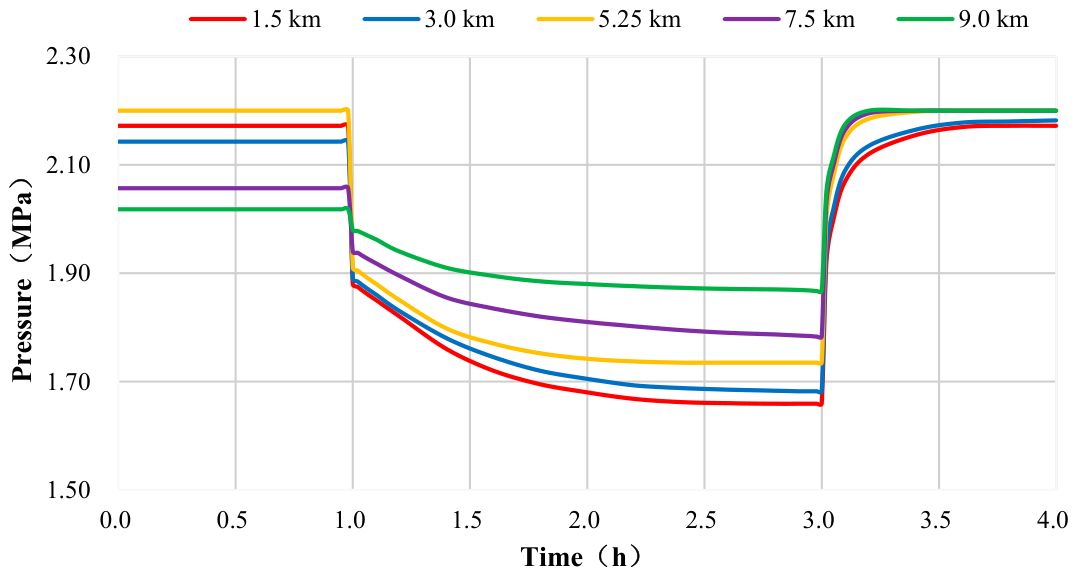
With a fixed orifice diameter of 150 mm, an inlet flow rate of 15,000 Nm³/h, and without closure of the emergency shut-off valves, five locations along the pipeline (1.5 km, 3.0 km, 5.25 km, 7.5 km, and 9.0 km from the upstream end) were selected to investigate the effect of leakage position. Owing to the natural pressure gradient caused by frictional resistance along the pipeline, the initial pressure at the leak point varies with location, which in turn leads to distinctly different evolution patterns throughout the entire leakage process.

3.3.1. Effect of Leakage Location on Pipeline Network Pressure Attenuation

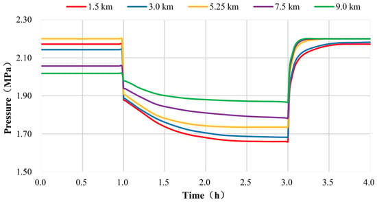
Figure 7 presents the pressure time-history curves for different leakage locations, and Table 10 summarizes the corresponding quantitative parameters. Figure 7 and Table 10 reveal the differential effects of leakage location on pressure disturbance in the pipeline network. The initial operating pressures at the five leakage locations are 2.172 MPa at 1.5 km, 2.143 MPa at 3.0 km, 2.100 MPa at 5.25 km, 2.057 MPa at 7.5 km, and 2.018 MPa at 9.0 km from the upstream end. All values were obtained from steady-state hydraulic calculations that fully accounted for the frictional pressure drop along the pipeline, rather than simply adopting a uniform design pressure value.

Figure 7. Pressure evolution at leakage point for different leakage locations (150 mm hole, 15,000 Nm³/h, valve open).

Table 10. Pressure variation parameters for different leakage locations (150 mm hole, 15,000 Nm³/h, valve open).

Leakage Location (km)	Initial Operating Pressure (MPa)	Minimum Steady-State Pressure (MPa)	Absolute Pressure Drop (MPa)	Relative Pressure Drop (%)	Pressure Disturbance Characteristics
1.5 (upstream)	2.172	1.659	0.513	23.62	Leakage in upstream high-pressure zone; largest pressure drop
3.0	2.143	1.682	0.461	21.51	Upper-middle section; moderately large pressure drop
5.25 (midpoint)	2.100	1.735	0.365	17.38	Midpoint of pipeline; moderate pressure drop
7.5	2.057	1.871	0.186	9.04	Downstream section; significantly reduced pressure drop
9.0 (downstream)	2.018	1.984	0.034	1.68	Near the pipeline terminus; pressure virtually unchanged

Following leakage initiation, the upstream location at 1.5 km exhibits the largest pressure drop (0.513 MPa, corresponding to a relative drop of 23.62%). This is because an upstream leak is close to the gas source and the pipe segment has a relatively small gas storage capacity; once the leakage venting occurs, the incoming flow from the upstream source cannot replenish the lost gas in a timely manner, causing the pressure to drop rapidly. This pressure reduction propagates downstream via pressure waves, affecting the entire pipeline. In contrast, at the downstream location of 9.0 km, the pressure drop is only 0.034 MPa (relative drop of 1.68%). The leak point is located immediately upstream of the pressure-regulating station, where a strong back-pressure support exists. Moreover, the long upstream pipe section provides a large buffer capacity, and the overall pipeline pressure remains virtually undisturbed.

Engineering risk implications: Leakage in the upstream pipe section (0–3 km) poses the most severe hazard, as a large-hole leak in this region can lead to gas supply instability across the entire mainline. Consequently, third-party construction protection and corrosion inspection should be particularly reinforced in this zone. Although leakage in the downstream section (7–10 km) has a minor effect on pipeline pressure, the venting duration is longer; therefore, emphasis should be placed on rapid leak detection and the response speed of shut-off valves.

3.3.2. Effect of Leakage Location on Leakage Venting Rate

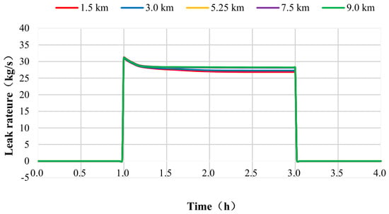
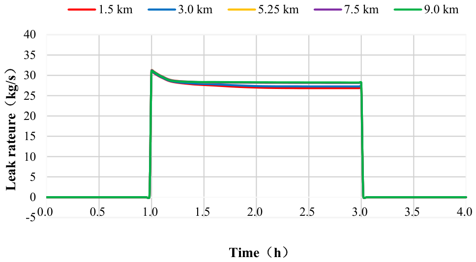
Figure 8 presents the leakage-rate time-history curves for different leakage locations, and Table 11 summarizes the quantitative parameters. Figure 8 and Table 11 demonstrate that the closer the leak point is to the downstream end, the higher the steady-state leakage rate and the smaller the rate attenuation.

Figure 8. Leakage rate evolution for different leakage locations (150 mm hole, 15,000 Nm³/h, valve open).

Table 11. Leakage rate parameters for different leakage locations (150 mm hole, 15,000 Nm³/h, valve open).

Leakage Location (km)	Peak Leakage Rate (kg/s)	Steady-State Leakage Rate (kg/s)	Rate Reduction (%)	Characteristics of Rate Evolution
1.5 (upstream)	30.873	26.847	13.04	Significant rate decay after leakage; lowest steady-state rate
3.0	30.965	27.329	11.74	Relatively large attenuation
5.25 (midpoint)	31.247	28.190	9.78	Baseline case
7.5	31.198	29.442	5.63	Weak attenuation
9.0 (downstream)	31.054	30.578	1.53	Rate nearly constant; maximum steady-state venting

At the upstream location of 1.5 km, the steady-state leakage rate is 26.847 kg/s (rate reduction of 13.04%), whereas at the downstream location of 9.0 km, it is 30.578 kg/s (rate reduction of only 1.53%), representing a difference of 3.731 kg/s (approximately 13.9%). The underlying reason for this pattern is as follows: Upstream leakage causes a substantial drop in the overall pipeline pressure (0.513 MPa pressure drop), leading to a sharp decrease in the pressure differential at the leak point and consequently a severely weakened leakage driving force. Conversely, downstream leakage induces only a negligible pressure disturbance (0.034 MPa drop), and the pressure at the leak point remains relatively high (between 2.018 and 1.984 MPa), maintaining a stable pressure differential and thus sustaining a high venting rate.

In terms of rate curve morphology, the upstream location exhibits a “steep-decline” pattern, where the peak rate of 30.873 kg/s rapidly decreases to a steady-state value of 26.847 kg/s. In contrast, the downstream location shows a “flat” pattern, with the peak rate of 31.054 kg/s declining only marginally to the steady-state value of 30.578 kg/s.

Engineering implications of dual risks: Although upstream leakage results in the lowest steady-state leakage rate, it causes the largest pressure drop (23.62%), posing a gas-supply-interruption type of risk. Downstream leakage, on the other hand, induces a negligible pressure drop but exhibits the highest steady-state leakage rate (30.578 kg/s), posing a sustained-venting type of risk characterized by high continuous release intensity. The actual hazard extent would require additional consequence modeling incorporating local meteorological conditions and terrain features. Based on the analysis, specific engineering recommendations are proposed: (i) for upstream sections (0–3 km), which dominate supply-interruption risks, implement enhanced design measures including increased wall thickness (from 9.5 mm to 12.7 mm), impressed-current cathodic protection with monitoring points every 500 m, third-party damage prevention through reinforced concrete cover slabs and video surveillance, and intermediate block valve stations at 3–5 km spacing; (ii) for downstream sections (7–10 km), which dominate sustained-venting explosion hazards, optimize valve layout with reduced spacing (≤5 km), fast-acting actuators (closure time ≤ 3 s), and low-pressure automatic shutdown logic triggered by a pressure drop rate exceeding 0.1 MPa/s.

3.4. Effect of Inlet Flow Rate on Time-Varying Leakage Characteristics

With a fixed leak orifice diameter of 150 mm, midpoint leakage, and without closure of the emergency shut-off valves, five gradient inlet flow rates (6000, 10,500, 15,000, 21,000, and 28,000 Nm³/h) were set to simulate the differences in leakage evolution under peak and off-peak gas demand loads of the urban pipeline network. The inlet flow rate represents the upstream gas supply replenishment capacity and exhibits a negative correlation with the degree of leakage disturbance.

3.4.1. Regulatory Effect of Inlet Flow Rate on Leak-Point Pressure

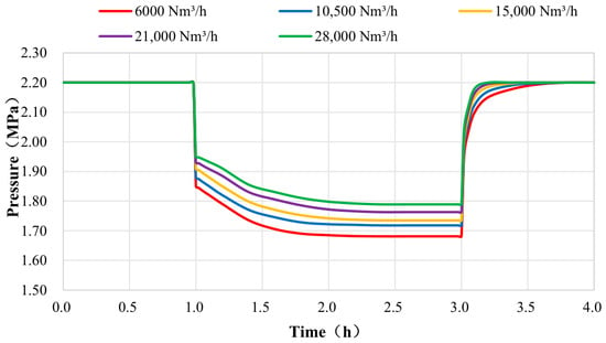
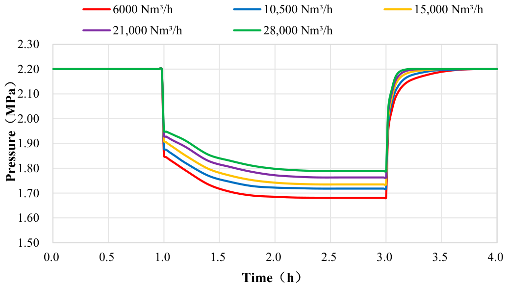
Figure 9 presents the pressure time-history curves for different inlet flow rates, and Table 12 summarizes the quantitative parameters. Figure 9 and Table 12 demonstrate the regulatory effect of different inlet flow rates (gas supply replenishment capacity) on the pressure evolution for a 150 mm leak.

Figure 9. Pressure evolution at leakage point under different inlet flow rates (150 mm hole, midpoint leakage, valve open).

Table 12. Pressure variation parameters under different inlet flow rates (150 mm hole, midpoint leakage, valve open).

Inlet Flow Rate (Nm3/h)	Minimum Steady-State Pressure (MPa)	Absolute Pressure Drop (MPa)	Relative Pressure Drop (%)	Pressure Variation Characteristics
6000	1.681	0.519	23.59	Severe insufficiency of gas supply replenishment; largest pressure drop
10,500	1.718	0.482	21.91	Relatively low replenishment; large pressure drop
15,000	1.735	0.465	21.14	Baseline case
21,000	1.763	0.437	19.86	Enhanced replenishment; pressure drop narrowed
28,000	1.789	0.411	18.68	High-flow replenishment; pressure relatively stable

As the inlet flow rate increases from 6000 to 28,000 Nm³/h, the minimum steady-state leak-point pressure rises from 1.681 to 1.789 MPa, while the relative pressure drop narrows from 23.59% to 18.68%, representing a reduction of 4.91 percentage points. With an increased inlet flow rate, the upstream gas source provides a stronger compensatory capacity against leakage losses, and the pressure equilibrium point is correspondingly elevated. It is noteworthy that even the maximum flow rate (28,000 Nm³/h, corresponding to a mass flow rate of 5.58 kg/s) is far smaller than the steady-state leakage rate for the 150 mm orifice (28.190 kg/s). The leakage volume still far exceeds the upstream replenishment capacity; therefore, a pressure drop in the pipeline network is inevitable, although the magnitude of the drop is somewhat alleviated as the flow rate increases.

During the plugging recovery stage, higher flow rates result in faster pressure recovery. Under high-flow conditions (21,000–28,000 Nm³/h), the pressure returns to its initial value within approximately 3.2 h. The above observations indicate that under low gas demand loads (6000 Nm³/h), the leakage-induced pressure drop is the largest, posing the highest risk of downstream gas supply interruption. Under peak loads (28,000 Nm³/h), although the pressure drop is smaller, the venting flow rate is higher, leading to a broader dispersion risk of combustion and explosion. Differentiated risk management and control strategies are therefore required for these two types of operating conditions.

3.4.2. Effect of Inlet Flow Rate on Leakage Rate Stability

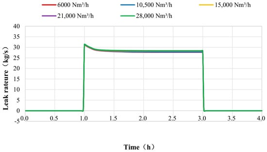
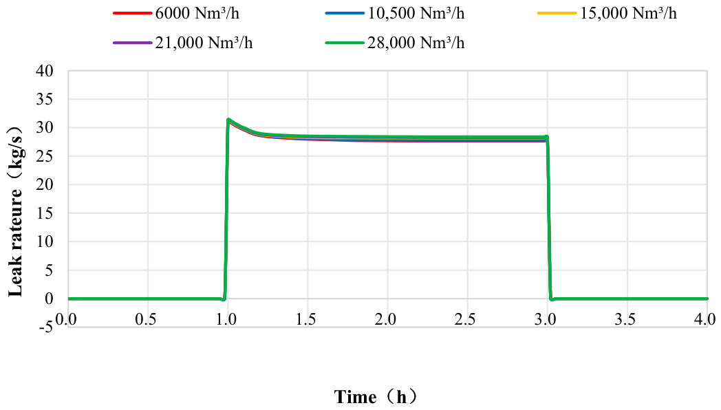
Figure 10 presents the leakage rate curves for different inlet flow rates, and Table 13 summarizes the quantitative parameters. Figure 10 and Table 13 demonstrate that the regulatory effect of inlet flow rate on the leakage rate is characterized by a “slight increase and enhanced stability” pattern.

Figure 10. Leakage rate evolution under different inlet flow rates (150 mm hole, midpoint leakage, valve open).

Table 13. Leakage rate parameters under different inlet flow rates (150 mm hole, midpoint leakage, valve open).

Inlet Flow Rate (Nm3/h)	Peak Leakage Rate (kg/s)	Steady-State Leakage Rate (kg/s)	Leakage Rate Reduction (%)	Rate Stability Characteristics
6000	31.058	27.652	10.97	Large rate decay after leakage; poor stability
10,500	31.124	27.964	10.15	Moderately large attenuation
15,000	31.247	28.190	9.78	Baseline case; moderate attenuation
21,000	31.338	28.516	9.01	Narrowed attenuation
28,000	31.416	28.843	8.19	Highest steady-state rate; smallest fluctuation

As the inlet flow rate increases from 6000 to 28,000 Nm³/h, the steady-state leakage rate rises from 27.652 to 28.843 kg/s, representing an increase of only 4.3% (+1.191 kg/s), which is far smaller than the increase in the flow rate itself (+367%). This is because the leakage rate for a 150 mm orifice far exceeds the inlet mass flow rate under any operating condition; the leakage rate is primarily governed by the orifice area and the leak-point pressure, while the upstream replenishment makes only a marginal contribution to the rate.

However, an increase in flow rate significantly improves rate stability: the rate reduction (i.e., the difference between peak and steady-state values) narrows from 10.97% (at 6000 Nm³/h) to 8.19% (at 28,000 Nm³/h). Under high-flow conditions, continuous upstream replenishment maintains the leak-point pressure at a relatively high level, resulting in smaller rate fluctuations and a smoother venting process.

Engineering implications: Under low-flow conditions, the pipeline pressure decays rapidly after leakage, and the rate decline is substantial, which may readily trigger low-pressure shutdown at the downstream end. Under high-flow conditions, the leakage rate remains persistently high with sustained venting intensity, leading to greater total release volumes. The actual dispersion distance and hazard zone extent would depend on local atmospheric conditions and require dedicated dispersion modeling. Valve-closure strategies should therefore be differentiated based on flow rate conditions, with more stringent closure logic (e.g., reduced detection delay and faster valve stroking) recommended during peak-load periods to mitigate the elevated release inventory.

3.5. Effect of Emergency Shut-Off Valve Operation on Leakage and Economic Losses

Taking the baseline case of a 150 mm orifice leak at the midpoint with an inlet flow rate of 15,000 Nm³/h, two scenarios—automatic closure of upstream and downstream emergency shut-off valves after leakage versus valves remaining fully open throughout—were compared to evaluate the control effectiveness of emergency valve closure from three dimensions: pressure, leakage rate, and cumulative economic losses.

3.5.1. Regulatory Effect of Shut-Off Valves on Leak-Point Pressure Evolution

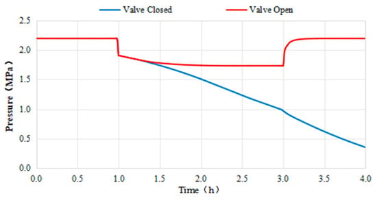
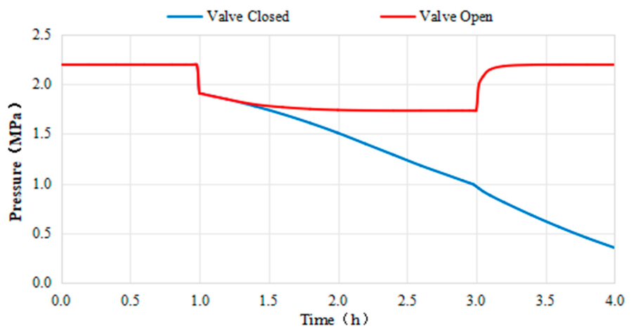
Figure 11 presents the evolution paths of leak-point pressure under both valve-closed and valve-open scenarios.

Figure 11. Pressure evolution at leakage point with and without emergency shutdown valve closure (150 mm hole, midpoint leakage, 15,000 Nm³/h).

In the valve-open scenario, immediately after leakage initiation, the pressure drops from 2.200 MPa to 1.910 MPa. Subsequently, owing to continuous upstream gas supply replenishment, the pressure gradually declines to 1.735 MPa and then forms a dynamic equilibrium (where the leakage venting flow rate equals the upstream replenishment flow rate). This steady-state pressure is maintained until plugging and recovery at 3 h.

In the valve-closed scenario, after the upstream and downstream shut-off valves are simultaneously closed, the isolated pipeline segment is completely cut off from the gas source. With no continuous gas replenishment inside the pipe, the pressure begins a one-way continuous decline from 1.910 MPa, dropping to 1.427 MPa at 1.5 h, 1.076 MPa at 2.0 h, 0.412 MPa at 3.0 h, and approaching 0.117 MPa at 4.0 h. If plugging repair is not implemented, the gas stored in the isolated pipeline segment will be completely vented until the pressure equilibrates with the ambient pressure.

Valve closure presents a double-edged effect: on the one hand, cutting off the gas supply replenishment prevents overall pressure instability in the pipeline network from propagating to upstream and downstream users, thereby avoiding a wider-scale gas supply interruption. On the other hand, the gas inside the isolated segment continues to vent, and the leak-point pressure has no recovery pathway, relying solely on the release of the gas inventory within the pipe segment [25]. Therefore, the essence of valve closure is to confine the leakage venting from the entire pipeline network to the gas inventory within the isolated segment, sacrificing local segment pressure in exchange for the overall stability of the main pipeline network.

3.5.2. Decisive Role of Shut-Off Valves in Leakage Rate Attenuation

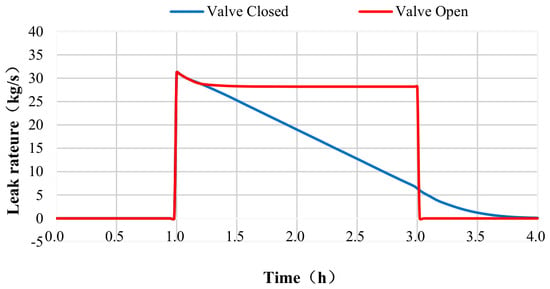
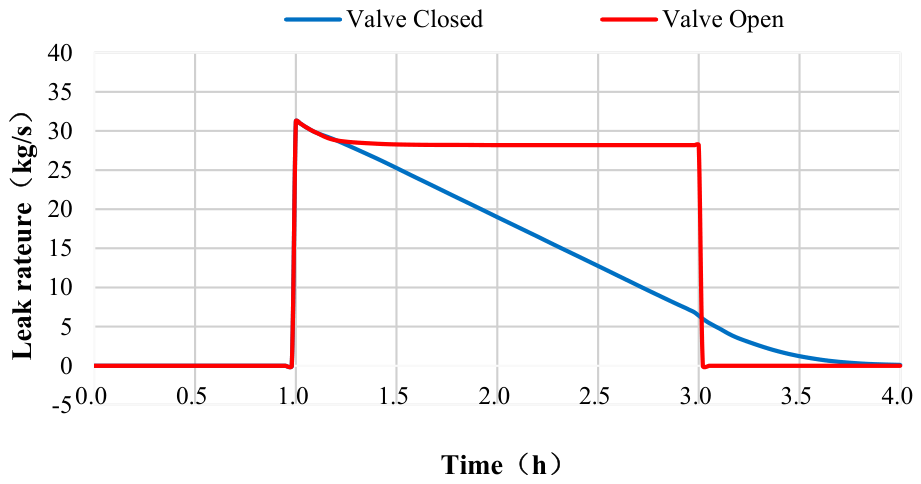
Figure 12 illustrates the control effect of shut-off valve closure on the leakage rate.

Figure 12. Leakage rate evolution with and without emergency shutdown valve closure (150 mm hole, midpoint leakage, 15,000 Nm³/h).

In the valve-open scenario, the leakage rate surges to a peak of 31.247 kg/s and then declines slightly to 28.190 kg/s, maintaining this high steady-state venting rate over an extended period. A continuous large-volume release of natural gas occurs during the 1–3 h period, with the leakage rate corresponding directly to the pressure equilibrium.

In the valve-closed scenario, after an initial surge, the leakage rate decays rapidly in an exponential manner, dropping to 21.683 kg/s (69.4% of the peak) at 1.5 h, 13.824 kg/s (44.2%) at 2.0 h, 7.319 kg/s (23.4%) at 2.5 h, 2.144 kg/s (6.9%) at 3.0 h, and approaching 0.015 kg/s (essentially depleted) at 4.0 h.

The core advantage of emergency valve closure is that it shortens the high-risk venting window from “indefinitely sustained (depending on repair time)” to “limited inventory (essentially depleted within approximately 2.5–3 h)”, greatly reducing the probability of secondary disasters such as explosions and toxic exposure, and creating relatively safe conditions for on-site repair operations.

The above analysis assumes simultaneous closure of upstream and downstream valves. To evaluate the effects of asynchronous valve closure, three scenarios were simulated: (1) the upstream valve closes 30 s in advance; (2) the downstream valve closes 30 s in advance; (3) single-valve failure. The results indicated that upstream-prioritized valve closure reduced the leakage rate by approximately 12% compared with simultaneous closure, with an additional 7.8% reduction in economic losses, representing the optimal strategy. By contrast, downstream-prioritized valve closure increased the leakage rate by around 7.5%, yielding the poorest performance. Under single-valve-failure conditions, the leakage rate was 25–40% higher than that for simultaneous valve closure. Thus, it is recommended that the valve-control logic prioritizes upstream-valve closure with a lead time of 5–30 s, and the time difference shall be controlled within ≤60 s. Regarding water-hammer risk, OLGA transient simulations revealed that the maximum water-hammer pressure increment induced by linear valve closure within 10 s ranged from 0.3 to 0.5 MPa, which is lower than the pipeline design pressure of 3.0 MPa and poses no threat to pipeline structural safety.

3.5.3. Economic Loss Reduction by Valve Closure for Different Hole Sizes

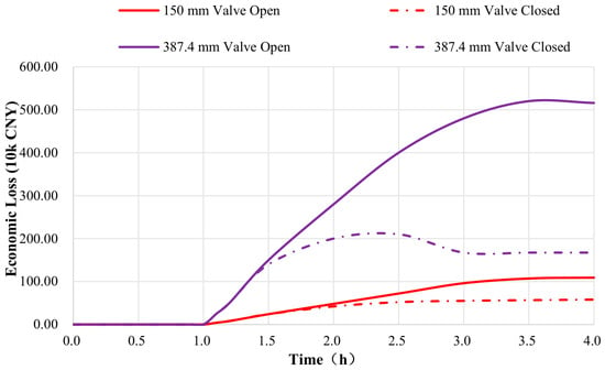
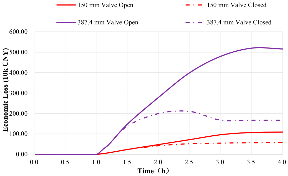
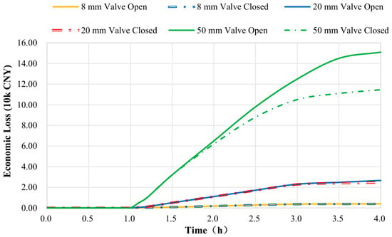
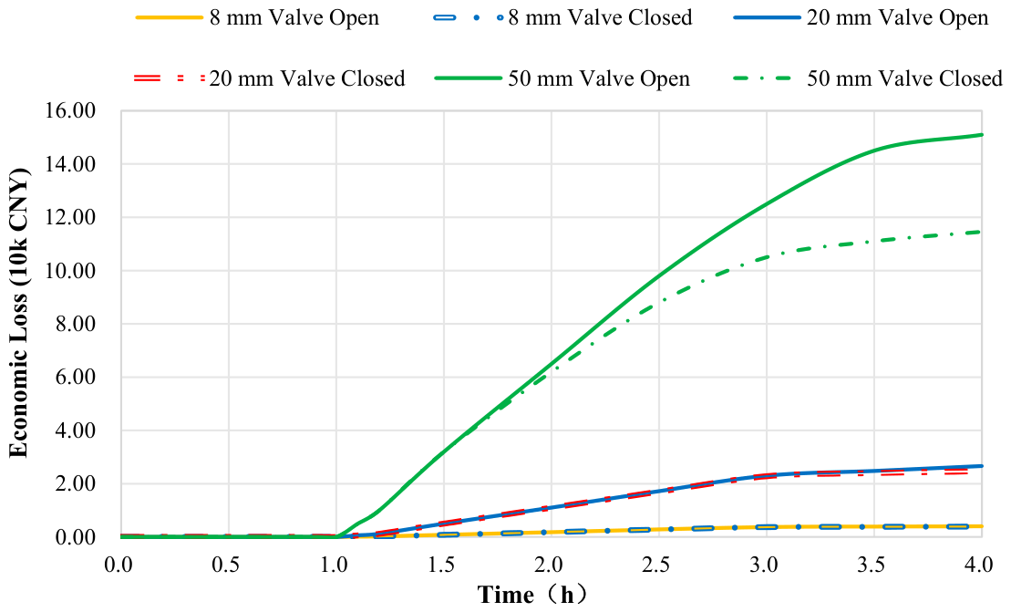
Figure 13, Figure 14 and Table 14 combine the natural gas market price of 3.59 CNY/Nm³ to calculate the cumulative economic losses over the 4 h simulation period for the five orifice diameters, quantitatively evaluating the loss-control effectiveness of shut-off valves under different leakage scales.

Figure 13. Comparison of cumulative economic losses before and after emergency shutdown valve closure for large leakage holes (150 mm and 387.4 mm in diameter).

Figure 14. Comparison of cumulative economic losses before and after emergency shutdown valve closure under small-diameter leakage conditions with hole diameters of 50 mm, 20 mm, and 8 mm.

Table 14. Economic benefits of emergency shutdown valve closure for different hole diameters (natural gas price: 3.59 CNY/Nm³).

Leak Orifice Diameter (mm)	Cumulative Economic Loss over 4 h with Valves Open (104 CNY)	Cumulative Economic Loss over 4 h with Valves Closed (104 CNY)	Loss Reduction Amount (104 CNY)	Loss-Control Rate (%)	Emergency Recommendation
8	0.37	0.36	0.01	2.7	Negligible loss control by valve closure; recommend on-stream sealing
20	2.30	2.16	0.14	6.1	Limited loss control; prioritize on-stream sealing
50	14.06	10.68	3.38	24.0	Valve closure significantly beneficial if repair >3 h
150	101.65	53.99	47.66	46.9	Immediate valve closure mandatory
387.4	515.92	167.37	348.55	67.6	Immediate valve closure mandatory; extremely significant loss-control effect

(1) Pinhole leak of 8 mm: The economic losses with and without valve closure are essentially identical (3700 vs. 3600 CNY), with a loss-control rate of only 2.7%. Considering indirect losses such as downstream customer service interruptions, valve closure is not economically justified; it is recommended to keep the valve open and perform on-stream sealing.

(2) Orifice of 20 mm: The loss-control rate is 6.1%, providing limited benefits. If the repair time is less than 4 h, valve closure may be omitted, and on-stream leak sealing should be prioritized.

(3) Medium-sized leak of 50 mm: The loss-control rate is 24.0%, reducing losses by 33 800 CNY over 4 h. When the repair duration exceeds 3 h, the cumulative loss curve under valve closure falls below that of the valve-open scenario. It is recommended to make the decision based on the repair progress.

(4) Large hole of 150 mm: The loss-control rate is 46.9%, reducing losses by 476,600 CNY over 4 h (from 1,016,500 CNY with valves open to 539,900 CNY with valves closed). Immediate valve closure is mandatory.

(5) Rupture of 387.4 mm: The loss-control rate is 67.6%, reducing losses by 3,485,500 CNY over 4 h (from 5,159,200 CNY with valves open to 1,673,700 CNY with valves closed), representing an extremely significant loss-control effect. Under valve closure, the gas inventory in the isolated segment for large-hole and rupture scenarios is essentially depleted within approximately 2.5 h, after which economic losses cease to grow, whereas losses under the valve-open scenario continue to rise linearly.

In summary, the graded emergency response strategy is as follows: for ≤20 mm leaks, perform on-stream sealing without valve closure; for 50 mm leaks, decide based on repair duration (close valves if repair >3 h); for ≥150 mm leaks, immediate interlocking valve closure is mandatory.

It should be emphasized that the above-mentioned graded valve-closure suggestions are mainly based on two dimensions: hydraulic feasibility (pipeline pressure maintenance capacity) and direct economic losses of natural gas. In practical emergency decision-making, the following risk factors must also be comprehensively considered:

(1) Fire and explosion risk: If the leaked natural gas encounters an ignition source, jet fire or vapor cloud explosion may occur, and its hazard range depends on the leakage rate, meteorological conditions and surrounding environment.

(2) Ignition probability: Closely related to leakage duration, leakage rate and the distribution of surrounding ignition sources.

(3) Population exposure: The population density around the leakage point determines the potential casualty risk level.

(4) Social impacts of gas supply interruption: Large-scale gas outages caused by upstream leakage may lead to secondary social problems.

(5) Safety of maintenance personnel: Pressurized leak-stopping operations inherently carry risks such as high-pressure gas jetting and fire.

(6) Uncertainty in leakage-size identification: It is difficult to accurately measure the leakage orifice diameter in real-world emergencies, and comprehensive judgment should be made based on measurable parameters such as pressure drop rate.

Therefore, a complete emergency valve-closure decision shall be comprehensively judged on the basis of the dynamic leakage characteristics obtained in this study, combined with CFD dispersion simulation, consequence assessment and real-time on-site monitoring data. The recommendations presented in this study should be regarded as one of the references for emergency decision-making rather than the sole criterion.

4. Conclusions

Taking the urban JS high-pressure gas pipeline as the engineering carrier, this study established a time-varying leakage numerical model based on the OLGA full-dynamic multiphase flow simulation software. The main conclusions are:

(1) A standard four-stage coupled evolution pattern exists throughout the entire leakage process. In the absence of emergency intervention, the leak-point pressure sequentially undergoes four stages: “steady-state operation → instantaneous sharp drop → gradual decay to dynamic equilibrium → rapid recovery after plugging.” The leakage rate exhibits a corresponding four-stage response: “zero leakage → instantaneous peak surge → exponential decay to steady-state venting → instantaneous return to zero.” Pressure and leakage rate are positively and strongly coupled. After plugging, the pipeline pressure can recover to its initial value within 1 h, verifying the effectiveness of the dynamic simulation model in characterizing gas supply replenishment and pressure wave propagation.

(2) The leak orifice diameter is an exponential-level controlling factor for accident magnitude. An 8 mm pinhole leak causes virtually no disturbance to pipeline pressure (relative pressure drop of only 0.055%), and from the perspective of hydraulic acceptability, it qualifies for on-stream sealing; for a 20 mm orifice, the pressure drop is 0.76%, and the main transmission function remains unaffected; for a 50 mm orifice, the pressure drop reaches 6.52%, requiring attention to downstream gas supply; for the 150 mm large hole and 387.4 mm rupture cases, the steady-state pressure drops reach 21.14% and 76.32%, respectively, with peak leakage rates of 31.247 kg/s and 187.536 kg/s, resulting in a sharp increase in release volume. A level-1 emergency response must be activated. Although increasing the orifice diameter raises the leakage rate, the rate increase is less than the theoretical value based on area ratio due to the “pressure-drop self-feedback” effect. It should be particularly noted that the final decision on on-stream repair must comprehensively consider mechanical safety factors such as defect geometry, remaining wall thickness, local stress, and repair techniques; the conclusions of this study are applicable only to the hydraulic feasibility assessment stage.

(3) Leakage location determines the type of risk; upstream pipeline sections dominate the risk of gas supply interruption, while downstream sections dominate the risk of sustained combustion and explosion. A leak at the upstream location of 1.5 km causes a pressure drop of 23.62% across the entire pipeline, with the lowest steady-state rate (26.847 kg/s). In contrast, a leak at the downstream location of 9.0 km causes virtually no pressure disturbance (pressure drop of 1.68%) but exhibits the highest steady-state leakage rate (30.578 kg/s) with minimal rate attenuation (only 1.53%). It is recommended that intrinsic safety design and construction protection be strengthened in upstream sections, while the layout of shut-off valves in downstream sections be optimized to improve shutdown response speed.

(4) Inlet flow rate regulates the pressure equilibrium point through upstream replenishment capacity but has a relatively minor effect on the leakage rate. When the inlet flow rate increases from 6000 to 28,000 Nm³/h, the steady-state pressure for a 150 mm orifice leak rises from 1.681 to 1.789 MPa (pressure drop narrowed by 4.91 percentage points), while the steady-state rate increases by only 4.3%. Under high-flow conditions, the rate fluctuation is smaller, and the venting process is more stable; however, the absolute release volume and sustained release intensity are greater, leading to increased potential severity of the accident.

(5) Emergency shut-off valves exhibit significant loss-control effectiveness for large-diameter leaks, and a graded valve-closure strategy should be implemented. Valve closure cuts off the gas source, converting “continuous venting from the entire pipeline network” into “limited release of the gas inventory within the isolated segment,” resulting in an exponential decay of the leakage rate. For the 150 mm and 387.4 mm cases, cumulative economic losses over 4 h are reduced by 46.9% and 67.6%, respectively (corresponding to savings of 476,600 and 3,485,500 CNY). However, for 8 mm and 20 mm small holes, the loss-control rate is less than 6%, and valve closure may cause indirect losses due to downstream customer service interruptions. It is therefore recommended to keep the valves open and perform on-stream sealing. For 50 mm medium-sized leaks, the decision should be based on repair duration (close valves if repair time exceeds 3 h). For leaks ≥150 mm, immediate interlocking valve closure is mandatory.

The OLGA-based dynamic leakage simulation model for urban high-pressure gas pipelines developed in this study is capable of fully reproducing the entire time-varying behavior of leakage initiation, steady-state venting, and plugging repair. It overcomes the limitation of traditional steady-state analytical models, which cannot characterize the dynamic processes of gas supply replenishment and valve-actuated operations. The simulation data provide theoretical support and quantitative reference for leakage risk classification, interlocking logic optimization of shut-off valves, and the formulation of on-site emergency response plans for urban high-pressure gas pipeline networks.

References

- Han, M. Analysis on urban gas pipeline engineering construction and equipment safety management. China Equip. Eng. 2025, 14, 50–52. [Google Scholar]
- Kim, J.H.; Ko, B.S.; Yang, J.M.; Ko, S.-W.; Ko, J.W. Consequence analysis for release scenario of buried high pressure natural gas pipeline. Korean Chem. Eng. Res. 2014, 52, 306–312. [Google Scholar]
- Poursanidis, K.; Sharanik, J.; Hadjistassou, C. World’s largest natural gas leak from nord stream pipeline estimated at 478,000 tonnes. iScience 2024, 27, 108772. [Google Scholar] [CrossRef] [Scilit]
- He, L.M.; Wang, L. Progress in gas dispersion law and gas-liquid separation technology during high-pressure natural gas pipeline rupture. Pet. Ind. Tech. Superv. 2005, 5, 89–93. [Google Scholar]
- Yan, M.Q.; Li, J.; Guan, Y.W. Rupture leakage model for a natural gas pipeline. J. Pipeline Syst. Eng. Pract. 2023, 14, 04022060. [Google Scholar] [CrossRef] [Scilit]
- Jo, Y.D.; Ahn, B.J. A simple model for the release rate of hazardous gas from a hole on high-pressure pipelines. J. Hazard. Mater. 2003, 97, 31–46. [Google Scholar] [CrossRef] [Scilit]
- Montiel, H.; Vílchez, J.A.; Casal, J.; Arnaldos, J. Mathematical modelling of accidental gas releases. J. Hazard. Mater. 1998, 59, 211–233. [Google Scholar] [CrossRef] [Scilit]
- Huo, C.Y.; Dong, Y.H.; Yu, D.T.; Gao, H.L.; Zhou, J.E.; Feng, Y.R. Research on calculation method of gas leakage rate for long-distance pipeline. Acta Pet. Sin. 2004, 25, 101–105. [Google Scholar] [CrossRef]
- Feng, W.X.; Wang, Z.Q.; Cheng, W.Y. Comparative analysis of small-hole and large-hole leakage models for high-pressure gas pipelines. Saf. Environ. Eng. 2009, 16, 108–110. [Google Scholar]
- Wang, D.Q.; Huo, C.Y.; Gao, H.L. Simplified calculation method for gas leakage rate of long-distance pipeline. Nat. Gas Ind. 2008, 28, 116–118. [Google Scholar]
- Dong, Y.H.; Zhou, J.E.; Gao, H.L.; Huo, C.Y.; Feng, Y.R. Calculation of steady-state gas leakage rate for long-distance pipeline. Oil Gas Storage Transp. 2002, 21, 11–15. [Google Scholar]
- Dutkiewicz, M.; Dalyak, T.; Shatskyi, I.; Venhrynyuk, T.; Velychkovych, A. Stress Analysis in Damaged Pipeline with Composite Coating. Appl. Sci. 2021, 11, 10676. [Google Scholar] [CrossRef] [Scilit]
- Liu, Z.; Chen, Y.; Wu, Q. Numerical simulation of the mechanical interaction between a mobile lift chain and a main gas pipeline during repair operations. Eng. Fail. Anal. 2023, 148, 107189. [Google Scholar]
- Wang, J.; Zhao, H.; Sun, L. Analytical model for the interaction of an oil pipeline with an overpass support in mountainous terrain. Int. J. Press. Vessels Pip. 2024, 207, 105132. [Google Scholar]
- Yang, X.; Zhang, L.; Ren, S. Girth weld defect assessment and repair decision framework for high-strength pipeline steels. Nat. Gas Ind. 2023, 43, 112–121. [Google Scholar]
- Fu, J.M.; Zhao, Z.Y.; Chen, G.M.; Luo, H.J.; Zhang, B.P.; Zhang, B.L.; Ye, C.; Zhu, Y. Influences of liquid pipeline flow and pressure on small-hole leakage rate. Acta Pet. Sin. 2016, 37, 257–265. [Google Scholar] [CrossRef]
- Ebrahimi-Moghadam, A.; Farzaneh-Gord, M.; Deymi-Dashtebayaz, M. Correlations for estimating natural gas leakage from above-ground and buried urban distribution pipelines. J. Nat. Gas Sci. Eng. 2016, 34, 185–196. [Google Scholar] [CrossRef] [Scilit]
- Ji, H.; Guo, J.; Zhang, G.; Yang, K.; Jiang, J.; Wang, Y.; Xing, Z.; Bi, H. Multi-Factor Coupling Analysis of Porous Leakage in Underwater Gas Pipelines. Processes 2023, 11, 1259. [Google Scholar] [CrossRef] [Scilit]
- Jiang, H.Y.; Xie, Z.Y.; Li, Y.L.; Chi, M. Leakage and diffusion of high-pressure gas pipeline in soil and atmosphere: Experimental and numerical study. Energy Sources Part A Recovery Util. Environ. Eff. 2023, 45, 10827–10842. [Google Scholar] [CrossRef] [Scilit]
- Fu, J.M.; Zhang, B.L.; Chen, G.M.; Zheng, X.; Ye, C.; Guo, C.; Zhu, Y. Hole-leakage rate model of whole process based on intervention of liquid level control system. CIESC J. 2017, 68, 473–480. [Google Scholar]
- de Almeida, J.C.; Sardá, A.P.; de Oliveira, H.S.F. Volume of natural gas released into the atmosphere in leakage situations-review and analysis. Int. J. Adv. Eng. Res. Sci. 2022, 9, 173–177. [Google Scholar] [CrossRef] [Scilit]
- API (American Petroleum Institute). API Recommended Practice 581: Risk-Based Inspection Methodology, 3rd ed.; API Publishing Services: Washington, DC, USA, 2020. [Google Scholar]
- GB/T 34346-2017; Guidelines for Risk Based Safety Hazard Classification of Oil and Gas Pipelines. Standardization Administration of China: Beijing, China, 2017.
- Aliyev, I.G.; Karimov, E. Invariant-based analysis of transient gas flow and optimal valve spacing in pipelines. Math. Comput. Appl. 2026, 31, 139. [Google Scholar] [CrossRef] [Scilit]
- Ma, X.Y.; Ouyang, X.; Zhu, J.L.; Chen, J.W.; Liu, L.Q.; Yang, T.; Song, G.C. Adaptability evaluation of the software for transient process simulation of supercritical CO2 pipelines. Oil Gas Storage Transp. 2024, 43, 590–599. [Google Scholar]
Disclaimer/Publisher’s Note: The statements, opinions and data contained in all publications are solely those of the individual author(s) and contributor(s) and not of MDPI and/or the editor(s). MDPI and/or the editor(s) disclaim responsibility for any injury to people or property resulting from any ideas, methods, instructions or products referred to in the content. |
© 2026 by the authors. Licensee MDPI, Basel, Switzerland. This article is an open access article distributed under the terms and conditions of the Creative Commons Attribution (CC BY) license.