


Abstract
In high-voltage cable sheaths, incipient weak faults, such as jacket-damage grounding and high-resistance core–sheath breakdown, release little energy, rarely trigger protection, and can evolve into permanent faults. This study examines whether the topology-induced joint structure of multichannel sheath currents can support fault detection without fault samples. A Mahalanobis-distance-based method is formulated for the three-phase sheath circulating currents measured at a single cross-bonding box. An induction–leakage analysis relates the healthy joint structure to the bonding topology and shows how weak faults disturb it. A normalized pointwise Mahalanobis distance is combined with a threshold calibrated on separate healthy data and a K-consecutive-sample rule; the method requires no signal decomposition, and its per-sample cost is constant. On a PSCAD model of a 110 kV cross-bonded system, all 52 development fault cases are detected with confirmation delays below 6 ms; an independent sixteen-record healthy test is false-alarm-free after an envelope recalibration; boundary-grade faults under joint non-ideal conditions retain nine-fold margins; and per-line calibration extends the criterion to asymmetric and longer geometries. A twenty-seed Monte Carlo campaign shows zero noisy false alarms at all tested signal-to-noise ratios, the observable fault range being set by the disturbance-to-noise energy ratio of the acquisition chain.
1. Introduction
The secure and stable operation of power systems underpins the normal functioning of modern society, and the reliability of cable networks is particularly critical. With the continuous growth of urban load density, large-capacity cross-linked polyethylene (XLPE) single-core cables have become the backbone transmission equipment of urban power grids, and accordingly, their life-cycle management and condition monitoring have received sustained attention [1]. However, for power cables buried underground over long periods, mechanical damage combined with water ingress drives progressive insulation degradation that develops into grounding faults and outages, as demonstrated experimentally on damaged low-voltage cables [2]. If incipient faults could be detected and handled before they evolve into permanent faults, cable operation and maintenance could shift from post-fault repair to pre-fault warning, effectively preventing fault escalation. Research on incipient cable fault detection is therefore of substantial engineering significance.
Regarding the definition of incipient cable faults, existing studies have offered characterizations from different perspectives. Reference [3] classifies incipient faults as recoverable arc faults, appearing in half-cycle and multi-cycle forms lasting about a quarter cycle and one to four cycles, respectively. Reference [4] characterizes incipient faults in underground distribution cables as intermittent, self-clearing events of sub-cycle or multi-cycle duration. Reference [5] surveys cable aging mechanisms and diagnostics, identifying gradual insulation aging and localized deterioration such as water treeing as the physical origin of such faults. Reference [6], reviewing high-impedance faults, characterizes grounding through high-resistance paths by its low-magnitude, arc-accompanied currents, which fall within the weak fault regime addressed in this paper. Reference [7] further treats incipient faults as events with inconspicuous signatures accompanied by self-clearing arcs and additionally addresses their location.
In terms of the energy released at the fault instant, recoverable arc faults, though short-lived, involve a violent release process, and the resulting high temperature and sparks threaten to ignite nearby combustibles. The focus of this paper is incipient weak faults that carry even less energy than do recoverable arc faults and sit further upstream in the fault evolution chain, namely, the sheath grounding fault and the high-resistance core–sheath short-circuit fault. Their transient responses in the phase currents and phase voltages are even less pronounced, placing higher demands on detection sensitivity. Conventional periodic inspection and preventive testing cannot meet real-time requirements, and incipient fault detection methods based on advanced signal processing and data analysis have become a research focus.
Existing studies on incipient fault detection can be grouped into signal processing, machine learning, and neural network approaches. Reference [8] identified incipient faults by combining numerical modeling with statistical change detection applied to voltage and current measurements, an early statistical treatment that resonates with the criterion philosophy of this paper. Reference [9] detected series AC arc faults from energy-profile features of voltage waveforms alone while avoiding false alarms. Reference [10] used the ratio of the measured to the expected sheath current as a criterion, realizing online monitoring and diagnosis of HV cable faults. Reference [11] achieved online tracking of the relative dielectric loss of cross-bonded cables using sheath currents. Reference [12] detected and located sheath defects in cross-bonded systems based on sheath current ratio features. Reference [13] realized fault location for cross-bonded HV cable systems by monitoring the sheath currents. Reference [14] diagnosed reverse-connection defects in the cross-bonded grounding system of high-voltage cables based on ARO–SVM. Reference [15] established a model for assessing the magnitude and distribution of sheath currents in medium- and high-voltage cable lines. Reference [16] demonstrated the feasibility of detecting sheath faults by monitoring the sheath-to-ground currents at the ends of cross-bonding sections. Reference [17] realized online fault location using sheath currents on a 38 km cross-bonded underground transmission line. Reference [18] achieved fault location for cross-bonded cables by exploiting the reactive-power characteristics of the core–sheath transition resistance. These criterion-based methods share a common assumption. A scalar feature or an inter-channel ratio departs measurably from its nominal value once a defect is present. This holds for permanent defects that shift the operating point, but it provides no principled false-alarm control when the healthy background itself fluctuates, and the incipient grades considered here perturb such scalar features by far less than the natural variation of normal operation. On the learning side, Reference [19] embedded time–frequency transforms into an attention-based deep learning model to identify incipient faults in power distribution systems. Reference [20] combined the S-transform and the Hilbert transform to extract incipient fault features, followed by least-squares support vector machine identification. Reference [21] extracted seven features from abnormal voltage waveforms recorded by power quality monitors and achieved classification through feature selection and a particle-swarm-optimized support vector machine. Reference [22] stacked restricted Boltzmann machines into a deep belief network and identified cable faults with a Softmax classifier. Reference [23] extracted three features (time delay, peak voltage, and time–frequency phase angle difference) from the fault waveform and its reflection and fed them into a general regression neural network for fault identification. Reference [24] detected series AC arc faults directly from raw current waveforms with a convolutional neural network (ArcNet). These classifier-based methods presuppose labeled fault samples that cover the deployment conditions; for incipient faults, whose recorded instances are scarce and rarely representative of unseen severities, this assumption is difficult to satisfy, and the resulting decision boundaries resist physical interpretation. For sheath current signals specifically, Reference [25] identified incipient faults of 10 kV single-core cables from a single-channel sheath current with a convolutional neural network. Reference [26] fused sheath current features with a denoising variational autoencoder and ensemble learning to identify incipient faults of 10 kV cables. Sheath currents have also supported a broader family of monitoring applications. Reference [27] detected and localized connection defects in cable screens from screen-current measurements. Reference [28] detected two-sheath-loop short-circuit defects with sheath current phasors. Reference [29] combined the sheath current with the resistive current and the dielectric loss factor for integrated insulation monitoring of cross-bonded cables, and Reference [30] identified cable circuits online via deep embedded clustering of sheath current time series. On the learning side, Reference [31] diagnosed sheath grounding-system faults with an LSTM network over amplitude-ratio and phase-difference features, and Reference [32] combined WOA–CEEMDAN decomposition with a TCN–BiLSTM network for incipient cable fault identification. Reference [33] employed optimal variational mode decomposition (OVMD) with the impulse factor and cosine similarity to select feature modes, constructed a criterion from the ratio of segmented Teager–Kaiser energy operator (TKEO) derivatives, and detected incipient faults on the sheath grounding-lead current of 10 kV single-end-grounded cables, representing the state of the art in this direction. These decomposition-plus-learning pipelines inherit the constraints of both ingredients. The decomposition stage presupposes that the fault signature is separable from the power-frequency background, the classifier stage again requires fault examples, and the criteria remain single-channel, so the cross-channel structure specific to cross-bonded systems is left unused. Beyond fault detection, data-driven modeling of normal operating behavior is advancing rapidly across power-system monitoring at large; pre-trained large models with retrieval-augmented generation have recently been applied to distributed photovoltaic power forecasting [34]. Such large-model pipelines, however, presuppose data and computing resources far beyond what sheath-current monitoring terminals provide, which further motivates the lightweight statistical route pursued here.
Summarizing the existing research, three deficiencies remain. First, most methods construct features from phase currents and phase voltages, in which the fault response of incipient weak faults is feeble; detection performance is poor and susceptible to noise [8,9,19,20,21,22,24]. Second, the criteria or features of sheath-current-based methods are mostly taken from single-channel signals or inter-channel ratios [10,11,12,13,14,15,16,17,18,25,26,27]; the three-phase circulating currents have not been modeled structurally as a joint distribution, leaving the spatial correlation among the three-phase circulating currents in cross-bonded systems unexploited. Third, time–frequency decomposition methods are inherently limited in separating weak faults at the power frequency, require substantially more decomposition levels under strong noise [32,33] with a marked computational burden, and their thresholds are mostly set empirically, leaving the false-alarm rate unassessable.
To address these deficiencies, this study examines whether the topology-induced joint structure of multichannel sheath currents can support incipient weak fault detection without fault samples. In a cross-bonded grounding system, the three-phase sheath circulating currents at one cross-bonding box are jointly determined by the bonding topology and the line geometry. They exhibit a structured healthy distribution, while a weak fault can disturb the inter-channel relationship. Accordingly, healthy operating data are used to estimate a baseline mean and covariance, and a normalized pointwise Mahalanobis distance is combined with a threshold calibrated on a separate healthy set and a consecutive-crossing rule. Evidence is evaluated with a PSCAD simulation model of a 110 kV cross-bonded cable system. The study, therefore, provides simulation-based feasibility and sensitivity evidence rather than field validation. A comparison with the single-channel segmented TKEO method is retained as a scoped transferability check. The main contributions of this paper are as follows:
- (1)
- An analytical induction–leakage model of the three-phase sheath circulating currents of cross-bonded cables is established. Starting from the symmetry of the bonding topology, the stability of the healthy joint structure of the circulating currents and its disruption mechanism under weak faults are elucidated, providing the physical basis for multi-channel joint detection;
- (2)
- A weak fault detection index based on the healthy-baseline Mahalanobis distance is proposed. Its covariance whitening mechanism accommodates amplitude differences and channel correlations in the three-phase circulating currents. The method requires neither signal decomposition nor fault samples, and its per-sample complexity is constant, supporting future implementation on online monitoring terminals, subject to hardware and field-data validation;
- (3)
- A threshold setting method based on an independent healthy calibration set and a consecutive-crossing criterion are proposed, making the false-alarm rate explicitly controllable and overcoming the unassessable false-alarm rate of empirical threshold methods.
2. Incipient Weak Fault Characteristics of Cross-Bonded Cables
2.1. Cross-Bonded Grounding System
In high-voltage single-core cable lines, the alternating magnetic field of the conductor current induces a longitudinal electromotive force (EMF) on the metallic sheath (Figure 1), and the induced sheath voltage accumulates with cable length. For lines longer than 1000 m, sheath cross-bonding is common engineering practice, in which the line is divided into several major sections, each equally divided into three minor sections; insulated joints are installed between adjacent minor sections, and the sheaths are transposed at the cross-bonding joints so that each sheath circuit successively passes through the corresponding minor sections of phases A, B, and C; the sheaths at both ends of a major section are solidly grounded. Ideally, the superposition of the EMFs induced on the three minor sections is approximately zero, and the sheath circulating current is significantly suppressed.
Figure 1.
Cross-section of a 110 kV single-core XLPE cable, drawn to scale, with the outer radii of the conductor, insulation, sheath, and jacket denoted as rC, rI, rS, and rJ, respectively.
The subject of this study is one complete cross-bonded major section, as shown in Figure 2. At the cross-bonding box, the three sheath circuits are transposed through three connecting links, and each link carries the circulating current of exactly one sheath loop; the three sheath circulating currents, denoted , , and , can therefore be measured separately inside the box, with the subscripts corresponding to the joint numbers J1–J3 in Figure 2. This measuring point is centralized, non-intrusive, and convenient for retrofitting clamp-type current sensors on the links, making it a natural entry point for online monitoring.
Figure 2.
Cross-bonded cable system under study. The three sheath circulating currents J1–J3 are measured on the transposition links inside the first cross-bonding box (joints J1–J3).
2.2. Mechanism of Incipient Weak Faults
During long-term operation, cables are subject to soil chemical corrosion, moisture ingress, and mechanical stress, and their insulation gradually degrades. In cross-bonded systems, incipient weak faults mainly appear in two forms. The first is the sheath grounding fault (SGF), in which the metallic sheath, after local damage to the outer jacket, forms an unintended grounding path to earth through a transition resistance, creating an additional circulating loop under multi-point sheath grounding. The second is the high-resistance core–sheath fault (CSF), in which local degradation of the main insulation forms a weak channel, and the core leaks current to the sheath through a high-resistance path. In their early stages, both fault types involve large transition resistances and feeble fault currents that leave the core electrical quantities nearly unaffected, yet both alter the impedance distribution and boundary conditions of the sheath system, constituting typical incipient weak faults. If left untreated, the transition resistance continues to decrease as degradation proceeds, evolving successively into occasional recoverable arc faults, frequent intermittent arc faults, and ultimately, a permanent fault (Figure 3).
Figure 3.
Schematic evolution of the cable state over the service life, with the incipient-fault-prone stage (5–10 years) as the focus of this work; the time axis is nonlinearly compressed for readability.
It should be noted that the weak faults studied here sit at the very front of the fault evolution chain, and their sheath circulating current responses may amount to only a small percentage of the normal circulating current. The detection method must therefore be sufficiently sensitive to weak changes while remaining sufficiently robust to normal disturbances such as load fluctuations.
2.3. Analysis of the Three-Phase Sheath Circulating Current Signals
The sheath circulating current measured at the cross-bonding box consists of two components, i.e., an induced component generated on the sheath circuits by electromagnetic coupling of the three-phase core currents and a leakage component flowing from the core to the sheath through the equivalent impedance of the main insulation. The two components are modeled separately below, and the joint structural property of the healthy three-phase circulating currents is then derived.
The three sheath circulating currents are the only inputs measured in this paper; neither phase voltages nor phase currents are used, for two reasons. Regarding signal content, both fault types listed in Section 2.2 reconfigure the sheath circuit directly, either by adding a grounding branch to a sheath loop or by injecting core current into the sheath through the degraded insulation, so the sheath circulating currents carry the fault disturbance, even though they are themselves small quantities; the same incipient grades only perturb the phase voltages and phase currents through the negligible change of the line series impedance, a relative change that is not expected to be resolvable by conventional instrument transformers. Regarding instrumentation, the cross-bonding box is a non-intrusive low-voltage measurement point at which clamp current transformers on the transposition links suffice; measuring the phase voltages would require potential transformers that are not installed at the box, adding cost without providing usable signal content at these fault grades.
- (1)
- Calculation of the Induced Sheath Component
When the three-phase currents , , and flow through the cores of the single-core cables, they generate alternating magnetic fields in the surrounding space. Taking any phase core as an example, the magnetic field strength at a distance x from the cable axis is
where I is the core current of that phase, and x is the distance from the cable center.
The magnetic flux density is
where μ is the magnetic permeability of the medium.
Taking a radial element of width dx, the magnetic flux through the rectangle it forms (with a unit axial length) is dφ = B(x)dx. With the notation shown in Figure 1, the sheath inner surface lies at the insulation outer radius . For the same phase, the flux linkage with the sheath is the integral of the flux between the conductor outer surface () and the sheath inner surface, i.e., the per-unit-length flux linkage
Hence, the per-unit-length self-inductance between the core and the sheath of the same phase and the corresponding induced EMF are, respectively,
where I = I0 cos(ωt + φ0), with I0 as the current amplitude, ω as the power angular frequency, and φ0 as the phase angle.
Similarly, the core currents of the adjacent phases induce EMFs on this sheath through mutual coupling. Let (j, k ∈ {A, B, C}, j ≠ k) denote the distance between the axis of the adjacent-phase core and this sheath; the per-unit-length mutual inductance and induced EMF are then
where Ij0 and φj are the amplitude and phase angle of the phase-j core current, respectively. The mutual coupling between sheaths contributes little to the induced voltage and is neglected for simplicity; the direct induction of the core currents on the sheath is considered as the dominant effect.
- (2)
- Synthesis of the Loop EMF Under Cross-Bonding
Unlike a single-end-grounded system, each sheath circuit in a cross-bonded system runs through three minor sections and is coaxial with a different phase core in each of them. Let the i-th sheath circuit (i = 1, 2, 3) be coaxial with the cables of phases σi(1), σi(2), and σi(3) in the three minor sections (σi is the transposition permutation), whose lengths are l1, l2, and l3. The total induced EMF of the circuit is the accumulation of the per-unit-length EMFs over the section lengths:
where eσi(m) is the per-unit-length resultant induced EMF at the position of this circuit in the m-th minor section, obtained by superposing the self- and mutual-inductance components of Equations (5) and (6).
When the three minor sections are of equal length (l1 = l2 = l3) and the three-phase currents are symmetric, the induced EMF phasors of the three minor sections differ successively by 120°, and their superposition is approximately zero, suppressing the sheath circulating current to a very low level. In practical lines, however, the minor-section lengths are not strictly equal, the layout geometry is not perfectly symmetric, and the three-phase load is unbalanced; the residual EMF in the loop is nonzero, and the circulating current of the i-th circuit is
where Zs,i is the impedance of the i-th sheath circuit itself, and Zg1 and Zg2 are the grounding impedances of the grounding devices at the two ends of the major section. The phasor cancellation underlying Equations (7) and (8) is illustrated in Figure 4, where under healthy conditions, the induced EMFs of the three minor sections traversed by a sheath loop are equal in magnitude and mutually displaced by 120°, so their phasor sum closes, and the circulating current is suppressed (Figure 4a); a weak fault perturbs the EMF of the faulted section only, the closure is broken, and the residual EMF drives an additional circulating current, since the three loops are perturbed in different sections, ΔJ1 ≠ ΔJ2 ≠ ΔJ3 (Figure 4b, Equation (12)).
Figure 4.
Phasor interpretation of the cross-bonding cancellation mechanism: (a) healthy conditions, the phasor sum of the three sectional EMFs closes; (b) weak-fault conditions, the closure is broken and a residual EMF appears; the dashed phasor marks the pre-fault EMF of the faulted section.
- (3)
- Leakage Component and Circulating Current Synthesis
The main insulation between the core and the sheath can be represented by an equivalent impedance . With V denoting the voltage difference between the core and the sheath, the leakage current is
After injection into the sheath, the leakage current divides into ILL and ILR, according to the sheath impedances ZSL and ZSR on either side of the injection point, and returns through the groundings at the two ends; in the equivalent circuit shown in Figure 5, IC and ZCX denote the core current and the core longitudinal impedance, respectively, and Rg the terminal grounding resistance, while the left-hand leakage share flows toward the measuring side. The i-th sheath circulating current measured at the cross-bonding box is the instantaneous superposition of the induced and leakage components (Figure 5):
Figure 5.
Equivalent circuit of the core–insulation–sheath path of one phase.
- (4)
- Healthy Joint Structure and Its Disruption
Equations (7) and (8) show that the amplitudes and phases of the healthy three-phase circulating currents are jointly determined by the transposition topology σi, the minor-section lengths, the layout geometry, and the system impedances. For a given line, these parameters remain unchanged during normal operation, so the three-phase circulating currents satisfy a stable joint symmetric structure:
Moreover, load-level variations scale the three-phase circulating currents approximately proportionally, leaving the shape of the joint structure unchanged. This stability, anchored by the physical topology, is the physical basis on which the healthy-baseline statistical model introduced later can be learned and extrapolated.
When an incipient weak fault occurs, let denote the fault-induced change in the i-th phase circulating current; the post-fault current is then
where Jih(t) is the healthy circulating current. For the SGF, the additional grounding path alters the boundary conditions and impedance distribution of the faulted sheath circuit; for the CSF, the leakage current is injected directly into the faulted-phase sheath. In both cases, owing to the asymmetry of the cross-bonded coupling, ΔJ1, ΔJ2, and ΔJ3 are in general unequal, and the joint symmetric structure of Equation (11) is disrupted.
The key point is that, under a weak fault, the single-channel amplitude change may be less than one percent of the normal circulating current. Any scalar indicator (single-phase amplitude, zero-sequence sum, unbalance factor) exploits only one projection direction of the joint information, and its sensitivity is constrained by the angle between that projection and the fault response direction. To fully exploit the disruption information of the three-channel joint structure, the deviation of the observation from the healthy joint distribution must be measured directly in the three-dimensional observation space; this is precisely the motivation for introducing the Mahalanobis distance in Section 3.
3. Detection Methodology
This section develops the detection method along a chain, from observation construction to decision making. Section 3.1 constructs the cycle-differenced observation and the healthy-baseline statistical model; Section 3.2 defines the Mahalanobis detection index; Section 3.3 and Section 3.4 introduce the smoothing chain and the normalized index; Section 3.5 calibrates the detection threshold on healthy data; and Section 3.6 states the detection criterion and summarizes the overall procedure.
3.1. Cycle Differencing and Healthy-Baseline Statistical Modeling
The synchronized samples of the three-phase sheath circulating currents at the cross-bonding box form the observation vector
where n is the sample index.
Under steady-state operation, the three-phase sheath circulating currents are power-frequency periodic signals whose instantaneous value x[n] swings widely with the phase angle within one power cycle; this swing is itself the pointwise unfolding of the joint symmetric structure of Equation (11) and carries no information regarding either the healthy or faulty state. If the Mahalanobis distance of x[n] from the healthy baseline were used directly as the detection index, the index would be dominated by the pointwise swing of the power-frequency fundamental, producing large fault-irrelevant periodic fluctuations, even within healthy segments; meanwhile, the circulating-current response of incipient weak faults such as the sheath grounding fault (SGF) is only on the order of 10−3 of the fundamental (e.g., the case in Section 4.1) and would be completely buried in this background swing, rendering it indistinguishable. To remove the dominant influence of the fundamental and its harmonics, cycle differencing (subtracting the sample one power cycle earlier) is applied to the observation vector:
where fs is the sampling frequency and f0 the power frequency. In this paper, fs = 10 kHz, and f0 = 50 Hz, so N0 = 200 samples, corresponding to one complete power cycle.
Cycle differencing acts as a comb notch filter on the signal, since the steady-state fundamental and its harmonics repeat pointwise from cycle to cycle and cancel out in the difference, leaving only the change relative to the previous cycle; the structural disruption caused by a weak fault is thereby exposed from the fundamental background. This cycle-level subtraction belongs to the family of waveform-differential processing techniques used for event analysis in power networks [35]; the one-cycle lag specializes it to the periodic steady state of the sheath circulating currents. This is the physical rationale for taking Equation (14), rather than Equation (13), as the starting point for constructing the detection index.
According to the analysis in Section 2.3, the periodic waveforms of the healthy three-phase circulating currents repeat approximately from cycle to cycle, so should cluster near the origin as a small-amplitude, background-noise-like distribution; after a weak fault occurs, the currents no longer repeat pointwise between cycles, and exhibits a structural deviation. The second-order statistical structure of the healthy distribution of can therefore be characterized by its mean vector and covariance matrix. Given a healthy training set , taken from historical operating segments confirmed to be fault-free, with the start-up transient removed as described in Section 3.3, the estimates are
The three-phase circulating currents are highly correlated, so the sample covariance matrix may be close to singular, and direct inversion would amplify the estimation errors. To ensure numerical stability, shrinkage regularization [36] is adopted:
where is the shrinkage coefficient, I3 is the third-order identity matrix, and tr(·) denotes the matrix trace.
Equation (16) shrinks the sample covariance toward a scaled identity target, a form inspired by the Ledoit–Wolf estimator [36]; instead of the data-driven shrinkage intensity of the original estimator, a fixed coefficient γ = 0.01 is used throughout this paper; the value was fixed before any fault record was examined and was never tuned on fault data; the sweep of Section 4.6 confirms a posteriori that it is the smallest decade that stabilizes the conditioning of the healthy covariance across baseline resamples. On the healthy training set, the raw sample covariance has a condition number of 775 due to the strong inter-channel correlation, and γ = 0.01 reduces it to 215; under leave-one-out resampling of the training cases, the conditioned value remains within 209–219, indicating that the regularized estimate is stable against the particular composition of the training set. A sensitivity sweep over γ ∈ {0, 10−3, 10−2, 10−1} shows that the detection performance is insensitive to this choice because the calibrated threshold moves with γ in a compensating manner, and the detection margin at the weakest SGF level remains at least seven times the threshold across the entire two-decade range (Section 4.6). The data-driven Ledoit–Wolf intensity estimated from the same training set is 5.9 × 10⁻⁴; the larger fixed value trades a modest reduction of the detection margin for a 3.6-fold improvement in conditioning and removes one estimated quantity from the deployment chain.
3.2. Mahalanobis Distance Detection Index
The Mahalanobis distance [37] is a statistical distance whose metric is the distribution covariance. Mahalanobis-distance health indices have previously been applied to anomaly detection of cooling fans, fault classification of induction motors [38], and anomaly detection for IGBTs [39]; unlike those device-level applications, in which the index is built on quantities measured from a single component, the quantity measured here is the deviation of the topology-anchored joint structure of the three sheath circulating currents. For the differenced observation , its Mahalanobis distance to the healthy baseline (, ) is defined as
The geometric meaning of the Mahalanobis distance can be clarified through the whitening transform. Performing an eigendecomposition of the covariance matrix and constructing the whitening operator , let
so that . Whitening normalizes the inherent amplitude differences and inter-channel correlations of the three-phase circulating currents. Healthy samples are approximately isotropically distributed in the whitened space, and deviations in any direction are measured on the same scale. By contrast, the Euclidean distance takes spheres as its iso-distance surfaces in the original space, whereas the healthy sample cloud, owing to strong channel correlation, forms an elongated ellipsoid, so small offsets along the minor axes of the ellipsoid, the typical form of weak-fault responses, are swamped by the normal fluctuations along the major axis under the Euclidean metric but are automatically amplified by the inverse covariance matrix under the Mahalanobis metric. This is the fundamental reason for the sensitivity of the Mahalanobis distance to weak faults, as illustrated in Figure 6.
Figure 6.
Comparison of iso-distance surfaces of the Euclidean and Mahalanobis distances: (a) healthy sample cloud in the cycle-differenced (ΔJ1, ΔJ2) plane with the two iso-distance contours (principal-axis aspect ratio 11.6); (b) the same cloud in the whitened space. The double-headed arrow in (a) marks the short-axis, most sensitive direction.
The Mahalanobis distance also possesses a distributional property convenient for threshold setting. If the healthy observations follow a three-dimensional Gaussian distribution, then follows a Chi-square distribution with three degrees of freedom, and the expectation of is approximately 1.6. Even when the Gaussian assumption does not strictly hold, this property still provides a reference for the order of magnitude of the threshold; Section 3.5 presents a distribution-free setting method based on empirical quantiles.
In addition, the Mahalanobis distance is structurally robust to load fluctuations. After cycle differencing, the nonzero content of in the healthy steady state mainly stems from background residuals, such as numerical discretization and quantization error, that are approximately proportional to the signal amplitude; load or voltage changes alter the overall amplitude of this residual noise cloud, whose offset direction remains near the principal axes of the healthy sample cloud, i.e., the direction of largest covariance, where the Mahalanobis metric is most tolerant. A weak fault, by contrast, breaks the proportional relationship among the three channels; the offset falls along directions of small covariance and is sensitively amplified. The metric itself thus achieves a directional separation between normal and abnormal disturbances without any additional load compensation stage, which is also the physical basis for extrapolating the training and calibration sets across the load–voltage grid (Section 4.1).
3.3. Preprocessing Chain and Detection Index Smoothing
The input data of the method are organized in frames of 0.5 s (5000 samples at the 10 kHz sampling frequency); an additional 0.05 s (500 samples) is acquired ahead of each frame as a warm-up segment and is deleted after processing. The warm-up segment absorbs the front-end data requirement of the processing chain, namely one power cycle (20 ms) for the cycle differencing of Equation (14) and 2.5 ms for RMS smoothing, 22.5 ms in total; the remaining 27.5 ms serves as a settling margin, so that every sample inside the 0.5 s frame is fully observable, and the detection statistics start exactly at the frame’s effective segment. The warm-up samples themselves take no part in baseline estimation, threshold calibration, or detection statistics. For the simulation corpus of this paper, the recording window is placed such that the energization transient of the PSCAD model decays before the frame begins (Section 4.1), so no additional artifact removal is required beyond the uniform warm-up deletion.
Before cycle differencing, the three-phase circulating currents are band-limited by a fourth-order causal Butterworth low-pass filter with a 500 Hz cut-off. The cycle-differenced residual of the incipient weak faults concentrates below a few hundred hertz, whereas wide-band measurement noise spreads over the full acquisition bandwidth, so the front-end filter reduces the in-band noise power by the bandwidth ratio at no cost to the fault disturbance; its contribution is quantified by ablation in Section 4.5. The filter transient falls inside the deleted warm-up segment. Because filtering lengthens the autocorrelation time of the noise, the consecutive-crossing parameter of the decision rule in Section 3.6 is set to twice the filter-free value.
A sliding-window root-mean-square (RMS) smoothing can further be applied to the detection index:
where Nw is the window length, set to one-eighth of a power cycle, which suppresses isolated noise spikes while preserving a sub-cycle detection delay.
It is worth noting that the entire online computation of the proposed method comprises only the vector and matrix–vector operations of Equations (14) and (17)–(19), with a per-sample complexity of O(m2) (m being the observation dimension, m = 3 in this paper), and the baseline parameters are estimated offline and fixed online. By comparison, OVMD-type methods must perform an iterative variational solution for each analysis window, with complexity O(KN·iter), and the number of decomposition levels K must be increased adaptively under strong noise [33]. A qualitative comparison of the two method classes is given in Table 1.
Table 1.
Qualitative comparison between the proposed method and time–frequency decomposition methods.
3.4. Normalized Detection Index
The baseline dispersion differs among lines and devices, so using directly is unfavorable for transferring thresholds across scenarios. Therefore, a normalized ratio is constructed, with the median of the detection index over an independent healthy calibration set as the reference:
where is the independent healthy calibration set (disjoined from the training set used for the baseline estimation in Equation (15), to avoid an optimistically biased reference caused by overfitting). In the healthy state, fluctuates around 1 and rises markedly under faults.
3.5. Data-Driven Threshold Calibration
The detection threshold directly determines the trade-off between sensitivity and false-alarm rate. In contrast to empirical settings, this paper calibrates the threshold explicitly from the calibration set at a target false-alarm rate. Given a single-point target false-alarm rate , take
where Q1−α{·} denotes the empirical 1 − α quantile. This calibration does not rely on the Gaussian assumption; when the calibration data are sufficient and approximately Gaussian, can also be solved analytically, with the Chi-square distribution as a reference. The value of is determined by the admissible false-alarm frequency; for example, at a 10 kHz sampling rate and with no more than one false alarm per day, on average, on the order of 10−9 may be taken, with the consecutive-sample rule relaxing the single-point requirement.
Figure 7 visualizes the calibration on the 20,000-point healthy calibration set. The empirical distribution of r[n] decays rapidly beyond the healthy background, and the calibrated thresholds for α = 10−3–10−5 sit in the extreme tail; once α < 1/N, the empirical quantile saturates near the sample maximum, which anticipates the sensitivity analysis provided in Section 4.6.
Figure 7.
Data-driven threshold calibration on the 20,000-point healthy calibration set: (a) empirical distribution of the normalized index r[n] with the calibrated thresholds at three α levels; (b) tail exceedance probability, whose intersections with the α lines give the thresholds of Equation (21); the vertical dashed-dotted line marks the sample maximum.
3.6. Detection Criterion and Procedure
An isolated sample crossing the threshold may be caused by impulsive interference. For reliability, a fault is declared only when K consecutive samples cross the threshold, yielding the detection criterion:
where K is the consecutive-crossing sample count, set to the number of samples corresponding to 1/8–1/4 of a power cycle. Two time marks are distinguished. The crossing instant tcross is the first sample at which , and the crossing delay measures how quickly the index responds to the fault. The confirmation instant tconfirm is the end of the first run of K consecutive above-threshold samples; it is the instant at which the criterion actually issues the alarm, and it lags the crossing instant by a fixed (K − 1)/fs = 4.9 ms whenever the crossing initiates an uninterrupted run. Both delays are measured from the actual fault inception instant; the confirmation delay is reported as the primary latency metric of this paper, and the crossing delay is retained to characterize the intrinsic response speed of the detection index. The end-to-end alarm latency of the chain admits a simple budget. The causal band-limiting filter contributes a passband group delay of about 0.6 ms, the RMS window spans 2.4 ms, and the confirmation rule adds the 4.9 ms above; the computation itself is negligible at the measured per-sample cost (Section 4.6). The one-cycle history required by the differencing of Equation (14) is a data-retention requirement of 20 ms rather than an alarm delay, since the history is already available when a new sample arrives. Sensing and communication latencies depend on the specific installation; they enter the end-to-end budget as additive installation-specific terms and are excluded from all delay figures reported in this paper.
Figure 8 illustrates the stage-by-stage response of this chain on a simulated record of the weakest SGF level (Rf = 5000 Ω). The fault is invisible in the raw circulating current, is exposed by band-limiting and cycle differencing, and is progressively consolidated by the Mahalanobis index and the smoothing chain into an unambiguous threshold crossing.
Figure 8.
Stage-by-stage response of the online chain for the weakest SGF level (Rf = 5000 Ω, 0° inception), zoomed around the fault window: (a) raw circulating current J1 (left axis) and band-limited, cycle-differenced residual ΔJ1 (right axis); (b) point-wise Mahalanobis distance (left axis) and smoothed normalized index (right axis), with the calibrated threshold and the detection instant.
In summary, the complete procedure of the proposed method, shown in Figure 9, comprises an offline stage and an online stage. In the offline stage, healthy operating data is collected, the start-up transient is removed (Section 3.3), the data is split into a baseline training set and a calibration set, (, ) are estimated via Equations (15) and (16), and dbase and are determined via Equations (20) and (21). In the online stage, each new sample undergoes, in sequence, observation construction and cycle differencing (Equations (13) and (14)), Mahalanobis distance computation (Equation (17)), RMS smoothing (Equation (19)), normalization (Equation (20)), and the consecutive-crossing decision (Equation (22)); upon crossing, an alarm is issued, together with the detection instant.
Figure 9.
Flowchart of the incipient weak fault detection method.
4. Simulation Results and Discussion
Section 4.2, Section 4.3, Section 4.4, Section 4.5 and Section 4.6 report results on the development corpus, in which the healthy records also serve as baseline estimations and threshold calibrations; Section 4.7 defines the data roles explicitly and reports the independent test sets that had no part in model construction.
4.1. Simulation Model
A simulation model of a 110 kV cross-bonded cable system was built in PSCAD, as shown in Figure 10. The system consists of a 110 kV three-phase equivalent source (50 Hz, 100 MVA base capacity, with an R–RL parallel internal impedance), a three-phase single-core cable line forming one complete cross-bonded major section, and a three-phase star-connected grounded resistive load. The major section comprises three equal-length minor sections (0.6 km each, 1.8 km in total) transposed at the cross-bonding joints, with the sheaths grounded through 1 Ω resistances at both ends. The three-phase sheath circulating currents J1, J2, and J3 are measured at the first cross-bonding box (joints J1–J3); all results in this paper use only the three-channel data of this single measuring point. The three cables are laid in a horizontal flat formation with uniform axial spacing, whose geometric asymmetry yields unequal healthy circulating currents among the three sheath loops; the cable structural parameters are listed in Table 2, where the layer outer radii rC, rI, rS, and rJ annotated in Figure 1 take the values 17.1, 37.3, 41.3, and 46.0 mm, respectively; the two semiconductive screens shown in Figure 1 are merged into the adjacent conductor and insulation layers in the simulation model. The sampling frequency is 10 kHz, and each record is one 0.55 s device frame (Section 3), captured directly by the recorder. For the healthy and SGF records, the total simulation time is 0.7 s with the frame over [0.15, 0.70] s of simulation time, so that the energization transient of the model (which decays by about 0.17 s) falls entirely inside the deleted warm-up segment. For the CSF records, the simulation is extended to 1.0 s with the frame over [0.45, 1.00] s, because the high-resistance core–sheath branch introduces an additional initialization transient of its own, and the later window leaves that transient entirely outside the frame, while providing a longer settled healthy segment ahead of the fault. Records are stored in the COMTRADE 16-bit integer format (symmetric full scale of ±32,767 codes); a supplementary analysis indicates that, with 12-bit quantization, the circulating-current response at the weakest SGF level spans only about one quantization step and is buried in quantization noise, whereas under 16-bit quantization, the same response spans about 16 steps, so conventional digital acquisition devices can satisfy the observation requirement for weak faults.
Figure 10.
Schematic of the PSCAD simulation model of the 110 kV cross-bonded cable system: three equal minor sections with sheath transposition at two cross-bonding boxes, sheaths grounded through 1 Ω at both ends, and the three sheath circulating currents J1–J3 measured at the first box.
Table 2.
Parameters of the single-core cables.
One property of the recorder model requires explicit disclosure. The COMTRADE recorder auto-ranges per record, and each channel is linearly mapped onto the integer range using a scale factor set by the largest excursion within that record. For healthy and SGF records, the scale is set by the healthy circulating current itself, and the quantization step is negligible. For CSF records, however, the fault current exceeds the healthy background by orders of magnitude and inflates the per-channel scale by a factor of 11 to 148 across the sweep, so the pre-fault healthy segment of the same record is quantized with a correspondingly coarser step; the cycle-differenced residual of that segment then partly falls into quantization noise, and the pre-fault detection index of CSF records is elevated, crossing the threshold intermittently in the strongest-current cases. This is an artifact of per-record auto-ranging rather than of the method because a field acquisition device has a fixed input range sized for the healthy dynamic range, so fault currents saturate the range without degrading the healthy-segment resolution. Accordingly, throughout this paper, the detection statistics of fault records are evaluated from the fault-application instant, and false-alarm behavior is evaluated exclusively on healthy records, whose scaling is unaffected. For the healthy and SGF records, the fault inception instant is fixed at 0.18 s after the start of the effective frame segment, corresponding to t = 0.38 s of simulation time; for the CSF records, the inception instant rotates over approximately 0.10, 0.18, and 0.26 s of frame time (t = 0.60, 0.68, and 0.76 s) across the sweep so that the length of the settled pre-fault segment itself varies across cases. The time axes of all resulting figures are referenced to the frame start, and the inception-angle offsets shift the actual inception instants by at most 5 ms. The fault duration is fixed at 5 ms (a quarter power cycle), consistent with the benchmark study [33]. The two types of incipient weak faults defined in Section 2.2 (the SGF and the CSF) are simulated on this system, and multiple operating conditions are emulated by varying the fault resistance, fault location, fault inception angle, and load level; the detailed sweep settings are given in Table 3. Compared with the benchmark study, the SGF fault-resistance sweep of this paper is a superset of their work, and the CSF sweep spans the same decade, while extending the upper limit from 100 to 500 Ω; the fault locations and inception angles are kept identical, and two additional operating dimensions (load and voltage) are swept to verify the generalization capability of the baseline.
Table 3.
Simulation condition sweep.
The healthy baseline data are taken from the nine cases of the healthy (NOR) batch simulation (3 load levels × 3 voltage levels), split by the corner-calibration principle. The four corner cases of the load–voltage grid (load ∈ {80, 300} Ω combined with voltage ∈ {0.97, 1.03} p.u.) form the independent calibration set for reference and threshold setting (Equations (20) and (21)), and the remaining five cases (grid edges and center) are used for baseline estimation (Equations (15) and (16)). Placing the envelope corners in the calibration set lets the threshold cover the extremes of the healthy operating range because the detection index rises monotonically toward light-load, high-voltage operation, and a split that omits the extreme corner from calibration would underestimate the threshold and admit false alarms at that corner. The target single-point false-alarm rate is constrained by the calibration sample size, since reliable estimation of the empirical 1 − α quantile requires the sample size to be much larger than 1/α; the calibration set here contains about 1.9 × 10⁴ points, so is adopted, with a lower equivalent false-alarm rate guaranteed by the K-consecutive-sample rule (Section 3.5). The calibration yields dbase = 0.568, , and a consecutive-crossing count K = 50 (one-quarter of a power cycle, corresponding to a maximum decision delay of 5.0 ms).
4.2. Analysis of Fault Detection Results
- (1)
- Sheath Grounding Fault (SGF)
Consider the case with the reference fault location, fault resistance , and 0° inception angle. The three-phase sheath circulating current waveforms are shown in Figure 11a. The leakage disturbance caused by fault inception amounts to only 10−3–10−2 of the healthy circulating-current background and is barely discernible by eye in any single-channel waveform. Computing the pointwise Mahalanobis distance and the normalized ratio following the procedure in Section 3 yields the data in Figure 11b. In the healthy segment, remains stable around 1 and below the threshold throughout; after fault inception, climbs rapidly to 790.4 within the 5 ms fault window (91.5 times the threshold ), the consecutive-crossing condition of Equation (22) is satisfied, and the fault is successfully detected, with a detection delay of 0.6 ms. Owing to the memory effect of cycle differencing, remains elevated for about one power cycle after fault clearance, further widening the detectable window.
Figure 11.
Three-phase circulating current waveforms and detection process under the SGF: (a) superimposed waveforms of channels J1–J3; (b) smoothed Mahalanobis distance (left axis) and normalized detection index (right axis), with the calibrated threshold and the detection instant.
- (2)
- High-Resistance Core–Sheath Fault (CSF)
Consider the case with the reference fault location, fault resistance , and 0° inception angle; following the same analysis steps as those for the SGF, the three-phase circulating current waveforms and detection index curves are shown in Figure 12. The core–sheath transition-resistance path injects the core current directly into the sheath, so the faulted-phase circulating current exhibits a leakage component far exceeding the induced background, and the three-phase joint structure is strongly disrupted. The peak of reaches 1.09 × 10⁷ (1.27 × 10⁶ times the threshold), the first decision window after fault inception already crosses the threshold, and the alarm is confirmed 4.9 ms after inception (the fault duration in this record is 80 ms; see Section 4.3 for the duration rotation). In the pre-fault segment, the index fluctuates around the threshold with isolated crossings, which reflect the auto-ranging quantization effect disclosed in Section 4.1, and none of these excursions sustains the K-consecutive rule over the healthy records where the scaling is unaffected. Compared with the SGF, the detection index response of the CSF is three to four orders of magnitude higher and concentrates on the faulted phase; this morphological difference provides a natural feature for subsequent fault-type identification.
Figure 12.
Three-phase circulating current waveforms and detection process under the CSF: (a) superimposed waveforms of channels J1–J3; (b) smoothed Mahalanobis distance (left axis) and normalized detection index (right axis), with the calibrated threshold and the detection instant. The shaded band marks the 80 ms fault window of this record; the isolated pre-fault threshold crossings reflect the auto-ranging quantization effect disclosed in Section 4.1.
- (3)
- Healthy Disturbance Control Cases
To verify the reliability of the criterion under normal disturbances, the detection index curves are computed for all nine healthy cases (3 load levels × 3 voltage levels), as shown in Figure 13. The healthy curves decay gradually across the frame because cycle differencing is sensitive enough to expose the deep settling tail of the simulation model after energization, i.e., a residual at the level of 0.01% of the waveform amplitude that is invisible in the raw waveforms, so r[n] begins as elevated and settles toward 1 as the model approaches its periodic steady state. Continuously operating field frames correspond to the flat tail of the curves; calibrating on the full frame, including the elevated early segment, therefore yields a conservative threshold. In no case is an alarm issued under the K-consecutive-sample rule of Equation (22). The maximum of within the calibration set lies exactly at the calibrated 1 − α quantile (from which the threshold was derived), defining the strict upper bound of the criterion. The maximum detection index over all nine cases is 8.81; only two isolated samples exceed the threshold , none of which satisfies the K-consecutive condition, so no alarm is produced. This confirms the analysis in Section 3.2, in which load and voltage changes scale the three-phase circulating currents approximately proportionally, and the offset direction falls along the principal axes of the healthy covariance, where it is structurally tolerated by the Mahalanobis metric.
Figure 13.
Detection index response under healthy conditions.
4.3. Detection Analysis Under Different Conditions
In weak fault detection for cables, the fault condition directly affects detection performance. At the reference fault location, three inception angles (0°, 60°, and 90°) are set; the SGF is swept over eight sheath grounding resistance levels (100–5000 Ω) and the CSF over four core–sheath transition resistance levels (50–500 Ω), with additional generalization cases at different fault locations, faulted phases, load levels, source voltages, and unbalanced and grounding resistance conditions. The detection results are given in Table 4 and Table 5, where the reported metric is the peak normalized detection index , the value in parentheses is the confirmation delay (ms) measured from the fault inception instant to the alarm confirmation of Equation (22) (the crossing delay is smaller by the fixed (K − 1)/fs = 4.9 ms; Section 3.6), and all cases are evaluated against the calibrated threshold λ = 8.64.
Table 4.
Detection results of the SGF under different conditions.
Table 5.
Detection results for the CSF under different conditions. The inception instant (0.60, 0.68, 0.76 s of simulation time) and the fault duration (5–80 ms) co-rotate with the inception angle across the sweep (Section 4.1).
As Table 4 shows, over the 100–5000 Ω range of sheath grounding resistance, all 24 main-grid cases satisfy , and the weakly featured SGF is detected in 100% of the cases. At the strongest level (100 Ω), the peak detection index reaches 911 times the threshold, while the weakest level (5000 Ω) still retains a margin of 18.0 times; decreases approximately inversely with the fault resistance, physically corresponding to the inverse relation between the leakage current amplitude and the transition resistance, and this monotonicity also provides a scale for subsequent fault-severity assessment. The crossing delay increases slowly, from 0.2 to 1.0 ms, as the fault weakens, and the confirmation delay follows it at the fixed 4.9 ms offset, ranging from 5.1 to 5.9 ms; confirmation thus completes just after the 5 ms fault window closes, well inside the at-least-22 ms above-threshold dwell sustained by the cycle-differencing memory (see the duration sweep included in this section). differs by no more than 5% among the three inception angles, and the location-generalization cases (Rf = 1000 Ω, 0°, two non-reference fault locations) are comparable to the results for the reference location, with rmax of 766.0 and 763.2 and confirmation delays of 5.6 ms versus 790.4 at the reference, indicating that the detection performance is insensitive to both the fault inception angle and the fault location. Table 5 shows that the CSF attains of 2.2 × 10⁶–2.2 × 10⁷ in all cases over 50–500 Ω and crosses the threshold within the first decision window after inception, with confirmation delays of 4.9–5.0 ms throughout. The generalization cases behave likewise, with rmax of 1.16 × 10⁷ and 1.12 × 10⁷ at the two non-reference fault locations (Rf = 100 Ω), 5.54 × 10⁶ and 5.69 × 10⁶ for faulted phases B and C (Rf = 200 Ω), respectively, and additional sweeps over load level (80–300 Ω), source voltage (0.97–1.03 p.u.), 5% three-phase unbalance, and a 5 Ω grounding resistance change rmax by less than 4%; the disturbance injected through the core–sheath leakage path far exceeds the healthy background, leaving an extremely large detection margin. In total, all 52 fault cases of the two types are detected (100%), with zero false alarms in the nine healthy cases. To tie each headline rate to its denominator, the 26-case detection rate of either type corresponds to a 95% Wilson interval of [87.1%, 100%]; the mean SGF crossing and confirmation delays carry case-level bootstrap 95% intervals of [0.47, 0.62] ms and [5.37, 5.52] ms (B = 2000), respectively; and zero false alarms over nine development healthy cases correspond to a Wilson interval of [0, 29.9%], a deliberately weak statement that motivates the enlarged independent healthy test described in Section 4.7.
To examine the influence of fault duration, the duration was extended stepwise from 5 ms to 10, 20, 40, and 80 ms at Rf = 1000/3000/5000 Ω (15 supplementary cases). The results indicate that the peak detection index and the detection delay are insensitive to the duration (e.g., at Rf = 1000 Ω, is 782.7 ± 0.5, and the delay is 0.6 ms for all durations), the detectability being determined by the fault inception transient; the above-threshold dwell time increases approximately twofold with the duration (22–24 ms at a 5 ms duration) and saturates at 44–46 ms once the duration reaches one power cycle. This is an inherent property of cycle differencing, because after a persistent fault settles into its new steady state, adjacent cycles again repeat pointwise, and the difference self-cancels, so the detection index responds only within about one cycle after fault inception and one cycle after clearance. The proposed method is therefore essentially a detector of state changes such as fault occurrence and clearance; its detection window is no shorter than twice the fault duration (for durations below one cycle) with a lower bound of about 22 ms, far exceeding the 5.0 ms required by the K-consecutive criterion. Steady-state load and voltage variations do not raise an alarm, as verified on the nine healthy cases described in Section 4.2, because they scale the three channels approximately proportionally, and the offset stays along the principal axes of the healthy covariance. What does produce a residual is the switching instant itself. A large load step breaks the cycle-to-cycle proportionality for about one cycle and can therefore satisfy the 5.0 ms confirmation rule. A fault in persistence differs from a fault in peak, since its residual vanishes once the new steady state is reached, whereas a fault residual persists while the fault is present. Discriminating the two by dwell time, as well as supervisory blocking of known and signaled switching operations, are integration-level measures outside the scope of this paper. Long-dwelling, slowly varying leakage could be covered by multi-scale differencing with longer lags or by periodic baseline comparison, which will be pursued in future work.
4.4. Comparison and Ablation Analysis
To verify the necessity of multi-channel joint observation and the Mahalanobis metric, three categories of methods are compared on the same dataset, namely, (1) the single-channel segmented TKEO method [33], whose energy-operator formulation originates from the VMD–TKEO high-impedance fault criterion of [40] (a faithful equation-by-equation re-implementation of the method as published in that work, with the analysis window, number of segments, and criterion settings identical to the original); (2) a zero-sequence current criterion (threshold crossing of the standardized magnitude of I0 = J1 + J2 + J3); (3) a three-phase unbalance criterion (threshold crossing of the maximum relative deviation of the cycle-wise RMS). The thresholds of the latter two criteria are calibrated with the same healthy calibration set via Equation (21) to ensure a fair comparison. Five ablation experiments are also conducted, namely removing cycle differencing (modeling the raw three-phase circulating currents directly), degrading the Mahalanobis distance to the Euclidean distance (removing covariance whitening), degrading the three channels to a single-channel standardized magnitude (taking the channel with the largest excursion), removing the K-consecutive-sample rule (a single crossing decides), and removing RMS smoothing (instantaneous Mahalanobis distance). For fairness, the threshold λ of each ablation configuration is recalibrated independently on the same healthy calibration set via Equation (21); the margin reported in Table 6 is the ratio of the mean rmax of the three inception angles at the weakest resistance level to that configuration’s own threshold, and a value > 1 is required for detection. The comparison is analyzed below, and the ablation results are given in Table 6.
Table 6.
Ablation study results.
The comparison yields the following results. The proposed method detects 100% of both fault types over the full sweep ranges (the weakest detected levels (SGF 5000 Ω, CSF 500 Ω) coincide with the sweep upper limits of this paper, so the actual detectable limits lie higher), with zero false alarms for the healthy cases, a mean SGF crossing delay of 0.54 ms, and a mean confirmation delay of 5.4 ms, at the constant O(m2) per-sample cost shown in Section 3. (1) The segmented TKEO criterion (per-sample cost O(KN·iter)) does not transfer to the present scenario, and the comparison is reported as a transferability check rather than as an evaluation of the original method. Its decision rule declares a fault whenever the ratio of the maxima of the TKEO derivatives in adjacent segments exceeds unity, which implicitly assumes that the ratio remains at unity in healthy segments. This assumption is reasonable in the original 10 kV single-end-grounded application, where no closed sheath loop exists, and the grounding-lead current is nearly quiescent in the healthy state; it is not satisfied by a cross-bonded system, whose circulating currents carry a large induced background, with natural fluctuation that makes the ratio wander randomly around unity, while the healthy-segment derivative maxima are themselves close to numerical noise. The criterion consequently crosses its threshold persistently in every healthy case of this corpus, so its detection rate carries no discriminative meaning here. Table 7 summarizes the differences between the two scenarios in regards to voltage level, bonding and grounding topology, observed quantity, healthy background, and threshold assumption. The outcome demonstrates that the criteria of this family must be matched to the monitoring configuration for which they were designed; it does not constitute an evaluation of the performance of the original method in its own scenario. To make the check constructive, an adapted variant was additionally implemented, with its adaptation rules fixed before any test result was inspected. The criterion is applied to each of the three channels, with the channel maximum as the decision statistic, and the fixed unity threshold is replaced by a threshold calibrated on the same healthy calibration records as for the proposed method, using the empirical maximum of the segment-ratio statistic over sliding 120 ms windows (213.9 on this corpus, against the original threshold of 1). The adapted variant detects all CSF cases, whose disturbances exceed the background by orders of magnitude, but detects none of the SGF cases and still raises alarms on three of the five held-out healthy records. Calibration, therefore, cannot repair the transfer because the segment-ratio statistic has no stable healthy distribution on cross-bonded circulating currents, its healthy extremes overlapping the response of all but the strongest faults, which is precisely the regime in which the covariance-referenced Mahalanobis index retains its discrimination. (2) The zero-sequence current and three-phase unbalance criteria (per-sample cost O(1)) detect all CSF cases with zero false alarms but miss all SGF cases because the SGF leakage disturbance amounts to only 10−3–10−2 of the healthy circulating-current background, and its effect on the current sum and the cycle-wise RMS is far smaller than the natural variation range of healthy conditions. This corroborates the analysis in Section 2, in which the observability of weak faults lies not in the amplitude dimension of any single scalar feature but in the deviation of the multi-channel joint structure. In addition, under CSF, every detectable method crosses its threshold within 1.6 ms (mean) of fault inception, so the delay comparison is meaningful only for the SGF cases.
Table 7.
Differences between the original application scenario of the segmented TKEO criterion [33] and the present scenario.
Table 6 ranks the contributions of the modules. Cycle differencing is the decisive step because without it, the weakest-level SGF margin drops from 18.02 to 0.54 and the detection rate from 100% to 0 because the power-frequency periodic background is two to three orders of magnitude larger than the fault disturbance, and unless the periodic component is removed, the weak disturbance is completely submerged; the CSF is unaffected because its disturbance far exceeds the background. Covariance whitening comes next. After degradation to the Euclidean distance, the detection index is dominated by the large variance along the healthy principal axes, and weak disturbances perpendicular to them are diluted; the weakest-level SGF margin shrinks 11.6-fold to 1.56, still above the detection boundary for this corpus, but with almost no reserve against noise or unseen operating conditions, corroborating the geometric analysis in Section 3.2. Multi-channel fusion is likewise indispensable because the single-channel degradation loses the inter-channel correlation information and shrinks the weakest-level margin 6.7-fold to 2.70. The K-consecutive-sample rule does not change the sensitivity but removing it causes a false alarm in 1 of the 9 healthy cases, because isolated spikes of the healthy detection index can just exceed the threshold set at the 1 − α quantile, and the consecutive-sample constraint filters them out at a very small delay cost (no more than K/fs = 5.0 ms). RMS smoothing has little effect on the detection and false-alarm rates; its main role is to reduce the variance of the instantaneous detection index and stabilize the detection instant. The detection margins of the compared methods and ablation variants over the full fault-resistance sweep are plotted in Figure 14.
Figure 14.
Detection margin of different methods versus fault resistance: (a) SGF; (b) CSF.
4.5. Noise Robustness Analysis
In practical field applications, detection is subject to noise interference. To evaluate the influence of noise, Gaussian white noise with signal-to-noise ratios (SNRs) of 30 dB, 40 dB, 50 dB, and 60 dB is added to the three-phase circulating current signals; the noise is scaled by the per-channel RMS of the pre-fault healthy segment. To quantify the statistical uncertainty of the noisy results, the entire experiment is repeated with twenty independent noise seeds at each SNR, and every rate is reported with its 95% Wilson interval. It should be emphasized that, in noisy scenarios, the threshold of the proposed method is recalibrated on healthy calibration data at the same noise level (Equation (21)); that is, the noise raises the detection index baseline and the calibration quantile simultaneously, so the threshold adapts automatically without manual adjustment. The detection results under different SNRs are given in Table 8, and the corresponding J1 waveforms and margin curves are shown in Figure 15.
Table 8.
Monte Carlo detection results under noise, with 20 independent noise seeds per SNR and mean detection rate, with 95% Wilson interval in brackets; the threshold is recalibrated on noisy healthy data at each SNR and seed.
Figure 15.
Sheath circulating currents and normalized detection margins under different SNRs (Rf = 300 Ω): (a) J1 waveforms under different SNRs; (b) normalized detection margin at each SNR. The shaded band in both panels marks the fault interval.
Table 8 reveals a pronounced asymmetry in regards to the influence of noise on the two fault types. The circulating-current disturbance of the CSF is two to four orders of magnitude above the healthy background and far exceeds the injected noise floor, so it maintains 100% detection at all SNRs from 30 to 60 dB. The SGF is different because its cycle-differenced residual is itself only 10−3–10−2 of the healthy circulating current at the same order as, or below, the 30–60 dB white-noise floor (corresponding to 3.2–0.1% of the signal RMS). After noise injection, the baseline statistics and the threshold rise together with the noisy calibration data, and the relative detection margin of the weak disturbance is compressed. Across the twenty noise realizations, the recovery with SNR is sharply level-structured. At 40 dB, only the 100 Ω level detects, but it does so in every realization; at 50 dB, the 100 and 300 Ω levels detect in all realizations, the 500 and 600 Ω levels in 67% and 57% of realizations, and the 1000 Ω level in 8%; at 60 dB, coverage becomes deterministic up to 600 Ω; the 1000 Ω level, the upper limit of the benchmark study’s resistance range, detects in 99% of realizations, and the 2000 Ω level in 30%; at 30 dB, every SGF case is missed in every realization. The healthy false-alarm rate is zero over all 180 noisy healthy evaluations, with a Wilson interval of [0, 2.1%]. This result delineates the applicability boundary of the method. For extremely weak disturbances, such as the SGF, which last only a few milliseconds, with amplitudes at the level of the measurement noise floor, the detection capability is fundamentally constrained by the SNR of the sensing and acquisition chain and recovers monotonically with it; an acquisition-chain SNR of 60 dB or more covers the benchmark-range resistance levels with a per-level detection probability of 0.99 or higher, which turns the boundary into a concrete sensing specification. A supplementary experiment indicates that lengthening the RMS smoothing window from 25 to 200 samples does not restore detectability under noise because the fault disturbance lasts only a few milliseconds, and long-window integration dilutes the disturbance energy to the same extent as it suppresses noise; the noisy detectability of such transient weak disturbances is physically limited by the ratio of disturbance energy to noise power and is not determined by smoothing-parameter selection. The duration sweep (Rf ≥ 1000 Ω, 5–80 ms, Section 4.3) further corroborates this. Extending the fault duration likewise does not restore detectability under noise because with cycle differencing, a persistent fault contributes only its inception-transient energy, and the noisy detectability is still governed by the ratio of that transient to the noise floor.
The contribution of the default band-limiting stage (Section 3.3) is quantified by ablating it. The white-noise power is spread over the full acquisition bandwidth (0–5 kHz), whereas the cycle-differenced residual energy of the SGF concentrates below a few hundred hertz, so the 500 Hz front-end filter reduces the in-band noise power by the bandwidth ratio. Removing the filter, with the decision rule reverted to K = 25 because unfiltered noise is uncorrelated at the sample scale, lowers the 50 dB SGF detection from 7/26 to 6/26 and halves the noise-free weakest-level margin from 18.0 to 9.1 times the threshold; the false-alarm rate is 0 in both configurations. At 30 dB, however, the in-band noise still exceeds the weak-disturbance energy, even with the filter, and the physical boundary remains.
On the other hand, the one-class calibration framework exhibits good false-alarm immunity under noise, since with the threshold recalibrated on healthy calibration data at the same noise level (Equation (21)), the noise raises the detection index background and the calibration quantile together, and the two cancel automatically; the healthy false-alarm rate is 0 at all three SNRs, no parameter requires manual adjustment, and the per-sample computational cost does not change with the noise level. This contrasts with decomposition-based methods, which must substantially increase the number of decomposition levels under strong noise to separate the fault component, with computation growing markedly with the noise level.
4.6. Threshold Sensitivity and Computational Cost
The target false-alarm rate is the only manually specified parameter of the proposed method. Table 9 examines the sensitivity of the calibrated threshold and the resulting detection performance to its value on the 20,000-point calibration set. As spans an order of magnitude from 10−3 to 10−4, varies by only about 10% (7.81 versus 8.64), the weakest-level SGF margin changes moderately from 19.94 to 18.02, and the nine healthy cases produce zero false alarms in every configuration, indicating that the single manual parameter is robust. Notably, the thresholds at and nearly coincide (8.80 versus 8.64) because once , the empirical quantile saturates at the sample maximum, which empirically corroborates the statement in Section 4.1 that the choice of is constrained by the calibration sample size.
Table 9.
Sensitivity of the threshold calibration to the target false-alarm rate α (20,000-point calibration set).
The sensitivity to the shrinkage coefficient γ of Equation (16) was examined in the same spirit. Table 10 sweeps γ over {0, 10−3, 10−2, 10−1}, together with the data-driven Ledoit–Wolf intensity estimated from the training set (5.9 × 10⁻⁴), and reports the condition number of the regularized covariance, the recalibrated threshold, and the weakest-level SGF margin, the threshold being recalibrated at each γ so that every configuration is evaluated under its own consistent calibration. The eigenvalue spectrum explains the conditioning. Normalized to the largest eigenvalue, the raw spectrum is {1.3 × 10⁻³, 2.0 × 10⁻³, 1}, i.e., the healthy sample cloud is strongly elongated along one principal direction, and shrinkage at γ = 0.01 lifts the two small eigenvalues to {4.6 × 10⁻³, 5.4 × 10⁻³}, while leaving the largest essentially unchanged. The condition number falls from 775 without shrinkage to 215 at the adopted γ = 0.01 and to 27 at γ = 0.1, while the weakest-level margin decreases from 28.8 to 7.0; the margin thus remains at least seven times the threshold over the entire two-decade range, and the healthy cases produce zero false alarms in every configuration. The choice of γ therefore trades conditioning against margin smoothly, with no configuration approaching a detection failure, which supports the a priori choice described in Section 3.1.
Table 10.
Sensitivity of conditioning, threshold, and detection margin to the shrinkage coefficient γ (threshold recalibrated at each γ). Bold marks the configuration adopted in this paper.
The computational cost of the complete online chain (band-limiting filtering, cycle differencing, Mahalanobis distance, RMS smoothing, and decision) was measured on a single thread of a desktop CPU (Intel Core i7, 8th generation). Two operating modes were timed. In whole-frame vectorized processing, one 5500-sample frame completes in 0.78 ms, i.e., 0.14 μs per sample, about 700 times faster than real time at the 10 kHz sampling rate. In causal block processing, in which the chain state (filter state, one-cycle history, and smoothing window) is carried across consecutive 10 ms blocks, as an online terminal would operate, the cost is 1.5 μs per sample, a real-time margin of about 66 times. The requirements for the sensing chain are modest, namely, a 10 kHz sampling rate, the 16-bit quantization depth identified in Section 4.1, clamp current transformers on the three transposition links, and no synchronization with any other station, since all inputs are taken at a single measurement point. An implementation on an embedded platform was not attempted in this study; the desktop single-thread figures are offered as a proxy, and their margin suggests that typical industrial edge hardware operating tens of times slower would still sustain the chain in real time.
4.7. Data Roles, Independent Testing, and Sensitivity to Non-Ideal Conditions
The zero-false-alarm figures of the preceding sections were obtained on healthy records that also served baseline estimation or threshold calibration, so they demonstrate consistency rather than independent performance. To make the role of every record explicit, the data are organized in three layers, as listed in Table 11, namely, baseline estimation, threshold calibration, and final testing, where no record in the testing layer took any part in estimation or calibration. All records in this section are evaluated with the frozen development chain and the K-consecutive rule of Equation (22); no parameter was adjusted after the test records were generated.
Table 11.
Data roles of all record sets. Layers 1 and 2 constitute model construction; layer 3 records took no part in the model.
The independent healthy test comprises sixteen new records that combine static variations never jointly present in the development grid, namely load levels of 80–300 Ω, voltages of 0.97–1.03 p.u., three-phase unbalance of 2% and 5%, grounding resistances of 5 and 20 Ω, and joint combinations of three variations. Under direct transfer of the development threshold, fifteen of the sixteen records produce no alarm; the single false alarm occurs for the 80 Ω light-load case with 5% unbalance (peak 1.29 times the threshold), a combination whose detection-index level lies outside the envelope spanned by the original four calibration corners. Extending the calibration set with four envelope records at parameter values disjoined from every test record (calibration 2 in Table 11) raises the baseline median and yields λ2 = 8.77; under this recalibration, the false alarm disappears, all sixteen records are clean, and the closest case peaks at 1.006 times the threshold, without ever sustaining the K-consecutive rule. The sixteen-record zero-false-alarm result corresponds to a 95% Wilson interval of [0, 19.4%]; reporting this interval alongside the point estimate keeps the strength of the claim tied to the size of the test set.
The boundary-grade fault set applies the weakest sweep grades under a joint non-ideal condition (200 Ω load, 0.985 p.u. voltage, 2% unbalance) that never occurs in the development corpus. Under the recalibrated threshold λ2, the SGF at 4000 and 5000 Ω retains margins of 11.2 and 9.0, respectively, with confirmation delays of 6.0 and 6.1 ms, and the CSF at 400 and 500 Ω retains margins of 2.5 × 10⁵ and 2.0 × 10⁵; all four are detected with no pre-fault alarm under the evaluation convention described in Section 4.1. The weakest grades therefore survive the recalibration that removes the healthy false alarm, which is the practically relevant direction of the trade-off.
The asymmetry and long-line batch varies the minor-section lengths over six geometries, namely three graded asymmetries (0.58/0.60/0.62, 0.55/0.60/0.65, and 0.50/0.60/0.70 km), two permutations of the moderate asymmetry, and a long symmetric section of three 1.2 km segments; the section length is a compile-time parameter of the cable model, and all records are processed with the frozen chain. Two questions are examined, namely whether the baseline calibrated on the symmetric development line transfers to a different geometry, and whether calibration on the new line’s own healthy data restores performance. Table 12 summarizes both.
Table 12.
Segment-length asymmetry and long-line results. Under transfer, healthy records are evaluated with the unchanged symmetric-line baseline (λ = 8.64). Under recalibration, the baseline and threshold come from the geometry’s own healthy record(s), necessarily in-sample with a single record, and boundary faults are evaluated from the inception instant.
The transfer outcome divides sharply along the symmetry of the geometry. Every asymmetric geometry shifts the healthy joint structure enough that the transferred baseline alarms. Even the mildest asymmetry (0.58/0.60/0.62 km, about 3% length deviation) raises the healthy median index to 2.79 and triggers the K-consecutive rule, and six of the seven asymmetric healthy records alarm. This is the behavior predicted by Section 2.3, in which the healthy joint structure is anchored jointly by the bonding topology and the line geometry, so a line with different segment lengths is a structurally different line, not a perturbation of the same one. By contrast, the long symmetric section transfers cleanly (median 0.42, maximum 2.8, no alarm) because doubling all three lengths scales the circulating currents but preserves the inter-channel structure that the baseline encodes.
Per-geometry recalibration restores the separation. Using only the geometry’s own healthy record(s) for baseline and threshold, necessarily in-sample where a single record is available, which is disclosed in Table 12 and claims fault separation rather than independent false-alarm evidence, the healthy records are clean, and the boundary-grade faults are detected with margins of 7.8 and 11.7 for the SGF at 5000 Ω under the two asymmetric geometries, about 105 for the CSF at 500 Ω, and 88.2 for the SGF on the long line, whose doubled length strengthens both the induced background and the fault-loop response. In deployment terms, this outcome is natural rather than restrictive, because the method calibrates each line on its own healthy data at commissioning, exactly as Section 3 prescribes, and the segment lengths of a cross-bonded line are fixed installation data.
5. Conclusions
Addressing incipient weak faults in cross-bonded cables, this paper has proposed a detection method based on the three-phase sheath circulating currents at the cross-bonding box and the Mahalanobis distance. The main conclusions are as follows.
- (1)
- An analytical induction–leakage model of the three-phase sheath circulating currents in cross-bonded systems was established, showing that the joint symmetric structure of the healthy circulating currents is anchored by the bonding topology and is robust to load level, whereas weak faults perturb the three-phase circulating currents unequally and disrupt the joint structure. This mechanism transforms the weak fault detection problem into a measurement of the deviation from the healthy joint distribution in a multi-dimensional observation space.
- (2)
- The proposed Mahalanobis distance detection index accommodates amplitude differences and channel correlations through covariance whitening. The method requires neither signal decomposition nor fault samples, and its online per-sample cost is constant, measured at 0.14 μs per sample vectorized and 1.5 μs per sample in causal 10 ms blocks on one desktop CPU thread. On the development corpus, all 52 fault cases of both types are detected, with confirmation delays below 6 ms and zero false alarms. On the independent test layer, the sixteen-record healthy test is false-alarm-free after the envelope recalibration (95% Wilson interval [0, 19.4%]), the weakest boundary-grade faults retain margins of 9.0 or more under joint non-ideal conditions, and per-line calibration extends the criterion to asymmetric and longer geometries. Scalar criteria and the scoped TKEO transferability check further illustrate that the observed signal assumptions must be matched to the monitoring configuration.
- (3)
- Quantile-based threshold setting provides an explicit calibration procedure whose false-alarm target is tied to the calibration sample size, and under noise, the threshold recalibrates automatically on noisy healthy data. The twenty-seed Monte Carlo campaign bounds the observable fault range. The CSF is detected at every SNR from 30 to 60 dB, whereas SGF detectability recovers level by level with the SNR, reaching per-level probabilities of 0.99 or higher for the benchmark-range resistance levels at 60 dB, with zero false alarms in all 180 noisy healthy evaluations; detection of the weakest SGF grades under strong noise is physically constrained by the disturbance-to-noise energy ratio of the acquisition chain. Several limitations should be explicitly stated. All results are interpreted within the PSCAD model and are not treated as field reliability evidence. Soil resistivity variations, manufacturing tolerances, and sensing-chain errors were not modeled, and validation on in-service cross-bonded lines with a cross-bonding-box monitoring device is the necessary next step.
The relationship of the proposed criterion to learning-based methods deserves a scope remark. Supervised networks are appropriate when representative labeled fault records are available and the deployment conditions resemble the training conditions; the healthy-baseline statistical criterion of this paper is appropriate in the opposite regime, where fault samples are absent, and only healthy operation can be characterized. The two are complementary rather than competing. A natural hybrid uses the statistical criterion as a training-free first line of defense that flags structural anomalies, while a learned model, trained on the events accumulated by the deployed criterion, subsequently refines the alarm into fault type and severity alerts. A quantitative comparison using a common data protocol requires a leakage-free split design and a sufficient labeled corpus, which is beyond the scope of this paper and is left to future work.
Future work will investigate fault-type identification and faulted-section location. The position sweep shown in Section 4.3 shows that the three-channel response pattern varies systematically with the faulted section, suggesting that the joint structure could be inverted for localization, in line with recent synchronized-waveform approaches to incipient-fault location in distribution networks [41,42]. A comparison of the proposed detector with data-driven models under a common data protocol is also planned. Validation on in-service cross-bonded lines with a cross-bonding-box monitoring device remains necessary. Segment-length asymmetry, sensor and acquisition-chain errors, communication delay, and additional layout geometries also require dedicated experimental study.
Author Contributions
Conceptualization, C.G.; methodology, J.-H.G.; software, J.-H.G.; validation, Y.L. and J.W.; formal analysis, J.-H.G.; investigation, H.C. and J.W.; resources, J.W.; data curation, L.W.; writing—original draft preparation, J.-H.G.; writing—review and editing, C.G. and J.-H.G.; visualization, Y.T.; supervision, C.G.; project administration, C.G.; funding acquisition, C.G. All authors have read and agreed to the published version of the manuscript.
Funding
This work was supported by State Grid Fujian Electric Power Co., Ltd.’s science and technology projects, and the name of the project is research on early fault sensing and intelligent monitoring device for high-voltage cables based on sheath current. The project number is B3135025Z018.
Data Availability Statement
The data supporting the reported results are available from the corresponding author on reasonable request; they are not publicly archived because the PSCAD model and waveform corpus were developed under a science and technology project of State Grid Fujian Electric Power Co., Ltd. and contain grid-specific model parameters subject to the project’s confidentiality provisions.
Acknowledgments
During the preparation of this manuscript, the authors used generative artificial intelligence tools (Claude Fable 5, Anthropic; GPT-5.6-sol, OpenAI) for language editing, literature organization, and the drafting of analysis scripts, in all cases, under the direction of the authors. All methodological choices, simulations, analyses, and conclusions are the authors’ own, and the authors have reviewed and edited all content and take full responsibility for the content of this publication.
Conflicts of Interest
Authors Caihong Guo, Yingrui Lin, Liwei Wu, Jinping Wu, Honghui Chen and Yichen Tang were employed by State Grid Fujian Electric Power Company. The remaining author declares that the research was conducted in the absence of any commercial or financial relationships that could be construed as a potential conflict of interest. This study received funding from State Grid Fujian Electric Power Co., Ltd.’s science and technology project “research on early fault sensing and intelligent monitoring device for high-voltage cables based on sheath current” (project number B3135025Z018). The funder’s involvement was limited to the contributions of the co-authors listed in the Author Contributions section; the funder had no additional role in the design of the study; in the collection, analysis or interpretation of data; in the writing of the manuscript; or in the decision to publish the results.
Abbreviations
The following abbreviations are used in this manuscript:
| SGF | Sheath grounding fault |
| CSF | Core–sheath fault |
| XLPE | Cross-linked polyethylene |
| PE | Polyethylene |
| RMS | Root mean square |
| NOR | Normal (healthy) operating condition |
| SNR | Signal-to-noise ratio |
| TKEO | Teager–Kaiser energy operator |
| OVMD | Optimal variational mode decomposition |
| COMTRADE | Common format for transient data exchange |
References
- Zhou, C.; Yi, H.; Dong, X. Review of recent research towards power cable life cycle management. High Volt. 2017, 2, 179–187. [Google Scholar] [CrossRef] [Scilit]
- Kruizinga, B.; Wouters, P.A.A.F.; Steennis, E.F. Fault development upon water ingress in damaged low voltage underground power cables with polymer insulation. IEEE Trans. Dielectr. Electr. Insul. 2017, 24, 808–816. [Google Scholar] [CrossRef] [Scilit]
- Zhang, C.; Song, N.; Li, Y. Incipient fault identification of distribution networks based on feature matching of power disturbance data. Electr. Eng. 2021, 103, 2447–2457. [Google Scholar] [CrossRef] [Scilit]
- Sidhu, T.S.; Xu, Z. Detection of incipient faults in distribution underground cables. IEEE Trans. Power Deliv. 2010, 25, 1363–1371. [Google Scholar] [CrossRef] [Scilit]
- Densley, J. Ageing mechanisms and diagnostics for power cables—An overview. IEEE Electr. Insul. Mag. 2001, 17, 14–22. [Google Scholar] [CrossRef] [Scilit]
- Ghaderi, A.; Ginn, H.L.; Mohammadpour, H.A. High impedance fault detection: A review. Electr. Power Syst. Res. 2017, 143, 376–388. [Google Scholar] [CrossRef] [Scilit]
- Kulkarni, S.; Santoso, S.; Short, T.A. Incipient fault location algorithm for underground cables. IEEE Trans. Smart Grid 2014, 5, 1165–1174. [Google Scholar] [CrossRef] [Scilit]
- Mousavi, M.J.; Butler-Purry, K.L. Detecting incipient faults via numerical modeling and statistical change detection. IEEE Trans. Power Deliv. 2010, 25, 1275–1283. [Google Scholar] [CrossRef] [Scilit]
- Kim, J.C.; Neacsu, D.O.; Ball, R.; Lehman, B. Clearing series AC arc faults and avoiding false alarms using only voltage waveforms. IEEE Trans. Power Deliv. 2020, 35, 946–956. [Google Scholar] [CrossRef] [Scilit]
- Dong, X.; Yang, Y.; Zhou, C.; Hepburn, D.M. Online monitoring and diagnosis of HV cable faults by sheath system currents. IEEE Trans. Power Deliv. 2017, 32, 2281–2290. [Google Scholar] [CrossRef] [Scilit]
- Yang, Y.; Hepburn, D.M.; Zhou, C.; Zhou, W.; Bao, Y. On-line monitoring of relative dielectric losses in cross-bonded cables using sheath currents. IEEE Trans. Dielectr. Electr. Insul. 2017, 24, 2677–2685. [Google Scholar] [CrossRef] [Scilit]
- Shokry, M.A.; Khamlichi, A.; Garnacho, F.; Malo, J.M.; Alvarez, F. Detection and localization of defects in cable sheath of cross-bonding configuration by sheath currents. IEEE Trans. Power Deliv. 2019, 34, 1401–1411. [Google Scholar] [CrossRef] [Scilit]
- Li, M.; Zhou, C.; Zhou, W.; Wang, C.; Yao, L.; Su, M.; Huang, X. A novel fault location method for a cross-bonded HV cable system based on sheath current monitoring. Sensors 2018, 18, 3356. [Google Scholar] [CrossRef] [Scilit]
- Ai, Y.; Song, B.; Wu, S.; Li, Y.; Lu, L.; Wang, L. Diagnosis of reverse-connection defects in high-voltage cable cross-bonded grounding system based on ARO-SVM. Sensors 2025, 25, 590. [Google Scholar] [CrossRef] [Scilit]
- Candela, R.; Gattuso, A.; Mitolo, M.; Sanseverino, E.R.; Zizzo, G. A model for assessing the magnitude and distribution of sheath currents in medium and high-voltage cable lines. IEEE Trans. Ind. Appl. 2020, 56, 6250–6257. [Google Scholar] [CrossRef] [Scilit]
- Marzinotto, M.; Mazzanti, G. The feasibility of cable sheath fault detection by monitoring sheath-to-ground currents at the ends of cross-bonding sections. IEEE Trans. Ind. Appl. 2015, 51, 5376–5384. [Google Scholar] [CrossRef] [Scilit]
- Jensen, C.F.; Nanayakkara, O.M.K.K.; Rajapakse, A.D.; Gudmundsdottir, U.; Bak, C. Online fault location on AC cables in underground transmission systems using sheath currents. Electr. Power Syst. Res. 2014, 115, 74–79. [Google Scholar] [CrossRef] [Scilit]
- Yang, M.J.; Xia, C.J.; Lai, S.J.; Chi, Z.B. Fault location of cross-bonded cable based on reactive power characteristics of core-sheath transition resistance. Trans. China Electrotech. Soc. 2024, 39, 1372–1389. (In Chinese) [Google Scholar]
- Li, Q.; Luo, H.; Cheng, H.; Deng, Y.; Sun, W.; Li, W.; Liu, Z. Incipient fault detection in power distribution system: A time–frequency embedded deep-learning-based approach. IEEE Trans. Instrum. Meas. 2023, 72, 2507914. [Google Scholar] [CrossRef] [Scilit]
- Zhai, J.; Chen, M.; Hu, G.; Lang, Z.; Huang, Y. Incipient fault classification using a combination of S-transform and Hilbert transform method. Int. Trans. Electr. Energy Syst. 2013, 23, 122–134. [Google Scholar] [CrossRef] [Scilit]
- Chang, G.; Hong, Y.; Li, G. A hybrid intelligent approach for classification of incipient faults in transmission network. IEEE Trans. Power Deliv. 2019, 34, 1785–1794. [Google Scholar] [CrossRef] [Scilit]
- Qin, X.; Zhang, Y.; Mei, W.; Dong, G.; Gao, J.; Wang, P.; Deng, J.; Pan, H. A cable fault recognition method based on a deep belief network. Comput. Electr. Eng. 2018, 71, 452–464. [Google Scholar] [CrossRef] [Scilit]
- Kwon, G.Y.; Lee, C.K.; Shin, Y.J. Diagnosis of shielded cable faults via regression based reflectometry. IEEE Trans. Ind. Electron. 2019, 66, 2122–2131. [Google Scholar] [CrossRef] [Scilit]
- Wang, Y.; Hou, L.; Paul, K.C.; Ban, Y.; Chen, C.; Zhao, T. ArcNet: Series AC arc fault detection based on raw current and convolutional neural network. IEEE Trans. Ind. Inform. 2022, 18, 77–86. [Google Scholar] [CrossRef] [Scilit]
- Chi, P.; Zhang, Z.; Liang, R.; Cheng, C.; Chen, S. A CNN recognition method for early stage of 10 kV single core cable based on sheath current. Electr. Power Syst. Res. 2020, 184, 106292. [Google Scholar] [CrossRef] [Scilit]
- Pan, X.; Zhao, D.; Chen, H.; Shen, A.; Wu, K. Incipient fault identification method for 10 kV power cables based on sheath current and DVAE-SAO-CatBoost. Electr. Power Syst. Res. 2025, 245, 111583. [Google Scholar] [CrossRef] [Scilit]
- Lowczowski, K.; Nadolny, Z.; Olejnik, B. Analysis of cable screen currents for diagnostics purposes. Energies 2019, 12, 1348. [Google Scholar] [CrossRef] [Scilit]
- Yuan, W.; Tu, J.; Ai, Y.; Xia, Z.; Song, R.; He, J.; Gao, X.; Jiang, M.; Yang, B.; Li, B.; et al. Two-sheath loop short circuit defects detection in high-voltage cable systems using sheath current phasors. Energies 2025, 18, 4868. [Google Scholar] [CrossRef] [Scilit]
- Wei, C.; Zhang, D.; Xu, C.; Tan, L.; Qu, Z.; Zhu, B. Insulation monitoring and fault diagnosis technology of cross-bonded metal-sheathed cable. Energies 2026, 19, 698. [Google Scholar] [CrossRef] [Scilit]
- Wang, H.; Li, Z.; Ding, W.; Tu, J.; Wang, L.; Chen, J. Cross-bonded cable circuits identification based on deep embedded clustering of sheath current sensing. Sensors 2026, 26, 1591. [Google Scholar] [CrossRef] [Scilit]
- Wan, Q.; Yan, X. Fault diagnosis of HV cable metal sheath grounding system based on LSTM. Appl. Sci. 2023, 13, 2453. [Google Scholar] [CrossRef] [Scilit]
- Xing, Y.; Yin, Y. Incipient fault diagnosis in power cables based on WOA-CEEMDAN and a TCN-BiLSTM network with multi-head attention. Appl. Sci. 2026, 16, 3908. [Google Scholar] [CrossRef] [Scilit]
- Wang, X.W.; Wei, C.Y.; Wang, Y.Z.; Zhang, Z.H. Incipient cable fault detection method based on sheath grounding-lead current and segmented TKEO. Power Syst. Prot. Control 2025, 53, 47–58. (In Chinese) [Google Scholar]
- Gao, M.; Zhou, S.; Gu, W.; Fan, J.; Liu, H.; Guan, A.; Xu, H. Pre-trained large model as distributed PV power forecaster: Integrating scenario-consistent retrieval-augmented generation and cross-modal semantic alignment. IEEE Trans. Sustain. Energy 2026, 17, 2394–2407. [Google Scholar] [CrossRef] [Scilit]
- Izadi, M.; Mohsenian-Rad, H. A synchronized Lissajous-based method to detect and classify events in synchro-waveform measurements in power distribution networks. IEEE Trans. Smart Grid 2022, 13, 2170–2184. [Google Scholar] [CrossRef] [Scilit]
- Ledoit, O.; Wolf, M. A well-conditioned estimator for large-dimensional covariance matrices. J. Multivar. Anal. 2004, 88, 365–411. [Google Scholar] [CrossRef] [Scilit]
- De Maesschalck, R.; Jouan-Rimbaud, D.; Massart, D.L. The Mahalanobis distance. Chemom. Intell. Lab. Syst. 2000, 50, 1–18. [Google Scholar] [CrossRef] [Scilit]
- Jin, X.; Chow, T.W.S. Anomaly detection of cooling fan and fault classification of induction motor using Mahalanobis–Taguchi system. Expert Syst. Appl. 2013, 40, 5787–5795. [Google Scholar] [CrossRef] [Scilit]
- Patil, N.; Das, D.; Pecht, M. Anomaly detection for IGBTs using Mahalanobis distance. Microelectron. Reliab. 2015, 55, 1054–1059. [Google Scholar] [CrossRef] [Scilit]
- Wang, X.; Gao, J.; Wei, X. High impedance fault detection method based on variational mode decomposition and Teager-Kaiser energy operators for distribution network. IEEE Trans. Smart Grid 2019, 10, 6041–6054. [Google Scholar] [CrossRef] [Scilit]
- Izadi, M.; Mohsenian-Rad, H. Synchronous waveform measurements to locate transient events and incipient faults in power distribution networks. IEEE Trans. Smart Grid 2021, 12, 4295–4307. [Google Scholar] [CrossRef] [Scilit]
- Zhang, X.; Liang, H.; Jing, Y. An incipient fault location scheme utilizing synchronous waveform measurements in distribution systems. IEEE Trans. Smart Grid 2026, 17, 1382–1400. [Google Scholar] [CrossRef] [Scilit]
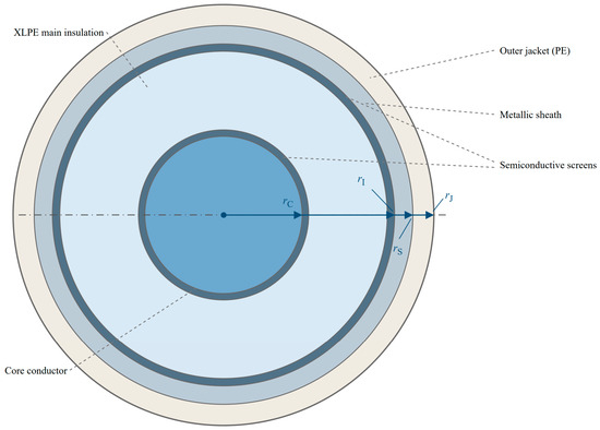
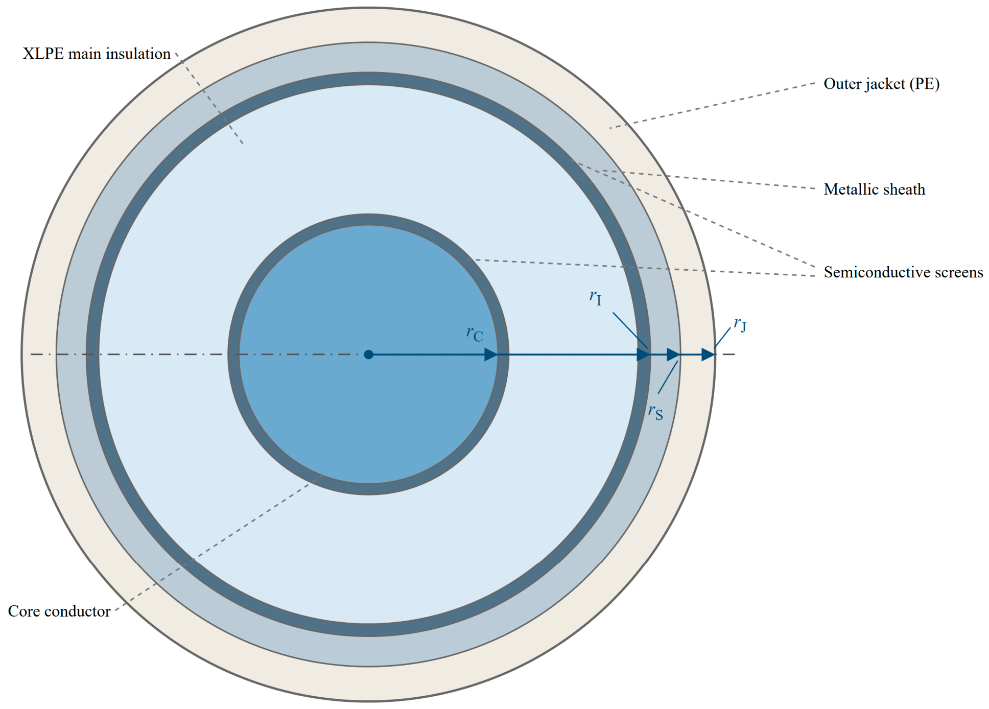
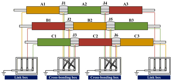
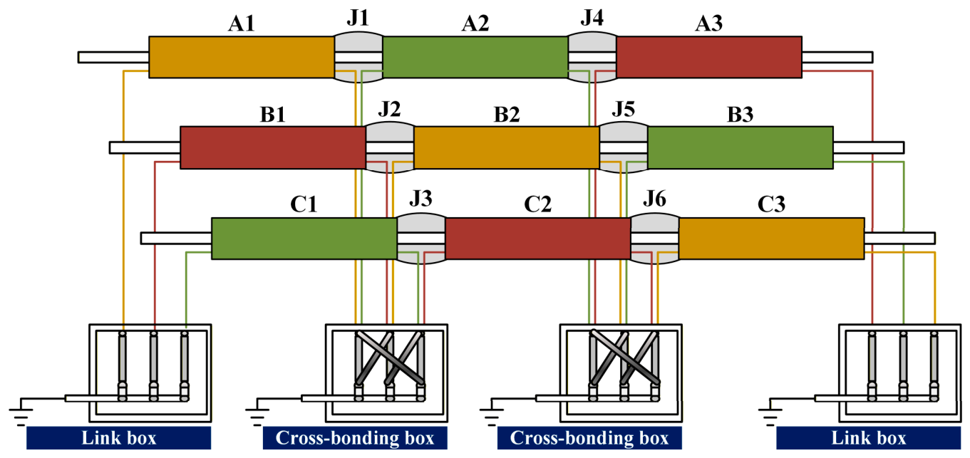
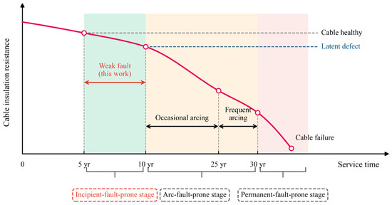
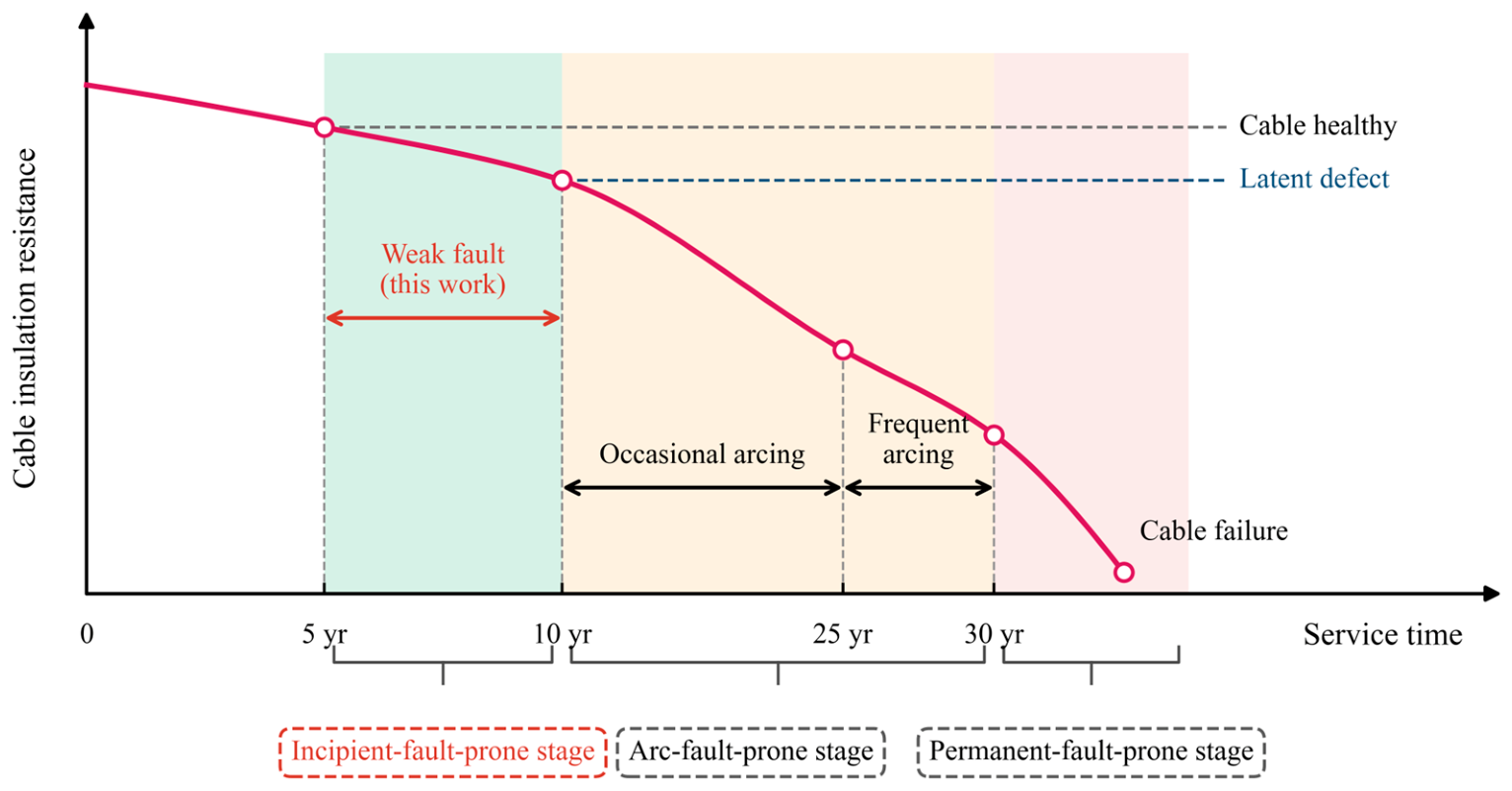
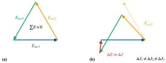
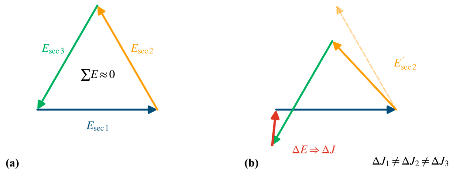
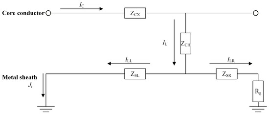
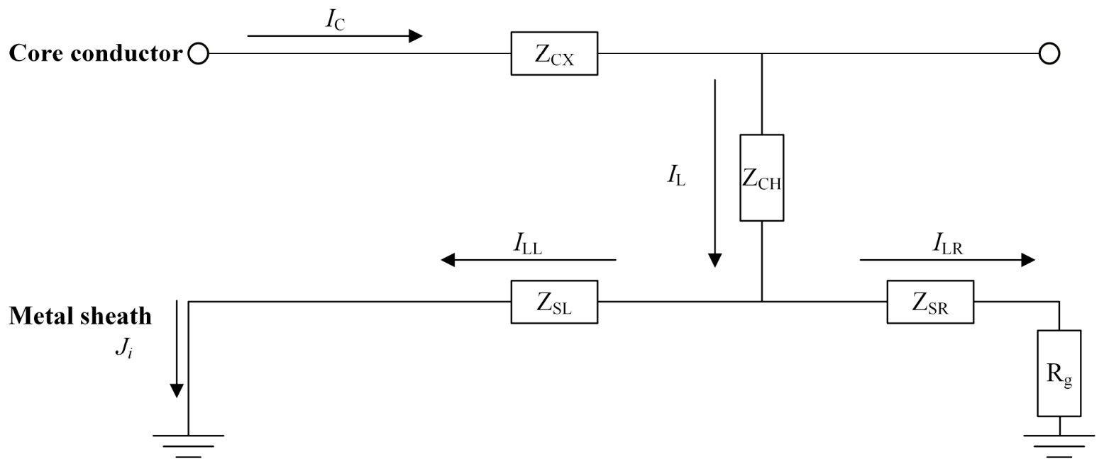
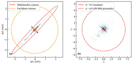
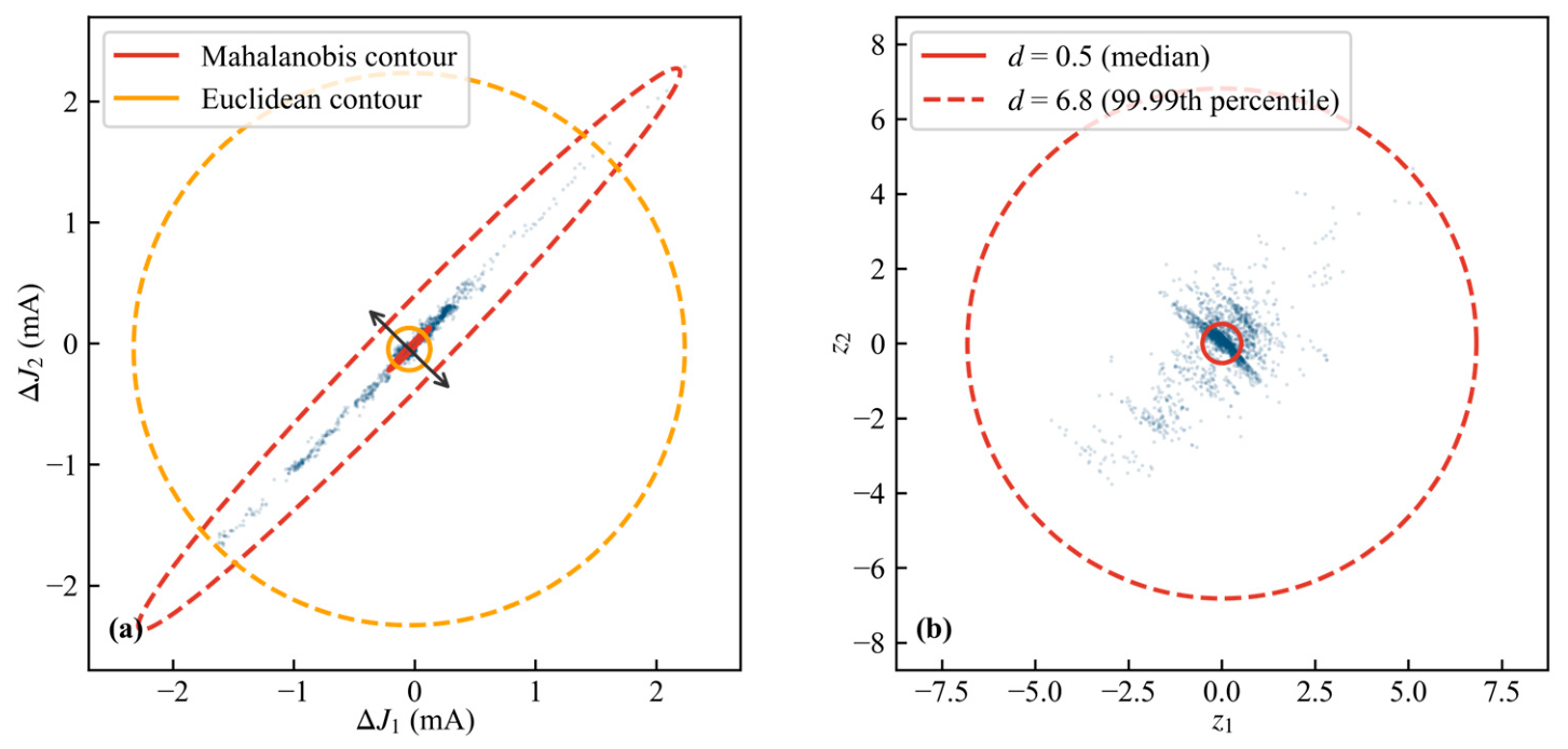
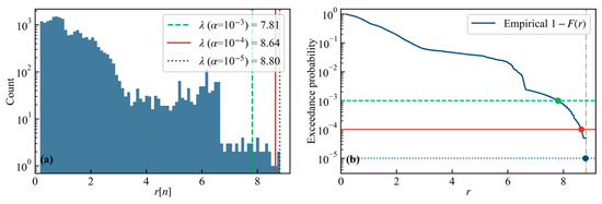
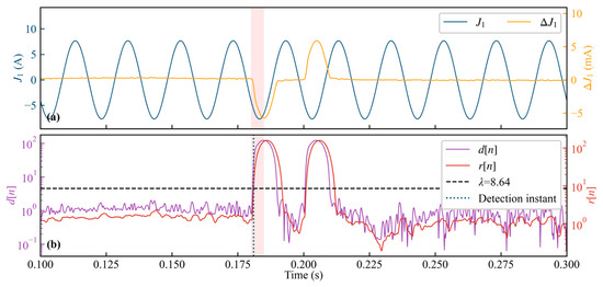
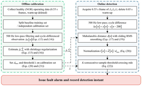
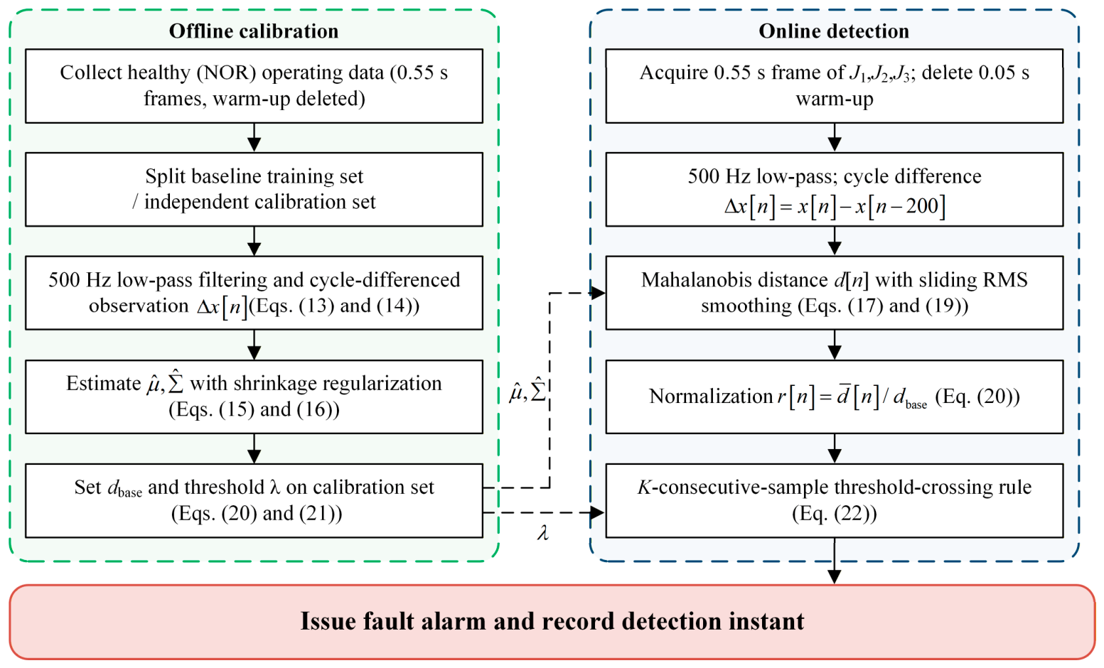
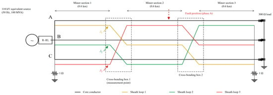
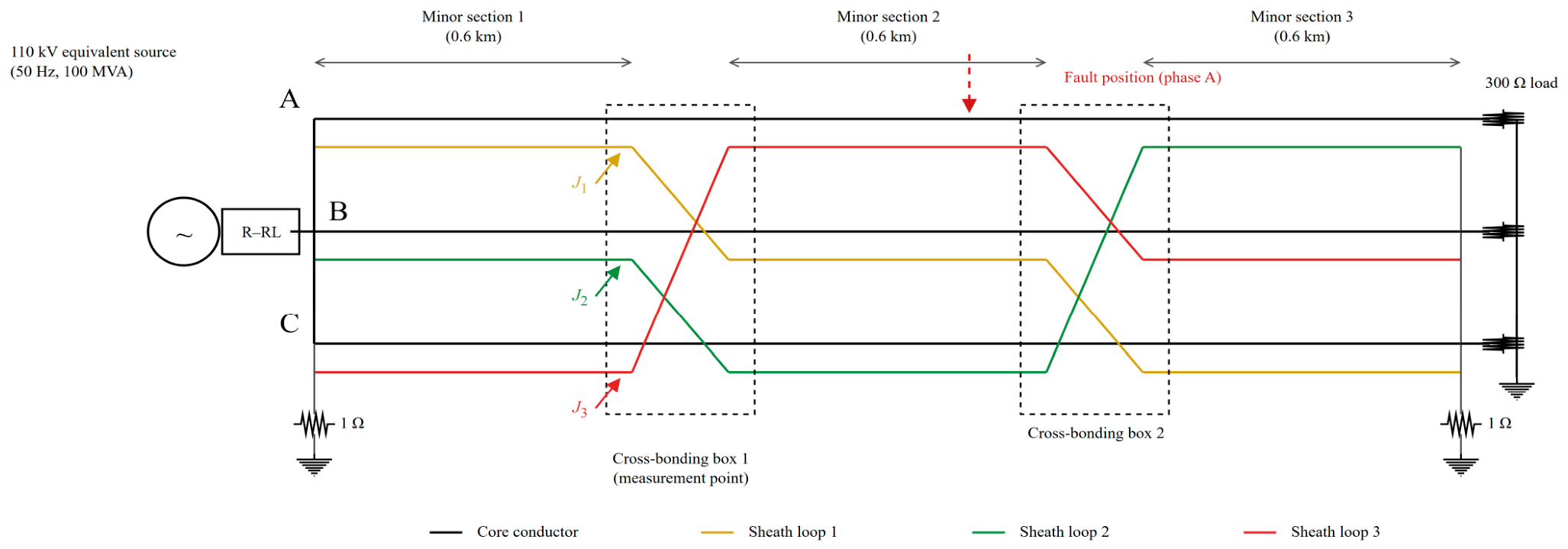
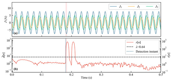
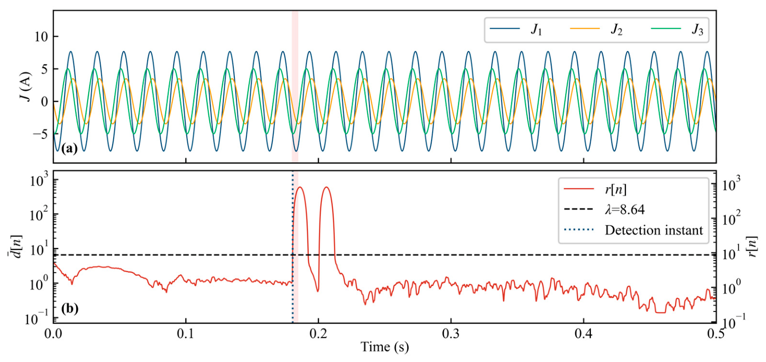
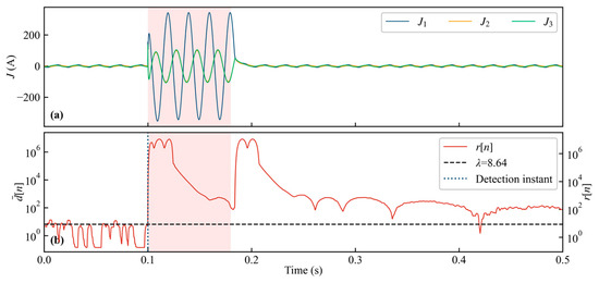
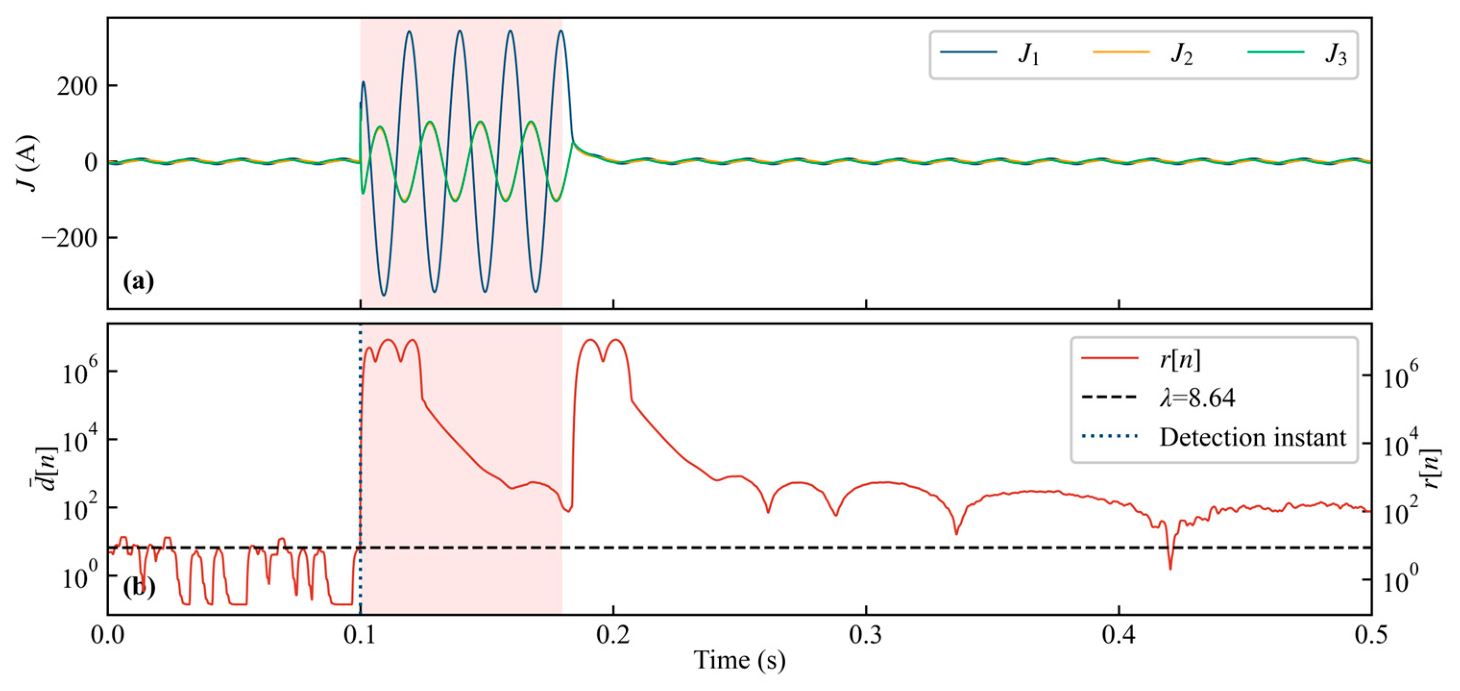
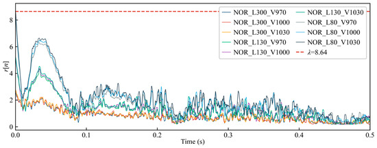
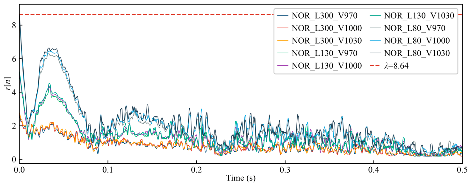
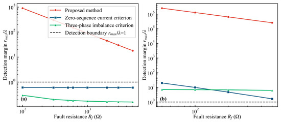
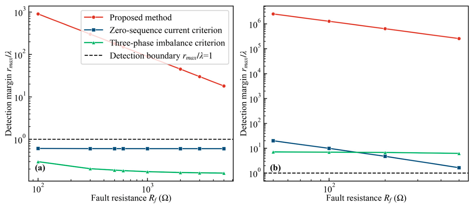
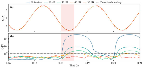
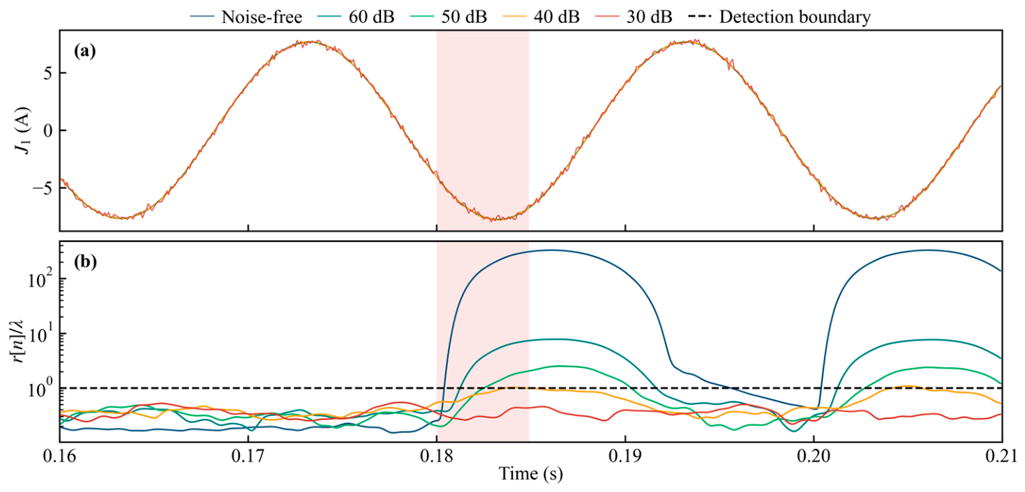

Disclaimer/Publisher’s Note: The statements, opinions and data contained in all publications are solely those of the individual author(s) and contributor(s) and not of MDPI and/or the editor(s). MDPI and/or the editor(s) disclaim responsibility for any injury to people or property resulting from any ideas, methods, instructions or products referred to in the content. |
© 2026 by the authors. Licensee MDPI, Basel, Switzerland. This article is an open access article distributed under the terms and conditions of the Creative Commons Attribution (CC BY) license.