


Abstract
With the large-scale integration of grid-forming wind turbines via LCC-HVDC transmission, the large-disturbance stability of such systems has become a critical concern due to complex interactions among multiple power electronic converters. This paper proposes a unified stability analysis framework based on the mixed potential function theory for a VSG-DFIG fed LCC-HVDC system under AC voltage sags at the point of common coupling. By incorporating the physical dynamics and constant-current control of the rectifier, and equivalently representing the PI controllers of the VSG-DFIG as RLC circuits, an equivalent circuit model of the entire system is established. The large-signal stability criterion is then derived, which explicitly reveals the influences of control parameters, circuit parameters, and the depth of AC voltage sags on the stability boundary. To enhance system stability, a virtual resistor strategy is introduced in the LCC-HVDC control loop. Finally, time-domain simulations in Simulink are carried out, and the results fully validate the theoretical analysis as well as the effectiveness of the proposed virtual resistor scheme.
1. Introduction
With the global energy transition accelerating wind power capacity expansion, remote renewable bases often rely on long-distance LCC-HVDC transmission to load centers due to inverse geographical distribution; LCC-HVDC is mature, high-capacity and low-loss, making it a primary solution. Meanwhile, declining synchronous generator penetration has promoted grid-forming control, which can autonomously establish voltage/frequency and support LCC-HVDC commutation [1,2]; VSG-controlled DFIGs emulate synchronous machine inertia/damping to provide frequency/voltage support under weak-grid conditions [3,4,5,6]. However, such grid-forming DFIG-based LCC-HVDC systems are nonlinear, multi-state, multi-converter, high-order systems with numerous control loops across wide time scales, giving rise to complex interactions among converters and with the AC grid [7,8,9]. Under large disturbances—e.g., AC voltage sags or DC line faults—these interactions may readily induce oscillations or even instability, making it urgent to accurately assess large-disturbance stability and develop effective enhancement measures.
With regard to the stability of grid-forming wind turbines integrated with LCC-HVDC systems, some explorations have been carried out by researchers. Reference [10] proposed a grid-forming control strategy for DFIG-based wind farms to enhance the stability of the LCC-HVDC sending-end system, and pointed out that grid-forming control can reduce the dependence of the sending-end system on synchronous generators. References [11,12] established an impedance network model of the AC grid at the sending end of an LCC-HVDC system incorporating grid-forming energy storage systems, and analysed the dynamic interactions among the wind farm, the weak AC grid and the LCC-HVDC link. For the oscillation issues in grid-forming direct-drive wind farms connected via LCC-HVDC, references [13,14] investigated subsynchronous oscillation characteristics and suppression strategies using the impedance method and time-domain simulation, respectively. However, the above studies mainly focus on small-signal stability or frequency-domain analysis of specific oscillation modes. There is still a lack of research on the transient stability of the system under large disturbances based on a unified modelling framework using the mixed potential function theory and corresponding analytical criteria.
For the large-disturbance stability analysis of power-electronic-based power systems, existing methods mainly fall into two categories: time-domain simulation and direct methods. Time-domain simulation methods (e.g., electromagnetic transient simulation) offer high accuracy and strong applicability, but they are computationally intensive and cannot easily reveal the underlying instability mechanisms [15]. Among direct methods, Lyapunov’s direct method can provide analytical stability criteria, but it lacks a unified modelling framework and it is often difficult to construct suitable Lyapunov functions for high-order nonlinear systems [16,17]. In contrast, the Brayton–Moser mixed potential function theory provides a unified approach for transient stability analysis of nonlinear circuits [18,19]. By constructing a unified potential function for inductors, capacitors and non-energy-storing elements in the circuit, this method can derive analytical large-disturbance stability criteria and has been widely applied to the large-disturbance stability analysis of power-electronic systems, such as DC microgrids [20,21], modular multilevel converters (MMC) [22], and all-DC wind power generation systems [23,24]. Although the mixed potential function theory has been preliminarily applied in DC microgrids, MMC and all-DC wind power systems, none of those systems simultaneously involve the VSG control characteristics of grid-forming DFIG and the converter dynamics and constant-current control of LCC-HVDC. The grid-forming DFIG-based system with LCC-HVDC transmission exhibits dual features, namely “autonomous voltage support characteristics of grid-forming sources” and “negative damping and commutation dynamics of line-commutated converters”. Its large-disturbance stability is affected not only by VSG inertia/damping parameters and PI parameters of the voltage and current double-closed-loop control, but also by the LCC constant-current control parameters and physical parameters such as commutation reactance. The coupling mechanism between these factors has not yet been revealed by existing mixed potential function models. Moreover, current studies mostly focus on stability analysis of systems dominated by a single type of converter; for cascaded converter systems consisting of grid-forming sources and line-commutated converters, there is a lack of unified modelling methods that can simultaneously account for both control dynamics and main-circuit physical dynamics.
Based on the above analysis, this paper proposes a large-disturbance stability analysis method for grid-forming DFIG-based systems with LCC-HVDC transmission using the mixed potential function theory. First, the physical dynamics and the constant-current control dynamics of the LCC-HVDC sending-end rectifier station are incorporated into the modelling to establish an improved load equivalent circuit model. Second, by exploiting the mathematical duality between controllers and circuits, the VSG control and the voltage-current double-closed-loop control of the VSG-DFIG are virtually equivalent to RLC circuits, thus building an equivalent circuit model that includes both control system and main-circuit parameters. Then, based on the mixed potential function theory, a large-signal stability criterion for the system is derived, revealing the influence laws of control parameters and main-circuit parameters on the stability boundary. Finally, to overcome the inherent limitations of traditional parameter optimisation strategies, a stability enhancement strategy with an additional virtual resistor is proposed, and SIMULINK simulations are carried out to verify the correctness of the theoretical analysis and the effectiveness of the proposed strategy.
2. Structure of the Sending-End System
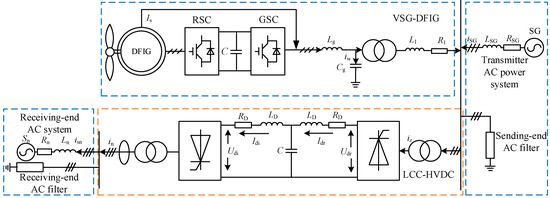
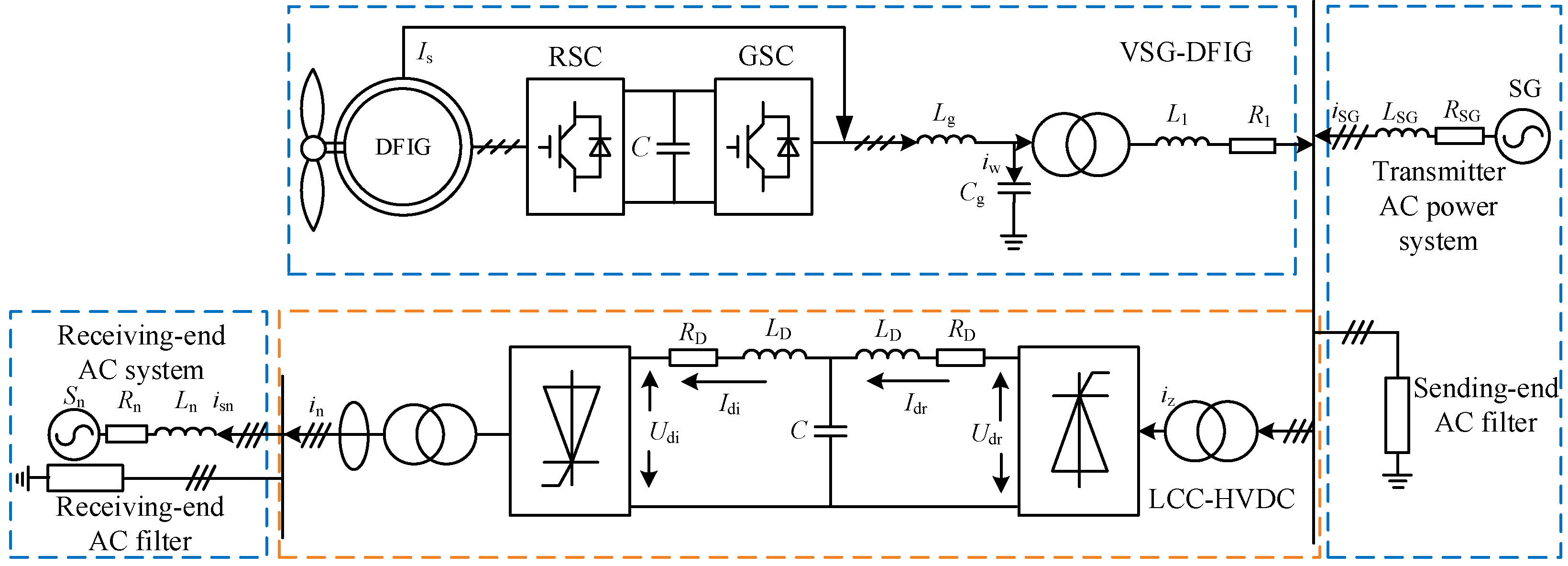
The system under study in this paper typically consists of components such as VSG-DFIG, thermal power units, AC filters, and LCC-HVDC, and the system topology is shown in Figure 1.
Figure 1.
Sending-end integration system topology.
As shown in Figure 1, traditional thermal power plants and VSG-DFIG are connected in parallel at the AC bus and are connected to the sending end of LCC-HVDC; the receiving end of LCC-HVDC sends power to the AC power grid of the load. The outer loop of VSG-DFIG adopts q-axis-oriented VSG control, and the inner loop is voltage-current dual closed-loop control. The rectification station at the sending end of LCC-HVDC adopts constant current control, and the inverter station at the receiving end adopts constant voltage control.
This system has many power electronic devices and a complex structure. To address the challenges brought by “multiple state variables, multiple converters, and high order” to the stability analysis of the DC system for large signals, many studies have adopted simplified reduced-order models to analyze the system stability [18]. Therefore, based on the existing research results, this paper simplifies the sending system to an equivalent single-source-load two-terminal cascaded system [19,20,21,22].
3. Based on the Virtual Equivalent of the Controller, the Equivalent Circuit Model of the Output System Is Established
3.1. LCC-HVDC Virtual Equivalent Circuit Model
For a grid with loads, the common modelling approach is to simplify the load converter as an ideal controlled current source, whose current response dynamics can be described as , In this paper, considering the physical dynamics and control dynamics of the LCC-HVDC sending-end rectifier station, an improved mathematical model is derived. Taking into account the constant-current control and the physical characteristics of the sending-end rectifier station, its mathematical model is given as follows:
where αr is the output angle of the constant-current controller, Idcref is the DC current reference, Idr is the rectifier-side DC current, KTr is the transformer ratio of the rectifier station, xcR is the commutation reactance, Kpr, Kir are the proportional and integral gains of the constant-current controller, Ld, Rd are the inductance and resistance of the smoothing reactor, Ud is the DC voltage, and Upcc is the AC voltage at the point of common coupling. Solving the second differential equation in Equation (1) yields:
Among them:
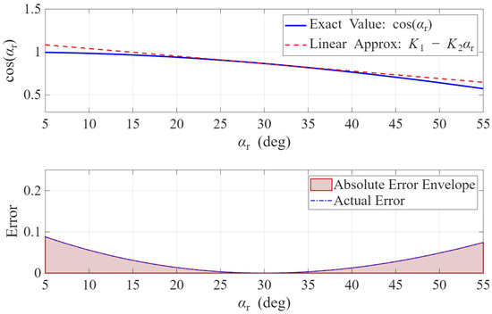
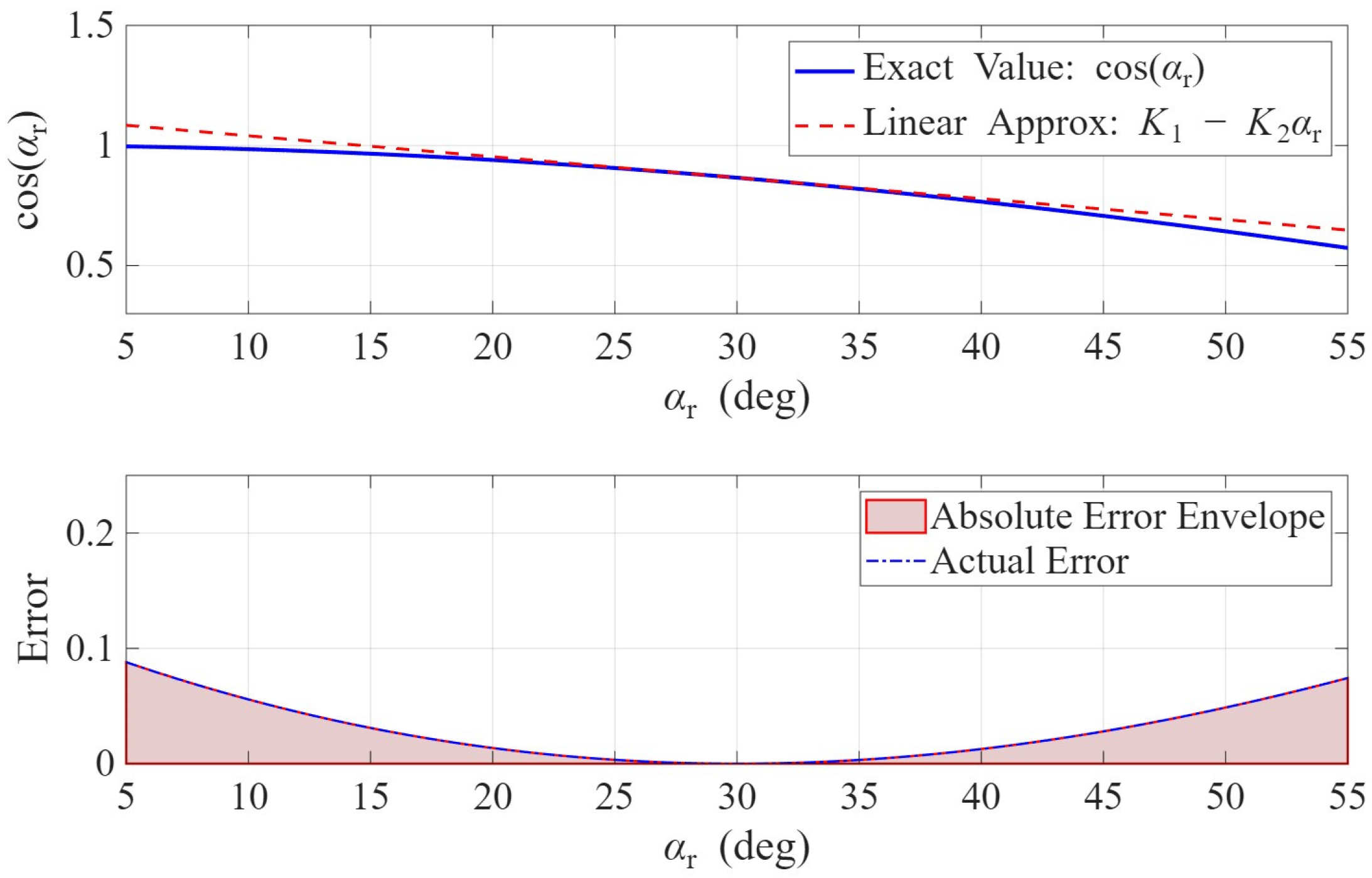
To obtain explicit expressions for the mixing potential function and the analytical expression of the stability boundary, this paper performs a first-order Taylor expansion of the trigonometric functions related to the trigger angle near the steady-state operating point. If the complete nonlinear form is retained, the subsequent differential equations and the stability boundary will contain transcendental functions, which is not conducive to analytical derivation. Considering the expansion of around , we have:
where K1 = , K2 = .To verify the feasibility of this linear expansion in the case of large disturbances, this paper plots the error curve of αr0 within the range of 5 degrees to 55 degrees using = 30 degrees as an example, as shown in Figure 2. The assessment indicates that the maximum error does not exceed 10% under extreme physical boundaries, thus this approximation has acceptable accuracy within the main research scope of this paper.
Figure 2.
Error curve graph.
Substituting Equations (2) and (4) back into Equation (1) enables the solution to be obtained, thereby deriving the mathematical model of the improved model that takes into account the physical dynamics and control dynamics of the converter:
Among them:
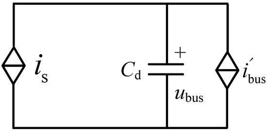
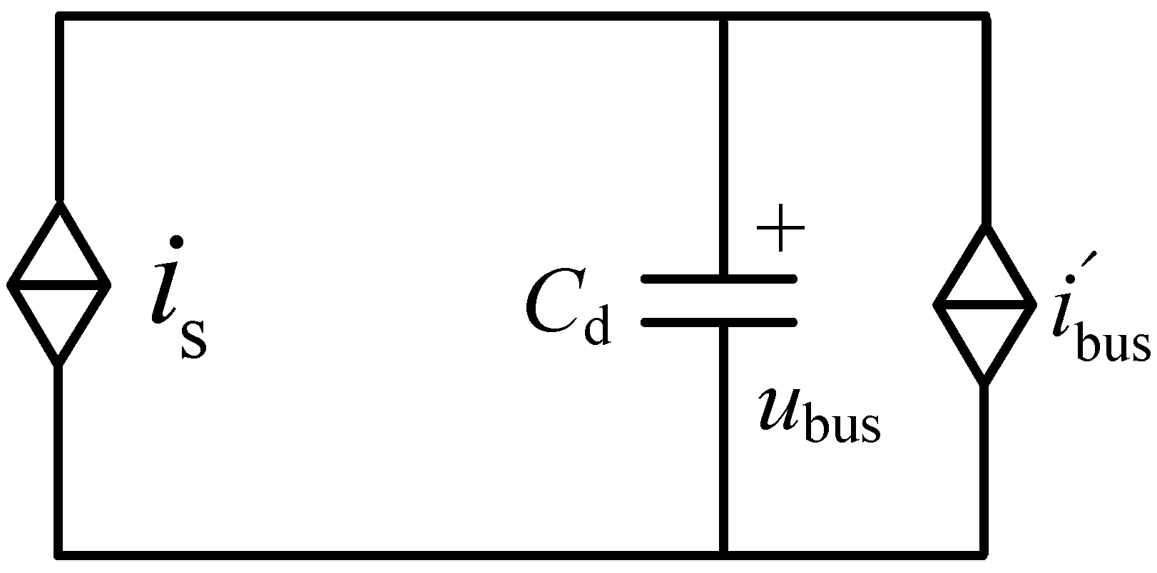
LCC-HVDC, as a load for absorbing power, its improved equivalent circuit model is shown in Figure 3.
Figure 3.
Improved equivalent circuit.
3.2. VSG-DFIG Virtual Equivalent Circuit Model
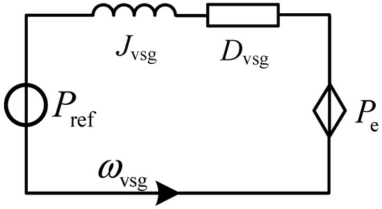
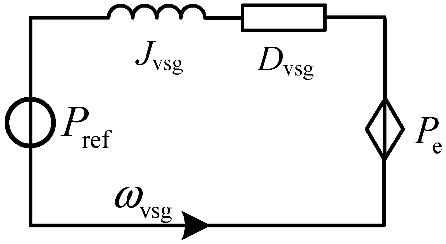
The traditional mixed potential analysis is unable to take into account features similar to those of synchronous machine rotation characteristics. The key control component of grid-connected wind turbines is the VSG control that simulates the rotation characteristics of an electric motor. This paper uses a method analogous to the actual circuit to model the VSG control. The outer loop power loop control equation of VSG is shown to be similar to the physical equation of the RL circuit as Equation (7):
where Ls, is, uout, us, Rs denote the inductance, current, input/output voltages and equivalent resistance of the equivalent circuit, respectively; Jvsg is the VSG inertia coefficient, Dvsg is the VSG damping coefficient, Pref is the active power reference of the VSG-DFIG, Pe is the active power of the VSG-DFIG, and ωvsg is the virtual angular frequency. Observing Equation (7), it can be found that the outer-loop power control equation of the VSG is exactly consistent in mathematical form with the physical equation of an RL circuit. Therefore, the inertia coefficient Jvsg can be analogised to the circuit inductance Ls, the damping coefficient Dvsg to the circuit resistance Rs, the virtual angular frequency ωvsg to the current is flowing in the circuit, the rated power Pref to the voltage source uout, and the output active power Pe to the output voltage. The equivalent circuit is shown in Figure 4.
Figure 4.
VSG control equivalent circuit.
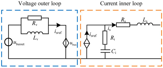
For the inner-loop voltage and current double-closed-loop control of the VSG, the mathematical model of the typical proportional-integral (PI) controller is essentially equivalent in physical nature to an RLC circuit. Therefore, in this paper the source-converter control system is virtually equivalent to an RLC circuit. The voltage error signal is obtained by taking the difference between the feedback voltage and the reference voltage , After passing through the PI controller, it outputs the current inner-loop reference current . Its mathematical model is given as:
where kvp, kvi are the proportional and integral coefficients of the voltage loop. Note that for a parallel RLC circuit, the voltage across each element is , and the sum of the currents in the parallel branches can be expressed as:
By comparing Equations (8) and (9), it can be seen that the voltage outer-loop PI controller and the parallel RL branch have the same mathematical form. Therefore, for the voltage outer-loop controller of the source converter, the virtual equivalent of the parallel RL branch can be used, and the duality relationship between the two is:
Similarly, the current inner-loop control compares the feedback current with the reference current to obtain the current error signal , After being regulated by the PI controller, outputs the control voltage signal . There exists a factor k between and the converter bridge-arm output voltage . Converting this relationship into the parameters of the control loop yields:
where kip, kii are the proportional and integral coefficients of the current loop. For the series RC circuit shown on the right side of Figure 5, the current flowing through each element is , so the voltage across the series branch can be expressed as:
Figure 5.
Dual-closed-loop control equivalent circuit.
By comparing Equations (11) and (12), it can be seen that the current inner-loop PI controller and the series RC branch have the same mathematical form. Therefore, for the current inner-loop controller of the source converter, the virtual equivalent of the series RC branch can be used, and the duality relationship between the two is:
At this point, a network-type equivalent circuit model of the wind turbine, including the control system and main circuit parameters, has been established. From Equations (8)–(13), the voltage-current dual closed-loop control of the inner loop of the VSG and the equivalent circuit model of the main circuit parameters can be obtained, as shown in Figure 5.
For the RL parallel circuit equivalent to the voltage loop shown in Figure 5, we have:
In the formula, iv represents the current in the inductor branch, and iv − iref represents the current flowing through the resistor branch.
4. Analysis of the Stability of the Overall System Signal
4.1. The Model of the System’s Mixed Potential Function for Transmission
4.1.1. The Theory of Mixed Potential Function
Compared with the direct Lyapunov method without a unified modeling approach, the theory of mixed potential functions provides a unified research method for the transient stability analysis of nonlinear circuits and can also provide stability criteria for nonlinear circuits under large disturbances. The mixed potential function is a special form of the Lyapunov function. Its application method is as follows: Based on the characteristics and structure of the nonlinear circuit, construct the mixed potential function of the system to be studied; then, according to the characteristics of the mixed potential function, reconfigure it to meet the required form of the corresponding stability discrimination theorem, and apply the corresponding theorem to obtain the stability criterion. The mixed potential function P is related to the circuit structure and can be constructed based on the inductors, capacitors, and non-storage elements in the nonlinear circuit. Its unified representation is:
where is the current potential function of the non-energy-storing elements in the nonlinear circuit; is the voltage potential function of the non-energy-storing elements in the circuit; is the product of voltage and current of capacitors and other non-energy-storing elements.
The mixed potential function theory has three stability theorems. In this paper, the third stability theory will be adopted to analyze the large disturbance stability of the system. For the convenience of subsequent application, it is restated as follows:
Define , , Let be the minimum eigenvalue of the matrix , and be the minimum eigenvalue of the matrix , where L is the diagonal matrix consisting of all inductances in the circuit, and C is the diagonal matrix consisting of all capacitances in the circuit. That is, if the circuit contains inductances , then L = diag().
If in the circuit, all the i and v satisfy:
Regardless of how the voltage and current of the circuit change, the system will eventually tend towards a stable equilibrium operating point, meaning that the system can ensure stability even under significant disturbances.
4.1.2. Output the System’s Mixed Potential Function
Taking into account Equation (14), the current potential function for all non-storage components in the system is:
The voltage potential function is the sum of the product of the voltages and currents of all capacitors, which is:
Combining Equations (17) and (18) and simplifying them, the mixed potential function P(i,u) can be obtained as shown in Equation (18).
From , we can conclude that:
Therefore, is:
The smallest eigenvalue of this matrix is:
When the system reaches a steady state, g(t) = G0 , since we will subsequently take partial derivatives, the value of G0 has no impact on the subsequent analysis. Combining with Equation (5), we have:
From , we can conclude that:
Therefore, the minimum eigenvalue of the matrix is:
By applying the third stability theory of the mixed potential theory, the large-signal stability criterion for the VSG-DFIG system transmitted via LCC-HVDC can be obtained as follows:
Equation (26) provides a complete set of system variables including system control parameters, main circuit parameters, and the improved load model, which serves as the criterion for the large-signal stability of the sending system. The units of each term in Equation (26) are all s−1. Based on this criterion, the influence of system parameters on the system stability boundary can be intuitively displayed. It should be noted that when Kpr or Upcc takes on small values, the denominator of Equation (26) may approach zero or even change sign. It is important to point out that this situation corresponds to the system already operating under severe large disturbances, at which point the system’s large-signal stability can no longer be guaranteed. Therefore, Equation (26) is used for stability assessment only within the domain where its denominator is nonzero and the system satisfies normal operating conditions; when Kpr or Upcc is too small, causing the denominator to approach zero or change sign, the operating condition should be directly considered to have exceeded the stable operating range, and Equation (26) should no longer be used for further stability margin assessment.
4.2. Stability Criterion Analysis
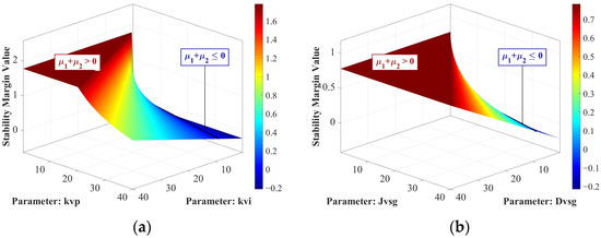
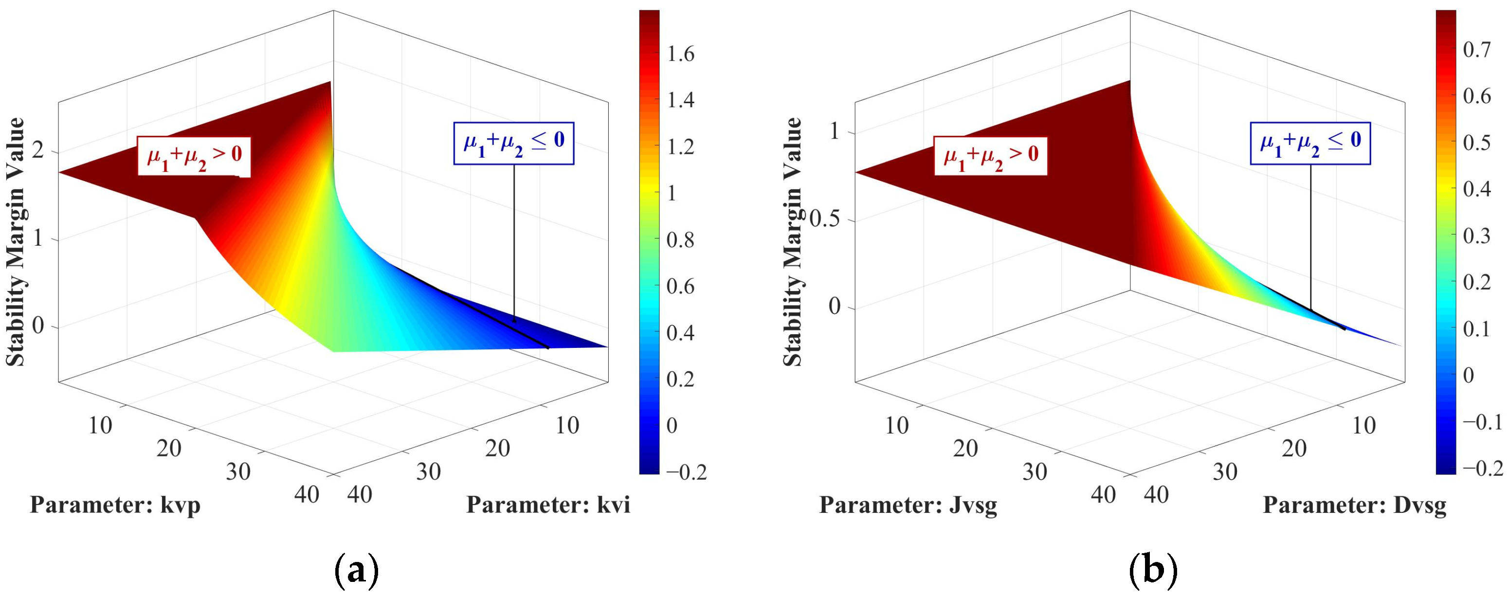
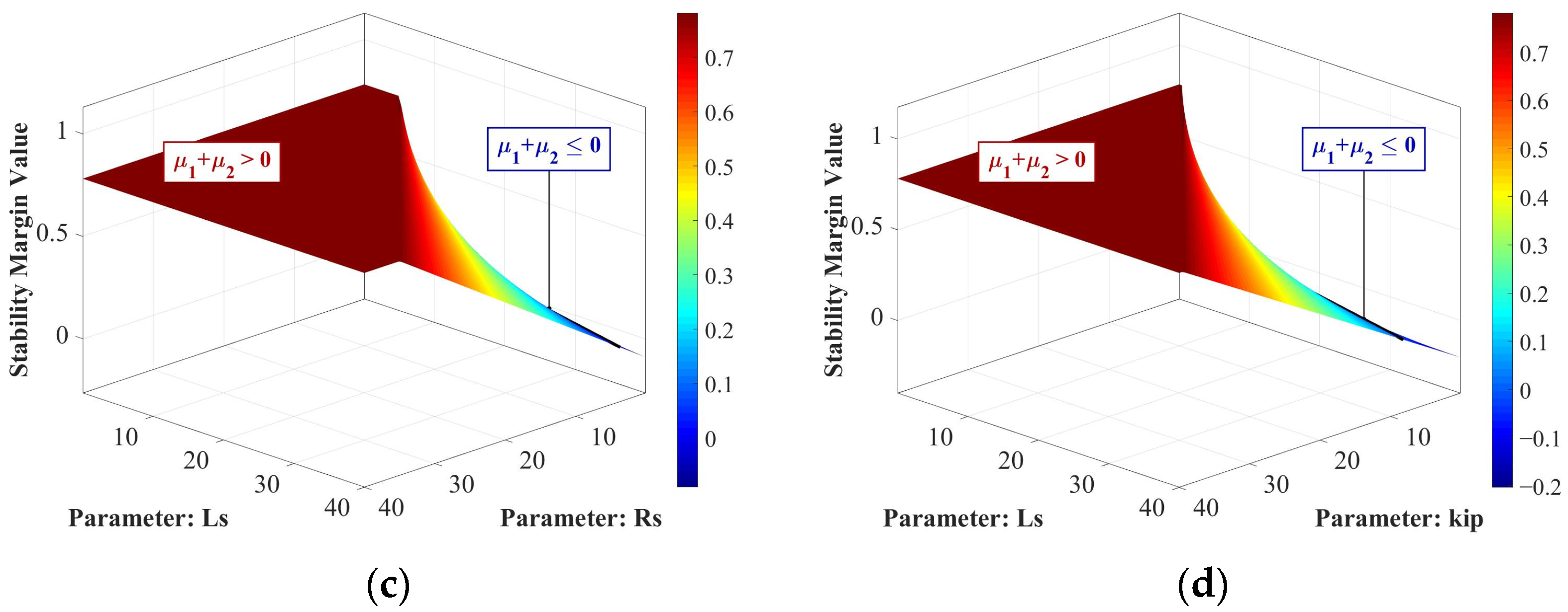
Based on Equation (26), the three-dimensional surface plots of versus four sets of parameters—namely kvi versus kvp, Jvsg versus Dvsg, LS versus RS, LS versus kip—are obtained as shown in Figure 6, where the region with > 0 indicates the stable domain of the system parameters. The parameter configurations are listed in Table 1.
Figure 6.
Three-dimensional stability analysis diagram. (a) kvp and kvi; (b) Jvsg and Dvsg; (c) Ls and Rs; (d) Ls and kip.
Table 1.
System Parameter Configuration Table 1.
As shown in Figure 6, within this parameter range, when the integral coefficient kvi of the voltage loop, the control inertia coefficient Jvsg of VSG, and the equivalent inductance LS are reduced, the will increase, which means that the large-signal stability of the system will be enhanced. When the proportional coefficient kvp of the voltage loop, the control damping coefficient Dvsg of VSG, and the proportional coefficient kip of the current loop are reduced, will decrease, and the large-signal stability of the system will be weakened. From the perspective of equivalent control parameters, the damping coefficient and the proportional coefficient can be regarded as line resistances. The difference is that the damping coefficient has a monotonically increasing relationship with the equivalent line resistance value, while the proportional coefficient has a monotonically decreasing relationship with the equivalent line resistance value. Increasing the damping coefficient and decreasing the proportional coefficient will increase the equivalent line resistance value, and the increase in line resistance within a certain parameter range will increase the system damping and can weaken the adverse impact of negative damping introduced by LCC-HVDC on the system stability, thereby enhancing the system stability.
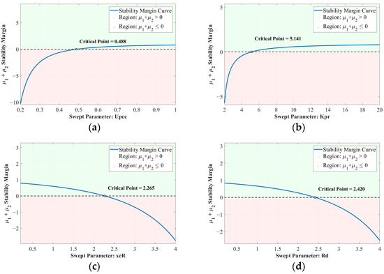
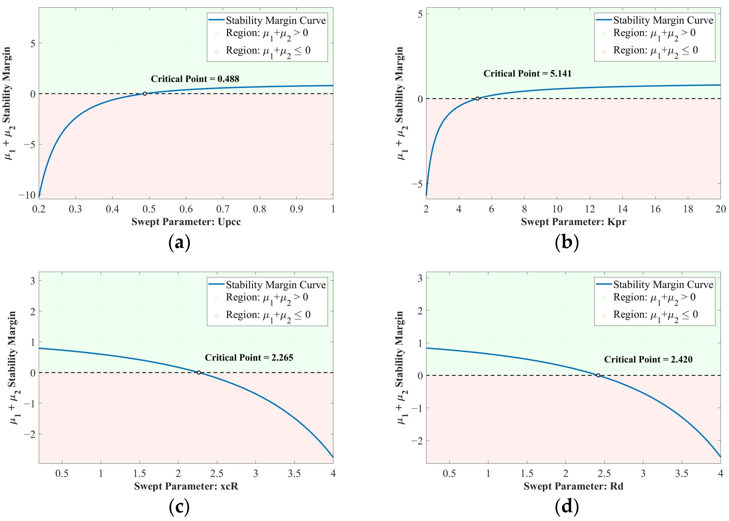
The trend of change for a single variable is shown in Figure 7. Within the parameter range, when the voltage sag depth is increased, the proportional coefficient Kpr of the fixed current control is decreased, the commutation reactance xcR is increased, and the smoothing resistance Rd is increased, the value of will decrease and the overall signal stability of the system will be weakened.
Figure 7.
Univariate stability analysis diagram. (a) Upcc; (b) Kpr; (c) xcR; (d) Rd.
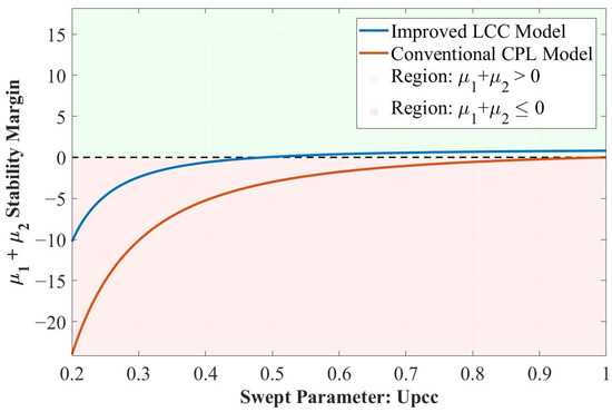
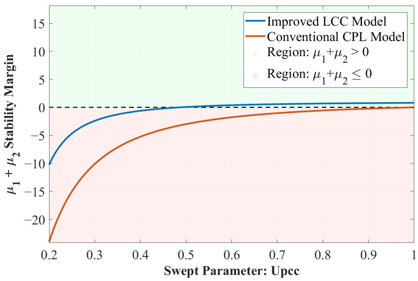
To verify the stability assessment capability of the proposed improved LCC equivalent model, this paper compares it with the traditional constant power load (CPL) model. The absorption current of the CPL model is:
In the formula, represents the constant power absorbed by LCC. Therefore, the value of the CPL model, denoted as , is:
Using the same PCC voltage variation range to calculate the large disturbance stability criteria for the two models respectively, the results are shown in Figure 8. The results indicate that the stability margin given by the traditional CPL model is overall lower than that of the proposed improved LCC model, that is, its predicted instability range is larger, demonstrating stronger conservatism. In contrast, the proposed model, considering the LCC constant current control and the physical characteristics of the converter, can avoid the excessive conservatism of the traditional CPL in stability assessment, thereby obtaining a stability boundary that is more in line with the actual operating characteristics.
Figure 8.
Comparison chart of different models.
Furthermore, the incremental characteristic of the traditional CPL model is mainly determined by the steady-state active power and the PCC voltage. Its stability criterion is difficult to reflect the independent effects of the LCC controller and the physical parameters of the converter. The proposed improved LCC model incorporates constant current control and the physical dynamics of the rectifier side into the equivalent model. Therefore, its stability criterion can further characterize the influence of control and physical parameters on the stability of the system under large disturbances, thereby providing a more comprehensive basis for stability boundary analysis and key parameter optimization. The starting point of proposing the improved LCC model in the original text is precisely to incorporate constant current control and the physical characteristics of the rectifier station into the equivalent model of the load.
4.3. Sending-End System Stability Enhancement Strategy
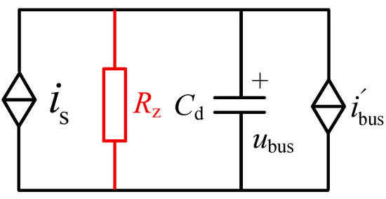
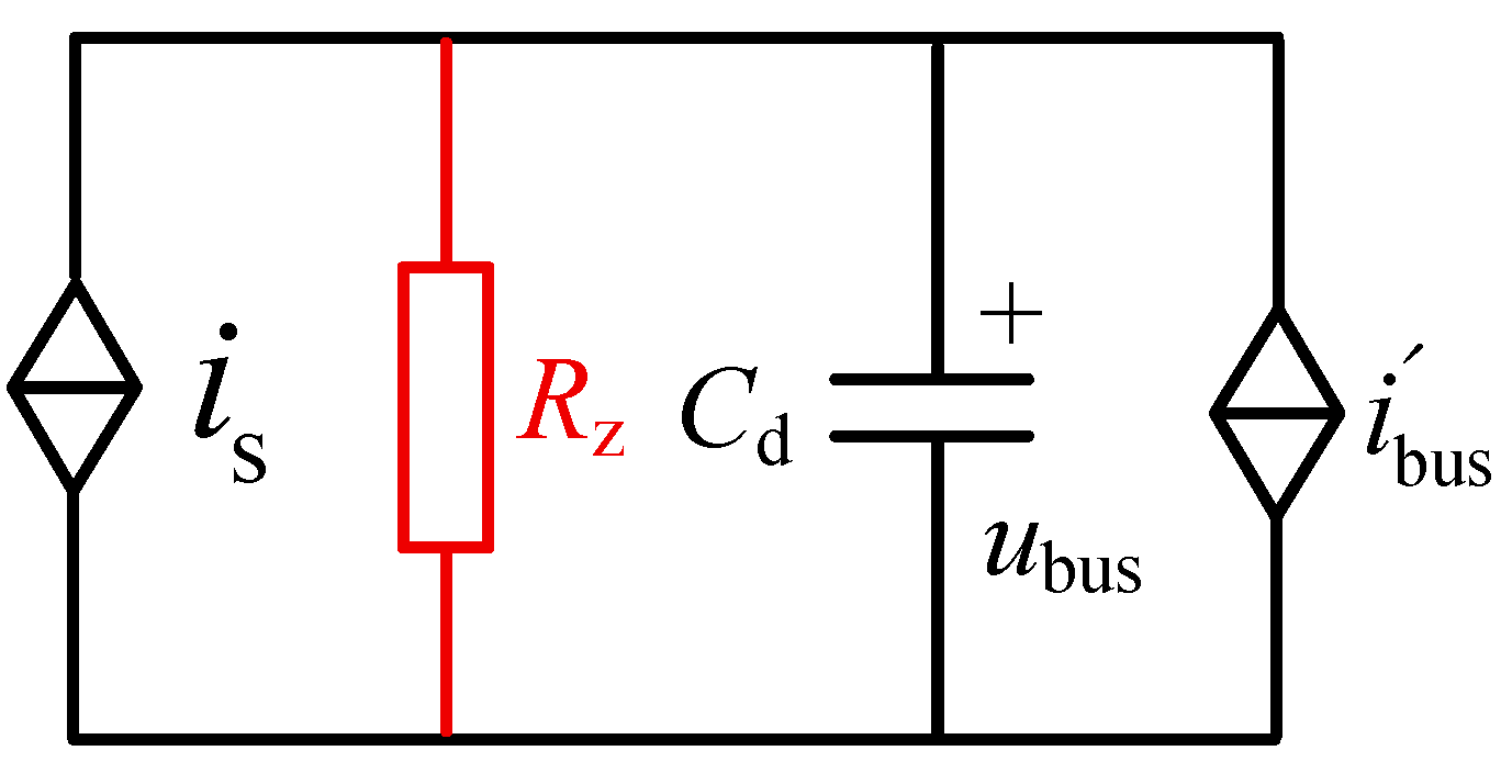
When the system is still in the design stage, the influence of the interaction of system parameters on the stability of the large signals can be analyzed to determine the range of key parameters, thereby enhancing the stability of the system. However, when the system is in operation, it is difficult to make changes to the system. At this time, the stability of the large signals of the system can be enhanced by optimizing the control parameters and using virtual resistors. A resistor Rz is paralleled on the LCC-HVDC side, as shown in Figure 9.
Figure 9.
Virtual Resistance Topology.
At this point, the criterion for judging the stability of the system’s large signals is:
If a virtual resistor is directly connected in parallel on the DC side, it will cause huge losses and is difficult to implement in practical engineering. Therefore, the scheme of connecting a resistor on the DC side needs to be realized in the control system. According to the law of power conservation, the power sent out by LCC-HVDC is equal to the power absorbed by the AC system. Thus, if the power required for constructing the virtual resistor is to be obtained, the power input to the AC grid on the AC side can be changed by adjusting the size of the DC current idr.
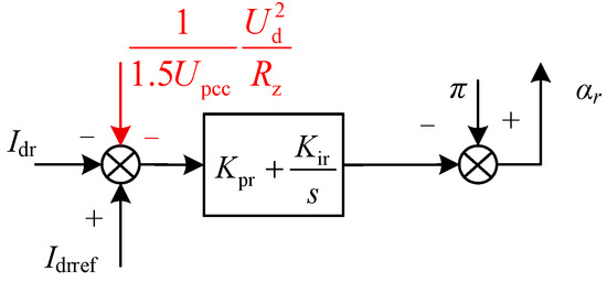
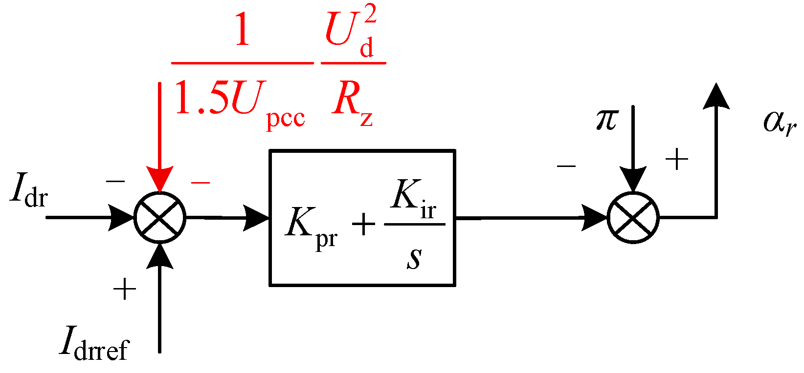
The control structure after adding the virtual resistance is shown in Figure 10. In the control structure of the LCC-HVDC rectification station, a current loop is added to achieve the design of the virtual resistance Rz. The expression of Δidr is:
Figure 10.
Control structure after adding virtual resistor.
To verify the transient equivalence of the virtual resistance control, the dynamic characteristics of the current controller and the control delay need to be taken into account. Firstly, the closed-loop transfer function of the current controller is defined as:
Define Gdel(s) as the equivalent delay of the control and sampling sections, and GLCC, I(s) as the incremental transfer function from the LCC control input to the DC current Idr. Then the closed-loop current tracking relationship is:
By linearizing Equation (30) around the steady-state operating point, we obtain:
Therefore, there is:
Further, the complete LCC incremental model is written as:
where represents the incremental transfer relationship of the current from I to the equivalent DC bus, and represents the additional incremental channels introduced by non-ideal factors such as commutation, voltage and power losses in LCC. The closed-loop port relationship of the actual virtual resistance can thus be obtained as:
In the formula, the closed-loop incremental port admittance formed by the actual virtual resistance control is:
To compare with the ideal physical parallel resistance, the dimensionless equivalent coefficient is defined as:
When the constant current controller has a sufficiently high closed-loop bandwidth within the main transient frequency band, there is , and when the increments of delay, converter losses, and reactive power coupling-induced deviations are relatively small, there is . In this situation, there is:
Thus, the additional term of the virtual resistance in the mixed potential function Hessian can be approximately written as , Therefore, in Equation (29), can be regarded as an approximation of the actual virtual resistance closed-loop increment port admittance within the normal linear operating region; when current saturation or significant dynamic delay occurs, this additional damping will be correspondingly weakened.
From Equation (30), the additional transmission power generated by the virtual resistance is . Therefore, there is:
The additional term for the stability criterion of the virtual resistance is . Therefore, its normalized sensitivity also is:
Therefore, reducing Rz can increase the stability margin, but it will increase the DC current demand and additional power consumption in proportion to 1/Rz. If the additional transmission power is limited to not exceeding of the original transmission power P0, then it should satisfy:
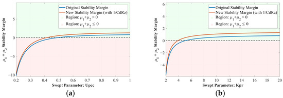
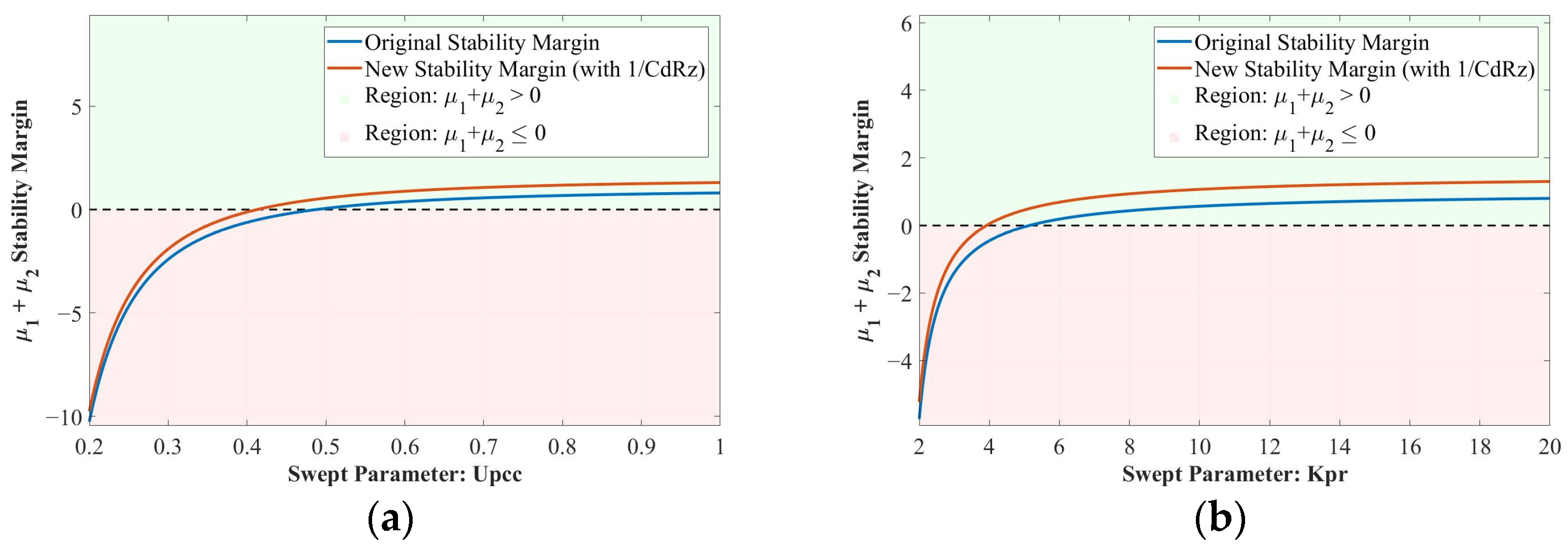
Based on the large disturbance stability criterion obtained from Equation (29), by substituting the parameters in Table 1, the change trend of the system’s large-signal stability criterion after adding a 5 Ω virtual resistor can be obtained, as shown in Figure 11.
Figure 11.
Comparison of Large Disturbance Stability Criteria. (a) Upcc; (b) Kpr.
By comparison, it can be seen that the addition of virtual resistors is beneficial for improving the stability margin of the system, thereby enhancing the stability of the system and increasing its operational limits.
5. Simulation Verification
This paper uses the MATLAB/SIMULINK 2017B platform to verify the correctness of the large-signal stability analysis presented in this paper and the effectiveness of the additional virtual resistance strategy.
5.1. Verification of Stability Analysis for the Overall System Signal
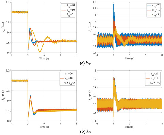
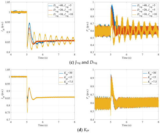
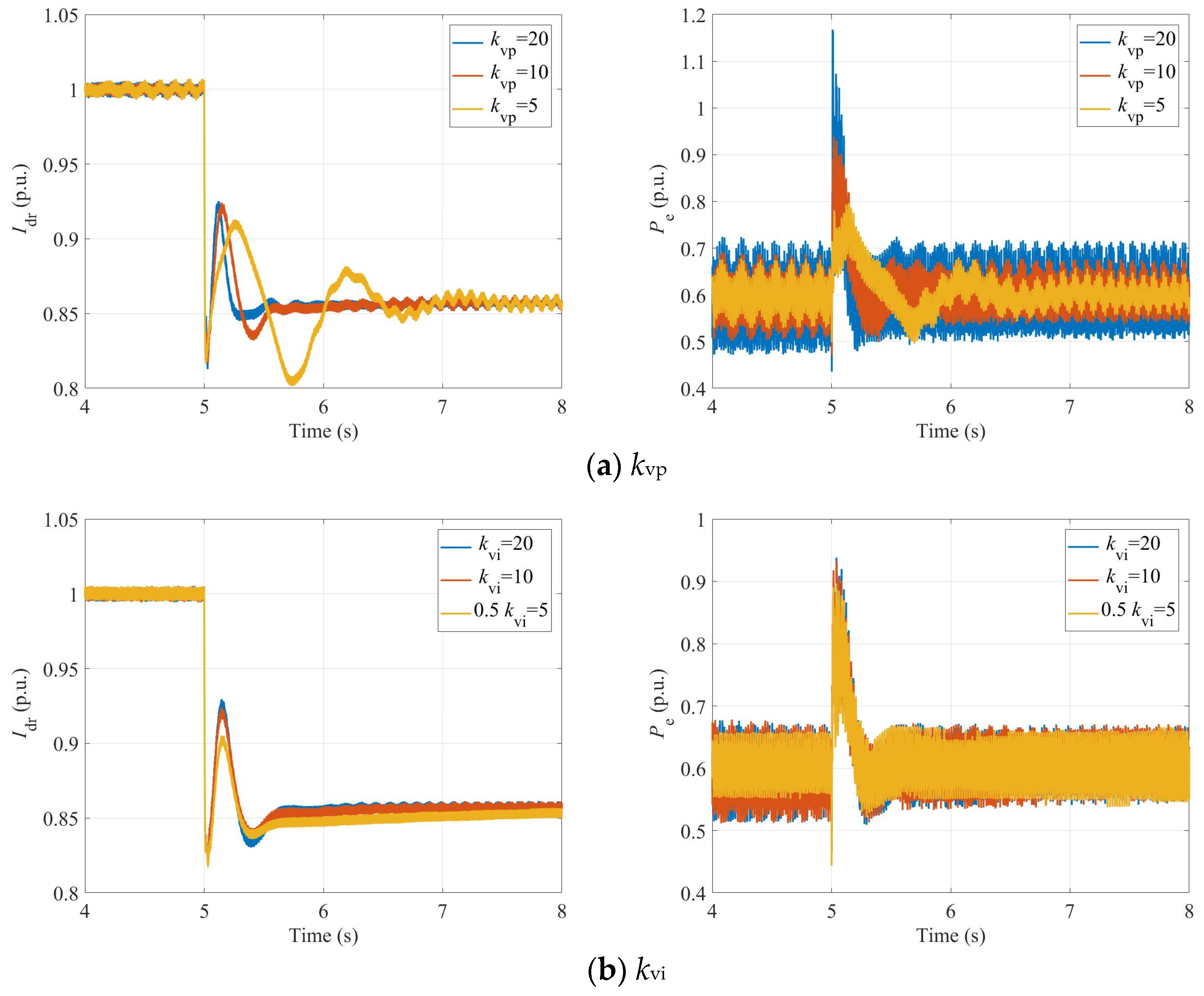
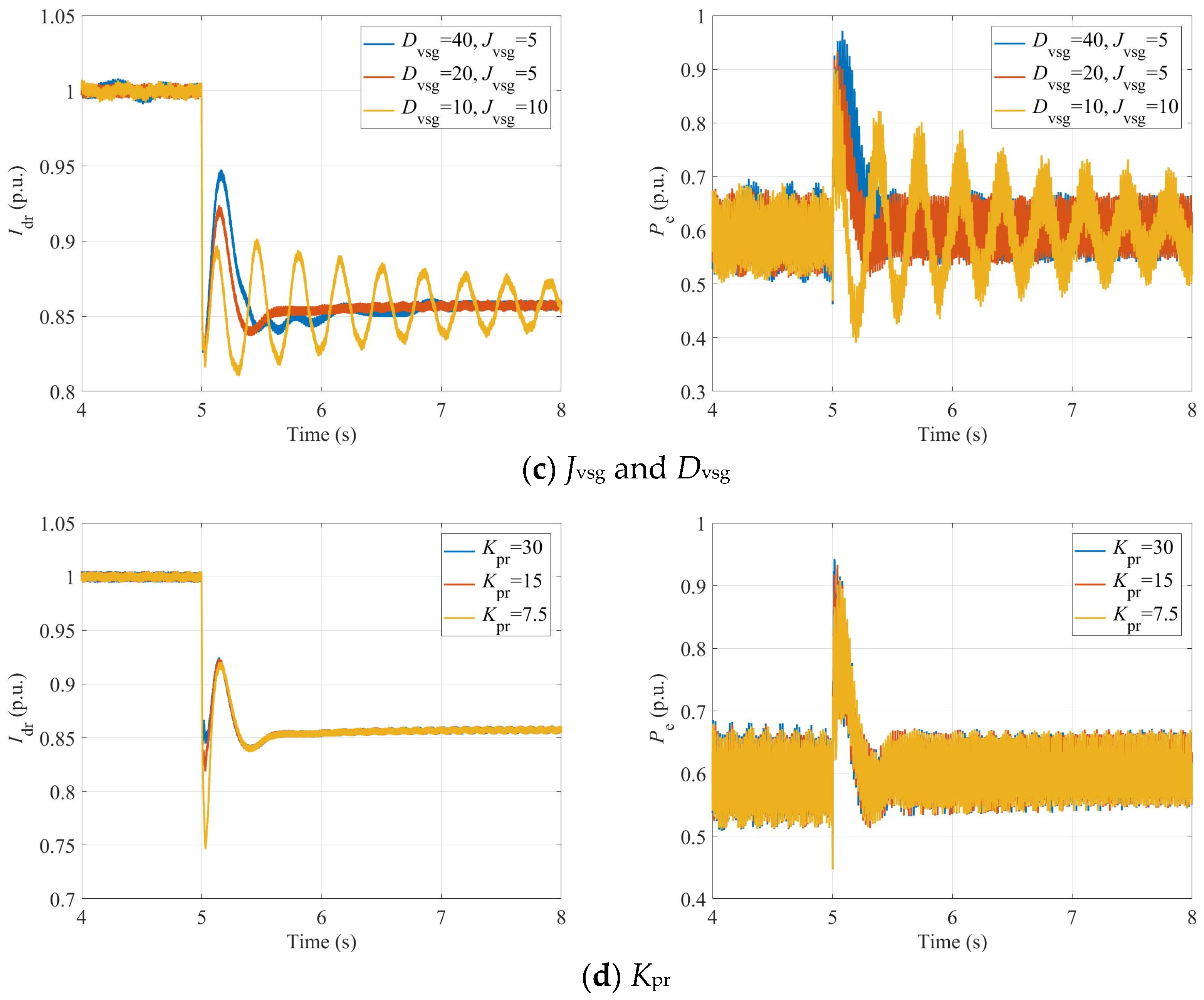
The system tie-point voltage was set to 0.6 pu at 5 s. Under different control parameters of the sending system, the active power Pe of the VSG-DFIG and the DC current Idr of the LCC-HVDC are shown in Figure 12.
Figure 12.
System Physical Waveforms as Control Parameters Vary.
As shown in Figure 12a–d, decreasing the voltage outer-loop proportional gain , increasing the voltage outer-loop integral gain , decreasing the VSG damping coefficient , increasing the VSG inertia , or decreasing the constant-current control proportional gain all significantly weaken the system’s large-disturbance stability. This trend is consistent with the theoretical analysis results presented in Section 4.2.
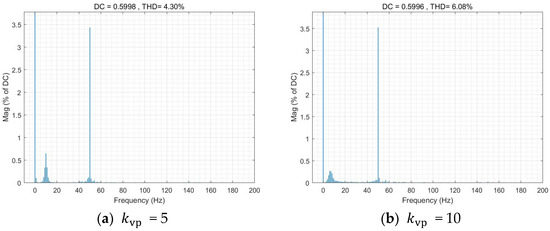
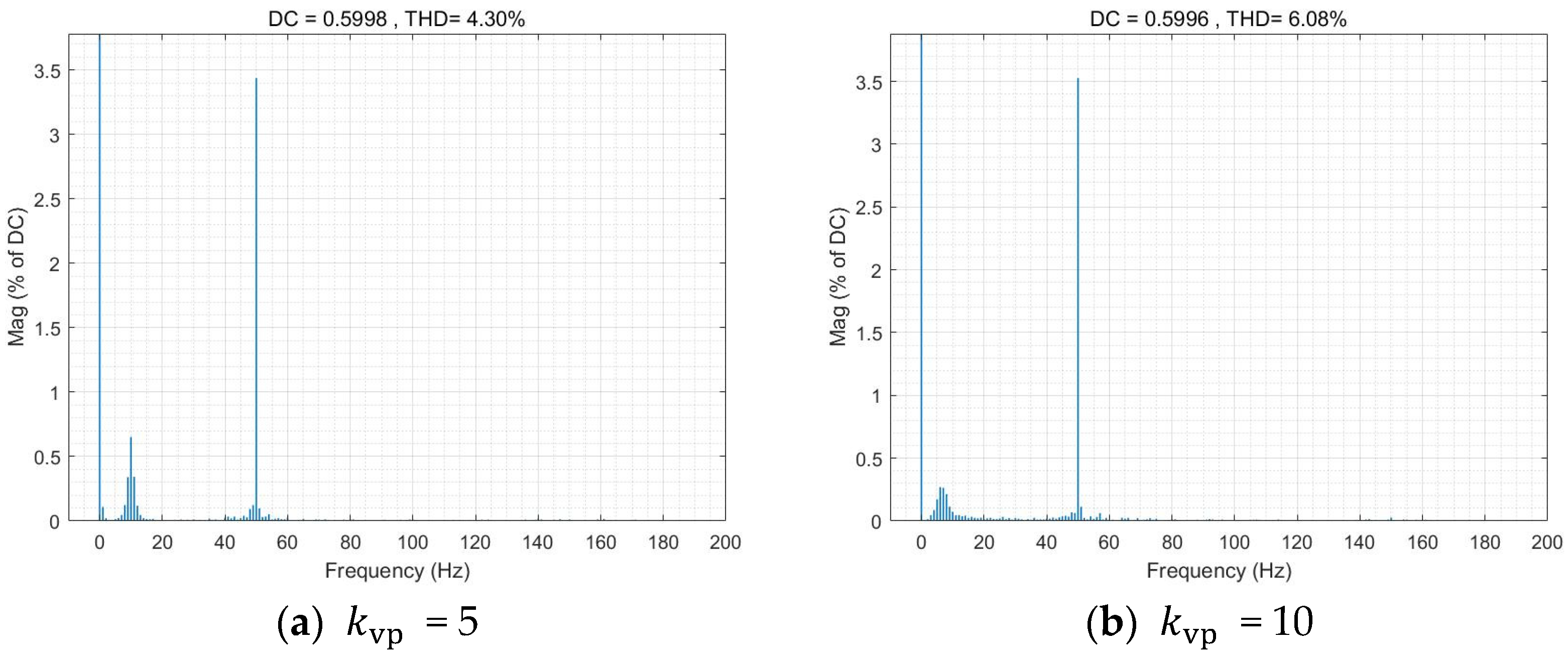
Further examination of Figure 12 reveals that although raising , lowering , or increasing can accelerate oscillation decay and improve the large-signal stability margin, these adjustments simultaneously exacerbate steady-state harmonic distortion considerably. Take as an example. When = 5 and = 10, the THD analysis of the system is shown in Figure 13.
Figure 13.
Analysis of THD under Different Control Parameters.
By combining Figure 12 and Figure 13, it can be shown that parameter optimization may improve the system’s stability under large disturbances, but may also compromise steady-state harmonic performance. This trade-off is precisely the inherent bottleneck faced by conventional parameter optimisation strategies, which highlights the necessity and rationality of the stability-enhancement methods proposed in this paper, such as the additional virtual impedance.
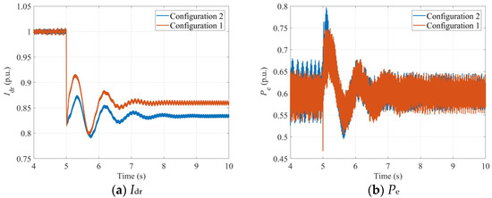
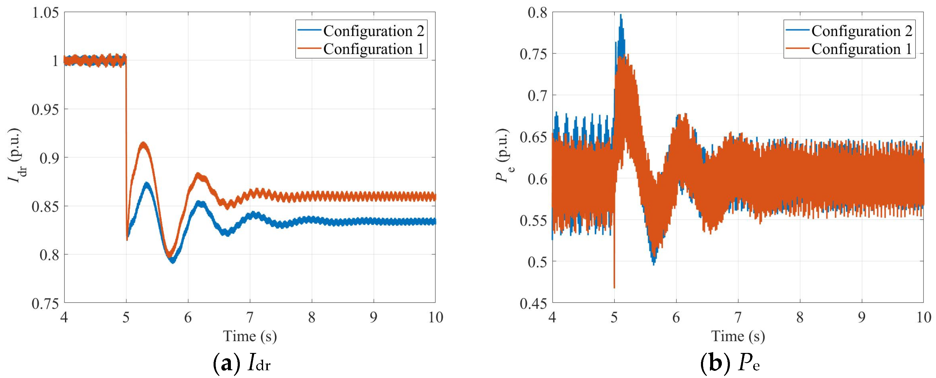
To investigate the influence of physical system parameters on large-signal stability, Configuration 1 uses Ls = 0.4, while Configuration 2 uses Ls = 0.6. Comparative experiments are conducted. The PCC voltage is again set to drop to 0.6 pu at s. The corresponding waveforms of the VSG-DFIG active power Pe and the LCC-HVDC DC current Idr are shown in Figure 14.
Figure 14.
System physical waveform as Physical Parameters Change.
Figure 14 further validates the theoretical analysis results in Section 4.2 regarding the influence of physical parameters on the stability of the system under large disturbances. Since in actual operation, the physical parameters of the system, such as line impedance and converter reactance, are usually difficult to adjust online, it is impossible to directly enhance the large-signal stability margin of the system by changing these parameters. Therefore, it is necessary to seek ways to enhance system stability from the control parameters or additional control strategy levels.
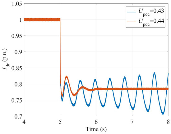
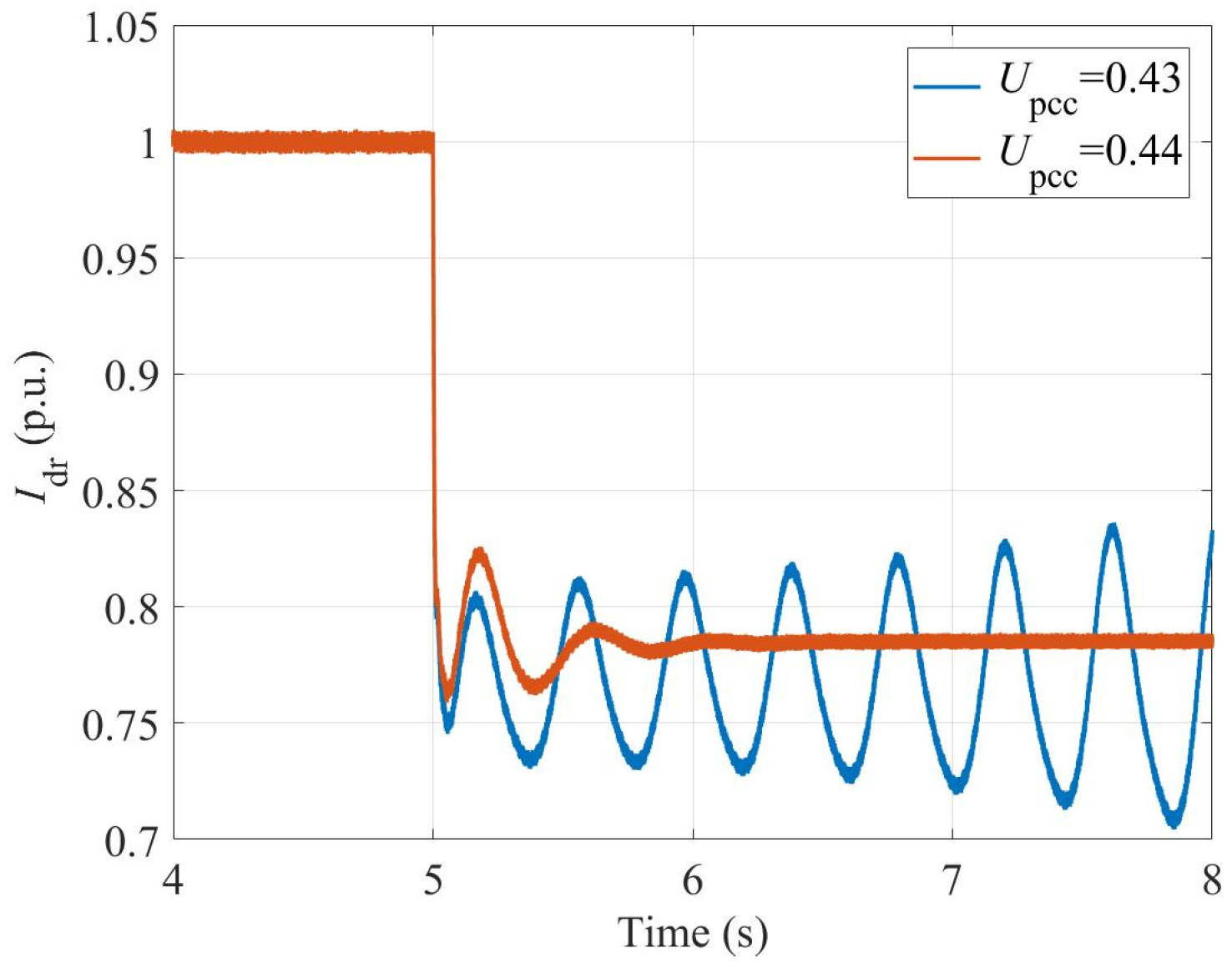
To quantitatively verify the accuracy of the large-signal stability criterion proposed in Section 4.2, the critical voltage drop depth under the parameter configuration of Table 1 was tested through time-domain simulation. The results are shown in Figure 15.
Figure 15.
Measurement of instability boundary.
As shown in Figure 15, when the voltage at the system’s common coupling point drops to approximately 0.43 pu, the system is exactly in a destabilized state. The measured critical instability voltage is approximately 0.43 pu. By comparing the measured result with the theoretical critical value of 0.488 pu predicted by the theoretical criterion in Section 4.2 (Formula (23)), the absolute deviation is 0.058 pu, and the relative error is approximately 11.89%. This error mainly stems from the conservatism of the third stability theorem of the mixed potential function theory and some simplifications in the analysis process.
5.2. Verification of the Stability Enhancement Strategy for the Sending-End System
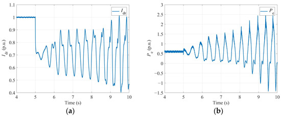
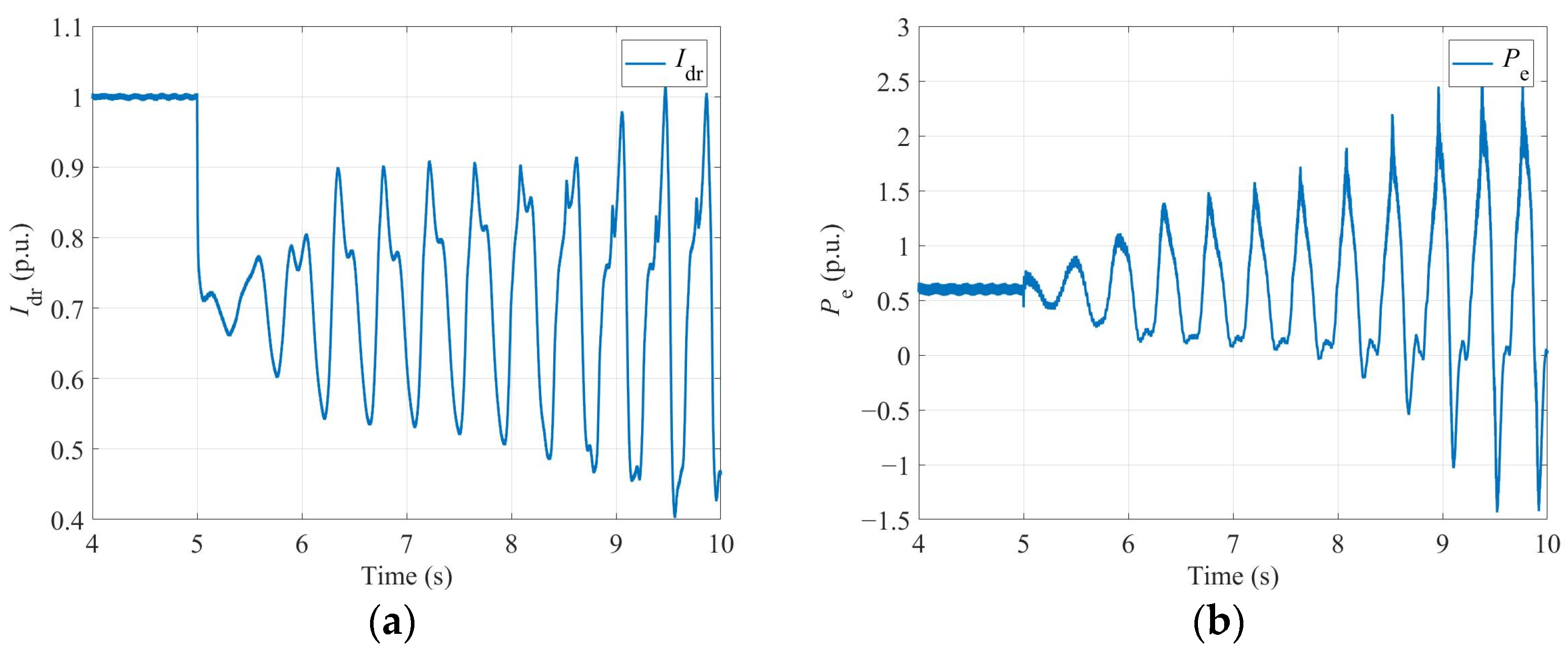
Under the parameter configuration shown in Table 2, the system’s tie-point voltage dropped to 0.4 pu at 5 s, causing the system to experience large-signal instability. The active power Pe of the VSG-DFIG and the DC current Idr of the LCC-HVDC are shown in Figure 16.
Table 2.
System Parameter Configuration Table 2.
Figure 16.
The physical waveform without any strategy applied. (a) Idr; (b) Pe.
Under the same parameter configuration, by incorporating the large signal stability enhancement strategy described in Section 4.3 for the output system, the physical waveforms of the system are shown in Figure 17.
Figure 17.
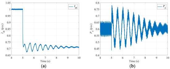
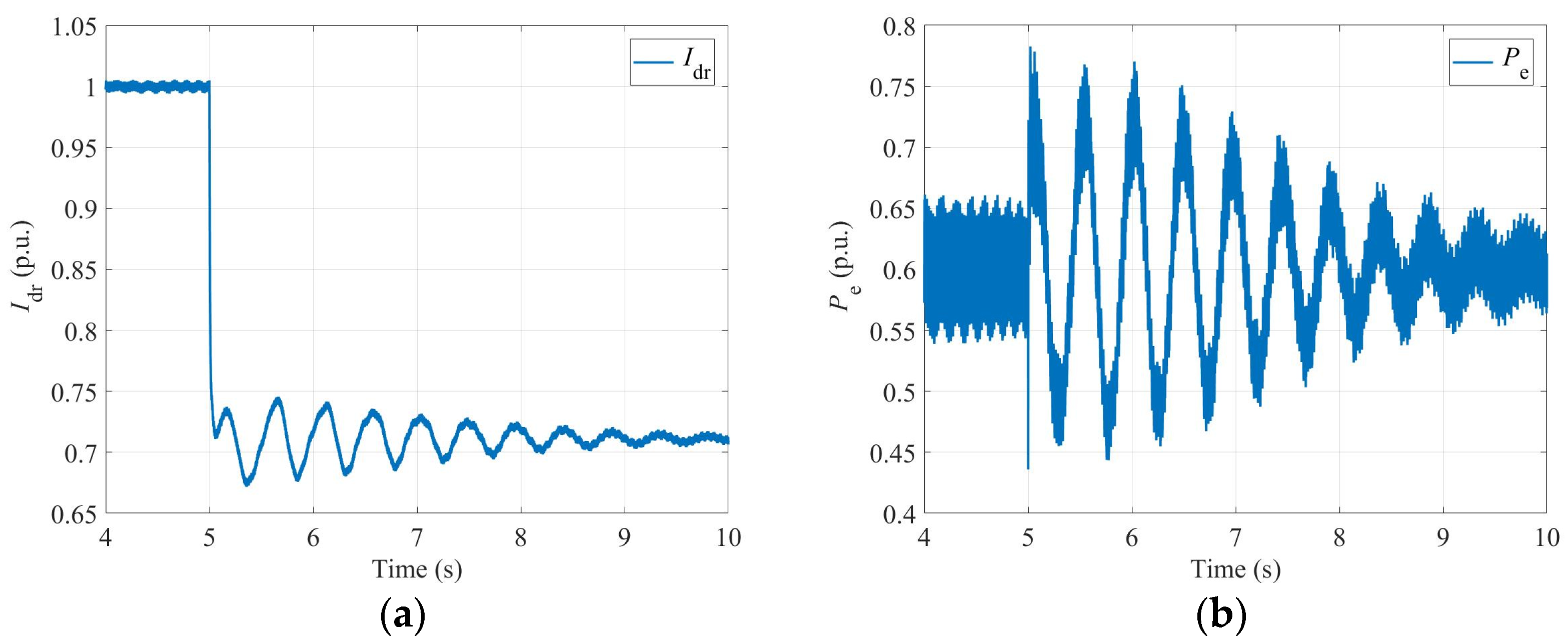
The physical waveform after the addition of the strategy. (a) Idr; (b) Pe.
By comparing Figure 17 with Figure 16, it can be seen that when the system is subjected to the same large disturbance impact, after adopting the additional virtual resistance strategy proposed in this paper, the system oscillation is effectively suppressed and can return to the steady-state operating point. However, the system without adding this strategy will experience instability. The results show that the proposed large-signal stability enhancement strategy based on virtual resistance can significantly improve the system’s tolerance to large disturbances and stability margin.
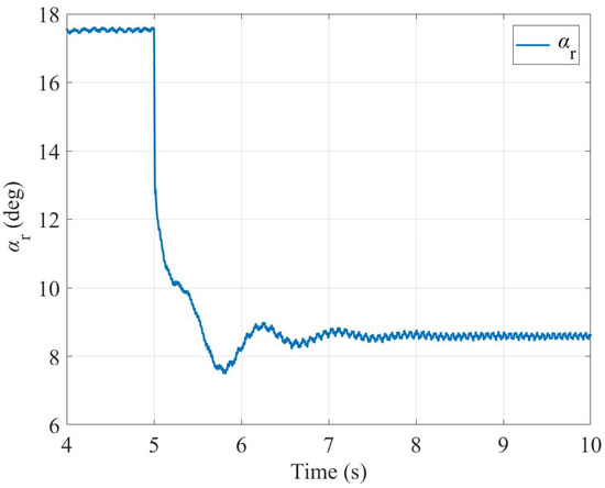
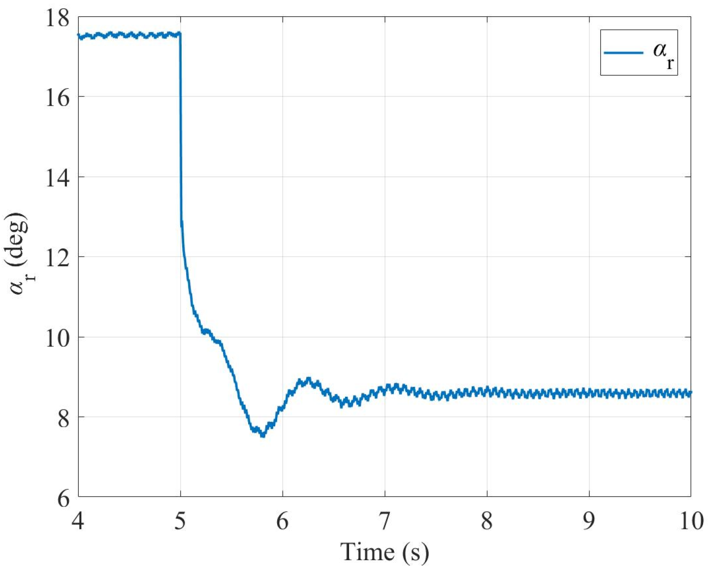
As shown in Figure 18 below, as well as in Figure 16 and Figure 17 above, the trigger angle waveforms of the working conditions discussed in this section are always within the operational boundaries of the commutation region, thereby confirming the physical rationality of the trajectory during the simulation process.
Figure 18.
Trigger angle waveform.
6. Conclusions
This paper investigates the large-signal stability of a grid-connected doubly fed induction generator (DFIG) system integrated with line-commutated converter high-voltage direct current (LCC-HVDC) transmission. Based on the mixed potential function theory, system modeling, stability analysis, and control enhancement are systematically conducted. The main conclusions are as follows:
- (1)
- By incorporating the physical dynamics and constant-current control dynamics of the LCC-HVDC sending-end rectifier station into a unified model, and utilizing the mathematical duality between PI controllers and RLC circuits, this paper virtually equates the dual-loop voltage and current control system of the VSG-DFIG to an RLC circuit. On this basis, an equivalent circuit model of the transmission system encompassing both control system and main circuit parameters is established, providing a solid foundation for subsequent stability analysis.
- (2)
- Based on the mixed potential function theory, the large-signal stability criterion of the system is derived. This criterion quantitatively reveals the influence of control parameters such as the proportional/integral coefficient of the voltage outer loop, the inertia/damping coefficient of VSG, the proportional coefficient of the current loop, and the proportional gain of the constant current control, as well as physical parameters such as line impedance and commutation reactance, on the stability boundary of the system. On this basis, a stability enhancement strategy of adding a virtual resistor in the LCC-HVDC control loop is proposed. This strategy does not require additional hardware equipment but can effectively suppress oscillations and prevent system instability under the same disturbance conditions by modifying the control loop. The theoretical criterion indicates that this strategy can introduce additional damping and effectively improve the large-signal stability margin.
- (3)
- The time-domain simulation results verify the correctness of the proposed theoretical criterion. The simulation analysis shows that increasing the proportional coefficient of the voltage outer loop, reducing the integral coefficient of the voltage outer loop, or increasing the proportional gain of the constant current control can accelerate the attenuation of oscillations after large disturbances and improve the stability margin, but at the same time, it will significantly exacerbate the steady-state harmonic distortion of the system, revealing the inherent contradiction of traditional parameter optimization strategies. The simulation results also verify the effectiveness of the virtual resistor strategy proposed in this paper in improving the system’s tolerance to large disturbances and stability margin.
Overall, this study provides a valuable theoretical foundation and technical reference for the parameter design, stability assessment, and operational control of wind farms integrated via LCC-HVDC transmission systems.
Author Contributions
Conceptualization, X.D.; Methodology, Y.L.; Software, Z.W.; Validation, L.Y.; Formal analysis, H.D.; Investigation, J.X.; Resources, Y.L.; Data curation, Z.W.; Writing—original draft, J.C.; Writing—review & editing, J.C.; Visualization, L.Y.; Supervision, J.X.; Project administration, H.D.; Funding acquisition, X.D. All authors have read and agreed to the published version of the manuscript.
Funding
This research was funded by Zhejiang Provincial Natural Science Foundation of China (No. LY23E070002), and Young Elite Scientist Sponsorship Program by Zhejiang Association for Science and Technology (No.ZJSKXQT2025039).
Data Availability Statement
All the data are available in the manuscript.
Conflicts of Interest
Author Haiming Du was employed by China Coal Xiyang Energy Co., Ltd. Baiyangling Coal Mine. The remaining authors declare that the research was conducted in the absence of any commercial or financial relationships that could be construed as a potential conflict of interest.
References
- Liu, H.; Yu, S.; Sun, D.; Wu, L.; Li, Y.; Wang, X. An Overview of Control Technologies and Principles for Grid-forming Converters. Proc. CSEE 2025, 45, 277–297. [Google Scholar]
- Zhan, C.; Wu, H.; Wang, X.; Tian, J.; Wang, X.; Lu, Y. An Overview of Stability Studies of Grid-forming Voltage Source Converters. Proc. CSEE 2023, 43, 2339–2359. [Google Scholar]
- Ke, S.; Yang, J.; Chen, L.; Fan, P.; Shi, X.; Li, G.; Wu, F. A Frequency Control Strategy for EV Stations Based on MPC-VSG in Islanded Microgrids. IEEE Trans. Ind. Inform. 2024, 20, 1819–1831. [Google Scholar] [CrossRef] [Scilit]
- Chen, S.; Sun, Y.; Hou, X.; Han, H.; Fu, S.; Su, M. Quantitative Parameters Design of VSG Oriented to Transient Synchronization Stability. IEEE Trans. Power Syst. 2023, 38, 4978–4981. [Google Scholar] [CrossRef] [Scilit]
- Li, G.; Song, W.; Liu, X. A Quasi-Harmonic Voltage Feedforward Control for Improving Power Quality in VSG-Based Islanded Microgrid. IEEE J. Emerg. Sel. Top. Power Electron. 2024, 12, 2994–3004. [Google Scholar] [CrossRef] [Scilit]
- Zhan, L.; Hu, B.; Chen, L.; Zhang, S.; Zhang, Z.; Nian, H. Transient Stability Analysis of Grid-Forming DFIG Equipped with Circular Current Limiter. IEEE Trans. Ind. Electron. 2025, 72, 11332–11336. [Google Scholar] [CrossRef] [Scilit]
- Liu, F.; Ruan, X.; Jiang, Y. Resonant Peak Suppression Approaches for Improving the Dynamic Performance of DCX-LLC Resonant Converter Based Two-Stage DC–DC Converter. IEEE Trans. Ind. Electron. 2023, 70, 5685–5695. [Google Scholar] [CrossRef] [Scilit]
- Zhan, L.; Hu, B.; Chen, L.; Liao, Y.; Li, M.; Nian, H. Transient stability enhancement of current limited-GFM inverters based on varying virtual impedance. IEEE Trans. Ind. Electron. 2024, 71, 15946–15958. [Google Scholar] [CrossRef] [Scilit]
- Gao, B.; Dong, X.; Sun, D.; Wu, L.; Wang, X.; Deng, X. Sub-synchronous Oscillation Characteristics and Mechanism Analysis ofMatching-control-based Grid-forming Direct Drive Wind Farm Transmitted Through LCC-HVDC System. Proc. CSEE 2024, 44, 9296–9310. [Google Scholar]
- Jiao, Y.; Nian, H. Grid-Forming Control for DFIG Based Wind Farms to Enhance the Stability of LCC-HVDC. IEEE Access 2020, 8, 156752–156762. [Google Scholar] [CrossRef] [Scilit]
- Li, H.; Hu, B.; Nian, H.; Liao, Y.; Xiong, L.; Liang, Z. Impedance Characteristic Analysis and Phase-Locked Angle Feedforward-Based Stability Improvement for LCC-HVDC in Sending AC Grid. IEEE Trans. Sustain. Energy 2025, 16, 588–600. [Google Scholar] [CrossRef] [Scilit]
- Zhao, W.; Li, H.; Xiong, F.; Nian, H.; Xu, J.; Liao, Y. Stability Analysis and Improvement for LCC-HVDC in Sending AC Grid with Wind Farms Based on Grid-Forming Energy Storage System. In Proceedings of the 2024 CPSS & IEEE International Symposium on Energy Storage and Conversion (ISESC), Xi’an, China; IEEE: New York, NY, USA, 2024; pp. 818–822. [Google Scholar]
- Nian, H.; Liu, Y.; Li, H.; Hu, B.; Liao, Y.; Yang, J. Commutation overlap characteristic modeling and stability analysis of LCC-HVDC in sending AC grid. IEEE Trans. Sustain. Energy 2022, 13, 1594–1606. [Google Scholar] [CrossRef] [Scilit]
- Zhen, Y.; Ju, M.; Gao, B.; Lu, W.; Liu, Y. Analysis of Sub-Synchronous Oscillation Characteristics and SuppressionStrategies of MC-PMSG Transmitted Through LCC-HVDC Systems. J. Electr. Eng. 2026, 41, 558–574. [Google Scholar]
- Yang, C.; Zhu, F.; Lu, N.; Yang, Y. Analysis on Uncertainty of Field-to-Wire Coupling Model in Time Domain. IEEE Trans. Power Deliv. 2022, 37, 3771–3781. [Google Scholar] [CrossRef] [Scilit]
- Yu, Z.; Chen, Z.; Zong, H.; Cai, X. A Transient Synchronization Stability Control Method With Global Stability for Renewable Power Plants Utilizing PLL-based Grid-following Converters. Proc. CSEE. 2026, 1–16. [Google Scholar] [CrossRef]
- Huang, S.; Fu, R.; Cao, G.; Hu, H.; Liang, D. Model Reference Adaptive Speed Control for Large-Stroke Bidirectional Linear Switched Reluctance Motor Based on Segmented Reference Model. Trans. China Electrotech. Soc. 2026, 41, 4011–4021. [Google Scholar]
- Wu, Z.; Han, H.; Liu, Z.; Su, M.; Sun, Y.; Zhang, X.; Wang, P. A Novel Method for Estimating the Region of Attraction for DC Microgrids via Brayton-Moser’s Mixed Potential Theory. IEEE Trans. Smart Grid 2023, 14, 3313–3316. [Google Scholar] [CrossRef] [Scilit]
- Liu, Z.; Ge, X.; Su, M.; Han, H.; Xiong, W.; Gui, Y. Complete Large-Signal Stability Analysis of DC Distribution Network via Brayton-Moser’s Mixed Potential Theory. IEEE Trans. Smart Grid 2023, 14, 866–877. [Google Scholar] [CrossRef] [Scilit]
- Liu, S.; Ning, J.; Xia, M.; Song, M.; Liu, X. Large-Signal Stability Analysis of Multimode Flexible Interconnected DC Microgrid Clusters. Trans. China Electrotech. Soc. 2026, 1–13. [Google Scholar] [CrossRef]
- Luo, D.; Zheng, H.; Yuan, X.; Tan, Z.; Zhang, C.; Tang, X.; Xu, Y. Large-signal stability analysis of DC microgrid based on virtual equivalent circuit model of controller. Power Syst. Technol. 2025, 49, 4729–4738. [Google Scholar]
- Wan, Z.; Xu, H.; Ge, P.; Yuan, X. Mixed potential function based large disturbance stabilityanalysis and enhancement strategy for MMC. Electr. Power Autom. Equip. 2025, 45, 124–132. [Google Scholar]
- Kan, P.; Zheng, H.; Yuan, X.; Xiong, W.; Wei, W.; Zhang, Y.; Cai, Y. Comparative Study on Impact of Different Models on Large Signal Stability Analysis Accuracy in MMC-HVDC Systems. Smart Power 2024, 52, 105–113. [Google Scholar]
- Yin, H.; Xu, Q.; Zhou, X.; Huang, X.; Wang, L.; Shuai, Z.; Guerrero, J.M. Large-Signal Stability Analysis of a Modular Multilevel Converter Based on Mixed Potential Theory. CSEE J. Power Energy Syst. 2025, 11, 1211–1225. [Google Scholar] [CrossRef] [Scilit]

Disclaimer/Publisher’s Note: The statements, opinions and data contained in all publications are solely those of the individual author(s) and contributor(s) and not of MDPI and/or the editor(s). MDPI and/or the editor(s) disclaim responsibility for any injury to people or property resulting from any ideas, methods, instructions or products referred to in the content. |
© 2026 by the authors. Licensee MDPI, Basel, Switzerland. This article is an open access article distributed under the terms and conditions of the Creative Commons Attribution (CC BY) license.