


Abstract
To improve renewable energy utilization and reduce fossil fuel consumption in building heating systems in Northwest China, this study proposes a solar–biogas hybrid heating system for the Jiuquan region. A dynamic simulation model was developed in TRNSYS, and multi-objective optimization was conducted using the NSGA-II algorithm. The optimization objectives were to maximize the solar fraction and minimize the initial system investment. The solar collector area, thermal storage tank volume, and biogas boiler start-up temperature were selected as decision variables. The results showed that the optimized solar fraction increased from 48.98% to 78.40% as the initial investment increased from 40,000 CNY to 80,000 CNY, although the marginal return gradually decreased. The NSGA-II algorithm generated a well-distributed Pareto front, revealing a clear trade-off between economic performance and solar energy utilization. Relative to the author-defined, proportionally scaled reference configurations, the optimized solutions increased the solar fraction by 18–21% across the examined investment levels. These improvement percentages are conditional on the adopted baseline definition. Considering both energy performance and economic feasibility, the scheme with a solar fraction of approximately 70% was identified as the compromise solution. Compared with the initial design, this scheme increased the initial investment by 15.52% and improved the solar fraction by 20.69%. These results indicate that appropriate configuration of key system parameters can substantially enhance renewable energy utilization. The proposed optimization method provides a useful reference for the design and operation of solar–biogas hybrid heating systems in Northwest China.
1. Introduction
Space heating is a major component of operational energy consumption in buildings located in cold regions and contributes substantially to total building energy use and carbon emissions [1,2]. In the context of China’s dual-carbon goals and the growing demand for energy conservation and emission reduction in the building sector, efficient and clean heating technologies based on renewable energy have become an important research priority. Solar energy is clean and abundant but inherently intermittent [3,4]. Nevertheless, in the field of building heating, the utilization of solar energy still offers considerable potential for energy savings and emission reductions. The use of solar energy for space heating can effectively reduce dependence on conventional fossil fuels, lower greenhouse gas emissions, and promote the transition of building energy systems towards low-carbon pathways.
Solar heating systems have attracted considerable research attention in recent years. To address the intermittency and variability of solar resources, previous studies have focused on improving collector performance, optimizing thermal storage technologies, and developing advanced control strategies [5,6]. The integration of solar collectors with thermal storage devices can partially mitigate the adverse effects of solar radiation fluctuations and improve solar energy utilization [7]. Consequently, stand-alone solar heating systems may fail to meet continuous building heating demand during periods of insufficient irradiation, making auxiliary heat sources necessary [8,9]. Multi-energy complementary heating systems have therefore become an important technical pathway for improving the reliability of solar heating systems [10].
Hybrid heating systems combining solar energy with auxiliary heat sources, such as air-source heat pumps, electric boilers, and biomass boilers, have been widely investigated [11]. Proper integration of auxiliary heat sources can compensate for the intermittency of solar energy and enhance heating reliability. Among the available renewable options, biomass is characterized by abundant resources, convenient storage, and strong dispatchability [12]. Biogas, produced through anaerobic digestion and composed mainly of methane, can provide stable and controllable heat through combustion. Its dispatchability complements the intermittent nature of solar energy, making a solar–biogas configuration suitable for renewable heating applications.
Previous studies have investigated solar–biomass hybrid heating systems from several perspectives, including system configuration, operational performance, and economic feasibility. For example, dynamic simulation models have been used to evaluate the effects of individual design parameters, such as collector area and thermal storage capacity, on system performance. Life-cycle cost analysis has also been applied to assess economic feasibility, while intelligent control strategies have been developed to coordinate multiple heat sources. However, for rural heating applications in Jiuquan, the initial capital requirement is also a decision-relevant indicator because it directly affects the upfront affordability and near-term feasibility of system adoption. Therefore, this study focuses on the trade-off between initial investment and solar-energy utilization. This choice is intended to represent the capital-entry requirement rather than the complete lifecycle economic performance of the system. Nevertheless, these studies have generally examined specific parameters or operational aspects separately. The coordinated optimization of multiple key parameters in solar–biogas hybrid heating systems, particularly with respect to the trade-off between solar energy utilization and initial investment, remains insufficiently explored. Increasing the solar fraction generally requires larger collector areas and greater thermal storage capacities, which increases capital cost. Identifying an appropriate balance between economic performance and renewable energy utilization is therefore a key issue for the practical application of solar–biogas hybrid heating systems.
Multi-objective optimization methods have been widely applied to the design and operation of energy systems [13,14,15]. Among them, the Non-Dominated Sorting Genetic Algorithm II (NSGA-II) is commonly used in building energy system optimization because of its global search capability, convergence performance, and capacity to handle multiple conflicting objectives simultaneously [16,17]. By generating a Pareto-optimal solution set, NSGA-II can reveal trade-offs among competing objectives and provide a quantitative basis for system design decisions.
Recent studies have investigated solar–biogas heating systems from different perspectives. Liu et al. [18] evaluated the thermal characteristics and heat-storage role of a solar–biogas heating system for buildings. Sun et al. [19] developed a TRNSYS model of a solar-assisted biogas and air-source heat-pump system for rural heating and employed NSGA-II for bi-objective optimization. However, the joint optimization of collector area, storage-tank volume, and biogas-boiler control temperature for a solar–biogas heating system under the climatic and building-load conditions of Jiuquan remains insufficiently investigated.
2. Climatic Characteristics of Jiuquan Area
Jiuquan, located in the western Hexi Corridor of Gansu Province, has an arid and semi-arid climate and possesses abundant solar energy resources, providing favorable conditions for solar heating applications. Its rural areas also contain substantial agricultural and livestock residues, which provide a potential resource basis for biogas production [20]. Given the marked regional differences in climate and solar resource distribution across Gansu Province, Jiuquan was selected specifically to represent the solar-rich conditions of the western Hexi Corridor. Therefore, the development of solar–biogas hybrid heating systems in Jiuquan offers both resource advantages and practical engineering relevance.
On this basis, this study selected a typical building in Jiuquan as the research object and developed a dynamic simulation model of a solar–biogas hybrid heating system [20]. Mathematical models of the main components, including solar collectors, the thermal storage tank, and the biogas boiler, were established, and system operation was analyzed using TRNSYS. The NSGA-II algorithm was then used for multi-objective optimization and to obtain the Pareto-optimal solution set. The variation characteristics of key system parameters were further examined, and a compromise solution balancing economic performance and renewable energy utilization was identified. The findings provide theoretical support for the design and application of solar–biogas hybrid heating systems in Northwest China.
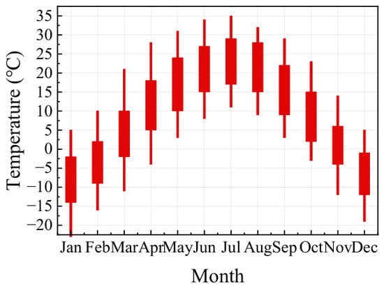
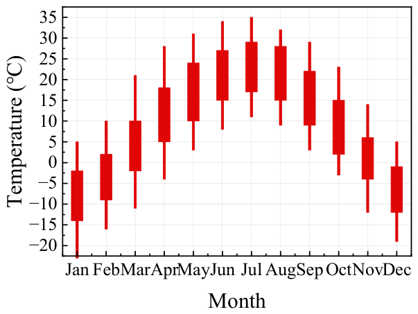
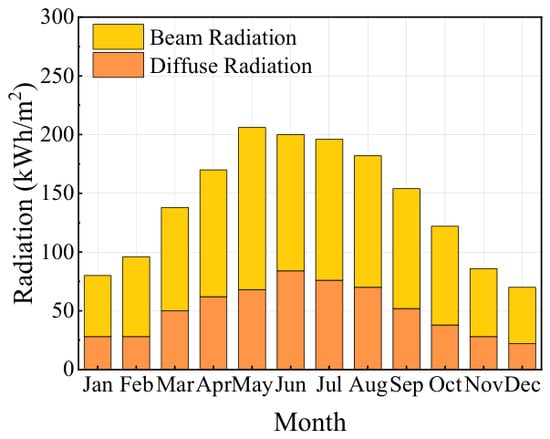
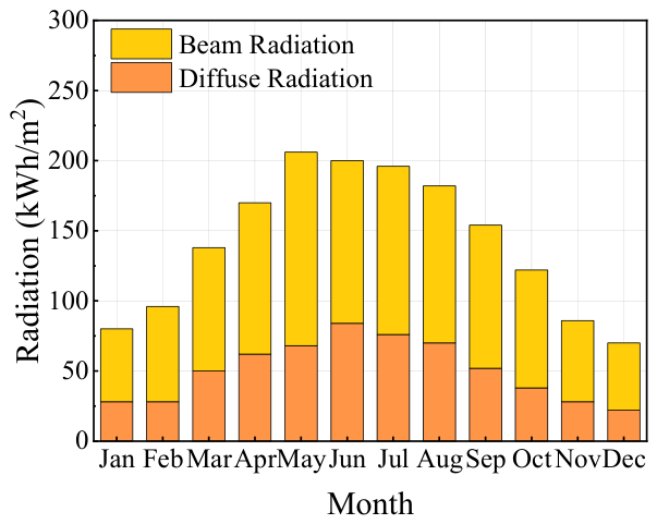
The monthly average air temperature and monthly average solar radiation data for this region were analyzed to characterize annual temperature variation and the seasonal distribution of solar energy resources in Jiuquan. The results are presented in Figure 1 and Figure 2.
Figure 1.
Distribution characteristics of monthly air temperature.
Figure 2.
Monthly distributions of solar radiation.
For each month shown in Figure 1, the filled red bar represents the interval between the monthly mean daily minimum and maximum temperatures. The lower and upper vertical ranges extend to the monthly extreme minimum and maximum temperatures, respectively. The monthly temperature variations in Jiuquan show that this city has a distinct unimodal annual pattern, with the lowest temperatures occurring in January, and the highest temperatures occurring in July. This pattern is consistent with the characteristics of a temperate continental climate. In Jiuquan, winter temperatures are relatively low; the average minimum temperature in January approaches −15 °C, and extreme minimum temperatures fall below −20 °C. In summer, the average maximum temperature in July approaches 30 °C, while extreme maximum temperatures exceed 35 °C. The annual temperature difference is substantial, reaching nearly 50 °C, which indicates the strong continental and arid-cold climatic characteristics of the region.
A combined analysis of temperature and solar radiation data shows that Jiuquan is characterized by cold winters and abundant solar energy resources. The region experiences substantial heating demand from December to February while maintaining considerable solar radiation, providing favorable climatic conditions for solar heating applications. Its low winter temperatures and high solar resource availability make it suitable for investigating high-solar-fraction heating systems. Accordingly, this study uses the meteorological conditions of Jiuquan as the sole climatic boundary for the building-load simulation and the subsequent TRNSYS-based optimization of the solar–biogas hybrid heating system. The conclusions are therefore specific to the selected rural residential building in Jiuquan and may apply only to regions with comparable climatic and building-load conditions.
3. Building Load Characteristics During the Heating Season in Jiuquan
3.1. Determination of Hourly Outdoor Temperature and Solar Radiation Intensity During the Heating Season
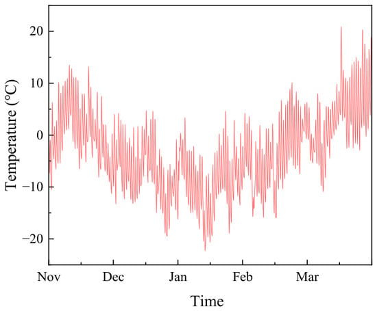
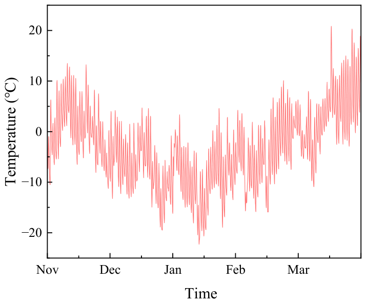
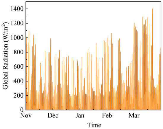
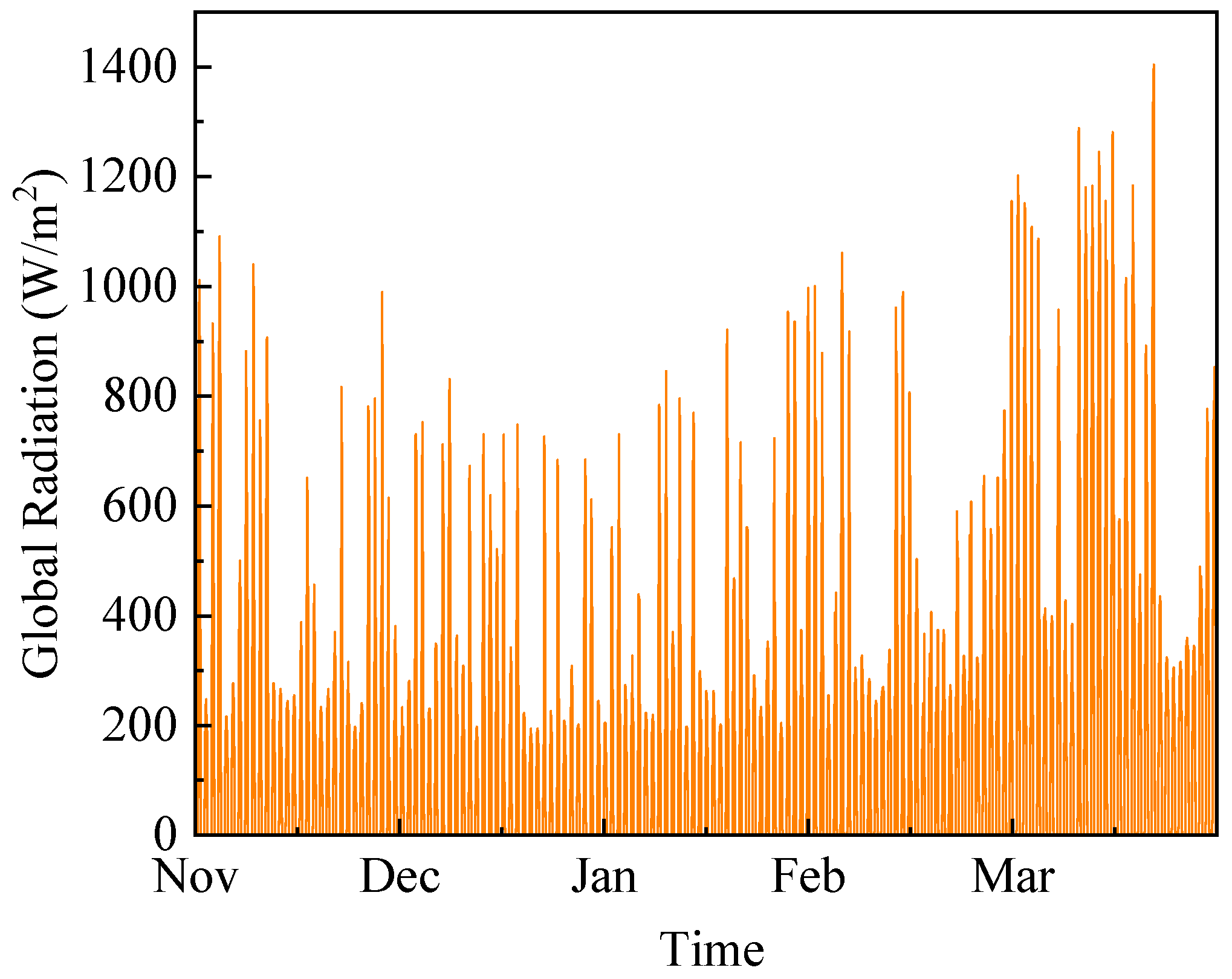
Based on the Typical Meteorological Year (TMY) data for Jiuquan obtained from Meteonorm, hourly meteorological parameters, including dry-bulb temperature, solar radiation, wind speed, and relative humidity, were collected. Figure 3 and Figure 4 show the hourly dry-bulb temperature and solar radiation intensity during the heating season in Jiuquan, respectively. The weather data file was then imported into TRNSYS to establish the building thermal model. Hourly building heating loads throughout the heating season were subsequently simulated and analyzed, providing fundamental data for the design of building-integrated solar heating systems and the configuration of hybrid renewable energy supply systems.
Figure 3.
Hourly dry-bulb temperature in Jiuquan during the heating season.
Figure 4.
Hourly solar radiation in Jiuquan during the heating season.
The hourly meteorological dataset adopted in this study is the Typical Meteorological Year (TMY) generated by Meteonorm v8.0. The geographic information of the Jiuquan study site is as follows: latitude 39.74° N, longitude 98.50° E, altitude 1170 m above sea level, UTC+8 China Standard Time. The meteorological data covers multi-year average climate records from 2010 to 2020. The evacuated tube solar collector is arranged with a tilt angle of 40° and an azimuth angle of 0° (due south). The dynamic TRNSYS simulation started at 0:00 on November 1 and ended at 24:00 on March 31 of the next year, with an hourly calculation time step.
3.2. Determination of Building Envelope Parameters
After the meteorological data file was obtained, a building thermal model was established to represent the climatic characteristics of Jiuquan and calculate the building heating load. The building envelope is a key factor affecting heat loss and heating energy consumption, and its thermal performance directly determines the insulation level and heating demand of the building. Therefore, the exterior walls, interior walls, roof, floor, and external windows were modeled in detail in TRNSYS.
As a result, the heating demand remains substantial throughout winter. To reduce heat loss through the envelope and improve thermal insulation performance, expanded polystyrene (EPS) insulation layers were added to the exterior walls and roof. The representative building is selected strictly following local rural building energy-saving codes, adopting mainstream layout and widely-used envelope structures, including double-glazed windows that balance thermal performance and rural construction costs in Jiuquan’s severe cold climate [21]. The target rural building is a single-story rectangular residence with a total conditioned floor area of 120 m2, length of 15 m, eave height of 3.2 m and width of 8 m. The primary orientation of the building is south. The gross area of the four exterior walls is 2(15 + 8) × 3.2 = 147.2 m2, and the total exterior-window area is 16.8 m2. Therefore, the overall window-to-wall ratio, calculated using the gross area of all four exterior walls, is 16.8/147.2 = 0.114, or approximately 0.11. The entire house is defined as a single unified thermal zone, without separate temperature control partitions, and the standard household occupancy is set to five people, consistent with local rural living habits. The overall seasonal heating demand of the whole building is 15,444 kWh, and the peak heating load reaches 16.4 kW (136.7 W/m2). The construction assemblies and thermal properties of each envelope component were determined according to current building energy-efficiency design standards. The construction details and thermal performance parameters are listed in Table 1 [22].
Table 1.
Thermal performance parameters of the building envelope.
3.3. Determination of Internal Heat Gains
In TRNBuild, in addition to meteorological boundary conditions and envelope thermal properties, internal heat gain parameters must be specified, including heat gains from occupants, lighting, equipment, and fresh air ventilation. Internal heat gains affect both the indoor thermal environment and the calculated building heating load. These parameters were therefore determined based on the actual use conditions of the building.
According to the Design Code for Heating Ventilation and Air Conditioning of Civil Buildings and the Energy Efficiency Design Standard for Rural Residential Buildings, the indoor design temperature for residential buildings under winter heating conditions is generally 18–20 °C. Considering the cold winter climate and substantial heating demand in Jiuquan, as well as the balance between thermal comfort and energy efficiency, the indoor design temperature was set to 18 °C. Based on current building energy-efficiency standards and typical occupancy characteristics of rural residential buildings, the occupant density was assumed to be 0.04 persons/m2, with a sensible heat gain of 75 W per person. The lighting power density was set to 5 W/m2, and the power density of household appliances and other equipment was set to 3 W/m2. To satisfy indoor air quality requirements, the fresh air ventilation rate was specified as 30 m3/(h·person). These internal heat gain parameters were used as input conditions for the TRNSYS building thermal model to calculate the hourly heating load throughout the heating season and to support the capacity design of the building-integrated solar heating system.
3.4. Analysis of Building Load Simulation Results During the Heating Season
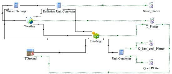
After the physical building model was defined in TRNBuild and the envelope and internal heat gain parameters were specified, the dynamic building load model was established. The resulting model is shown in Figure 5 (The solid line represents the physical connection relationship between model components, while the dashed line represents the relationship between simulation data transmission and result output.).
Figure 5.
Building load simulation model.
To verify the rationality of the established TRNSYS building model, the simulated seasonal heating load per unit area is compared with national design standards and peer measured data for rural buildings in Jiuquan, as shown below.
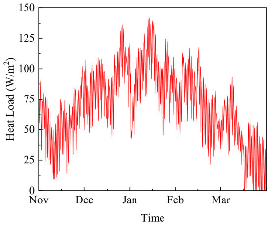
The simulated seasonal heating load of the target rural building is 128.7 kWh/m2. According to GB/T 50824 [23], Design Standard for Energy Efficiency of Rural Residential Buildings in Severe Cold and Cold Zones, the standard seasonal heating load range for unrenovated rural houses in Hexi Corridor severe cold regions is 120–135 kWh/m2. Previous field investigations of rural dwellings in the Hexi Corridor, including Jiuquan, have documented poor winter indoor thermal conditions and substantial space-heating demand [24,25]. The simulated seasonal heating demand of 128.7 kWh/m2 is therefore considered physically plausible for the regional climate and building characteristics. However, because building-specific measured heating-consumption data are unavailable, this comparison is regarded as a plausibility assessment rather than as a direct experimental validation. Our simulated value falls within both the standard interval and the literature measured range, which demonstrates that the building envelope, internal heat gain and meteorological boundary settings are reasonable, and the building load simulation results are credible for subsequent optimization. After the parameter settings were completed, the dynamic building load simulation was performed to obtain the hourly heating load of the building throughout the heating season. The simulation results are presented in Figure 6.
Figure 6.
Hourly heating load of the building during the heating season in Jiuquan.
Figure 6 presents the hourly heating load of the studied building throughout the heating season in Jiuquan. The heating load varies synchronously with outdoor temperature: it starts relatively low in November, rises gradually to a peak value of approximately 140 W/m2 during January–February, and declines continuously until the end of March. The heating load is mainly distributed within 50–100 W/m2 for most of the heating period. The frequent periodic fluctuations on the curve are dominated by diurnal changes in outdoor temperature and solar irradiance, reflecting their direct impacts on instantaneous building heating demand. To further quantitatively validate the reliability of the TRNSYS building and heating system model, the simulated seasonal heating load per unit area (128.7 kWh/m2) is compared with published field measurement data of Jiuquan rural buildings (124–132 kWh/m2) and the GB/T 50824 standard range (120–135 kWh/m2). Taking the average measured load of 128 kWh/m2 as the reference value, the relative error of simulation results is calculated as
where:
: simulated seasonal heating load, kWh;
: average field-measured heating load from the literature, kWh.
The calculated relative error is only 0.55%, which falls within the commonly accepted engineering tolerance (±5%). It should be noted that the ZDT benchmark-function tests reported in the Supplementary Material evaluate only the convergence and distribution performance of the NSGA-II algorithm. In contrast, the comparison between the simulated seasonal heating load and the field-measured data, together with the relative-error calculation presented above, provides an independent validation of the physical TRNSYS building model. The validation performed in this study is limited to the building thermal-load model. This comparison supports the reliability of the building heating-load boundary used in the coupled simulation. However, it does not represent experimental validation of the complete solar–biogas heating system. The collector, storage tank, circulation loop, controller, and auxiliary boiler were modeled using established component equations and manufacturer or literature parameters, and their interactions were checked through hourly energy balances.
4. Establishment of the TRNSYS Simulation Model of the System
4.1. Solar–Biogas Heating System
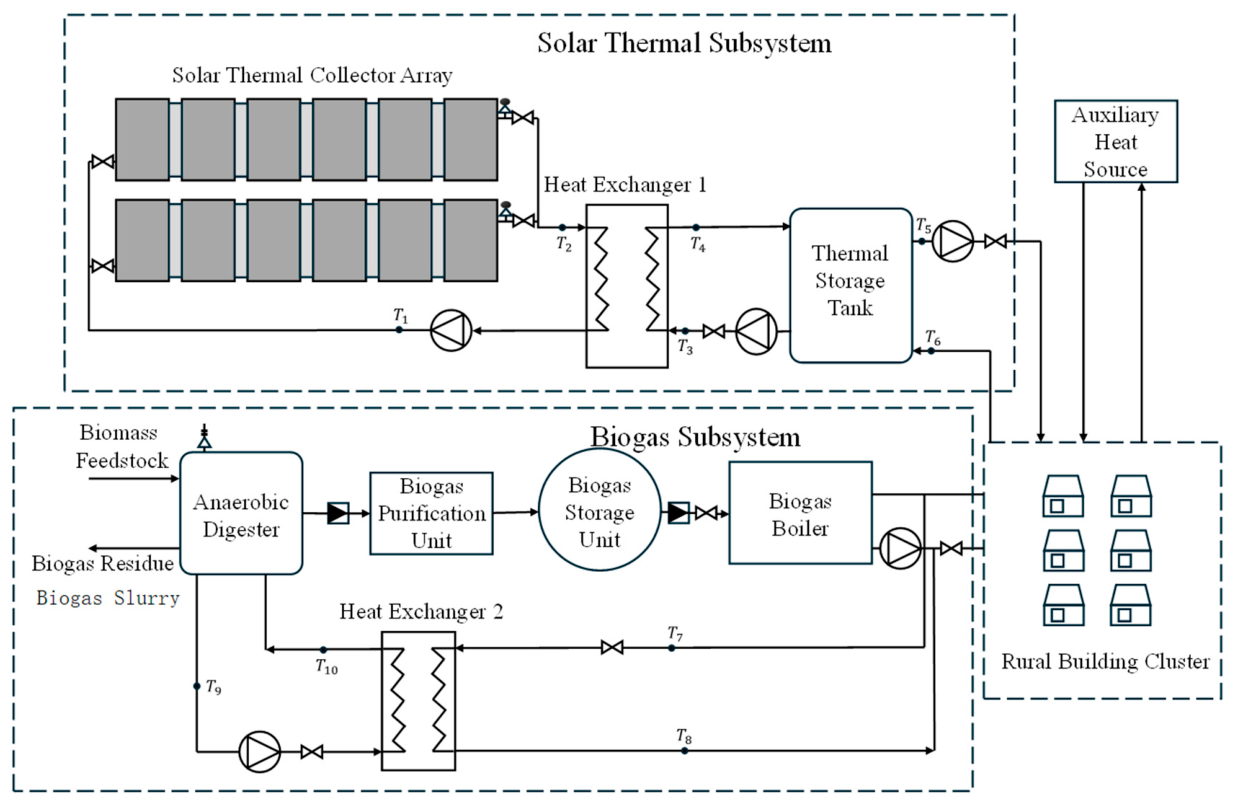
Considering the local availability of solar and biomass resources, a solar–biogas heating system is proposed for the selected rural building in Jiuquan. Solar energy is used as the primary heat source, while a biogas-fired boiler serves as the auxiliary heat source. The conceptual system configuration and the TRNSYS simulation boundary are presented in Figure 7.
Figure 7.
Conceptual configuration of the complete solar–biogas heating system and the boundary of the TRNSYS-simulated heating subsystem.
Figure 7 presents the conceptual configuration of the complete solar–biogas heating system. The upstream biogas-production chain, including the anaerobic digester, purification unit, and gas-storage unit, is shown only to illustrate the potential fuel-supply pathway and is not included in the TRNSYS simulation. The actual simulation boundary begins at the idealized biogas-fired auxiliary boiler and includes the solar collector array, thermal storage tank, circulation pumps, controllers, heat exchangers, building-load model, and heating terminal. The solar collectors serve as the primary heat source by converting solar radiation into thermal energy. The thermal storage tank stores heat generated by the solar collection system and balances the mismatch between heat supply and heating demand. The biogas boiler serves as an auxiliary heat source and supplies additional thermal energy when solar heat is insufficient, thereby ensuring continuous and stable building heating.
The system operates according to a solar-priority control strategy. Under sufficient solar radiation, the collected heat is transferred through the collector loop to the thermal storage tank and subsequently supplied to the building through the heating loop. When the tank temperature falls below a preset threshold or the available solar heat cannot satisfy the building load, the biogas boiler is activated. This coordinated operation mitigates solar intermittency and ensures a stable heat supply while maintaining a high share of renewable energy.
4.2. Mathematical Models of the Main System Components
To characterize the operating behavior and energy performance of the system, mathematical models of the main components were established. In this study, a simulation-based approach was used to analyze dynamic system operation. The component models were implemented mainly through TRNSYS modules, providing the theoretical basis for the subsequent system simulations.
Solar collector model: In TRNSYS, Type 71 was selected to represent the solar collector. This model uses the Hottel–Whillier equation to describe collector thermal performance. The collector efficiency (η), which characterizes the heat collection performance of the solar collector, is defined as follows:
where:
η: thermal efficiency of the evacuated-tube solar collector;
m: mass flow rate of the heat transfer fluid, kg/s;
cp: specific heat capacity of the heat transfer fluid at constant pressure, kJ/(kg·°C);
To and Ti: outlet and inlet temperatures of the heat transfer fluid, °C;
A: collector area, m2;
IT: total solar radiation incident on the tilted collector surface, W/m2;
FR: heat removal factor;
(τα)n: product of cover transmittance and absorber absorptance under normal solar incidence;
UL: overall heat loss coefficient per unit collector area, W/(m2·°C);
Ta: ambient air temperature, °C;
ULT: heat loss coefficient associated with changes in ambient temperature, W/(m2·°C).
Equation (2) can be further simplified as follows:
where:
ΔT: temperature difference between the inlet fluid temperature and the ambient air temperature, °C;
a0, a1, and a2: performance coefficients of the standard quadratic efficiency equation. The quadratic efficiency coefficients are , .
The thermal efficiency of the evacuated-tube solar collector was calculated using the standard quadratic efficiency model. The model form follows the conventional collector-performance formulation described by Duffie and Beckman. The coefficients were obtained from the certified performance data of the selected evacuated-tube collector. These coefficients were entered as fixed collector-performance parameters in the TRNSYS model.
Biogas boiler model: Within the TRNSYS simulation boundary, the biogas subsystem is represented solely by an idealized auxiliary boiler with a sufficient and continuous fuel supply. The production, purification, and storage of biogas are not dynamically modeled. When the solar collector and thermal storage tank cannot satisfy the building heating demand, the boiler converts the prescribed biogas fuel input into useful thermal energy according to its thermal efficiency. Its useful heat output is expressed as follows:
where:
Qb: useful heat output of the biogas boiler, kW;
ηb: thermal efficiency of the biogas boiler;
Vb: biogas consumption rate, m3/h;
Hb: lower heating value of biogas, MJ/m3.
All fixed biogas and boiler thermal parameters adopted in Equation (4) are listed in Table 2 for reference.
Table 2.
Thermal characteristic parameters of biogas and the biogas boiler.
All geometry, equipment, and control parameters used in the TRNSYS dynamic simulation are fully listed in the model in Table 3.
Table 3.
Consolidated TRNSYS simulation parameters.
4.3. Establishment of the Simulation Model of the Solar–Biogas Hybrid Heating System
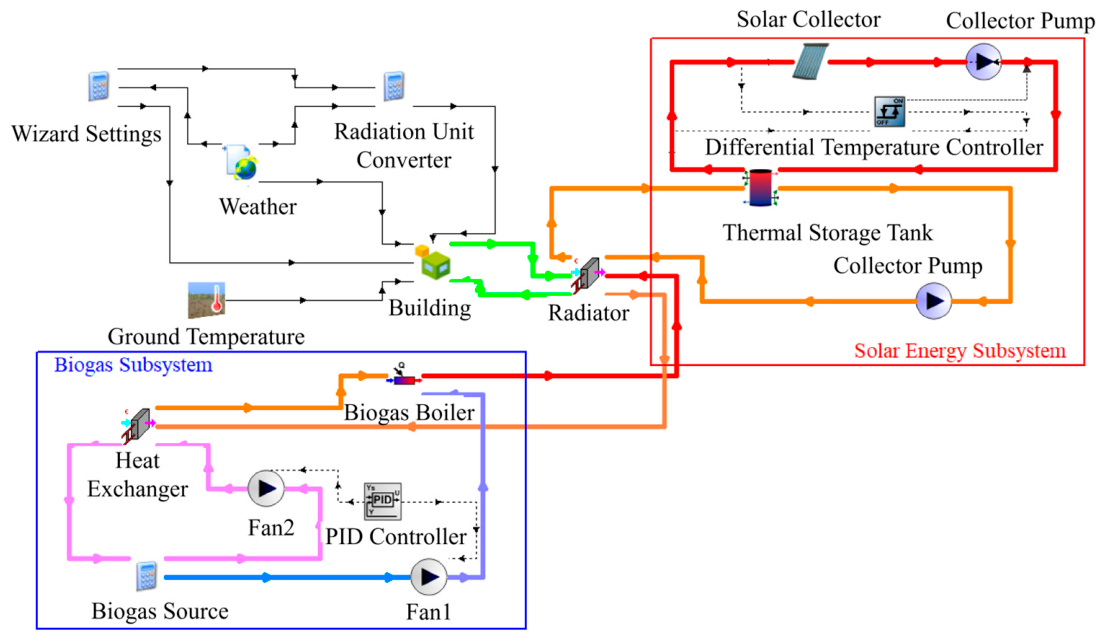
The TRNSYS model was established strictly within the simulation boundary defined in Figure 7. It includes the weather-data reader, solar collector array, differential-temperature controller, circulation pumps, stratified thermal storage tank, idealized biogas-fired auxiliary boiler, PID controller, building-load model, and heating terminal. The anaerobic digester, biogas-purification unit, gas-storage unit, and digester-heating loop were excluded from the TRNSYS model, energy balance, equipment-sizing analysis, and investment calculation. A sufficient and continuous biogas supply was assumed without seasonal production constraints. Accordingly, Figure 8 presents only the components actually implemented in TRNSYS (The different colored pipelines in the figure represent different forms of energy transfer processes, where red represents the solar collection cycle, orange represents the hot water distribution circuit, blue represents the biogas supply circuit, green represents the building side heat exchange process, and black represents the control and information transmission path.), and Table 4 lists their corresponding component types and parameters.
Figure 8.
TRNSYS model of the simulated solar heating system assisted by an idealized biogas-fired boiler.
Table 4.
Full list of TRNSYS component modules and core parameters.
The auxiliary boiler capacity was not treated as an optimization variable. To ensure full backup heating under design conditions, the boiler was sized using a capacity factor of 1.5 applied to the simulated peak building load of 16.4 kW. The calculated capacity was 24.6 kW, and a commercially available 25 kW boiler was therefore selected. The same 25 kW boiler was retained for every Pareto solution; optimization changes its operating duration and annual fuel consumption, but not its rated capacity.
In this study, the solar–biogas hybrid heating system was modeled in TRNSYS 18 with a simulation time step of 1 h. During system operation, different control strategies were adopted for the solar heating loop and the biogas auxiliary heating loop to ensure stable and efficient performance.
For the solar thermal subsystem, a differential temperature controller was used to regulate the collector circulation loop. The controller monitors the temperature difference between the collector outlet and the bottom of the thermal storage tank and compares it with predefined upper and lower dead-band limits. When the temperature difference exceeds the upper dead-band value, the controller starts the circulation pump, allowing the heat collected by the solar collectors to be transferred to the thermal storage tank. When the temperature difference falls below the lower dead-band value, the controller stops the circulation pump, preventing heat loss caused by circulating low-temperature working fluid.
For the biogas auxiliary-heating subsystem, the controller monitors the upper-layer temperature of the thermal storage tank. The biogas boiler is activated when the monitored temperature falls below the prescribed start-up temperature . If the upper-tank temperature profile remains unchanged, increasing causes the boiler to activate earlier because the monitored temperature reaches the higher threshold sooner during cooling. Conversely, when the monitored tank temperature reaches or exceeds the prescribed control limit, the controller reduces the boiler output or switches the boiler off. In the Pareto-optimal solutions, changes in occur together with changes in collector area and storage-tank volume. Consequently, boiler operating time must be interpreted as the combined result of these parameters and cannot be attributed to alone.
5. Optimization Study of the Solar–Biogas Hybrid Heating System
5.1. Selection and Validation of the Optimization Algorithm
The performance of the solar–biogas hybrid heating system is jointly affected by several parameters, including solar collector area, thermal storage tank volume, and boiler control settings. A multi-objective optimization approach was therefore adopted to determine the optimal configuration of these key parameters.
NSGA-II was selected because its fast non-dominated sorting and crowding-distance mechanisms promote convergence while maintaining solution diversity in conflicting multi-objective problems [27]. It was used to optimize the system parameters and generate a well-distributed Pareto front, revealing the trade-off between solar energy utilization and initial investment.
5.2. Determination of Objective Functions and Decision Variables
Based on the building heating load simulation for Jiuquan and the established solar–biogas hybrid heating system model, the key system parameters were optimized to improve renewable energy utilization and reduce initial investment. Because the solar collector area, thermal storage tank volume, and boiler control temperature directly affect system performance and equipment cost, the collector area (A_c), storage tank volume (Vt), and biogas boiler start-up temperature (Tset) were selected as decision variables for multi-objective optimization [28].
In this study, the solar fraction and total initial investment cost were selected as the optimization objectives. The solar fraction represents the proportion of the building heating load supplied by solar energy and was maximized to enhance renewable energy utilization. Total initial investment includes the purchase and installation costs of solar collectors, thermal storage tanks, and related auxiliary equipment and was minimized to improve economic feasibility. In this context, initial investment is used to represent the upfront affordability of system deployment; it is not intended as a substitute for lifecycle-cost assessment. The objective functions are expressed as follows:
Ac: solar collector area, m2;
Vt: thermal storage-tank volume, m3;
Tset: start-up temperature of the auxiliary biogas boiler, °C;
: unbounded solar-fraction response calculated using the algebraic response function, dimensionless;
: bounded solar fraction, constrained to the physical interval, dimensionless;
: first objective function to be minimized; minimizing is equivalent to maximizing the solar fraction;
: second objective function to be minimized, representing the total initial investment, CNY;
: total initial investment of the system, CNY;
: installed cost of the solar collector system, CNY;
: investment cost of the thermal storage tank, CNY;
: fixed lump-sum investment cost of the auxiliary biogas boiler and associated equipment, CNY.
where:
: solar collector unit cost (CNY/m2);
: heat storage tank unit cost (CNY/m3). The quoted prices correspond to the same base year and include the cost items specified in Table 5.
Table 5.
Economic parameters for initial investment calculation.
The multi-objective optimization problem can therefore be formulated as follows:
where the decision variables are defined as follows:
The unit investment coefficients are derived from the average market price level of Jiuquan’s local heating projects [18,26].
5.3. Constraints
To ensure that the optimization results satisfy the practical operating requirements of the system, the following constraints were imposed: the building heating load satisfaction rate should not be lower than 95%; the indoor temperature during the heating season should be maintained within 18–20 °C; the solar collector area should be limited to 20–80 m2; the thermal storage tank volume should be constrained within 0.5–3.0 m3; and the biogas boiler start-up temperature should be restricted to 35–50 °C. Under the premise of thermal comfort and stable system operation, the multi-objective optimization method was applied to obtain the optimal parameter configuration and to provide a theoretical basis for the design of solar–biogas hybrid heating systems in Gansu Province. The decision-variable constraints are defined as follows:
where:
ηh is the heating load satisfaction rate, defined as the ratio of the number of hours during the heating season when the indoor temperature reaches the design temperature (18 °C) to the total heating season hours;
Tin is the indoor temperature during the heating season, °C;
: total hours with an indoor temperature ≥ 18 °C;
: total heating-season hourly steps.
The 95% threshold is a mandatory thermal comfort limit. Static penalty function is adopted. A large constant M = 100 is added to both objectives for any solution with . Infeasible individuals are eliminated during sorting; variable repair is not used.
To enforce the heating load satisfaction rate constraint during the NSGA-II optimization, a penalty function method is adopted. Any solution that fails to meet the ηh ≥ 95% criterion will have its objective function values penalized, thereby guiding the search towards the feasible region. The upper limit of 80 m2 for the solar collector area is set to match the extreme heating load demand of the building, fit the maximum installable roof space of local rural houses [10], and ensure that the Pareto front covers high solar-fraction optimization schemes [19].
After defining variable constraints and penalty rules, the hyperparameters of NSGA-II used for practical system optimization are specified as population size = 100, maximum iterations = 500, crossover probability = 0.9, and mutation probability = 0.1.
The parameter difference from those in the Supplementary Material (population 150, iterations 200) arises from distinct calculation loads. The analysis in the Supplementary Material only tests standard mathematical test functions, without TRNSYS co-simulation, so a larger population and fewer iterations are adopted for fast comparison. For this solar–biogas coupled system, each individual requires a full heating-season dynamic simulation with heavy computation; population size is reduced to cut total simulation cost, while iterations are raised to guarantee full Pareto convergence under a smaller population.
For parameter rationality:
(1) Crossover probability = 0.9. A high crossover rate facilitates gene exchange of elite continuous variables (collector area, tank volume, boiler temperature), rapidly excavating balanced solutions between the initial cost and solar fraction.
(2) Mutation probability = 0.1. Moderate perturbation prevents premature local convergence and maintains population diversity, without destroying high-performance candidate solutions.
This parameter set balances computational burden, convergence precision and solution diversity for the co-simulation optimization problem.
5.4. Pareto Front Analysis
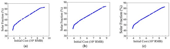
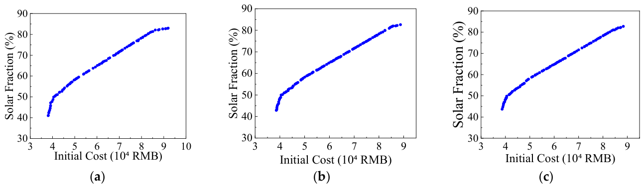
During optimization, an initial population satisfying all constraints was randomly generated. Through selection, crossover, and mutation, the population was iteratively updated until convergence, yielding the Pareto-optimal solution set for the system (Figure 9).
Figure 9.
Evolution of the Pareto front at different numbers of iterations. (a) Pareto front after 100 iterations; (b) Pareto front after 300 iterations; (c) Pareto front after 500 iterations.
Figure 9 shows the Pareto fronts obtained after 100, 300, and 500 iterations. From 100 to 300 iterations, the front shifts toward the optimal region and becomes more uniform and continuous. Only minor differences occur between 300 and 500 iterations, indicating that the algorithm is essentially converged after 300 iterations. The smooth, well-distributed fronts support the suitability of NSGA-II for generating non-dominated solutions in the present optimization problem.
The converged Pareto front demonstrates a clear trade-off between the initial investment and solar fraction. As the investment increases from approximately 38,000 to 90,000 CNY, the solar fraction rises from about 43% to over 82%. However, the front gradually flattens, indicating diminishing returns, particularly above a solar fraction of approximately 70%. The middle region, corresponding to an investment of about 55,000–75,000 CNY and a solar fraction of 65–75%, therefore offers a practical compromise between initial cost and solar-energy utilization.
5.4.1. Co-Simulation Framework and Computational Cost
The NSGA-II optimization program was coded in MATLAB (v2024), and two-way real-time data exchange with TRNSYS 18 was realized via the TRNSYS COM interface for co-simulation, without surrogate model simplification or GenOpt middleware.
(1) Coupling logic: MATLAB outputs a set of decision variables () to TRNSYS; TRNSYS executes the full heating-season dynamic simulation and feeds back the solar fraction SF and total initial investment to MATLAB for fitness calculation and evolutionary iteration.
(2) Single evaluation simulation period: One complete heating cycle from November 1 to March 31 (5 months, hourly time step, 3600 total simulation hours per individual).
(3) Computational cost: A single TRNSYS evaluation required approximately 18 s on average on a workstation equipped with an Intel Core i9-13900HX processor and 64 GB RAM. With a population size of 100 and 500 generations, one independent optimization run required up to 50,000 TRNSYS evaluations, corresponding to approximately 250 computation hours.
5.4.2. Multi-Run Statistical Results of Stochastic Optimization
Given the random initialization, crossover and mutation operators of NSGA-II, the optimization was repeated 10 independent times with identical parameter settings to eliminate random bias. The 10 independent runs were executed concurrently using 10 separate MATLAB–TRNSYS processes. Table 6 records the statistical indicators of IGD values and optimal compromise solar fraction across 10 runs.
Table 6.
Statistical results of 10 repeated independent optimization runs.
The small standard deviations in IGD and compromise solar fraction demonstrate that the Pareto fronts obtained under the given parameter configuration are stable, and random fluctuation of the stochastic algorithm has limited influence on the core optimization conclusions in this study.
5.5. Analysis of Optimization Results
5.5.1. Objective Function Analysis
Representative solutions covering total investments of 40,000–80,000 CNY are extracted from the Pareto front. Table 7 quantifies the change in solar fraction with rising investment to guide rational scheme selection.
Table 7.
Relationship between initial investment and solar fraction.
As shown in Table 7, increasing the initial investment from 40,000 to 80,000 CNY raises the solar fraction from approximately 49% to 78%, corresponding to an absolute increase of 29 percentage points and a relative increase of 59.18%. This improvement is mainly attributable to the increased solar collector area and thermal storage capacity, which enhance solar energy utilization and reduce reliance on auxiliary biogas heating.
However, the marginal benefit decreases with investment. From 40,000 to 50,000 CNY, the solar fraction increases from 49% to 59%, an absolute gain of 10 percentage points and a relative increase of 20.41%. In contrast, increasing the investment from 70,000 to 80,000 CNY raises the solar fraction from 72% to 78%, an absolute gain of only 6 percentage points and a relative increase of 8.33%. An investment range of 60,000–70,000 CNY, corresponding to a solar fraction of approximately 65–72%, therefore offers a practical balance between initial cost and solar-energy utilization, while avoiding excessive system sizing. However, lower-solar-fraction configurations consume more biogas, and the associated long-term fuel costs are not included in the present optimization objective.
5.5.2. Optimization Variables and Their Influence
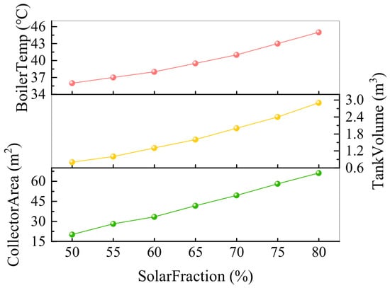
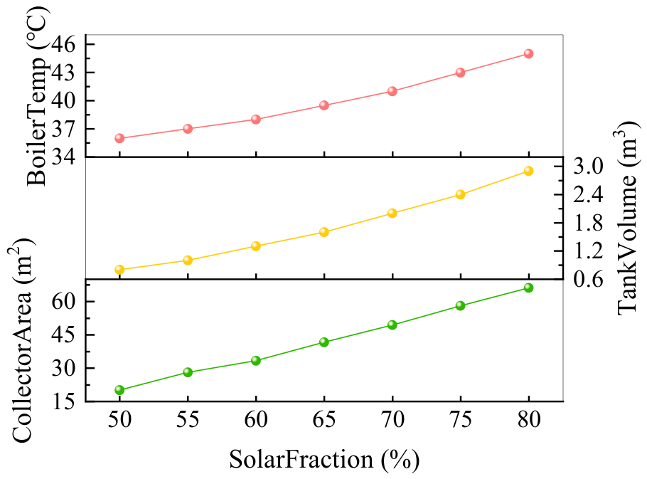
To clarify the influence of each decision variable on solar utilization performance, representative optimal solutions corresponding to different solar fractions were selected from the Pareto-optimal set. The variations in solar collector area, thermal storage tank volume, and biogas boiler start-up temperature were analyzed as the solar fraction increased from 50% to 80%. Figure 10 presents the variation trends of each optimization variable with respect to solar fraction. This analysis identifies the key factors affecting system performance and supports the selection of the final compromise solution.
Figure 10.
Influence of optimization variables on solar fraction.
Figure 10 shows that all three decision variables increase with solar fraction, although at different rates. The collector area exhibits the largest increase, from approximately 20 to 65 m2, confirming that greater solar collection capacity is the primary means of increasing solar heat supply and reducing biogas-boiler operation. The storage-tank volume increases from about 0.8 to 2.8 m3, enhancing solar-energy storage and mitigating fluctuations in solar radiation. Its more rapid increase above a solar fraction of 70% indicates the greater storage requirement of high-solar-fraction systems.
The optimal boiler start-up temperature increases within a narrower range, from 36 to 45 °C, in coordination with the enlarged collector area and storage capacity. Although raising this threshold alone would activate the boiler earlier, the greater solar input keeps the tank temperature above the threshold for longer periods, thereby reducing boiler operation in the optimized configurations. Thus, the start-up temperature mainly serves as an operational control parameter rather than a dominant determinant of solar fraction. Solutions with solar fractions of 50–80% are selected for further quantitative analysis.
5.6. Comparison Between Pre- and Post-Optimization Schemes
5.6.1. Solar Fraction Comparison at Different Initial Investment Levels
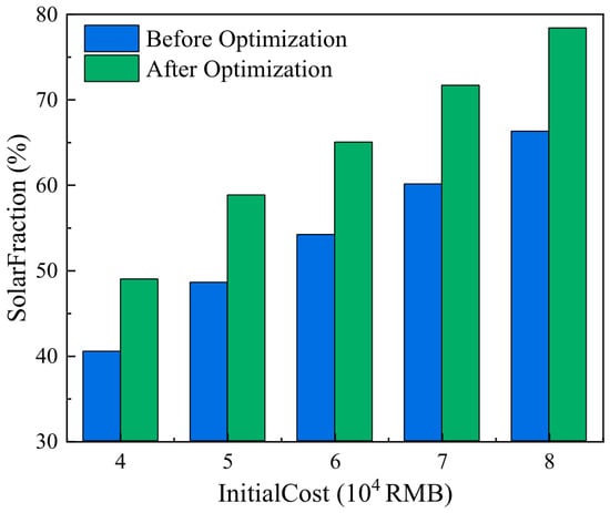
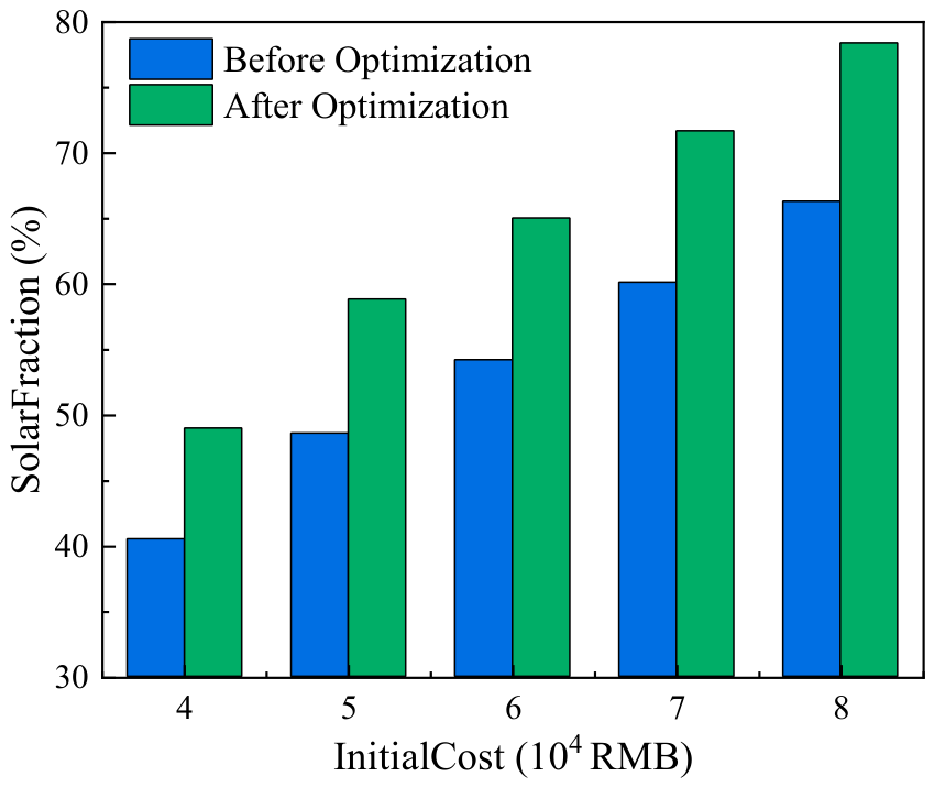
To evaluate the performance improvement achieved by the proposed optimization method, the solar fraction before and after optimization was compared under different initial investment levels. Based on the Pareto front, five representative investment levels—40,000, 50,000, 60,000, 70,000, and 80,000 CNY—were selected (Figure 11). For each investment level, the corresponding solar fractions before and after optimization were obtained, and the variation rates were calculated. This comparison further clarifies the contribution of the optimized design to renewable energy utilization.
Figure 11.
Comparison of solar fraction before and after optimization under different initial investment levels. (Note: All pre-optimization baseline configurations at varied costs are linearly scaled from a single conventional empirical design (); collector area and storage volume are scaled proportionally to match each target investment, with boiler start-up temperature fixed at 38 °C for all unoptimized cases.).
The pre-optimization solar fractions in Figure 11 were obtained from an author-defined reference configuration with . To generate budget-matched reference schemes, and were proportionally scaled and constrained within their prescribed bounds, while boiler start-up temperature was fixed at 38 °C. Each configuration was simulated using the same TRNSYS model. The reported 18–21% improvement in solar fraction is therefore conditional on this reference configuration and scaling method.
Figure 12 shows that, under all investment levels, the optimized solar fraction is consistently higher than that of the original design. This indicates that the proposed multi-objective optimization method effectively improves the system’s ability to utilize solar energy. As the initial investment increased from 40,000 CNY to 80,000 CNY, the solar fraction increased from 40.5% to 66.3% before optimization and from 48.98% to 78.40% after optimization. These results show that increasing system investment can improve both solar collection and thermal storage capacity, thereby increasing the share of solar energy in the total heating supply.
Figure 12.
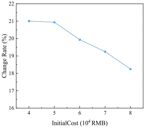
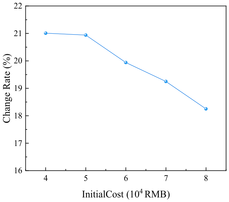
Relative improvement rates of solar fraction under different initial investment levels. (Note: The vertical axis “Change Rate (%)” denotes the relative growth rate of solar fraction, calculated as ; absolute gains are provided in percentage points (pp) for reference).
Figure 12 illustrates the improvement rate in solar fraction under different initial investment levels before and after optimization. The improvement rate remains within 18–21% across all investment levels, indicating that the proposed optimization method can enhance solar energy utilization under different system scales and that its performance is relatively stable.
Specifically, when the initial investment was 40,000 CNY, the improvement rate of solar fraction was 21.01%. As the investment increased to 50,000 CNY, the improvement rate decreased slightly to 20.94%. When the investment further increased to 60,000, 70,000, and 80,000 CNY, the improvement rates decreased to 19.94%, 19.25%, and 18.25%, respectively. This downward trend indicates a greater relative improvement in solar fraction at lower investment levels under the idealized assumption of unlimited biogas supply. However, the low-investment solutions also have lower solar fractions and substantially higher annual biogas demand. Their apparent optimization potential should therefore not be interpreted as superior practical feasibility when digester-heating consumption and finite winter biogas availability are considered. Through appropriate adjustment of key parameters, such as collector area, thermal storage tank volume, and boiler start-up temperature, solar utilization efficiency can be substantially improved. As the system investment increases, however, the configuration becomes more refined and the marginal benefit of further optimization decreases.
Although the improvement rate declines with investment, it remains above 18% at all investment levels, demonstrating that the optimization strategy consistently provides meaningful performance enhancement. For example, when the initial investment increased from 40,000 CNY to 80,000 CNY, the optimized solar fraction increased from 48.98% to 78.40%, representing substantial improvement relative to the pre-optimization results. This confirms that the proposed optimization model improves solar energy utilization and has good applicability and stability.
5.6.2. Comparison of Pre- and Post-Optimization Schemes Under the Compromise Solution
To further evaluate the performance improvement achieved by multi-objective optimization, the baseline design is compared with the quantitatively screened knee-point compromise solution on the Pareto front. Instead of subjective qualitative selection, the maximum curvature criterion is adopted to identify the reproducible optimal trade-off point on the Pareto curve.
The Pareto front describes the two conflicting objectives: maximizing SF and minimizing initial investment cost . For discrete Pareto solution points , the curvature of each point is calculated as [29]
where:
: curvature of the i-th discrete solution point on the Pareto front;
: normalized initial investment cost corresponding to the i-th Pareto solution;
: normalized solar fraction corresponding to the i-th Pareto solution;
: first-order difference approximate derivatives of and with respect to the serial number of adjacent Pareto discrete points;
: second-order difference approximate derivatives of and with respect to the serial number of adjacent Pareto discrete points.
Curvature calculation over all Pareto solutions yields the maximum curvature at SF = 69.7%, which falls within the 65–72% balanced performance interval and matches the previously proposed approximate 70% compromise scheme. This mathematically derived point is selected as the recommended optimized scheme for subsequent parameter and environmental benefit comparison. The key performance indicators of the initial scheme and the optimal compromise solution are compared in Table 8 to quantify the optimization effect.
Table 8.
Comparison of system performance before and after optimization.
Table 8 shows that all decision variables were adjusted after multi-objective optimization. The solar collector area increased from 40.0 m2 to 49.3 m2, corresponding to a 23.25% increase. This adjustment improves the system’s ability to capture solar radiation and allows more solar energy to be used for space heating, which is one of the main reasons for the increase in solar fraction. The thermal storage tank volume increased from 1.5 m3 to 2.0 m3, corresponding to a 33.33% increase. This indicates that the optimized system places greater emphasis on thermal energy storage and regulation, helping to mitigate solar radiation fluctuations and improve solar energy utilization efficiency.
The boiler start-up temperature increased from 38.0 °C to 41.0 °C, corresponding to a relatively small increase of 7.89%. If the tank-temperature profile remains unchanged, increasing the boiler start-up temperature causes the boiler to activate earlier rather than later. In the optimized compromise scheme, however, the increased start-up temperature is accompanied by a larger solar collector area and storage-tank volume. These capacity increases maintain the tank at a higher temperature and reduce the frequency and duration of boiler operation. Therefore, the reduced boiler operation results from the coordinated parameter configuration rather than from the higher start-up temperature alone. Compared with collector area and storage volume, the change in boiler start-up temperature is relatively limited, indicating that it mainly functions as an operational control parameter rather than a capacity-expansion parameter.
Regarding the optimization objectives, the solar fraction increased from 55.3% to 62.2%, corresponding to a relative improvement of 12.48% and an absolute gain of 6.9 percentage points. Meanwhile, the total initial investment increased from 54,750 CNY to 64,370 CNY, representing an increase of 9620 CNY, or 17.57%. These results indicate that the optimized configuration improves solar-energy utilization through the coordinated adjustment of the solar collector area, thermal storage-tank volume, and boiler start-up temperature, although this improvement requires additional initial investment.
In summary, an additional initial investment of 9620 CNY increased the solar fraction by 6.9 percentage points. The optimized scheme therefore provides improved solar-energy coverage while maintaining the initial investment within the examined design range. This result demonstrates the trade-off between upfront system cost and solar-energy utilization rather than indicating that the percentage improvement in solar fraction exceeds the percentage increase in investment.
To further reflect the long-term economic distinction of each scheme, the annual biogas consumption under each typical investment configuration is shown in Table 9, as higher initial investment with larger solar collector sizes reduces annual biogas combustion volume significantly.
Table 9.
Annual biogas consumption of representative optimized schemes.
Although the optimized annual biogas consumption decreases monotonically as the initial investment and solar fraction increase, the calculated CO2 reduction is not monotonic because it is evaluated relative to a different budget-matched baseline at each investment level. In particular, the biogas-consumption difference between the baseline and optimized schemes increases from 199 m3/a at 70,000 CNY to 245 m3/a at 80,000 CNY. Consequently, the avoided CO2 emission increases from 0.390 to 0.480 t CO2/a. This reversal reflects the changing difference between the paired baseline and optimized schemes rather than an increase in the absolute emissions of the optimized system.
The annual CO2 emission reduction generated by biogas savings is quantified via the following formula [30]:
where:
: annual CO2 reduction (t CO2/a);
: annual biogas consumption of the unoptimized baseline scheme under the same initial investment (m3);
: annual biogas consumption of the optimized scheme (m3);
: the regional average carbon emission factor for biogas combustion in Jiuquan.
The baseline biogas consumption values corresponding to the five investment levels are 1582, 1291, 1047, 836 and 661 m3, respectively, which are obtained from the linear-scaled traditional heating system, without multi-objective optimization.
As shown in Table 9, all optimized configurations deliver apparent carbon abatement benefits, with annual CO2 reduction ranging from 0.390 t to 0.504 t. The recommended compromise solution with a solar fraction of approximately 70% (initial investment of 70,000 CNY) achieves an annual carbon reduction of 0.390 t. These quantitative carbon-saving indicators echo the carbon-neutrality and low-carbon heating motivations illustrated in the Introduction, and further demonstrate the practical environmental value of the proposed solar–biogas optimization framework for rural buildings in Jiuquan.
5.6.3. First-Order Sensitivity to Digester-Heating Consumption
The TRNSYS model treats biogas as an unlimited ideal auxiliary source and does not include the parasitic energy required to maintain the anaerobic digester temperature. To estimate the order of magnitude of this effect, a first-order sensitivity analysis was conducted by assuming that digester heating consumes 30–60% of gross biogas production. If fdig is the fraction of gross production consumed by the digester, and Vbuilding is the building-side consumption reported in Table 9, the required gross production is calculated as
A 30% parasitic fraction therefore increases the required gross production by 42.9%, while a 60% fraction increases it by 150%. For the SF = 49.0% solution, gross production increases from 1325 m3/a of building-side consumption to approximately 1893–3313 m3/a. For the SF = 78.5% solution, the corresponding gross requirement is approximately 594–1040 m3/a. Thus, the practical effect is substantially greater at the low-solar-fraction end of the Pareto set.
Because the current optimization places no constraint on biogas availability and does not include biogas-production capacity or fuel cost in either objective, this first-order correction does not mathematically shift the calculated initial-investment–solar-fraction Pareto front. It instead increases the gross biogas-production requirement and may render some solutions infeasible when local winter production is limited. A quantitative displacement of the Pareto front would require a specified biogas-production constraint and a new TRNSYS–NSGA-II optimization.
6. Conclusions
In this study, a biogas-boiler-assisted solar heating system was established for a typical single-story rural residential building in Jiuquan, Hexi Corridor of Gansu Province. Mathematical models of the key components, including the solar collector, thermal storage tank, and biogas boiler, were established. Multi-objective optimization was performed using the NSGA-II algorithm, with the objectives of maximizing the solar fraction and minimizing the initial system investment. The main conclusions are as follows:
(1) Solar fraction generally increases with initial investment, while incremental performance improvement gradually weakens under the restriction of solar resources and heating load, showing typical diminishing marginal benefit. Detailed quantitative variation is shown in Section 5.5.
(2) The NSGA-II algorithm exhibits satisfactory convergence and uniform distribution of Pareto solutions, which can reliably resolve the dual-objective optimization of maximizing solar fraction and minimizing initial investment.
(3) Under the idealized assumption of unlimited biogas supply, relative to the author-defined reference configurations generated using the adopted proportional-scaling rule, the optimized solutions show an 18–21% increase in solar fraction over the examined investment range. The magnitude of this improvement is baseline-dependent and should not be generalized to other non-optimized system configurations. Low-investment solutions show greater relative improvement but also require substantially more biogas and are therefore more sensitive to digester-heating consumption and winter biogas availability.
(4) Within the present idealized model, the maximum-curvature criterion identifies a knee-point solution with a solar fraction of 69.7% (approximately 70%). This solution represents a compromise between initial investment and solar-energy utilization, but its practical deployment requires further verification under site-specific biogas-production and digester-heating constraints.
(5) Reasonable matching of collector area, heat storage capacity and boiler operation parameters is critical for improving the overall performance of the solar–biogas heating system, and this work provides theoretical guidance and parametric design references only for similar rural residential heating projects in Jiuquan, Hexi Corridor.
The results presented in this study represent a solar heating system assisted by an idealized biogas-fired boiler rather than a complete biogas-production and utilization chain. This study assumes an unlimited biogas supply and excludes digester-heating demand, seasonal production constraints, fuel costs, and operation and maintenance expenses. Consequently, the reported Pareto front represents the trade-off between initial investment and solar fraction rather than a complete lifecycle optimum. Future work should couple the heating model with a dynamic anaerobic-digestion model and include annualized lifecycle cost as an optimization objective.
Future work will establish a coupled anaerobic digestion thermal balance model to quantify seasonal biogas production and parasitic heat loss so as to eliminate the deviation caused by the ideal biogas boiler assumption.
Supplementary Materials
The following supporting information can be downloaded at: https://www.mdpi.com/article/10.3390/en19174162/s1.
Author Contributions
L.Y.: funding acquisition, conceptualization, writing—review and editing; S.Y.: writing—original draft and methodology; H.N.: writing—review and editing; Y.C.: writing—review and editing. All authors have read and agreed to the published version of the manuscript.
Funding
Fund Project: 2026 University Teachers’ Innovation Fund Project in Gansu Province: Research on the Application of Solar Building Integrated Heating System Based on Multi-Energy Complementary in Gansu Villages and Towns, Project No.: 2026A-232.
Data Availability Statement
The raw data supporting the conclusions of this article will be made available by the authors on request.
Conflicts of Interest
The authors declare no conflict of interest.
Glossary
| Nomenclature | |
| a | Performance coefficients |
| A | Area (m2) |
| C | ) |
| cp | Specific heat capacity, kJ/(kg·°C) |
| E | Load (kWh) |
| ) | |
| Heat removal factor of solar collector | |
| ) | |
| Hb | ) |
| m | Mass flow rate of the heat transfer fluid (kg/s) |
| P | Pareto solution set |
| IT | ) |
| Normalized initial investment of the i-th Pareto solution | |
| T | Temperature (°C) |
| V | Volume (m3) |
| Normalized solar fraction of the i-th Pareto solution | |
| Greek | |
| Efficiency | |
| Curvature at the i-th discrete Pareto point | |
| Density of heat transfer fluid (kg/m3) | |
| Temperature difference between fluid inlet and ambient (°C) | |
| Transmittance-absorptance product of collector | |
| Abbreviations | |
| EPS | Expanded Polystyrene |
| GA | Genetic Algorithm |
| IGD | Inverted Generational Distance |
| NSGA-II | Non-Dominated Sorting Genetic Algorithm II |
| PID | Proportional-Integral-Derivative controller |
| PSO | Particle Swarm Optimization |
| RE | Relative Error |
| SA | Simulated Annealing |
| SF | Solar Fraction |
| TMY | Typical Meteorological Year |
| TRNSYS | Transient System Simulation Tool |
| ZDT | Zitzler–Deb–Thiele test function |
References
- Fares, H.; Lobaccaro, G.; Gazbour, N.; Rasmussen, F.N.; Chèze, D.; Le Pierrès, N.; Wurtz, E. A Methodology for Assessing Environmental Impact of Building Integrated PV in Low Carbon Footprint Electricity Generation Context. Energy Build. 2025, 329, 115219. [Google Scholar] [CrossRef] [Scilit]
- Meister, C.; Schneeberger, S.; Jokiel, A.; Schuetz, P. Bottom-up Heat Pump Flexibility Estimation for Swiss Buildings Considering Monitored Building Data. Appl. Energy 2026, 414, 127856. [Google Scholar] [CrossRef] [Scilit]
- Ewart, M.; Santos, J.; Pacheco, A.; Monteiro, J.; Sequeira, C. On a New Method to Design Solar Photovoltaic Systems in Renewable Energy Communities: The Case of Culatra Island (Ria Formosa, Portugal). Energy 2023, 285, 129257. [Google Scholar] [CrossRef] [Scilit]
- Joshi, P.; Rao, A.B.; Banerjee, R. Review of Solar PV Deployment Trends, Policy Instruments, and Growth Projections in China, the United States, and India. Renew. Sustain. Energy Rev. 2025, 213, 115436–115453. [Google Scholar] [CrossRef] [Scilit]
- Barone, G.; Buonomano, A.; Kalogirou, S.; Ktistis, P.; Palombo, A. A Holistic Methodology for Designing Novel Flat Plate Evacuated Solar Thermal Collectors: Modelling and Experimental Assessment. Renew. Energy 2024, 232, 120967. [Google Scholar] [CrossRef] [Scilit]
- Al-Sharafi, A.; Ahmadullah, A.B.; Al-Buraiki, A.S. Influence of Dust Accumulation on the Performance and Economics of a Flat Plate Solar Collector System. Sol. Energy 2025, 300, 113879. [Google Scholar] [CrossRef] [Scilit]
- Mausam, K.; Singh, S.; Ghosh, S.K.; Singh, R.P. Thermal Performance Modelling of Solar Flat Plate Parallel Tube Collector Using ANN. Energy 2024, 303, 131940. [Google Scholar] [CrossRef] [Scilit]
- Wang, D.; Mo, Z.; Liu, Y.; Ren, Y.; Fan, J. Thermal Performance Analysis of Large-Scale Flat Plate Solar Collectors and Regional Applicability in China. Energy 2022, 238, 121931. [Google Scholar] [CrossRef] [Scilit]
- Bhadra, S.; Mwesigye, A. Influence of Control Strategy on the Energetic Performance of an Air Source Heat Pump Coupled with a Solar Air Collector for Domestic Hot Water in a Cold Climate. Renew. Energy 2025, 244, 122682–122699. [Google Scholar] [CrossRef] [Scilit]
- Chen, M.; Wei, J.; Yang, X.; Fu, Q.; Wang, Q.; Qiao, S. Multi-Objective Optimization of Multi-Energy Complementary Systems Integrated Biomass-Solar-Wind Energy Utilization in Rural Areas. Energy Convers. Manag. 2025, 323, 119241. [Google Scholar] [CrossRef] [Scilit]
- You, J.; Gao, J.; Li, R.; Wang, R.; Xu, Z. Air-Source Heat Pump Assisted Absorption Heat Storage for Discharging under Low Ambient Temperature. Appl. Energy 2025, 380, 125121. [Google Scholar] [CrossRef] [Scilit]
- Sadeghi, A.; Maleki, A.; Haghighat, S. Techno-Economic Analysis and Optimization of a Hybrid Solar-Wind-Biomass-Battery Framework for the Electrification of a Remote Area: A Case Study. Energy Convers. Manag. X 2024, 24, 100732. [Google Scholar] [CrossRef] [Scilit]
- Li, F.; Tian, H.; Shen, H.; Zhang, X.; Liu, J.; Gong, Z. A Preference Modified Inverted Generational Distance Indicator Guided Algorithm for Evolutionary Multi-Objective Optimization. Swarm Evol. Comput. 2025, 99, 102169. [Google Scholar] [CrossRef] [Scilit]
- Han, Z.; Han, W.; Ye, Y.; Sui, J. Multi-Objective Sustainability Optimization of a Solar-Based Integrated Energy System. Renew. Sustain. Energy Rev. 2024, 202, 114679. [Google Scholar] [CrossRef] [Scilit]
- Li, Y.; Hu, W.; Zhang, F.; Li, Y. Multi-Objective Collaborative Operation Optimization of Park-Level Integrated Energy System Clusters Considering Green Power Forecasting and Trading. Energy 2025, 319, 135055. [Google Scholar] [CrossRef] [Scilit]
- Ahmad, A.; Yadav, A.K.; Ali, S.; Mazid, A.; Gautam, R.K.S.; Yadav, A. A Hybrid Machine Learning-NSGA-II-TOPSIS Framework for Multi-Objective Optimization of CI Engine Performance and Emissions Using Ternary Biodiesel-Butanol-Diesel Blends. Case Stud. Therm. Eng. 2026, 82, 108047. [Google Scholar] [CrossRef] [Scilit]
- De, S. A Hybrid Neighbourhood-Based Fuzzy NSGA-II–MOPSO Algorithm for Solving Multi-Objective Optimization Problems under Uncertainty. Appl. Soft Comput. 2026, 199, 115233. [Google Scholar] [CrossRef] [Scilit]
- Liu, Z.; Gao, X.; Huang, X.; Xie, Y.; Gao, J.; Yang, X.; He, Q. Evaluation on Solar-Biogas Heating System for Buildings: Thermal Characteristics and Role of Heat Storage Sectors. Appl. Energy 2025, 390, 125817. [Google Scholar] [CrossRef] [Scilit]
- Sun, T.; Chong, W.T.; Mohd Khairuddin, A.S.; Tey, K.S.; Wei, Y.; Han, D.; Wu, J.; Pan, S. Bi-Objective Optimization of a Solar-Assisted Biogas and Air-Source Heat Pump System for Rural Heating Applications. Appl. Therm. Eng. 2025, 280, 128164. [Google Scholar] [CrossRef] [Scilit]
- Xiao, Y.; Yang, L.; Wang, X.; Yu, Y. Adaptability Design of Solar Heating Systems in Rural Residences and Model Predictive Control-Based Differentiated Indoor Temperature Control: A Case Study in Northern Shaanxi. Appl. Therm. Eng. 2026, 292, 130246. [Google Scholar] [CrossRef] [Scilit]
- Cao, Y.; Chen, Y.; Ren, P.; Wang, D.; Zhuang, Z.; Zhou, W. Modeling and Performance Analysis of Solar Energy and Biogas Complementary Heating System in Rural Areas. Appl. Therm. Eng. 2025, 271, 126283. [Google Scholar] [CrossRef] [Scilit]
- Zhang, L.; Hou, Y.; Liu, Z.; Du, J.; Xu, L.; Zhang, G.; Shi, L. Trombe Wall for a Residential Building in Sichuan-Tibet Alpine Valley—A Case Study. Renew. Energy 2020, 156, 31–46. [Google Scholar] [CrossRef] [Scilit]
- GB/T 50824-2013; Design Standard for Energy Efficiency of Rural Residential Buildings. China Architecture & Building Press: Beijing, China, 2013.
- Shang, L.; Gao, B.; Yang, D.; Li, S.; Yu, H. Design Research on Improving the Environmental Performance of Rural Dwellings in China’s Hexi Corridor with Seasonal Room Rotation. Buildings 2025, 15, 4263. [Google Scholar] [CrossRef] [Scilit]
- Li, A.; Gao, X.; Yang, L. Field Measurements, Assessments and Improvement of Kang: Case Study in Rural Northwest China. Energy Build. 2016, 111, 497–506. [Google Scholar] [CrossRef] [Scilit]
- Pal, A.; Ilango, G.S. Design and Techno-Economic Analysis of an off-Grid Integrated PV-Biogas System with a Constant Temperature Digester for a Cost-Effective Rural Application. Energy 2024, 287, 129671. [Google Scholar] [CrossRef] [Scilit]
- Hao, J.; Yang, X.; Wang, C.; Tu, R.; Zhang, T. An Improved NSGA-II Algorithm Based on Adaptive Weighting and Searching Strategy. Appl. Sci. 2022, 12, 11573. [Google Scholar] [CrossRef] [Scilit]
- Wang, X.; Wang, X.; Qin, B. Improved Multi-Objective Differential Evolution Algorithm and Its Application in the Capacity Configuration of Urban Rail Photovoltaic Hybrid Energy Storage Systems. J. Energy Storage 2024, 98, 113155. [Google Scholar] [CrossRef] [Scilit]
- Kong, X.; Zhi, J.; Shan, T.; Gao, J.; Wang, Z.; Yang, S. Multi-Objective Optimization and Energy Absorption Mechanisms of Bio-Inspired Lightweight Sandwich Structures Based on Pareto Representative Solutions. Compos. Struct. 2026, 394, 120674. [Google Scholar] [CrossRef] [Scilit]
- Liu, X.; Wang, Z.; Wang, J.; Xing, L.; Li, J.; Dong, Z.; Li, M.; Han, Y.; Cao, J. Characteristics of PM2.5 Bounded Carbonaceous Aerosols, Carbon Dioxide and Its Stable Carbon Isotopes (δ13C) in Rural Households in Northwest China: Effect of Different Fuel Combustion. J. Environ. Manag. 2024, 359, 121004. [Google Scholar] [CrossRef] [Scilit] [PubMed]

Disclaimer/Publisher’s Note: The statements, opinions and data contained in all publications are solely those of the individual author(s) and contributor(s) and not of MDPI and/or the editor(s). MDPI and/or the editor(s) disclaim responsibility for any injury to people or property resulting from any ideas, methods, instructions or products referred to in the content. |
© 2026 by the authors. Licensee MDPI, Basel, Switzerland. This article is an open access article distributed under the terms and conditions of the Creative Commons Attribution (CC BY) license.