


Abstract
The intermittent nature of solar energy requires precise capacity and battery sizing for reliable microgrid design. Extending beyond traditional annual photovoltaic maps, we introduce a methodology for high-resolution capacity sizing surfaces that integrate hourly solar irradiance and battery storage estimation from averaged meteorological data, demonstrated here for Winnipeg, Canada. Leveraging pvlib Python 3.13 library, we simulate performance across all module orientations using photovoltaic modules with 22.5% efficiency and lithium-ion batteries assuming 92% round-trip efficiency, defining core metrics—Capacity ratio, Storage ratio, Excess ratio, and Battery cycling ratio, including Battery charging and discharging C-rates—while incorporating system losses. The analysis further embeds hourly unmet load and average battery state of charge. Unlike conventional PV-yield tools and single-configuration microgrid studies, the present method combines site-specific hourly meteorological data, full tilt–azimuth evaluation, battery dispatch, and explicit compliance-linked PV and storage sizing. These intuitive capacity sizing surfaces reveal how hourly modeling resolves diurnal and seasonal structure that monthly-average tools omit; a sensitivity analysis bounds the residual effect of inter-annual variability removed by climatological averaging, enhancing reliability and battery longevity under variable target standard deviation of compliance ranging from to . Open-access capacity sizing surfaces for Canada-wide at 564 stations and an open-source Python library that reproduces the methodology for any hourly meteorological dataset world-wide are provided to easily size solar PV and battery systems.
1. Introduction
The global transition toward sustainable energy requires rapid and effective integration of renewable technologies. By converting abundant sunlight into electricity, solar photovoltaic (PV) systems offer a scalable path to increasing renewable energy share of any country, directly supporting global net-zero emissions targets [1,2]. This is particularly relevant in Canada, which has committed to achieving a net-zero electricity grid [3]. As of 2024, Canada has over 5 GW of installed solar PV capacity, and the solar sector has expanded nearly 92% over the past five years [4]. However, the inherent intermittency of solar resources challenges grid reliability, making the co-deployment with battery energy storage systems (BESSs) essential for off-grid applications and for maximizing self-consumption in grid-tied systems [1,5].
Sizing of PV arrays and batteries for grid and off-grid applications is fundamental to the technical and economic viability of solar-plus-storage systems [6,7,8,9]. Undersized systems risk power deficits, while oversized configurations inflate costs and waste resources [10,11,12,13]. This challenge is amplified in the built environment, where real-world installation constraints often preclude optimal conditions. Architects and engineers often design systems with sub-optimal orientations—such as east- or west-facing facades for building-integrated photovoltaic (BIPV) or low-tilt angles on flat roofs—instead of the south-facing, latitude-optimal tilt that maximizes annual yield [14,15]. Since the magnitude and temporal profile of energy generation are highly sensitive to tilt and azimuth, optimal system sizing must account for this full spectrum of possible configurations [12,16,17].
In Canada, stakeholders have traditionally relied on Photovoltaic Potential Maps developed by Natural Resources Canada (NRCan) [18,19] as shown in Figure 1, which provide average daily and annual PV energy potential on a grid at approximately 2 km spatial resolution, typically assuming optimal tilt and south-facing orientations without accounting for storage requirements [19]. Complementary tools such as RETScreen [20,21,22] and HOMER [23] have been widely adopted for techno-economic evaluation, but both rely on monthly averaged data or TMY datasets that lack the temporal fidelity required for accurate battery sizing [22,24].
Figure 1.
Geographic photovoltaic-resource maps for Canada from NRCan (© Her Majesty the Queen in Right of Canada, as represented by the Minister of Natural Resources, 2020) [18] and EnergyHub [25]. These maps show solar-resource or PV-yield potential at geographic locations and are included for context only; they do not provide battery-storage requirements or orientation-specific capacity-sizing results.
To improve temporal granularity, global and national datasets such as NASA POWER, Global Renewables Watch, and Environment and Climate Change Canada’s CWEEDS, and Canadian Weather Year for Energy Calculations (CWEC) provide hourly irradiance and meteorological data for over 560 stations across Canada [26,27]. These datasets capture hourly fluctuations in global, direct, and diffuse irradiance—essential for assessing diurnal variability and its implications for PV and battery performance. However, such data are seldom visualized or synthesized into practical sizing tools that correlate orientation with PV and battery performance outcomes.
Recent research on PV-BESS optimization has employed advanced computational techniques but often focuses on idealized conditions or single sites [12]. For example, Chang et al. [28] optimized PV and battery sizes using hourly data but considered only a limited range of tilt angles, assuming fixed azimuth orientation. Such simplifications limit the generalizability of findings across Canada’s diverse climates and installation contexts. Furthermore, most optimization studies emphasize energy yield or reliability while neglecting long-term battery cycling and degradation, which significantly influence lifecycle costs and sustainability.
While existing tools and studies provide valuable insights, they exhibit critical limitations [22]. Therefore, this paper introduces a comprehensive framework for generating high-resolution solar capacity sizing mapping surfaces (CSSs) for solar PV and battery storage systems in Canada. The framework leverages high-fidelity, hourly meteorological data and simulates performance across the full spectrum of tilt and azimuth combinations. This work presents an open-source methodology for generating solar-plus-storage capacity-sizing surfaces from hourly station data. Unlike PV-yield tools that report generation potential alone and single-configuration microgrid studies that optimize a limited set of candidate designs, the method evaluates the full tilt–azimuth design space and couples each orientation to battery dispatch at a user-selected compliance level. The resulting outputs include production (P) capacity ratio (), storage ratio (), excess ratio (), battery cycling ratio (), charge and discharge C-rate indicators ( and ), state of charge (), and hourly unmet load (). Together, these metrics allow designers to compare PV capacity, usable storage, curtailment, battery cycling-related stress, and temporal supply deficits within one consistent framework.
Contributions
This paper introduces several novel contributions that distinguish it from existing tools and methodologies:
- 1.
- Comprehensive capacity sizing surfaces: Unlike existing PV potential maps (NRCan, EnergyHub) that provide only average annual yield for optimal orientations, our surfaces provide , , , , and C-rates across the full spectrum of tilts—0–90°—and azimuths—0–360°. This enables system designers to quantify the trade-offs between sub-optimal orientations—e.g., building-integrated PV—and the required PV and battery capacity.
- 2.
- Integration of battery storage sizing with reliability targets: While tools like RETScreen and HOMER can perform battery sizing, they do not provide spatially explicit, pre-computed mapping of storage requirements. Our methodology generates surfaces at six compliance levels ( to ), directly linking reliability targets to storage capacity.
- 3.
- Battery stress metrics: We introduce novel metrics— (cumulative energy throughput), (charging C-rate), and (discharging C-rate)—that quantify battery operational stress and provide early indicators of degradation. These metrics are absent from existing PV tools.
- 4.
- -scaling framework: The use of statistical sigma levels as compliance targets provides an intuitive, continuous scale for reliability specification, bridging the gap between engineering metrics and practical design requirements.
- 5.
- Open-access dataset and library: The pre-computed dataset for Canada—564 stations, NBR analysis—and the accompanying Python library abstract away the complexity of low-level pvlib simulations, providing a condensed parametric space that reduces computational cost for downstream optimization and search procedures.
2. Literature Review
2.1. Solar PV Technology for Sustainable Energy and Building Integration
The need for global action to mitigate climate change has driven increased interest in solar energy, which is essential for protecting Earth’s biodiversity [29]. Kumar and Rathore [30] found that solar energy has minimal environmental impact, underscoring its importance in renewable energy modeling across diverse climates. Recent advancements in solar PV technology have significantly accelerated its adoption due to declining costs and improved efficiency [31]. The global solar PV market has witnessed substantial growth, with cumulative installed capacity surpassing by the end of 2025, driven by government incentives and technological innovations. Applications range from off-grid systems serving remote areas to building-integrated solutions, highlighting the versatility and environmental benefits of solar energy.
Solar PV modules can be categorized as either monofacial or bifacial. Previous studies have shown that bifacial PV systems, which capture solar energy from both sides, can generate 5% to 30% more power compared to conventional monofacial modules, depending on factors such as albedo and installation geometry [32,33,34,35]. To further increase energy yield, tracking mechanisms are often employed. Studies indicate that single-axis trackers can improve annual energy production by 16% to 25%, while dual-axis trackers can achieve increases of 25% to 40% compared to fixed-tilt systems [36,37]. Recent work has demonstrated that combining bifacial modules with dual-axis tracking provides synergistic benefits that significantly enhance performance [38].
2.2. BESS for Solar PV Integration
The integration of BESS with solar PV has gained significant attention as a means to enhance energy reliability and mitigate intermittency of solar power [39]. These systems enhance power quality and grid reliability in hybrid renewable configurations [40]. Recent studies have focused on optimizing battery storage to maximize efficiency and operational performance [41,42]. Mathematical modeling and controlled cell-level tests indicate that charge and discharge efficiencies of lithium-ion batteries can exceed 99% under ideal, low-C-rate conditions [43], while round-trip efficiencies typically range from 90% to 98% when internal resistance and state-of-charge effects are minimized [41,44]. In real-world system operation, however, round-trip efficiencies are frequently lower—sometimes dropping by as much as 33%—due to higher C-rates, temperature variations, inverter losses, and auxiliary power consumption. Zhou et al. [45] observed that residential BESS units rarely discharge at more than 25% to 40% of rated power during peak-demand events, resulting in higher-than-expected grid imports and reduced economic benefits. These findings indicate that technological improvements alone are insufficient; continuous optimization of sizing, control strategies, and operational dispatch remains essential for maximizing the value of solar-plus-storage systems [45,46,47].
Optimization is especially important in off-grid and hybrid systems, where techno-economic analyses show that properly sizing PV-BESS systems is crucial for achieving both cost-effectiveness and energy security [5,47,48]. Flexibly using stored energy enhances system resilience and ensures that energy supply closely matches demand. Moreover, regulatory frameworks and utility rate structures strongly influence the adoption of solar and storage systems, as they can either incentivize or discourage investment [49].
Integration with complementary technologies such as vehicle-to-grid (V2G) and demand-side management offers additional operational flexibility [50,51,52,53], but the present study focuses on the sizing of PV and stationary storage for a fixed load; such extensions are identified as future work.
2.3. Solar PV Modeling Techniques and Software Tools
Accurate modeling of solar PV systems is required for optimizing design, forecasting energy yield, and assessing economic viability across diverse climatic conditions and configurations. Common modeling techniques include empirical models, such as the single-diode equivalent circuit for module-level simulation, transposition models like Perez [54] or Hay–Davies [55] for calculating plane-of-array irradiance, and temperature correction models using parameters like Nominal Operating Cell Temperature or the Sandia Array Performance Model [56]. These principles are implemented in a variety of software tools, each suited to different levels of detail and application scales.
For preliminary feasibility studies, PVWatts is a widely used tool because it requires minimal input data while providing reasonable accuracy. Validation studies have demonstrated its general accuracy within ±10% for most locations. Significant improvements were made in Version 5, which addressed a systematic underprediction issue in earlier releases; the updated version produces annual AC energy estimates within 1.8% of measured values, a major enhancement from the previous 11.9% underprediction [57]. Improvements have been made to the NREL PVWatts model to enhance the accuracy of energy output predictions for fixed and one-axis tracking photovoltaic systems by incorporating detailed loss calculations and bifacial gain estimation [58]. While ideal for initial screening, PVWatts simplifies complex phenomena like shading and spectral effects, making it less suited for highly detailed engineering analyses [57].
For more comprehensive techno-economic modeling, specialized software packages such as HOMER, RETScreen, and the system advisor model (SAM) are employed [21,23,59,60]. HOMER specializes in optimizing hybrid microgrids by simulating various configurations of solar PV, wind, diesel generators, and storage systems to minimize cost [61]. SAM provides detailed, hour-by-hour simulations of grid-connected systems with extensive customization options for utility-scale applications [21,62,63]. RETScreen, an Excel-based platform, excels in feasibility and life-cycle assessments and has been validated to predict energy yields within 1–2% of measured data for grid-connected PV [64,65].
In recent years, the open-source Python library pvlib has emerged as a flexible, research-oriented modeling platform. Originally developed by Sandia National Laboratories, pvlib incorporates peer-reviewed algorithms for the entire PV simulation chain—from solar position and clear-sky irradiance to DC/AC power conversion [66,67,68]. Its modular, object-oriented structure enables high transparency and customization. Researchers can integrate pvlib with time-series weather data and advanced modules to account for spectral effects, soiling losses, and bifacial performance. Validation studies have shown that pvlib achieves a root mean square error below 5% in utility-scale PV performance forecasting [67].
While established tools and maps provide a critical foundation for solar energy adoption, they have significant limitations for precise microgrid and solar-plus-storage design. Tools like RETScreen and national PV maps typically rely on monthly averaged data, which lacks the hourly resolution needed to accurately capture the dynamic interplay between solar generation, battery operation, and load demand. Moreover, they offer little or no integration of energy storage sizing and provide no specific metrics linking battery capacity to target compliance levels. A related persistent challenge in the literature is determining the installed PV capacity in required to deliver, on average, 1 of usable power throughout the year—accounting for orientation, location-specific weather patterns, and system losses—particularly when paired with storage. Existing studies and tools rarely provide this information in a pre-computed, spatially explicit form. Unlike RETScreen and PVWatts, which rely on monthly or annual averaged irradiance and do not size storage, and unlike HOMER, which for many Canadian sites falls back on TMY or global datasets when local hourly measurements are unavailable, the present method combines site-specific hourly irradiance with battery-dispatch simulation across the full tilt–azimuth space, and ties both array and storage size directly to a user-selected compliance level. To address this gap, this study introduces the first high-resolution CSS for Canada. These maps integrate hourly meteorological data with battery storage simulation across all possible PV tilt and azimuth orientations, while introducing novel performance and lifetime metrics to guide both PV and storage sizing decisions. The approach is also focused on simplifying training data to develop AI agents.
3. Methodology
This section describes the systematic approach for creating CSS for solar PV systems with battery storage. The methodology uses site-specific, hourly meteorological data from the Winnipeg International Airport. The process leverages the open-source Python library pvlib for PV performance modeling and a custom algorithm to simulate energy flows. All calculations are conducted on an hourly basis over a full year (8760 timesteps) to capture diurnal and seasonal variations, ensuring high-fidelity results suitable for AI training datasets and practical system design. To ensure reproducibility, all input data are sourced from publicly available CWEEDS provided by NRCan. The methodology can then be applied to any meteorological data worldwide.
3.1. Data Acquisition and Preprocessing
Hourly meteorological data was obtained from the NRCan CWEEDS archive, which contains data for 564 locations [26]. This study uses data specifically from the Winnipeg International Airport station.
Generating capacity sizing maps requires solar irradiance data, including global horizontal irradiance, diffuse horizontal irradiance, and direct normal irradiance. Additional parameters, such as dry-bulb temperature and wind speed, are also incorporated into the pvlib model to improve simulation accuracy. The raw CWEEDS data required unit conversion, as irradiance was provided in and wind speed was stored in tenths of a metre per second ( ). In-house scripts were developed to convert these values to and , respectively, and to format the refined dataset into optimized DataFrames.
A continuous hourly timeline was generated using pandas.date_range, spanning the full period of the CWEEDS data while ignoring leap days. Local time zones required by pvlib, were automatically assigned from station coordinates using the TimeZoneFinder library.
Rather than constructing a formal typical meteorological year (TMY) using the Sandia month-selection method [69], a climatological average meteorological year was computed by taking the multi-decadal hourly mean of each weather variable for all 8760 h of the year. This climatological averaging approach has two important implications. First, it removes inter-annual variability and extreme weather events, making the results more representative of long-term average performance rather than worst-case scenarios. This is intentional, as the aim is to provide a consistent baseline for system sizing across locations. Second, the approach does not capture multi-day cloudy periods that are critical for battery sizing, particularly at higher compliance levels— and . While this represents a limitation for guaranteeing reliability in specific years, it provides a conservative and standardized approach for planning-level designs. The sensitivity of the results to the choice of weather year is quantified in the results discussion. For more rigorous reliability assessment, practitioners can use the provided methodology to run individual years—including the worst in the historical record—to assess variability. This method removes inter-annual variability and extreme events, is particularly well-suited for generating nationwide parametric sizing plots that represent long-term average performance rather than year-to-year fluctuations or worst-case conditions. Missing data were linearly interpolated prior to averaging.
The processed dataset is stored to avoid repeating the preprocessing step and to facilitate its use in downstream design exploitation and data-driven applications [70,71].
3.1.1. Bifacial Irradiance Modeling
Rear-side irradiance was computed by transposing the diffuse and ground-reflected components onto the module back surface, defined by the front-surface tilt and azimuth rotated by 180°, and scaling the resulting rear plane-of-array irradiance by a bifaciality factor of 0.85. Ground-reflected irradiance uses an isotropic reflection assumption with an albedo of 0.25, specified in the model input file. The implementation was additionally benchmarked against PVWatts in Agyei-Agyemang et al. [71], using the same hourly meteorological inputs and comparable PV configuration assumptions. This cross-model comparison provides an implementation check for the simulated PV output; however, it does not constitute experimental validation of rear-side irradiance, snow-albedo effects, or installation-geometry effects. The bifacial calculations use a two-surface irradiance approximation with a fixed albedo and bifaciality factor. Row spacing, clearance height, ground-coverage ratio, view factors, mutual shading, rear-side irradiance non-uniformity, and seasonally varying snow albedo are not represented. Therefore, the bifacial outputs, particularly for vertically mounted configurations, should be interpreted as comparative results under the stated assumptions rather than experimentally validated, site-specific bifacial-yield predictions. Future work should apply a geometry-resolved bifacial model with site-specific installation parameters and seasonal ground-reflectance inputs.
3.1.2. PV Conversion, Temperature, and Loss Models
Hourly AC PV output was simulated in pvlib using in-house module and inverter parameter sets developed from manufacturer specifications. The module parameter was formatted to match the parameters in the Sandia database, while the inverter parameter set followed the CEC inverter-model parameter structure required by pvlib. Cell temperature was calculated using the Sandia array performance model (SAPM) temperature model based on hourly plane-of-array irradiance, ambient temperature, and wind speed.
The model included physical angle-of-incidence effects and inverter conversion, while spectral losses were not modelled. For bifacial configurations, front- and rear-side irradiance were evaluated separately, converted to AC output independently, and then summed. The reported PV output therefore reflects irradiance, cell-temperature, angle-of-incidence, and inverter-conversion effects without imposing a separate aggregate PV loss factor.
3.2. Compliance Levels and -Scaling
The performance of the solar-battery system is evaluated against a set of compliance targets expressed in standard deviations, . This -scale provides a continuous, intuitive way to specify how the system must meet the load, ranging from basic to critical performance levels. Each level corresponds to a target percentage of the total load that the system is designed to satisfy, analogous to statistical confidence intervals. For instance, corresponds to 68.27% compliance, meaning the system is designed to supply 68.27% of the total expected load over the analyzed period.
It is important to clarify that using as a compliance scale does not assume the unmet load follows a normal distribution. Rather, the normal distribution is referenced as a widely recognized statistical framework to define discrete, ascending compliance tiers. This approach provides a standardized metric that correlates directly with traditional engineering reliability metrics such as loss of load probability (LOLP), while offering a more intuitive scaling for design specification.
3.3. Definition of Parameters
3.3.1. Solar Production for 1
System sizing begins by determining the energy output of a solar peak capacity of 1 PV system at standard test conditions (STCs). The P metric represents the total AC electrical power generated by this 1 system over the simulation period, expressed in . P is calculated by running an hourly simulation in pvlib that accounts for local irradiance, angle-of-incidence effects, module-temperature effects, and inverter conversion. The total P for any period is the sum of these hourly power values. This metric quantifies the actual site- and orientation-specific energy resource available from 1 of installed PV capacity and serves as the foundational reference for all subsequent sizing calculations. All calculations are conducted for actual temperatures compared to STC.
3.3.2. Capacity Ratio
This is a dimensionless oversizing factor used to determine the required solar peak capacity to meet a scalable unit load. The calculation is based on a per-unit reference load of 1 denoted as 1 , where the subscript ‘u’ indicates this scalable unity basis. The reference load is held constant at 1 across all 8760 h. This normalization makes the results scalable to any load magnitude by simple multiplication, but it removes any diurnal or seasonal demand structure; consequently, configurations cannot be evaluated here for their alignment with a realistic time-varying load profile, and this is stated as a limitation of the present study. The open-source implementation supports arbitrary load profiles, enabling future extensions to time-varying demand.
The accounts for solar intermittency, resource variability, and system losses from factors like shading, soiling, DC-AC conversion, temperature, and degradation. Since solar power is intermittent, more are needed to match a steady 1 output. For example, to replicate the annual output of a 1 generator running constantly, the solar array must be oversized to generate surplus energy during peak sunlight hours, compensating for downtime and inefficiencies. Here, denotes the peak power capacity of the solar module (STC: 1000 irradiance, 25 °C cell temperature), which is the industry-standard maximum output rating. In contrast, the ideal energy output assumes the panel runs continuously at its nameplate rating—say, 700 —for every hour of the analysis period.
represents the deficiency arising from the solar resource falling short of the standard peak irradiance of 1000 and all energy losses incurred during battery charging and discharging, and other system processes. A of 5, for example, means 5 of any combination of solar modules are required for every 1 of solar production. provides the essential first step in system design—determining the total size of the solar array required. A high means that we have a low capacity factor of the solar resource and high energy losses that have to be recreated.
The methodology for calculating incorporates the PV-conversion effects represented in the hourly model and battery charging/discharging inefficiencies. Since PV capacity and storage requirements interact dynamically, is solved iteratively alongside until convergence. Computations are performed in Python using pvlib for PV modeling and a custom module called CSMlib to complete calculations.
3.3.3. Storage Ratio
The determines the battery capacity required to produce more steady and reliable power when solar production is unavailable. is defined by
where B is the battery capacity in required to meet a unit target load, . An of 4 means 4 of battery storage is needed per 1 of target output. determines the size of the energy storage system needed to achieve a desired compliance level. Solar power stops at night and is affected during cloudy weather. For a given compliance level, defines the minimum storage required to address the intermittency of solar to the target level.
The methodology for sizing the battery to meet a compliance target involves analyzing its performance over a selected period, typically a month or a full year. To calculate , we measure the energy deficit ratio, which is the ratio of the unmet energy load to the total expected load.
For example, to meet a (68.27% reliability) compliance level, the system’s energy shortfall must not exceed 31.7% of the time, resulting in a target fraction of 0.317. The analysis assumes a battery with a 100% depth of discharge (DOD) with an initial of 0.5. The 100% DOD was adopted to establish a conservative, chemistry-independent lower bound on the usable battery energy required to meet each compliance target; , as reported, therefore denotes usable, not nameplate, capacity. In practice, lithium-ion BESS installations restrict usable DOD to approximately 80–90% to limit deep-discharge degradation, although some commercial systems permit wider operating windows, so the nameplate capacity required in practice is correspondingly larger: . A configuration reported here at = 4 / therefore corresponds to approximately = 5 / of installed nameplate capacity at an 80% DOD limit. Practitioners should apply this scaling when translating into a procurement specification, and the degradation-related discussion in the results should be read as pertaining to usable-energy cycling under this convention. The charging and discharging efficiencies are set at 0.96, aligning with previous study reports [41,43]. Once is determined, it feeds into the iterative calculation of for convergence, ensuring the solar array and storage are co-optimized.
3.3.4. Excess Ratio
The quantifies the energy that is produced but could not be stored. This situation occurs when solar panels are producing power, but the battery is fully charged and the immediate electrical load of 1 is satisfied. In grid-connected applications, this surplus energy can be exported to the grid. In off-grid systems, the power electronics typically curtail the solar production, or excess energy may be diverted to a secondary use, such as heating water.
A high indicates that a significant amount of energy is being clipped or curtailed. This can represent an opportunity to utilize that energy, for instance by selling it to the grid, shifting flexible loads, or increasing the battery storage capacity if it is cost-effective. The is highly dependent on the compliance level selected.
3.3.5. Battery Cycling Ratio
A new metric that measures the cumulative battery cycling, called the battery cycling ratio, , is the cumulative energy in that was used to charge and discharge the battery over the time period. It represents the magnitude of flow of energy in and out of the battery. It is non-dimensionalized by dividing the cumulative energy by the battery capacity and thereby has units of . is a direct indicator of battery usage and stress. A higher value signifies more frequent cycling, which accelerates degradation and has direct implications for the battery’s lifespan. This metric helps in selecting battery chemistry with a suitable cycle life and forecasting long-term maintenance costs directly from the new solar resource maps being developed with the proposed methodology.
3.3.6. Battery Charging and Discharging C-Rates
The battery charging C-rate, , and discharging C-rate, , metrics quantify the average rate at which energy is moved into and out of the battery during a specified period.
They are defined as the ratio of the average charging or discharging power to the corresponding battery capacity. The units are in or C. While reveals the total amount of energy cycled, the C-rates describe the intensity of that cycling. High C-rates contribute significantly to battery stress and degradation. Together, these metrics provide a comprehensive view of both the cumulative usage, and the operational intensity, and , to assess the impact on battery lifespan.
3.3.7. Timeseries Unmet
Because the energy deficit is an accumulation over the time period, the sequence of hourly unmet load, , provides a chronological history of the unmet load. , measured in , represents the energy deficit in a given hour—the portion of the load that could not be met by either real-time PV generation or the available battery capacity. It is used to identify periods where increasing would be beneficial. Additionally, the cumulative sum of can be normalized by the load to estimate the equivalent number of hours per , particularly when is zero.
3.3.8. No Battery Required Threshold
In sizing , we also need to define the no battery required () threshold, which corresponds to the minimum compliance level, , where . This represents a design configuration that requires no battery to achieve compliance. The unit of is percentage. To produce capacity maps for any solar data worldwide, the is first evaluated from the meteorological dataset for all tilt and azimuth angles. As the is relatively insensitive to both these angles, the method selects the that is highest where . From the , we then selected a first compliance level above the . As an example, points in Canada were identified from 564 available weather data for 19 tilts and 37 azimuths, summing up to 395,789 data points to identify the maximum . As shown in Figure 2, these values formed a relatively narrow band, with a minimum of 0.39, a mean of 0.53, and a maximum of 0.61.
Figure 2.
Geographic distribution of the No-Battery-Required () threshold across the Canadian weather-station dataset. The NBR threshold is the highest compliance level at which = 0 for at least one evaluated orientation. The figure reports the minimum, mean, and maximum threshold values derived from 564 stations and the evaluated tilt–azimuth combinations.
3.3.9. Integrated Optimization of Sizing Metrics
The sizing metrics defined above are not independently optimized but are determined through an iterative co-optimization process. The methodology proceeds as follows:
- 1.
- Initial PV sizing (): The initial capacity ratio is calculated based on the annual or monthly capacity factor () and the battery round-trip efficiency ( = 0.92), yielding = 1/( × ).
- 2.
- Battery sizing (): For a given compliance level, the required storage ratio is determined by simulating the hourly energy balance with the initial . The battery capacity is iteratively adjusted using bisection until the unmet load fraction equals the target
- 3.
- Loss-adjusted PV sizing: The initial is then adjusted to account for battery charging/discharging losses (, ) and a reliability factor. The adjusted capacity ratio is
- 4.
- Re-optimization of and all metrics: Using the fixed , which accounts for losses, the battery sizing is re-calculated via bisection to meet the same compliance target. All performance metrics, , , C-rates, , , are then re-simulated with the coupled – pair.
- 5.
- The final metrics are extracted from the re-simulated hourly time series, ensuring consistency between the PV sizing, battery sizing, and system performance.
This iterative loop ensures that and are co-optimized while accounting for the feedback between PV oversizing, storage requirements, and system losses. The convergence tolerance for the bisection is set to , and the maximum number of iterations is .
3.4. Defined Compliance Levels and Practical Applications
To ensure conservative and consistent benchmarking, the lowest compliance level for analysis was set above this maximum observed . In this study, it was finalized at 0.625 () for consistency.
The highest compliance level is set to or 99.73%, corresponding to the reliability required for operating critical remote equipment, such as telecommunication stations or monitoring systems. Six levels of compliance were considered and are shown in Table 1 describing the practical scenarios for each level.
Table 1.
Table of compliance levels and practical applications.
All sizing and performance metrics presented (, , , , , , and ) are evaluated at these -compliance levels, allowing designers to select a compliance target and directly obtain the corresponding system requirements.
3.5. Hourly Energy Balance and Algorithm
3.5.1. Hourly Energy Balance
For each hour ‘t’, the system energy balance is governed by
where is the PV power output—P—per , is the capacity ratio, is 1 h, L(t) is load of 1 , is the power going into battery charging, is the power from battery discharging, and is the curtailed/excess power.
3.5.2. Battery State of Charge
The battery is updated each hour as
where charging efficiency, = 0.96, discharging efficiency, = 0.96, is the battery capacity, with constrained to [0, 1].
3.5.3. Curtailment Rule
When PV generation exceeds load and the battery is at maximum SOC, the excess energy is curtailed:
3.5.4. Formal Definitions of Metrics
The performance metrics used in this study are summarized in Table 2, and their formal mathematical definitions are provided in Table 3.
Table 2.
Table of performance metrics.
Table 3.
Definition of performance metrics.
3.6. Dataset Structure and Computational Efficiency
The pre-computed dataset is a dense array over a discretized parameter space of tilt (19 values, 0–90°), azimuth (37 values, 0–360°), and compliance level (6 compliance levels), evaluated per weather station; for the Canada-wide analysis, this spans 564 stations and 395789 tilt–azimuth combinations. Each grid point stores a fixed set of scalar outputs—P, , , , , , , mean , and the summary statistics. Retrieving a design point therefore reduces to an array lookup or interpolation, in place of the 8760-timestep pvlib irradiance-transposition, cell-temperature, inverter and battery-dispatch chain required to generate it. This abstraction converts an hourly simulation output into a compact table of pre-computed metric values, enabling rapid evaluation for downstream design exploration, optimization, and search procedures. No timing benchmark or AI-agent performance evaluation was performed in this study; accordingly, no claim is made regarding AI training time or agent performance.
4. Results and Discussion
This section presents CSS and performance metrics for bifacial solar PV systems in Winnipeg, Canada. The analysis evaluates system performance across a comprehensive range of tilt angles (0°–90°) and azimuths (0°–360°), with a detailed focus on four common installation configurations that represent practical trade-offs between annual energy yield, load profile alignment, and architectural constraints:
- South-facing at latitude-equivalent tilt, (Azimuth 180°, tilt latitude): Maximizes annual energy yield, ideal for ground-mounted systems, but amplifies seasonal variability.
- South-facing horizontal tilt, (Azimuth 180°, tilt 0°): Suited for flat roofs, simplifying mounting and maintenance but underperforming in high-latitude winters due to poor solar incidence angles.
- South-facing vertical tilt, (Azimuth 180°, tilt 90°): Designed for BIPV on facades, prioritizing aesthetics and space efficiency over peak output, with potential bifacial gains from ground reflection.
- East-facing vertical tilt, (Azimuth 90°, tilt 90°): Shifts generation toward the morning hours. The configuration is included to illustrate the effect of morning-biased generation on sizing and storage requirements.
4.1. PV Array Sizing
The contour plots for annual P and shown in Figure 3 provide a comprehensive visual guide for the first stage of solar system design: sizing the PV array. While P quantifies the fundamental energy resource, translates this directly into the capital cost and physical footprint of the installation.
Figure 3.
Annual production and PV capacity-ratio surfaces for the bifacial reference module in Winnipeg. Rows represent tilt (0°–90°); columns represent azimuth (0°–360°). Production P is annual AC energy output, and is the PV capacity required per unit 1 normalized load before battery-loss adjustment. Lower indicates a smaller PV array requirement.
The P contour for the bifacial module confirms that the most effective orientation in Winnipeg is due south (180° azimuth). The optimal tilt for maximizing annual energy harvest is approximately 45°, which is slightly lower than Winnipeg’s latitude of °N. A broad high-yield region occurs for south-facing arrays tilted approximately 30° and 60°, providing flexibility in mounting angle with limited annual-yield penalty. East- and west-facing arrays produce about 12% to 15% less annual energy than south-facing arrays, whereas north-facing orientations yield the lowest production.
In this figure, is shown exclusively for the solar PV system; battery charging and discharging losses are not included. Capacity-ratio results that account for battery losses are discussed later in this section. Configurations that generate the most power—specifically south-facing panels at tilts around 30°–60°—show the lowest values of about 9. This indicates that fewer panels are required to reliably deliver an average output of 1 in those optimal orientations.
For , , , and , annual production was , , 929 , and , corresponding to values of 8.5, 10.4, 10.2, and 10.5, respectively. Thus, non-optimal orientations require more than 20% additional PV capacity relative to . Notably, slightly outperforms both and , making it a competitive option where facade integration or architectural constraints preclude the annual-optimum orientation. This underscores the critical importance of orientation in optimizing system efficiency and costs [18].
The monthly results shown in Table 4 reveal seasonal performance variations that annual averages obscure. Power generation is highest from March to August because of longer daylight hours and higher solar angles, reducing system-size requirements during this period. Although annual results suggest 1 requires about 8.5–10.5 /, monthly requirements vary substantially. Ensuring a reliable 1 output in the lowest-producing winter month requires significant oversizing: may need up to 37 /, whereas ’s more favorable orientation to the low winter sun reduces this requirement to about 14 /. Thus, annual sizing informs overall cost-effectiveness, but the worst-performing month ultimately determines the minimum array capacity needed for uninterrupted, non-curtailed supply.
Table 4.
Monthly values of P and for , , , and .
4.2. System Reliability
The annual contours of , , and at lower compliance levels ( to ) are shown in Figure 4, while the corresponding higher-compliance results ( to ) are presented in Figure 5. The loss-adjusted , which accounts for battery charge/discharge losses, is systematically higher than the initial PV-only ; across the evaluated configurations, this correction increased the required PV by approximately 2.5% to 5.5%. Thus, even moderate battery losses require a larger PV array to achieve the same compliance target [41,43].
Figure 4.
Annual capacity-sizing surfaces for Winnipeg at lower compliance levels: (top), (middle), (bottom). Columns show loss-adjusted PV capacity ratio, (left), storage ratio, (middle), and excess ratio, (right). Each surface spans tilt (0°–90°) and azimuth (0°–360°); lower and indicate lower PV and usable-storage requirements.
Figure 5.
Annual capacity-sizing surfaces for Winnipeg at lower compliance levels: (top), (middle), (bottom). Columns show (left), (middle), and (right) across the full tilt–azimuth space. The results use the hourly climatological-average weather input; therefore, high-compliance values should be interpreted together with the weather-year sensitivity analysis.
The contour surfaces show that increases substantially with compliance level, whereas decreases as additional storage absorbs a larger fraction of surplus PV generation. South-facing arrays near the local latitude require relatively low because of their stronger annual solar resource. Steep north-facing arrays (55°–90°) can also require less storage than shallow north-facing arrays, partly because steeper tilt improves winter irradiance capture and ground-reflected contribution. Conversely, low-tilt north-facing configurations (15°–30°) produce the highest storage requirements because of recurrent energy deficits. At , the lowest occurs within a narrower south-facing range of approximately 35° and 55°, illustrating that high-reliability sizing is less tolerant of non-optimal orientations [72].
The representative configurations , , , and in Figure 6 confirm that is comparatively insensitive to compliance level, while increases sharply and approaches zero as the target rises from to . An near zero at indicates that nearly all generated PV energy is used or stored; achieving this condition requires substantially larger PV and storage capacities, illustrating the reliability–cost trade-off [48]. Among the evaluated cases, and consistently require the lowest , and requires approximately 41% to 63% less storage than the less favourable configurations while retaining low at high compliance. This makes particularly relevant for BIPV applications with orientation and architectural constraints.
Figure 6.
Annual PV capacity ratio (), usable storage ratio (), and excess ratio () for , , , . Results are shown at (top), (middle), (bottom). is reported on a usable-capacity basis; installed nameplate capacity depends on the selected allowable DOD.
Monthly results in Figure 7 show that annual sizing can obscure winter requirements. Although annual values are substantially lower, December sizing reaches approximately 40 / for , compared with about 11 / from annual sizing. consistently requires the fewest modules, followed by and , while compliance level has only a minor influence on monthly . The level represents the no-battery requirement from April to August, particularly for and . Summer irradiance reduces storage requirements, whereas higher winter reduces by transferring a larger fraction of PV surplus to periods of deficit. Seasonal patterns are similar across compliance levels, although their magnitudes differ; February has lower storage requirements than October despite similar because it has fewer days. Overall, and achieve similarly low storage requirements, with approximately 35% to 63% lower , demonstrating that array orientation can materially reduce the storage investment needed to meet a selected compliance target [49].
Figure 7.
Monthly capacity ratio (), usable storage ratio (), and excess ratio () for , , , and at (top), (middle), (bottom). Each monthly value is calculated for the corresponding calendar-month weather and a constant normalized 1 load; it should not be interpreted as a design based on a measured building load profile.
4.3. Battery Longevity
The stress metrics reported below are evaluated under the 100% DOD convention adopted in the methodology. Accordingly, the reported storage ratio represents usable battery energy rather than installed nameplate capacity, and the battery-cycling and C-rate metrics describe operation over the full simulated usable-energy window. This convention provides a chemistry-independent basis for comparing orientation- and compliance-dependent storage requirements, but it should not be interpreted as a recommended operating window for a commercial battery energy-storage system. In practice, the allowable DOD and corresponding installed nameplate capacity should be selected according to the battery chemistry, manufacturer specifications, warranty conditions, and degradation requirements.
4.3.1. Battery State of Charge
The is a critical parameter for assessing battery performance and predicting longevity. At lower compliance levels of to , the average remains below 50% across all configurations, as shown in Figure 8. This indicates a high-utilization, stressed regime where the battery undergoes frequent and deep discharging cycles.
Figure 8.
Mean battery state-of-charge () surfaces for Winnipeg. The contours of across all evaluated tilt and azimuth configurations (left), with corresponding values for , , , and (right). Rows show (top), (middle), (bottom). is dimensionless and ranges from 0 to 1 under the modelled usable-capacity convention.
As compliance levels are increased to more stringent targets of to , the average rises significantly, reaching up to 70% for and 80% for . This improvement in operational health is a direct result of the larger , which provides a greater energy buffer. This allows the system to meet peak demands and periods of low generation without deeply depleting the battery, signifying a less stressful and more sustainable operational mode.
4.3.2. The Impact of System Sizing on Battery Stress
Figure 9 presents contour maps of , , and to quantify energy throughput and operational stress.
Figure 9.
Annual battery-cycling and C-rate surfaces for Winnipeg at (top), (middle), (bottom). Columns show battery cycling ratio , charging C-rate indicator , and discharging C-rate indicator . These metrics are comparative indicators of cycling-related stress under the modelled dispatch; they are not calibrated lifetime predictions.
Battery stress varies strongly with system size, array orientation, and compliance level. At low compliance levels, small solar and force frequent, high-power battery cycling, resulting in high energy throughput and charge/discharge C-rates of approximately 0.23–0.73C. This effect is most severe for steeply tilted west-facing arrays, whose less stable generation profile causes rapid cycling. Although may appear similar across configurations, these high cycling rates increase degradation risk.
Increasing compliance from to substantially reduces battery stress. Battery cycling metrics decrease, with approaching / and both and approaching zero at –, indicating that larger PV and storage capacities reduce the battery’s operational workload. North-facing arrays at shallow tilts (15°–30°) consistently show the lowest cycling rates; however, these lower-yield configurations require significantly higher values to meet the same load. Conversely, high-yield configurations, including optimally tilted and vertical south-facing arrays, can produce the highest cumulative energy throughput because of substantial surplus generation.
Monthly analysis (Figure 10 and Figure 11) shows why annual sizing alone may be insufficient. At low compliance levels, winter months—particularly November to February—show median SOC values frequently below 50%, wide distributions, and minimum values approaching 0%. These conditions indicate recurring deep discharge, potential capacity shortfalls, and accelerated battery degradation. From April to August, the same system frequently reaches 100% SOC and shows high C-rates, reflecting rapid full-charge cycles during high solar production with limited storage capacity.
Figure 10.
Distribution of hourly battery by calendar month , , , and in each month at (top), (middle), (bottom). Boxes show the interquartile range and median; whiskers show the distribution limits used by the plotting convention. values use the modelled 0–1 usable-energy range.
Figure 11.
Monthly mean (left), charging C-rate indicator (middle), and discharging C-rate indicator (right) for (top), (middle), (bottom). The figure illustrates seasonal changes in battery operating conditions under the constant 1 reference load.
At higher compliance levels, becomes more stable, with narrower distributions, higher , and lower C-rate fluctuations. At and , minimum remains above deep-discharge levels, preventing capacity shortfalls and improving battery longevity [41,42]. The near-identical patterns at and indicate that the additional capacity at is primarily required during rare multi-day low-irradiance events.
4.3.3. Linking Stress Metrics to Battery Degradation
The battery cycling ratio and the average charge and discharge C-rates, and , are reported as comparative operational-stress indicators. They quantify the energy throughput relative to usable storage capacity and the average rate at which the modeled battery is charged and discharged, respectively. These metrics allow the relative cycling demands associated with different PV orientations and compliance tiers to be compared within the common normalized simulation framework.
Battery degradation depends on interacting stressors, including cell chemistry, temperature, state-of-charge window, depth of discharge, charge/discharge rate, calendar time, and cycling history. Published lithium-ion degradation studies show that capacity fade and cycle life can be sensitive to temperature, C-rate, and operating window [73,74,75]. For example, Roy et al. [76] report different cycle-life outcomes for LFP cells operated under different discharge-rate and depth-of-discharge conditions. However, such results are chemistry- and test-condition-specific and cannot be transferred directly to the present normalized battery-dispatch model.
Accordingly, the , , and values should not be interpreted as direct predictions of capacity fade, cycle life, or replacement interval. Higher cycling throughput and charge/discharge C-rates may be associated with greater cycling-ageing risk under otherwise comparable cell chemistry, temperature, window, and duty-cycle conditions. Conversely, lower values indicate lower modeled cycling demand, but do not by themselves establish a longer battery service life because calendar ageing and other unmodeled stressors may dominate. Quantitative lifetime prediction would require calibration of a chemistry-specific degradation model using the relevant battery technology, thermal environment, limits, and operating history. This remains outside the scope of the present study.
4.3.4. Marginal Storage–Reliability Trade-Off
Sizing for high reliability is not free: each additional increment of compliance requires a disproportionately larger battery. Figure 12 plots and against compliance level for the configuration in two panels. remains small and nearly flat through the lower compliance levels, but then rises sharply, reaching / at and / at . Er declines steadily across all compliance levels, with the steepest drop occurring between and . The marginal increment remains below 6 / per step through , exceeds 315 / across the – transition, and adds a further / from to .
Figure 12.
Usable storage ratio and excess ratio as functions of compliance level for the configuration in Winnipeg. is usable battery energy capacity per unit normalized load; is surplus energy that cannot be stored or immediately used. The figure shows the physical storage–reliability trade-off and does not constitute a project-specific cost or LCOE analysis.
This physical trade-off has qualitative cost carries direct cost implications: total battery capacity cost is commonly modeled as scaling with installed energy capacity plus a fixed power-related components [77], while specific cost per generally declines with increasing system size because smaller installations do not obtain the same economies of scale [78,79]. The sharp increase in usable storage ratio beyond the compliance level indicates that progressively stricter unmet-load criteria require substantially larger battery-energy capacity. Although this study does not include a project-specific economic model, the required installed storage capacity would be an important input to a subsequent techno-economic assessment. Such an assessment would require battery technology and power rating, allowable DOD, replacement schedule, financing assumptions, electricity tariffs, and degradation parameters; it is therefore outside the scope of the present study.
Practically, compliance at or below is often preferable for residential or small commercial use where moderate unmet load is acceptable, as storage requirements remain modest in this range. Stricter applications may still warrant or despite the outsized capacity increase. Converting into installed battery cost through a full levelized-cost analysis is identified as future work.
4.4. Temporal and Seasonal Performance
Annual Hourly Unmet Load and
Hourly unmet load and average profiles in Figure 13 provide temporal information that annual metrics alone cannot show. Storage must address both the predictable overnight absence of PV generation and weather-driven daytime shortfalls. Accordingly, the captures the total usable storage requirement, whereas the profiles distinguish the recurring dawn-and-dusk deficits from the broader winter energy-deficit envelope extending approximately from November to March.
Figure 13.
Hourly unmet load (left) and average hourly (right) for , , , and at (top), (middle), (bottom). is the hourly energy not served by PV generation or available storage under the constant 1 reference load. The dawn/dusk pattern reflects the deterministic nightly PV deficit, whereas seasonal variation reflects changes in solar availability and battery state.
As shown in Figure 13, at lower compliance levels, is concentrated in the early morning and evening, when PV generation is unavailable and the battery is depleted. In the undersized configurations, hourly unmet energy exceeds 350 , while the average varies inversely with . Although daylight is generally available from about 06:00 to 19:00, it does not fully prevent recurring shortfalls. Figure 13 further shows that only the and cases achieve complete average battery recharge as the compliance target approaches .
At higher compliance levels, Figure 13 shows substantially greater system autonomy across all orientations. At , peaks are reduced to below 80 , compared with values above 300 at and lower compliance levels. At , maximum values are of approximately 4 for and approximately 2 for the other configurations. The slightly higher average for and , despite residual morning deficits, reflects their orientation-dependent storage-sizing requirements.
4.5. Sensitivity to Weather-Year Selection
The climatological-average weather year preserves average diurnal and seasonal patterns but removes persistent low-irradiance sequences that can govern battery autonomy. To quantify the resulting effect on storage sizing, the SL configuration was re-evaluated using the legacy hourly climatological-average year, a Sandia-style TMY constructed from the Winnipeg station record, and each complete individual year from 1998–2017. The storage-critical year was identified at each compliance level as the individual year requiring the maximum usable storage ratio, , rather than the year with the lowest annual PV generation.
Table 5 shows that climatological averaging produces the lowest at every reported compliance level. At , the climatological-average result is /, whereas the worst observed year, 2007, requires /, an increase of 103.4%. At , increases from 695.5 to /, an increase of 47.8%. The Sandia-style TMY produces intermediate values of / at and / at .
Table 5.
Sensitivity of usable storage ratio, , to weather-year selection for the configuration in Winnipeg.
These results show that annual PV energy alone does not identify the storage-critical year: 2007 produces the largest requirement even though it is not the minimum-annual-PV year in the record. Accordingly, values obtained from the climatological-average year should be interpreted as lower-bound estimates for high-compliance storage sizing. The TMY better retains observed within-month hourly sequences, but it does not replace individual-year or worst-year assessment when multi-day autonomy is required.
4.6. Illustrative Normalized Design Translation
To apply a selected capacity-sizing surface to a project, the user first chooses a compliance level and PV orientation. The corresponding and values are multiplied by the project’s average normalized load. For example, for a 3 average load, the required PV capacity is 3 and usable storage is 3 . The installed nameplate storage capacity is then obtained by dividing usable storage by the allowable DOD. The associated , , and values provide supplementary information on excess energy and battery cycling stress. A project-specific design must subsequently be re-run with the actual hourly load profile, local weather data, battery operating window, and applicable constraints.
5. Conclusions
This study developed a high-resolution CSS methodology that integrates hourly meteorological data, PV generation, battery-storage dynamics, and variable compliance targets. The Winnipeg case study shows that hourly modelling resolves seasonal and intra-annual effects that annual averages can obscure. In particular, annual sizing can mask severe winter PV-capacity requirements: the configuration requires up to 40 / in December, compared with approximately 11 / based on annual sizing.
Across the evaluated orientations, generally required the lowest capacity ratio, whereas consistently required the lowest storage ratio; required substantially greater PV and storage infrastructure. As compliance increased from to , the required increased substantially while approached zero because larger storage capacity absorbed more surplus PV generation. Low-compliance systems showed greater winter storage deficits and lower stability, whereas higher compliance targets improved autonomy and reduced battery cycling and C-rates. However, the similar distributions at and indicate diminishing returns: the additional capacity required at is primarily needed during infrequent low-irradiance periods.
The compliance levels provide practical design interpretations, from the No-Battery-Required baseline for basic grid-tied PV to for critical remote infrastructure. The residential benchmark confirms the storage advantage of south-facing vertical installations, while and require substantially larger PV and storage systems to achieve higher autonomy. The CSS therefore enables practitioners to select a compliance target and retrieve the associated orientation-dependent sizing requirements from the maps.
By converting hourly PV-and-storage simulation outputs into pre-computed orientation- and compliance-dependent datasets, the framework enables subsequent retrieval of sizing metrics through lookup or interpolation rather than repeated execution of the full 8760-h simulation chain. This feature supports rapid design-space exploration; however, this study did not conduct a computational timing benchmark or evaluate AI-agent training or performance.
The numerical results are specific to Winnipeg International Airport and should not be transferred directly to other locations. Solar-resource distribution, cloud persistence, seasonal irradiance, ambient temperature, snow cover, and ground albedo can alter PV yield and storage requirements. Future work should apply the open-source methodology to local hourly datasets in other regions, assess individual and worst-case weather years, incorporate site-specific bifacial-installation parameters, and evaluate additional renewable sources such as wind.
Author Contributions
Conceptualization, K.H.A.-A. and E.L.B.; methodology, K.H.A.-A.; software, K.H.A.-A.; validation, K.H.A.-A. and E.L.B.; formal analysis, K.H.A.-A.; investigation, K.H.A.-A.; resources, E.L.B.; data curation, K.H.A.-A.; writing—original draft preparation, K.H.A.-A.; writing—review and editing, K.H.A.-A. and E.L.B.; visualization, K.H.A.-A.; supervision, E.L.B.; project administration, K.H.A.-A. and E.L.B.; funding acquisition, E.L.B. All authors have read and agreed to the published version of the manuscript.
Funding
This This research was funded by Research Manitoba.
Data Availability Statement
The open-access capacity sizing maps for Canada and the Python library to generate these maps worldwide are available at https://doi.org/10.5281/zenodo.19223999.
Acknowledgments
The authors gratefully acknowledge the financial support from Research Manitoba.
Conflicts of Interest
The authors declare no conflicts of interest.
Abbreviations and Symbols
The following abbreviations and symbols are used in this manuscript:
| Abbreviations | |
| AI | Artificial Intelligence |
| BESS | Battery Energy Storage System |
| BIPV | Building-Integrated Photovoltaic |
| CSS | Capacity Sizing Surface |
| CWEC | Canadian Weather Year for Energy Calculations |
| CWEEDS | Canadian Weather Energy and Engineering Datasets |
| DHI | Diffuse Horizontal Irradiance |
| DNI | Direct Normal Irradiance |
| DOD | Depth of Discharge |
| EW | East–West-Facing Vertical Tilt |
| GHI | Global Horizontal Irradiance |
| LLP | Loss of Load Probability |
| NASA | National Aeronautics and Space Administration |
| NBR | No Battery Required |
| NREL | National Renewable Energy Laboratory |
| NRCan | Natural Resources Canada |
| POA | Plane-of-Array |
| PV | Photovoltaic |
| RMSE | Root Mean Square Error |
| SAM | System Advisor Model |
| SAPM | Sandia Array Performance Model |
| SH | South-Facing Horizontal Tilt |
| SL | South-Facing at Latitude-Equivalent Tilt |
| SOC | State of Charge |
| SV | South-Facing Vertical Tilt |
| TMY | Typical Meteorological Year |
| V2G | Vehicle-to-Grid |
| Performance Indicators and Metrics | |
| Battery Cycling Ratio () | |
| Battery Charging C-rate (1) | |
| Battery Discharging C-rate (1) | |
| Capacity Ratio () | |
| Excess Ratio () | |
| Storage Ratio () | |
| Unmet Load Hourly () |
References
- Mehmood, A.; Ren, J.; Zhang, L. Achieving energy sustainability by using solar PV: System modelling and comprehensive techno-economic-environmental analysis. Energy Strategy Rev. 2023, 49, 101126. [Google Scholar] [CrossRef] [Scilit]
- Rogelj, J.; Schaeffer, M.; Meinshausen, M.; Knutti, R.; Alcamo, J.; Riahi, K.; Hare, W. Zero emission targets as long-term global goals for climate protection. Environ. Res. Lett. 2015, 10, 105007. [Google Scholar] [CrossRef] [Scilit]
- Jeyakumar, B. Achieving a Net-Zero Canadian Electricity Grid by 2035; Pembina Institute: Calgary, AB, Canada, 2022. [Google Scholar]
- Jowett, P. Canada Deploys 314 MW of Solar in 2024. pv Magazine International. 2025. Available online: https://www.pv-magazine.com/2025/03/10/canada-deploys-314-mw-of-solar-in-2024/ (accessed on 9 December 2025).
- Hrayshat, E.S. Techno-economic analysis of autonomous hybrid photovoltaic-diesel-battery system. Energy Sustain. Dev. 2009, 13, 143–150. [Google Scholar] [CrossRef] [Scilit]
- Khah, M.V.; Zahedi, R.; Eskandarpanah, R.; Mirzaei, A.M.; Farahani, O.N.; Malek, I.; Rezaei, N. Optimal sizing of residential photovoltaic and battery system connected to the power grid based on the cost of energy and peak load. Heliyon 2023, 9, e14414. [Google Scholar] [CrossRef] [Scilit] [PubMed]
- Nottrott, A.; Kleissl, J.; Washom, B. Storage dispatch optimization for grid-connected combined photovoltaic-battery storage systems. In Proceedings of the 2012 IEEE Power and Energy Society General Meeting; IEEE: Piscataway, NJ, USA, 2012; pp. 1–7. [Google Scholar]
- Kelepouris, N.S.; Nousdilis, A.I.; Bouhouras, A.S.; Christoforidis, G.C. Enhancing self-sufficiency in buildings with hybrid PV-battery systems and demand side management: A sizing tool. In Proceedings of the 2021 IEEE International Conference on Environment and Electrical Engineering and 2021 IEEE Industrial and Commercial Power Systems Europe (EEEIC/I&CPS Europe); IEEE: Piscataway, NJ, USA, 2021; pp. 1–6. [Google Scholar]
- Weniger, J.; Tjaden, T.; Quaschning, V. Sizing of residential PV battery systems. Energy Procedia 2014, 46, 78–87. [Google Scholar] [CrossRef] [Scilit]
- Photovoltaics, D.G.; Storage, E. IEEE Recommended Practice for Sizing of Stand-Alone Photovoltaic (PV) Systems. Available online: https://ieeexplore.ieee.org/abstract/document/9687492 (accessed on 10 August 2025).
- Bagalini, V.; Zhao, B.; Wang, R.; Desideri, U. Solar PV-battery-electric grid-based energy system for residential applications: System configuration and viability. Research 2019, 2019, 3838603. [Google Scholar] [CrossRef] [Scilit] [PubMed]
- Nematirad, R.; Pahwa, A.; Natarajan, B.; Wu, H. Optimal sizing of photovoltaic-battery system for peak demand reduction using statistical models. Front. Energy Res. 2023, 11, 1297356. [Google Scholar] [CrossRef] [Scilit]
- Viveros, P.; Wulff, F.; Kristjanpoller, F.; Nikulin, C.; Grubessich, T. Sizing of a standalone PV system with battery storage for a dairy: A case study from Chile. Complexity 2020, 2020, 5792782. [Google Scholar] [CrossRef] [Scilit]
- Pagliaro, M.; Ciriminna, R.; Palmisano, G. BIPV: Merging the photovoltaic with the construction industry. Prog. Photovolt. Res. Appl. 2010, 18, 61–72. [Google Scholar] [CrossRef] [Scilit]
- Frontini, F.; Manfren, M.; Tagliabue, L.C. A case study of solar technologies adoption: Criteria for BIPV integration in sensitive built environment. Energy Procedia 2012, 30, 1006–1015. [Google Scholar] [CrossRef] [Scilit]
- Babatunde, A.; Abbasoglu, S.; Senol, M. Analysis of the impact of dust, tilt angle and orientation on performance of PV Plants. Renew. Sustain. Energy Rev. 2018, 90, 1017–1026. [Google Scholar] [CrossRef] [Scilit]
- Azaioud, H.; Desmet, J.; Vandevelde, L. Benefit evaluation of PV orientation for individual residential consumers. Energies 2020, 13, 5122. [Google Scholar] [CrossRef] [Scilit]
- Canada, N.R. Photovoltaic Potential and Solar Resource Maps of Canada. 2025. Available online: https://natural-resources.canada.ca/energy-sources/renewable-energy/photovoltaic-potential-solar-resource-maps-canada (accessed on 27 November 2025).
- Pelland, S.; McKenney, D.W.; Poissant, Y.; Morris, R.; Lawrence, K.; Campbell, K.; Papadopol, P. The development of photovoltaic resource maps for Canada. In Proceedings of the 31st Annual Conference of the Solar Energy Society of Canada (SESCI), Montréal, QC, Canada, 20–24 August 2006. [Google Scholar]
- Parakh, D.S.; Leng, G.J. RETScreen: Clean Energy Management Software. In Canadian Energy Efficiency Outlook; River Publishers: Gistrup, Denmark, 2020; pp. 263–266. [Google Scholar]
- Khan, S.U.D.; Wazeer, I.; Almutairi, Z. Comparative analysis of SAM and RETScreen tools for the case study of 600 kW solar PV system installation in Riyadh, Saudi Arabia. Sustainability 2023, 15, 5381. [Google Scholar] [CrossRef] [Scilit]
- Raji, L.; Razak, A.; Sharol, A. Comparative assessment of PV simulation tools for a megawatt-scale rooftop solar photovoltaic system in tropical climate. Next Energy 2025, 9, 100452. [Google Scholar] [CrossRef] [Scilit]
- Lilienthal, P.; Flowers, L.; Rossmann, C. HOMER: The Hybrid Optimization Model for Electric Renewable; Technical Report; American Wind Energy Association: Washington, DC, USA, 1995. [Google Scholar]
- Erdal, S.; Aydın, E.; Andiç, C. Design of a stand-alone hybrid solar/wind/battery/diesel microgrid for A wastewater treatment plant in izmir using HOMER pro software. Turk. J. Electr. Power Energy Syst. 2024, 4, 26–39. [Google Scholar] [CrossRef] [Scilit]
- Rudolf Urban. Solar Energy Maps Canada (Every Province). 2023. Available online: https://www.energyhub.org/solar-energy-maps-canada/ (accessed on 10 August 2025).
- Canadian Weather Energy and Engineering Datasets (CWEEDS), Government of Canada: Ottawa, ON, Canada, 2015.
- Morris, R. Final Report–Updating CWEEDS Weather Files; Contractor’s Report to Environment Canada; Environment and Climate Change Canada: Toronto, ON, Canada, 2016.
- Chang, H.; Jing, F.L.; Hou, Y.L.; Chen, L.Q.; Yang, Y.J.; Liu, T.Y.; Wei, C.L.; Zhai, B.Q.; Hou, C.Y. Development of a mathematical model to size the photovoltaic and storage battery based on the energy demand pattern of the house. Front. Energy Res. 2022, 10, 945180. [Google Scholar] [CrossRef] [Scilit]
- Izam, N.S.M.N.; Itam, Z.; Sing, W.L.; Syamsir, A. Sustainable development perspectives of solar energy technologies with focus on solar Photovoltaic—A review. Energies 2022, 15, 2790. [Google Scholar] [CrossRef] [Scilit]
- Kumar, S.; Rathore, K. Renewable energy for sustainable development goal of clean and affordable energy. Int. J. Mater. Manuf. Sustain. Technol. 2023, 2, 1–15. [Google Scholar] [CrossRef] [Scilit]
- Maka, A.O.; Alabid, J.M. Solar energy technology and its roles in sustainable development. Clean Energy 2022, 6, 476–483. [Google Scholar] [CrossRef] [Scilit]
- Garrod, A.; Ghosh, A. A review of bifacial solar photovoltaic applications. Front. Energy 2023, 17, 704–726. [Google Scholar] [CrossRef] [Scilit]
- Kopecek, R.; Libal, J. Towards large-scale deployment of bifacial photovoltaics. Nat. Energy 2018, 3, 443–446. [Google Scholar] [CrossRef] [Scilit]
- Shoukry, I.; Libal, J.; Kopecek, R.; Wefringhaus, E.; Werner, J. Modelling of bifacial gain for stand-alone and in-field installed bifacial PV modules. Energy Procedia 2016, 92, 600–608. [Google Scholar] [CrossRef] [Scilit]
- AL-Zoubi, O.H.; Al-Tahaineh, H.; Damseh, R.A.; AL-Zubi, A.; Odat, A.S.A.; Shboul, B. Evaluating the real-world performance of vertically installed bifacial photovoltaic panels in residential settings: Empirical findings and implications. Int. J. Low-Carbon Technol. 2024, 19, 386–442. [Google Scholar] [CrossRef] [Scilit]
- Logan, P.E.; Hall, K.H.; Raichle, B.W. Performance comparison of fixed, single, and dual axis tracking systems for small photovoltaic systems with measured direct beam fraction. In Proceedings of the American Solar Energy Society (ASES) National Solar Conference; American Solar Energy Society: Boulder, CO, USA, 2011. [Google Scholar]
- Parida, B.; Iniyan, S.; Goic, R. A review of solar photovoltaic technologies. Renew. Sustain. Energy Rev. 2011, 15, 1625–1636. [Google Scholar] [CrossRef] [Scilit]
- Burnham, L.; Riley, D.; Walker, B.; Pearce, J.M. Performance of bifacial photovoltaic modules on a dual-axis tracker in a high-latitude, high-albedo environment. In Proceedings of the 2019 IEEE 46th Photovoltaic Specialists Conference (PVSC); IEEE: Piscataway, NJ, USA, 2019; pp. 1320–1327. [Google Scholar]
- Zahedi, A. Maximizing solar PV energy penetration using energy storage technology. Renew. Sustain. Energy Rev. 2011, 15, 866–870. [Google Scholar] [CrossRef] [Scilit]
- Li, X.; Hui, D.; Lai, X. Battery energy storage station (BESS)-based smoothing control of photovoltaic (PV) and wind power generation fluctuations. IEEE Trans. Sustain. Energy 2013, 4, 464–473. [Google Scholar] [CrossRef] [Scilit]
- Sayfutdinov, T.; Vorobev, P. Optimal utilization strategy of the LiFePO4 battery storage. Appl. Energy 2022, 316, 119080. [Google Scholar] [CrossRef] [Scilit]
- Song, S.; Munk-Nielsen, S.; Knap, V.; Uhrenfeldt, C. Performance evaluation of lithium-ion batteries (LiFePO4 cathode) from novel perspectives using a new figure of merit, temperature distribution analysis, and cell package analysis. J. Energy Storage 2021, 44, 103413. [Google Scholar] [CrossRef] [Scilit]
- Farhad, S.; Nazari, A. Introducing the energy efficiency map of lithium-ion batteries. Int. J. Energy Res. 2019, 43, 931–944. [Google Scholar] [CrossRef] [Scilit]
- Safoutin, M.; Cherry, J.; McDonald, J.; Lee, S. Effect of Current and SOC on Round-Trip Energy Efficiency of a Lithium-Iron Phosphate (LiFePO4) Battery Pack; Technical Report, SAE Technical Paper; SAE International: Warrendale, PA, USA, 2015. [Google Scholar]
- Zhou, H.S.; Passey, R.; Bruce, A.; Sproul, A.B. A case study on the behaviour of residential battery energy storage systems during network demand peaks. Renew. Energy 2021, 180, 712–724. [Google Scholar] [CrossRef] [Scilit]
- Koohi-Fayegh, S.; Rosen, M.A. A review of energy storage types, applications and recent developments. J. Energy Storage 2020, 27, 101047. [Google Scholar] [CrossRef] [Scilit]
- Madej, W.; Wojciechowski, A. Analysis of the charging and discharging process of LiFePO4 battery pack. Energies 2021, 14, 4055. [Google Scholar] [CrossRef] [Scilit]
- Uddin, K.; Gough, R.; Radcliffe, J.; Marco, J.; Jennings, P. Techno-economic analysis of the viability of residential photovoltaic systems using lithium-ion batteries for energy storage in the United Kingdom. Appl. Energy 2017, 206, 12–21. [Google Scholar] [CrossRef] [Scilit]
- Laws, N.D.; Epps, B.P.; Peterson, S.O.; Laser, M.S.; Wanjiru, G.K. On the utility death spiral and the impact of utility rate structures on the adoption of residential solar photovoltaics and energy storage. Appl. Energy 2017, 185, 627–641. [Google Scholar] [CrossRef] [Scilit]
- Kempton, W.; Tomić, J. Vehicle-to-grid power fundamentals: Calculating capacity and net revenue. J. Power Sources 2005, 144, 268–279. [Google Scholar] [CrossRef] [Scilit]
- Shokrzadeh, S.; Bibeau, E. Repurposing Batteries of Plug-in Electric Vehicles to Support Renewable Energy Penetration in the Electric Grid; Technical Report, SAE Technical Paper; SAE International: Warrendale, PA, USA, 2012. [Google Scholar]
- Shokrzadeh, S.; Bibeau, E. Sustainable integration of intermittent renewable energy and electrified light-duty transportation through repurposing batteries of plug-in electric vehicles. Energy 2016, 106, 701–711. [Google Scholar] [CrossRef] [Scilit]
- Chatzigeorgiou, N.G.; Theocharides, S.; Makrides, G.; Georghiou, G.E. A review on battery energy storage systems: Applications, developments, and research trends of hybrid installations in the end-user sector. J. Energy Storage 2024, 86, 111192. [Google Scholar] [CrossRef] [Scilit]
- Perez, R.; Ineichen, P.; Seals, R.; Michalsky, J.; Stewart, R. Modeling daylight availability and irradiance components from direct and global irradiance. Sol. Energy 1990, 44, 271–289. [Google Scholar] [CrossRef] [Scilit]
- Hay, J.E. Calculation of the solar radiation incident on an inclined surfaces. In Proceedings of the Proceedings first Canadian Solar Radiation Data Workshop; Atmospheric Environment Service: Toronto, ON, Canada, 1978. [Google Scholar]
- King, D.; Boyson, W.; Kratochvil, J. Photovoltaic Array Performance Model; Sandia National Laboratories Report; Vol. SAND2004-3535; Sandia National Laboratories: Albuquerque, NM, USA, 2004. [Google Scholar]
- Dobos, A.P. PVWatts Version 5 Manual; Technical Report; National Renewable Energy Lab. (NREL): Golden, CO, USA, 2014.
- Dobos, A.P.; Freeman, J.M.; Blair, N.J. Improvements to PVWatts for fixed and one-axis tracking systems. In Proceedings of the 2019 IEEE 46th Photovoltaic Specialists Conference (PVSC); IEEE: Piscataway, NJ, USA, 2019; pp. 1249–1254. [Google Scholar]
- Ramli, M.S.; Wahid, S.S.A.; Hassan, K.K. A comparison of renewable energy technologies using two simulation softwares: HOMER and RETScreen. In Proceedings of the AIP Conference Proceedings; AIP Publishing LLC: Melville, NY, USA, 2017; Volume 1875, p. 030013. [Google Scholar]
- Ezeanya, E.K.; Massiha, G.H.; Simon, W.E.; Raush, J.R.; Chambers, T.L. System advisor model (SAM) simulation modelling of a concentrating solar thermal power plant with comparison to actual performance data. Cogent Eng. 2018, 5, 1524051. [Google Scholar] [CrossRef] [Scilit]
- Lambert, T.; Gilman, P.; Lilienthal, P. Micropower system modeling with HOMER. Integr. Altern. Sources Energy 2006, 1, 379–385. [Google Scholar] [CrossRef] [Scilit]
- Blair, N.; Dobos, A.P.; Freeman, J.; Neises, T.; Wagner, M.; Ferguson, T.; Gilman, P.; Janzou, S. System Advisor Model, Sam 2014.1. 14: General Description; Technical Report; National Renewable Energy Lab. (NREL): Golden, CO, USA, 2014.
- Blair, N.; DiOrio, N.; Freeman, J.; Gilman, P.; Janzou, S.; Neises, T.; Wagner, M. System Advisor Model (SAM) General Description (Version 2017.9. 5); Technical Report; National Renewable Energy Laboratory (NREL): Golden, CO, USA, 2018.
- The RETscreen Renewable Energy Project Analysis Software, Natural Resources Canada: Ottawa, ON, Canada, 2021.
- Mehmood, A.; Shaikh, F.A.; Waqas, A. Modeling of the solar photovoltaic systems to fulfill the energy demand of the domestic sector of Pakistan using RETSCREEN software. In Proceedings of the 2014 International Conference and Utility Exhibition on Green Energy for Sustainable Development (ICUE); IEEE: Piscataway, NJ, USA, 2014; pp. 1–7. [Google Scholar]
- Stein, J.S.; Holmgren, W.F.; Forbess, J.; Hansen, C.W. PVLIB: Open source photovoltaic performance modeling functions for Matlab and Python. In Proceedings of the 2016 IEEE 43rd Photovoltaic Specialists Conference (PVSC); IEEE: Piscataway, NJ, USA, 2016; pp. 3425–3430. [Google Scholar]
- Holmgren, W.F.; Hansen, C.W.; Mikofski, M.A. pvlib python: A python package for modeling solar energy systems. J. Open Source Softw. 2018, 3, 884. [Google Scholar] [CrossRef] [Scilit]
- Anderson, K.S.; Hansen, C.W.; Holmgren, W.F.; Jensen, A.R.; Mikofski, M.A.; Driesse, A. pvlib python: 2023 project update. J. Open Source Softw. 2023, 8, 5994. [Google Scholar] [CrossRef] [Scilit]
- Wilcox, S.; Marion, W. Users Manual for tmy3 Data Sets (Revised); Technical Report; National Renewable Energy Lab. (NREL): Golden, CO, USA, 2008.
- Agyei-Agyemang, K.H.; Ocampo, V.A.; Bibeau, E.L. Refined Canada Weather Data (CWEEDS) and Methodology for Generating Future Hourly Weather Through 2100 Using North American Climate Models. Zenodo 2026. [Google Scholar] [CrossRef]
- Agyei-Agyemang, K.H.; Ocampo, V.A.; Bibeau, E.L. Simulation of energy performance of a residential building through the year 2100 and the workflow to integrate evolving climate projections with historical hourly meteorological data. J. Build. Perform. Simul. 2026, 1–23. [Google Scholar] [CrossRef] [Scilit]
- Kahl, A.; Dujardin, J.; Lehning, M. The bright side of PV production in snow-covered mountains. Proc. Natl. Acad. Sci. USA 2019, 116, 1162–1167. [Google Scholar] [CrossRef] [Scilit] [PubMed]
- Wang, J.; Liu, P.; Hicks-Garner, J.; Sherman, E.; Soukiazian, S.; Verbrugge, M.; Tataria, H.; Musser, J.; Finamore, P. Cycle-life model for graphite-LiFePO4 cells. J. Power Sources 2011, 196, 3942–3948. [Google Scholar] [CrossRef] [Scilit]
- Broussely, M.; Biensan, P.; Bonhomme, F.; Blanchard, P.; Herreyre, S.; Nechev, K.; Staniewicz, R. Main aging mechanisms in Li ion batteries. J. Power Sources 2005, 146, 90–96. [Google Scholar] [CrossRef] [Scilit]
- Smith, K.; Shi, Y.; Santhanagopalan, S. Degradation mechanisms and lifetime prediction for lithium-ion batteries—A control perspective. In Proceedings of the 2015 American Control Conference (ACC); IEEE: Piscataway, NJ, USA, 2015; pp. 728–730. [Google Scholar]
- Roy, A.; Meshram, S.; Patil, R.B.; Arun, S.; Kore, A. Life cycle testing and reliability analysis of prismatic lithium-iron-phosphate cells. Int. J. Sustain. Energy 2024, 43, 2337439. [Google Scholar] [CrossRef] [Scilit]
- Cole, W.; Ramasamy, V.; Turan, M. Cost Projections for Utility-Scale Battery Storage: 2025 Update; Technical Report NREL/TP-6A40-93281; National Renewable Energy Laboratory (NREL): Golden, CO, USA, 2025. [CrossRef] [Scilit]
- Weltbankgruppe. Economic Analysis of Battery Energy Storage Systems; World Bank: Washington, DC, USA, 2020. [Google Scholar]
- Mongird, K.; Viswanathan, V.; Balducci, P.; Alam, J.; Fotedar, V.; Koritarov, V.; Hadjerioua, B. An evaluation of energy storage cost and performance characteristics. Energies 2020, 13, 3307. [Google Scholar] [CrossRef] [Scilit]
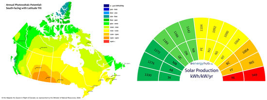
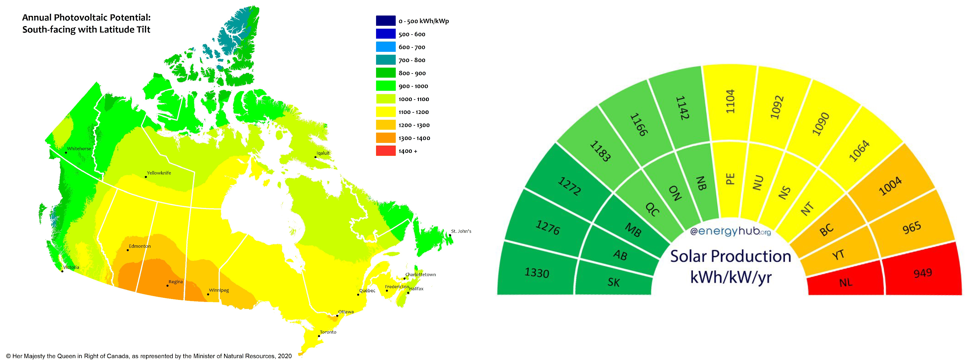
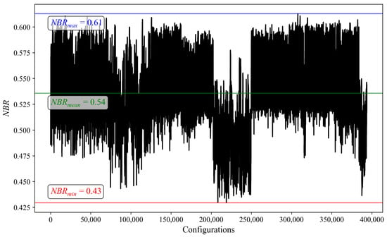
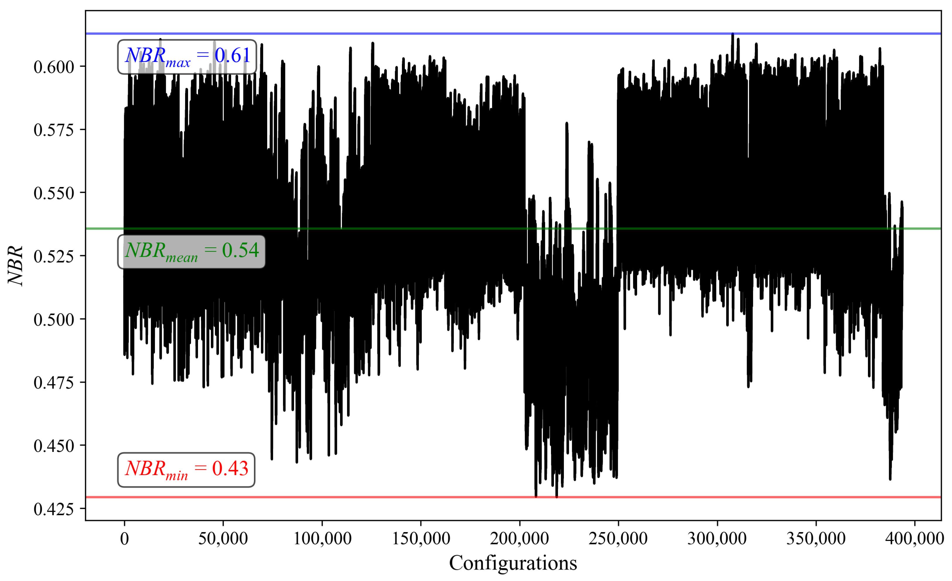
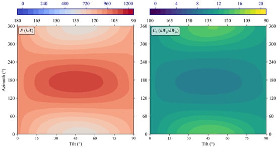
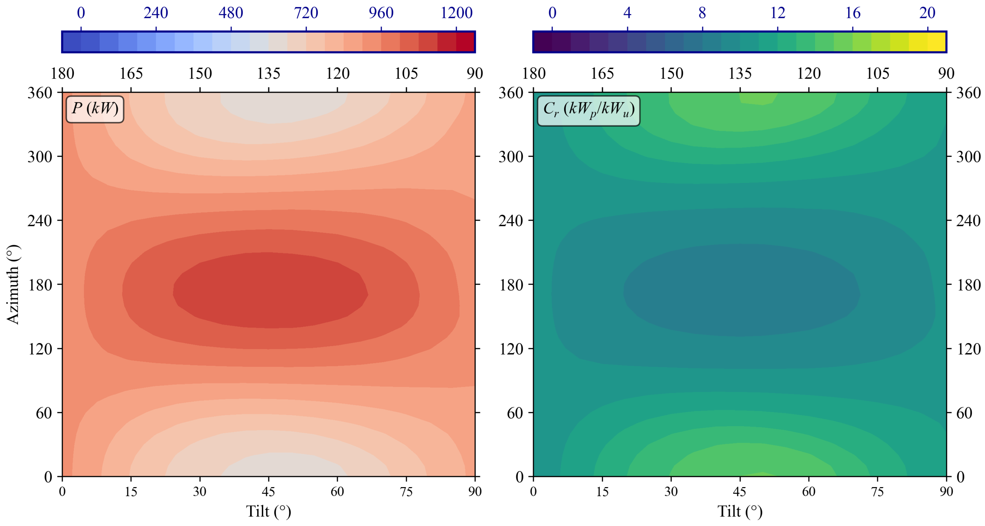
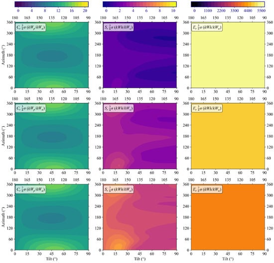
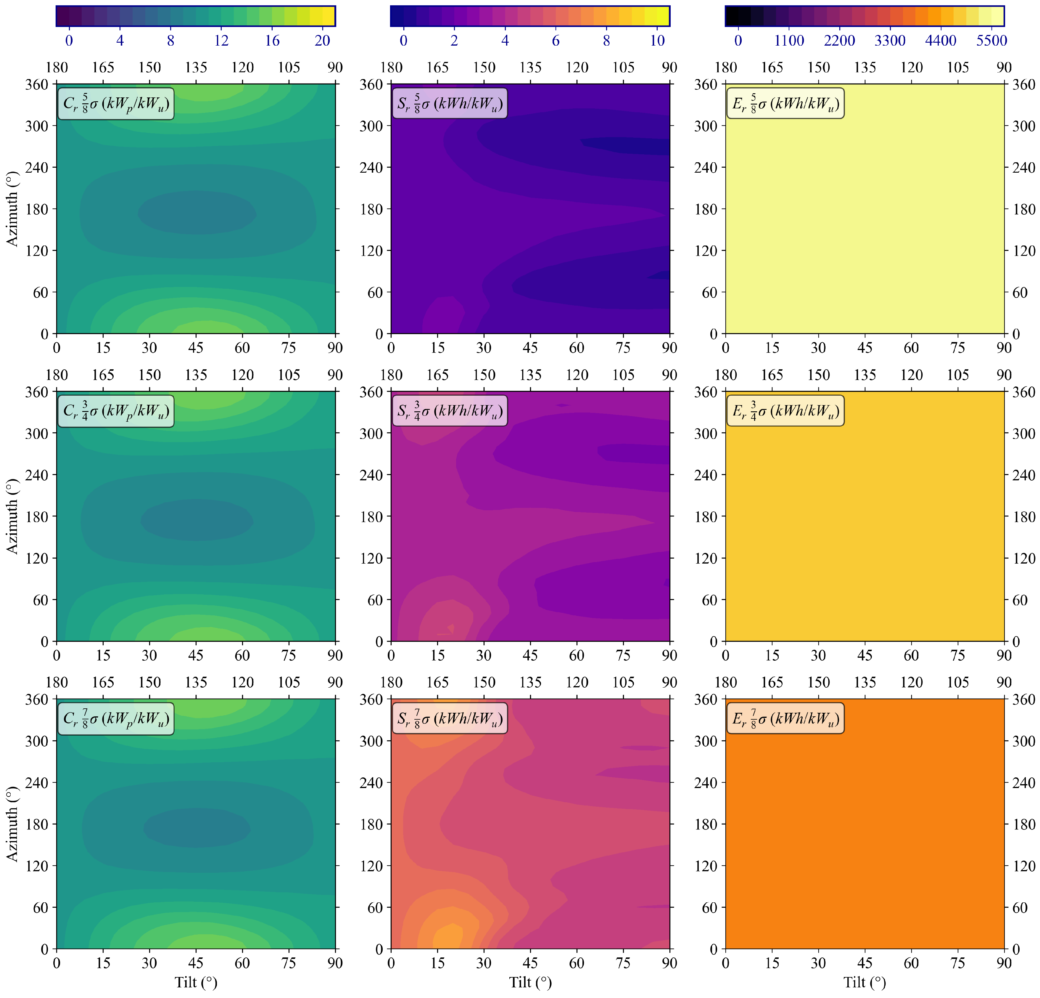
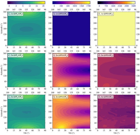
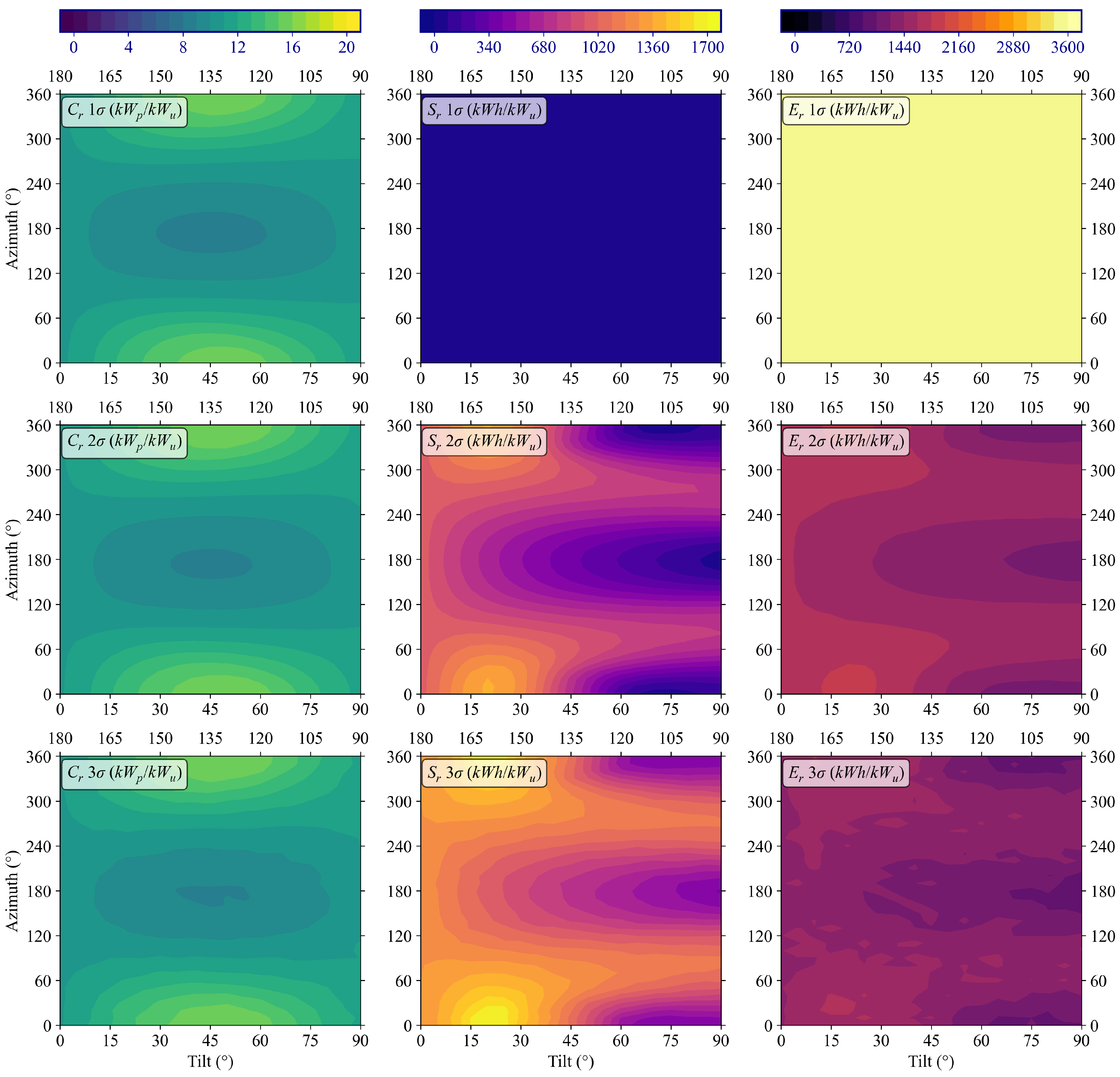
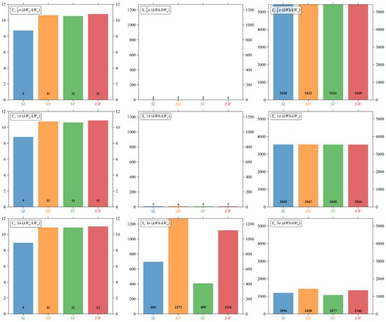
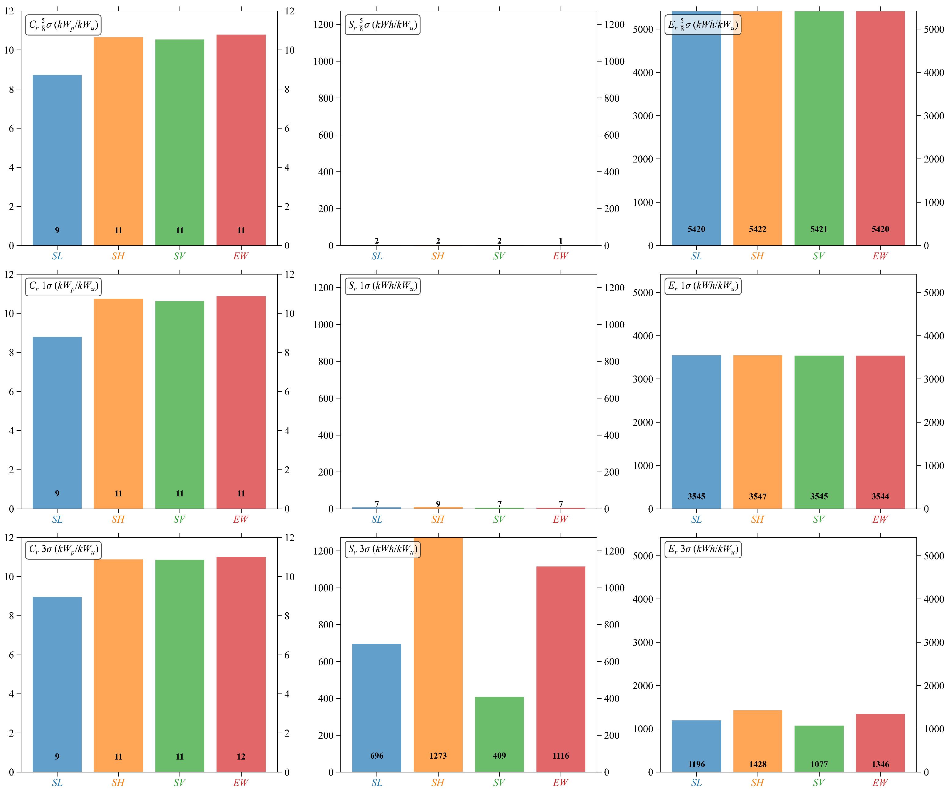
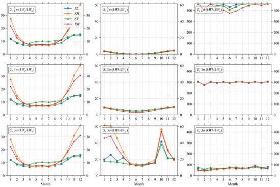
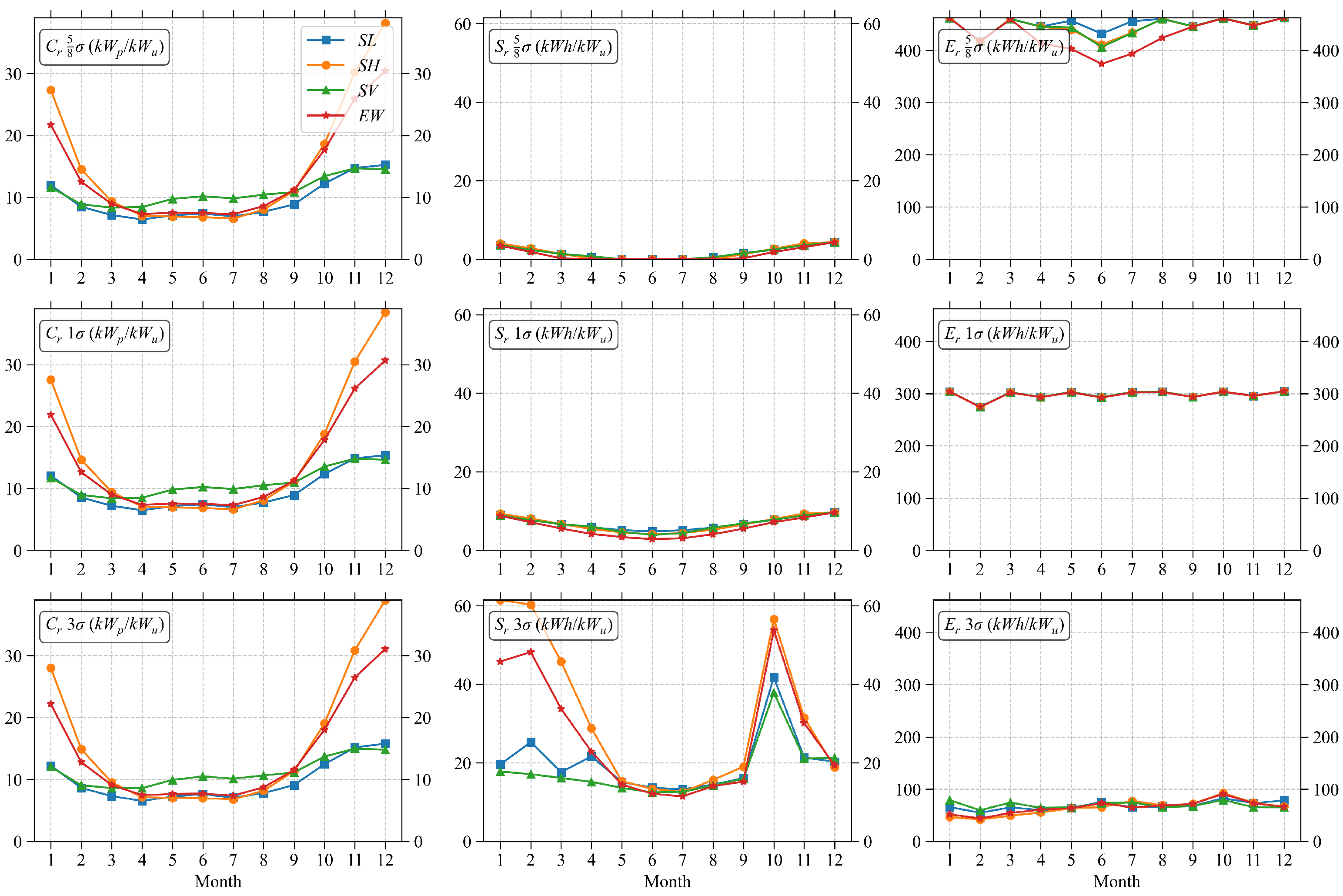
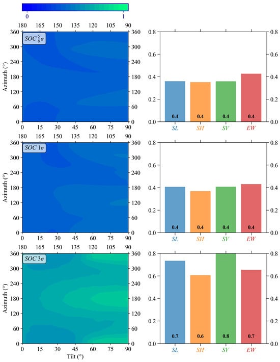
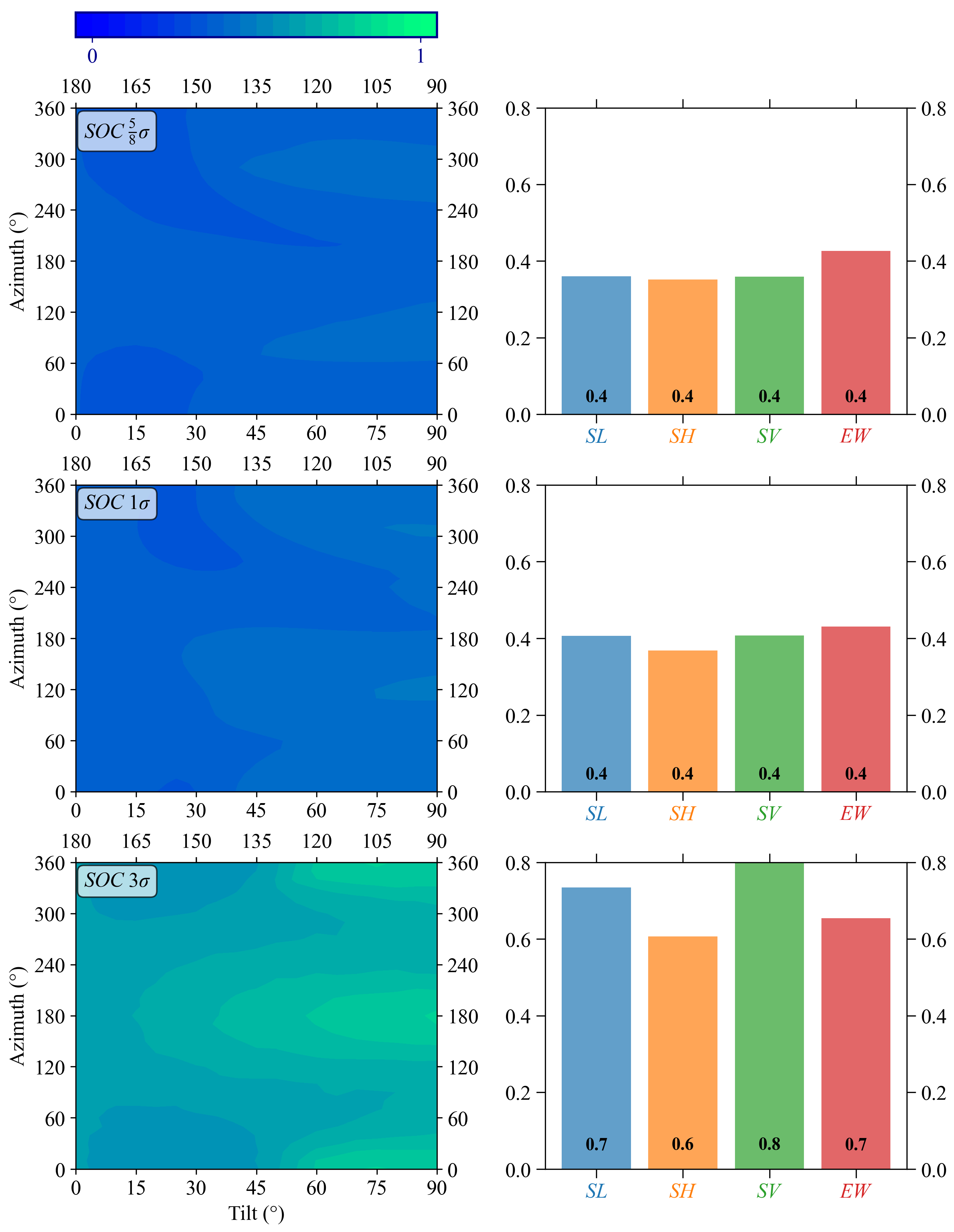
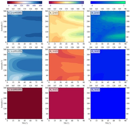
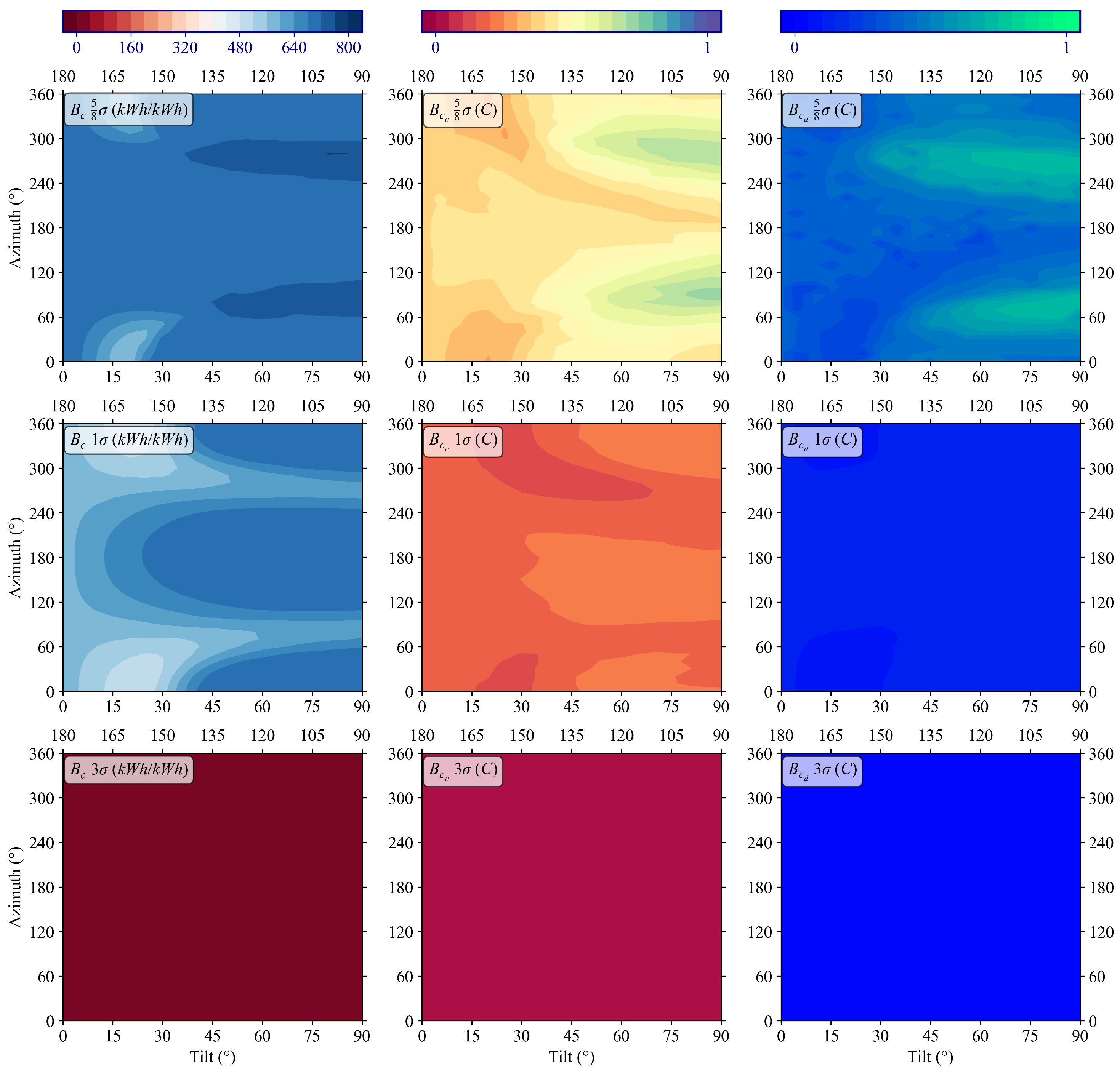
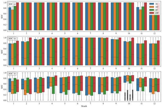
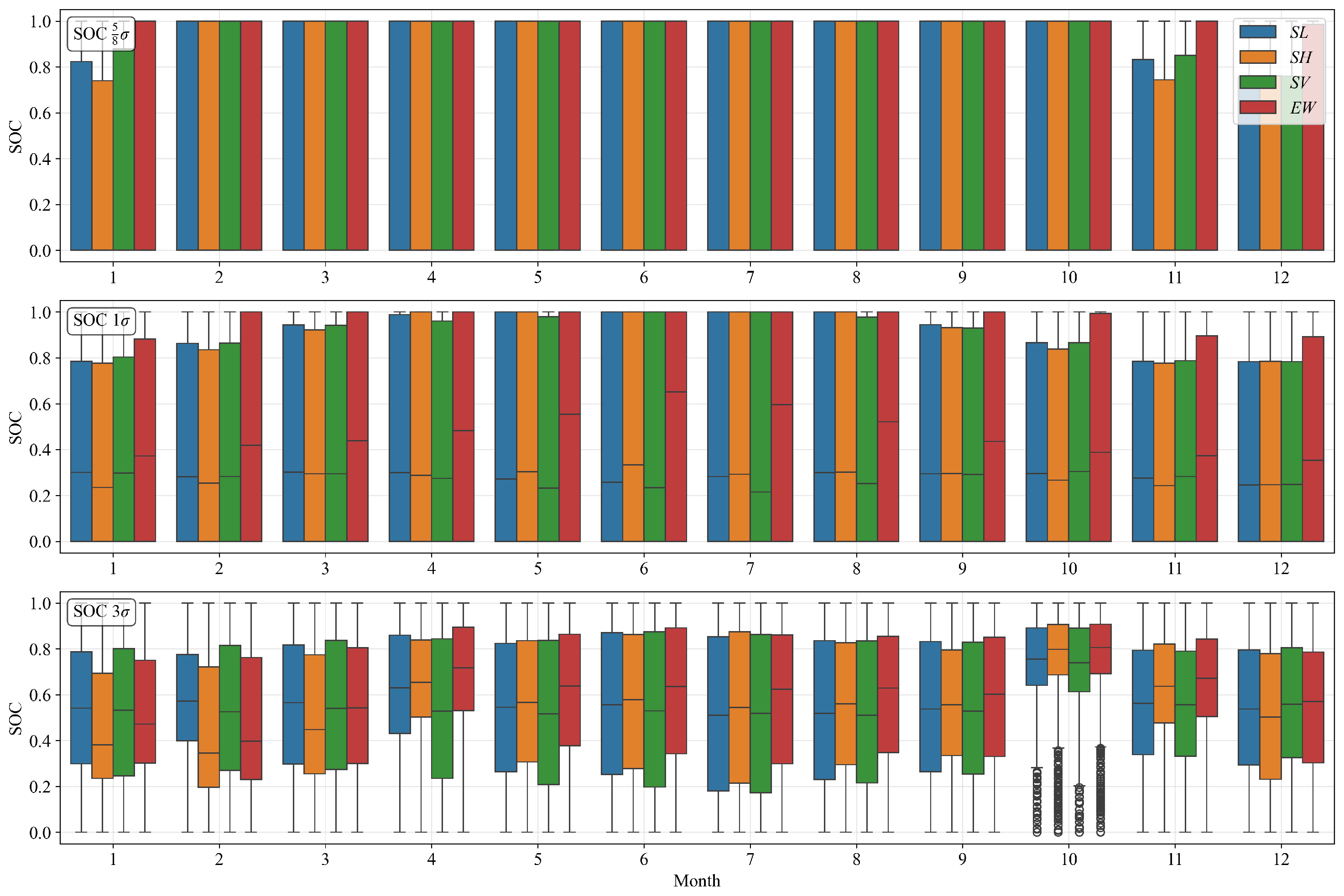
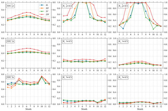
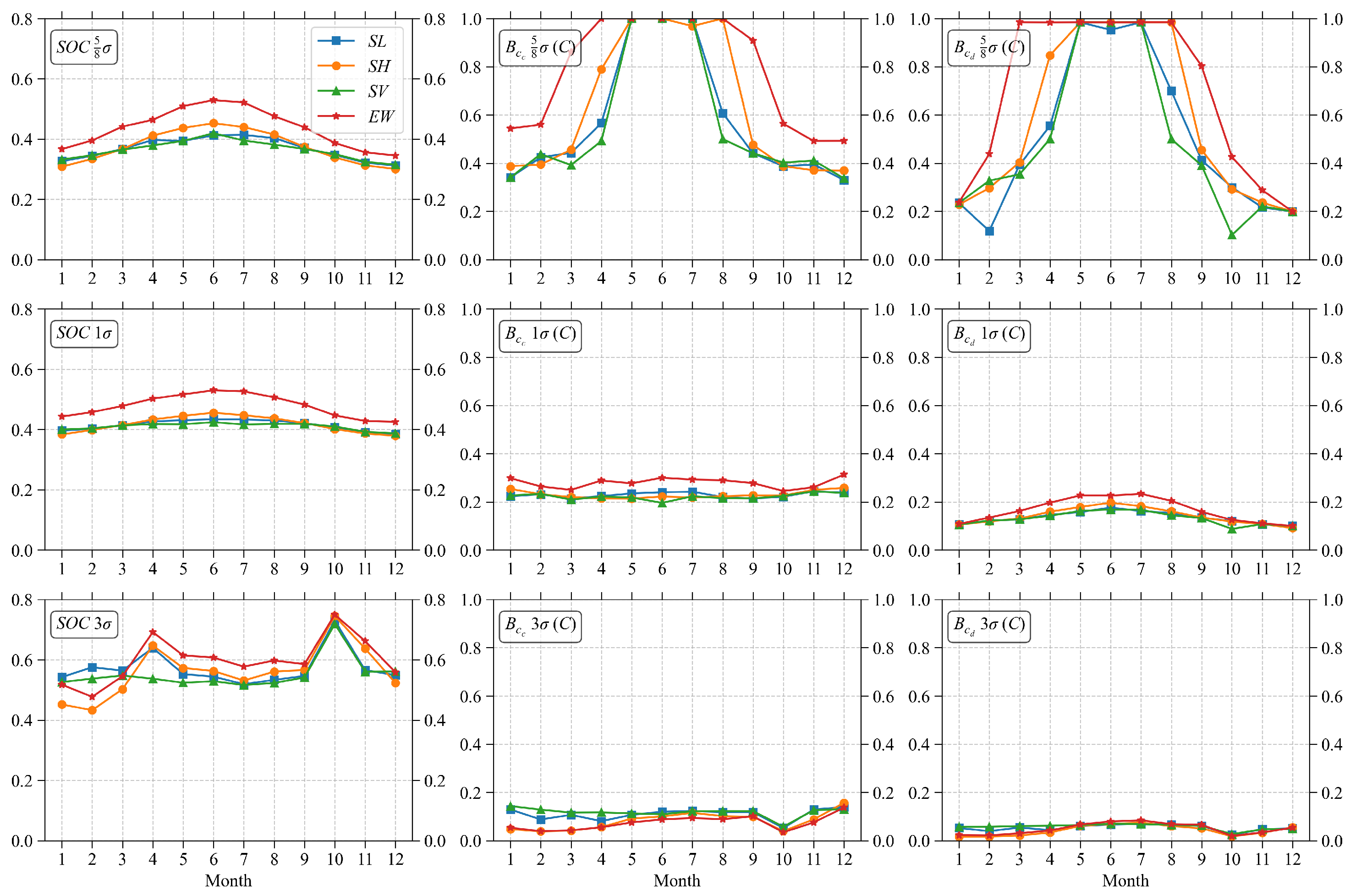
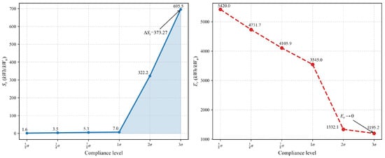
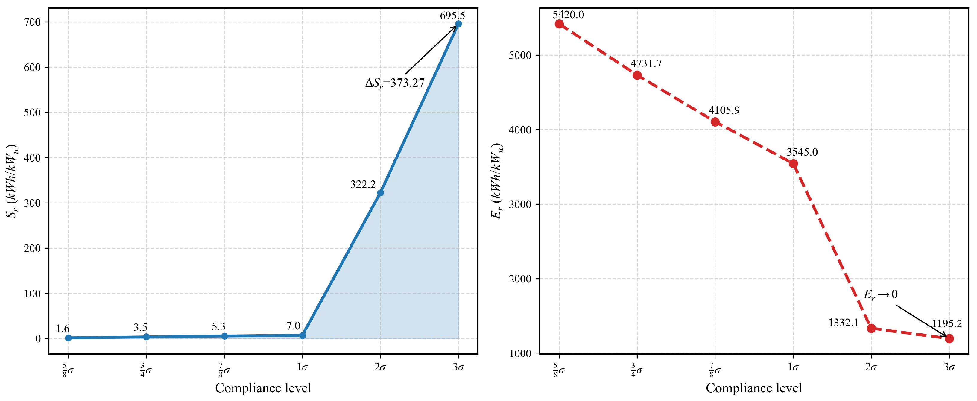
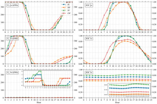
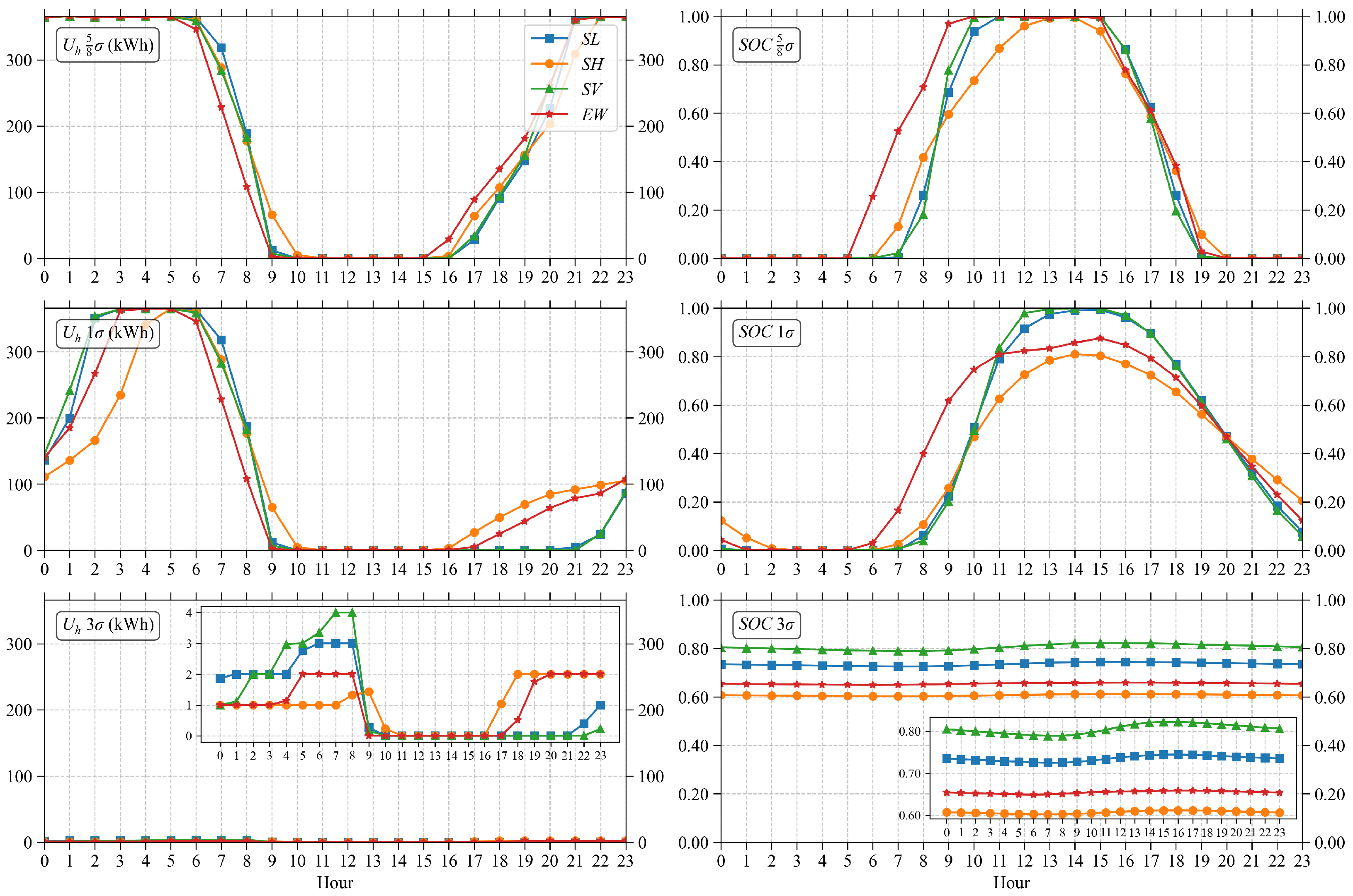

Disclaimer/Publisher’s Note: The statements, opinions and data contained in all publications are solely those of the individual author(s) and contributor(s) and not of MDPI and/or the editor(s). MDPI and/or the editor(s) disclaim responsibility for any injury to people or property resulting from any ideas, methods, instructions or products referred to in the content. |
© 2026 by the authors. Licensee MDPI, Basel, Switzerland. This article is an open access article distributed under the terms and conditions of the Creative Commons Attribution (CC BY) license.