


Abstract
Rail stations have non-traction electricity and heat demands, requiring coordinated renewable generation, storage, and conversion. We develop a cloud–edge–terminal energy-management framework for an electricity–hydrogen–thermal system. A 24 h mixed-integer linear programming model schedules grid import, photovoltaic (PV) generation, battery and thermal storage, electrolysis, hydrogen compression and storage, and fuel-cell and heat-pump operation. Hydrogen inventory is represented by stored hydrogen mass, with tank pressure linked to hydrogen density through a pressure–density relation. We compare three systems: hydrogen-free, hydrogen-integrated, and hydrogen-free with electrically equivalent battery storage. Hourly schedules map 150 capacity-equivalent virtual terminals for minute-level verification under operational and communication disturbances. Hydrogen integration reduces objective value by 1.06%, operating cost by 0.34%, and peak grid import by 6.89% relative to hydrogen-free operation but increases daily grid electricity purchase and CO2 emissions by approximately 3.09%. Sensitivity analyses show stronger benefits at higher PV penetration, negligible gains from tank-volume expansion beyond the storage range, and electrolyzer power as the constraint on renewable absorption at high PV capacities. Verification achieves a 98.503% average command–delivery success rate, a steady-state grid import error below 1 kW, and 2 min to self-heal faults. Hydrogen improves peak shaving and intertemporal energy shifting, whereas total electricity use and emissions depend on renewable availability and conversion limits.
1. Introduction
Rail stations are major energy-consuming facilities with substantial non-traction electrical and thermal demands. Lighting, ventilation, escalators, elevators, pumps, and air-conditioning systems contribute significantly to station-side energy use, and their demand varies with passenger flow, operating schedules, and environmental control requirements [1,2]. In this study, the rail station refers to the physical passenger service facility and its station-side energy infrastructure, while the energy hub represents the mathematical framework for coordinating multiple energy carriers and devices.
Integrated energy system approaches provide an effective framework for coordinating electricity, heat, hydrogen, and storage resources within rail station energy systems. By integrating renewable generation, energy conversion, and storage devices, integrated energy systems can improve operational flexibility compared with conventional single-energy supply structures [3,4]. The energy hub concept has been widely applied to represent interactions among different energy carriers and has been extended to multi-energy flow optimization and coordinated operation problems [5,6,7,8,9,10]. These characteristics make it suitable for rail stations with coupled electrical, thermal, and renewable energy resources.
Hydrogen can further enhance temporal energy-shifting capability by converting electricity into hydrogen through electrolysis, storing the hydrogen, and reconverting it into electricity and heat through fuel cells [11,12,13]. However, hydrogen integration introduces additional conversion losses, and its operational benefits depend on renewable availability, electricity-price structure, grid carbon intensity, equipment capacity, and dispatch strategy.
Existing studies have mainly focused on buildings, industrial parks, community microgrids, and other distributed-energy systems [11,12,13]. Rail stations have distinct non-traction load characteristics because HVAC and ventilation systems contribute substantial thermal demands [14]. Meanwhile, photovoltaic generation and battery storage have been investigated for metro and rail station applications [15,16]. However, the operational role of an electricity–hydrogen–thermal system under rail station non-traction load conditions remains insufficiently explored.
Another challenge lies in connecting day-ahead optimization with practical short-timescale operation. Cloud–edge and cloud–edge–terminal architectures have been introduced to improve distributed computation and real-time control capability in integrated energy systems and smart grids [17,18,19,20]. However, the coordination between electricity–hydrogen–thermal scheduling and short-term command execution under operational and communication disturbances has received limited attention.
The formulation used in this study extends existing energy hub and hydrogen-integrated models [21,22,23,24] to rail station non-traction energy management. A 24 h mixed-integer linear programming model is developed to coordinate electricity, hydrogen, and thermal energy flows, where hydrogen storage is represented by stored hydrogen mass and constrained through the tank pressure–density relationship. Three configurations are compared, including hydrogen-free, hydrogen-integrated, and hydrogen-free with an electrically equivalent BESS. Sensitivity analyses of hydrogen tank volume and PV capacity are conducted to evaluate the factors influencing hydrogen-system performance. The optimized schedules are further mapped to 150 capacity-equivalent virtual terminals for minute-level functional verification under representative disturbances [25,26,27].
The main contributions are summarized as follows. First, an existing energy hub formulation is extended to a rail station electricity–hydrogen–thermal system by incorporating hydrogen production, compression, mass-based storage, fuel-cell conversion, and heat recovery under non-traction load conditions. Second, the operational value of hydrogen integration is evaluated through comparisons with hydrogen-free and electrically equivalent BESS configurations, together with sensitivity analyses of storage volume and PV capacity. Third, a cloud–edge–terminal verification framework is applied to evaluate short-time command tracking and disturbance response using capacity-equivalent virtual terminals.
2. Materials and Methods
2.1. Energy-Flow Structure and Virtual-Terminal Simulation Setting
The system considered in this study supplies station-side non-traction electrical and thermal loads of a rail station. Traction power and train onboard auxiliary electricity are excluded from the modeling boundary. The electrical load represents station-service demand, including lighting, ventilation, escalators, elevators, and pumps, while the thermal load mainly represents HVAC and ventilation-related demand. The system includes grid supply, photovoltaic generation, battery storage, an electrolyzer, hydrogen storage, a fuel cell, a heat pump, and thermal storage.
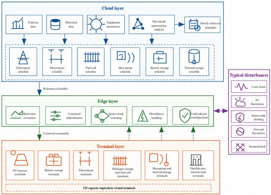
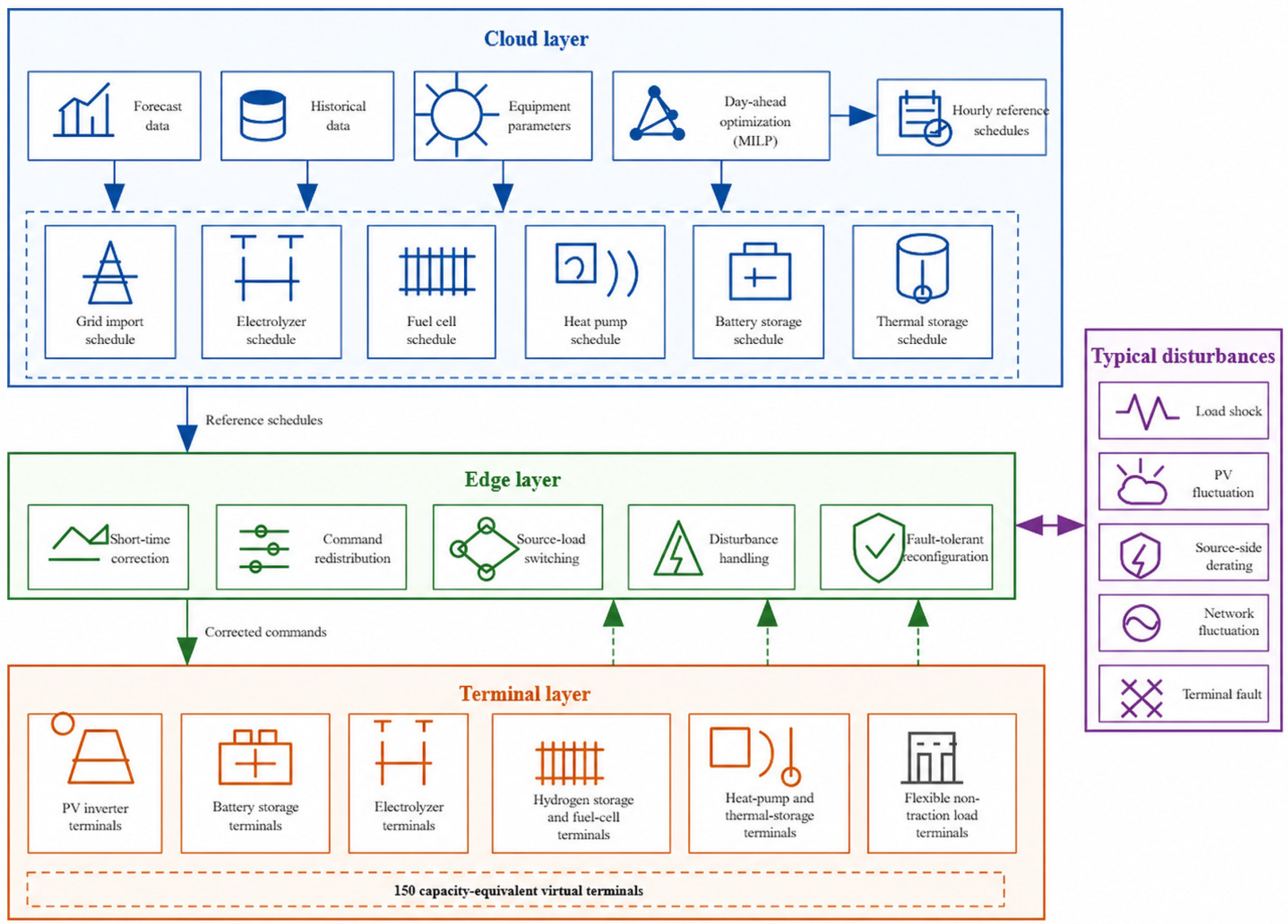
Figure 1 illustrates the cloud–edge–terminal structure developed for short-timescale energy-flow redistribution. At the cloud layer, a 24 h day-ahead optimization model generates hourly reference schedules for grid import, conversion devices, and storage units. These schedules are converted into 1 min reference commands at the edge layer. When disturbances occur, including load variation, photovoltaic fluctuation, source-side derating, network fluctuation, or terminal faults, the edge layer performs local command redistribution without re-optimizing the day-ahead model. Electrical deviations are compensated through available fuel-cell output, battery discharge, and flexible-load adjustment, while thermal deviations are regulated through coordinated heat-pump operation, fuel-cell heat recovery, and thermal storage.
Figure 1.
Simulation-oriented virtual-terminal setting for short-timescale energy-flow redistribution under typical disturbances.
The corrected commands are allocated to 150 capacity-equivalent virtual terminals according to controllable capacity and availability. If a terminal becomes unavailable, its allocation weight is redistributed among remaining terminals. Terminal states and measurements are returned to the edge layer for subsequent correction. The virtual terminals are used for simulation-based functional verification while maintaining the aggregated capacities and load boundaries defined in the cloud-layer optimization model.
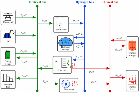
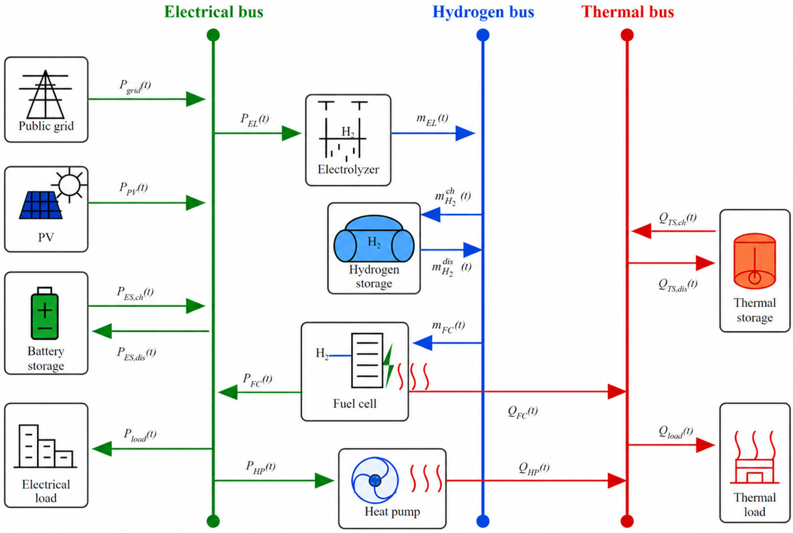
Figure 2 presents the corresponding electricity–hydrogen–thermal energy-flow structure. The grid and photovoltaic power supply the electrical bus, while the electrolyzer, fuel cell, heat pump, and three storage systems provide energy conversion and time-shifting among the electrical, hydrogen, and thermal subsystems.
Figure 2.
Energy-flow representation of the electricity–hydrogen–thermal energy hub serving non-traction loads at a rail station, including battery, hydrogen, and thermal storage.
2.2. Energy Hub Representation
The rail station system is represented as an energy hub because it contains coupled electrical, hydrogen, and thermal energy flows connected by conversion and storage devices. The public grid and photovoltaic system supply the electrical bus directly. The electrolyzer converts electricity into hydrogen, the fuel cell reconverts hydrogen into electricity and heat, and the heat pump converts electricity into heat. Battery, hydrogen, and thermal storage provide time-shifting capability for their respective energy carriers. This representation retains the conversion and storage pathways required for system-level dispatch without introducing a detailed physical network model.
For a single energy conversion process, the relationship between the input and output energy carriers can be expressed as follows:
where is the input energy of carrier α at time , is the output energy of carrier at time , and is the conversion efficiency from carrier to carrier . In the proposed system, this relationship describes the energy conversion processes of the electrolyzer, fuel cell, and heat pump.
The multi-energy input–output relationship of the electricity–hydrogen–thermal hub can be further written in a compact matrix form as
where , denote the input electrical power, equivalent hydrogen energy flow, and thermal power, respectively, and denote the corresponding output energy flows. is the coupling matrix of the energy hub, containing the conversion efficiencies and dispatch relationships among electricity, hydrogen, and heat.
In this study, the energy hub model is used as a system-level representation rather than a detailed physical network model. Detailed device models, energy balance equations, storage constraints, and the coordinated dispatch objective are presented in Section 2.3.
2.3. Cloud-Layer Day-Ahead Optimization Model
The mathematical formulation of the proposed energy-management model is developed based on the established energy hub framework for integrated energy systems. Previous studies have widely applied mixed-integer optimization formulations to coordinate renewable generation, energy conversion devices, and storage units in multi-energy systems [5,6,7,8,9,10]. Following these formulations, this study focuses on the operational coordination of a rail station electricity–hydrogen–thermal system by incorporating a pressure-dependent hydrogen storage representation and short-timescale cloud–edge–terminal verification.
At the cloud layer, a 24 h day-ahead dispatch model with a 1 h time step is formulated using electrical and thermal loads, photovoltaic output, electricity prices, prescribed equipment parameters, and initial storage states. The model generates hourly reference schedules for grid import, conversion devices, and storage units for subsequent edge-layer operation.
The model optimizes operational dispatch under fixed equipment capacities; therefore, capacity expansion and investment decisions are not considered. This treatment is adopted because this study focuses on evaluating the short-term operational coordination of an existing rail station integrated energy system rather than determining the optimal investment scale of each energy asset. Including capital expenditure would require additional assumptions regarding equipment lifetime, replacement cycles, discount rates, and investment constraints, which would transform the problem into a long-term capacity planning problem. Accordingly, capital expenditure (CAPEX) is excluded from the objective function. The objective function focuses on daily operational performance, including grid electricity purchase cost, carbon emission cost, and peak-load penalty terms under the specified system configuration. Therefore, the obtained objective value represents short-term operational performance rather than a life-cycle economic evaluation or investment-feasibility metric.
The objective function minimizes the comprehensive operating objective
where is the electricity purchase cost from the public grid, is the operation and maintenance cost of system devices, is the carbon emission cost, is the photovoltaic curtailment penalty, and is the peak grid import penalty.
The grid electricity purchase cost is calculated as
where is the time-of-use electricity price at time , is the grid import power, is the dispatch time interval, and is the total number of dispatch intervals.
The operation and maintenance cost is expressed as
where are the operation and maintenance cost coefficients of the electrolyzer, fuel cell, heat pump, battery storage, hydrogen storage, and thermal storage, respectively.
The carbon emission cost is given by
where is the carbon price, and is the carbon emission factor of grid electricity.
The photovoltaic curtailment penalty is calculated as
where is the photovoltaic curtailment penalty coefficient, is the available photovoltaic output, and is the absorbed photovoltaic power.
The peak grid import penalty is defined as
where is the peak penalty coefficient, and is the maximum grid import power during the dispatch period.
The electricity balance constraint is written as
where is the electrical load demand, is the electrical input of the electrolyzer, is the electrical input of the heat pump, is the electrical output of the fuel cell, is the electrical consumption of the hydrogen compression process, and and are the charging and discharging powers of the battery storage, respectively.
The thermal energy balance constraint is given by
where is the thermal output of the heat pump, is the thermal output of the fuel cell, is the thermal load demand, and and are the charging and discharging thermal powers of the thermal storage unit, respectively.
The electrolyzer converts electrical power into hydrogen mass flow, which is described as
where is the conversion efficiency of the electrolyzer, and represents the lower heating value of hydrogen.
The fuel cell converts hydrogen energy into electricity and heat, expressed as
where and are the electrical and thermal efficiencies of the fuel cell, respectively, and represents the hydrogen mass consumed by the fuel cell at time .
The electricity consumption of the hydrogen compression process is considered separately from the electrolyzer efficiency. A linear compression energy model is adopted, which is expressed as
where is the linear compression energy coefficient.
The heat pump converts electrical power into thermal power according to
where is the coefficient of performance of the heat pump.
The state of charge of the battery storage is described as
where is the stored electrical energy, and and are the charging and discharging efficiencies of the battery storage, respectively.
The hydrogen storage mass balance is described as
where represents the hydrogen mass stored in the storage tank at time , and and denote the hydrogen charging and discharging mass flows, respectively.
To account for the physical limitation imposed by the hydrogen storage vessel, the stored hydrogen mass is related to the tank internal volume and hydrogen density according to
where is the total internal geometric volume of the hydrogen storage vessels, and is the hydrogen density corresponding to the tank operating pressure.
Because hydrogen exhibits non-ideal gas behavior at high pressure, the relationship between hydrogen density and storage pressure is obtained from NIST real-gas property data under the prescribed storage temperature. To maintain the mixed-integer linear structure of the day-ahead optimization model, the pressure–density relationship is approximated using a piecewise linear function over the operating pressure range of 12.3–35 MPa.
The piecewise linear approximation provides sufficient accuracy for representing pressure-dependent hydrogen storage characteristics while preserving the computational tractability of the MILP formulation.
The hydrogen storage pressure is constrained by
where is the tank pressure, and and are the minimum and maximum allowable operating pressures, respectively.
The thermal storage state is expressed as
where is the stored thermal energy, and and are the charging and discharging efficiencies of the thermal storage unit, respectively.
The operating limits of the main devices are defined as
The storage capacity constraints are given by
To avoid simultaneous charging and discharging of the storage units, binary variables are introduced as follows:
Similar constraints are applied to hydrogen storage and thermal storage:
where and are binary variables that prevent simultaneous charging and discharging of the corresponding storage units.
The peak grid import variable is constrained by
where represents the maximum grid import power over the entire dispatch horizon. Through this formulation, the proposed model can coordinate electricity purchase, photovoltaic utilization, hydrogen production and reconversion, heat supply, and storage operation under multiple technical and economic constraints.
2.4. Edge-Layer Real-Time Coordination Control
The edge layer receives the operating references issued by the cloud optimization layer and performs real-time power adjustment according to the local load, PV output, and device operating states. The net power deviation between the actual operating condition and the cloud-layer reference is calculated as
where indicates that the actual net load exceeds the cloud-layer reference and additional local regulation is required. When , no upward power compensation is activated, and the deviation is reflected in the grid exchange power.
To characterize the gradual recovery of a failed device, a fault self-healing coefficient is introduced. During the recovery process, takes values of 0, 0.15, 0.35, 0.60, and 1 from the fault occurrence to full recovery. The coefficient is used to modify the available regulation capability of the affected device.
At each control interval, the edge layer evaluates the available regulation capacity according to the current operating point, stored energy or hydrogen mass, device availability, and fault recovery state. For the fuel cell, the maximum hydrogen consumption rate supported by the current hydrogen storage state is
where is the stored hydrogen mass. According to the fuel-cell hydrogen-to-electricity conversion model established in Section 2.3, the corresponding maximum electrical output is
where denotes the fuel-cell power conversion relationship defined in Section 2.3. The available additional fuel-cell regulation capacity is therefore expressed as
The maximum additional discharge capacity of the BESS is
and the maximum flexible-load curtailment capacity is
where denote the availability states of the fuel cell, BESS, and flexible load, respectively, and is the regulation reserve coefficient. These constraints ensure that the regulation command remains within the physically available operating range of each resource.
When , the power deviation is compensated sequentially by the fuel cell, BESS discharge, and flexible load curtailment:
The remaining uncompensated power is calculated as
To prevent abrupt changes in device commands, the adjusted power is further constrained by the ramping capability of each resource:
where k represents the fuel cell, BESS, or flexible load, and (R_k) is the maximum allowable power variation within one edge-layer control interval.
After the local adjustment, the actual grid exchange power is calculated as
and the tracking error relative to the cloud-layer reference is defined as
The actual device powers obtained after local regulation are subsequently used to update the BESS, hydrogen storage, and thermal storage states. In particular, the hydrogen storage state is represented by the stored hydrogen mass and updated according to the electrolyzer hydrogen production and fuel-cell hydrogen consumption defined in Section 2.3. The thermal balance also accounts for the heat supplied by the heat pump and the recoverable heat from the fuel cell.
For a device group containing multiple terminal units, the group-level command is distributed among the available devices in proportion to their rated capacities as follows:
where denotes the set of available terminal devices in group g at control interval m, and is the rated capacity of terminal device i. Through this coordination mechanism, the edge layer corrects the cloud-layer schedule according to real-time operating conditions and distributes the adjusted group-level commands to individual terminal devices.
3. Case Study and Scenario Definition
3.1. Input Data and Model Parameters
The case study represents a literature-calibrated synthetic typical day for a large rail station under the climatic and electricity-market conditions of Sichuan Province, China. The input profiles are reconstructed rather than measured data from a specific station, using published station-energy studies [14,15,28,29], meteorological and photovoltaic resources [30,31], time-of-use tariff documents [32,33], and the official grid-emission factor [34].
The non-traction electrical load profile is derived from published station-operation measurements excluding train-traction demand [14,15,28]. The normalized hourly profile is scaled according to the reported energy-use intensity of Chinese underground stations [28]. Heat-pump electricity is excluded from the exogenous electrical load because it is determined by the dispatch model. The thermal load profile represents HVAC service demand and is reconstructed from published subway station HVAC studies [28,29].
Solar and meteorological data for Chengdu are obtained from NASA POWER [30], and the photovoltaic profile is calculated using PVWatts and scaled to an installed capacity of 250 kW [31]. This capacity is used as a reference setting for operational analysis rather than an optimal sizing result; the effect of PV capacity is examined separately in Section 4.3. The electricity tariff follows the Sichuan peak-flat-valley structure, with a flat-period price of 0.70 CNY/kWh and a price ratio of 1.6:1.0:0.4 [32,33]. The grid carbon emission factor is taken from the official provincial dataset [34]. Equipment capacities and efficiencies are specified according to the modeled load level and published integrated energy system studies [11,12], as summarized in Table A1.
For the case study, hydrogen equipment is assumed to be located in a dedicated area separated from passenger zones, with ventilation, leak detection, pressure relief, fire protection, and emergency shutdown. Detailed siting and quantitative safety assessment are outside the scope of this study.
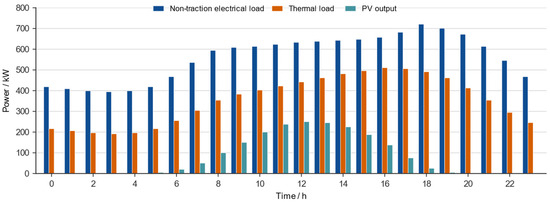
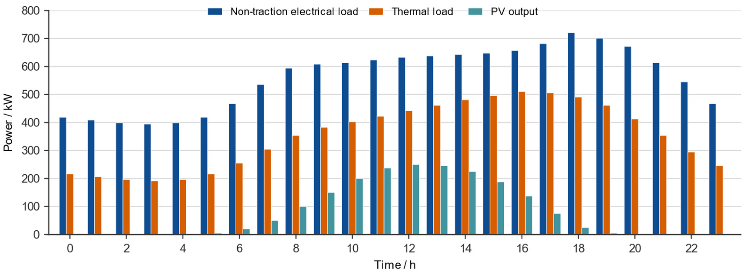
As shown in Figure 3, non-traction electrical demand dominates the daily load, while thermal demand remains significant. PV output is concentrated during daytime and provides limited support during the evening high-load period, forming the operating basis for the subsequent hydrogen-integration analysis.
Figure 3.
Baseline profiles of non-traction electrical load, thermal load, and photovoltaic output.
The cloud-layer dispatch is solved over a 24 h horizon with a 1 h interval. The technical, economic, and storage-state parameters are summarized in Table A1. The model is implemented in MATLAB R2026a using YALMIP version 20250626 and solved with the intlinprog solver.
For the hydrogen-free and hydrogen-integrated scenarios, the electrical and thermal load profiles, PV profile, electricity tariff, carbon emission factor, and common equipment parameters are kept identical. In the sensitivity analyses, only the parameter under investigation is varied while the remaining settings are unchanged.
3.2. Scenario Definition
Three system-configuration scenarios are defined to evaluate the operational effects of hydrogen integration, as summarized in Table 1. The hydrogen-free scenario includes the public grid, PV system, battery storage, heat pump, and thermal storage. The hydrogen-integrated scenario retains the same baseline components and additionally incorporates an electrolyzer, hydrogen compressor, pressurized hydrogen storage tank, and fuel cell. A hydrogen-free scenario with an equivalent BESS is also considered an additional benchmark for evaluating the system-level flexibility provided by hydrogen storage. All three scenarios use identical electrical and thermal load profiles, PV generation profiles, electricity tariffs, carbon emission factors, and common equipment parameters. Configuration-specific storage parameters are varied only where required by the corresponding scenario.
Table 1.
Scenario settings.
The three scenarios are compared in terms of the objective value, operating cost, grid electricity purchase, peak grid import power, and carbon emissions. The equivalent-BESS scenario is used as a system-level flexibility benchmark and does not imply complete technological equivalence between battery and hydrogen storage systems.
Sensitivity analyses are conducted separately for the hydrogen storage tank volume and installed PV capacity. For the hydrogen-integrated configuration, the hydrogen storage tank volume is varied from 10% to 150% of the baseline value, corresponding to approximately 0.258–3.87 m3, with a reference volume of 2.58 m3. The allowable tank pressure range is fixed at 12.3–35 MPa, while the initial and terminal tank pressures are maintained at approximately 15.7 MPa to ensure a consistent cyclic operating condition. For the PV-capacity sensitivity analysis, the installed PV capacity is varied from 0 to 1500 kWp in increments of 250 kWp by proportionally scaling the normalized daily generation profile. During each sensitivity analysis, only the parameter under investigation is varied, while all other model parameters and corresponding terminal-state constraints remain unchanged.
Platform-oriented functional verification is conducted separately. The 24 h reference dispatch from the hydrogen-integrated reference case is held fixed and mapped to 150 capacity-equivalent virtual terminals for a selected hour. Load shocks, photovoltaic fluctuations, source derating, source-load switching, network fluctuations, and terminal faults are then imposed to evaluate short-time command redistribution and execution. This is a simulation-based verification rather than measurement-based hardware-platform validation.
4. Results and Discussion
4.1. Comparison of the Hydrogen-Free and Hydrogen-Integrated Scenarios
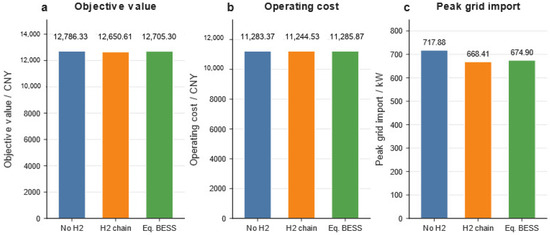
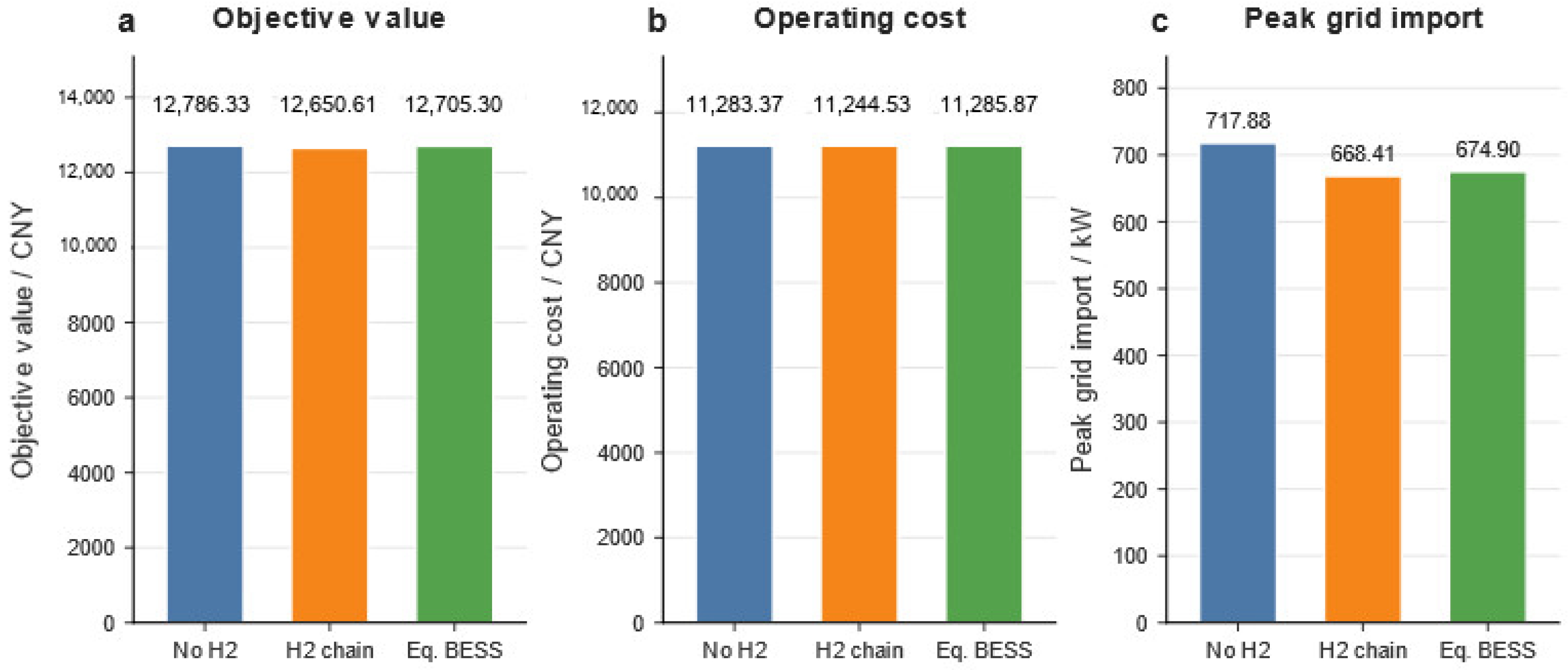
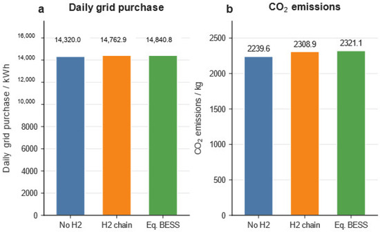
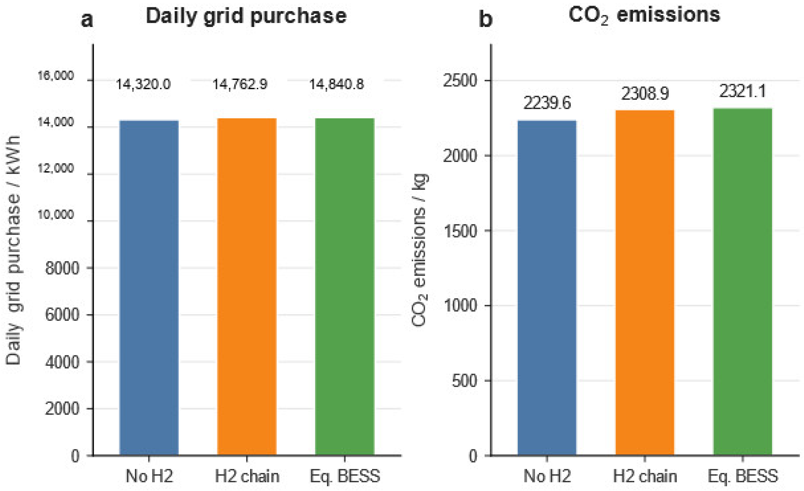
As described in Section 3.2, three system configurations are evaluated using the reconstructed input dataset: the hydrogen-free scenario, the hydrogen-integrated scenario, and the hydrogen-free scenario with an electrically equivalent BESS. The comparison focuses on day-ahead operational dispatch under predefined equipment capacities. The objective function includes grid-purchase and equipment-operation-and-maintenance costs, together with carbon emission and peak-load penalty terms. Capital expenditures are not included. The resulting objective value therefore represents the operational performance of the three configurations rather than their life-cycle cost or investment return. Figure 4 and Figure 5 compare the objective value, operating cost, peak grid import, daily grid electricity purchase, and CO2 emissions.
Figure 4.
Comparison of the objective value, operating cost, and peak grid import between the hydrogen-free and hydrogen-integrated scenarios.
Figure 5.
Comparison of daily grid electricity purchase and CO2 emissions between the hydrogen-free and hydrogen-integrated scenarios.
Figure 4 shows that the hydrogen-integrated scenario achieved the lowest objective function value, operating cost, and peak grid import among the three scenarios. Relative to the hydrogen-free scenario, the objective function value and operating cost decreased by 1.06% and 0.34%, respectively, while the peak grid import decreased from 717.88 to 668.41 kW, representing a reduction of 6.89%. The electrically equivalent battery energy storage system (BESS) scenario also provided peak-shaving benefits; however, its objective function value, operating cost, and peak grid import remained higher than those of the hydrogen-integrated scenario. These results indicate that hydrogen storage enhances the intertemporal flexibility of system dispatch and improves peak-load management.
The hydrogen subsystem remained within its prescribed physical operating limits throughout the scheduling horizon. The hydrogen tank pressure ranged from 15.684 to 24.502 MPa, and the electrolyzer produced 13.8545 kg of hydrogen. During operation, the compressor consumed 41.5636 kWh of electricity, whereas the fuel cell delivered 207.7972 kWh of electricity and 161.6200 kWh of thermal energy. Collectively, these results demonstrate the role of the electricity–hydrogen–electricity/heat conversion pathway in reallocating stored energy to periods of higher system demand.
Figure 5 shows that the hydrogen-free scenario resulted in the lowest grid electricity purchase and CO2 emissions. Relative to this scenario, hydrogen integration increased both indicators by approximately 3.09%. This increase is consistent with the additional electricity required for electrolysis and hydrogen compression, together with the conversion losses associated with hydrogen utilization. Nevertheless, compared with the electrically equivalent BESS scenario, the hydrogen-integrated scenario reduced both grid electricity purchase and CO2 emissions by approximately 0.53%.
Taken together, the hydrogen-integrated scenario achieved the lowest objective function value, operating cost, and peak grid import among the three scenarios and performed better than the electrically equivalent BESS scenario across the assessed indicators. Under the operating conditions considered here, the principal benefit of hydrogen integration appears to arise from enhanced dispatch flexibility and peak-shaving capability rather than from a reduction in total grid electricity consumption. These findings highlight the distinction between the operational and energy-consumption benefits of hydrogen storage.
4.2. Typical Daily Time-Series Operation Analysis
The time-series results provide mechanistic insight into the peak-shaving behavior observed in Section 4.1. For the reference configuration with an installed PV capacity of 250 kW, the electrolyzer produced hydrogen, which was subsequently compressed and stored before being consumed by the fuel cell to supply electricity and recoverable heat. Accordingly, the hydrogen inventory was represented directly by the stored hydrogen mass, consistent with the revised mass-based storage formulation.
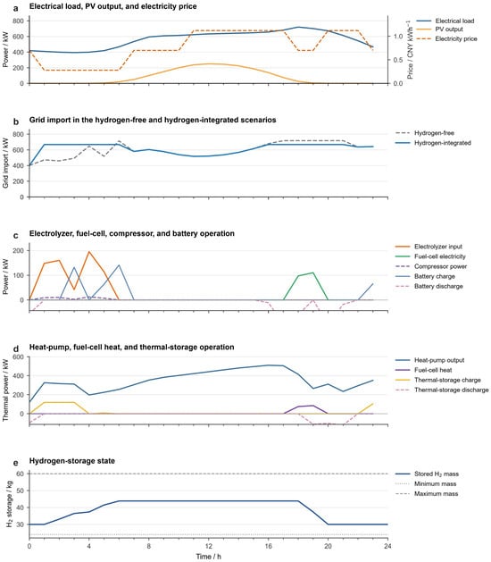
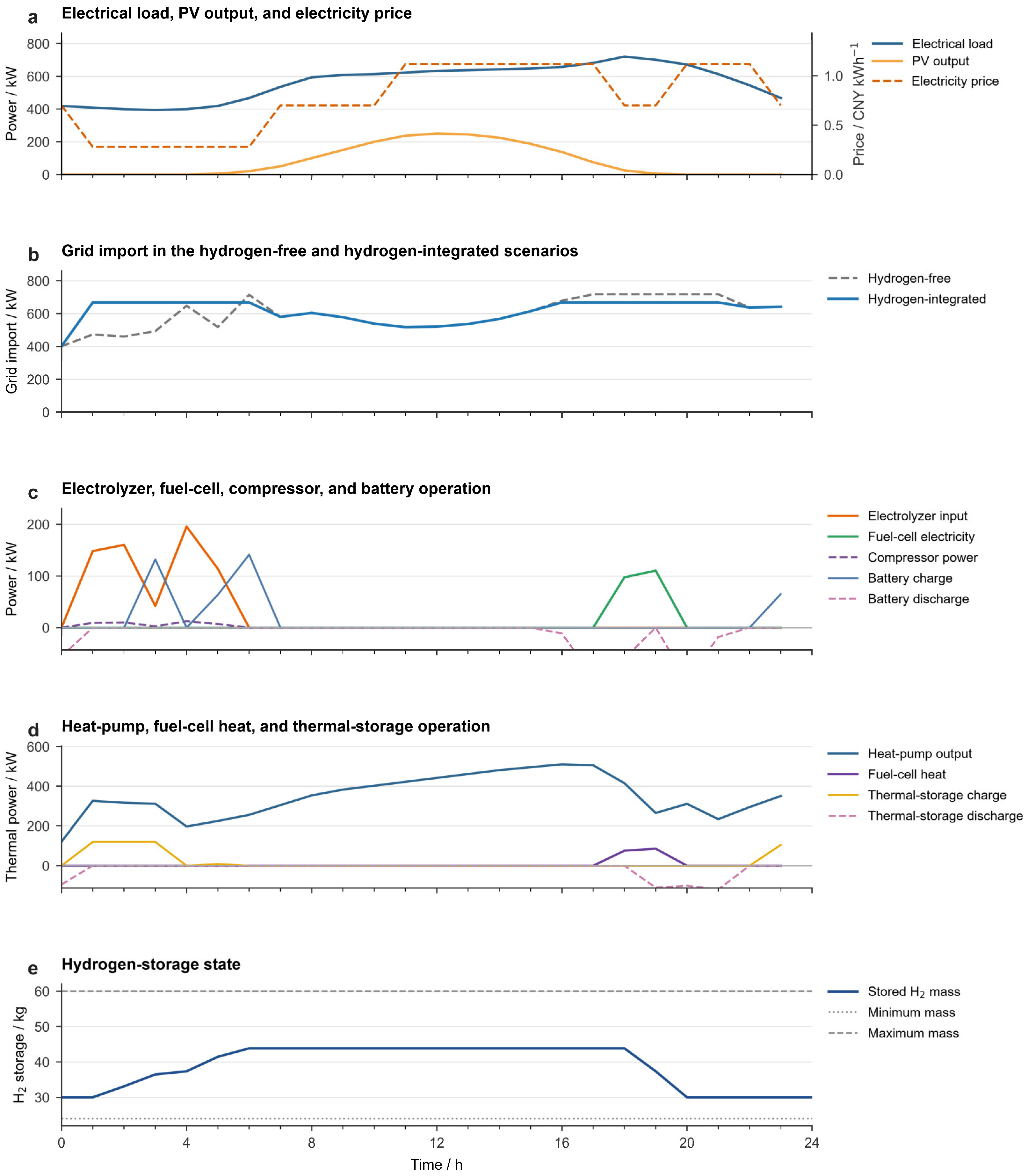
Figure 6 depicts the time-resolved operating sequence of the hydrogen-integrated configuration. During the initial low-price period, the electrolyzer was scheduled to produce hydrogen, while the compressor imposed a modest additional electricity demand. Consequently, grid import temporarily exceeded that of the hydrogen-free configuration, whereas the stored hydrogen mass increased from approximately 30 to 44 kg. The accumulated hydrogen was subsequently retained for use during higher-price periods. This scheduling strategy shifted part of the electricity consumption to lower-price hours and preserved stored hydrogen for subsequent fuel-cell operation.
Figure 6.
Typical daily operation of grid import, hydrogen-chain power, and hydrogen storage state under the hydrogen-integrated scenario with the reference parameter settings.
During the evening period, which was characterized by high electricity prices and system load, the electrolyzer remained idle, and the stored hydrogen was dispatched to the fuel cell. The fuel cell simultaneously supplied electricity and recoverable heat, thereby reducing both grid electricity imports and heat-pump demand. Consequently, the maximum grid import decreased from 717.88 kW in the hydrogen-free configuration to 668.41 kW in the hydrogen-integrated configuration, corresponding to a reduction of 6.89%.
The hydrogen conversion chain therefore reshaped the grid import profile through intertemporal energy shifting. Additional electricity was consumed for hydrogen production during the low-price period, whereas the stored hydrogen was subsequently converted back into electricity and heat during the later high-demand period. This coordinated operation reduced the original grid import peak and resulted in a flatter import profile. Battery and thermal storage provided short-term balancing for the electrical and thermal subsystems, whereas hydrogen storage supported energy shifting over a longer time horizon.
As shown in Figure 6e, the stored hydrogen mass increased from approximately 30 to 44 kg during the hydrogen-production period and subsequently declined to approximately 30 kg when the fuel cell operated. The hydrogen inventory remained within its prescribed minimum and maximum limits throughout the scheduling horizon and returned to its initial level by the end of the day. This terminal condition supports the interpretation that the observed peak-shaving effect resulted from the temporal redistribution of energy rather than from net depletion of the hydrogen inventory. Overall, the hydrogen conversion chain primarily enhanced peak-shaving capability and operational flexibility by shifting energy from low-price periods to subsequent periods of high demand.
4.3. Sensitivity Analysis
Sensitivity analyses were conducted for hydrogen tank volume and installed PV capacity. Unless otherwise specified, the load profiles, electricity tariff, carbon emission factor, equipment efficiencies, peak grid import penalty coefficient, and other operating parameters were kept unchanged. For the hydrogen tank volume analysis, the pressure limits and temperature were fixed, while the hydrogen mass bounds and initial and terminal storage states were recalculated consistently with the pressure–density relationship for each tank volume.
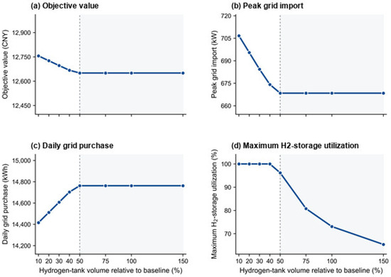
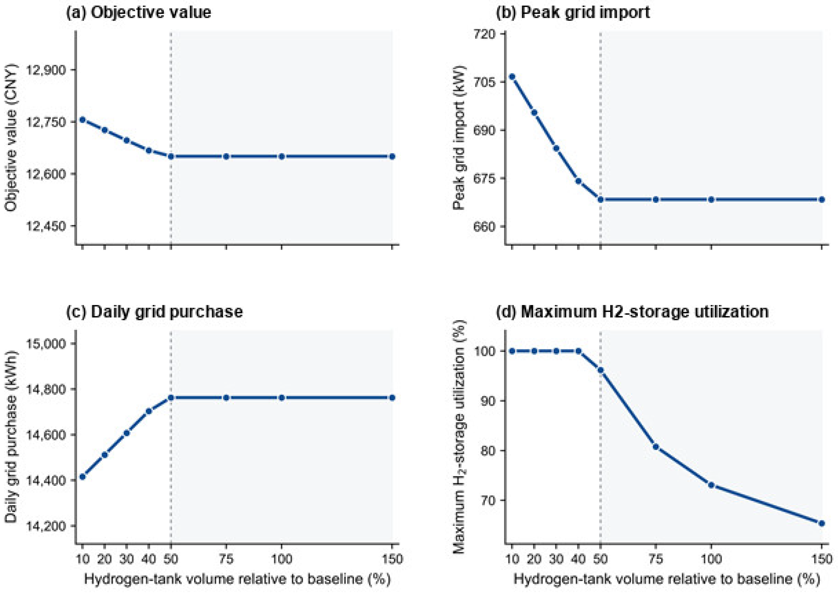
As shown in Figure 7, increasing the hydrogen tank volume from 10% to 50% of the baseline value improved the overall operating performance of the system. The objective function value decreased from 12,756.39 to 12,650.61 CNY, while peak grid import declined from 706.70 to 668.41 kW, corresponding to reductions of 0.83% and 5.42%, respectively. Over the same range, daily grid electricity purchase increased from 14,415.88 to 14,762.89 kWh. This increase occurred because the larger storage capacity allowed more electricity to be converted into hydrogen and subsequently reconverted by the fuel cell, thereby introducing additional conversion losses. Nevertheless, the resulting intertemporal energy shifting reduced peak grid demand and the overall objective function value.
Figure 7.
Sensitivity of system performance to hydrogen tank volume.
A clear saturation point emerged at approximately 50% of the baseline tank volume. Below this threshold, the maximum hydrogen storage utilization remained close to 100%, indicating that storage capacity acted as an active operational constraint. Beyond this threshold, the objective function value, peak grid import, and daily grid electricity purchase remained essentially unchanged, whereas the maximum storage utilization decreased continuously. These results indicate that increasing the tank volume beyond approximately 50% provided no additional operational benefit under the considered PV-generation and load conditions. Therefore, approximately 50% of the baseline tank volume was sufficient to avoid storage-capacity limitations in the investigated system.
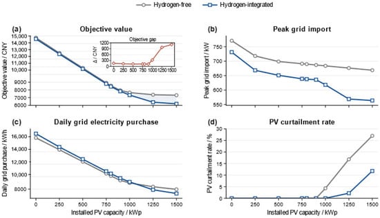
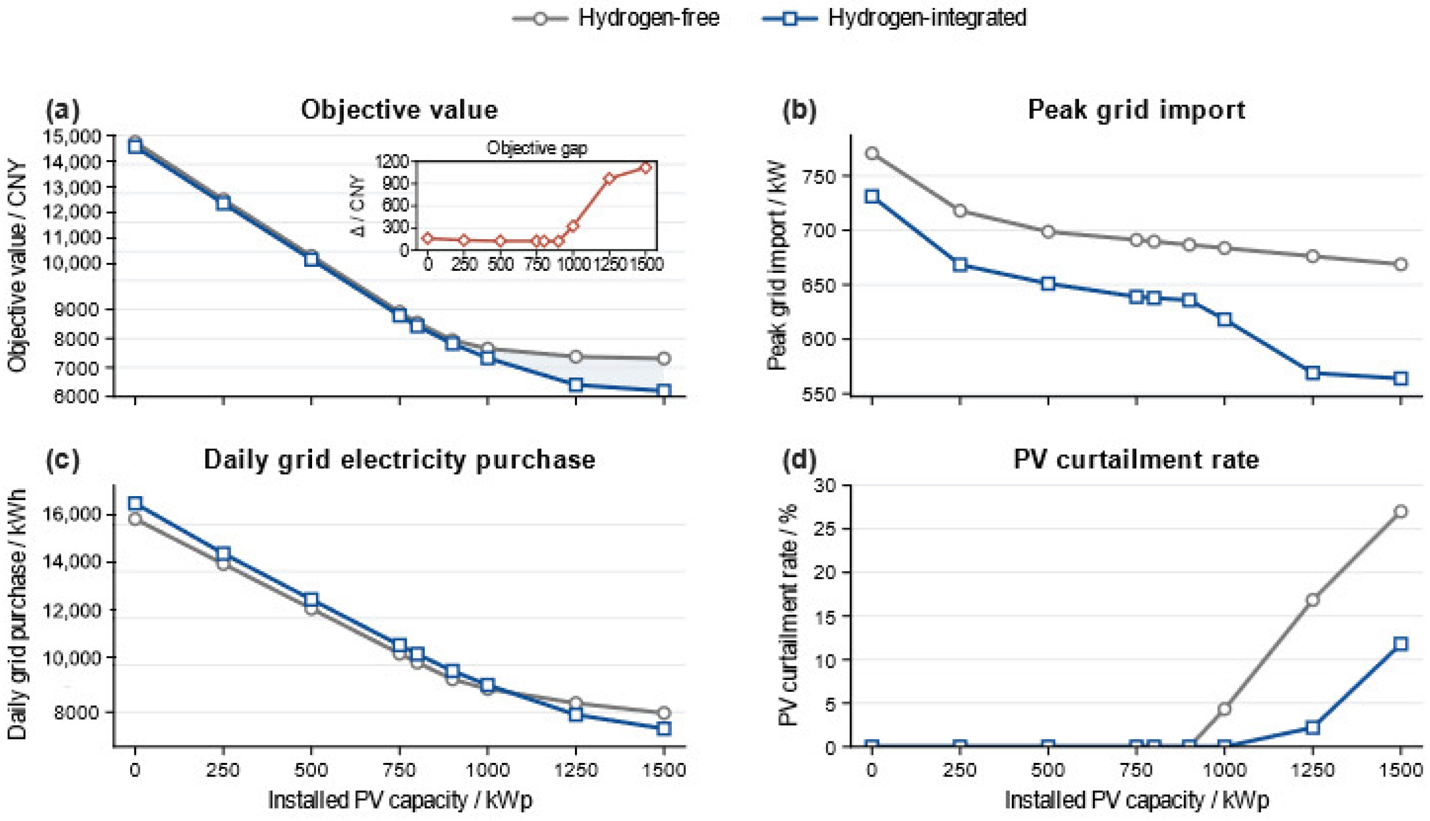
To investigate the influence of PV penetration on system performance and the operational value of the hydrogen chain, the installed PV capacity was varied from 0 to 1500 kWp in increments of 250 kWp. At each capacity level, the hydrogen-free and hydrogen-integrated configurations were optimized under identical load profiles, electricity tariffs, equipment parameters, and terminal-state constraints. The resulting changes in objective value, peak grid import, daily grid electricity purchase, and PV curtailment rate are presented in Figure 8.
Figure 8.
Sensitivity analysis of system performance to PV capacity.
The sensitivity analysis presented in Figure 8 shows that the operational role of the hydrogen chain changes as renewable energy penetration increases. Increasing the installed PV capacity progressively reduces both the objective function value and the peak grid import in the hydrogen-free and hydrogen-integrated configurations. At low PV capacities of 0–750 kWp, the difference between the two configurations remains limited because most PV generation can be consumed directly by the electrical loads, leaving relatively little surplus electricity for hydrogen production. When the PV capacity reaches 1000 kWp or higher, the objective-function gap widens rapidly, indicating that hydrogen integration becomes increasingly valuable when renewable generation exceeds the system’s direct consumption capacity.
The trend in daily grid electricity purchase further clarifies the changing operational role of hydrogen. At low PV capacities, the hydrogen-integrated configuration requires slightly more grid electricity because the electrolyzer operates mainly during periods of limited PV availability and therefore relies partly on grid-supplied electricity. Additional conversion losses are also introduced through the hydrogen pathway. As the PV capacity increases, surplus PV generation becomes available for hydrogen production, thereby reducing the system’s dependence on grid electricity. Consequently, the hydrogen-integrated configuration achieves lower daily grid electricity purchase than the hydrogen-free configuration at higher PV capacities. Meanwhile, the reduction in peak grid import provided by hydrogen becomes increasingly pronounced, indicating enhanced peak-shaving capability under higher renewable energy penetration.
PV curtailment highlights the limitation of further increasing the installed PV capacity. In the hydrogen-free configuration, curtailment begins to occur at 1000 kWp and increases rapidly with additional PV capacity. By contrast, the hydrogen-integrated configuration effectively avoids curtailment at 1000 kWp by converting surplus PV generation into hydrogen. Curtailment nevertheless emerges at 1250 kWp and increases to 11.80% at 1500 kWp. The operational analysis indicates that this increase is mainly attributable to the electrolyzer’s rated-power limitation, as the electrolyzer reaches its maximum input power during periods of high PV availability. Thus, hydrogen integration can substantially improve PV utilization and reduce grid dependence; however, its capacity to absorb additional renewable generation remains constrained by the rated capacity of the hydrogen conversion subsystem.
4.4. Platform-Oriented Functional Verification
The previous sections evaluate the cloud-layer dispatch result at the system level. To further connect the hourly schedule with terminal-level execution, a platform-oriented functional verification is carried out. This part does not change the 24 h optimization result; instead, it checks whether the aggregated cloud-layer schedules can be decomposed into terminal commands and corrected by the edge layer under short-time disturbances. Since complete physical communication logs are not available, the verification is interpreted as a simulation-oriented test based on capacity-equivalent virtual terminals rather than a hardware experiment.
According to the virtual-terminal decomposition and command-allocation procedure described in Section 2.1, the aggregated cloud-layer energy-flow objects are mapped to 150 capacity-equivalent virtual terminals for short-timescale functional verification. The terminal configuration is summarized in Table 2. The decomposition preserves the total device capacities and load boundaries of the cloud-layer model and therefore does not alter the objective value, energy balance, or day-ahead dispatch result.
Table 2.
Multi-terminal configuration for platform-oriented verification.
A fixed population of 150 capacity-equivalent virtual terminals is adopted as the predefined terminal scale for the platform-oriented simulation. The terminal number is treated as a simulation-setting parameter rather than an optimized system-design variable or the actual number of physical devices in a specific rail station. The decomposition is used to represent distributed command allocation and terminal availability while preserving the aggregated capacities and energy-flow boundaries of the cloud-layer model.
4.4.1. Verification Scenarios and Performance Indicators
The short-timescale verification is conducted for the representative 18:00–19:00 interval of the hydrogen-integrated case. During this period, the electrical and thermal loads are 720.519 and 491.046 kW, respectively, while the available PV output is 25.000 kW. The electrolyzer is inactive, and the fuel cell provides electrical and thermal support using stored hydrogen.
The hourly cloud-layer schedule is used as the reference command, and the edge-layer correction is simulated at a 1 min resolution. An electrical load disturbance and a temporary PV reduction are imposed during the interval. The fuel cell adjusts its output accordingly, while the hydrogen storage mass decreases from 43.858 to 36.078 kg and the tank pressure decreases from 23.985 to 19.202 MPa. The disturbance settings are summarized in Table 3.
Table 3.
Minute-level disturbance settings for platform-oriented verification during 18:00–19:00.
Under these disturbances, the edge layer follows a priority-based correction rule. On the electrical side, additional deficits are first compensated by fuel-cell support, then by battery discharge, and finally by flexible non-traction load adjustment. On the thermal side, heat-pump output, fuel-cell heat recovery, and thermal storage are coordinated to reduce thermal imbalance. The verification indicators include command–delivery success rate, synchronization delay, grid import tracking error, terminal load rate, capacity margin, unmet command, response time, and fault self-healing time.
4.4.2. Short-Timescale Verification Results
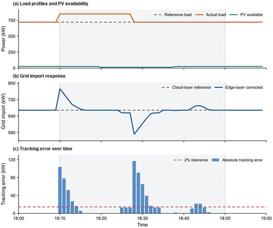
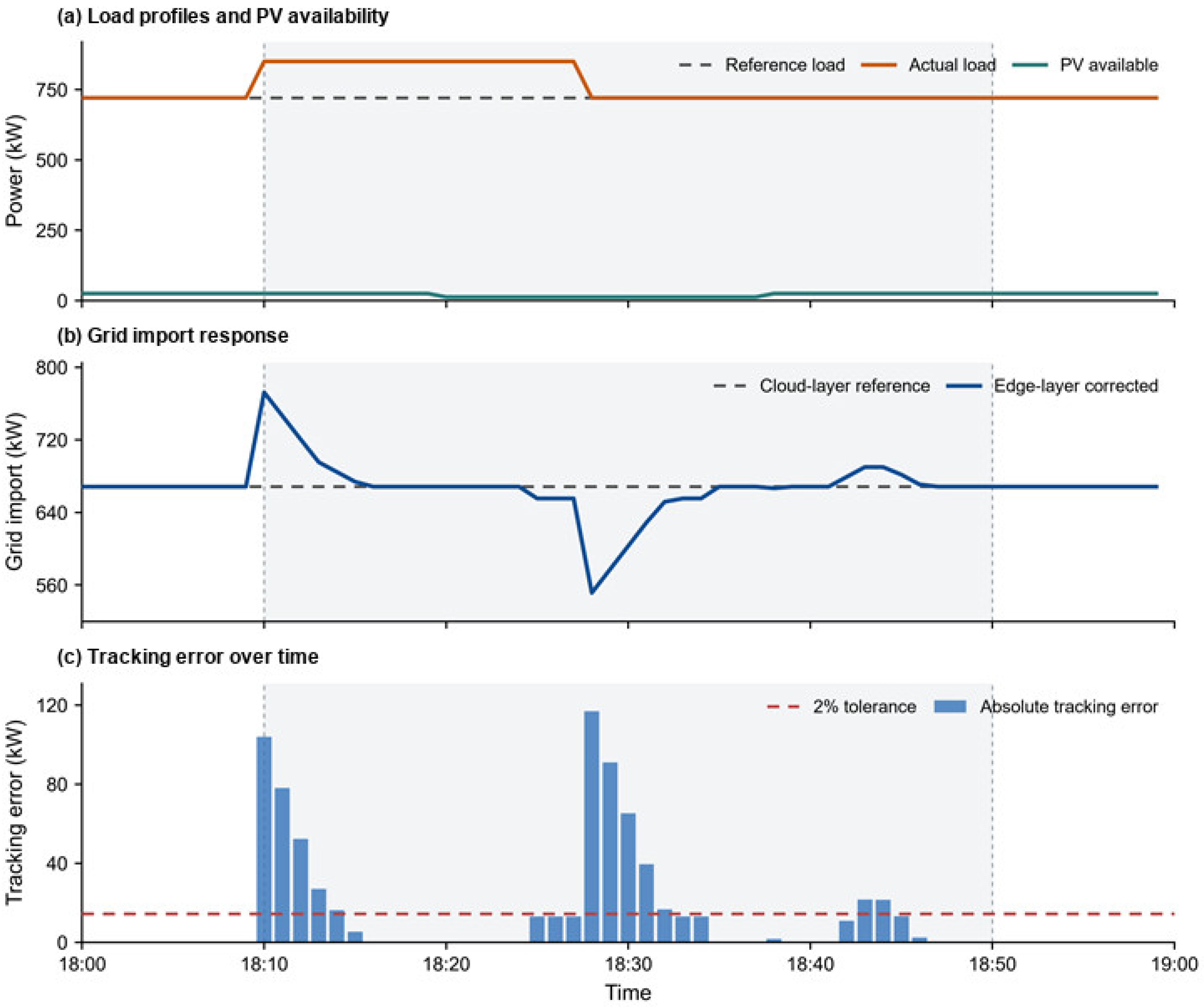
Figure 9 presents the minute-level response of the edge layer under combined load and PV disturbances. As shown in Figure 9a, the electrical load temporarily increased above its hourly reference level, followed by a reduction in available PV output. These changes produced overlapping short-term disturbances. In response, the edge layer adjusted grid import away from the cloud-layer reference, as shown in Figure 9b, and progressively restored it as the disturbances subsided. A brief deviation in the opposite direction was also observed during the load-recovery period, reflecting the transient redistribution of power among the available devices.
Figure 9.
Minute-level grid import response under combined disturbances during 18:00–19:00.
Figure 9c shows that the 2% tracking threshold was temporarily exceeded, primarily around the onset and removal of the disturbances. During the subsequent steady-state periods, the tracking error remained relatively small. Overall, these results indicate that the edge layer can respond effectively to minute-level fluctuations and steer system operation back towards the hourly cloud-layer reference following short-term disturbances.
The nonzero tracking error is accompanied by a maximum terminal load rate of 99.570% and a minimum capacity margin of 0 kW, confirming that the deviation is mainly caused by insufficient regulation capacity during overlapping disturbances.
Table 4 summarizes the performance of the minute-level platform-oriented verification. The 150 virtual terminals achieved an average command–delivery success rate of 98.503%, while the minimum success rate was 85.167%. The average synchronization delay was 0.323 s, and the maximum delay was limited to 2.000 s. The load-disturbance response time was 5 min, whereas the steady-state tracking error remained below 1 kW (<0.1%).
Table 4.
Performance metrics of the minute-level platform-oriented verification.
The maximum grid import tracking error reached 116.870 kW, corresponding to 16.220% of the reference value. Meanwhile, the maximum and average terminal load rates were 99.570% and 68.090%, respectively, and the minimum capacity margin was 0 kW. The maximum unmet power and total unmet energy were 103.893 kW and 5.875 kWh, respectively. The combination of near-maximum terminal loading, zero minimum capacity margin, and nonzero unmet power indicates that the available regulation resources approached their capacity limits during the verification process. Source–load switching achieved a success rate of 60.000%, and the fault self-healing process was completed within 2 min. These results characterize the performance of the virtual-terminal platform under minute-level platform-oriented verification.
5. Conclusions
Overall, this study developed a coupled electricity–hydrogen–thermal energy-flow model with mass-based hydrogen storage and pressure–density coupling for rail station energy management. Compared with the hydrogen-free configuration, hydrogen integration reduced the total objective function value by 1.06%, the operating cost by 0.34%, and the peak grid import by 6.89%. However, daily grid electricity purchase and carbon emissions increased by 3.09%. These results indicate that, under the considered PV capacity, tariff structure, grid carbon factor, and conversion efficiencies, hydrogen integration primarily improves peak-shaving capability and intertemporal dispatch flexibility rather than directly reducing total electricity consumption or carbon emissions.
The sensitivity analyses further clarify the operating conditions under which hydrogen integration is most beneficial. Increasing PV capacity reduced grid dependence and peak grid import, while the relative advantage of hydrogen integration became more pronounced when surplus PV generation exceeded the direct consumption capacity of the system. At high PV capacities, PV curtailment increased because the electrolyzer reached its rated input-power limit. Increasing the hydrogen tank volume improved the objective function value and peak grid import up to approximately 50% of the baseline volume. Further expansion produced negligible operational benefits under the considered PV and load conditions, indicating that the system was constrained primarily by conversion power, load profiles, and renewable energy availability rather than by storage volume.
Minute-level virtual-terminal verification showed that the proposed framework could coordinate hourly schedules under short-term disturbances. The platform controlled 150 virtual terminals, achieved an average command–delivery success rate of 98.503%, maintained a steady-state tracking error below 1 kW, and completed fault self-healing within 2 min. These results support the feasibility of the proposed hierarchical scheduling and disturbance–response framework for dispatch-level coordination.
Several limitations remain. The input profiles were reconstructed representative scenarios rather than measured station data, and the virtual-terminal verification was simulation-based because complete physical platform and communication records were unavailable. The current model also simplifies detailed compressor dynamics, transient hydrogen pressure behavior, equipment degradation, multi-day uncertainty, and rolling re-optimization. In addition, equipment capacities were predefined, so capacity planning, capital expenditure, and life-cycle economic performance were not evaluated. Future work should incorporate measured station data, detailed device-level dynamics, dynamic carbon factors, and multi-day rolling dispatch.
Author Contributions
Conceptualization, J.Y. (Juncheng Yang), S.X., X.Z. and G.W.; methodology, J.Y. (Juncheng Yang); software, J.Y. (Juncheng Yang); validation, J.Y. (Juncheng Yang), G.G., J.L. (Junhao Liang) and D.Y.; formal analysis, J.Y. (Juncheng Yang) and J.L. (Junhao Liang); investigation, J.Y. (Juncheng Yang), J.Y. (Jie Yan), D.Y. and J.L. (Junjun Lin); resources, J.Y. (Jie Yan), D.Y. and J.L. (Junjun Lin); data curation, J.Y. (Juncheng Yang), J.L. (Junhao Liang) and Y.G.; writing—original draft preparation, J.Y. (Juncheng Yang); writing—review and editing, J.Y. (Juncheng Yang), G.G., J.L. (Junhao Liang), S.X., Y.G., X.Z., J.Y. (Jie Yan), D.Y., J.L. (Junjun Lin) and G.W.; visualization, J.Y. (Juncheng Yang) and Y.G.; supervision, G.G., S.X., X.Z. and G.W.; project administration, J.L. (Junjun Lin); funding acquisition, G.G., S.X., X.Z. and G.W. All authors have read and agreed to the published version of the manuscript.
Funding
This research was funded by the National Key Research and Development Program of China, grant number 2024YFB2606305.
Data Availability Statement
The reconstructed input profiles and numerical results supporting the findings of this study are available from the corresponding author upon reasonable request. The public source data used for profile reconstruction are available from the sources cited in References [30,31,32,33,34].
Conflicts of Interest
Author Junjun Lin was employed by the company Huadian Hubei New Energy Co., Ltd. Authors Jie Yan, Danlin Yan were employed by the company Huadian Hubei Power Generation Co., Ltd. The remaining authors declare that the research was conducted in the absence of any commercial or financial relationships that could be construed as a potential conflict of interest.
Appendix A
Table A1.
Main technical and economic parameters of system components.
References
- Xiang, Y.; Cai, H.; Liu, J.; Zhang, X. Techno-economic design of energy systems for airport electrification: A hydrogen-solar-storage integrated microgrid solution. Appl. Energy 2021, 283, 116374. [Google Scholar] [CrossRef] [Scilit]
- Guan, B.; Liu, X.; Zhang, T.; Wang, X. Hourly energy consumption characteristics of metro rail transit: Train traction versus station operation. Energy Built Environ. 2023, 4, 568–575. [Google Scholar] [CrossRef] [Scilit]
- Mancò, G.; Tesio, U.; Guelpa, E.; Verda, V. A review on multi-energy systems modelling and optimization. Appl. Therm. Eng. 2024, 236, 121871. [Google Scholar] [CrossRef] [Scilit]
- Wu, J.; Yan, J.; Jia, H.; Hatziargyriou, N.; Djilali, N.; Sun, H. Integrated energy systems. Appl. Energy 2016, 167, 155–157. [Google Scholar] [CrossRef] [Scilit]
- Mancarella, P. MES (multi-energy systems): An overview of concepts and evaluation models. Energy 2014, 65, 1–17. [Google Scholar] [CrossRef] [Scilit]
- Mohammadi, M.; Noorollahi, Y.; Mohammadi-Ivatloo, B.; Yousefi, H. Energy hub: From a model to a concept—A review. Renew. Sustain. Energy Rev. 2017, 80, 1512–1527. [Google Scholar] [CrossRef] [Scilit]
- Zhu, M.; Xu, C.; Dong, S.; Tang, K.; Gu, C. An integrated multi-energy flow calculation method for electricity-gas-thermal integrated energy systems. Prot. Control Mod. Power Syst. 2021, 6, 5. [Google Scholar] [CrossRef] [Scilit]
- Ma, H.; Liu, C.; Zhao, H.; Zhang, H.; Wang, M.; Wang, X. A novel analytical unified energy flow calculation method for integrated energy systems based on holomorphic embedding. Appl. Energy 2023, 344, 121163. [Google Scholar] [CrossRef] [Scilit]
- Shi, J.; Wang, L.; Wang, Y.; Zhang, J. Generalized energy flow analysis considering electricity gas and heat subsystems in local-area energy systems integration. Energies 2017, 10, 514. [Google Scholar] [CrossRef] [Scilit]
- Yao, S.; Gu, W.; Wu, J.; Lu, H.; Zhang, S.; Zhou, Y.; Lu, S. Dynamic energy flow analysis of the heat-electricity integrated energy systems with a novel decomposition-iteration algorithm. Appl. Energy 2022, 322, 119492. [Google Scholar] [CrossRef] [Scilit]
- Utomo, O.; Abeysekera, M.; Ugalde-Loo, C.E. Optimal operation of a hydrogen storage and fuel cell coupled integrated energy system. Sustainability 2021, 13, 3525. [Google Scholar] [CrossRef] [Scilit]
- Peng, B.; Li, Y.; Liu, H.; Kang, P.; Bai, Y.; Zhao, J.; Nian, H. Design of energy management strategy for integrated energy system including multi-component electric-thermal-hydrogen energy storage. Energies 2024, 17, 6184. [Google Scholar] [CrossRef] [Scilit]
- Hu, W.; Shen, H.; Ma, M.; Tian, Z.; Dong, Y.; Zhang, B.; Xie, W. An optimal scheduling method of integrated energy system in industrial parks considering carbon trading and electric vehicle charging load. Sci. Rep. 2025, 15, 40923. [Google Scholar] [CrossRef] [Scilit]
- Qian, B.; Yu, T.; Bi, H.; Lei, B. Measurements of energy consumption and environment quality of high-speed railway stations in China. Energies 2020, 13, 168. [Google Scholar] [CrossRef] [Scilit]
- Guan, B.; Yang, H.; Li, H.; Gao, H.; Zhang, T.; Liu, X. Energy consumption characteristics and rooftop photovoltaic potential assessment of elevated metro station. Sustain. Cities Soc. 2023, 99, 104928. [Google Scholar] [CrossRef] [Scilit]
- Guan, B.; Yang, H.; Zhang, T.; Liu, X.; Wang, X. Technoeconomic analysis of rooftop PV system in elevated metro station for cost-effective operation and clean electrification. Renew. Energy 2024, 226, 120305. [Google Scholar] [CrossRef] [Scilit]
- Li, X.; Wang, Z. A cloud-edge computing method for integrated electricity-gas system dispatch. Processes 2023, 11, 2299. [Google Scholar] [CrossRef] [Scilit]
- Yang, J.; Sun, F.; Wang, H. Distributed collaborative optimal economic dispatch of integrated energy system based on edge computing. Energy 2023, 284, 129194. [Google Scholar] [CrossRef] [Scilit]
- Pu, T.; Wang, X.; Cao, Y.; Liu, Z.; Qiu, C.; Qiao, J.; Zhang, S. Power flow adjustment for smart microgrid based on edge computing and multi-agent deep reinforcement learning. J. Cloud Comput. 2021, 10, 48. [Google Scholar] [CrossRef] [Scilit]
- Wu, C.; Ye, Q.; Wang, Y.; Zhang, D.; Zhang, W.; Jiang, X. Research on cloud-edge-end distributed collaborative computing based on deep reinforcement learning. Sci. Rep. 2026, 16, 2909. [Google Scholar] [CrossRef] [Scilit]
- Geidl, M.; Andersson, G. Optimal power flow of multiple energy carriers. IEEE Trans. Power Syst. 2007, 22, 145–155. [Google Scholar] [CrossRef] [Scilit]
- Parra, D.; Valverde, L.; Pino, F.J.; Patel, M.K. A review on the role, cost and value of hydrogen energy systems for deep decarbonisation. Renew. Sustain. Energy Rev. 2019, 101, 279–294. [Google Scholar] [CrossRef] [Scilit]
- Buttler, A.; Spliethoff, H. Current status of water electrolysis for energy storage, grid balancing and sector coupling via power-to-gas and power-to-liquids: A review. Renew. Sustain. Energy Rev. 2018, 82, 2440–2454. [Google Scholar] [CrossRef] [Scilit]
- Yue, M.; Lambert, H.; Pahon, E.; Roche, R.; Jemei, S.; Hissel, D. Hydrogen energy systems: A critical review of technologies, applications, trends and challenges. Renew. Sustain. Energy Rev. 2021, 146, 111180. [Google Scholar] [CrossRef] [Scilit]
- Shi, W.; Cao, J.; Zhang, Q.; Li, Y.; Xu, L. Edge computing: Vision and challenges. IEEE Internet Things J. 2016, 3, 637–646. [Google Scholar] [CrossRef] [Scilit]
- Satyanarayanan, M. The emergence of edge computing. Computer 2017, 50, 30–39. [Google Scholar] [CrossRef] [Scilit]
- Minh, Q.N.; Nguyen, V.H.; Quy, V.K.; Ngoc, L.A.; Chehri, A. Edge computing for IoT-enabled smart grid: The future of energy. Energies 2022, 15, 6140. [Google Scholar] [CrossRef] [Scilit]
- Guan, B.; Liu, X.; Zhang, T.; Xia, J. Energy consumption of subway stations in China: Data and influencing factors. Sustain. Cities Soc. 2018, 43, 451–461. [Google Scholar] [CrossRef] [Scilit]
- Bi, H.; Zhou, Y.; Liu, J.; Wang, H.; Yu, T. Load forecast and fuzzy control of the air-conditioning systems at the subway stations. J. Build. Eng. 2022, 49, 104029. [Google Scholar] [CrossRef] [Scilit]
- NASA Langley Research Center. NASA POWER Hourly API. NASA Prediction of Worldwide Energy Resources. Available online: https://power.larc.nasa.gov/docs/services/api/temporal/hourly/ (accessed on 10 July 2026).
- Dobos, A.P. PVWatts Version 5 Manual; National Renewable Energy Laboratory: Golden, CO, USA, 2014; NREL/TP-6A20-62641. [Google Scholar] [CrossRef] [Scilit]
- Sichuan Provincial Development and Reform Commission. Notice on Further Improving the Time-of-Use Electricity Pricing Mechanism in Sichuan Province. Sichuan Development and Reform Price Regulation Document No. 499. 2021. Available online: https://www.gyct.gov.cn/new/detail/20211231102541122.html (accessed on 10 July 2026).
- Sichuan Provincial Development and Reform Commission. Notice on Further Adjusting the Time-of-Use Electricity Pricing Mechanism in Sichuan Province. Sichuan Development and Reform Price Document No. 185. 2025. Available online: https://gysctq.sczwfw.gov.cn/art/2025/5/30/art_35125_287567.html (accessed on 10 July 2026).
- Ministry of Ecology and Environment of the People’s Republic of China and National Bureau of Statistics. Electricity Carbon Dioxide Emission Factors for 2023. 2025. Available online: https://www.mee.gov.cn/xxgk2018/xxgk/xxgk01/202512/t20251231_1139517.html (accessed on 10 July 2026).

Disclaimer/Publisher’s Note: The statements, opinions and data contained in all publications are solely those of the individual author(s) and contributor(s) and not of MDPI and/or the editor(s). MDPI and/or the editor(s) disclaim responsibility for any injury to people or property resulting from any ideas, methods, instructions or products referred to in the content. |
© 2026 by the authors. Licensee MDPI, Basel, Switzerland. This article is an open access article distributed under the terms and conditions of the Creative Commons Attribution (CC BY) license.